A first look at a contingency table for sting jets

Oscar Martinez-Alvarado

Sue Gray

Peter Clark

Department of Meteorology

University of Reading

Mesoscale group weekly meeting01 November 2010

2

Sting Jets• Jet descending from mid-

troposphere from the tip of the hooked cloud head

• Located in the frontal fracture region

• Mesoscale (~100 km) region of strong surface winds (that can reach more than 100 km/h) occurring in rapidly deepening extratropical cyclones

• Transient (~ few hours), possibly composed of multiple circulations Clark et al. (2005)

3

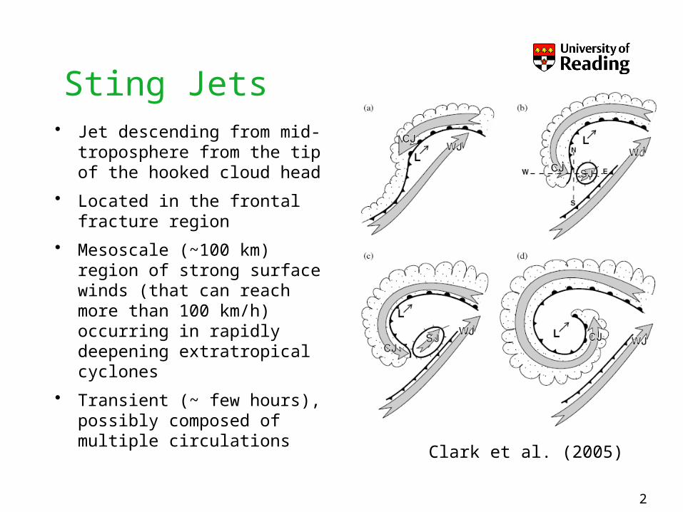
Storm Anna:Sting jet history along trajectories

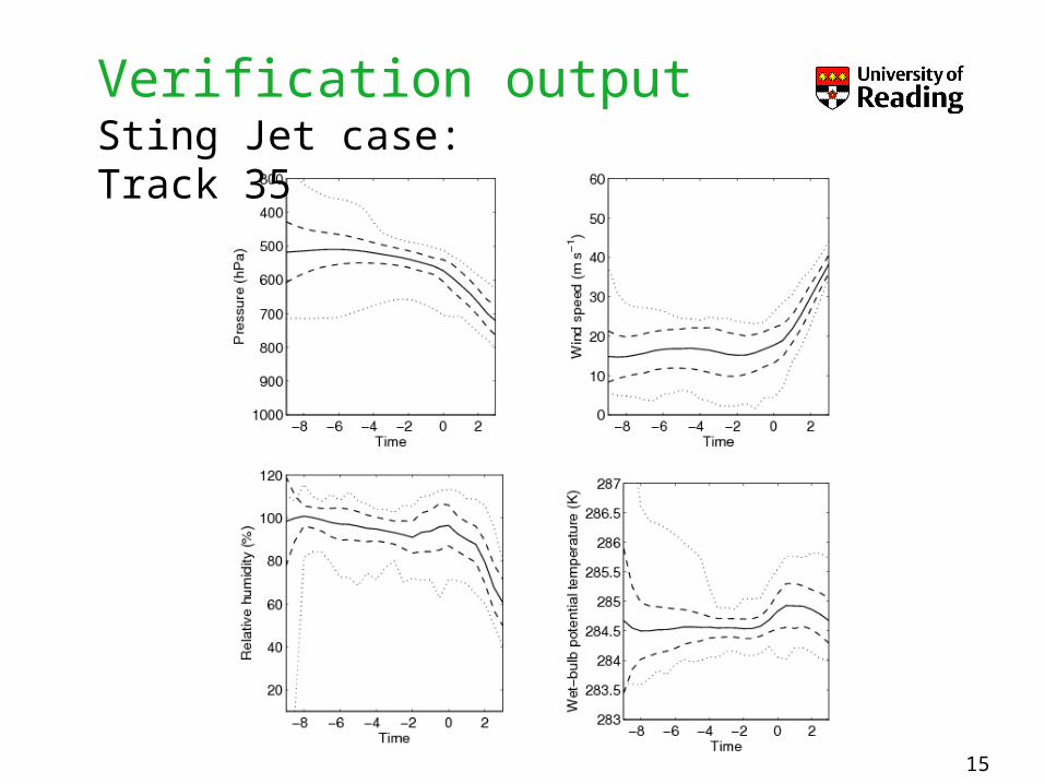
Time series along Lagrangian trajectories following the sting jet showing the ensemble–mean (solid), ensemble-mean plus/minus one standard deviation (dashed) and instantaneous maxima and minima (dotted) of (A) pressure and (B) relative humidity.

A B

4

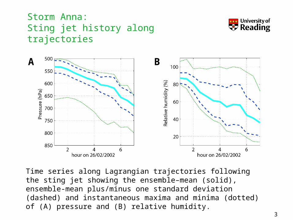
Storm Anna:Sting jet history along trajectories

Time series along trajectories following the sting jet showing the ensemble–mean (solid), ensemble-mean plus/minus one standard deviation (dashed) and instantaneous maxima and minima (dotted) of (A) wet-bulb potential temperature, (B) potential temperature, and (C) specific humidity.

A B

C

5

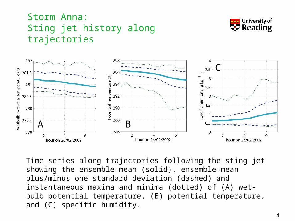
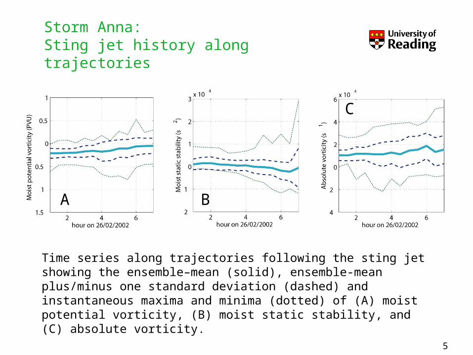
Storm Anna:Sting jet history along trajectories

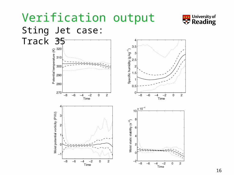
Time series along trajectories following the sting jet showing the ensemble–mean (solid), ensemble-mean plus/minus one standard deviation (dashed) and instantaneous maxima and minima (dotted) of (A) moist potential vorticity, (B) moist static stability, and (C) absolute vorticity.

A B

C

6

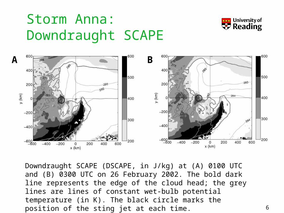
Storm Anna:Downdraught SCAPE

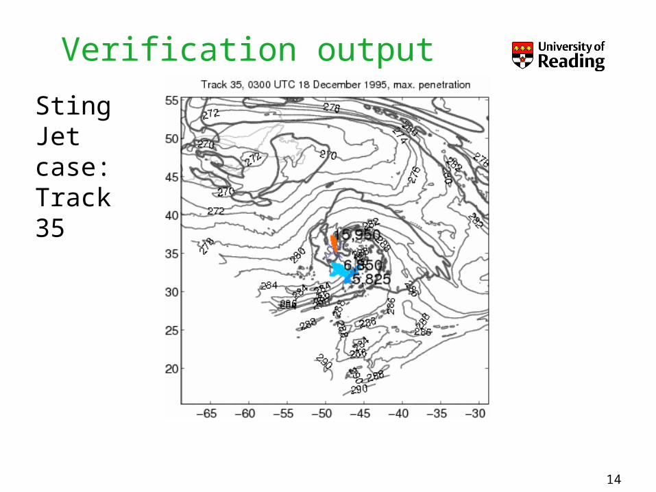
Downdraught SCAPE (DSCAPE, in J/kg) at (A) 0100 UTC and (B) 0300 UTC on 26 February 2002. The bold dark line represents the edge of the cloud head; the grey lines are lines of constant wet-bulb potential temperature (in K). The black circle marks the position of the sting jet at each time.

A B

• Minimum DSCAPE descending from the mid-troposphere

– DSCAPE > Emin J kg-1

• Search restricted to upper levels

– pstart < Pmax hPa

• Moisture needed to precipitate over unstable areas with large DSCAPE

– RH > RHmax %

• Location within a fractured cold front

A climatology of sting jets

1min K kmw G 1

min K swv A

7

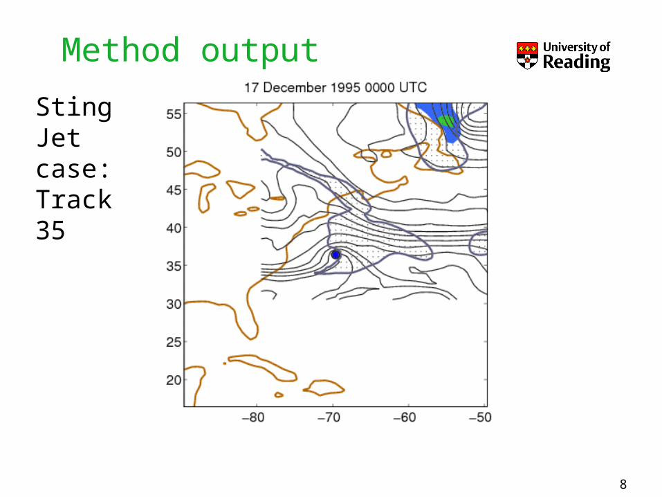
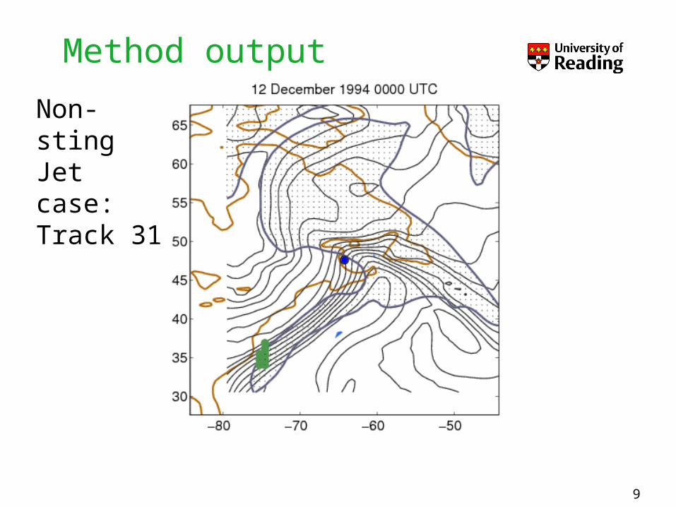
Method output

8

Sting Jet case:Track 35

Method output

9

Non-sting Jet case:Track 31

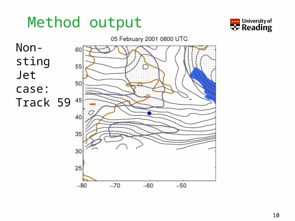
Method output

10

Non-sting Jet case:Track 59

• 100 most intense cyclones (classified by absolute vorticity) in winter months (DJF) in ERA-Interim (1989—2009).

• 23 cyclones present instability in the proximity of the cyclone centre.

• This instability is not always located in optimal locations to generate to sting jets

Results from ERA-Interim

11

• No available surface wind dataset with appropriate temporal and spatial resolution

• Verification method relies on high-resolution LAM simulations (12 km)

• The techniques are the same used in previous case studies

– Identification of regions of dry, strong winds close to the surface, and in the frontal fracture region

– Backward trajectories starting from (ending up at) those regions

• Very computationally expensive

Verification

12

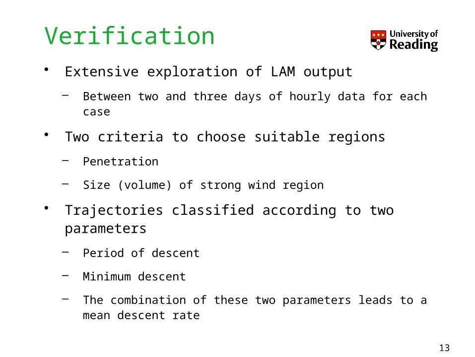
• Extensive exploration of LAM output

– Between two and three days of hourly data for each case

• Two criteria to choose suitable regions

– Penetration

– Size (volume) of strong wind region

• Trajectories classified according to two parameters

– Period of descent

– Minimum descent

– The combination of these two parameters leads to a mean descent rate

Verification

13

Verification output

14

Sting Jet case:Track 35

Verification output

15

Sting Jet case: Track 35

Verification output

16

Sting Jet case: Track 35

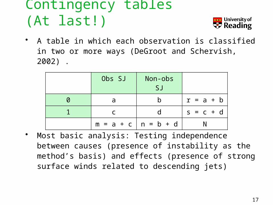
• A table in which each observation is classified in two or more ways (DeGroot and Schervish, 2002) .

• Most basic analysis: Testing independence between causes (presence of instability as the method’s basis) and effects (presence of strong surface winds related to descending jets)

Contingency tables (At last!)

17

Obs SJ Non-obs SJ

0 a b r = a + b

1 c d s = c + d

m = a + c n = b + d N

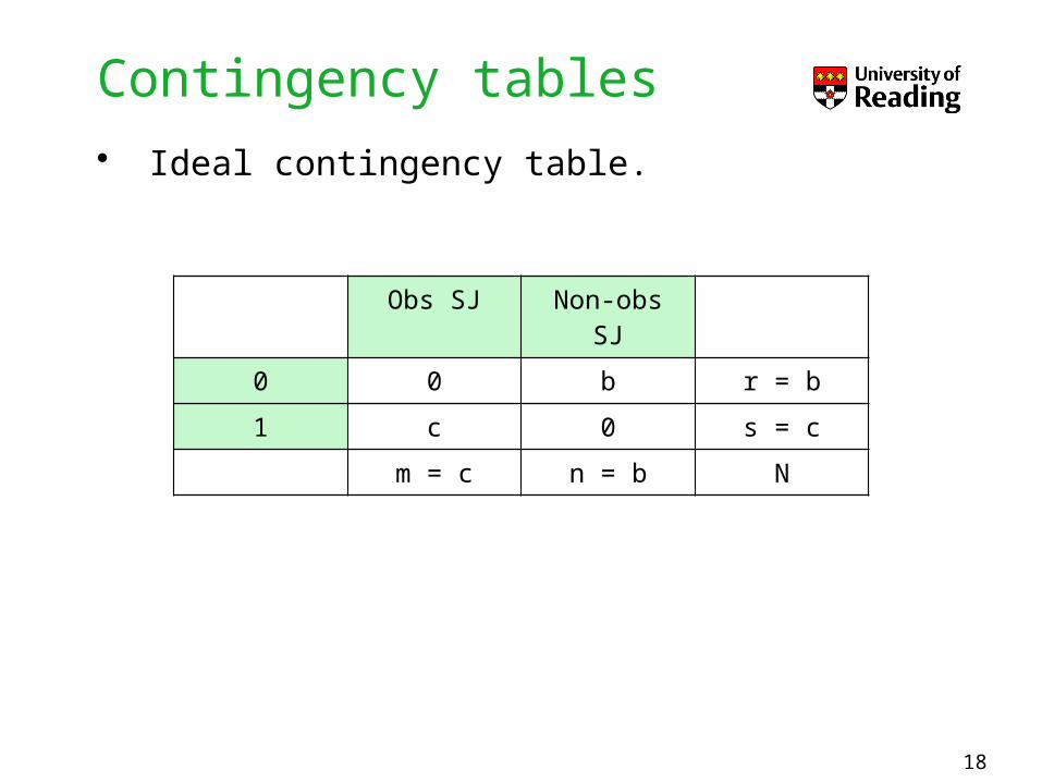
• Ideal contingency table.

Contingency tables

18

Obs SJ Non-obs SJ

0 0 b r = b

1 c 0 s = c

m = c n = b N

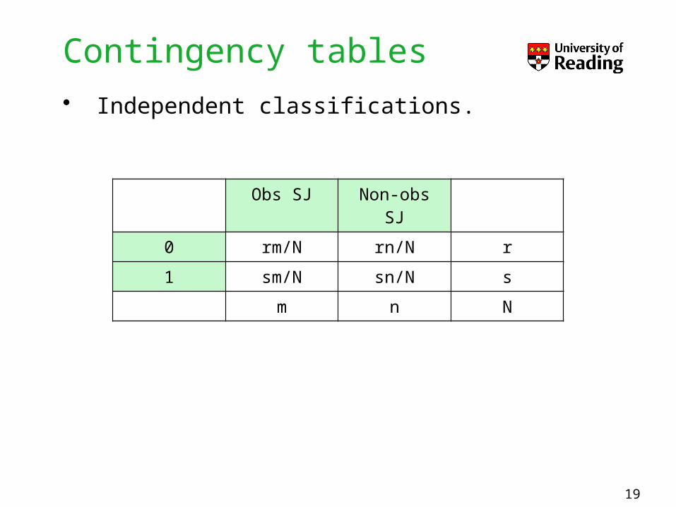
• Independent classifications.

Contingency tables

19

Obs SJ Non-obs SJ

0 rm/N rn/N r

1 sm/N sn/N s

m n N

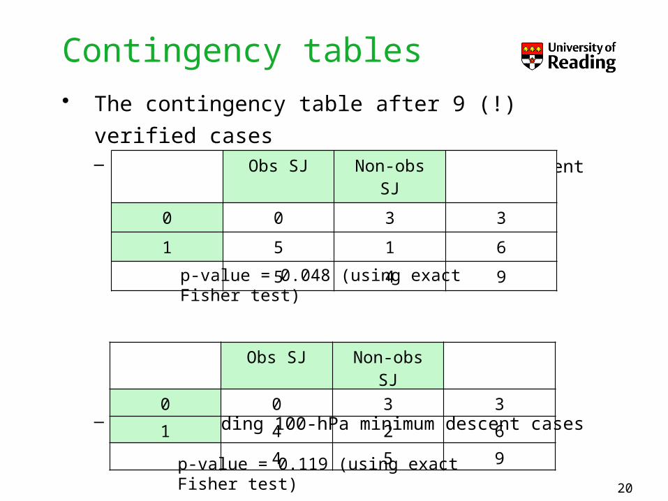
• The contingency table after 9 (!) verified cases– Including 100-hPa and 50-hPa minimum descent cases

– Only including 100-hPa minimum descent cases

Contingency tables

20

Obs SJ Non-obs SJ

0 0 3 3

1 5 1 6

5 4 9

p-value = 0.048 (using exact Fisher test)

Obs SJ Non-obs SJ

0 0 3 3

1 4 2 6

4 5 9

p-value = 0.119 (using exact Fisher test)

Final remarks• Even with very few results the method to find

instability associated with sting jets is giving satisfactory results.

• Many more verified cases are also necessary to properly characterise a contingency table.

• The amount of data can be useful for more extensive sting-jet (and extra-tropical cyclone) studies.

References

1. Clark, P. A., K. A. Browning, and C. Wang, 2005: The sting at the end of the tail: Model diagnostics of fine-scale three-dimensional structure of the cloud head. Quart. J. Roy. Meteor. Soc., 131, 2263-2292.

2. DeGroot, M.H. and M. J. Schervish, 2002: Probability and statistics. (3rd ed.). Addison-Wesley.