TUM-HEP-467/02

A Flavor Symmetry Model for Bilarge

Leptonic Mixing and the Lepton Masses

Tommy Ohlsson a,1, Gerhart Seidl a,2

aInstitut fur Theoretische Physik, Physik-Department, Technische UniversitatMunchen, James-Franck-Straße, 85748 Garching bei Munchen, Germany

Abstract

We present a model for leptonic mixing and the lepton masses based on flavorsymmetries and higher-dimensional mass operators. The model predicts bilarge lep-tonic mixing (i.e., the mixing angles θ12 and θ23 are large and the mixing angleθ13 is small) and an inverted hierarchical neutrino mass spectrum. Furthermore, itapproximately yields the experimental hierarchical mass spectrum of the chargedleptons. The obtained values for the leptonic mixing parameters and the neutrinomass squared differences are all in agreement with atmospheric neutrino data, theMikheyev–Smirnov–Wolfenstein large mixing angle solution of the solar neutrinoproblem, and consistent with the upper bound on the reactor mixing angle. Thus,we have a large, but not close to maximal, solar mixing angle θ12, a nearly maximalatmospheric mixing angle θ23, and a small reactor mixing angle θ13. In addition,the model predicts θ12 ' π

4 − θ13.

Key words: neutrino mass models, leptonic mixing, neutrino masses, chargedlepton masses, flavor symmetries, higher-dimensional operatorsPACS: 14.60.Pq, 11.30.Hv, 12.15.Ff

1 E-mail: tohlsson@ph.tum.de2 E-mail: gseidl@ph.tum.de

11 June 2002

1 Introduction

The fermionic sector of the standard model (SM) of elementary particle physicsis described by 13 renormalized parameters (6 quark masses, 3 charged lep-ton masses, 3 CKM mixing angles 3 , and one CP violation phase). Obviously,these parameters are not arbitrary, but exhibit relations which can only be un-derstood when going beyond the SM. One possibility to obtain realistic quarkmasses and CKM mixing angles in an extension of the SM is to introduceflavor symmetries that are sequentially broken. At the first glance, the hier-archical mass spectra of the quarks and the charged leptons actually suggestunderlying non-Abelian flavor symmetry groups acting on the first and secondgenerations only. 4 However, in the light of recent atmospheric [5–9] and so-lar [10–17] neutrino experimental results, it seems to be difficult to extend thisidea to the neutrinos. Especially, the result that, among the different possiblesolutions of the solar neutrino problem, the Mikheyev–Smirnov–Wolfenstein(MSW) [18–20] large mixing angle (LMA) solution is the presently preferredone [21–23], draws a picture of the involved flavor symmetries and their break-ing mechanisms that differs remarkably from the early approaches, which havebeen applied to the quark sector. In the “standard” parameterization, theMSW LMA solution implies that we have a bilarge mixing scenario in thelepton sector in which the solar mixing angle θ12 is large, but not necessarilyclose to maximal, the atmospheric mixing angle θ23 is nearly maximal, andthe reactor mixing angle θ13 is small. Clearly, this is in sharp contrast to thequark sector in which all mixing angles are small [24] and it indicates that theflavor symmetries act on the third generation too.

By assuming only an Abelian U(1) flavor symmetry, one obtains that the at-mospheric mixing angle may be large, but cannot be enforced to be nearlymaximal [25–27]. Therefore, a natural close to maximal νµ-ντ -mixing can beinterpreted as a strong hint for some underlying non-Abelian flavor symme-try acting on the second and third generations [28,29]. Neutrino mass modelswhich give large or maximal solar and atmospheric mixing angles by puttingthe second and third generations of the leptons into the regular representa-tion of the symmetric group S2 [30] or into the irreducible two-dimensionalrepresentation of the symmetric group S3 [31] are, in general, plagued witha fine-tuning problem in the charged lepton sector, since they tend to pre-dict the muon and tau masses to be of the same order of magnitude, i.e.,they lack providing an understanding of the hierarchical mass spectrum in the

3 The mixing angles in the quark sector are usually called the Cabibbo–Kobayashi–Maskawa (CKM) mixing angles [1, 2].4 By placing the first two generations into irreducible representations of flavor sym-metries, one can in supersymmetric models achieve near degeneracy of the corre-sponding squark masses thus suppressing large flavor changing neutral currents [3,4].

2

charged lepton sector. A recently proposed model based on an SU(3) flavorsymmetry [4] gives approximately bimaximal leptonic mixing as well as a suc-cessful description of the charged fermion masses, but predicts the presentlydisfavored MSW low mass (LOW) or vacuum oscillation (VAC) solution ofthe solar neutrino problem. Similarly, the highly predictive models of flavordemocracy [32–39] yield large solar and atmospheric mixing angles, but fitthe LOW or VAC solution rather than the MSW LMA solution [40]. In grandunified theory model building, it seems that the MSW LMA solution witha normal hierarchical neutrino mass spectrum is more natural than with aninverted one [41] (for a recent phenomenological analysis of minimal schemesfor the MSW LMA solution with inverted hierarchical neutrino mass spectra,see, e.g., Ref. [42]). Also from empirical lepton and quark mass spectra anal-yses a normal hierarchical (or inverse hierarchical) neutrino mass spectrumseems to be rather plausible [43]. A comparably simple way of generating theMSW LMA solution with normal hierarchical neutrino mass spectra is, e.g.,provided by models based on single right-handed neutrino dominance [44].

In a previous Letter [45], we introduced a model for bilarge leptonic mixingbased on higher-dimensional operators, using the Froggatt–Nielsen mecha-nism, and Abelian horizontal flavor symmetries of continuous and discretetypes. In this paper, we consider a modified and extended version of thismodel and we explicitly demonstrate the vacuum alignment mechanism, whichproduces a nearly maximal atmospheric mixing angle θ23 as well as a large,but not close to maximal, solar mixing angle θ12, as required by the MSWLMA solution. Simultaneously, the vacuum alignment mechanism generatesa strictly hierarchical charged lepton mass spectrum thus resolving the fine-tuning problem many realistic models, which seek to predict the MSW LMAsolution, are suffering from. Furthermore, this model gives a small mixing ofthe first and second generations of the charged leptons, which is comparablewith the mixing of the quarks, whereas the mixing among the neutrinos isessentially bimaximal [46]. The actual leptonic mixing angles are then a resultof combining the contributions coming from both the charged leptons and theneutrinos (see Fig. 1). Thus, the model predicts the relation θ12 ' π

4− θ13

between the solar mixing angle θ12 and the reactor mixing angle θ13, which isnon-zero and lies in the range of the quark mixing angles.

Note that our study assumes that there are three neutrino flavors, and there-fore, three neutrino flavor states να (α = e, µ, τ) and also three neutrino masseigenstates νa (a = 1, 2, 3). Furthermore, it assumes that all CP violationphases are equal to zero.

The paper is organized as follows: In Sec. 2, we introduce the representationcontent of our model including U(1) charges and discrete symmetries. Themulti-scalar potential of the model is then analyzed in Sec. 3, where we ex-plicitly demonstrate the vacuum alignment mechanism. Next, in Secs. 4 and 5,

3

U l U ν

Neutrino masssquared differences

Leptonic mixingparameters

Charged leptonmasses

Transformation into"standard" parameterization

Neutrino mixingparameters

Charged leptonmixing parameters

lM

l ν

M ν

U

Diagonalization

U = U Ul ν✝

M M

Theory or model

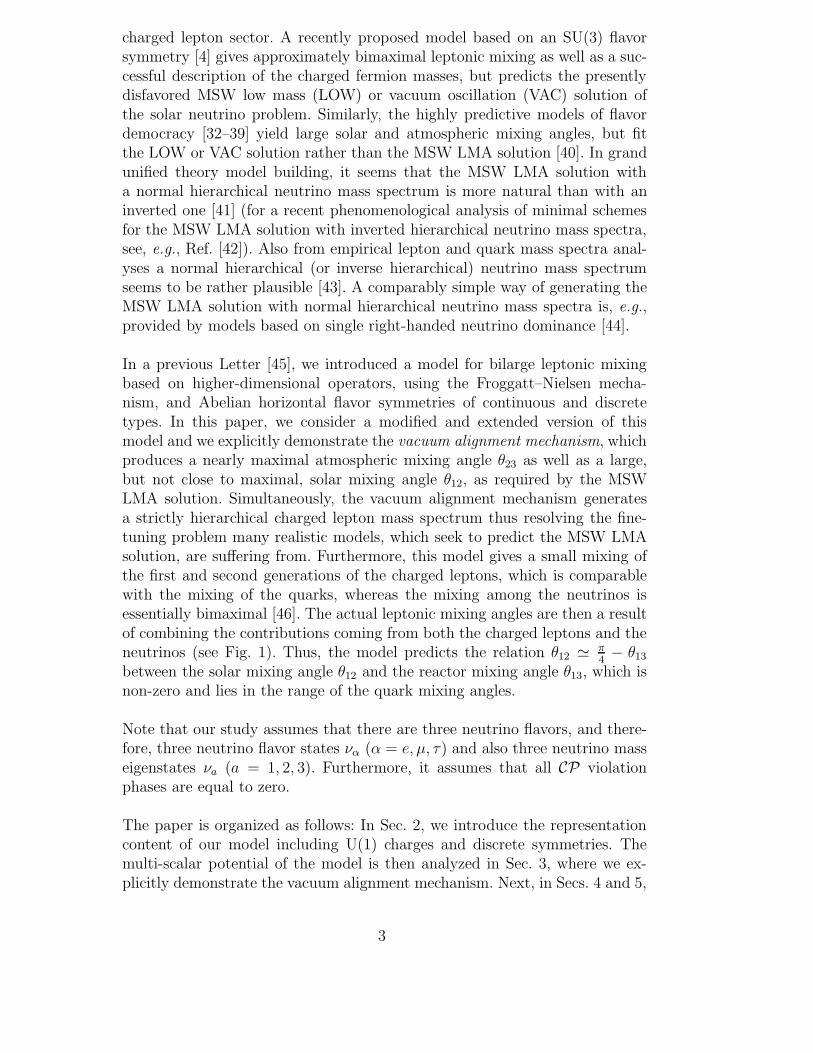
Fig. 1. Flow-scheme for computing leptonic mixing parameters and lepton massesfrom any given charged lepton and neutrino mass matrices.

the Yukawa interactions of the charged leptons and neutrinos, respectively, areinvestigated and discussed, which lead to the mass matrices of the correspond-ing particles. In Sec. 6, the lepton mass matrices are diagonalized yielding thecharged lepton masses and the neutrino mass squared differences as well asthe charged lepton and neutrino mixing angles (see again Fig. 1). In Sec. 7,the total leptonic mixing angles are derived and calculated. Implications forneutrinoless double β-decay, astrophysics, and cosmology are briefly studiedin Sec. 8. Finally, in Sec. 9, we present a summary as well as our conclusions.In addition, we present in the Appendix a scheme for how to transform anygiven 3 × 3 unitary matrix to the “standard” parameterization form of theParticle Data Group [24].

2 The representation content

Let us consider an extension of the SM in which the lepton masses are gener-ated by higher-dimensional operators [47,48] via the Froggatt–Nielsen mecha-nism [49]. (A classification of effective neutrino mass operators has been givenin Ref. [50].) Since we are mainly concerned with the question of whether thereis a possible naturally maximal νµ-ντ -mixing in the MSW LMA solution ornot, for which the properties of the quarks are seemingly irrelevant, we will,

4

for simplicity and without loss of generality, omit the quark sector in our fur-ther discussion. For a recent related study including also the quark sector, see,e.g., Refs. [51, 52]. In a self-explanatory notation, we will denote the lepton

doublets as Lα = (ναL eαL), where α = e, µ, τ , and the right-handed charged

leptons as Eα = eαR, where α = e, µ, τ . The part of the scalar sector, whichcarries non-zero SM quantum numbers, consists of two Higgs doublets H1 andH2, where H1 couples to the neutrinos and H2 to the charged leptons. Thiscan be achieved by assuming, e.g., a discrete Z2 symmetry under which H2

and Eα (α = e, µ, τ) are odd and H1 and the rest of the SM fields are even.The masses of the charged leptons arise through the mixing with additionalheavy right-handed charged fermions, which all have masses of the order ofmagnitude of some characteristic mass scale M1. Apart from some generalprescriptions of their transformations under the flavor symmetries, which willbe introduced below, it is not necessary to explicitly present the fundamentaltheory of these additional (or extra) charged fermions. This is in contrast tothe neutrino sector, which we will extend by five additional heavy SM sin-glet Dirac neutrinos Ne, Nµ, Nτ , F1, and F2. The neutrinos F1 and F2 aresupposed to have masses of the same order M1 as the charged intermediateFroggatt–Nielsen states, whereas Ne, Nµ, and Nτ all have masses of the orderof magnitude of some relevant high (unification) mass scale M2. While M2

takes the role of some seesaw scale [53–55] (and it is therefore responsible forthe smallness of the neutrino masses), M1 can be as low as several TeV [56,57].In order to obtain the structures of the lepton mass matrices from an under-lying symmetry principle in the context of a renormalizable field theory, wewill furthermore extend the scalar sector by additional SM singlet scalar fieldsφ1, φ2, . . . , φ10, φ′1, φ

′2, . . . , φ′6, and θ and we will assign these fields gauged

horizontal U(1) charges Q1, Q2, and Q3 as follows:

(Q1, Q2, Q3)

Le,Ee (1, 0, 0)

Lµ,Lτ ,Eµ,Eτ (0, 1, 0)

Ne (1, 0, 0)

Nµ, Nτ (0, 1, 0)

F1 (1, 0, 0)

F2 (−1, 0, 1)

H1, H2 (0, 0, 0)

φ1, φ2 (1,−1, 2)

φ3, φ4 (0, 0, 0)

φ5, φ6 (0, 0, 1)

φ′1, φ′2, φ′3, φ′4, φ′5, φ′6 (0, 0, 0)

φ7, φ8 (−1,−1, 0)

φ9 (−2, 0, 1)

φ10 (0, 0, 0)

θ (0, 0,−1)

5

In the rest of the paper, it will always be understood that the Higgs dou-blets H1 and H2 are total singlet under transformations of other additionalsymmetries. Note that our model is kept free from chiral anomalies, since thefermions transform as vector-like pairs under the extra U(1) charges.

The first generation of the charged leptons is distinguished from the secondand third generations if we require for P ≡ e2πi/n, where the integer n obeysn ≥ 5, invariance of the Lagrangian under transformation of the following Zn

symmetry:

D1 :

Ee → P−4Ee, Eµ → P−1Eµ, Eτ → P−1Eτ ,

φ1 → Pφ1, φ2 → Pφ2,

φ3 → Pφ3, φ4 → Pφ4,

φ5 → Pφ5, φ6 → Pφ6,

(1)

where we assume that the fields Ne, Nµ, Nτ , F1, and F2 are singlets undertransformation of the symmetry D1. In addition, the symmetry D1 forbidsthe fields φ1, φ2, . . . , φ6 to participate in the leading order mass terms for theneutrinos. Furthermore, the permutation symmetries

D2 :

Lµ → −Lµ, Eµ → −Eµ,

Nµ → −Nµ,

φ′1 ↔ φ′2, φ1 ↔ φ2,

φ7 → −φ7,

(2)

D3 :

Lµ → −Lµ, Nµ → −Nµ,

φ′3 ↔ φ′4, φ3 ↔ φ4,

φ′5 ↔ φ′6, φ5 ↔ φ6,

φ7 → −φ7,

(3)

D4 :

Lµ ↔ Lτ , Eµ ↔ Eτ ,

Nµ ↔ Nτ ,

φ2 → −φ2, φ4 → −φ4, φ6 → −φ6,

φ7 ↔ φ8

(4)

are responsible for generating a naturally maximal atmospheric mixing angle,since they establish exact degeneracies of the Yukawa couplings in the leptonic

6

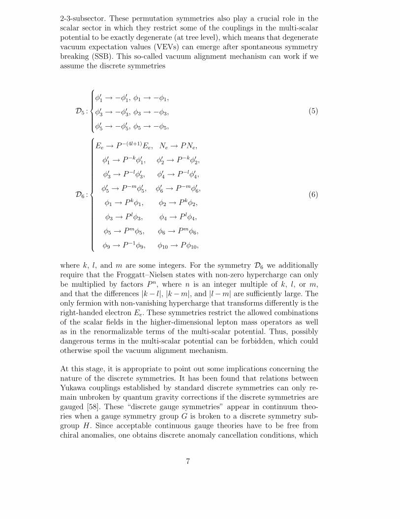
2-3-subsector. These permutation symmetries also play a crucial role in thescalar sector in which they restrict some of the couplings in the multi-scalarpotential to be exactly degenerate (at tree level), which means that degeneratevacuum expectation values (VEVs) can emerge after spontaneous symmetrybreaking (SSB). This so-called vacuum alignment mechanism can work if weassume the discrete symmetries

D5 :

φ′1 → −φ′1, φ1 → −φ1,

φ′3 → −φ′3, φ3 → −φ3,

φ′5 → −φ′5, φ5 → −φ5,

(5)

D6 :

Ee → P−(4l+1)Ee, Ne → PNe,

φ′1 → P−kφ′1, φ′2 → P−kφ′2,

φ′3 → P−lφ′3, φ′4 → P−lφ′4,

φ′5 → P−mφ′5, φ′6 → P−mφ′6,

φ1 → P kφ1, φ2 → P kφ2,

φ3 → P lφ3, φ4 → P lφ4,

φ5 → P mφ5, φ6 → P mφ6,

φ9 → P−1φ9, φ10 → Pφ10,

(6)

where k, l, and m are some integers. For the symmetry D6 we additionallyrequire that the Froggatt–Nielsen states with non-zero hypercharge can onlybe multiplied by factors P n, where n is an integer multiple of k, l, or m,and that the differences |k− l|, |k−m|, and |l−m| are sufficiently large. Theonly fermion with non-vanishing hypercharge that transforms differently is theright-handed electron Ee. These symmetries restrict the allowed combinationsof the scalar fields in the higher-dimensional lepton mass operators as wellas in the renormalizable terms of the multi-scalar potential. Thus, possiblydangerous terms in the multi-scalar potential can be forbidden, which couldotherwise spoil the vacuum alignment mechanism.

At this stage, it is appropriate to point out some implications concerning thenature of the discrete symmetries. It has been found that relations betweenYukawa couplings established by standard discrete symmetries can only re-main unbroken by quantum gravity corrections if the discrete symmetries aregauged [58]. These “discrete gauge symmetries” appear in continuum theo-ries when a gauge symmetry group G is broken to a discrete symmetry sub-group H . Since acceptable continuous gauge theories have to be free fromchiral anomalies, one obtains discrete anomaly cancellation conditions, which

7

strongly constrain the massless fermion content of the theory [59]. At a morefundamental level, this implies for our model that the permutation symme-tries must actually be gauged, since the relations, which are based on them,will prove to be crucial for obtaining essentially strict maximal atmosphericmixing. However, it is interesting to note that in M-theory, one expects thediscrete symmetries to be always anomaly-free [60].

3 The multi-scalar potential

3.1 The two-Higgs doublet potential

From the most general two-Higgs doublet potential of the fields H1 and H2

(for an extensive review on electroweak Higgs potentials, see, e.g., Ref. [61]) weconclude that, in presence of the Z2 symmetry, which distinguishes between H1

and H2 (see Sec. 2), each of these fields appears only to the second or fourthpower in the multi-scalar potential. Hence, in any renormalizable terms ofthe multi-scalar potential, which mix H1 or H2 with the SM singlet scalarfields, the Higgs doublets are only allowed to appear in terms of their absolutesquares |H1|2 and |H2|2. Next, since the Higgs doublets carry zero Q1, Q2,and Q3 charges and are Di-singlets, where i = 1, 2, . . . , 6, there exists a rangeof parameters in the multi-scalar potential for which the standard two-Higgselectroweak symmetry breaking is possible. Furthermore, this implies that wecan, without loss of generality, separate the SM singlet scalar part from theHiggs-doublet part in the multi-scalar potential by formally absorbing theabsolute squares of the VEVs |〈H1〉|2 and |〈H2〉|2 into the coupling constantsof the mixed terms. Then, since the vacuum alignment mechanism of the SMsinglet fields is independent from the details of the Higgs doublet physics,we can in what follows discard the effects of the Higgs doublets and fullyconcentrate on the properties of the SM singlet scalar fields.

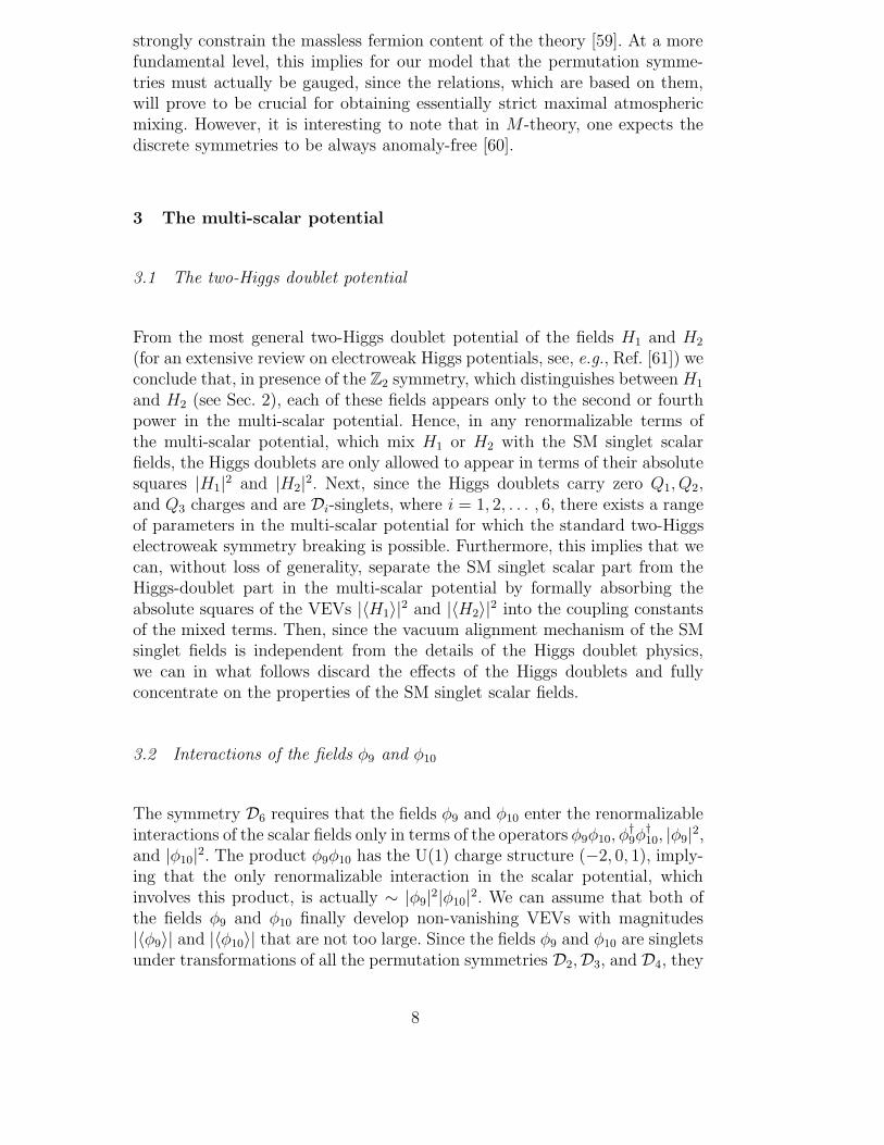
3.2 Interactions of the fields φ9 and φ10

The symmetry D6 requires that the fields φ9 and φ10 enter the renormalizableinteractions of the scalar fields only in terms of the operators φ9φ10, φ

†9φ

†10, |φ9|2,

and |φ10|2. The product φ9φ10 has the U(1) charge structure (−2, 0, 1), imply-ing that the only renormalizable interaction in the scalar potential, whichinvolves this product, is actually ∼ |φ9|2|φ10|2. We can assume that both ofthe fields φ9 and φ10 finally develop non-vanishing VEVs with magnitudes|〈φ9〉| and |〈φ10〉| that are not too large. Since the fields φ9 and φ10 are singletsunder transformations of all the permutation symmetries D2,D3, and D4, they

8

will have no effect on the relative alignment of the rest of the scalar fields, be-cause they enter the corresponding interactions only in terms of the absolutesquares |〈φ9〉|2 and |〈φ10〉|2. For this reason we will, without loss of generality,discard the terms in the scalar potential which involve the fields φ9 and φ10 inour considerations.

From the assignment of the U(1) charges Q1, Q2, and Q3 and the symme-try D6 (which does not permute any of the fields) it follows that any renor-malizable term in the scalar potential which involves the SM singlet fieldsφ1, φ2, φ5, φ6, φ7, φ8, or θ can only be allowed if these fields appear in one ofthe following combinations:

φ1,2φ†1,2 , φ5,6φ

†5,6 , φ5,6θ , φ7,8φ

†7,8 , |θ|2 , (7)

where “φi,j” (i, j = 1, 2, . . . , 8) denotes some linear combination of the fields φi

and φj. Among the products in Eq. (7) only the product φ5,6θ transforms non-trivially under the symmetry D1. In addition, since the fields φ′1, φ

′2, . . . , φ′6

are D1-singlets, we observe that the fields φ3 and φ4, which carry a non-zero D1-charge, can only appear either in the combination φ3,4φ

†3,4 or in the

combination φ†3,4φ5,6θ. However, the latter combination is forbidden by D6-invariance.

3.3 Interactions of the field θ

As in Sec. 3.2, we can assume that the field θ finally develops a non-vanishingVEV with a magnitude |〈θ〉| that is not too large. Except for the combinationφ5,6θ in Eq. (7) all scalar interactions involve an equal number (0, 1, or 2) ofthe fields θ and its adjoint θ†, which can then be paired to the absolute square|θ|2. Since the interaction φ5,6θ|θ|2 is forbidden by the symmetries D1 andD6 and θ is a total singlet under transformations of the discrete symmetriesD1,D2, . . . ,D6, all terms which involve the absolute square |θ|2 will have noinfluence on the relative alignment of the rest of the scalar fields. For thisreason we can, without loss of generality, omit the terms in the scalar potentialwhich involve |θ|2 in our considerations.

3.4 Interactions of the fields φ7 and φ8

From the U(1) charge assignment we conclude that only an even number ofthe fields φ7 and φ8 (or their complex conjugates) can participate in the scalarinteractions. Let us now especially consider the operator φ†7φ8 (or equivalentlyits complex conjugate). Under application of each of the symmetries D2 andD3 the operator φ†7φ8 changes sign. Therefore, the symmetry D2 requires this

9

operator to couple to one of the fields taken from the set {φ′1, φ′2, φ1, φ2, φ7}. Si-multaneously, the symmetry D3 requires this operator to couple only to fieldstaken from the extended set {φ′3, φ′4, φ′5, φ′6, φ3, φ4, φ5, φ6, φ7}. Both conditionscan only be fulfilled if the operator φ†7φ8 couples to the field φ7 or its com-plex conjugate, but not to the operator products (φ7)

2, (φ†7)2, or |φ7|2. Since

the product φ†7φ8 carries the U(1) charges (0, 0, 0), the operator φ†7φ8 can onlycouple to some linear combination of the operators φ7φ

†8 and φ8φ

†7. As a conse-

quence, if a general operator φ7,8φ†7,8 enters an interaction with scalars, which

are different from the fields φ7 and φ8, then this operator φ7,8φ†7,8 is a linear

combination of the absolute squares |φ7|2 and |φ8|2.

Let us denote by φi and φj two scalar fields, which are different from the fields

φ7 and φ8. Taking Eq. (7) and the operator φ3,4φ†3,4 into account, the operator

product φiφj must be of one of the following types:

φ1,2φ†1,2 , φ3,4φ

†3,4 , φ5,6φ

†5,6 , φ′1,2φ

′†1,2 , φ′3,4φ

′†3,4 , φ′5,6φ

′†5,6 , (8)

where the last three combinations follow from the D6-invariance. Next, thesymmetry D5 implies that φj = φ†i for the combinations in Eq. (8), i.e., theproduct is the absolute square φiφj = |φi|2. Using the result of the previousparagraph, invariance under transformation of the symmetry D4 gives for themost general interactions of the fields φ7 and φ8 with the other scalar fieldsthe terms

(|φ7|2 + |φ8|2)∑

ϕi 6=φ7,φ8

ci|ϕi|2, (9)

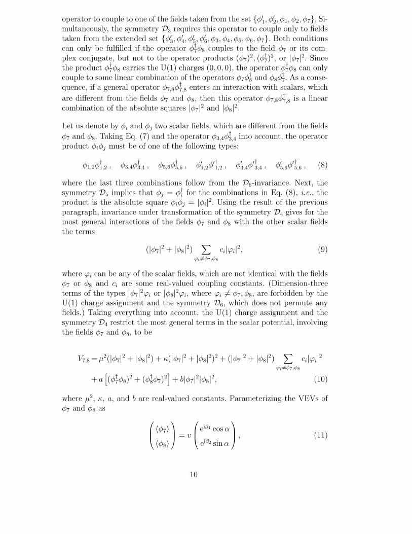
where ϕi can be any of the scalar fields, which are not identical with the fieldsφ7 or φ8 and ci are some real-valued coupling constants. (Dimension-threeterms of the types |φ7|2ϕi or |φ8|2ϕi, where ϕi 6= φ7, φ8, are forbidden by theU(1) charge assignment and the symmetry D6, which does not permute anyfields.) Taking everything into account, the U(1) charge assignment and thesymmetry D4 restrict the most general terms in the scalar potential, involvingthe fields φ7 and φ8, to be

V7,8 =µ2(|φ7|2 + |φ8|2) + κ(|φ7|2 + |φ8|2)2 + (|φ7|2 + |φ8|2)∑

ϕi 6=φ7,φ8

ci|ϕi|2

+ a[(φ†7φ8)

2 + (φ†8φ7)2]+ b|φ7|2|φ8|2, (10)

where µ2, κ, a, and b are real-valued constants. Parameterizing the VEVs ofφ7 and φ8 as

〈φ7〉〈φ8〉

= v

eiβ1 cos α

eiβ2 sin α

, (11)

10

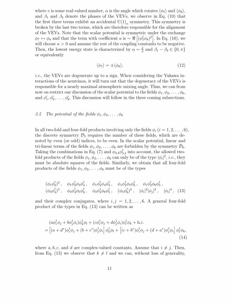
where v is some real-valued number, α is the angle which rotates 〈φ7〉 and 〈φ8〉,and β1 and β2 denote the phases of the VEVs, we observe in Eq. (10) thatthe first three terms exhibit an accidental U(1)α symmetry. This symmetry isbroken by the last two terms, which are therefore responsible for the alignmentof the VEVs. Note that the scalar potential is symmetric under the exchangeφ7 ↔ φ8 and that the term with coefficient a is ∼ <

[(φ†7φ8)

2]. In Eq. (10), we

will choose κ > 0 and assume the rest of the coupling constants to be negative.Then, the lowest energy state is characterized by α = π

4and β1 − β2 ∈ {0, π}

or equivalently

〈φ7〉 = ±〈φ8〉, (12)

i.e., the VEVs are degenerate up to a sign. When considering the Yukawa in-teractions of the neutrinos, it will turn out that the degeneracy of the VEVs isresponsible for a nearly maximal atmospheric mixing angle. Thus, we can fromnow on restrict our discussion of the scalar potential to the fields φ1, φ2, . . . , φ6,and φ′1, φ

′2, . . . , φ′6. This discussion will follow in the three coming subsections.

3.5 The potential of the fields φ1, φ2, . . . , φ6

In all two-fold and four-fold products involving only the fields φi (i = 1, 2, . . . , 6),the discrete symmetry D5 requires the number of these fields, which are de-noted by even (or odd) indices, to be even. In the scalar potential, linear andtri-linear terms of the fields φ1, φ2, . . . , φ6 are forbidden by the symmetry D6.Taking the combinations in Eq. (7) and φ3,4φ

†3,4 into account, the allowed two-

fold products of the fields φ1, φ2, . . . , φ6 can only be of the type |φi|2, i.e., theymust be absolute squares of the fields. Similarly, we obtain that all four-foldproducts of the fields φ1, φ2, . . . , φ6 must be of the types

(φ1φ†2)

2 , φ1φ†2φ3φ

†4 , φ1φ

†2φ4φ

†3 , φ1φ

†2φ5φ

†6 , φ1φ

†2φ6φ

†5 ,

(φ3φ†4)

2 , φ3φ†4φ5φ

†6 , φ3φ

†4φ6φ

†5 , (φ5φ

†6)

2 , |φi|2|φj|2 , |φi|4 , (13)

and their complex conjugates, where i, j = 1, 2, . . . , 6. A general four-foldproduct of the types in Eq. (13) can be written as

(aφ†iφj + bφ†jφi)φ†kφl + (cφ†iφj + dφ†jφi)φ

†l φk + h.c.

=[(a + d∗)φ†iφj + (b + c∗)φ†jφi

]φ†kφl +

[(c + b∗)φ†iφj + (d + a∗)φ†jφi

]φ†l φk,

(14)

where a, b, c, and d are complex-valued constants. Assume that i 6= j. Then,from Eq. (13) we observe that k 6= l and we can, without loss of generality,

11

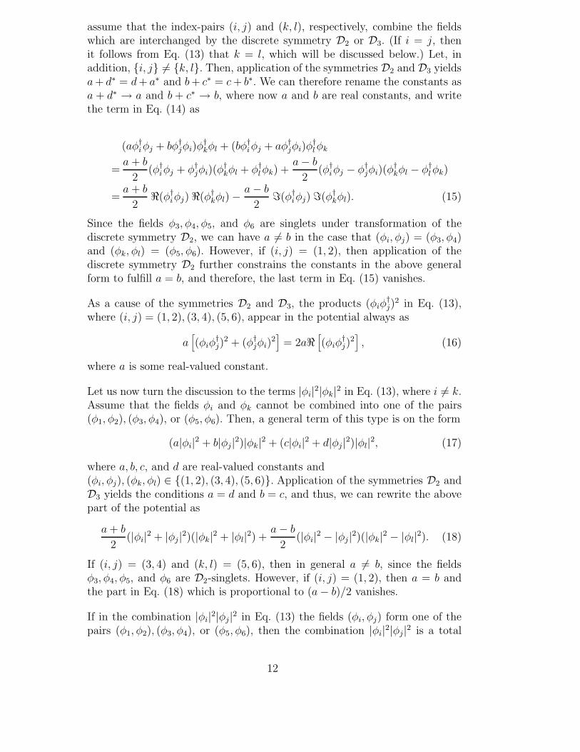
assume that the index-pairs (i, j) and (k, l), respectively, combine the fieldswhich are interchanged by the discrete symmetry D2 or D3. (If i = j, thenit follows from Eq. (13) that k = l, which will be discussed below.) Let, inaddition, {i, j} 6= {k, l}. Then, application of the symmetries D2 and D3 yieldsa + d∗ = d + a∗ and b + c∗ = c + b∗. We can therefore rename the constants asa + d∗ → a and b + c∗ → b, where now a and b are real constants, and writethe term in Eq. (14) as

(aφ†iφj + bφ†jφi)φ†kφl + (bφ†iφj + aφ†jφi)φ

†l φk

=a + b

2(φ†iφj + φ†jφi)(φ

†kφl + φ†l φk) +

a− b

2(φ†iφj − φ†jφi)(φ

†kφl − φ†l φk)

=a + b

2<(φ†iφj) <(φ†kφl)− a− b

2=(φ†iφj) =(φ†kφl). (15)

Since the fields φ3, φ4, φ5, and φ6 are singlets under transformation of thediscrete symmetry D2, we can have a 6= b in the case that (φi, φj) = (φ3, φ4)and (φk, φl) = (φ5, φ6). However, if (i, j) = (1, 2), then application of thediscrete symmetry D2 further constrains the constants in the above generalform to fulfill a = b, and therefore, the last term in Eq. (15) vanishes.

As a cause of the symmetries D2 and D3, the products (φiφ†j)

2 in Eq. (13),where (i, j) = (1, 2), (3, 4), (5, 6), appear in the potential always as

a[(φiφ

†j)

2 + (φ†jφi)2]

= 2a<[(φiφ

†j)

2], (16)

where a is some real-valued constant.

Let us now turn the discussion to the terms |φi|2|φk|2 in Eq. (13), where i 6= k.Assume that the fields φi and φk cannot be combined into one of the pairs(φ1, φ2), (φ3, φ4), or (φ5, φ6). Then, a general term of this type is on the form

(a|φi|2 + b|φj|2)|φk|2 + (c|φi|2 + d|φj|2)|φl|2, (17)

where a, b, c, and d are real-valued constants and(φi, φj), (φk, φl) ∈ {(1, 2), (3, 4), (5, 6)}. Application of the symmetries D2 andD3 yields the conditions a = d and b = c, and thus, we can rewrite the abovepart of the potential as

a + b

2(|φi|2 + |φj|2)(|φk|2 + |φl|2) +

a− b

2(|φi|2 − |φj|2)(|φk|2 − |φl|2). (18)

If (i, j) = (3, 4) and (k, l) = (5, 6), then in general a 6= b, since the fieldsφ3, φ4, φ5, and φ6 are D2-singlets. However, if (i, j) = (1, 2), then a = b andthe part in Eq. (18) which is proportional to (a− b)/2 vanishes.

If in the combination |φi|2|φj|2 in Eq. (13) the fields (φi, φj) form one of thepairs (φ1, φ2), (φ3, φ4), or (φ5, φ6), then the combination |φi|2|φj|2 is a total

12

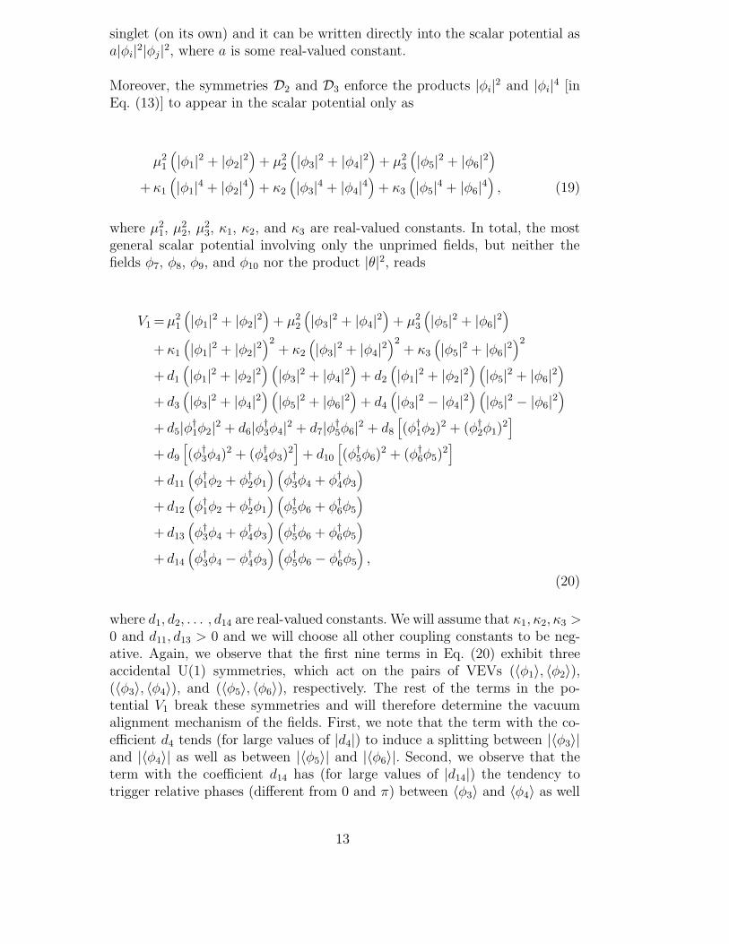
singlet (on its own) and it can be written directly into the scalar potential asa|φi|2|φj|2, where a is some real-valued constant.

Moreover, the symmetries D2 and D3 enforce the products |φi|2 and |φi|4 [inEq. (13)] to appear in the scalar potential only as

µ21

(|φ1|2 + |φ2|2

)+ µ2

2

(|φ3|2 + |φ4|2

)+ µ2

3

(|φ5|2 + |φ6|2

)+κ1

(|φ1|4 + |φ2|4

)+ κ2

(|φ3|4 + |φ4|4

)+ κ3

(|φ5|4 + |φ6|4

), (19)

where µ21, µ2

2, µ23, κ1, κ2, and κ3 are real-valued constants. In total, the most

general scalar potential involving only the unprimed fields, but neither thefields φ7, φ8, φ9, and φ10 nor the product |θ|2, reads

V1 = µ21

(|φ1|2 + |φ2|2

)+ µ2

2

(|φ3|2 + |φ4|2

)+ µ2

3

(|φ5|2 + |φ6|2

)+ κ1

(|φ1|2 + |φ2|2

)2+ κ2

(|φ3|2 + |φ4|2

)2+ κ3

(|φ5|2 + |φ6|2

)2

+ d1

(|φ1|2 + |φ2|2

) (|φ3|2 + |φ4|2

)+ d2

(|φ1|2 + |φ2|2

) (|φ5|2 + |φ6|2

)+ d3

(|φ3|2 + |φ4|2

) (|φ5|2 + |φ6|2

)+ d4

(|φ3|2 − |φ4|2

) (|φ5|2 − |φ6|2

)+ d5|φ†1φ2|2 + d6|φ†3φ4|2 + d7|φ†5φ6|2 + d8

[(φ†1φ2)

2 + (φ†2φ1)2]

+ d9

[(φ†3φ4)

2 + (φ†4φ3)2]+ d10

[(φ†5φ6)

2 + (φ†6φ5)2]

+ d11

(φ†1φ2 + φ†2φ1

) (φ†3φ4 + φ†4φ3

)+ d12

(φ†1φ2 + φ†2φ1

) (φ†5φ6 + φ†6φ5

)+ d13

(φ†3φ4 + φ†4φ3

) (φ†5φ6 + φ†6φ5

)+ d14

(φ†3φ4 − φ†4φ3

) (φ†5φ6 − φ†6φ5

),

(20)

where d1, d2, . . . , d14 are real-valued constants. We will assume that κ1, κ2, κ3 >0 and d11, d13 > 0 and we will choose all other coupling constants to be neg-ative. Again, we observe that the first nine terms in Eq. (20) exhibit threeaccidental U(1) symmetries, which act on the pairs of VEVs (〈φ1〉, 〈φ2〉),(〈φ3〉, 〈φ4〉), and (〈φ5〉, 〈φ6〉), respectively. The rest of the terms in the po-tential V1 break these symmetries and will therefore determine the vacuumalignment mechanism of the fields. First, we note that the term with the co-efficient d4 tends (for large values of |d4|) to induce a splitting between |〈φ3〉|and |〈φ4〉| as well as between |〈φ5〉| and |〈φ6〉|. Second, we observe that theterm with the coefficient d14 has (for large values of |d14|) the tendency totrigger relative phases (different from 0 and π) between 〈φ3〉 and 〈φ4〉 as well

13

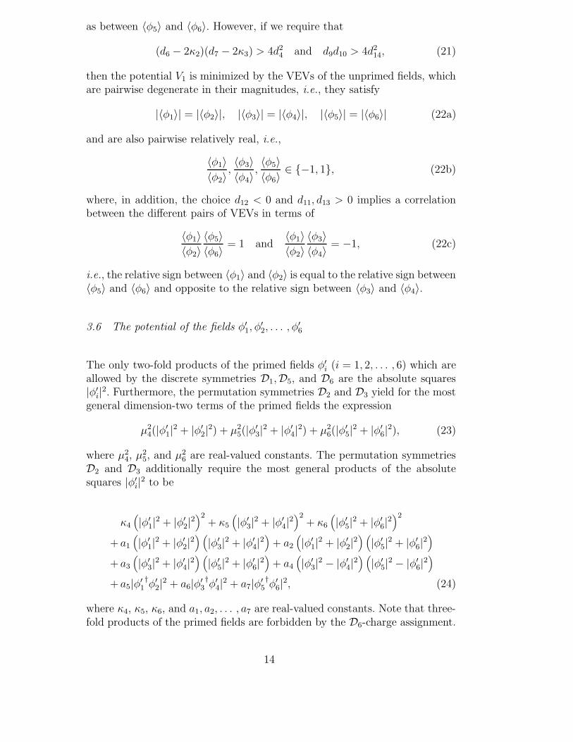
as between 〈φ5〉 and 〈φ6〉. However, if we require that

(d6 − 2κ2)(d7 − 2κ3) > 4d24 and d9d10 > 4d2

14, (21)

then the potential V1 is minimized by the VEVs of the unprimed fields, whichare pairwise degenerate in their magnitudes, i.e., they satisfy

|〈φ1〉| = |〈φ2〉|, |〈φ3〉| = |〈φ4〉|, |〈φ5〉| = |〈φ6〉| (22a)

and are also pairwise relatively real, i.e.,

〈φ1〉〈φ2〉 ,

〈φ3〉〈φ4〉 ,

〈φ5〉〈φ6〉 ∈ {−1, 1}, (22b)

where, in addition, the choice d12 < 0 and d11, d13 > 0 implies a correlationbetween the different pairs of VEVs in terms of

〈φ1〉〈φ2〉

〈φ5〉〈φ6〉 = 1 and

〈φ1〉〈φ2〉

〈φ3〉〈φ4〉 = −1, (22c)

i.e., the relative sign between 〈φ1〉 and 〈φ2〉 is equal to the relative sign between〈φ5〉 and 〈φ6〉 and opposite to the relative sign between 〈φ3〉 and 〈φ4〉.

3.6 The potential of the fields φ′1, φ′2, . . . , φ′6

The only two-fold products of the primed fields φ′i (i = 1, 2, . . . , 6) which areallowed by the discrete symmetries D1,D5, and D6 are the absolute squares|φ′i|2. Furthermore, the permutation symmetries D2 and D3 yield for the mostgeneral dimension-two terms of the primed fields the expression

µ24(|φ′1|2 + |φ′2|2) + µ2

5(|φ′3|2 + |φ′4|2) + µ26(|φ′5|2 + |φ′6|2), (23)

where µ24, µ2

5, and µ26 are real-valued constants. The permutation symmetries

D2 and D3 additionally require the most general products of the absolutesquares |φ′i|2 to be

κ4

(|φ′1|2 + |φ′2|2

)2+ κ5

(|φ′3|2 + |φ′4|2

)2+ κ6

(|φ′5|2 + |φ′6|2

)2

+ a1

(|φ′1|2 + |φ′2|2

) (|φ′3|2 + |φ′4|2

)+ a2

(|φ′1|2 + |φ′2|2

) (|φ′5|2 + |φ′6|2

)+ a3

(|φ′3|2 + |φ′4|2

) (|φ′5|2 + |φ′6|2

)+ a4

(|φ′3|2 − |φ′4|2

) (|φ′5|2 − |φ′6|2

)+ a5|φ′1†φ′2|2 + a6|φ′3†φ′4|2 + a7|φ′5†φ′6|2, (24)

where κ4, κ5, κ6, and a1, a2, . . . , a7 are real-valued constants. Note that three-fold products of the primed fields are forbidden by the D6-charge assignment.

14

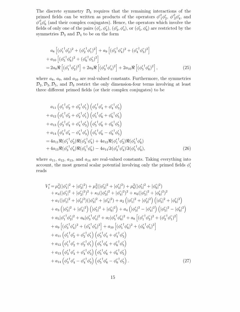
The discrete symmetry D6 requires that the remaining interactions of theprimed fields can be written as products of the operators φ′†1φ

′2, φ′†3φ

′4, and

φ′†5φ′6 (and their complex conjugates). Hence, the operators which involve the

fields of only one of the pairs (φ′1, φ′2), (φ′3, φ

′4), or (φ′5, φ

′6) are restricted by the

symmetries D3 and D4 to be on the form

a8

[(φ′1

†φ′2)

2 + (φ′2†φ′1)

2]+ a9

[(φ′3

†φ′4)

2 + (φ′4†φ′3)

2]

+ a10

[(φ′5

†φ′6)

2 + (φ′6†φ′5)

2]

=2a8<[(φ′1

†φ′2)

2]+ 2a9<

[(φ′3

†φ′4)

2]+ 2a10<

[(φ′5

†φ′6)

2], (25)

where a8, a9, and a10 are real-valued constants. Furthermore, the symmetriesD2,D3,D5, and D6 restrict the only dimension-four terms involving at leastthree different primed fields (or their complex conjugates) to be

a11

(φ′1

†φ′2 + φ′2

†φ′1) (

φ′3†φ′4 + φ′4

†φ′3)

+ a12

(φ′1

†φ′2 + φ′2

†φ′1) (

φ′5†φ′6 + φ′6

†φ′5)

+ a13

(φ′3

†φ′4 + φ′4

†φ′3) (

φ′5†φ′6 + φ′6

†φ′5)

+ a14

(φ′3

†φ′4 − φ′4

†φ′3) (

φ′5†φ′6 − φ′6

†φ′5)

=4a11<(φ′1†φ′2)<(φ′3

†φ′4) + 4a12<(φ′1

†φ′2)<(φ′5

†φ′6)

+ 4a13<(φ′3†φ′4)<(φ′5

†φ′6)− 4a14=(φ′3

†φ′4)=(φ′5

†φ′6), (26)

where a11, a12, a13, and a14 are real-valued constants. Taking everything intoaccount, the most general scalar potential involving only the primed fields φ′ireads

V ′1 =µ2

4(|φ′1|2 + |φ′2|2) + µ25(|φ′3|2 + |φ′4|2) + µ2

6(|φ′5|2 + |φ′6|2)+κ4(|φ′1|2 + |φ′2|2)2 + κ5(|φ′3|2 + |φ′4|2)2 + κ6(|φ′5|2 + |φ′6|2)2

+ a1(|φ′1|2 + |φ′2|2)(|φ′3|2 + |φ′4|2) + a2

(|φ′1|2 + |φ′2|2

) (|φ′5|2 + |φ′6|2

)+ a3

(|φ′3|2 + |φ′4|2

) (|φ′5|2 + |φ′6|2

)+ a4

(|φ′3|2 − |φ′4|2

) (|φ′5|2 − |φ′6|2

)+ a5|φ′1†φ′2|2 + a6|φ′3†φ′4|2 + a7|φ′5†φ′6|2 + a8

[(φ′1

†φ′2)

2 + (φ′2†φ′1)

2]

+ a9

[(φ′3

†φ′4)

2 + (φ′4†φ′3)

2]+ a10

[(φ′5

†φ′6)

2 + (φ′6†φ′5)

2]

+ a11

(φ′1

†φ′2 + φ′2

†φ′1) (

φ′3†φ′4 + φ′4

†φ′3)

+ a12

(φ′1

†φ′2 + φ′2

†φ′1) (

φ′5†φ′6 + φ′6

†φ′5)

+ a13

(φ′3

†φ′4 + φ′4

†φ′3) (

φ′5†φ′6 + φ′6

†φ′5)

+ a14

(φ′3

†φ′4 − φ′4

†φ′3) (

φ′5†φ′6 − φ′6

†φ′5). (27)

15

In Eq. (27), we will assume that κ4, κ5, κ6 > 0 and we will choose all othercoupling constants to be negative. As in the discussion of the potential V1,we observe that the first nine terms in Eq. (27) exhibit three accidental U(1)symmetries, which act on the pairs of VEVs (〈φ′1〉, 〈φ′2〉), (〈φ′3〉, 〈φ′4〉), and(〈φ′5〉, 〈φ′6〉), respectively. The rest of the terms in the potential V ′

1 break thesesymmetries and will therefore determine the vacuum alignment mechanism ofthe fields. If we, in analogy to the potential V1, require that

(a6 − 2κ5)(a7 − 2κ6) > 4a24 and a9a10 > 4a2

14, (28)

then the potential V ′1 is minimized by the VEVs of the primed fields, which

are pairwise degenerate in their magnitudes, i.e., they satisfy

|〈φ′1〉| = |〈φ′2〉|, |〈φ′3〉| = |〈φ′4〉|, |〈φ′5〉| = |〈φ′6〉| (29a)

and are also pairwise relatively real obeying

〈φ′1〉〈φ′2〉

=〈φ′3〉〈φ′4〉

=〈φ′5〉〈φ′6〉

∈ {−1, 1}. (29b)

Note that in Eq. (29b) the pairs of the VEVs (〈φ′1〉, 〈φ′2〉), (〈φ′3〉, 〈φ′4〉), and(〈φ′5〉, 〈φ′6〉) have the same relative phase, i.e., the VEVs in the pairs are eitherall oriented parallel or all oriented antiparallel.

3.7 Mixing among the fields φ′1, φ′2, . . . , φ′6 and φ1, φ2, . . . , φ6

The discrete symmetry D6 requires all renormalizable terms mixing the primedfields φ′i or φ′i

† (i = 1, 2, . . . , 6) with the unprimed fields φj or φ†j (j =1, 2, . . . , 6) to have an even mass dimension. Taking the combinations inEq. (7) and the product φ†3,4φ3,4 into account (which are all D6-singlets), weobtain that the D1-invariant operator products, which mix the fields φ′i andφj, must be of the types

φ′†i1φ′i2φ

†1,2φ1,2 , φ′†i1φ

′i2φ

†3,4φ3,4 , φ′†i1φ

′i2φ

†5,6φ5,6 , (30)

where i1, i2 = 1, 2, . . . , 6. The symmetry D4, which acts only on the unprimedfields, requires the combinations in Eq. (30) to be on the form φ′†i1φ

′i2|φ†j|2,

where j = 1, 2, . . . , 6. Next, the symmetries D5 and D6 imply that the opera-tors in Eq. (30) are all in fact ∼ |φ′i|2|φj|2. As a result, the most general renor-malizable interactions of the fields φ′1, φ

′2, . . . , φ′6 with the fields φ1, φ2, . . . , φ6

are

16

V2 =(|φ′1|2 + |φ′2|2

)×[b1

(|φ1|2 + |φ2|2

)+ b2

(|φ3|2 + |φ4|2

)+ b3

(|φ5|2 + |φ6|2

)]+ b4

(|φ′1|2 − |φ′2|2

) (|φ1|2 − |φ2|2

)+(|φ′3|2 + |φ′4|2

)×[b5

(|φ1|2 + |φ2|2

)+ b6

(|φ3|2 + |φ4|2

)+ b7

(|φ5|2 + |φ6|2

)]+(|φ′3|2 − |φ′4|2

) [b8

(|φ3|2 − |φ4|2

)+ b9

(|φ5|2 − |φ6|2

)]+(|φ′5|2 + |φ′6|2

)×[b10

(|φ1|2 + |φ2|2

)+ b11

(|φ3|2 + |φ4|2

)+ b12

(|φ5|2 + |φ6|2

)]+(|φ′5|2 − |φ′6|2

) [b13

(|φ3|2 − |φ4|2

)+ b14

(|φ5|2 − |φ6|2

)], (31)

where b1, b2, . . . , b14 are real-valued constants. In Eq. (31), we will assume allcoupling constants to be negative.

In order to recover the (same) vacuum alignment mechanism that is operativefor the potentials V1, V ′

1 , and V7,8 also for the full SM singlet scalar potentialV ≡ V1 + V ′

1 + V2 + V7,8, we will have to ensure that the mixed terms inthe potential V2 do not induce a splitting between the pairwise degeneratemagnitudes of the VEVs. If we require the coupling constants in the potentialsV1, V ′

1 , and V2 to fulfill

(a5 − 2κ4)(d5 − 2κ1) > 4b24,

(a6 − 2κ5)(d6 − 2κ2) > 4b28, (a6 − 2κ5)(d7 − 2κ3) > 4b2

9,

(a7 − 2κ6)(d6 − 2κ2) > 4b213, (a7 − 2κ6)(d7 − 2κ3) > 4b2

14, (32)

then the total multi-scalar potential V is indeed minimized by the VEVs ofEqs. (12), (22), and (29).

We will suppose that all of the SM singlet scalar fields break the flavor sym-metries by acquiring their VEVs at a high mass scale (somewhat below thefundamental mass scale M1), and thereby, giving rise to a small expansionparameter

ε ' 〈φi〉M1

' 〈φ′j〉M1

' 〈θ〉M1

' 10−1, (33)

where i = 1, 2, . . . , 10 and j = 1, 2, . . . , 6. Such small hierarchies can arisefrom large hierarchies in supersymmetric theories when the scalar fields acquiretheir VEVs along a “D-flat” direction [62, 63].

In the next two sections, Secs. 4 and 5, we will discuss the (effective) Yukawainteractions of the leptons that will lead to the mass matrix textures of the

17

leptons, and eventually, to the masses and mixings of them, which will bediscussed in Secs. 6 and 7.

4 Yukawa interactions of the charged leptons

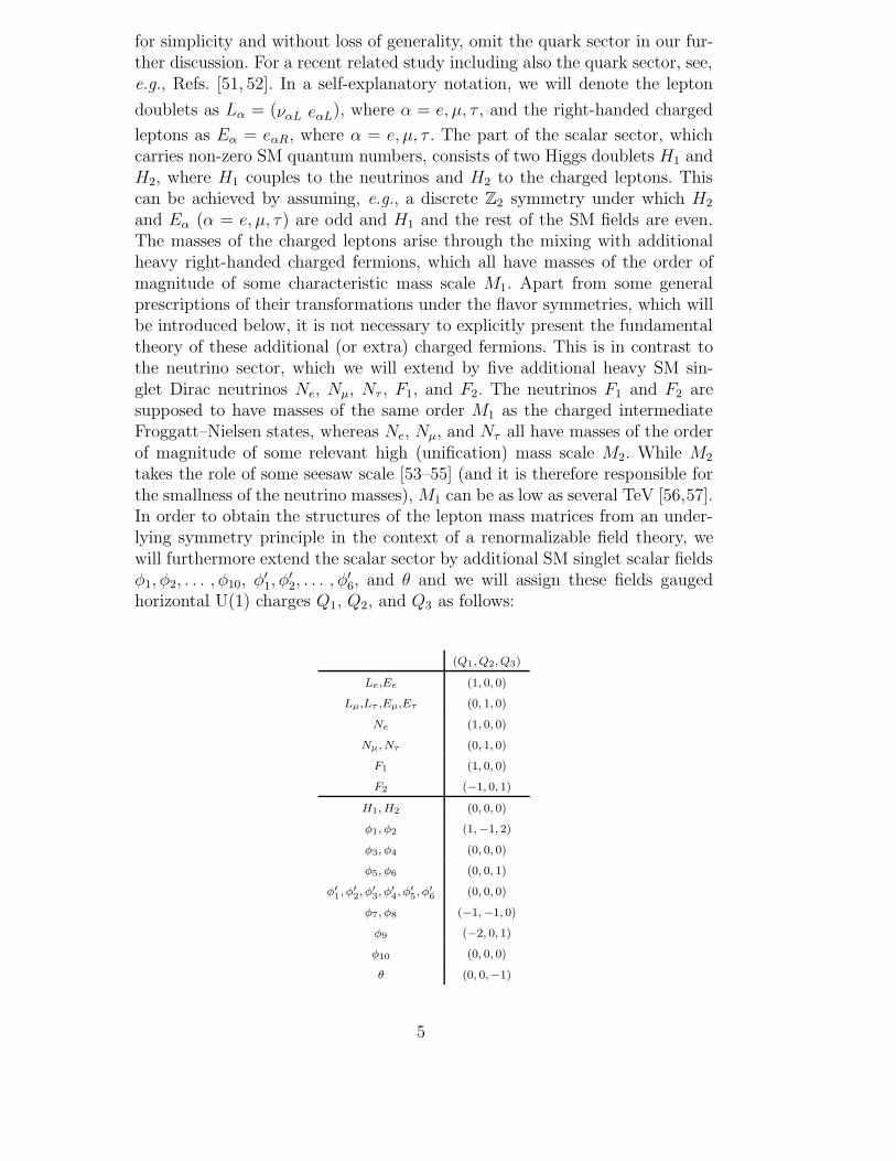
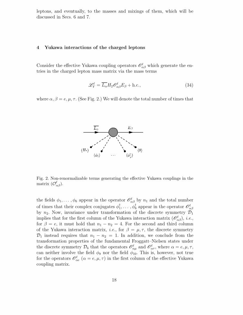
Consider the effective Yukawa coupling operators O`αβ which generate the en-

tries in the charged lepton mass matrix via the mass terms

L `Y = LαH2O

`αβEβ + h.c., (34)

where α, β = e, µ, τ . (See Fig. 2.) We will denote the total number of times that

L� E�

hH2ih�ii � � � h�0

jih�i

Fig. 2. Non-renormalizable terms generating the effective Yukawa couplings in thematrix (O`

αβ).

the fields φ1, . . . , φ6 appear in the operator O`αβ by n1 and the total number

of times that their complex conjugates φ†1, . . . , φ†6 appear in the operator O`αβ

by n2. Now, invariance under transformation of the discrete symmetry D1

implies that for the first column of the Yukawa interaction matrix (O`αβ), i.e.,

for β = e, it must hold that n1 − n2 = 4. For the second and third columnof the Yukawa interaction matrix, i.e., for β = µ, τ , the discrete symmetryD1 instead requires that n1 − n2 = 1. In addition, we conclude from thetransformation properties of the fundamental Froggatt–Nielsen states underthe discrete symmetry D6 that the operators O`

αµ and O`ατ , where α = e, µ, τ ,

can neither involve the field φ9 nor the field φ10. This is, however, not truefor the operators O`

αe (α = e, µ, τ) in the first column of the effective Yukawacoupling matrix.

18

4.1 The first row and column of the charged lepton mass matrix

Invariance under transformations of the U(1) symmetries requires the U(1)charges of the entries O`

eµ and O`eτ in the first row of the effective Yukawa

coupling matrix (O`αβ) to be (1,−1, 0). Since the fields φ9 and φ10 cannot be

involved in the generation of the e-µ- and e-τ -elements of the charged leptonmass matrix, the U(1) charge assignment immediately implies that any massoperator giving rise to these e-µ- and e-τ -elements must involve the term∼ φ1,2θ

2/(M1)3. Next, the symmetries D5 and D6 yield to leading order for

the operators O`eµ and O`

eτ the two possible terms ∼ φ1φ′1θ

2/(M1)4 and ∼

φ2φ′2θ

2/(M1)4. In conjuction with the requirement n1− n2 = 1, the symmetry

D6 implies that any further operators contributing to the operator O`eµ or

O`eτ must have at least two powers of mass dimension more than the terms

φ1φ′1θ

2/(M1)4 and φ2φ

′2θ

2/(M1)4. We will therefore neglect these additional

operators.

From the transformation properties of the right-handed electron Ee and thefundamental Froggatt–Nielsen states under transformations of the discretesymmetries D1 and D6, we conclude that the operators O`

ee, O`µe, and O`

τe inthe first column of the effective Yukawa coupling matrix must involve at leasta four-fold product of fields taken from the set {φ1, φ2, φ3, φ4, φ5, φ6} times afield taken from the set {φ9, φ10}. The lowest-dimensional contribution to theoperator O`

ee, which has the charge structure (0, 0, 0) and yields an invariantunder transformation of all the discrete symmetries, is given by

O`ee =

φ10

(M1)5

[(φ3)

4 + (φ4)4]. (35)

The remaining operators O`µe and O`

τe have a mass dimension that is greaterthan or equal to the mass dimension of the terms in Eq. (35). However, theeffects of these terms on the leptonic mixing angles will turn out to be neg-ligible in comparison with the contributions coming from other entries of thecharged lepton mass matrix.

In total, the first row of the effective Yukawa coupling matrix of the chargedleptons, which is consistent with all of the discrete symmetries, is to leadingorder

(O`eα) =

(A1 [(φ3)

4 + (φ4)4] B1 [φ1φ

′1 − φ2φ

′2] B1 [φ1φ

′1 + φ2φ

′2]

). (36a)

Here the dimensionful coefficients A1 and B1 are given by

19

A1 = Y `a

φ10

(M1)5, (36b)

B1 = Y `b

θ2

(M1)4, (36c)

where the quantities Y `a and Y `

b are arbitrary order unity coefficients and M1

is the high mass scale of the intermediate Froggatt–Nielsen states. Note thatat the level of the fundamental theory, the permutation symmetry D4, whichinterchanges the second and third generations of the leptons, is also propagatedto the heavy Froggatt–Nielsen states. This establishes a degeneracy of theassociated Yukawa couplings and the explicit masses of these states, whichis then translated into a degeneracy of the corresponding effective Yukawacouplings of the low-energy theory.

4.2 The 2-3-submatrix of the charged lepton mass matrix

In the 2-3-submatrix of the charged lepton mass matrix, the U(1) chargesof the operators O`

αβ (α, β = µ, τ) must be (0, 0, 0). The lowest dimensionaloperators which fulfill this condition as well as the constraint n1 − n2 = 1are proportional to φ3,4/M1 or φ5,6θ/(M1)

2. Furthermore, invariance undertransformation of the discrete symmetries D5 and D6 implies that the lowestdimensional operators O`

αβ in the 2-3-submatrix with n1 − n2 = 1 are of thetypes

φ′3φ3

(M1)2,

φ′4φ4

(M1)2,

φ′5φ5θ

(M1)3,

φ′6φ6θ

(M1)3. (37)

Thus, the most general 2-3-submatrix of the matrix (O`αβ), which involves only

these combinations and is invariant under transformations of the remainingdiscrete symmetries, is found to be

C(φ′3φ3 − φ′4φ4) + D(φ′5φ5 − φ′6φ6) 0

0 C(φ′3φ3 + φ′4φ4) + D(φ′5φ5 + φ′6φ6)

.

(38a)

Here the dimensionful coefficients C and D are given by

C = Y `c

1

(M1)2, (38b)

D = Y `d

θ

(M1)3, (38c)

20

where the quantities Y `c and Y `

d are arbitrary order unity coefficients. Actually,contributions to the next-leading operators O`

µτ and O`τµ are, e.g., given by

µ-τ :1

(M1)4(a1φ7φ

†8 + a2φ8φ

†7)(φ3 + φ4)φ

′3, (39a)

τ -µ :1

(M1)4(a2φ7φ

†8 + a1φ8φ

†7)(φ3 − φ4)φ

′3, (39b)

where a1 and a2 are some complex-valued constants. Note that the terms inEqs. (39) carry only one unit of mass dimension more than, e.g., the termφ′5φ5θ/(M1)

3 in Eq. (38a). When diagonalizing the mass matrix, however, itwill turn out that the associated corrections to the leptonic mixing parametersand the lepton masses are in fact negligible.

4.3 The charged lepton mass matrix

Combining the results of Secs. 4.1 and 4.2, the leading order effective Yukawacoupling matrix of the charged leptons is

(O`αβ) =

(A1

[(φ3)4 + (φ4)4

]B1

[φ1φ′

1 − φ2φ′2

]B1

[φ1φ′

1 + φ2φ′2

]0 C(φ′

3φ3 − φ′4φ4) + D(φ′

5φ5 − φ′6φ6) 0

0 0 C(φ′3φ3 + φ′

4φ4) + D(φ′5φ5 + φ′

6φ6)

),

(40)

where the dimensionful couplings A1, B1, C, and D are given in Eqs. (36b),(36c), (38b), and (38c), respectively. Inserting the VEVs in Eqs. (29) and (22)into the corresponding operators of the matrix (O`

αβ), we observe that, due tothe vacuum alignment mechanism of the SM singlet scalar fields, in some ofthe entries of the matrix ((M`)αβ), the spontaneously generated effective massterms of a given order exactly cancel, whereas in other entries they do not.Furthermore, the vacuum alignment mechanism correlates these cancellationsin the different entries of the matrix ((M`)αβ) in such a way that after SSB thecharged lepton mass matrix M` can be of the two possible asymmetric forms

M` ' mexpτ

ε3 ε2 ε4

ε3 ε ε2

ε3 ε2 1

(41)

21

and

M` ' mexpτ

ε3 ε4 ε2

ε3 1 ε2

ε3 ε2 ε

, (42)

where we have also introduced the appropriate orders of magnitude for thematrix elements (M`)µe and (M`)τe as well as for the “phenomenological” (incontrast to exact) texture zeros arising in Eqs. (36a) and (38a). Here mexp

τ isthe (experimental) tau mass. Note that a permutation of the second and thirdgenerations Lµ ↔ Lτ , Eµ ↔ Eτ leads from one solution to another. Let usconsider the first one for our remaining discussion.

5 Yukawa interactions of the neutrinos

Consider the effective Yukawa coupling operators Oναβ which generate the en-

tries in the neutrino mass matrix Mν via the mass terms

L νY = Lc

α

H21

M2Oν

αβLβ + h.c., (43)

where α, β = e, µ, τ and M2 is the relevant high mass scale which is responsiblefor the smallness of the neutrino masses in comparison with the charged leptonmasses. Since the SM singlet neutrinos as well as the Higgs doublets are D1-singlets, the presence of the fields φ1, . . . , φ6 (which transform non-triviallyunder the discrete symmetry D1) in the operators Oν

αβ is forbidden. Hence,the only scalar fields that can be involved in the leading order operators Oν

αβ

are φ7, φ8, φ9, φ10, and θ.

5.1 Effective Yukawa interactions of the neutrinos

The operators Oνµµ, O

νµτ , O

ντµ, and Oν

ττ must have the U(1) charge structure(0,−2, 0). An example of the lowest dimensional operators which achieve thisis

∼ φ9φ10θ

(M1)5

[(φ†7)

2 + (φ†8)2]. (44)

22

Since the U(1) charge structure of the entry Oνee is (−2, 0, 0), the operator Oν

ee

is to leading order

Oνee = Y ν

a

φ9φ10θ

(M1)3, (45)

where Y νa is an arbitrary order unity coefficient. Note that the operators of the

type in Eq. (44) carry two units of mass dimension more than the operatorOν

ee.

The operators Oνeµ and Oν

eτ (as well as Oνµe and Oν

τe) must have the U(1) chargestructure (−1,−1, 0). Therefore, the lowest dimensional terms which con-tribute to these operators are ∼ φ7/M1 and ∼ φ8/M1. The symmetries D2,D3,and D4 then yield to leading order Oν

eµ = Y νb φ7/M1 and Oν

eτ = Y νb φ8/M1,

where Y νb is an arbitrary order unity coefficient. Note that the operator Oν

ee

in Eq. (45) carries two units of mass dimension more than the operatorsOν

eµ ∼ φ7/M1 and Oνeτ ∼ φ8/M1. We will therefore not in detail consider

the structure of the highly suppressed terms that appear in the 2-3-submatrixof the neutrino mass matrix as the operator given in Eq. (44).

In total, the most general effective Yukawa coupling matrix of the neutrinos(Oν

αβ) that is consistent with the symmetries of our model is to leading ordergiven by

(Oναβ) =

A2 B2 B3

B2 0 0

B3 0 0

. (46)

Here the dimensionful coefficients A2, B2, and B3 are given by

A2 = Y νa

φ9φ10θ

(M1)3, (47a)

B2 = Y νb

φ7

M1, (47b)

B3 = Y νb

φ8

M1, (47c)

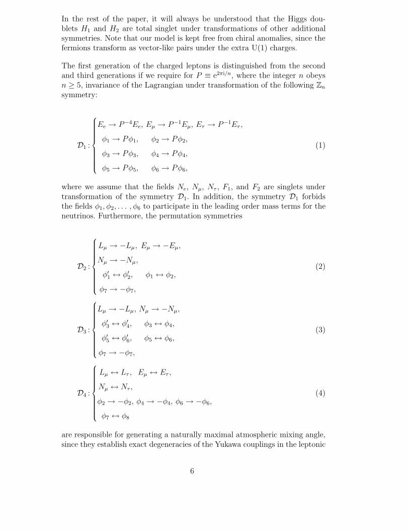
where the quantity Y νb is an order unity coefficient. The leading order tree level

realizations of the higher-dimensional operators, which generate the neutrinomasses, are shown in Figs. 3 and 4. Note that the coefficients B2 and B3

contain the same Yukawa coupling constant Y νb . Furthermore, we point out

that the texture zeros in the 2-3-submatrix of the effective neutrino Yukawamatrix should be understood as “phenomenological” ones, since they actuallyrepresent highly suppressed operators carrying two units of mass dimensionmore than the entry Oν

ee.

23

Lce F c

1F c

1 N� N� L�

H1

��H1

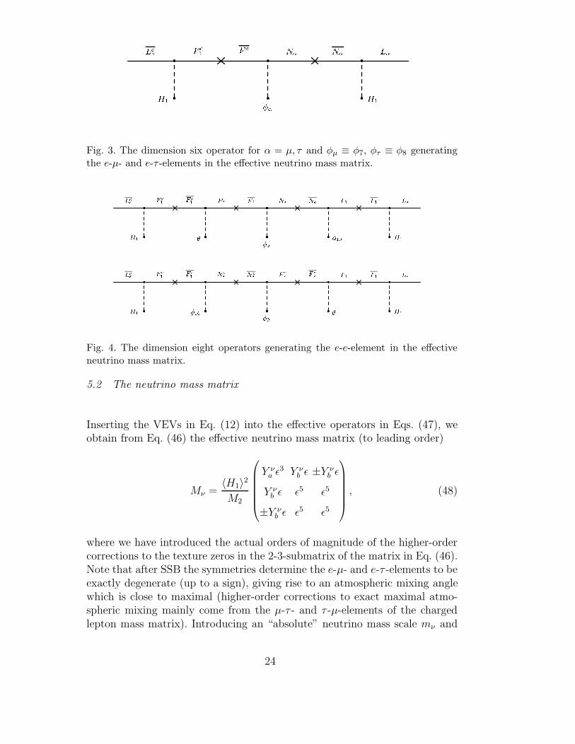
Fig. 3. The dimension six operator for α = µ, τ and φµ ≡ φ7, φτ ≡ φ8 generatingthe e-µ- and e-τ -elements in the effective neutrino mass matrix.

Lc

eF c

1F c

1 F2 F2 Ne Ne F1 F1 Le

H1 ��9

�10 H1

Lc

eF c

1F c

1 Nc

e Nc

eF c

2F c

2 F1 F1 Le

H1 �10�9

� H1

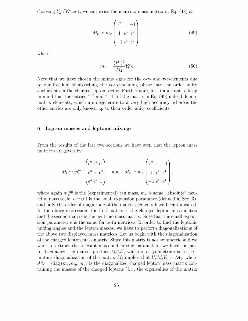
Fig. 4. The dimension eight operators generating the e-e-element in the effectiveneutrino mass matrix.

5.2 The neutrino mass matrix

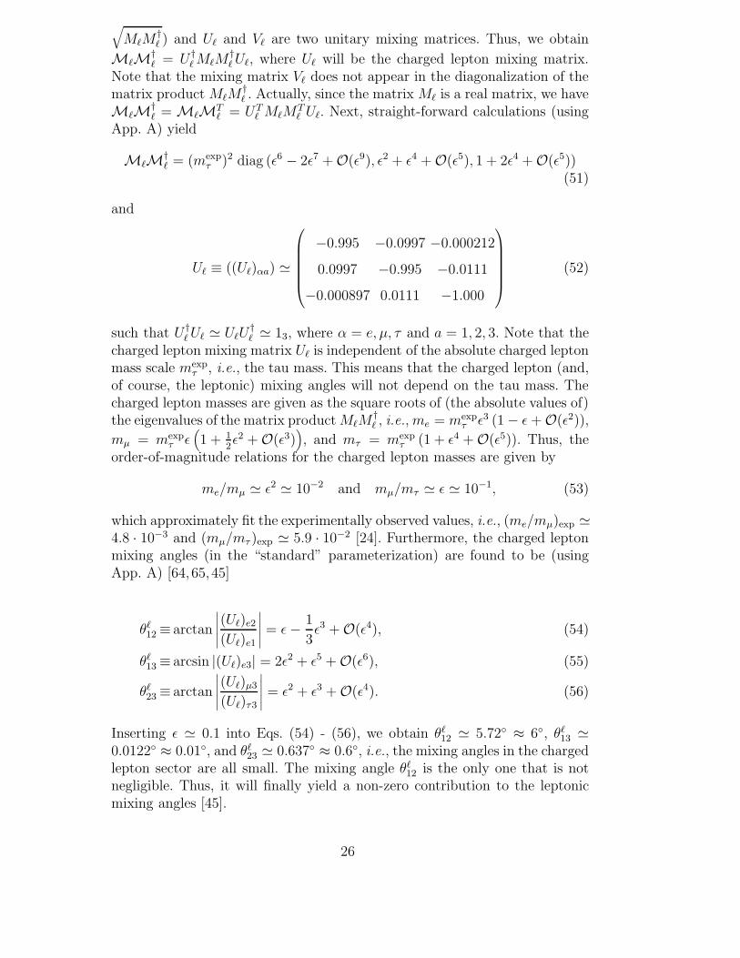
Inserting the VEVs in Eq. (12) into the effective operators in Eqs. (47), weobtain from Eq. (46) the effective neutrino mass matrix (to leading order)

Mν =〈H1〉2M2

Y νa ε3 Y ν

b ε ±Y νb ε

Y νb ε ε5 ε5

±Y νb ε ε5 ε5

, (48)

where we have introduced the actual orders of magnitude of the higher-ordercorrections to the texture zeros in the 2-3-submatrix of the matrix in Eq. (46).Note that after SSB the symmetries determine the e-µ- and e-τ -elements to beexactly degenerate (up to a sign), giving rise to an atmospheric mixing anglewhich is close to maximal (higher-order corrections to exact maximal atmo-spheric mixing mainly come from the µ-τ - and τ -µ-elements of the chargedlepton mass matrix). Introducing an “absolute” neutrino mass scale mν and

24

choosing Y νa /Y ν

b ' 1, we can write the neutrino mass matrix in Eq. (48) as

Mν ' mν

ε2 1 −1

1 ε4 ε4

−1 ε4 ε4

, (49)

where

mν =〈H1〉2M2

Y νb ε. (50)

Note that we have chosen the minus signs for the e-τ - and τ -e-elements dueto our freedom of absorbing the corresponding phase into the order unitycoefficients in the charged lepton sector. Furthermore, it is important to keepin mind that the entries “1” and “−1” of the matrix in Eq. (49) indeed denotematrix elements, which are degenerate to a very high accuracy, whereas theother entries are only known up to their order unity coefficients.

6 Lepton masses and leptonic mixings

From the results of the last two sections we have seen that the lepton massmatrices are given by

M` ' mexpτ

ε3 ε2 ε4

ε3 ε ε2

ε3 ε2 1

and Mν ' mν

ε2 1 −1

1 ε4 ε4

−1 ε4 ε4

,

where again mexpτ is the (experimental) tau mass, mν is some “absolute” neu-

trino mass scale, ε ' 0.1 is the small expansion parameter (defined in Sec. 3),and only the order of magnitude of the matrix elements have been indicated.In the above expression, the first matrix is the charged lepton mass matrixand the second matrix is the neutrino mass matrix. Note that the small expan-sion parameter ε is the same for both matrices. In order to find the leptonicmixing angles and the lepton masses, we have to perform diagonalizations ofthe above two displayed mass matrices. Let us begin with the diagonalizationof the charged lepton mass matrix. Since this matrix is not symmetric and wewant to extract the relevant mass and mixing parameters, we have, in fact,to diagonalize the matrix product M`M

†` , which is a symmetric matrix. Bi-

unitary diagonalization of the matrix M` implies that U †` M`V` = M`, where

M` = diag (me, mµ, mτ ) is the diagonalized charged lepton mass matrix con-taining the masses of the charged leptons (i.e., the eigenvalues of the matrix

25

√M`M

†` ) and U` and V` are two unitary mixing matrices. Thus, we obtain

M`M†` = U †

` M`M†` U`, where U` will be the charged lepton mixing matrix.

Note that the mixing matrix V` does not appear in the diagonalization of thematrix product M`M

†` . Actually, since the matrix M` is a real matrix, we have

M`M†` = M`MT

` = UT` M`M

T` U`. Next, straight-forward calculations (using

App. A) yield

M`M†` = (mexp

τ )2 diag (ε6 − 2ε7 +O(ε9), ε2 + ε4 +O(ε5), 1 + 2ε4 +O(ε5))(51)

and

U` ≡ ((U`)αa) '

−0.995 −0.0997 −0.000212

0.0997 −0.995 −0.0111

−0.000897 0.0111 −1.000

(52)

such that U †` U` ' U`U

†` ' 13, where α = e, µ, τ and a = 1, 2, 3. Note that the

charged lepton mixing matrix U` is independent of the absolute charged leptonmass scale mexp

τ , i.e., the tau mass. This means that the charged lepton (and,of course, the leptonic) mixing angles will not depend on the tau mass. Thecharged lepton masses are given as the square roots of (the absolute values of)the eigenvalues of the matrix product M`M

†` , i.e., me = mexp

τ ε3 (1− ε +O(ε2)),

mµ = mexpτ ε

(1 + 1

2ε2 +O(ε3)

), and mτ = mexp

τ (1 + ε4 +O(ε5)). Thus, theorder-of-magnitude relations for the charged lepton masses are given by

me/mµ ' ε2 ' 10−2 and mµ/mτ ' ε ' 10−1, (53)

which approximately fit the experimentally observed values, i.e., (me/mµ)exp '4.8 · 10−3 and (mµ/mτ )exp ' 5.9 · 10−2 [24]. Furthermore, the charged leptonmixing angles (in the “standard” parameterization) are found to be (usingApp. A) [64, 65, 45]

θ`12≡ arctan

∣∣∣∣∣(U`)e2

(U`)e1

∣∣∣∣∣ = ε− 1

3ε3 +O(ε4), (54)

θ`13≡ arcsin |(U`)e3| = 2ε2 + ε5 +O(ε6), (55)

θ`23≡ arctan

∣∣∣∣∣(U`)µ3

(U`)τ3

∣∣∣∣∣ = ε2 + ε3 +O(ε4). (56)

Inserting ε ' 0.1 into Eqs. (54) - (56), we obtain θ`12 ' 5.72◦ ≈ 6◦, θ`

13 '0.0122◦ ≈ 0.01◦, and θ`

23 ' 0.637◦ ≈ 0.6◦, i.e., the mixing angles in the chargedlepton sector are all small. The mixing angle θ`

12 is the only one that is notnegligible. Thus, it will finally yield a non-zero contribution to the leptonicmixing angles [45].

26

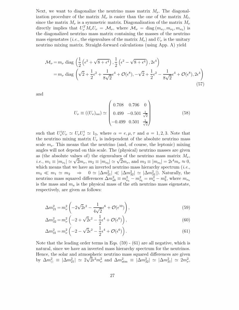
Next, we want to diagonalize the neutrino mass matrix Mν . The diagonal-ization procedure of the matrix Mν is easier than the one of the matrix M`,since the matrix Mν is a symmetric matrix. Diagonalization of the matrix Mν

directly implies that UTν MνUν = Mν , where Mν = diag (mν1, mν2 , mν3) is

the diagonalized neutrino mass matrix containing the masses of the neutrinomass eigenstates (i.e., the eigenvalues of the matrix Mν) and Uν is the unitaryneutrino mixing matrix. Straight-forward calculations (using App. A) yield

Mν =mν diag(

1

2

(ε2 +

√8 + ε4

),1

2

(ε2 −

√8 + ε4

), 2ε4

)

=mν diag

(√2 +

1

2ε2 +

1

8√

2ε4 +O(ε8),−

√2 +

1

2ε2 − 1

8√

2ε4 +O(ε8), 2ε4

)

(57)

and

Uν ≡ ((Uν)αa) '

0.708 0.706 0

0.499 −0.501 1√2

−0.499 0.501 1√2

(58)

such that U †νUν ' UνU

†ν ' 13, where α = e, µ, τ and a = 1, 2, 3. Note that

the neutrino mixing matrix Uν is independent of the absolute neutrino massscale mν . This means that the neutrino (and, of course, the leptonic) mixingangles will not depend on this scale. The (physical) neutrino masses are givenas (the absolute values of) the eigenvalues of the neutrino mass matrix Mν ,i.e., m1 ≡ |mν1| '

√2mν , m2 ≡ |mν2| '

√2mν , and m3 ≡ |mν3| = 2ε4mν ≈ 0,

which means that we have an inverted neutrino mass hierarchy spectrum (i.e.,m3 � m1 ' m2 ⇒ 0 ' |∆m2

21| � |∆m232| ' |∆m2

31|). Naturally, theneutrino mass squared differences ∆m2

ab ≡ m2νa−m2

νb= m2

a −m2b , where mνa

is the mass and ma is the physical mass of the ath neutrino mass eigenstate,respectively, are given as follows:

∆m221 = m2

ν

(−2√

2ε2 − 1

4√

2ε6 +O(ε10)

), (59)

∆m232 = m2

ν

(−2 +

√2ε2 − 1

2ε4 +O(ε6)

), (60)

∆m231 = m2

ν

(−2−

√2ε2 − 1

2ε4 +O(ε6)

). (61)

Note that the leading order terms in Eqs. (59) - (61) are all negative, which isnatural, since we have an inverted mass hierarchy spectrum for the neutrinos.Hence, the solar and atmospheric neutrino mass squared differences are givenby ∆m2

� ≡ |∆m221| ' 2

√2ε2m2

ν and ∆m2atm ≡ |∆m2

32| ' |∆m231| ' 2m2

ν ,

27

respectively. The “experimental” values of these quantities are ∆m2� ' 5.0 ·

10−5 eV2 [23] and ∆m2atm ' 2.5 · 10−3 eV2 [8]. 5 6 Thus, we extract that mν '

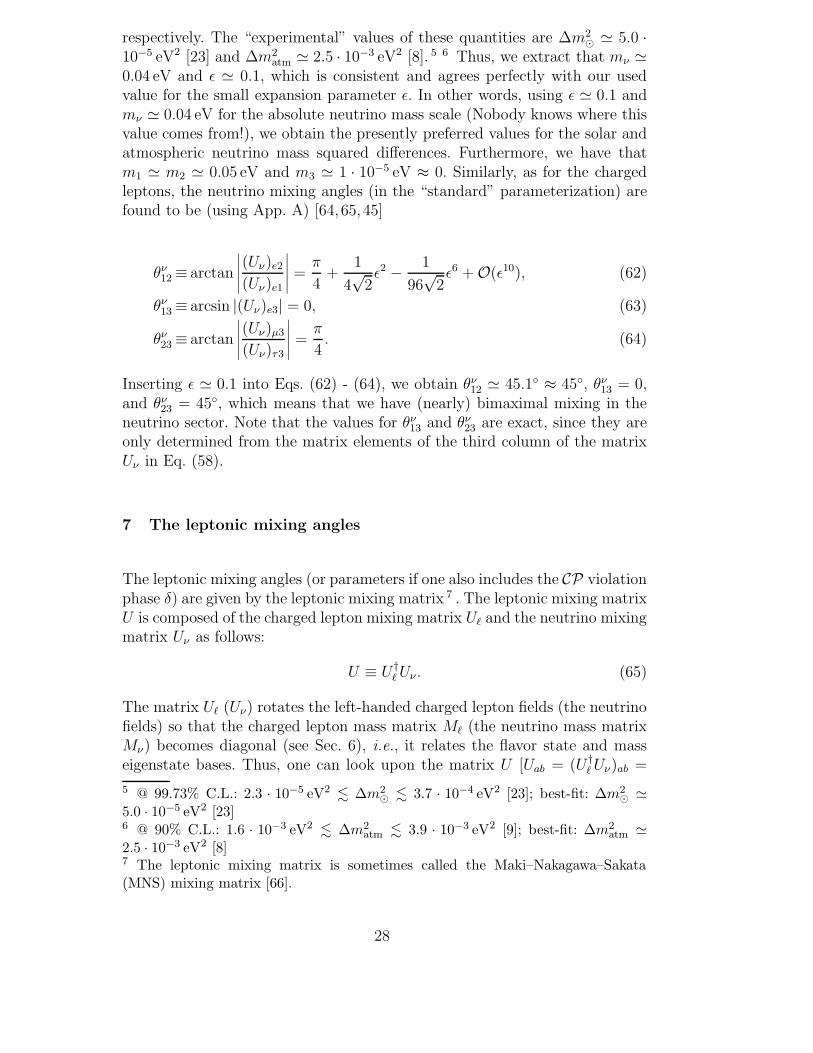
0.04 eV and ε ' 0.1, which is consistent and agrees perfectly with our usedvalue for the small expansion parameter ε. In other words, using ε ' 0.1 andmν ' 0.04 eV for the absolute neutrino mass scale (Nobody knows where thisvalue comes from!), we obtain the presently preferred values for the solar andatmospheric neutrino mass squared differences. Furthermore, we have thatm1 ' m2 ' 0.05 eV and m3 ' 1 · 10−5 eV ≈ 0. Similarly, as for the chargedleptons, the neutrino mixing angles (in the “standard” parameterization) arefound to be (using App. A) [64, 65, 45]

θν12≡ arctan

∣∣∣∣∣(Uν)e2

(Uν)e1

∣∣∣∣∣ = π

4+

1

4√

2ε2 − 1

96√

2ε6 +O(ε10), (62)

θν13≡ arcsin |(Uν)e3| = 0, (63)

θν23≡ arctan

∣∣∣∣∣(Uν)µ3

(Uν)τ3

∣∣∣∣∣ = π

4. (64)

Inserting ε ' 0.1 into Eqs. (62) - (64), we obtain θν12 ' 45.1◦ ≈ 45◦, θν

13 = 0,and θν

23 = 45◦, which means that we have (nearly) bimaximal mixing in theneutrino sector. Note that the values for θν

13 and θν23 are exact, since they are

only determined from the matrix elements of the third column of the matrixUν in Eq. (58).

7 The leptonic mixing angles

The leptonic mixing angles (or parameters if one also includes the CP violationphase δ) are given by the leptonic mixing matrix 7 . The leptonic mixing matrixU is composed of the charged lepton mixing matrix U` and the neutrino mixingmatrix Uν as follows:

U ≡ U †` Uν . (65)

The matrix U` (Uν) rotates the left-handed charged lepton fields (the neutrinofields) so that the charged lepton mass matrix M` (the neutrino mass matrixMν) becomes diagonal (see Sec. 6), i.e., it relates the flavor state and masseigenstate bases. Thus, one can look upon the matrix U [Uab = (U †

` Uν)ab =

5 @ 99.73% C.L.: 2.3 · 10−5 eV2 . ∆m2� . 3.7 · 10−4 eV2 [23]; best-fit: ∆m2� '5.0 · 10−5 eV2 [23]6 @ 90% C.L.: 1.6 · 10−3 eV2 . ∆m2

atm . 3.9 · 10−3 eV2 [9]; best-fit: ∆m2atm '

2.5 · 10−3 eV2 [8]7 The leptonic mixing matrix is sometimes called the Maki–Nakagawa–Sakata(MNS) mixing matrix [66].

28

∑α=e,µ,τ(U

†` )aα(Uν)αb =

∑α=e,µ,τ(U`)

∗αa(Uν)αb] as the messenger between the

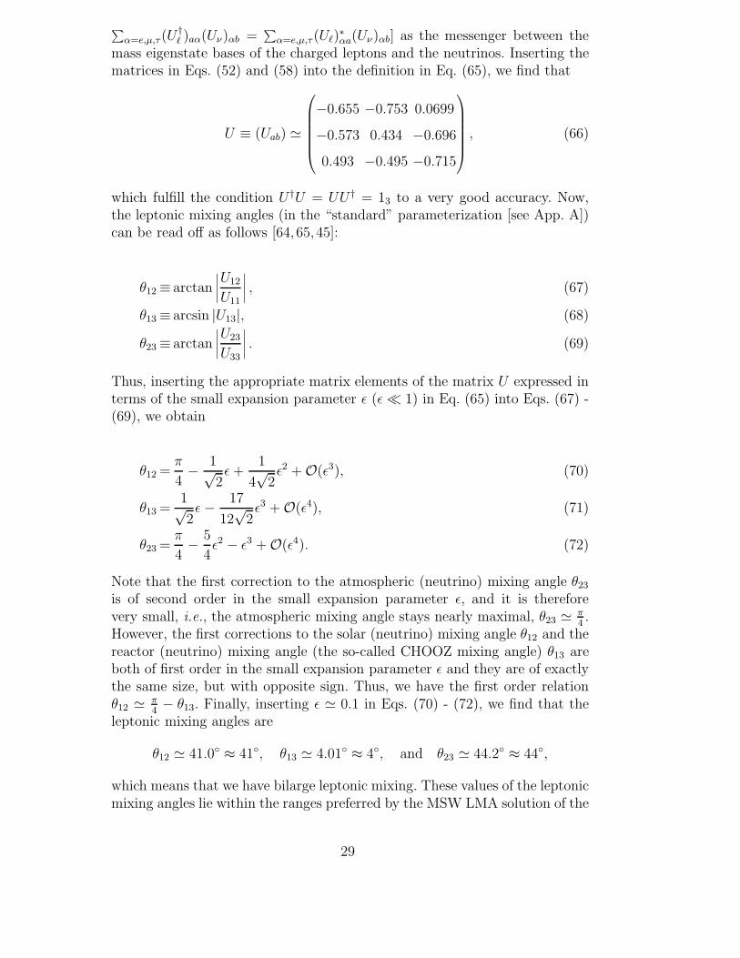
mass eigenstate bases of the charged leptons and the neutrinos. Inserting thematrices in Eqs. (52) and (58) into the definition in Eq. (65), we find that

U ≡ (Uab) '

−0.655 −0.753 0.0699

−0.573 0.434 −0.696

0.493 −0.495 −0.715

, (66)

which fulfill the condition U †U = UU † = 13 to a very good accuracy. Now,the leptonic mixing angles (in the “standard” parameterization [see App. A])can be read off as follows [64, 65, 45]:

θ12≡ arctan

∣∣∣∣U12

U11

∣∣∣∣ , (67)

θ13≡ arcsin |U13|, (68)

θ23≡ arctan

∣∣∣∣U23

U33

∣∣∣∣ . (69)

Thus, inserting the appropriate matrix elements of the matrix U expressed interms of the small expansion parameter ε (ε � 1) in Eq. (65) into Eqs. (67) -(69), we obtain

θ12 =π

4− 1√

2ε +

1

4√

2ε2 +O(ε3), (70)

θ13 =1√2ε− 17

12√

2ε3 +O(ε4), (71)

θ23 =π

4− 5

4ε2 − ε3 +O(ε4). (72)

Note that the first correction to the atmospheric (neutrino) mixing angle θ23

is of second order in the small expansion parameter ε, and it is thereforevery small, i.e., the atmospheric mixing angle stays nearly maximal, θ23 ' π

4.

However, the first corrections to the solar (neutrino) mixing angle θ12 and thereactor (neutrino) mixing angle (the so-called CHOOZ mixing angle) θ13 areboth of first order in the small expansion parameter ε and they are of exactlythe same size, but with opposite sign. Thus, we have the first order relationθ12 ' π

4− θ13. Finally, inserting ε ' 0.1 in Eqs. (70) - (72), we find that the

leptonic mixing angles are

θ12 ' 41.0◦ ≈ 41◦, θ13 ' 4.01◦ ≈ 4◦, and θ23 ' 44.2◦ ≈ 44◦,

which means that we have bilarge leptonic mixing. These values of the leptonicmixing angles lie within the ranges preferred by the MSW LMA solution of the

29

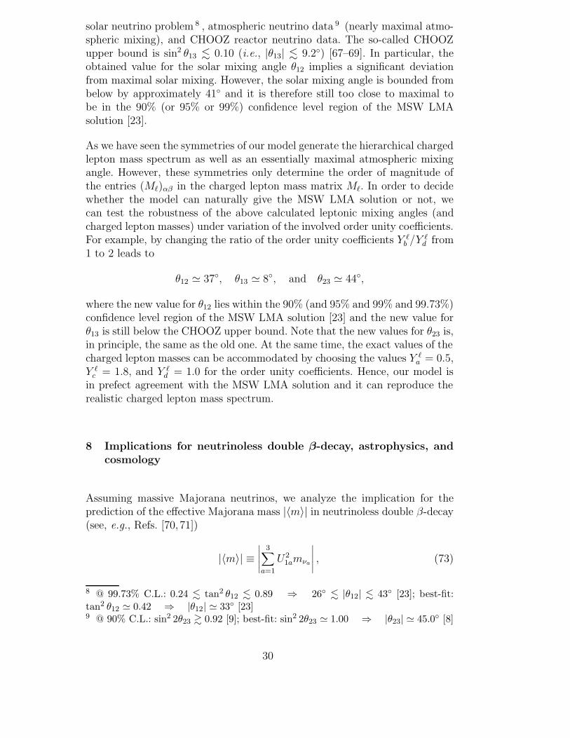
solar neutrino problem 8 , atmospheric neutrino data 9 (nearly maximal atmo-spheric mixing), and CHOOZ reactor neutrino data. The so-called CHOOZupper bound is sin2 θ13 . 0.10 (i.e., |θ13| . 9.2◦) [67–69]. In particular, theobtained value for the solar mixing angle θ12 implies a significant deviationfrom maximal solar mixing. However, the solar mixing angle is bounded frombelow by approximately 41◦ and it is therefore still too close to maximal tobe in the 90% (or 95% or 99%) confidence level region of the MSW LMAsolution [23].

As we have seen the symmetries of our model generate the hierarchical chargedlepton mass spectrum as well as an essentially maximal atmospheric mixingangle. However, these symmetries only determine the order of magnitude ofthe entries (M`)αβ in the charged lepton mass matrix M`. In order to decidewhether the model can naturally give the MSW LMA solution or not, wecan test the robustness of the above calculated leptonic mixing angles (andcharged lepton masses) under variation of the involved order unity coefficients.For example, by changing the ratio of the order unity coefficients Y `

b /Y `d from

1 to 2 leads to

θ12 ' 37◦, θ13 ' 8◦, and θ23 ' 44◦,

where the new value for θ12 lies within the 90% (and 95% and 99% and 99.73%)confidence level region of the MSW LMA solution [23] and the new value forθ13 is still below the CHOOZ upper bound. Note that the new values for θ23 is,in principle, the same as the old one. At the same time, the exact values of thecharged lepton masses can be accommodated by choosing the values Y `

a = 0.5,Y `

c = 1.8, and Y `d = 1.0 for the order unity coefficients. Hence, our model is

in prefect agreement with the MSW LMA solution and it can reproduce therealistic charged lepton mass spectrum.

8 Implications for neutrinoless double β-decay, astrophysics, andcosmology

Assuming massive Majorana neutrinos, we analyze the implication for theprediction of the effective Majorana mass |〈m〉| in neutrinoless double β-decay(see, e.g., Refs. [70, 71])

|〈m〉| ≡∣∣∣∣∣

3∑a=1

U21amνa

∣∣∣∣∣ , (73)

8 @ 99.73% C.L.: 0.24 . tan2 θ12 . 0.89 ⇒ 26◦ . |θ12| . 43◦ [23]; best-fit:tan2 θ12 ' 0.42 ⇒ |θ12| ' 33◦ [23]9 @ 90% C.L.: sin2 2θ23 & 0.92 [9]; best-fit: sin2 2θ23 ' 1.00 ⇒ |θ23| ' 45.0◦ [8]

30

where the U1a’s are first row matrix elements of the leptonic mixing matrix Uand the mνa ’s are the masses of the neutrino mass eigenstates. Inserting theexpressions for the U1a’s and the mνa ’s into Eq. (73), we obtain

|〈m〉|= 1

2mν

[(√8 + ε4 cos 2θ12 + ε2

)cos2 θ13 + 4ε4 sin2 θ13

]

= mν

[√2 cos 2θ12 cos2 θ13 +

1

2cos2 θ13ε

2

+

(1

8√

2cos 2θ12 cos2 θ13 + 2 sin2 θ13

)ε4 +O(ε8)

]

'mν

√2 cos 2θ12 cos2 θ13. (74)

Note that the quantity |〈m〉| becomes equal to zero when θ12 = π4, i.e., when we

have an exactly maximal solar mixing angle. 10 Using mν ' 0.04 eV, θ12 ' 41◦,and θ13 ' 4◦, we find that |〈m〉| ' 0.007 eV, which is consistent with and belowthe phenomenological upper bound |〈m〉| < 0.080 eV [73] for an inverted hier-archical neutrino mass spectrum. Our value for |〈m〉| is also below the exper-imental upper bound obtained from neutrinoless double β-decay experiments(76Ge experiments) by the Heidelberg-Moscow collaboration [|〈m〉| < 0.35 eV(@ 90% C.L.)] [74] and by the IGEX collaboration [|〈m〉| < (0.33÷ 1.35) eV(@ 90% C.L.)] [75, 76]. It would also be below the sensitivity of the plannedneutrinoless double β-decay experiments GENIUS, EXO, MAJORANA, andMOON, which is |〈m〉| ∼ 0.01 eV.

Furthermore, the sum of the neutrino masses

M ≡3∑

a=1

ma, (75)

where the ma’s are the physical masses of the neutrino mass eigenstates, isoften used in astrophysics and cosmology. Inserting the expressions for thema’s into Eq. (75), we obtain

M =mν

(√8 + ε2 + 2ε4

)

=mν

[2√

2 +

(2 +

1

4√

2

)ε4 − 1

128√

2ε8 +O(ε10)

]' 2

√2mν . (76)

Again using mν ' 0.04 eV, we find that M ' 0.1 eV. There exist several upperbounds for this quantity from several different branches of astrophysics and

10 A maximal solar mixing angle could, e.g., imply the presence of a superlightDirac neutrino. For a treatment of naturally light Dirac neutrinos using the seesawmechanism, see, e.g., Ref. [72].

31

cosmology. For example, using the presently best available data from cosmicmicrowave background radiation and large scale structure measurements, wehave the upper bound M < (2.5 ÷ 3) eV (@ 95% C.L.) [77, 78]. Other upperbounds of this quantity come, e.g., from cosmic microwave background radi-ation, galaxy clustering, and Lyman Alpha Forest measurements M < 4.2 eV(@ 95% C.L.) [79] and from the 2dF Galaxy Redshift Survey M < (1.8÷2.2) eV(@ 95% C.L.) [80]. Thus, our value for the sum of neutrino masses is well be-low the upper bounds derived from astrophysics and cosmology. However, itshould be possible to combine cosmic microwave background radiation datafrom the MAP/Planck satellite with Sloan Digital Sky Survey measurements,which could give an upper bound of M < 0.3 eV [81]. Then, our obtainedvalue for the sum of the neutrino masses is rather close to this upper bound.

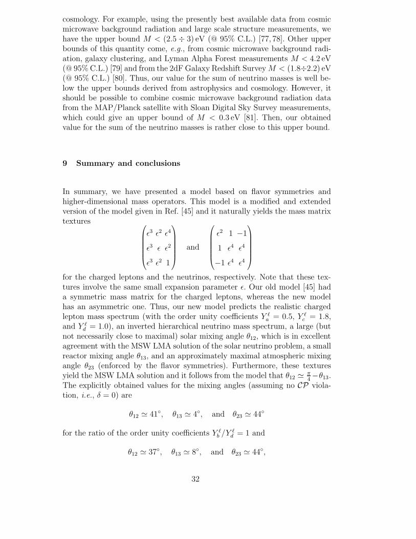
9 Summary and conclusions

In summary, we have presented a model based on flavor symmetries andhigher-dimensional mass operators. This model is a modified and extendedversion of the model given in Ref. [45] and it naturally yields the mass matrixtextures

ε3 ε2 ε4

ε3 ε ε2

ε3 ε2 1

and

ε2 1 −1

1 ε4 ε4

−1 ε4 ε4

for the charged leptons and the neutrinos, respectively. Note that these tex-tures involve the same small expansion parameter ε. Our old model [45] hada symmetric mass matrix for the charged leptons, whereas the new modelhas an asymmetric one. Thus, our new model predicts the realistic chargedlepton mass spectrum (with the order unity coefficients Y `

a = 0.5, Y `c = 1.8,

and Y `d = 1.0), an inverted hierarchical neutrino mass spectrum, a large (but

not necessarily close to maximal) solar mixing angle θ12, which is in excellentagreement with the MSW LMA solution of the solar neutrino problem, a smallreactor mixing angle θ13, and an approximately maximal atmospheric mixingangle θ23 (enforced by the flavor symmetries). Furthermore, these texturesyield the MSW LMA solution and it follows from the model that θ12 ' π

4−θ13.

The explicitly obtained values for the mixing angles (assuming no CP viola-tion, i.e., δ = 0) are

θ12 ' 41◦, θ13 ' 4◦, and θ23 ' 44◦

for the ratio of the order unity coefficients Y `b /Y `

d = 1 and

θ12 ' 37◦, θ13 ' 8◦, and θ23 ' 44◦,

32

for the ratio of the order unity coefficients Y `b /Y `

d = 2. Both these sets of theleptonic mixing angles are in very good agreement with present experimen-tal data. In addition, our values are not in conflict with limits coming fromneutrinoless double β-decay, astrophysics, and cosmology.

Finally, we have also (in the Appendix) presented a scheme for how to trans-form any given 3× 3 unitary matrix to the “standard” parameterization formof the Particle Data Group.

Acknowledgements

We would like to thank Martin Freund, Walter Grimus, Steve King, and HolgerBech Nielsen for useful discussions and comments.

This work was supported by the Swedish Foundation for International Coop-eration in Research and Higher Education (STINT) [T.O.], the Wenner-GrenFoundations [T.O.], the Magnus Bergvall Foundation (Magn. Bergvalls Stif-telse) [T.O.], and the “Sonderforschungsbereich 375 fur Astro-Teilchenphysikder Deutschen Forschungsgemeinschaft” [T.O. and G.S.].

A Transformation of any 3 × 3 unitary matrix to the “standard”parameterization form

The “standard” parameterization form of a 3× 3 unitary matrix according tothe Particle Data Group [24] reads

U =

C2C3 S3C2 S2e−iδ

−S3C1 − S1S2C3eiδ C1C3 − S1S2S3e

iδ S1C2

S1S3 − S2C1C3eiδ −S1C3 − S2S3C1e

iδ C1C2

, (A.1)

where Sa ≡ sin θa, Ca ≡ cos θa (for a = 1, 2, 3), and δ is the physical CPviolation phase. Here θ1 ≡ θ23, θ2 ≡ θ13, and θ3 ≡ θ12 are the Euler (mixing)angles. Note that four of the entries of the matrix U in Eq. (A.1) are real, i.e.,the 1-1, 1-2, 2-3, and 3-3 entries. Furthermore, the matrix U in Eq. (A.1) canbe decomposed as follows:

33

U = O23(θ23)U13(θ13, δ)O12(θ12)

=

1 0 0

0 C23 S23

0 −S23 C23

C13 0 S13e−iδ

0 1 0

−S13eiδ 0 C13

C12 S12 0

−S12 C12 0

0 0 1

, (A.2)

where Cab ≡ cos θab, Sab ≡ sin θab (for a, b = 1, 2, 3), and Oab(θab) is a rotationby an angle θab in the ab-plane. If δ = 0, then U13(θ13, 0) = O13(θ13).

Here we will show how to transform any given 3 × 3 unitary matrix to the“standard” parameterization form. A 3× 3 unitary matrix

U ≡ (Uab) =

U11 U12 U13

U21 U22 U23

U31 U32 U33

(A.3)

where a, b = 1, 2, 3, obeys U †U = UU † = 13 (9 unitarity conditions) and istherefore characterized by 9 real parameters, since a general 3 × 3 complexmatrix is characterized by 18 real parameters (9 complex parameters). Outof these 9 parameters, 3 are Euler (mixing) angles and 6 are phase factors(phases). Not all of the 6 phases enter into expressions for physically measur-able quantities. Only those phases are physical 11 , which cannot be eliminated

11 In the transition probability formulas for neutrino oscillations (να → νβ)

P (να → νβ) ≡ Pαβ ≡ Pαβ(L) =3∑

a=1

3∑b=1

Jabαβei

∆m2ab

2EL,

where α, β = e, µ, τ ; L is the neutrino baseline length, E is the neutrino energy,Jab

αβ ≡ U∗αaUβaUαbU

∗βb are the amplitude parameters, and ∆m2

ab ≡ m2a − m2

b arethe neutrino mass squared differences, we observe that the matrix elements of theleptonic mixing matrix U = (Uαa), where α = e, µ, τ and a = 1, 2, 3, only appear inthe amplitude parameters Jab

αβ . It is obvious from the definitions of the amplitudeparameters

Jabαβ ≡ U∗

αaUβaUαbU∗βb

to see that they are invariant under phase transformations of the following kind

Uαa → U ′αa = eiϕαUαae

−iϕa ,

where ϕα, ϕa ∈ R are arbitrary parameters, i.e., J ′abαβ = Jab

αβ . Thus, the transitionprobability formulas may only depend on phases in the matrix U , which cannot beabsorbed by the above phase transformations (see Eq. (A.4) for the correspondingmatrix form). The number of such phases is equal to 1 (in the 3× 3 case), i.e., theCP violation phase δ [82,83].

34

by the transformation

U → U ′ = Φ`UΦ†ν , (A.4)

where the matrices Φ` ≡ diag (eiϕe, eiϕµ , eiϕτ ) and Φν ≡ diag (eiϕ1 , eiϕ2, eiϕ3)can always be put on the forms

Φ` = eiϕ`Φ`′ , (A.5)

Φν = eiϕνΦν′ (A.6)

such that det Φ`′ = 1 and det Φν′ = 1, where Φ`′ ≡ diag (eiϕe′ , eiϕµ′ , eiϕτ ′ ) andΦν′ ≡ diag (eiϕ1′ , eiϕ2′ , eiϕ3′ ). This means that ϕα = ϕ` + ϕα′ (α = e, µ, τ) andϕa = ϕν + ϕa′ (a = 1, 2, 3), where ϕe′ + ϕµ′ + ϕτ ′ = 0 and ϕ1′ + ϕ2′ + ϕ3′ = 0.Thus, we have

U → U ′ = ei(ϕ`−ϕν)Φ`′UΦν′ = eiϕΦ`′UΦν′ , (A.7)

where ϕ ≡ ϕ` − ϕν , and on matrix form, we find that

U ′ = eiϕ

U11ei(ϕe′−ϕ1′ ) U12e

i(ϕe′−ϕ2′ ) U13ei(ϕe′−ϕ3′ )

U21ei(ϕµ′−ϕ1′ ) U22e

i(ϕµ′−ϕ2′ ) U23ei(ϕµ′−ϕ3′ )

U31ei(ϕτ ′−ϕ1′ ) U32e

i(ϕτ ′−ϕ2′ ) U33ei(ϕτ ′−ϕ3′ )

. (A.8)

Assuming now that the matrix U ′ in Eq. (A.8) is on the “standard” param-eterization form as displayed in Eq. (A.1), we identify from the 1-1, 1-2, 1-3,2-3, and 3-3 entries that

C2C3 =eiϕU11ei(ϕe′−ϕ1′ ) = |U11|ei(arg U11+ϕ+ϕe′−ϕ1′ ), (A.9)

S3C2 =eiϕU12ei(ϕe′−ϕ2′ ) = |U12|ei(arg U12+ϕ+ϕe′−ϕ2′ ), (A.10)

S2e−iδ =eiϕU13e

i(ϕe′−ϕ3′ ) = |U13|ei(arg U13+ϕ+ϕe′−ϕ3′ ), (A.11)

S1C2 =eiϕU23ei(ϕµ′−ϕ3′ ) = |U23|ei(arg U23+ϕ+ϕµ′−ϕ3′ ), (A.12)

C1C2 =eiϕU33ei(ϕτ ′−ϕ3′ ) = |U33|ei(arg U33+ϕ+ϕτ ′−ϕ3′ ). (A.13)

Taking the imaginary parts of Eqs. (A.9), (A.10), (A.12), and (A.13), we arriveat

0 =arg U11 + ϕ + ϕe′ − ϕ1′, (A.14)

0 =arg U12 + ϕ + ϕe′ − ϕ2′, (A.15)

0 =arg U23 + ϕ + ϕµ′ − ϕ3′ , (A.16)

0 =arg U33 + ϕ + ϕτ ′ − ϕ3′ , (A.17)

which together with the two conditions

35

ϕe′ + ϕµ′ + ϕτ ′ = 0, (A.18)

ϕ1′ + ϕ2′ + ϕ3′ = 0 (A.19)

make up a system of equations. Note that the overall phase ϕ can be absorbedinto the arg Uab’s, i.e., arg Uab +ϕ → arg Uab. The system of equations includessix equations and six unknown quantities, i.e., ϕα′ (α = e, µ, τ) and ϕa′ (a =1, 2, 3), and thus, it has a unique solution. This solution is

ϕe′ =1

3(−2 arg U11 − 2 arg U12 − arg U23 − arg U33) , (A.20)

ϕµ′ =1

3(arg U11 + arg U12 − arg U23 + 2 argU33) , (A.21)

ϕτ ′ =−ϕe′ − ϕµ′, (A.22)

ϕ1′ =1

3(arg U11 − 2 argU12 − arg U23 − arg U33) , (A.23)

ϕ2′ =1

3(−2 arg U11 + arg U12 − arg U23 − arg U33) , (A.24)

ϕ3′ =−ϕ1′ − ϕ2′ . (A.25)

Inserting the solution into Eqs. (A.9) - (A.13), we obtain

C2C3 = |U11|, (A.26)

S3C2 = |U12|, (A.27)

S2e−iδ = |U13|ei(arg U13−arg U11−arg U12−arg U23−arg U33), (A.28)

S1C2 = |U23|, (A.29)

C1C2 = |U33|. (A.30)

Thus, it follows from Eq. (A.28) by taking the real and imaginary parts,respectively, that

S2 = |U13| ⇒ θ13 ≡ θ2 = arcsin S2 = arcsin |U13|, (A.31)

−δ =− arg U11 − arg U12 + arg U13 − arg U23 − arg U33. (A.32)

Dividing Eq. (A.27) by Eq. (A.26), we find that

S3

C3

=∣∣∣∣U12

U11

∣∣∣∣ ⇒ θ12 ≡ θ3 = arctanS3

C3

= arctan∣∣∣∣U12

U11

∣∣∣∣ , (A.33)

and similarly, dividing Eq. (A.29) by Eq. (A.30), we find that

S1

C1

=∣∣∣∣U23

U33

∣∣∣∣ ⇒ θ23 ≡ θ1 = arctanS1

C1

= arctan∣∣∣∣U23

U33

∣∣∣∣ . (A.34)

In summary, the parameters of the “standard” parameterization form is givenas

36

θ12 =arctan∣∣∣∣U12

U11

∣∣∣∣ , (A.35)

θ13 =arcsin |U13|, (A.36)

θ23 =arctan∣∣∣∣U23

U33

∣∣∣∣ , (A.37)

δ =arg U11 + arg U12 − arg U13 + arg U23 + arg U33 (A.38)

in terms of the entries of any 3 × 3 unitary matrix U = (Uab). Note thatthese parameters are uniquely determined by the entries in the first row andthird column (U11, U12, U13, U23, and U33) only as well as the overall phaseϕ. The other entries are completely restricted by and follow directly from theunitarity conditions (U †U = UU † = 13).

References

[1] N. Cabibbo, Phys. Rev. Lett. 10 (1963) 531.

[2] M. Kobayashi and T. Maskawa, Prog. Theor. Phys. 49 (1973) 652.

[3] R. Dermisek and S. Raby, Phys. Rev. D 62 (2000) 015007, hep-ph/9911275.

[4] S.F. King and G.G. Ross, Phys. Lett. B 520 (2001) 243, hep-ph/0108112.

[5] Super-Kamiokande Collaboration, Y. Fukuda et al., Phys. Rev. Lett. 81 (1998)1562, hep-ex/9807003.

[6] Super-Kamiokande Collaboration, Y. Fukuda et al., Phys. Rev. Lett. 82 (1999)2644, hep-ex/9812014.

[7] Super-Kamiokande Collaboration, S. Fukuda et al., Phys. Rev. Lett. 85 (2000)3999, hep-ex/0009001.

[8] Super-Kamiokande Collaboration, T. Toshito, hep-ex/0105023.

[9] M. Shiozawa, talk given at the XXth International Conference on NeutrinoPhysics & Astrophysics (Neutrino 2002), Munich, Germany, 2002.

[10] Super-Kamiokande Collaboration, S. Fukuda et al., Phys. Rev. Lett. 86 (2001)5651, hep-ex/0103032.

[11] Super-Kamiokande Collaboration, M.B. Smy, hep-ex/0106064.

[12] Super-Kamiokande Collaboration, S. Fukuda et al., hep-ex/0205075.

[13] M. Smy, talk given at the XXth International Conference on Neutrino Physics& Astrophysics (Neutrino 2002), Munich, Germany, 2002.

[14] SNO Collaboration, Q.R. Ahmad et al., Phys. Rev. Lett. 87 (2001) 071301,nucl-ex/0106015.

37

[15] SNO Collaboration, Q.R. Ahmad et al., nucl-ex/0204008.

[16] SNO Collaboration, Q.R. Ahmad et al., Phys. Rev. Lett. (to be published),nucl-ex/0204009.

[17] A. Hallin, talk given at the XXth International Conference on Neutrino Physics& Astrophysics (Neutrino 2002), Munich, Germany, 2002.

[18] S.P. Mikheyev and A.Y. Smirnov, Yad. Fiz. 42 (1985) 1441, [Sov. J. Nucl. Phys.42 (1985) 913].

[19] S.P. Mikheyev and A.Y. Smirnov, Nuovo Cimento C 9 (1986) 17.

[20] L. Wolfenstein, Phys. Rev. D 17 (1978) 2369.

[21] J.N. Bahcall, M.C. Gonzalez-Garcia and C. Pena-Garay, J. High Energy Phys.08 (2001) 014, hep-ph/0106258.

[22] J.N. Bahcall, M.C. Gonzalez-Garcia and C. Pena-Garay, J. High Energy Phys.04 (2002) 007, hep-ph/0111150.

[23] J.N. Bahcall, M.C. Gonzalez-Garcia and C. Pena-Garay, hep-ph/0204314.

[24] Particle Data Group, D.E. Groom et al., Eur. Phys. J. C 15 (2000) 1,http://pdg.lbl.gov/.

[25] L.E. Ibanez and G.G. Ross, Phys. Lett. B 332 (1994) 100, hep-ph/9403338.

[26] P. Binetruy and P. Ramond, Phys. Lett. B 350 (1995) 49, hep-ph/9412385.

[27] Q. Shafi and Z. Tavartkiladze, Phys. Lett. B 482 (2000) 145, hep-ph/0002150.

[28] R.N. Mohapatra and S. Nussinov, Phys. Rev. D 60 (1999) 013002,hep-ph/9809415.

[29] C. Wetterich, Phys. Lett. B 451 (1999) 397, hep-ph/9812426.

[30] W. Grimus and L. Lavoura, J. High Energy Phys. 07 (2001) 045,hep-ph/0105212.

[31] R.N. Mohapatra, A. Perez-Lorenzana and C.A. de Sousa Pires, Phys. Lett. B474 (2000) 355, hep-ph/9911395.

[32] H. Fritzsch and Z.z. Xing, Phys. Lett. B 372 (1996) 265, hep-ph/9509389.

[33] H. Fritzsch and Z.z. Xing, Phys. Lett. B 440 (1998) 313, hep-ph/9808272.

[34] H. Fritzsch and Z.z. Xing, Prog. Part. Nucl. Phys. 45 (2000) 1, hep-ph/9912358.

[35] M. Fukugita, M. Tanimoto and T. Yanagida, Phys. Rev. D 57 (1998) 4429,hep-ph/9709388.

[36] M. Fukugita, M. Tanimoto and T. Yanagida, Phys. Rev. D 59 (1999) 113016,hep-ph/9809554.

[37] M. Tanimoto, Phys. Rev. D 59 (1999) 017304, hep-ph/9807283.

38

[38] S.K. Kang and C.S. Kim, Phys. Rev. D 59 (1999) 091302, hep-ph/9811379.

[39] M. Tanimoto, T. Watari and T. Yanagida, Phys. Lett. B 461 (1999) 345,hep-ph/9904338.

[40] I. Dorsner and S.M. Barr, Nucl. Phys. B 617 (2001) 493, hep-ph/0108168.

[41] S. King, talk given at the XXth International Conference on Neutrino Physics& Astrophysics (Neutrino 2002), Munich, Germany, 2002.

[42] H.J. He, D.A. Dicus and J.N. Ng, Phys. Lett. B 536 (2002) 83, hep-ph/0203237.

[43] M. Lindner and W. Winter, hep-ph/0111263.

[44] S.F. King, hep-ph/0204360.

[45] T. Ohlsson and G. Seidl, Phys. Lett. B 537 (2002) 95, hep-ph/0203117.

[46] V. Barger et al., Phys. Lett. B 437 (1998) 107, hep-ph/9806387.

[47] S. Weinberg, Phys. Rev. Lett. 43 (1979) 1566.

[48] F. Wilczek and A. Zee, Phys. Rev. Lett. 43 (1979) 1571.

[49] C.D. Froggatt and H.B. Nielsen, Nucl. Phys. B 147 (1979) 277.

[50] K.S. Babu and C.N. Leung, Nucl. Phys. B 619 (2001) 667, hep-ph/0106054.

[51] C.D. Froggatt, H.B. Nielsen and Y. Takanishi, Nucl. Phys. B (to be published),hep-ph/0201152.

[52] H.B. Nielsen and Y. Takanishi, hep-ph/0205180.

[53] M. Gell-Mann, P. Ramond and R. Slansky, Complex Spinors and UnifiedTheories, in Supergravity, Proceedings of the Workshop on Supergravity, StonyBrook, New York, 1979, edited by P. van Nieuwenhuizen and D.Z. Freedman(North-Holland, Amsterdam, 1979), p. 315.

[54] T. Yanagida, in Proceedings of the Workshop on the Unified Theory andBaryon Number in the Universe, edited by O. Sawada and A. Sugamoto (KEK,Tsukuba, 1979), p. 79.

[55] R.N. Mohapatra and G. Senjanovic, Phys. Rev. Lett. 44 (1980) 912.

[56] M. Leurer, Y. Nir and N. Seiberg, Nucl. Phys. B 398 (1993) 319,hep-ph/9212278.

[57] A. Perez-Lorenzana and C.A. de Sousa Pires, Phys. Lett. B 522 (2001) 297,hep-ph/0108158.

[58] L.M. Krauss and F. Wilczek, Phys. Rev. Lett. 62 (1989) 1221.

[59] L.E. Ibanez and G.G. Ross, Phys. Lett. B 260 (1991) 291.

[60] E. Witten, hep-ph/0201018.

39

[61] M. Sher, Phys. Rept. 179 (1989) 273.

[62] E. Witten, Phys. Lett. B 105 (1981) 267.

[63] M. Leurer, Y. Nir and N. Seiberg, Nucl. Phys. B 420 (1994) 468,hep-ph/9310320.

[64] T. Ohlsson and H. Snellman, J. Math. Phys. 41 (2000) 2768, hep-ph/9910546,42 (2001) 2345(E).

[65] T. Ohlsson, Phys. Scripta T93 (2001) 18.

[66] Z. Maki, M. Nakagawa and S. Sakata, Prog. Theor. Phys. 28 (1962) 870.

[67] CHOOZ Collaboration, M. Apollonio et al., Phys. Lett. B 420 (1998) 397,hep-ex/9711002.

[68] CHOOZ Collaboration, M. Apollonio et al., Phys. Lett. B 466 (1999) 415,hep-ex/9907037.

[69] CHOOZ Collaboration, C. Bemporad, Nucl. Phys. B (Proc. Suppl.) 77 (1999)159.

[70] S.M. Bilenky and S.T. Petcov, Rev. Mod. Phys. 59 (1987) 671, 61 (1989)169(E).

[71] S.M. Bilenky, S. Pascoli and S.T. Petcov, Phys. Rev. D 64 (2001) 053010,hep-ph/0102265.

[72] M. Lindner, T. Ohlsson and G. Seidl, Phys. Rev. D 65 (2002) 053014,hep-ph/0109264.

[73] S. Pascoli and S.T. Petcov, (2002), hep-ph/0205022.

[74] H.V. Klapdor-Kleingrothaus, Nucl. Phys. B (Proc. Suppl.) 100 (2001) 309,hep-ph/0102276.

[75] IGEX Collaboration, C.E. Aalseth et al., Phys. Atom. Nucl. 63 (2000) 1225,[Yad. Fiz. 63 (2000) 1299].

[76] IGEX Collaboration, C.E. Aalseth et al., Phys. Rev. D 65 (2002) 092007,hep-ex/0202026.

[77] S. Hannestad, astro-ph/0205223.

[78] S. Hannestad, talk given at the XXth International Conference on NeutrinoPhysics & Astrophysics (Neutrino 2002), Munich, Germany, 2002.

[79] X. Wang, M. Tegmark and M. Zaldarriaga, Phys. Rev. D 65 (2002) 123001,astro-ph/0105091.

[80] Ø. Elgarøy et al., astro-ph/0204152.

[81] W. Hu, D.J. Eisenstein and M. Tegmark, Phys. Rev. Lett. 80 (1998) 5255,astro-ph/9712057.

[82] S.M. Bilenky, J. Hosek and S.T. Petcov, Phys. Lett. B 94 (1980) 495.

[83] M. Doi et al., Phys. Lett. B 102 (1981) 323.

40