Sea Grant College Program Massachusetts Institute of Technology Cambridge, Massachusetts 02139 NOAA Grant No. NA10OAR4170086 Project No. 2006-R/RT-2/RCM-17 Reprinted from the Journal of Microelectromechanical Systems, Vol. 21, Pages 897-907, August 2012.

A FLEXIBLE UNDERWATER PRESSURE SENSOR ARRAY USING A CONDUCTIVE ELASTOMER

STRAIN GAUGE

F. M. Yaul, V. Bulovic and J. H. Lang

MITSG 12-11

JOURNAL OF MICROELECTROMECHANICAL SYSTEMS 1

A Flexible Underwater Pressure Sensor Arrayusing a Conductive Elastomer Strain Gauge

Frank M. Yaul, Member, IEEE, Vladimir Bulovic, and Jeffrey H. Lang, Fellow, IEEE

Abstract—This paper presents a flexible pressure sensor ar-ray which is demonstrated to transduce underwater pressurevariations produced by moving objects and surface waves. Thesensors exhibit a 0.0014 fractional resistance change per 100pascals, achieving a pressure resolution of 1.5 pascals using a 16-bit analog/digital converter. Additionally, sensor operation whilebent to a 0.5 m radius of curvature is demonstrated. Each sensorconsists of a strain-concentrating polydimethylsiloxane (PDMS)diaphragm and a resistive strain gauge made of a conductivecarbon black-PDMS composite. A one-dimensional array of 4sensors with a 15 mm center-to-center spacing is fabricated,and the dynamic response of the sensors is characterized andmodeled.

Index Terms—Pressure sensor arrays, sensor design, character-ization, modeling, strain gauge, fabrication, flexible, conductiveelastomers, PDMS, carbon black

I. INTRODUCTION

CURRENT technologies used by autonomous underwatervehicles (AUVs) for remote detection of underwater

objects include sonar and vision-based systems [1]. However,sonar suffers from multipath propogation issues in the clutteredseabed environment, and vision-based systems are limited bythe turbidity of the sea water. Additionally, both systems areforms of active sensing and must emit energy in the formof acoustic waves or light in order to operate. Thus, they areinherently less energy-efficient and less covert when comparedto passive detection systems which only measure ambientsignals in the environment and do not emit energy. In lightof these issues, there has been recent interest in a biomimeticapproach to underwater sensing involving using sensor arraysto create an artificial version of a fish’s lateral line. The lateralline is an organ possessed by all fish which contains an arrayof flow sensors that transduce pressure variations in the water[2]. Many complex behaviors of fish may be attributed to thelateral line, including navigation in cluttered environments inthe absence of light [3], tracking prey by their wake [4], anddiscriminating the size, velocity, and shape of nearby objects[5]. Giving such functionality to AUVs is a current topic ofresearch [6], and is the motivation for this work.

Attempts to construct a pressure sensor array using individ-ual off-the-shelf silicon MEMS pressure sensors are limited

The work of F. M. Yaul was supported by the MIT Sea Grant R/RT-2/RC-17with Dr. M. S. Triantafyllou as program manager, and by the National ScienceFoundation through the Center for Energy Efficient Electronics Science (E3S).This work was presented in part at the 25th International Conference on MicroElectro Mechanical Systems, Paris, France, January 29-February 2, 2012.

F. M. Yaul, V. Bulovic, and J. H. Lang are with the Department of ElectricalEngineering and Computer Science, Massachusetts Institute of Technology,Cambridge, MA, 02139 USA (e-mail: frank y@mit.edu)

in their spatial resolution [7]. While it is possible to increasethe spatial resolution by fabricating a pressure sensor arrayon a single silicon substrate, the silicon does not exhibitthe flexibility or chemical robustness required for use as anartificial lateral line. Silicon MEMS flow sensor arrays havealso been used to create artificial lateral lines, though they tooare fragile and lack flexibility due to the silicon substrate andmust be protected from the water with a parylene coating [6].

This work, based on [8] and [9], addresses these issuesby constructing the pressure sensor array entirely from anelastomer material set, allowing the array to be waterproofand flexible. The sensors are modeled after silicon MEMSpressure sensors [10] which use a strain-concentrating di-aphragm with a resistive strain gauge. Adopting a MEMS-based design allows the spatial resolution to be increasedthrough device miniaturization using planar batch fabricationtechniques. In this device, polydimethylsiloxane (PDMS) isused for the substrate and the diaphragm, while a conductiveelastomer composite made of PDMS doped with carbon blacknanoparticles is used as the resistive strain gauge material. Thecarbon black-PDMS composite is used since it is chemicallyand mechanically compatible with the PDMS substrate. Thepressure sensor array consists of individual sensors arranged ina one-dimensional strip. The array’s flexibility allows it to beexternally mounted along the curved hull of an AUV where itcan transduce tiny underwater pressure variations on the orderof 10 pascals produced by relative motion between objectsand the water surrounding the vehicle. Thus, the informationabout the fluid flow provided by the array enables the passivedetection of underwater obstructions or targets [7], and canalso be used to enhance the AUV’s propulsive efficiency andmaneuverability [11].

Prior work in the area of polymer and elastomer-basedpressure sensor arrays is geared towards tactile sensing ap-plications where objects physically contact the sensor andgenerate large pressure signals in the tens to hundreds of kilo-pascals. Many of these works provide a static characterizationof the sensor by taking discrete data points spaced tens tohundreds of kilopascals apart [12]–[15]. Unfortunately, thesepolymer and elastomer-based pressure sensors have typicallybeen unable to achieve high pressure resolution due to thehysteresis inherent in the viscoelastic behavior of polymermaterials [16]. One elastomer-based pressure sensor intendedto have a high pressure sensitivity uses a composite materialmade of carbon nanotubes and PDMS [17]. However, it alsoprovides only a static characterization of the sensor, and thereis no discussion on hysteresis inherent in the viscoelastic

0000–0000/00$00.00 c© 2000 IEEE

JOURNAL OF MICROELECTROMECHANICAL SYSTEMS 2

(b)

(c)

Air cavity PDMS

Rigid backing

2 mm

1 mm-thick diaphragm 100 µm-thick

strain

gauge

(a)

Isrc

+ V1 -

+ V2 -

+ V3 -

+ V4 -

Diaphragm 1 mm

Channel Strain

gauge PDMS Substrate

10 mm 2 mm

5 mm

Fig. 1. Diagrams and photograph of the pressure sensor array showing (a)top view, (b) side view, and (c) photograph.

behavior of the elastomers.This paper provides a more thorough sensor characterization

by testing the dynamic response, and presents a quantitativemodel that accounts for the viscoelasticity of the PDMSand the nonlinear resistance-strain relationship of the carbonblack-PDMS composite. Overall, this MEMS-based elastomerpressure sensor array departs significantly from prior polymerand elastomer-based pressure sensors in that it is intended notfor tactile applications, but for use as an artificial lateral linewhich requires high pressure sensitivity, flexibility, and a wa-terproof structure. Additionally, this paper describes a Kelvinprobe strain gauge structure which enables the conductiveelastomer strain gauge to contact rigid metal wires off of thePDMS diaphragm without losing pressure sensitivity due tothe additional series resistance created by the lengthened straingauge contacts. Finally, underwater operation is demonstrated.

II. PRESSURE SENSOR ARRAY DESIGN

The pressure sensor array in this work consists of 4 pressuresensing cells as depicted in Figure 1. Each cell in the arraycomprises 4 main components which are detailed in thefollowing sections. The PDMS substrate gives the array itsflexibility and waterproofing. A strain-concentrating squarePDMS diaphragm covers the pressure sensor’s internal cavity.The diaphragm deflects in response to a pressure differencebetween the internal cavity and the environment. The resistivestrain gauge made of the carbon black-PDMS composite ispatterned onto the underside of the diaphragm so that itis shielded from the water. Lastly, a pressure equilibrationchannel connects the cavities of all 4 pressure sensing cells

to an external pressure reference which allows the array tooperate at arbitrary water depth.

A. PDMS Substrate

PDMS is selected as the flexible substrate and structuralmaterial for the pressure sensor array because it has beenwidely used in MEMS and is known to provide electricalinsulation and waterproofing [18]. Additionally, many well-developed PDMS micropatterning techniques exist [19]. Tocharacterize the its viscoelastic behavior, a PDMS cantilever isconstructed and mechanically tested. The PDMS’s stress-strainresponse, known as the tensile modulus E, is proportionalto the PDMS cantilever’s force-displacement relationship asshown by

K =F

x=EWH3

4L3(1)

where K is the cantilever spring constant [10], F is the forceapplied to the cantilever’s free end, x is the displacement ofthe free end, the width W is 2 cm, the thickness H is 0.5 cm,the length L is 3 cm. For small strains, E may be modeledwith the Burger model for viscoelasticity [16], shown in Figure2(a). The Burger model consists of a system of springs anddashpots that may be represented with an s-domain transferfunction as

E(s) =ε

σ(s) =

1

kP + scP+

1

kS− 1

scS(2)

where kS , cS , kP , and cP are the model parameters. Todetermine these parameters, a square wave of displacementx is applied to the free end of a PDMS cantilever and theforce F is measured. The model parameters given in Figure2(a) are fit to the data shown in Figure 2(b). A bode plot isgenerated from the model, shown in Figure 2(c).

The corner frequency ωS denoted in the bode plot corre-sponds to the time constant τS of the relaxation of the seriesdashpot cS . Since kP >> kS , both kP and cP may be ignoredand τS may be approximated as

τS = cS/kS = 111 s (3)

which is the time constant of the series system comprising thedashpot cS and spring kS . Stress waveforms slower than ωS

cause significant displacement of cS . This behavior is knownas viscoelastic creep and is responsible for the elastomer’smechanical hysteresis. Above ωS , the mechanical responsemay be approximated solely by kS as shown in the bode plot,such that E = kS = 2.35 MPa, which is close to the valueof E = 1.7 MPa presented in [18]. Consequently, the PDMSdiaphragms of the pressure sensor array will have a linearstress-strain response to dynamic (AC) signals, though thestatic (DC) response will exhibit hysteresis due to viscoelasticcreep.

B. Strain-Concentrating PDMS Diaphragm

A strain-concentrating square PDMS diaphragm transducesa pressure difference between the environment and the sensor’sinternal cavity into a strain. Because of this, the dimensionsof the diaphragm, given in Figure 1, are the main mechanical

JOURNAL OF MICROELECTROMECHANICAL SYSTEMS 3

kS

kP

cS

cP

ε

σ

(a)

0

2

4

Dis

pla

cem

ent

(mm

)

0 10 20 30 40

0

0.1

0.2

Forc

e (N

)

Time (s)

Measured Data Simulation

(b)

-120

-100

-80

Magnit

ude

(dB

)

10-4 10-2 100 102 -45

0

45

90

Ph

ase

(d

eg)

Frequency (rad/s)

ωS

1 / kS

(c)

kS=2.35 Mpa

cS=259 MPa·s

kP=15.1 MPa

cP=8.64 MPa·s

Fig. 2. (a) Burger model for viscoelasticity. (b) Dynamic response of PDMScantilever showing applied displacement (top) and measured force comparedto the simulated force (bottom). Due to the good curve fit, the two are difficultto distinguish. (c) Bode plot of ε/σ.

parameters that influence the pressure sensitivity of the device.For deflections less than the thickness of the diaphragm,the load-deflection behavior of a square diaphragm may beapproximated by

P =π4EH3

6(1 − ν2)L4· c (4)

where P is the pressure difference across the diaphragm, cis the deflection at the center of the diaphragm, H is thediaphragm thickness, and L is the side length of the squarediaphragm [10]. The Poisson’s ratio ν may be approximated as0.5 for PDMS since it is an elastomer. The tensile modulus Eis taken to be 2.35 MPa as determined in Section II-A. UsingEquation 4, the diaphragm dimensions may be chosen to keepthe deflection much smaller than the membrane thickness forpressures up to the maximum pressure of interest. Based on theunderwater pressure waveforms produced by moving objectsin [7], 1 kPa is a generous upper pressure bound.

Since the focus of this work is not miniaturization, conser-vative dimensions are chosen for the sensor array. With L = 10mm and H = 1 mm, aluminum molds are machined to createthe cavity and membrane structure. For those dimensions,Equation 4 predicts a 0.2 mm deflection in response toa 1 kPa pressure. This deflection is smaller than H , thusachieving a self-consistent result. Though the depth of thecavity only needs to be large enough to accomodate thisdeflection, the depth is chosen to be 2 mm to provide a largepressure reservoir. This way, the volume change of the cavitydue to diaphragm deflection is insignificant, preventing aircompression from reducing sensitivity. The diaphragm center-to-center spacing sets the spatial resolution of the sensor. Thespacing is chosen to be 15 mm which provides a 5 mm

gap between the edges of adjacent diaphragms and preventsmechanical crosstalk. In comparison, sensor spacings on theorder of 50 mm are used in the object identification and vortextracking experiments performed in [7].

This diaphragm will have a first resonance frequency f0based on its mass and spring constant, which may be estimatedusing the Rayleigh-Ritz method [20]. This gives

f0 = 1.654 · CHL2

(5)

where C is the speed of sound in the diaphragm material, H isthe diaphragm thickness, and L is the diaphragm side length.C is related to the material parameters by

C2 =E

ρ(1 − ν2)(6)

where E is the tensile modulus, ρ is the density of the PDMS,and ν is the poisson’s ratio. Evaluating Equation 5 yieldsf0 = 940 Hz. This number sets an upper bound on thebandwidth of the sensor. Realistically, viscous damping due tothe water, air, and PDMS itself lower the sensor bandwidth. Abandwidth limit due to the carbon black-PDMS strain gauge’sstrain-resistance response would also be a possibility, thoughthis does not appear to be the case based on results from thesensor characterization experiments of Section IV.

Lastly, the sensor may be mounted on a curved surface aslong as the strain on the diaphragms induced by the curvatureεbend does not exceed the maximum strain experienced bythe diaphragms in the small-deflection regime εmax. Thismaximum strain εmax is given in [10] as

εmax =6

π2(1 − ν2)(

L

H)2P

E= 0.02 (7)

where P is the maximum differential pressure allowed acrossthe diaphragm while keeping it well in the small-deflectionregime, and is determined to be 1 kPa in Section II-B. εbendshould be kept much smaller than εmax so that it does notsignificantly affect the deflection of the diaphragm. εbend maybe estimated as

εbend = z/R (8)

where R is the radius of curvature, and z is the radial distancefrom neutral axis to the plane of the array containing thediaphragms. The thickness of the sensor array is 4 mm, sothe neutral axis is approximately at 2 mm, making z ≈ 2 mm.For R = 0.5 m, εbend = 0.2εmax so the array’s diaphragmwill still operate in the linear regime at this curvature.

C. Pressure Equilibration Channel

As shown in Figure 1, the pressure equilibration channelconnects all 4 cavities to an external port. A syringe maybe connected to this port, enabling dynamic control overthe cavity pressure. During characterization experiments, thisenables actuation of the diaphragms by changing the cavitypressure, as shown in Figure 3(a). For underwater use, atube runs from the channel out into the water. The tubefunctions as a low-pass filter, so that the cavity pressure isset to the DC water pressure. This cancels the large DCpressure that would otherwise damage the sensors, while still

JOURNAL OF MICROELECTROMECHANICAL SYSTEMS 4

1 mL syringe

Pressure sensor array

Tubing

(a)

(b) Tubing Open

to water

Water surface

Δh

Fig. 3. Diagram of pressure equilibration schemes showing (a) syringe setupfor characterization and (b) tube setup for underwater use.

allowing measurement of small-amplitude pressure signals inthe frequencies of interest. Additionally, because all of thecavities share the same pressure, the array is still capableof transducing DC differential pressures between individualsensors, in contrast to underwater microphones which areincapable of transducing any DC pressure.

The difference in depth ∆h of the end of the tube connectedto the water and the depth of the diaphragms determines thepressure bias Pbias applied to the sensor cells, as shown inFigure 3(b). Pbias may be calculated using

Pbias = ρg∆h (9)

where ρ is the density of water and g is Earth’s gravitationalacceleration. The tube method allows for the DC differentialpressure bias across the diaphragms to stay constant, indepen-dent of the depth of the sensors in the water.

D. Carbon Black-PDMS Resistive Strain Gauge

The strain gauge material is chosen to be a composite madeof an elastomer doped with conductive filler particles becauseit satisfies the requirements for conductivity, and chemicaland mechanical compatibility with the PDMS. Several po-tential elastomer-conductive filler composite materials havebeen explored in the literature, including a nickel-siliconecomposite [21], and a carbon black-PDMS composite [22].While both composites vary considerably in their electrical andmechanical characteristics, their syntheses involve the sameprocess of uniformly dispersing the conductive filler particleswithin the elastomer’s matrix, and then fixing them in placeby curing the elastomer. The carbon black-PDMS compositeis chosen due to its smooth strain-resistance relation, as willbe demonstrated by the sensor characterization in Section IV.

The most straightforward method to use the compositematerial as a strain gauge would be to pattern a strip of thecomposite material onto the structure of interest, and connecttwo wires to it using conductive epoxy, creating a 2-point-probe. The center-edge of the diaphragm is the region thatexperiences the greatest strain during deflection [10] so itis an ideal location for the strain guage. Unfortunately, acontact resistance Rcontact exists between the metal contactand the strain gauge resistor of interest Rgauge. Additionally,metal wiring is stiff and cannot be routed onto the PDMSdiaphragm, so the conductive elastomer must be routed offof the diaphragm. This creates an additional series resistanceRtap which reduces sensitivity.

Straining

region

Rigid

base

Wires

Rcontact

Rtap

Itest Vtest +

- Itest

PDMS Diaphragm

Rgauge

Fig. 4. Diagram of the strain gauge on the edge of the PDMS diaphragmillustrating the Kelvin probe geometry.

The 4-point-probe, alternatively known as a Kelvin struc-ture, is shown in Figure 4. This structure solves the contactresistance problem because it allows for measurement ofRgauge alone, without being affected by series resistancesRcontact or Rtap. A constant current Itest is passed throughthe two current terminals while the voltage Vtest is measuredacross the two voltage terminals. Since no current passesthrough the voltage terminals, no voltage appears across theRcontact and Rtap on the voltage terminal branches, meaningthat Vtest is purely the voltage across the resistor Rgauge.As shown in Figure 1, The pressure sensor array uses acomposite structure where the 4 strain gauges share a common2 mm-wide current branch that runs along the length of thearray and is aligned with the edge of the diaphragms. Pairsof voltage taps are placed in each sensor cell to measurethe resistance change at the center of the diaphragm’s edge.The strain gauges are patterned onto the underside of thePDMS diaphragm to prevent them from being shorted whenunderwater.

III. FABRICATION

Figure 5 diagrams the fabrication process. PDMS is castin machined aluminum molds to form the 2 mm-thick cavityand channel structure, and two 1 mm-thick sheets. One of thesheets forms the diaphragms above the cavities, and the otherforms the backplanes below the cavities.

The carbon black-PDMS composite is synthesized by pour-ing uncured Sylgard 184 PDMS and Cabot XC-72 carbonblack powder into a cup in a ratio of 1:6 carbon black:PDMSby mass. This ratio provides a sheet resistance in the kilohmsand gives the mixture with a pasty consistency so that it retainsits shape during the patterning process. Because the powderis very light, it is measured by volume, given its density of 1gram per 15 milliliters. A Kurabo Mazerustar planetary mixingmachine uniformly disperses the conductive filler.

A screen patterning technique is used to pattern the straingauges on the PDMS sheet that will form the diaphragms.The screen is made from an overhead transparency 100 µm inthickness. A milling machine removes material from the screenin the shape of the desired pattern. The screen is placed on topof the PDMS substrate, and the carbon black-PDMS paste isspread over the screen. A glass slide is swept across the screen,removing the excess material. After the screen is removed, a100 µm thick layer of the carbon black-PDMS paste is left

JOURNAL OF MICROELECTROMECHANICAL SYSTEMS 5

1. Pattern strain

gauges

2. Bond wires

3. Bond cavity

4. Bond back

plane

5. Seal

Fig. 5. Process flow for the pressure sensor array.

in the shape of the desired pattern. The entire device is flashcured on a hotplate at 120 oC for 10 minutes while the fillerparticles are still uniformly dispersed. Otherwise, gravity andVan der Waals forces would cause the mixture to dehomoge-nize. While the patterns used in this device have features onthe millimeter scale, further miniaturization is possible withthe screen printing technique. A laser-cut screen is used in[17] to pattern a CNT-PDMS conductive elastomer compositewith 50 µm-scale features. 40-gauge (80 µm) copper magnetwires are bonded to the current and voltage terminals of thestrain gauges using uncured carbon black-PDMS paste as aconductive epoxy. The paste is cured to fix the wires in place.

A thin ∼100 µm layer of uncured PDMS is spread onto thecavity/channel structure. This structure is pressed against thePDMS sheet containing the strain gauges. The bond betweenthe layers is completed by baking the device on a hot plate at120 oC for 10 minutes. The exposed side of the cavity/channelstructure is bonded to the remaining 1 mm-thick PDMS sheetin the same way. Finally, additional PDMS is used to seal theremaining exposed regions of the strain gauges and wires.

IV. CHARACTERIZATION

The completed pressure sensor array is dynamically charac-terized by applying small-amplitude pressure signals at severalDC bias pressures up to 1 kilopascal. This mimics the condi-tions that the sensor is expected to experience when used as anartificial lateral line. The sensor output voltages, proportionalto the strain gauge resistances Rgauge, are recorded. Qualita-tive features of the sensor response are discussed in contextof the underlying mechanism for the carbon black-PDMScomposite’s resistance change, leading to the development ofa quantitative model.

The measurement circuit contains a current source whichfeeds Isrc = 19 µA through the IA and IB terminals of thearray, as shown in Figure 1. Each pair of voltage terminalsV1 through V4 is connected to the differential input of anAD620 instrumentation amplifier which provides a gain of

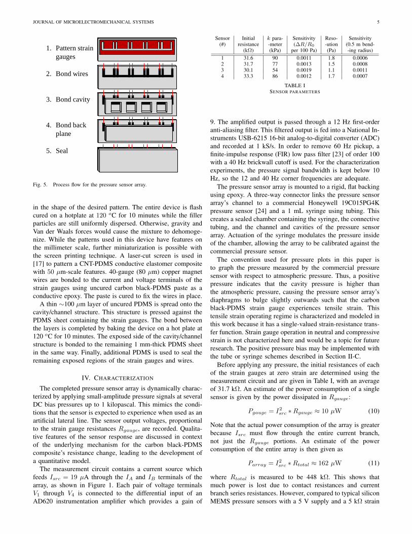
Sensor Initial k para- Sensitivity Reso- Sensitivity(#) resistance -meter (∆R/R0 -ution (0.5 m bend-

(kΩ) (kPa) per 100 Pa) (Pa) -ing radius)1 31.6 90 0.0011 1.8 0.00062 31.7 77 0.0013 1.5 0.00083 30.1 54 0.0019 1.1 0.00114 33.3 86 0.0012 1.7 0.0007

TABLE ISENSOR PARAMETERS

9. The amplified output is passed through a 12 Hz first-orderanti-aliasing filter. This filtered output is fed into a National In-struments USB-6215 16-bit analog-to-digital converter (ADC)and recorded at 1 kS/s. In order to remove 60 Hz pickup, afinite-impulse response (FIR) low pass filter [23] of order 100with a 40 Hz brickwall cutoff is used. For the characterizationexperiments, the pressure signal bandwidth is kept below 10Hz, so the 12 and 40 Hz corner frequencies are adequate.

The pressure sensor array is mounted to a rigid, flat backingusing epoxy. A three-way connector links the pressure sensorarray’s channel to a commercial Honeywell 19C015PG4Kpressure sensor [24] and a 1 mL syringe using tubing. Thiscreates a sealed chamber containing the syringe, the connectivetubing, and the channel and cavities of the pressure sensorarray. Actuation of the syringe modulates the pressure insideof the chamber, allowing the array to be calibrated against thecommercial pressure sensor.

The convention used for pressure plots in this paper isto graph the pressure measured by the commercial pressuresensor with respect to atmospheric pressure. Thus, a positivepressure indicates that the cavity pressure is higher thanthe atmospheric pressure, causing the pressure sensor array’sdiaphragms to bulge slightly outwards such that the carbonblack-PDMS strain gauge experiences tensile strain. Thistensile strain operating regime is characterized and modeled inthis work because it has a single-valued strain-resistance trans-fer function. Strain gauge operation in neutral and compressivestrain is not characterized here and would be a topic for futureresearch. The positive pressure bias may be implemented withthe tube or syringe schemes described in Section II-C.

Before applying any pressure, the initial resistances of eachof the strain gauges at zero strain are determined using themeasurement circuit and are given in Table I, with an averageof 31.7 kΩ. An estimate of the power consumption of a singlesensor is given by the power dissipated in Rgauge:

Pgauge = I2src ∗Rgauge ≈ 10 µW (10)

Note that the actual power consumption of the array is greaterbecause Isrc must flow through the entire current branch,not just the Rgauge portions. An estimate of the powerconsumption of the entire array is then given as

Parray = I2src ∗Rtotal ≈ 162 µW (11)

where Rtotal is measured to be 448 kΩ. This shows thatmuch power is lost due to contact resistances and currentbranch series resistances. However, compared to typical siliconMEMS pressure sensors with a 5 V supply and a 5 kΩ strain

JOURNAL OF MICROELECTROMECHANICAL SYSTEMS 6

1 1.005 1.01 1.015 1.02 0

200

400

600

800

1000

Pre

ssu

re (

Pa

)

R / R0

(a)

(b)

0

500

1000 P

ress

ure

(P

a)

0 20 40 60 80 100 1

1.01

1.02

1.03

1.04

Time (s)

R /

R0

Sensor 3 2 1 4

Fig. 6. Small-amplitude sinusoidal pressure signals are applied at severaldifferent pressure bias points. (a) Multiple pressure step dynamic responsedata and (b) transfer curve for Sensor 1.

0

600

Pre

ssu

re

(Pa

)

10 20 30 40 50 60 70 80 90

1 1.005

1.01

1.015

1.02

Time (s)

R /

R0

(a)

Sensor 3

Sensor 2

Sensor 1

Sensor 4

SB SA

(b) 0.998 1 1.002 1.004

-100

-50 0

50

100

Pre

ssu

re (

Pa

)

R / R0

Sensor 1 Sensor 2 Sensor 3 Sensor 4

1 1.0004 1.0008

-40

-20

0

20

Pre

ssu

re (

Pa

)

R / R0

Sensor 2 Sensor 1 Sensor 3 Sensor 4 (c)

Fig. 7. Small-amplitude sinusoidal pressure signals are applied before andafter the large-amplitude step response has reached steady state. (a) Singlepressure step dynamic response data. (b) Small-signal transfer curves of SB

region, renormalized to each sensor’s operating point. (c) Small-signal transfercurves when bent to a 0.5 m radius of curvature.

gauge resistance yielding a 5 mW power consumption persensor [24], this pressure sensor array is very power efficient.

Two different test pressure waveforms are then applied tothe chamber with the syringe. The first test pressure waveformis shown in Figure 6. The plot represents the differentialpressure across all four diaphragms. This test pressure wave-form consists of a superposition of small-amplitude, sinusoidalpressure waves on top of large-amplitude, symmetric rising

and falling steps of pressure. The level that the pressure isheld at after each step may be thought of as an operating pointaround which the small-amplitude pressure signal is applied.The voltage output measured from each of the four sensors isconverted to resistance by dividing by Isrc. This resistance Ris normalized to R0, the value of R at the start of the dataset.The normalized strain gauge resistance R/R0 is plotted inFigure 6(a) for each sensor.

It is currently believed that the carbon black particles sintertogether inside the elastomer matrix to form conductive chainswhich provide macroscopic conductivity to the carbon black-PDMS composite [25]. A large strain causes fractures inthese chains, resulting in an immediate increase in the com-posite’s resistivity. Upon removal of the strain, the decreasein the resistance back to its initial value is slower becausethe fractured chains must rely on Van der Waals forces toreconnect. This is reflected in Figure 6, where the steady-state levels of the falling R/R0 steps are higher than thoseof the corresponding rising steps. Additionally, the slanted-oval shape of the pressure-resistance transfer curve of Sensor1 shown in Figure 6(b) indicates the presence of damping inthe sensor’s large-amplitude dynamic response.

Avoiding the large-amplitude nonlinearities is desired.Therefore, this paper proposes that if the applied strain issmall enough in magnitude, it is possible that the carbonblack chains may simply bend rather than fracture and reform.The greater reversibility of this mechanism would result in amore linear strain-resistance transfer function. The second testwaveform, shown in Figure 7, attempts to seperate the sensor’ssuperposition of the nonlinear large-amplitude response andthe linear small-amplitude response. The test begins with thechamber held at atmospheric pressure. A large-amplitude 500pascal pressure step is then applied, followed by five cycles ofa small-amplitude 200 pascal, 0.7 Hz sinusoid at that operatingpoint, labelled as SA. The operating point is held for 40seconds to allow the strain gauge’s resistance increase to reachsteady state, after which six more cycles of the sinusoid areapplied, labelled as SB . The pressure is then stepped backdown to atmospheric.

The strain gauge resistance responses of all four channelshave the same form. SA occurs before the large-amplituderesistance step has reached steady state, resulting in a super-position of the large and small-amplitude response. However,SB occurs after steady state of the large-signal step hasbeen reached. This allows the linearity of the small-ampliuderesponse to be examined independently. Figure 7(b) usesthe data from the SB region and plots the pressure againstthe resistance to create transfer curves for each of the foursensors. The linearity of each transfer curve demonstratesthe linear relationship between pressure and resistance forsmall-amplitude signals. The slope of each line represents theeffective small-amplitude pressure sensitivities of each sensorin the array. These sensitivities are listed in Table I.

In Section II-B, the array was designed to be functionalwhile mounted on a curved surface with a radius of curvatureof up to R = 0.5 m. To demonstrate this, the array is mountedon a mockup AUV hull with an approximate curvature of 0.5m. While mounted, a small-amplitude sinusoidal pressure is

JOURNAL OF MICROELECTROMECHANICAL SYSTEMS 7

applied using the syringe, just as in the characterization exper-iments. The resulting time-domain data and small-amplitudetransfer curve are plotted in Figure 7(c). The small-signalpressure sensitivities for each sensor are calculated from theslopes of the curves and are given in Table I. These values areall slightly less than the sensitivities at zero curvature, whichis likely due to a slight stiffening of the diaphragm from theadditional bending strain. Despite the altered sensitivity, thelinearity of the small-amplitude response is preserved.

V. MODELING

As diagrammed in Figure 8(a), the model relates the dif-ferential pressure P across the sensor’s diaphragm to thefractional resistance change R/R0 experienced by the straingauge, written here as R. This model is valid for the range ofpressures that produces an outward deflection of the sensor’sdiaphragm that is smaller than the diaphragm’s thickness. Theoutward deflection is necessary to operate the strain gaugein tensile strain, and the small-deflection limit ensures thelinearity of the diaphragm response and prevents irreversiblebreaking of the conductive carbon strands in the strain gauge.

The model consists of a nonlinear, time-invariant com-ponent representing the large-amplitude resistance responseRL, summed with an LTI component representing the small-amplitude resistance response RS , such that

R = RL + RS (12)

The small-amplitude component RS is linear, such that

RS = P/k (13)

where k is the slope of the small-amplitude transfer curvesshown in Figure 7(b). The large-amplitude response RL isdescribed by a differential equation obtained by combiningan expression describing the static component of the responsewith an expression describing the dynamic component. Thestatic component describes the steady state response of RL toa static pressure Pstatic, according to

RL = g1Pstatic + g2P2static (14)

where RL is a quadratic function of Pstatic with coefficientsg1 and g2. Equation 14 is based on the superlinear transfercurve shown in Figure 6(b). The nonlinearity is slight so itsparticular form is not critical; it is only used to adjust thesuperlinearity during curve fitting. Next, an equation governingthe dynamics of the large-amplitude response is added. This“viscous” damping component is given by

P = cdRL

dt+ Pstatic (15)

where P is the differential pressure across the diaphragm andc is the damping coefficient. Solving Equation 14 for Pstatic

and substituting into Equation 15 and yields

dRL

dt=

1

c(P −

−g1 +√g21 + 4g2RL

2g2) (16)

which is a nonlinear first-order differential equation in RL.

(a)

(c)

0

500

1000

Pre

ssu

re (

Pa

)

0 20 40 60 80 100

1

1.005

1.01

1.015

1.02

Time (s)

R /

R0

0 200 400 600

0 20 40 60 80 100

1

1.002

1.004

1.006

1.008

1.01

Time (s)

SB

SA

P

RS = P / k ^

Solve RL ODE ^

R ^

^ RS

^ RL

(b)

Fig. 8. (a) Block diagram of sensor model. (b) Comparison of simulatedresistance to measured resistance in response to the multi-step test pressureof Figure 6 and (c) the single-step test pressure of Figure 7.

Together, Equations 12, 13 and 16 comprise the modelrelating the differential pressure across the sensor’s membraneto the normalized resistance change experienced by the straingauge. This model is implemented in a MATLAB script, andthe model parameters g1, g2, c, and k are fitted to the pressure-resistance response of Sensor 1, using the Sensor 1 data fromFigures 6 and 7. The model parameters for Sensor 1 are:g1 = 1 · 10−6 Pa−1, g2 = 1.2 · 10−8 Pa−2, c = 600 kPa·s,k = 90 kPa. Figure 8 compares the simulated sensor responseto the measured sensor response for both test waveforms.The same parameters are used for both simulations. Thesimulated resistance closely tracks the measured resistanceduring the rising large-amplitude steps. However, the levelsof the falling steps in the simulation do not correspond tothe measured data quite as well. Nevertheless, the simulationstill produces the asymmetric levels of the rising and fallingsteps. Since an LTI model would not be able to producesuch an asymmetry, this demonstrates that the model requiresthe superlinearity. Overall, the correspondence between thesimulated and measured resistance validates the concept ofhaving a linear small-amplitude response superposed with anonlinear, large-amplitude response. If the nonlinear large-amplitude response is allowed to reach steady-state, then

JOURNAL OF MICROELECTROMECHANICAL SYSTEMS 8

small-amplitude pressure deviations from that operating pointwill produce a linear response from the pressure sensor.

The k parameter of the model is the effective small-amplitude sensitivity which is equivalent to the small-signaltransfer curve slopes previously determined and listed in TableI. On average, the small-amplitude sensitivity of the pressuresensors is 0.0014 ∆R/R0 per 100 pascals. In order to quantifythe pressure resolution of the sensors, the noise voltage presentin the sensor output must be measured. The measurementcircuit is slightly altered so that an 870 Hz RC low passfilter is used as the anti-aliasing filter, and the sampling rate is10 kHz. This increased bandwidth provides a more accuratesample of the noise spectrum. An FIR filter of order 1000 witha brickwall cutoff frequency of 40 Hz is used to eliminate60 Hz pickup. Using a gain of 9 and a 19 µA test current,the root-mean-square (RMS) voltage of the AC noise is 100µV. Compared to the DC value of the signal of 5.40 V, thisis only a 2 · 10−5 fractional variation. This fraction is theminimum fraction resistance variation (∆R/R0)min that thesensor is able to resolve. Since this fraction is on the order ofthe quantization levels of a 16-bit ADC, it is likely that thequantization error limits the pressure resolution. The pressureresolution Pmin for each sensor may be calculated by

P =1

k· (∆R/R0)min (17)

which yields an average pressure resolution of 1.5 Pa. Table Igives the pressure resolution for each individual sensor.

VI. UNDERWATER TESTING

The proof-of-concept experiments documented in this sec-tion show that the array is capable of operating underwater andtransducing pressure signals as small as 10 pascals producedby relevent phenomena such as propogating waves and movingobjects. For these experiments, the array characterized inSection IV is positioned underwater. The first experimentsends surface waves across the array, generating tiny cyclic,sinusoidal water pressure waves. The second experiment uses afoil dragged at an angle of attack which generates a vortex nearthe array. The measurement circuit used in these experimentsis identical to the setup described in Section IV.

The underwater experiments are conducted in a large 2.6meter wide, 1.4 meter deep, 33 meter long water tank equippedwith a surface wave generating machine. The large dimensionsof the tank reduce the reflections of waves off the walls. Thearray is mounted on a flat, rigid plate and submerged such thatthe diaphragm of each sensor is situated 3 cm below the watersurface. The pressure equilibration channel is connected to asyringe which provides a positive bias pressure to the cavity.This causes the diaphragm to deflect outwards, allowing thestrain gauges to operate in tensile strain. This deflection is keptsmaller than the diaphragm thickness to preserve the linearityof the mechanical response.

It is important to note that the resistance data obtainedfrom the sensor array is inverted compared to the pressureexperienced by the sensors due to the pressure biasing scheme.External pressure acts to reduce the outward deflection ofthe diaphragm, reducing the strain on the strain gauge. Thus,

0 1 2 3 4 5 0.9998

1 1.0002

R /

R0

Time (s)

Sensor 3

Sensor 2

Sensor 1

Sensor 4

Wave

generator

Surface waves

Pressure sensing array

with rigid backing

Water tank

(b)

(a)

Fig. 9. Surface wave experiments. (a) Side view of experimental setup. (b)Pressure sensor array output in response to surface waves. The dashed lineillustrates the time offset between the waveforms.

higher external pressure corresponds to lower strain gaugeresistance and a reduced output voltage in this biasing scheme.

As diagrammed in Figure 9(a), the wave machine is usedto generate sinusoidal surface waves which propogate acrossthe pressure sensor array. During the experiment, the center-to-peak amplitude A of the surface waves was measured tobe 4 mm. Figure 9(b) plots a snapshot of the array output inresponse to the surface waves. The period of the surface wavesis 0.67 s, determined using the time elapsed during 8 periods.This corresponds to a frequency f of 1.5 Hz. Based on thetime offset ∆t = 0.2 s between the waveforms of the Sensors1 and 4, the velocity v of the waves is determined to be

v =D

∆t=

45 mm

0.2 s= 22.5 cm/s (18)

where D is the spacing between the centers of Sensors 1 and 4.The wavelength λ may then be calculated from v and f to be15 cm. Next, the amplitude of the R/R0 waveforms is covertedinto a measured pressure. The Sensor 1 waveform in Figure9 has an amplitude of 0.0001 fractional resistance change.Combining this with the small-amplitude sensitivity of Sensor1 given in Table I yields a measured pressure amplitude of 9.1Pa. This value may be compared with the pressure predicted bylinear surface wave theory. This theory models the underwaterpressure oscillations produced by the propogation of gravitywaves over the surface of a fluid layer [26]. The pressureis composed of a static component Ps due to the averageunderwater depth of the array, and a dynamic component Pd

due to the sinusoidal surface waves. Pd decays exponentiallywith water depth, since there is less flow farther away fromthe surface. The complete expression for the pressure P thatthe sensor array will experience is given by

Ptotal = Ps + Pd = ρgy + ρge−ky ·Acos(kx− ωt) (19)

where ρ is the density of water, g is the acceleration due togravity, y is the depth of the sensors underwater, A is theamplitude of the surface waves, k is the wavenumber, andω is the angular frequency. For this calculation, Ps will be

JOURNAL OF MICROELECTROMECHANICAL SYSTEMS 9

Foil

Trailing

vortex

(c)

(a)

Pre

ssu

re (

Pa

)

Time (s) 0 0.5 1 1.5 2 2.5 3 3.5 4

100

0 -100

-200

(b)

0 0.5 1 1.5 2 2.5 3 3.5 0.9995

1 1.0005

1.001

R /

R0

Time (s)

Sensor 3

Sensor 2

Sensor 1

Sensor 4

Fig. 10. (a) Top view of experimental setup. (b) Time-domain waveformsillustrating the output of the array’s four sensors in response to a foil beingdragged across the array. The dashed line illustrates the time offset betweenthe waveforms. (c) Trace taken by off-the-shelf Honeywell sensor representingthe external pressure.

ignored because it represents the operating depth of the sensor,to which the R/R0 data is normalized. Thus, the amplitudeof the pressure wave P reduces to

P = ρge−ky ·A = 11.2 Pa (20)

which is within 12% of the value measured by the pressuresensor array. The main source of error is likely measurementerror of y, the depth of the array below the water surface. Thisexperiment demonstrates that it is possible to determine keyparameters such as the wavelength and frequency of the pro-pogating wave from the data produced by the array. The goodnumerical match between the predicted and measured pressureamplitudes demonstrates the sensor’s quantitative accuracy andvalidates small-amplitude component of the model.

Finally, an experiment is performed to examine the array’sresponse to a moving object. Figure 10(a) diagrams this sec-tion’s experimental setup. A foil is dragged across the pressuresensor array at a constant velocity with a high ∼ 70o angle ofattack. The foil passes the array with a 2 cm seperation. Figure10(c) shows a typical pressure trace produced by a foil movingpast the Honeywell pressure sensor at approximately 10 cm/s.The initial rise in pressure is created by the leading edge ofthe object, and the sudden drop in pressure corresponds to themoment the leading edge just passes the sensor. The gradualrecovery of the pressure is caused by the presence of a vortexshed by the trailing edge of the object. The array’s responseis plotted in Figure 10(b) and matches well with the pressurewaveform of Figure 10(c). From the waveform time offsets, thefoil velocity v is calculated to be 12.2 cm/s. Using techniquesdescribed in [7], the data from the four traces may be used tointerrogate the shape and distance to the object, though thatanalysis is not performed here.

VII. CONCLUSION

This paper develops a flexible underwater pressure sensorarray, beginning with the development of a carbon-black-doped PDMS elastomeric nanocomposite. Using the nanocom-posite, a 4-point-probe resistive strain gauge is designed andcombined with a strain-concentrating PDMS diaphragm to cre-ate a MEMS-based pressure sensor. A one-dimensional arrayof four sensors with a 15-mm center-to-center spacing is fabri-cated. In contrast to existing work on polymer and elastomer-based pressure sensors, this paper provides a dynamic responsecharacterization and model for the sensor, that accounts for theviscoleasticity of the PDMS and the nonlinear resistance-strainrelationship of the carbon-black-PDMS nanocomposite whileidentifying operating conditions that maximize the linearity ofthe sensor response. The response is consistent with theoriespresented in the literature which hold that changes in resistanceduring strain result from breaking of conductive carbon chains.The model developed in this paper extends the carbon chaintheory by postulating that very small strains should resultin more reversible, linear resistance changes due to bending,rather than breaking, of the carbon chains. The correspondencebetween the simulated and measured sensor output validate themodel.

This MEMS-based elastomer pressure sensor array departssignificantly from prior polymer and elastomer-based pressuresensors in that it is intended not for tactile applications, but forthe fish lateral line application which requires high pressuresensitivity over a small range. This pressure sensor arrayutilizes the flexibility, chemical robustness, and waterproofingthat the elastomer material set provides. Finally, it achieves thesensitivity required for use as an artificial lateral line withoutrequiring the cost and processing complexity of silicon. Theseresults are promising and suggest that there are many applica-tions for the carbon black-PDMS composite as a transductionelement in applications where elastomer substrates are used.

ACKNOWLEDGMENT

The authors would like to thank Dr. V. I. Fernandez, A.Maertens, and Prof. M. S. Triantafyllou of the MIT De-partment of Mechanical Engineering for their input, ideas,guidance, and assistance with the water tank experiments.They also would like to thank Dr. K. S. Lee and Prof. R.J. Ram from the MIT Department of Electrical Engineeringfor generously providing assistance with the synthesis of theconductive elastomer composite. Fabrication was performedin the Organic and Nanostructured Electronics Lab, as well asthe lab of the Physical Optics and Electronics Group, both atMIT.

REFERENCES

[1] J. Yuh, “Design and control of autonomous underwater robots: Asurvey,” Autonomous Robots, vol. 8, pp. 7–24, 2000.

[2] S. Coombs et al., “Smart skins: Information processing by lateral lineflow sensors,” Autonomous Robotics, vol. 11, pp. 255–261, 2001.

[3] J. Montgomery, S. Coombs, and C. Baker, “The mechanosensory lateralline system of the hypogean form of Astyanax fasciatus,” Environ. Biol.Fishes, vol. 62, no. 1-3, pp. 87–96, 2001.

JOURNAL OF MICROELECTROMECHANICAL SYSTEMS 10

[4] K. Pohlmann, J. Atema, and T. Breithaupt, “The importance of the lateralline in nocturnal predation of piscivorous catfish,” J. Exp. Biol., vol. 207,no. 17, pp. 2971–2978, 2004.

[5] D. Vogel and H. Bleckmann, “Behavorial discrimination of watermotions caused by moving objects,” J. Comp. Physiol. A, vol. 186,no. 12, pp. 1107–1117, 2000.

[6] Y. Yang et al., “Distant touch hydrodynamic imaging with an artificiallateral line,” Proc. Nat. Acad. Sci., vol. 103, no. 50, pp. 18 891–18 895,2006.

[7] V. Fernandez, A. Maertens, F. M. Yaul, J. Dahl, J. H. Lang, and M. S.Triantafyllou, “Lateral-line-inspired sensor arrays for navigation andobject identification,” J. Marine Tech. Soc., vol. 45, no. 4, 2011.

[8] F. M. Yaul, V. Bulovic, and J. H. Lang, “A flexible underwater pressuresensor array using a conductive elastomer strain gauge,” in Proc. IEEEMEMS, Paris, France, January 2012.

[9] F. M. Yaul, “A flexible underwater pressure sensor array for artificiallateral line applications,” Master’s thesis, Massachusetts Institute ofTechnology, September 2011.

[10] S. D. Senturia, Microsystem Design. Kluwer Academic Publishers,2001.

[11] M. S. Triantafyllou and G. S. Triantafyllou, “An efficient swimmingmachine,” Scientific American, vol. 272, no. 3, pp. 64–70, 1995.

[12] T. Someya et al., “A large-area, flexible pressure sensor matrix withorganic field-effect transistors for artificial skin applications,” Proc. Nat’lAcad. Sci., vol. 101, no. 27, pp. 9966–9970, 2004.

[13] D. W. Lee and Y.-S. Choi, “A novel pressure sensor with a pdmsdiaphragm,” J. Microelec. Eng., vol. 85, pp. 1054–1058, 2008.

[14] C. Stampfer et al., “Fabrication of single-walled carbon-nanotube-basedpressure sensors,” Nano Letters, vol. 6, no. 2, pp. 233–237, 2006.

[15] L. Wang, T. Ding, and P. Wang, “Thin flexible pressure sensor arraybased on carbon black/silicone rubber nanocomposite,” IEEE Sensors,vol. 9, no. 9, pp. 1130–1136, 2009.

[16] W. N. Findley, J. S. Lai, and K. Onaran, Creep and Relaxation ofNonlinear Viscoelastic Materials. Dover Publications, 1989.

[17] C. X. Liu and J. W. Choi, “An ultra-sensitive nanocomposite pressuresensor patterned in a pdms diaphragm,” Proc. IEEE Transducers, pp.2594–2597, 2011.

[18] F. Schneider et al., “Mechanical properties of silicones for mems,” J.Micromech. and Microeng., vol. 18, 2008.

[19] J. C. McDonald et al., “Fabrication of microfluidic systems in poly-dimethylsiloxane,” Electrophoresis, vol. 21, pp. 27–40, 2000.

[20] D. Young, “Vibration of rectangular plates by the ritz method,” J. Appl.Mech, vol. 17, pp. 448–453, 1950.

[21] D. Bloor et al., “A metal-polymer composite with unusual properties,”J. Phys. D: Appl. Phys, vol. 38, pp. 2851–2860, 2005.

[22] N. Andreadis et al., “Fabrication of conductometric chemical sensors byphotolithography of conductive polymer composites,” Microelec. Eng.,vol. 84, pp. 1211–1214, 2007.

[23] A. V. Oppenheim and A. S. Willsky, Signals & Systems. Prentice Hall,1997.

[24] 19 mm Series Low Cost, Stainless Steel, Isolated Pressure Sensors,Honeywell International Inc., 2008.

[25] T. Ding, L. Wang, and P. Wang, “Changes in electrical resistance ofcarbon-black-filled silicone rubber composite during compression,” J.Poly. Sci. B: Poly. Phys., vol. 45, pp. 2700–2706, 2007.

[26] R. H. Sabersky, A. J. Acosta, E. G. Hauptmann, and E. M. Gates, FluidFlow. Prentice Hall, 1998.

Frank M. Yaul received the SB and MEng de-grees in Electrical Engineering in 2011 from theMassachusetts Institute of Technology (MIT), Cam-bridge, where he is currently pursuing the PhDdegree in Electrical Engineering. He is currentlysupported by the Department of Defense (DoD)through the National Defense Science and Engineer-ing Graduate Fellowship (NDSEG) Program. Hisresearch interests include sensors, actuators, micro-electromechanical systems, and integrated circuitsand systems.

Vladimir Bulovic received the BSE in 1991 fromPrinceton University, the MS in 1993 from ColumbiaUniversity, and the PhD in 1998 from PrincetonUniversity. In 2000 he joined the faculty of MIT.He is now a Professor of Electrical Engineering,leading the Organic and Nanostructured Electronicslaboratory, directing the Microsystems TechnologyLaboratories, co-directing the MIT-ENI Solar Fron-tiers Center and co-heading the MIT Energy StudiesProgram. His research interests include studies ofphysical properties of organic and organic/inorganic

nanocrystal composite thin films and structures, and development of novelnanostructured optoelectronic devices. He is an inventor of over 45 U.S.patents in areas of light emitting diodes, lasers, photovoltaics, photodetectors,chemical sensors, programmable memories, and microelectromachines, major-ity of which have been licensed and utilized by both start-up and multinationalcompanies. He is a founder of QD Vision, Inc. of Watertown MA which isfocused on development of quantum dot optolectronics, and Kateeva, Inc.of Menlo Park CA which is focused on development of printed organicelectronics.

Jeffrey H. Lang received his SB (1975), SM (1977)and PhD (1980) degrees from the Department ofElectrical Engineering and Computer Science at theMassachusetts Institute of Technology. He joinedthe faculty of MIT in 1980 where he is now aProfessor of Electrical Engineering and ComputerScience. He served as the Associate Director of theMIT Laboratory for Electromagnetic and ElectronicSystems between 1991 and 2003, and as an Asso-ciate Editor of Sensors and Actuators between 1991and 1994. Professor Lang’s research and teaching

interests focus on the analysis, design and control of electromechanicalsystems with an emphasis on: rotating machinery; micro-scale (MEMS)sensors, actuators and energy converters; flexible structures; and the dual useof electromechanical actuators as motion and force sensors. He has writtenover 220 papers and holds 12 patents in the areas of electromechanics, MEMS,power electronics and applied control, and has been awarded 4 best-paperprizes from IEEE societies. He has also received two teaching awards fromMIT. Finally, he is a coauthor of Foundations of Analog and Digital ElectronicCircuits published by Morgan Kaufman, and the editor of, and a contributorto, Multi-Wafer Rotating MEMS Machines: Turbines Generators and Enginespublished by Springer. Professor Lang is a Fellow of the IEEE, and a formerHertz Foundation Fellow.