Embed Size (px)
Citation preview

A FLUID DYNAMICS FRAMEWORK FOR CONTROL OF MOBILE ROBOT NETWORKS
A THESIS SUBMITTED TO THE GRADUATE SCHOOL OF NATURAL AND APPLIED SCIENCES
OF MIDDLE EAST TECHNICAL UNIVERSITY
BY
MUHAMMED RAŞİD PAÇ
IN PARTIAL FULFILLMENT OF THE REQUIREMENTS FOR
THE DEGREE OF MASTER OF SCIENCE IN
ELECTRICAL AND ELECTRONICS ENGINEERING
AUGUST 2007

Approval of the Thesis
“A FLUID DYNAMICS FRAMEWORK FOR CONTROL OF MOBILE ROBOT NETWORKS”
Submitted by MUHAMMED RAŞİD PAÇ in partial fulfillment of the requirements for the degree of Master of Science in Electrical and Electronics Engineering by, Prof. Dr. Canan Özgen Dean, Graduate School of Natural and Applied Sciences _________________ Prof. Dr. İsmet Erkmen Head of Department, Electrical and Electronics Engineering
_________________
Prof. Dr. Aydan M. Erkmen Supervisor, Electrical and Electronics Engineering, METU
_________________
Prof. Dr. İsmet Erkmen Co-supervisor, Electrical and Electronics Engineering, METU
_________________
Examining Committee Members: Prof. Dr. Erol Kocaoğlan (*) Electrical and Electronics Engineering, METU _________________ Prof. Dr. Aydan M. Erkmen (**) Electrical and Electronics Engineering, METU _________________ Assist. Prof. Dr. Elif Uysal-Bıyıkoğlu Electrical and Electronics Engineering, METU _________________ Assist. Prof. Dr. Erol Şahin Computer Engineering, METU _________________ Assist. Prof. Dr. Oğuz Uzol Aerospace Engineering, METU _________________
Date: _________________ (*) Head of Examining Committee (**) Supervisor

iii
I hereby declare that all information in this document has been obtained and presented in accordance with academic rules and ethical conduct. I also declare that, as required by these rules and conduct, I have fully cited and referenced all material and results that are not original to this work.
Name, Last Name : Muhammed Raşid Paç
Signature :
iv
ABSTRACT
A FLUID DYNAMICS FRAMEWORK FOR CONTROL OF
MOBILE ROBOT NETWORKS
Paç, Muhammed Raşid
M.S., Department of Electrical and Electronics Engineering
Supervisor
Co-Supervisor
:
:
Prof. Dr. Aydan M. Erkmen
Prof. Dr. İsmet Erkmen
August 2007, 170 pages
This thesis proposes a framework for controlling mobile robot networks based on a
fluid dynamics paradigm. The approach is inspired by natural behaviors of fluids
demonstrating desirable characteristics for collective robots. The underlying
mathematical formalism is developed through establishing analogies between fluid
bodies and multi-robot systems such that robots are modeled as fluid elements that
constitute a fluid body. The governing equations of fluid dynamics are adapted to
multi-robot systems and applied on control of robots. The model governs flow of a
robot based on its local interactions with neighboring robots and surrounding
environment. Therefore, it provides a layer of decentralized reactive control on
low level behaviors, such as obstacle avoidance, deployment, and flow. These
behaviors are inherent to the nature of fluids and provide emergent coordination
among robots. The framework also introduces a high-level control layer that can
be designed according to requirements of the particular task. Emergence of
cooperation and collective behavior can be controlled in this layer via a set of
parameters obtained from the mathematical description of the system in the lower
layer. Validity and potential of the approach have been experimented through
simulations primarily on two common collective robotic tasks; deployment and
v
navigation. It is shown that gas-like mobile sensor networks can provide effective
coverage in unknown, unstructured, and dynamically changing environments
through self-spreading. On the other hand, robots can also demonstrate directional
flow in navigation or path following tasks, showing that a wide range of multi-
robot applications can potentially be developed using the framework.
Keywords: Collective Robotics, Fluid Dynamics, Smoothed Particle
Hydrodynamics, Deployment, Mobile Sensor Networks.

vi
ÖZ
GEZGİN ROBOT AĞLARININ KONTROLÜ İÇİN
BİR AKIŞKANLAR DİNAMİĞİ ÇERÇEVESİ
Paç, Muhammed Raşid
Yüksek Lisans, Elektrik-Elektronik Mühendisliği Bölümü
Tez Yöneticisi
Ortak Tez Yöneticisi
:
:
Prof. Dr. Aydan M. Erkmen
Prof. Dr. İsmet Erkmen
Ağustos 2007, 170 sayfa
Bu tez gezgin robot ağlarının kontrolü için akışkanlar dinamiği tabanlı bir çerçeve
önermektedir. Bu yaklaşım akışkanların sergilediği, kollektif robotlar için istenilen
bazı doğal davranışlardan esinlenmektedir. Dayanılan matematiksel yöntem
akışkan cisimler ile çok robotlu sistemler arasında benzerlik kurularak
geliştirilmiştir. Bu benzerlikte robotlar bir akışkan kütleyi meydana getiren
akışkan zerreleri olarak modellenmiştir. Akışkanlar dinamiğini yöneten formüller
çok robotlu sistemlere uyarlanmış ve robotların kontrolüne uygulanmıştır. Bu
model bir robotun akışını, komşu robotlar ve çevre ile olan yerel etkileşimleri
temelinde yönetmektedir. Bu yüzden model robotların engellerden kaçınma,
yayılma ve akış gibi alt seviye davranışları üzerinde dağıtılmış bir tepkisel kontrol
sağlamaktadır. Bu davranışlar akışkanların doğasında vardır ve robotlar arasında
eşgüdümün kendiliğinden ortaya çıkmasını sağlamaktadır. Anılan çerçeve hususi
görev gereksinimlerine göre tasarlanabilecek üst seviye bir kontrol katmanı da
ortaya koymaktadır. Sistemin alt katmandaki matematiksel tanımından doğan bir
parametre kümesi sayesinde işbirliği ve kollektif davranışın ortaya çıkışı bu üst
seviye katmanda kontrol edilebilmektedir. Yaklaşımın geçerliliği ve potansiyeli
başlıca iki genel kollektif robotik görevi olan yayılım ve gezinim üzerinde

vii
denemiştir. Gaz benzeri gezgin algılayıcı ağlarının bilinmeyen, yapısız ve dinamik
olarak değişen ortamlarda kendiliğinden yayılma sayesinde etkin kapsama
sağlayabildiği gösterilmiştir. Diğer taraftan robotlar gezinim ve yol takip etme
görevlerinde yönlü bir akış da sergileyebilmektedirler. Bu, önerilen çerçevenin
muhtelif çok robotlu uygulamaların geliştirilmesinde kullanılabileceğini
göstermektedir.
Keywords: Kollektif Robotik, Akışkanlar Dinamiği, Yumuşatılmış Parçacık
Hidrodinamiği, Yayılma, Gezgin Algılayıcı Ağları.

viii
ACKNOWLEDGMENTS
It was three years ago when I, as a novice graduate of the Electrical and
Electronics Engineering Department, knocked on the doors of Prof. Dr. Aydan M.
Erkmen and Prof. Dr. İsmet Erkmen to express my enthusiasm for doing my M.S.
research in robotics under their supervision. That was the time, even before the
new semester, I started exploring the ultimate knowledge presented in this thesis.
For these three great years, I would like to thank, first of all, to my supervisors for
their guidance, invaluable advices, and encouragement for attempting to a
challenging research.
Besides my M.S. study, I have been with the Hardware Development Group of
TÜBİTAK-UZAY, where I have had the chance to gain solid engineering
experience and to work with highly talented researchers who contributed to my
professional development very much. I am grateful to all of my colleagues, among
whom the names that I cannot leave unmentioned are Abdullah Nadar, Erdal
Bizkevelci, Ali Rıza İçtihadi, and Cem Şahin, for being great fellows, and for
supporting and motivating me about my M.S. study and thesis work. Also, I truly
acknowledge the financial support provided by TÜBİTAK-UZAY to my
conference publications.
Special thanks go to my friend Mert Kantarcıoğlu for being an excellent
housemate and creating an adequate environment for hardworking at home during
our staying of the last six months. The hard times with this thesis would not be
bearable without my intimate friends Osman, Müfit, Ethem, Erkut, Mevlüt, Oğuz,
Erkan, Serkan, Mert, Özge, Saygın, Nihan, Ömer, Özden, and Mustafa Kantar.
Finally, I owe my deepest gratitude to my family. I am indebted to my
grandmother who had embraced me with love, care and sacrifice at her home for
more than seven years of my university life. My parents deserve infinite thanks for
having me brought up with the utmost moral values that I could ever have and for
always providing me with the warmest support that I need. I am deeply sorry for

ix
hardly having any time with them during the elaboration of this thesis and I am
grateful for their dignified indulgence.

x
TABLE OF CONTENTS
ABSTRACT............................................................................................................ iv
ÖZ ........................................................................................................................... vi
ACKNOWLEDGMENTS.....................................................................................viii
TABLE OF CONTENTS......................................................................................... x
CHAPTER
1. INTRODUCTION............................................................................................. 1
1.1 Control of Mobile Robot Networks............................................................ 1
1.2 Objectives and Motivations ........................................................................ 2
1.3 Methodology............................................................................................... 5
1.3.1 An Analogy between Fluids and Mobile Robot Networks.................. 5
1.3.2 Smoothed Particle Hydrodynamics: A Meshfree Particle Method...... 6
1.3.3 A Framework for Control of Robot Networks..................................... 7
1.3.4 Desirable Characteristics of the Proposed Approach........................... 7
1.3.5 Contributions of the Thesis.................................................................. 8
1.3.6 Outline of the Thesis............................................................................ 9
2. LITERATURE SURVEY: CONTROL OF MULTI-ROBOT SYSTEMS..... 10
2.1 Classifying the Proposed Method............................................................. 11
2.2 The Artificial Potential Field (APF) Approach ........................................ 13
2.3 Fluid Physics Based Approaches.............................................................. 14
2.3.1 Robot Path Planning using Stream-Fields ......................................... 14
2.3.2 Fluid Models for Controlling Robot Networks.................................. 15
2.4 Deployment of Mobile Sensor Networks ................................................. 17
2.5 Publications of the Proposed Method....................................................... 18
3. ESSENTIALS ON FLUID DYNAMICS ....................................................... 20
3.1 Basic Fluid Dynamics Concepts............................................................... 20
3.1.1 Finite Control Volume and Infinitesimal Fluid Element ................... 20
3.1.2 Substantial Derivative........................................................................ 22
3.1.3 The Divergence of Velocity............................................................... 23

xi
3.2 The Governing Equations of Fluid Dynamics.......................................... 24
3.2.1 The Continuity Equation.................................................................... 24
3.2.2 The Momentum Equation .................................................................. 24
3.2.3 The Energy Equation ......................................................................... 25
3.2.4 Some Comments on the Governing Equations .................................. 26
3.2.5 The Boundary Conditions .................................................................. 27
3.3 Computational Fluid Dynamics (CFD) .................................................... 27
3.3.1 The Lax-Wendroff Technique ........................................................... 28
3.4 Smoothed Particle Hydrodynamics (SPH) ............................................... 30
3.4.1 Particle Approximation in SPH ......................................................... 31
3.4.2 Basic Formulation of SPH ................................................................. 32
3.5 Application of SPH to Navier-Stokes Equations...................................... 36
3.5.1 Particle Approximation of Density .................................................... 37
3.5.2 Particle Approximation of Momentum.............................................. 37
3.5.3 Particle Approximation of Energy ..................................................... 38
3.5.4 Numerical Issues: Artificial Viscosity and Compressibility.............. 38
4. THE PROPOSED METHOD: A FLUID DYNAMICS FRAMEWORK ...... 40
4.1 A Framework for Local and Global Control ............................................ 40
4.1.1 A Two-Layered Control Architecture................................................ 41
4.2 The Analogy between Fluids and Multi-Robot Systems.......................... 43
4.2.1 Designing Agents as Part of a Multi-Robot System .......................... 44
4.2.2 Desirable Properties of Fluids............................................................ 44
4.3 The Fluid Dynamics Model for Mobile Robot Networks ........................ 46
4.3.1 Assumptions for the Environment and Robots .................................. 46
4.3.2 Adaption of Fluid Concepts to Robots .............................................. 49
4.3.3 Governing Equations of a Robot ....................................................... 52
4.3.4 Solution of the Momentum Equation................................................. 55
4.3.5 Boundary Conditions and System Constraints .................................. 57
4.3.6 Fluid Dynamics Layer: SPH-Based Control Algorithm of a Robot .. 59
4.4 Collective Control Layer: Effects of Model Parameters .......................... 62
4.4.1 The Support Domain: Effect of Deployment Radius......................... 63

xii
4.4.2 Viscosity: Development of Boundary Layers.................................... 65
4.4.3 Viscosity: Normal and Shear Stresses ............................................... 66
4.4.4 (In)compressibility: Effects on Directionality and Coverage ............ 67
4.4.5 Body Force......................................................................................... 68
4.4.6 Specific Gas Constant and Ambient Temperature............................. 69
4.4.7 Heterogeneity..................................................................................... 70
5. EXPERIMENTAL RESULTS........................................................................ 72
5.1 The Simulation Environment.................................................................... 72
5.1.1 The Graphical User Interface (GUI) of the Simulator ....................... 73
5.1.2 Simulation Algorithm ........................................................................ 78
5.2 Deployment of Mobile Sensor Networks ................................................. 78
5.2.1 A Solution to the Coverage Problem in Unknown Environments..... 78
5.2.2 Simulation 1.1: Self-Deployment of a Mobile Sensor Network........ 81
5.2.3 Simulation 1.2: Adjusting Node Density using Deployment Radius 86
5.2.4 Simulation 1.3: Dynamical Changes in Environment and Network.. 88
5.3 Navigation and Path Following ................................................................ 91
5.3.1 Simulation 2.1: Single Waypoint Navigation .................................... 91
5.3.2 Simulation 2.2: Path Following Using Multiple Waypoints.............. 94
6. CONCLUSION AND FUTURE WORK........................................................ 97
REFERENCES..................................................................................................... 100
APPENDICES
A. BOUNDARY CONDITIONS AND SYSTEM CONSTRAINTS............... 106
A.1 Obstacle Detection and Avoidance........................................................ 106
A.2 Thermal Equilibrium ............................................................................. 108
A.3 Velocity and Acceleration Limitation ................................................... 109
A.4 Connectivity Constraint ......................................................................... 109
B. PUBLICATIONS OF THE THESIS............................................................ 110
B.1 Scalable Self-Deployment of Mobile Sensor Networks ........................ 110
B.1.1 Introduction ..................................................................................... 111
B.1.2 Related Works and Motivation ....................................................... 112
B.1.3 Model Preliminaries ........................................................................ 114

xiii
B.1.4 A Fluid Dynamics Solution to the Deployment Problem ............... 115
B.1.5 Simulation Results .......................................................................... 122
B.1.6 Conclusion....................................................................................... 127
B.1.7 References ....................................................................................... 128
B.2 Towards Fluent Sensor Networks.......................................................... 129
B.2.1 Introduction ..................................................................................... 130
B.2.2 Related Work................................................................................... 131
B.2.3 Preliminaries: Governing Equations of Fluid Dynamics ................ 132
B.2.4 A Fluid Dynamics Model for Distributed Self-Deployment........... 133
B.2.5 Simulation Results .......................................................................... 139
B.2.6 Conclusion....................................................................................... 145
B.2.7 References ....................................................................................... 145
B.3 Control of Robotic Swarm Behaviors.................................................... 146
B.3.1 Introduction ..................................................................................... 147
B.3.2 Previous Work................................................................................. 148
B.3.3 Proposed Control of Robotic Swarm Behaviors ............................. 149
B.3.4 SPH Formulation of Robots ............................................................ 153
B.3.5 SPH Based Swarm Characteristic ................................................... 162
B.3.6 Conclusion....................................................................................... 168
B.3.7 References ....................................................................................... 168

1
CHAPTER 1
INTRODUCTION
1.1 Control of Mobile Robot Networks
The research on multi-robot systems (MRS) that are composed of a large
collection of robots has attracted a growing interest among the robotics community
over the past decade. It is a fact that a multi-robot system can accomplish tasks
that no single robot is capable of doing. Basically, multiple autonomous robots that
can cooperate to perform a common task can possibly provide benefits in terms of
improved performance, increased robustness and reduced implementation costs.
For example, instead of a single sophisticated robot, a distributed system of simple
and inexpensive robots can demonstrate better task achievement since ultimately a
single robot, no matter how capable, is spatially limited. While the study of
controlling multiple robots extends previous research on single robots, it is also a
discipline onto itself because collective autonomous robots require special
approaches to their inherent distributed nature. In this respect, scientific efforts
have recently created a number of closely related research fields, such as
cooperative robotics, collective robotics and swarm robotics, toward the analyses
of distributed and autonomous multiple mobile robot systems [1]-[6].
Control of a multi-robot system refers to the algorithm that governs the actions of
individual robots in response to the environment in which they operate and to other
robots that they collaborate toward performing their assigned task. Enabling the
control of a large collection of autonomous robots require decentralized
approaches that propose to distribute the intelligence to robots so that each of them
has its individual autonomous controller and the cooperation among them results
in the accomplishment of the overall task. In this respect, coordination among
robots is a critical issue as it makes the distributed robots a collection of
harmonious system elements. One of the primary means of coordination among

2
robots is communication. When the members of a robot team explicitly act to
convey information to other members, this can facilitate coordination among
robots and ultimately improve the performance of the system. It was shown that
communication can significantly benefit to the performance of a multi-robot
system and enable certain types of coordination that would be impossible
otherwise [7]. The capability of mobile robots to establish ad-hoc wireless
communication networks among each other resulted in the emergence of a new
concept called as mobile robot/sensor networks [8], [9].
The control algorithm of a robot primarily exhibits itself in the actions of the robot.
In a mobile sensor network, for example, the ultimate goal of the system is to do
surveillance by distributing sensor nodes over the environment. Starting from an
initial configuration of the nodes, sensors are deployed in such a way as to
maximize the total area covered by the network. It is the deployment control
algorithm that drives the system to a desirable final state where the primary
performance metric, coverage, is satisfied. Therefore, when it is considered that all
mobile robot networks involve motion in one way or another, utilization of an
effective motion control strategy is indispensible.
1.2 Objectives and Motivations
Capabilities of collective mobile robot networks in terms of mobility, sensing, and
onboard computation along with networked wireless communication facilitate
numerous collaborative tasks to be performed. Improvements in embedded
processing, wireless communication, and MEMS technologies leveraged the
availability of inexpensive and low-power smart sensors embedded in mobile
platforms, releasing the great potential for applications such as infrastructure
security [10], environment and habitat monitoring [11]-[14], industrial sensing and
automation [15], [16], distributed manipulation[17], and emergency search-and-
rescue [18]-[20].
The idea presented in this thesis originated from the global research efforts
devoted to search-and-rescue (SAR) robotics, where multi-robot systems are being
utilized in highly unstructured and challenging environments of disaster areas to

3
help out search and rescue operations for victims. While robotic SAR operations
were the starting point of our investigation, we have come up with a broad range
of applications, where multi-robot systems are being used to confront the difficulty
and danger of tasks for humans. A common aspect of these applications is that the
environment under consideration is unknown, unstructured, and dynamically
changing. Therefore, besides the technological sophistication of the robot
hardware needed to overcome the challenges of such environments, it is also
compulsory to develop competent algorithms for the control of these robots.
Large-scale multi-robot systems are those intended to accommodate hundreds to
thousands of robots. Groups of these sizes pose several challenges such as
scalability and robustness. Scalability of a multi-robot system is referred to as the
ability to adapt to a wide range of group sizes. Scalability is strongly related with
the control architecture of the system such that decentralized approaches provide
better scalability, whereas centralized approaches are limited with the capabilities
of the central unit in responding to the computational and communication needs of
a group of agents. With decentralized control, we mean that each robot has its own
control algorithm and there is no central controller acting directly on the low-level
organization and movement of the system. Robustness, on the other hand,
encompasses two notions as adaptability and fault-tolerance. While adaptation
reflects the aptitude of a system to maintain its performance under changing
internal or external conditions such as dynamically changing terrain features, fault-
tolerance is the capability to withstand partial failures such as destruction of some
of the members in a multi-robot system. A decentralized approach benefits to all of
these properties and hence is very desirable in unknown, unstructured,
dynamically changing, and hostile environments of surveillance and disaster areas.
In a large-scale multi-robot system, there are two types of major behaviors that can
be controlled and observed. One is the behaviors of individual robots in their local
interactions and can be called as low level behaviors of the robots. For example,
avoiding obstacles and collisions is a typical local and reactive behavior that each
member of a multi-robot system is expected to demonstrate autonomously based

4
on local information. The other is the global behavior of the whole system within
the environment and can be called as the high level behavior of the system. It is a
fact that the local interactions of robots significantly affect the collective behavior.
It is actually the philosophy behind decentralized approaches that the global
behavior of the system is expected to ‘emerge’ from locally coordinated reactions.
However, in most of these approaches, the designer of the system merely defines
some local relations and reaction rules that have indirect effect on the global
behavior. Since the methodologies for MRS control inherit much of their
properties from the techniques developed for single-robot systems, collective
aspects of large-scale MRS have mostly been neglected in the design of robot
control algorithms. In order for a desired global behavior to emerge from
distributed actions of robots, we believe that collective control mechanisms should
also be reflected in the low level behavior control algorithms of individual robots.
That is, while designing the individual controller of a robot, which is to be part of
a multi-robot system, the collective aspects of the overall system should be taken
into account and the necessary control parameters should be incorporated into the
low level reactive behavior model so that high level controllers of the system can
utilize these parameters to generate the global behavior of the system. For
instance, the high level behavior controller of a robot should be able to impose on
the low level controller a movement direction that is communicated among robots
in the high level as a global direction for all robots. Therefore, it is very desirable
that the low level controller has not only reactive mechanisms but also a
controllable set of parameters to higher level algorithms so that the collective
behavior is not only emergent but also controllable. It is the novelty of combining
individual and collective control mechanisms of a multi-robot system in a unified
framework for designing the control algorithm of robots that inspired and
motivated our research. The primary objective of the thesis is to develop such a
framework for decentralized, scalable and robust control of large-scale multi-robot
systems that are to operate in unknown, unstructured, and dynamic environments.
5
1.3 Methodology
In this thesis, we present a generic framework for designing the control algorithms
of mobile robot networks. Although there has not been an established lower bound
for the number of robots, the systems that we refer to in our approach are meant to
contain more than a few tens of robots. As for the control framework, the method
of the thesis has been developed as a unified architecture that can suitably be
applied in part to the low-level motion controls of individual robots as well as their
collective behavior in the global scale. That is, the formalism that we propose is
capable of governing both the local interactions of individual robots and the global
behavior of the whole system.
The approach is strongly inspired by the dynamics of fluids and is created through
an analogy that we established between fluid and multi-robot concepts. The
mathematical foundation of our formalism is based on the physical principles
governing the flow of fluids. Hence, we have thoroughly exploited such branches
of science as Fluid Mechanics, Fluid Dynamics, and Computational Fluid
Dynamics (CFD).
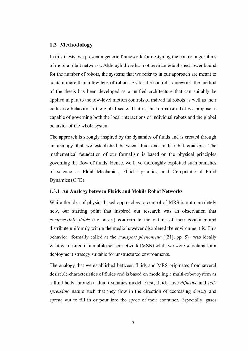
1.3.1 An Analogy between Fluids and Mobile Robot Networks
While the idea of physics-based approaches to control of MRS is not completely
new, our starting point that inspired our research was an observation that
compressible fluids (i.e. gases) conform to the outline of their container and
distribute uniformly within the media however disordered the environment is. This
behavior –formally called as the transport phenomena ([21], pp. 5)– was ideally
what we desired in a mobile sensor network (MSN) while we were searching for a
deployment strategy suitable for unstructured environments.
The analogy that we established between fluids and MRS originates from several
desirable characteristics of fluids and is based on modeling a multi-robot system as
a fluid body through a fluid dynamics model. First, fluids have diffusive and self-
spreading nature such that they flow in the direction of decreasing density and
spread out to fill in or pour into the space of their container. Especially, gases

6
diffuse into the space and achieve homogeneous density distribution over the
environment regardless of its complexity. This is a very favorable behavior in
challenging terrains for multi-robot surveillance systems and mobile sensor
networks which are required to maximize coverage while preserving uniformity.
Another very important property of fluids is that any flow variation or disturbance
in one part of the fluid affects the rest by propagation. Thus, when a fluid body is
considered as a collection of infinitesimal fluid elements, this behavior points out
the presence of some kind of a coordination mechanism among these elements.
Reflection of this behavior in a multi-robot system, if modeled as a fluid, can
possibly feature the same coordination mechanism among robots and equip them
with the expected collective reactivity. Similarly, there are more of these features
of fluids that favor a fluid dynamics framework as we explain in detail later.
1.3.2 Smoothed Particle Hydrodynamics: A Meshfree Particle Method
Fluid Dynamics deals with the flow of fluids and is based on the mathematical
statements of three fundamental physical principles : Conservation of mass,
momentum, and energy. By applying these principles to a fluid model, the
governing equations of fluid dynamics are obtained. However, these equations are
not analytically solvable in general and require the employment of computational
methods. Among these computational methods, Smoothed Particle Hydrodynamics
(SPH) is a meshfree particle method that models a fluid body as a collection of
moving particles and numerically analyzes the flow equations in these particle
locations. It recently became commonly used in fluid simulations and is very
suitable for distributed and parallel computations.
It is the meshfree particle nature of SPH that it can very suitably be implemented
within a distributed system of mobile agents. Apparently, a fluid particle in SPH
corresponds to a robot in our framework and the governing flow equations are
numerically solved by each robot in its locality.

7
1.3.3 A Framework for Control of Robot Networks
Behaviors of fluids that inspired our model differ from one fluid to another and
depend on some physical properties of the particular fluid and media. For example,
a gas flows somewhat differently than a liquid as a result of different physical
descriptions of the pressure distribution. Or a viscous1 fluid appears to be less
viscous under higher temperature conditions. More importantly, the environment
in which the fluid flows largely determines the overall shape of the flow. There are
a lot of similar parameters that distinguish a particular flow from one another and
result in quite different flow patterns.
The idea in our approach is to utilize these parameters to generate a desired motion
of the robots both in the local and global scales as we are free to choose any setting
for modeling our multi-robot system as an artificial fluid body. Even we can
introduce unphysical values to these parameters whenever it comes favorable.
Therefore, the collective behavior of the system can be controlled through a set of
parameters that directly govern the flow both in the local and global scale. The
framework that we propose separates the two basic behavior control levels, local
(low level) and global (high level), of a robot by identifying a set of model
parameters in between so that the high level controller can be designed
independently of the underlying low level fluid dynamics model. The parameters
are such that the dynamic behavior of the robots both in the local and global scale
can be controlled by assigning them appropriate values.
1.3.4 Desirable Characteristics of the Proposed Approach
Since SPH is a meshfree particle method, it can be implemented in a distributed
multi-agent system whose members correspond to artificial fluid particles. Hence,
the approach provides an inherent decentralization. The governing equations of
fluid dynamics are adapted and applied to MRS such that each robot
computationally solves them to find out its own velocity control inputs.
1 Viscosity refers to the resistance of the fluid to flow due to friction

8
Decentralized nature of our SPH implementation also ensures that the control
algorithm is scalable with the number of robots as it is independently run by each
individual. Similarly, decentralization benefits to the robustness of the approach as
well because centralized or hierarchical algorithms suffer from partial failures that
may result in the overall failure of the system.
Finally, another very important aspect of our fluid physics-based approach is that
the behavior of a multi-robot system governed by this method can be
macroscopically modeled and predicted. This is among the current issues in large-
scale MRS, especially in swarm robotics [22].
1.3.5 Contributions of the Thesis
In this thesis, we propose a novel model that enables us to control emergent
aggregate behaviors of collective multi-robot systems within a unified framework.
We base our formalism on the physics of fluids through some analogies that we
established between multi-robot systems and fluid bodies as well as individual
robots and fluid particles. Our formalism exploits SPH as a distributed
computational method that each robot runs in its algorithm. Our control
methodology leads us to achieve desirable properties such as decentralized
coordination, scalability, and robustness by applying the physical principles behind
the dynamics of fluids to the distributed control of robots.
Contributions of the thesis may be summarized as follows:
a. The idea of designing the low level, reactive behavior controller of a robot
in terms of both local control parameters and global (collective) control
parameters is novel among physics-based approaches to control of multi-
robot systems. The fluid dynamics framework that we proposed well serves
this idea since we model individual robots as fluid particles that are parts of
a fluid body and inherit the global properties of the whole body. That is,
robots possess local properties of their own as well as global properties that
are common to all others.
9
b. To the best of our knowledge, our work is the first approach that
establishes a comprehensive analogy between fluids and multi-robot
systems and explicitly models them as fluids using ‘Fluid Dynamics’. It
thoroughly adapts and exploits the mechanisms available in the physical
and mathematical description of fluids and fluid flow towards developing a
framework for control of large-scale multi-robot systems.
1.3.6 Outline of the Thesis
In Chapter 2, a review of the previous work on various approaches to the collective
control of MRS is provided with a special emphasis on physics-based methods.
Chapter 3 presents a discussion on essential concepts in fluid dynamics and
smoothed particle hydrodynamics. Our proposed control approach is formalized in
Chapter 4. Then in Chapter 5, experimental validation of the method is elaborated
through simulations and the results are discussed. Finally, the thesis is concluded
in Chapter 6. Appendices provide detailed discussions on the material and give the
conference publications produced out of this work.
10
CHAPTER 2
LITERATURE SURVEY: CONTROL OF MULTI-ROBOT SYSTEMS
Before discussing the previous works of the literature that share some common
features with the proposed method, it would be beneficial to assort the approaches
to the control problem in general. According to the commonly adopted
classification in the literature [23]-[25], types of robot control can be categorized
in four classes as follows:
a. Reactive Control: As a control technique characterized by the tight
coupling between sensory inputs and effector outputs, reactive control is
especially suitable for tasks that require fast dynamic reactivity to changing
environmental conditions without much cognitive reasoning. However, it is
limited by the lack of internal representations of the world and of learning
capability over time.
b. Deliberative Control: In contrast to reactivity, deliberative control uses all
sensory inputs and internal knowledge to plan for the next action. Since
planning is a computationally complex and time consuming process, this
type of control typically suffers from slow responsiveness.
c. Hybrid Control: As a strategy that aims at benefiting from the desirable
characteristics of both reactive and deliberative control, the hybrid scheme
combines the real-time features of reactivity with the reasoning and
planning capability of deliberation. In order for interaction and coherence
among these two controls, an intermediate component is required.
d. Behavior-Based Control: Inspired from the interactions of animals with
their environments, behavior-based approaches define a set of behaviors
starting from low-level primitive actions to more complex task behaviors.
They are organized in a bottom-up fashion and executed in parallel.

11
Behavior-based systems encompass reactivity, while they also store
internal world representations and knowledge as a network of
interconnected behaviors. Unlike the layers in hybrid control, these
behaviors do not substantially differ in terms of their representation.
Since the study of multi-robot systems inherits much of its properties from single-
robot studies, control approaches to multi-robot systems (MRS) can also be
classified according to the above definitions. Among these, behavior-based control
approaches dominate cooperative MRS research [26]-[31].
Apart from the behavior-based MRS, there is an emerging field in collective
robotics research called swarm robotics. According to the definition in [6],
Swarm robotics is the study of how large number of relatively simple physically embodied agents can be designed such that a desired collective behavior emerges from the local interactions among agents and between the agents and the environment.
Researches in swarm robotics are commonly inspired by ethological phenomena in
which swarms of animals (insects, fishes, birds, etc.) interact to coordinate their
actions, create collective intelligence, and perform tasks that are far beyond the
capabilities of individual members. Absence of central control in these behaviors
and emergence of cooperation from only local interactions makes social swarms
highly fault-tolerant, scalable, and adaptive to changing conditions. It is these
inherent properties of biological swarms, which are also desirable for collective
robotics, that attract a growing interest among researchers. Swarm robotics
techniques currently available in the literature base their formalism on the
underlying biological phenomena, trying to mimic the behaviors of animals in
simulated or embodied artifacts. In these studies, adaptation of animal behaviors to
multi-robot systems as a low-level coordination mechanism is mainly addressed.
In this respect, swarm robots can be characterized as highly reactive.
2.1 Classifying the Proposed Method
Since the previous work on the general control approaches is abound, we will limit
our concern in this survey to those exhibiting considerable commonality with the

12
proposed method. In order to do that, we will first classify the fluid dynamics
framework.
As will be clearer in the following chapters, the proposed method can be
characterized by the following features:
a. Layered Architecture: The proposed method describes a framework in
which there are two basic layers of control. One is a reactive low-level
control layer that introduces the fluid dynamics model. Low-level controls
of the robots in the system are based on local interactions of fluid elements
and governed by computationally simple equations that allow the robots to
respond to dynamical changes in the environment. This reactive layer of
control also provides a set of parameters belonging to the model in this
layer that can be used by high-level behaviors to accomplish global tasks.
In this respect, the control architecture is also suitable for hybrid and
behavior-based approaches such that internal world representations, task
planning layers or learning algorithms can be incorporated into the
architectural framework.
b. Decentralized: Each robot in the system determines its own behavior
according to its instantaneous knowledge of the local environment and of
neighbors obtained through local sensing and communication, and to its
collective behavior scheme preprogrammed at design-time. Yet, the set of
model parameters mentioned above enable centralized realizations in
which the collective behavior scheme may be detached from individual
robots and concentrated in a central controller unit.
c. Homogeneous: Basically, each robot is considered to be equal in terms of
physical properties as a fluid body is composed of identical elements.
However, differences may easily be introduced into the model of any robot.
While physical difference results in behavioral variation, it can also be
obtained by specifying a different collective behavior scheme for any
particular robot. Hence, operational heterogeneity may be obtained in two
ways.

13
2.2 The Artificial Potential Field (APF) Approach
The artificial potential field approach has long been popular in mobile robotics
area starting from the initial work of Khatib [32], and producing a vast amount of
research onwards. It has been largely applied to obstacle avoidance [33], path
planning [34], [35], and navigation [36] problems for single-robot systems. For
multi-robot systems, in addition to the previous areas, the APF approach is utilized
primarily in deployment control [37] and formation control [38], [39].
The principle idea behind APF approach is that the environment in which the
mobile robot moves is modeled as a 2D domain of a potential function and that the
motion of the robot is governed by a virtual force field (VFF) derived from this
potential field so that the robot moves to a point with minimum potential value. In
this potential, areas of obstacles take high values and target points or desired paths
take locally minimum values. Therefore, the direction of motion is opposite to the
gradient of the potential field.
The reason for the popularity of the APF approach is its simplicity and elegance
such that it can easily be implemented either off-line or online without much
computational burden. Hence, it is effective in real-time applications. However, it
also suffers some shortcomings inherent to its pure form. There are 3 major
problems identified by [40] as follows:
a. Local Minima: The robot may trap into undesired local minima such as U-
shaped dead ends due to obstacles. Trap situations have been remedied by
using heuristic methods in expense of non-optimal paths or by global path
planners that require global information.
b. No Passage between Closely Spaced Obstacles: When a robot attempts to
pass through two closely spaced obstacles, the repulsive forces from the
obstacles may result in a combined force which is equal in magnitude and
opposite in direction to the force applied by the target, ceasing the motion
of the robot.

14
c. Oscillations in presence of obstacles and in narrow passages: Due to the
strong dependency of the force field to the nearby obstacles, the APF
method tends to cause unstable motion in presence of obstacles.
Although the state of the art has largely resolved the abovementioned problems
[41], the APF approach is a reactive control technique which can merely be
utilized as a low-level behavior for motion control of either single or multiple
mobile robots. However, it does not incorporate any mechanism for integrating it
into a unified control architecture designed for collective robotics, in which all
levels of control, from the lowest to the highest, should involve aspects of
collective control. For example, local reactive behaviors should be controllable by
high-level behaviors and each local interaction should also serve the global task.
2.3 Fluid Physics Based Approaches
Nature has always been a source of inspiration for researchers in creating new
ideas for problems of science and engineering. Robots, as being one of the most
advanced artifacts, also benefited from innumerable examples available in nature.
Approaches that originate from the laws of physics to robot control problems are
inspired by the profound mechanisms of matter. Contrary to probabilistic or
heuristic methods employed in the biologically-inspired swarm approach, physics-
based approaches exploit well-established grounds of related physics areas such as
fluid mechanics, electrostatics, and material formations.
In this section, we concentrate on fluid physics-based approaches that have already
been used for various mobile robotics problems. We identified two main topics in
which fluid metaphors have been utilized. These are path planning for single-robot
systems and deployment, coverage, and formation control for multi-robot systems.
2.3.1 Robot Path Planning using Stream-Fields
The path generation and navigation problem of mobile robots was first addressed
using a fluid dynamics method by Keymeulen and Decuyper in [42], [43], where
they used the stream field method as a path generator to plan local-minima-free
and optimal paths for an autonomous mobile robot. Considering indoor and maze-

15
like environments, they generated the path of the robot by modeling it as a fluid
particle flowing under the effect of a fluid pump at the starting point and an outlet
at the destination. The equation that describes the flow of fluid is called the
Laplace equation and the solutions are formally called harmonic functions. The
most important property of harmonic functions is that they are free from local
extrema. Thus, the robot does not get trapped in vicinities of obstacles as is the
case in ordinary potential function approaches. Similarly, [44] used harmonic
functions for obstacle avoidance and path planning, besides the panel method from
computational fluid mechanics to represent arbitrarily shaped obstacles. While
these approaches can adapt to dynamical changes of the environment, the
constrained dynamic equation of flow is solved by a central planner which requires
global knowledge of the environment in question. The panel method also needs
global information to fit panels to obstacle surfaces. Therefore, stream field or
harmonic function based methods are not suitable for multi-robot systems
operating in incompletely known environments.
In a more recent work in [45], one of the first attempts was made to utilize a more
general, if not the most, fluid dynamics equation called Stokes equation. In this
work, applications in uneven outdoor terrain conditions are targeted with an
emphasis on the effect of viscosity and external body forces. Viscosity is modeled
as a virtual interaction between the robot and the surrounding environment so that
collision-free paths are found in expense of sub-optimality around obstacles.
External forces, on the other hand, are used to account for the real effect of friction
between robot tires and the ground. However, the world under consideration is
again fully known and discretized by a global planner, which cannot be applied as
a scalable approach for distributed multi-robot systems in unknown environments.
2.3.2 Fluid Models for Controlling Robot Networks
The idea of incorporating the fluid dynamics equations into the control strategy of
a multi-robot system was first introduced by Zarzhitsky et al. [46], [47]. The
problem was to trace a chemical plume back to its source using a team of mobile
robots. Since the plume itself is a fluid, its flow is governed by the fluid dynamics

16
equations. The essence of this method is that when the mobile robot team is
considered as a mesh for measuring the density of the plume and computationally
solving for the velocity field of the fluid around the robots, the velocities of the
robots can be controlled to head toward the opposite direction to the flow, which
eventually leads to the source of the plume. However, in order to organize the
robots in a computational mesh formation, additional control is required, for which
the authors utilized a previously proposed artificial physics framework [48].
Basically, this approach is inspired by the dynamics of fluids whereas it is not the
multi-robot system itself modeled as a fluid but a chemical plume that is traced. In
other words, the multiple robot system merely computes the velocity of the plume
and controls the velocity of robots such that they trace the plume back to its
source. Therefore, the method is not applicable to other problems that do not
involve a fluid to guide the motion of the multi-robot system.
Another work partly by the same authors in [49] and [50] proposes to use the
kinetic theory (KT) of gases to model swarm robots as gas particles to obtain the
coverage and obstacle avoidance characteristics of gases in a multi-robot system.
While the motivation of the authors in using a gas model for a multi-robot system
partly overlaps with our aims, KT is a fundamentally different formalism for
modeling gases than the fluid dynamics model we use. In the kinetic theory of
gases, fundamental laws of nature are applied directly to atoms and molecules, and
the average behaviors and properties of the gas are found by using statistical
analyses techniques because of the very large number of particles (typically on the
order of 1019/cm3). For instance, the fact that “locations of individual particles are
unpredictable” is stated as a desirable characteristic of a multi-robot system.
However, we believe that we should be able to predict the locations of individual
robots as much as possible in a multi-robot system in order to effectively control
their cooperative behavior. Also, the kinetic theory suggests that the particles are
in constant and random motion such that they constantly collide with each other
and with the walls of their container in a perfectly elastic way. However, neither
random motions nor constant collisions are desirable in multi-robot systems even

17
if they can result in a macroscopically gas-like behavior. Therefore, the kinetic
theory approach to modeling and controlling MRS is not suitable.
The most relevant work of the literature to our proposed method is the study of
Perkinson and Shafai [51] that proposes to control the positional organization and
movement of a robotic swarm based on Smoothed Particle Hydrodynamics (SPH).
It considers robots as particles in SPH and directly applies the formulation of SPH
to simulated robots in 2D. While this work represents the first attempt to utilize
SPH for modeling the low-level behavior of a multi-robot system, it does not
establish an analogy between fluids and large-scale multi-robot systems. Hence, it
lacks conceptual adaptations of concepts in fluid physics to swarm robotics. Also,
this work only addresses the coverage problem using a gas-like fluid model in
bounded environments. Thus, the real potential of the SPH approach in terms of
describing the low-level behavior model of a robot swarm is not demonstrated.
2.4 Deployment of Mobile Sensor Networks
Mobile sensor networks have recently emerged as a new technology integrating
various fields such as sensor fusion, wireless ad-hoc communication, and
distributed robotics. The basic idea of mobile sensor networking is to deploy smart
sensor nodes ‘en masse’ within an environment for surveillance, data mining, and
search. Although initially the main drive of research on sensor networks was
military [9], civil applications have also found new emphases by technological
improvements.
One of the most fundamental concepts in sensor networking is coverage. It is the
quality-of-service that a network can provide [52] and may be defined by the
percentage of the surveillance area that is sensed through sensor nodes. Coverage
is strongly dependent on ‘deployment’ of the sensor network over the
environment. Therefore, terrain and task coverage for efficient surveillance and
mission realization stemming from effective deployment are critical control
problems to be dealt with. Also, the challenges posed by large-scale mobile sensor
networks in unknown, unstructured, and hostile environments necessitate the
18
utilization of distributed self-deployment schemes, in which deployment is an
emergent behavior of the local coordination among sensor nodes.
The previous works in the literature commonly describe a potential-field-based
approach to deployment, in which nodes are treated as virtual particles, subject to
virtual forces. These forces repel nodes from each other and from obstacles, and
ensure that from an initial compact configuration, nodes will spread out to
maximize the coverage area of the network [37], [52]-[56]. In these algorithms,
deployment is conceived as a coverage process that maneuvers the sensor nodes
from an initial random or compact configuration to a suboptimal configuration in
which a static equilibrium is attained and coverage requirements are met. Although
these approaches assume an unknown sensing environment, all of them implicitly
assume prior information about the surveillance area’s physical range by
considering the deployment of a predetermined and fixed number of sensor nodes.
When the nodes disperse sufficiently over the environment, the network reaches
static equilibrium and a certain level of area coverage is achieved. However, if the
size of the surveillance environment is not known a priori, these algorithms can
only provide coverage to the size extent of the area that is previously fixed by the
number of nodes to be deployed. Thus, a certain quality of service could not be
guaranteed with these approaches.
2.5 Publications of the Proposed Method
In our previous publications [57]-[59], we presented the first fluid dynamics-based
model as a distributed, scalable, and robust solution to the deployment problem of
mobile sensor networks. We extended the idea of physics-inspired approaches by
modeling a robot network as a fluid body and controlling the deployment process
through the parameters available in the governing equations of fluid dynamics. We
used a custom defined meshfree particle method for the numerical solution of the
equations. Primarily addressing the coverage of unknown unstructured
environments with mobile sensor networks, we demonstrated how the
configuration of the network can be changed to satisfy connectivity requirements

19
and analyzed the robustness of the approach in response to dynamical environment
and network conditions.
In a following paper [60], we further extended our previous formalism by
developing a low-level, fluid dynamics based control model to coordinate the local
interactions of robots while providing an interface composed of flow parameters to
higher level algorithms for controlling the global behavior of the system. We
exploited SPH for the modeling and analysis of robot swarms through the set of
fluid dynamics equations. We demonstrated the validity and promise of the
approach by applying it to common problems recurring in the MRS literature.
The abovementioned publications can be found in Appendix B. While Chapter 4
will provide all in-depth details of the proposed method of this thesis, primarily we
prefer in the next chapter to overview the mathematical background necessary for
understanding the basis of the fluid dynamics based methodology that we
developed for controlling collective robot networks.

20
CHAPTER 3
ESSENTIALS ON FLUID DYNAMICS
In this section, a brief overview of and some essential material on fluid dynamics
and smoothed particle hydrodynamics (SPH) are presented for a better
understanding of the proposed approach in the next chapter. The overview here on
fluid dynamics and SPH follows from the references in [61] and [62], respectively.
The reader is advised to consult these references for further details and discussions
of all concepts and equations that are present in this chapter.
3.1 Basic Fluid Dynamics Concepts
Before deriving the governing equations of fluid dynamics, we need to identify
some background concepts related with the notion of fluid flow and fluid
dynamics. Basically, there are two types of fluids, namely gases and liquids. Gases
are compressible while liquids are incompressible. Fluid dynamics is based on the
mathematical statements of three fundamental physical principles:
a. Mass is conserved.
b. Newton’s second law, F = ma.
c. Energy is conserved.
The governing equations of fluid dynamics are derived by applying these physical
principles to a suitable model of the fluid flow. However, definition of a suitable
model of the flow is not a trivial consideration. There are four models of flow as
described in the next part.
3.1.1 Finite Control Volume and Infinitesimal Fluid Element
Unlike a solid body, a fluid is a deformable substance and in motion the velocity
of each part of the fluid may be different. Therefore, instead of looking at the
whole flow field at once, we should limit our attention to a finite region of the
fluid. In finite control volume approach, this region is called a control volume V

21
along with a control surface S bounding this volume (see Figure 1 (a) and (b)).
The control volume may be fixed in space with the fluid moving through it as in
Figure 1 (a). Alternatively, the control volume may be moving with the fluid such
that the same fluid particles are always inside it (Figure 1 (b)). In either case, the
control volume is a reasonably large, finite region of the flow. The fundamental
physical principles are applied to the fluid inside the control volume and to the
fluid crossing the control surface.
Alternatively, we can model the flow using an infinitesimally small fluid element
with a differential volume dV as well (see Figure 1 (c) and (d)). Again, the fluid
element may be fixed in space or it may be moving along a streamline with a
velocity vector V equal to the flow velocity at each point of the field, as in Figure
1 (c) and (d), respectively. Then, the fundamental physical principles are applied
just to the infinitesimally small fluid element itself.
The governing equations obtained by applying the fundamental physical principles
to either the control volume or the infinitesmal fluid element fixed in space are
called the conservation form of the governing equations. On the other hand, the
equations obtained from the control volume or infinitesmal fluid element moving
with the fluid are called the nonconservation form of the governing equations.
In the analysis of fluid dynamics, one among the four flow models described
above may be more preferable over the others due to a specific computational
convenience of the model. Within the perspective of our particular application
purposes that will be described in the next chapter, we will utilize the model of
infinitesimal fluid element moving with the flow field.

22
Figure 1 Models of a flow
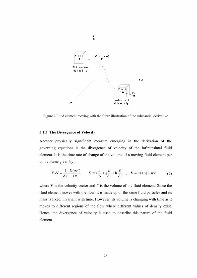
3.1.2 Substantial Derivative
When the model of infinitesimal fluid element moving with the flow (Figure 1 (d))
is adopted, a conventional notation called the substantial derivative D/Dt comes
into play to denote the time rate of change (of some physical quantity) following a
moving fluid element. That is, for a fluid element in Cartesian space as shown in
Figure 2, the instantaneous time rate of change of density as the fluid element
moves through Point 1 is denoted by Dρ/Dt and is computed as
zw
yv
xu
tDtD
DtD
tttt ∂∂
+∂∂
+∂∂
+∂∂
≡≡−−
→,lim
12
12
12
ρρρ (1)
The physical significance behind substantial derivative is that the time rate of
change of density or some other physical quantity of a given fluid element as it
moves through space results from not only the transient fluctuations of the flow
field at a fixed point but also from the change due to the movement of the fluid
element from one location to another in the flow field where the physical
properties are spatially different.
23
Figure 2 Fluid element moving with the flow: illustration of the substantial derivative
3.1.3 The Divergence of Velocity
Another physically significant measure emerging in the derivation of the
governing equations is the divergence of velocity of the infinitesimal fluid
element. It is the time rate of change of the volume of a moving fluid element per
unit volume given by
1 ( ) , ,D V u v wV Dt x y z
δδ
∂ ∂ ∂∇ = ∇ ≡ + + = + +
∂ ∂ ∂iV i j k V i j k (2)
where V is the velocity vector and V is the volume of the fluid element. Since the
fluid element moves with the flow, it is made up of the same fluid particles and its
mass is fixed, invariant with time. However, its volume is changing with time as it
moves to different regions of the flow where different values of density exist.
Hence, the divergence of velocity is used to describe this nature of the fluid
element.

24
3.2 The Governing Equations of Fluid Dynamics
In this section, the equations obtained from the three fundamental conservation
principles are shortly discussed. We provide them in the following parts without
their derivations, for which the reader is referred to the second chapter of the
reference in [61].
3.2.1 The Continuity Equation
Having determined a model of the flow, the physical principles constituting the
foundation of fluid dynamics may now be applied to the model. The continuity
equation is derived from the application of the first principle, namely the
conservation of mass. For the model of an infinitesimal fluid element, the
conservation of mass principle states that the time rate of change of mass of the
fluid element is zero as the element moves along the flow. With the help of the
statements of substantial derivative and divergence of velocity, the continuity
equation turns out to be
: 0DContinuity EquationDtρ ρ+ ∇⋅ =V (3)
3.2.2 The Momentum Equation
A moving fluid element experiences various kinds of forces. These forces are
categorized into two and called as either body forces or surface forces. Examples
to body forces are gravitational, electric, and magnetic forces. Surface forces, on
the other hand, are due to the pressure distribution acting on the surface of the
element or due to the viscous friction and shear stresses imposed by the
surrounding fluid media.
A fluid element under the effects of these forces obeys another physical law;
Newton’s second law. The governing equations obtained by applying this principle
to a model of viscous flow, in which the transport phenomena of friction and
thermal conduction are included, are called the Navier-Stokes Equations. In these
equations (4), p is the pressure distribution acting on the surfaces of the fluid
element and f stands for the body force per unit mass. τ represents the normal

25
stress, which is related to the time rate of change of volume of the fluid element,
when its subscripts are the same (e.g. τxx) or the shear stress, which is related to the
time rate of change of the shearing deformation of the fluid element, when it
subscripts are different (e.g. τxy).
:
:
:
yxxx zxx
xy yy zyy
yzxz zzz
Du px momentum fDt x x y zDv py momentum fDt y x y zDw pz momentum fDt z x y z
ττ τρ ρ
τ τ τρ ρ
ττ τρ ρ
∂∂ ∂∂− = − + + + +
∂ ∂ ∂ ∂∂ ∂ ∂∂
− = − + + + +∂ ∂ ∂ ∂
∂∂ ∂∂− = − + + + +
∂ ∂ ∂ ∂
(4)
For newtonian2 fluids, viscous components of the Navier-Stokes equations are
formulated as follows.
( )
( )
( )
2 ,
2 ,
2 ,
xx xy yx
yy xz zx
zz yz zy
u v ux x y
v u wy z x
w w vz y z
τ λ μ τ τ μ
τ λ μ τ τ μ
τ λ μ τ τ μ
⎛ ⎞∂ ∂ ∂= ∇ + = = +⎜ ⎟∂ ∂ ∂⎝ ⎠
∂ ∂ ∂⎛ ⎞= ∇ + = = +⎜ ⎟∂ ∂ ∂⎝ ⎠⎛ ⎞∂ ∂ ∂
= ∇ + = = +⎜ ⎟∂ ∂ ∂⎝ ⎠
i
i
i
V
V
V
(5)
Here, μ is the molecular viscosity and λ is the second viscosity coefficient. These
two characteristic constants of a fluid are related by the following identity.
23
λ μ= − (6)
3.2.3 The Energy Equation
The third physical principle is the conservation of energy or equivalently the first
law of thermodynamics. Considering again an infinitesimal fluid element moving
with the flow, it states that the rate of change of energy inside the fluid element is
equal to the sum of the net flux of heat into the element and the rate of work done
on the element due to body and surface forces. In the energy equation given below, 2 For newtonian fluids, shear stress is proportional to the time rate of change of the strain, i.e. velocity gradients. Mostly, common fluids are newtonian.

26
e is the internal and V 2/2 is the kinetic energy of the fluid element. On the right
hand side, q is the volumetric heat addition per unit mass and f is the body force
vector.
( ) ( ) ( )
( ) ( ) ( )
( ) ( ) ( )
( ) ( ) ( )
2
2
yxxx zx
xy yy zy
yz zzxz
D V T T Te q k k kDt x x y y z z
up vp wpx y z
uu ux y z
v v v
x y z
w wwx y z
ρ ρ
ττ τ
τ τ τ
τ ττρ
⎛ ⎞ ⎛ ⎞∂ ∂ ∂ ∂ ∂ ∂⎛ ⎞ ⎛ ⎞+ = + + +⎜ ⎟ ⎜ ⎟⎜ ⎟ ⎜ ⎟∂ ∂ ∂ ∂ ∂ ∂⎝ ⎠ ⎝ ⎠⎝ ⎠⎝ ⎠∂ ∂ ∂
− − −∂ ∂ ∂
∂∂ ∂+ + +
∂ ∂ ∂
∂ ∂ ∂+ + +
∂ ∂ ∂
∂ ∂∂+ + + + ⋅
∂ ∂ ∂f V
(7)
3.2.4 Some Comments on the Governing Equations
The three equations –continuity, momentum, and energy– discussed so far
represent the complete set of governing fluid dynamics equations. They are a
coupled system of nonlinear partial differential equations and are very difficult to
be solved analytically. Actually, there is no general closed-form solution to these
equations yet.
While these equations completely describe the flow of a fluid, they involve some
variables such as pressure and internal energy that require additional relations be
established. For a perfect gas, for example, the equation of state determines the
relationship between the density of the gas and its pressure as follows.
p RTρ= (8)
In this equation, R is the specific gas constant (8.314472 m3.Pa.K-1.mol-1) and T is
the absolute temperature. Similarly, for a calorically perfect gas, the caloric
equation of state is defined as
ve c T= (9)
27
where cv is the specific heat at constant volume.
3.2.5 The Boundary Conditions
The equations discussed so far are the same governing equations of flow for a fluid
whatever its particular environmental conditions are. Then, the real driver for any
particular solution is the boundary conditions and initial conditions introduced by
the environment. For example, for a viscous flow, the boundary condition on a
surface dictates a zero relative velocity between the surface and the fluid
immediately at the surface (V = 0). This is also called as the no-slip condition. A
similar condition is prevalent for the temperature necessitating a thermal
equilibrium at the surface. For an inviscid flow, there is no friction to promote a
vanishing relative velocity at the surface. Hence, the flow velocity at a wall may
be a finite, nonzero value. The only boundary condition for an inviscid flow is that
the flow velocity vector immediately adjacent to the wall must be tangent to the
wall. Given the normal vector n of the surface at a point and the flow velocity
vector V at that point, this boundary condition may be formulated as 0⋅ =V n .
Besides the physical boundary conditions, depending on the particular problem at
hand, there may be other initial conditions in the flow elsewhere from the surfaces.
For example, at the inlet of a duct, the pressure of the fluid may at a certain value.
3.3 Computational Fluid Dynamics (CFD)
As stated earlier, the governing equations of fluid flow are a system of nonlinear
partial differential equations, and to date no closed-form solution to these
equations has been found. It was the experimental fluid dynamics that had been
used as the workbench of the theory until the advent of high speed digital
computers combined with accurate numerical algorithms for solving physical
problems. This has revolutionized the way people study and practice fluid
dynamics and introduced a fundamentally new approach –the approach of
computational fluid dynamics.
CFD is based on the replacement of the integrals or derivatives in the governing
equations with discretized algebraic forms, which in turn are solved to obtain
28
numbers for the flow field values at discrete points in space and time. The
arrangement of these discrete points in space throughout the flow field is called a
grid and its determination called as grid generation is a significant consideration in
CFD. In terms of the type of the grid being used, there are two fundamental frames
for describing the process of applying the numerical method. One is the Eulerian
description which is a spatial description and typically represented by the finite
difference method (FDM). It defines a stationary grid over the domain and the
simulated fluid flows across the grid points or mesh cells. The other is the
Lagrangian description which is a material description and typically represented
by the finite element method (FEM). Contrary to the Eulerian grid, Lagrangian grid
is attached to the material and flows with it through the numerical process.
Obtaining the solutions of the governing equations at discrete points in time, on
the other hand, is called a time-marching solution where the dependent flow field
variables are solved progressively in steps of time. Although we will not utilize the
grid-based approach of CFD in our development, time integration techniques of
traditional CFD methods that rely on rectangular grids in two dimensions will be
exploited. Hence, it is worth mentioning one of these techniques –the Lax-
Wendroff technique– in the following part.
3.3.1 The Lax-Wendroff Technique
The Lax-Wendroff technique is an explicit, finite-difference method particularly
suited to marching solutions of an inviscid flow with the unsteady Euler
equations3. The governing equations are rearranged in (10) with the assumption of
no body forces.
3 Euler equations are the simplified form of the Navier-Stokes equations when the flow is inviscid, i.e. dissipative viscosity, mass diffusion, and thermal conductivity are neglected.

29
⎟⎟⎠
⎞⎜⎜⎝
⎛∂∂
+∂∂
+∂∂
−=∂∂
−
⎟⎟⎠
⎞⎜⎜⎝
⎛∂∂
+∂∂
+∂∂
−=∂∂
−
⎟⎟⎠
⎞⎜⎜⎝
⎛∂∂
+∂∂
+∂∂
+∂∂
−=∂∂
yp
yvv
xvu
tvmomentumy
xp
yuv
xuu
tumomentumx
yv
yv
xu
xu
tContinuity
ρ
ρ
ρρρρρ
1:
1:
:
(10)
The solution to each of these equations are obtained using a time-marching
approach; note that the equations are already arranged in a convenient form, with
the time derivatives isolated on the left-hand side and the spatial derivatives on the
right-hand side. The Lax-Wendroff method is predicated on a Taylor series
expansion in time, as follows. Choose any dependent flow variable; for purpose of
illustration let us choose velocity component u. Consider the two dimensional grid
shown in Figure 3. Let tjiu , denote the velocity in x-direction (x-velocity) at grid
point (i,j) at time t. Then, the x-velocity at the same grid point at time t+∆t,
denoted by ttjiu Δ+
, , is given by the Taylor series
( )
+Δ
⎟⎟⎠
⎞⎜⎜⎝
⎛
∂∂
+Δ⎟⎟⎠
⎞⎜⎜⎝
⎛
∂∂
+=Δ+
2
2
2,
2,
,,t
tu
tt
uuu
tji
tjit
jitt
ji (11)
When employing (11), we assume that the flow field at time t is known and (11)
gives the new flow field at time t+∆t. Then in (11), tjiu , is known. The unknowns
on the right-hand side of (11) are the time derivatives of the dependent flow
variable u. According to the required accuracy of the solution, these time
derivatives may be derived by using the governing equations in (11) along with an
increasing elaboration with the degree of accuracy. Generally, Lax-Wendroff
technique is referred to as the second-order-accurate approximation of the time-
marching solution in (11).

30
Fluid Body
dV V
y
x
Infinitesimal Fluid Elements
i-1 i i+1
j
j-1
j+1
Figure 3 Rectangular grid segment and infinitesimal fluid elements
In order for the calculation of the spatial derivatives in (10), the finite difference
method on the rectangular grid shown in Figure 3 is used. For example, the spatial
derivative of tjiu , with respect to x is given by
xuu
xu t
jit
jit
ji
Δ−
=∂∂ −+
2,1,1, (12)
which is called the second-order central difference. Similar difference equations
exist for higher order spatial derivatives and for successive partial derivatives with
respect to different dimensions.
3.4 Smoothed Particle Hydrodynamics (SPH)
Conventional grid or mesh based methods such as Finite Difference Method
(FDM) and Finite Element Method (FEM) have been widely applied in CFD and
currently are the dominant numerical methods to simulate fluid flow. However,
they suffer from some inherent difficulties that limit their applicability to many
problems. First of all, grid-based methods require the generation of an ‘a priori’
mesh over the problem domain. That process is generally not easy at all especially
for complex geometries and may be more computationally expensive than the

31
numerical analysis of the equations itself. The limitations of grid-based methods
are more apparent in existence of special features such as large deformations,
inhomogeneities, and free surfaces. The grid-based methods are also not suitable
for problems where, rather than a continuum of fluid, the concern is on a set of
discrete physical particles such as stars in astrophysics.
In response to these difficulties of grid-based methods, the next generation
computational methods called the meshfree methods emerged. The idea of the
meshfree methods is to provide solutions to integral or differential equations by
using a set of arbitrarily distributed nodes (particles) without using any mesh or
grid to connect them. The particles may be associated with a discrete physical
object or a part of a continuum material and may range from nano scale to
astronomical scale.
Smoothed particle hydrodynamics as a meshfree particle method was originally
invented for modeling astrophysical phenomena in the late 1970’s and then
became popular in the numerical analyses of fluid dynamics problems. SPH has
some special advantages over other grid-based and meshfree methods. For
instance, its formulation is not affected by the arbitrariness of the particle
distribution. Also, SPH is very suitable for the Lagrangian description of the
governing equations as a computational frame moving with the particles and
carrying material properties. The reader is referred to [62] for an in-depth
discussion on SPH.
3.4.1 Particle Approximation in SPH
In SPH, the state of a system is represented by a set of particles that posses
individual particle properties and move according to the governing equations.
Numerical discretization is made by approximating the values of functions,
derivatives, or integrals at particle locations where neighboring particles contribute
to the particle approximations based on their influence on the location. The area of
influence of a particle is defined by a neighboring concept called the support
domain. Basically, the neighbors of a particle lying in its support domain provide
all the necessary information for the field variable approximations at the particle.

32
Figure 4 illustrates the support domain of a particle as an area of a certain radius.
For example, a field variable (e.g. a component of the velocity) u for a particle
located at x = (x, y, z) within the overall problem domain is approximated using
the flow variable information of its neighbors in the support domain as in (13). In
this equation, Ωi is the support of particle i and j represents the neighbors within
this domain. The velocity values of these neighbors are weighted by a shape
function jφ at particle j and summed up.
( ) ( )i
i j jj
u u φ∈Ω
= ∑x x (13)
particle i at x
support domain of particle i: Ωi
Figure 4 Support domain of a particle at x
3.4.2 Basic Formulation of SPH
SPH method was developed for hydrodynamics problems that are basically in the
form of partial differential equations (PDEs) of field variables such as density,
velocity, energy, etc. In order to find numerical solutions to these PDEs, the
problem domain is discretized. Then the function approximation is applied to the
PDEs to produce a set of ordinary differential equations (ODEs) in a discretized
form only with respect to time. Then, this set of ODEs can be solved using one of
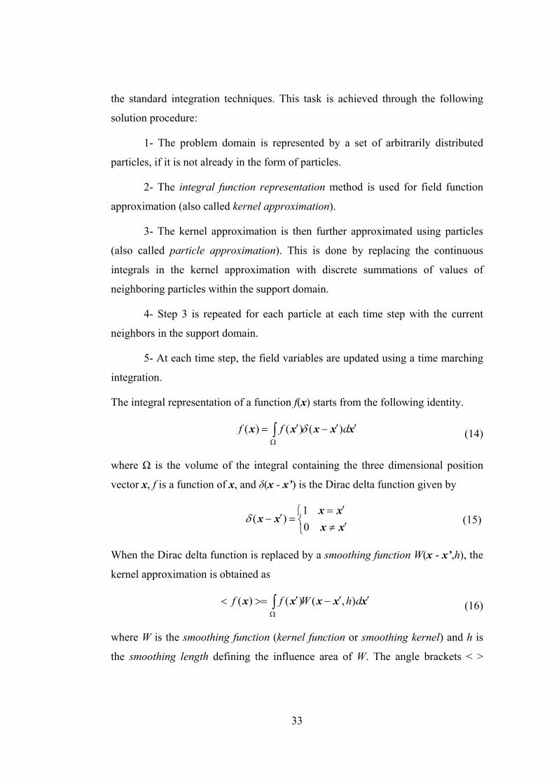
33
the standard integration techniques. This task is achieved through the following
solution procedure:
1- The problem domain is represented by a set of arbitrarily distributed
particles, if it is not already in the form of particles.
2- The integral function representation method is used for field function
approximation (also called kernel approximation).
3- The kernel approximation is then further approximated using particles
(also called particle approximation). This is done by replacing the continuous
integrals in the kernel approximation with discrete summations of values of
neighboring particles within the support domain.
4- Step 3 is repeated for each particle at each time step with the current
neighbors in the support domain.
5- At each time step, the field variables are updated using a time marching
integration.
The integral representation of a function f(x) starts from the following identity.
( ) ( ) ( )f f dδΩ
′ ′ ′= −∫x x x x x (14)
where Ω is the volume of the integral containing the three dimensional position
vector x, f is a function of x, and δ(x - x’) is the Dirac delta function given by
1
( )0
δ′=⎧′− = ⎨ ′≠⎩
x xx x
x x (15)
When the Dirac delta function is replaced by a smoothing function W(x - x’,h), the
kernel approximation is obtained as
( ) ( ) ( , )f f W h dΩ
′ ′ ′< >= −∫x x x x x (16)
where W is the smoothing function (kernel function or smoothing kernel) and h is
the smoothing length defining the influence area of W. The angle brackets < >

34
designate that the integral representation of the function is an approximation unless
W is the Dirac delta function.
Similarly, the kernel approximation for the spatial derivative of a function is
obtained as
( ) ( ) ( , )f f W h dΩ
′ ′ ′< ∇ ⋅ >= − ⋅∇ −∫x x x x x (17)
For the above derivations to be valid, the smoothing function should satisfy certain
conditions as listed below.
1- The smoothing function must be normalized (unity condition) over its
support domain, i.e.
( , ) 1W h dΩ
′ ′−∫ x x x = (18)
2- The smoothing function should be compactly supported (compact
support condition) and positive, i.e.
( , ) 0 for
( , ) 0 for
W h h
W h h
κ
κ
′ ′− = − >
′ ′− ≥ − ≤
x x x x
x x x x(19)
where κ is a constant that defines the non-zero area of the smoothing function with
respect to x. This area defines the support domain of the smoothing function at a
particular location.
3- The smoothing function should be monotonically decreasing with
increasing distance to the particle (decay condition).
4- As the smoothing length approaches to zero, the smoothing function
should approach to Dirac delta function (delta function condition).
0lim ( , ) ( )h
W h δ→
′ ′− = −x x x x (20)
5- The smoothing function should be an even function (symmetry
condition) with respect to a spatial dimension and sufficiently smooth (smoothness
condition).

35
For the particle approximation, the continuous integral representation of the kernel
approximation is converted to a discretized form of summation over all the
particles in the support domain shown in Figure 5.
h
Ωi
rij
i
jW
Figure 5 The support domain for particle i and the 1D projection of a smoothing function over it
The infinitesimal volume dx’ in the kernel approximation is replaced by the finite
volume of the particle ∆Vj, which is related to the particle mass mj as given by
j j jm V ρ= Δ (21)
where ρj is the density of particle j. Using this in (16), the particle approximation
of the function is obtained as
( ) ( ) , ( , )i
ji j ij ij i j
j j
mf f W W W h
ρ∈Ω< >= ⋅ = −∑x x x x (22)
(22) states that the value of a function at particle i is approximated using the
average of those values of the function at all particles in the support domain of
particle i weighted by the smoothing function.
Similarly using (17), the particle approximation of the derivative of the function is
obtained as

36
( ) ( ) ,i
j i j iji j i ij i ij
j j ij ij
m Wf f W W
r rρ∈Ω
− ∂< ∇ ⋅ >= − ⋅∇ ∇ =
∂∑x x
x x (23)
(23) states that the value of the gradient of a function at particle i is approximated
using the average of those values of the function at all particles in the support
domain of particle i weighted by the gradient of the smoothing function.
As for the smoothing function W, there are various choices among which the
Gaussian kernel (Figure 6) is one of the most popular ones due to its smoothness,
stability, and accuracy especially for disordered particles. It is defined as in (24).
Figure 6 The Gaussian kernel and its spatial derivative with κ = h = 2 and xi = (0, 0)
2
2
( , )
1 for 2D ,
Rd
i jd
W R h e
h Rh
α
α π
−=
−= =
x x (24)
3.5 Application of SPH to Navier-Stokes Equations
In this section, application of the SPH method to the governing equations of fluid
dynamics in Lagrangian form will be discussed. The reader is referred to the fourth
chapter of [62] for the details and derivations.
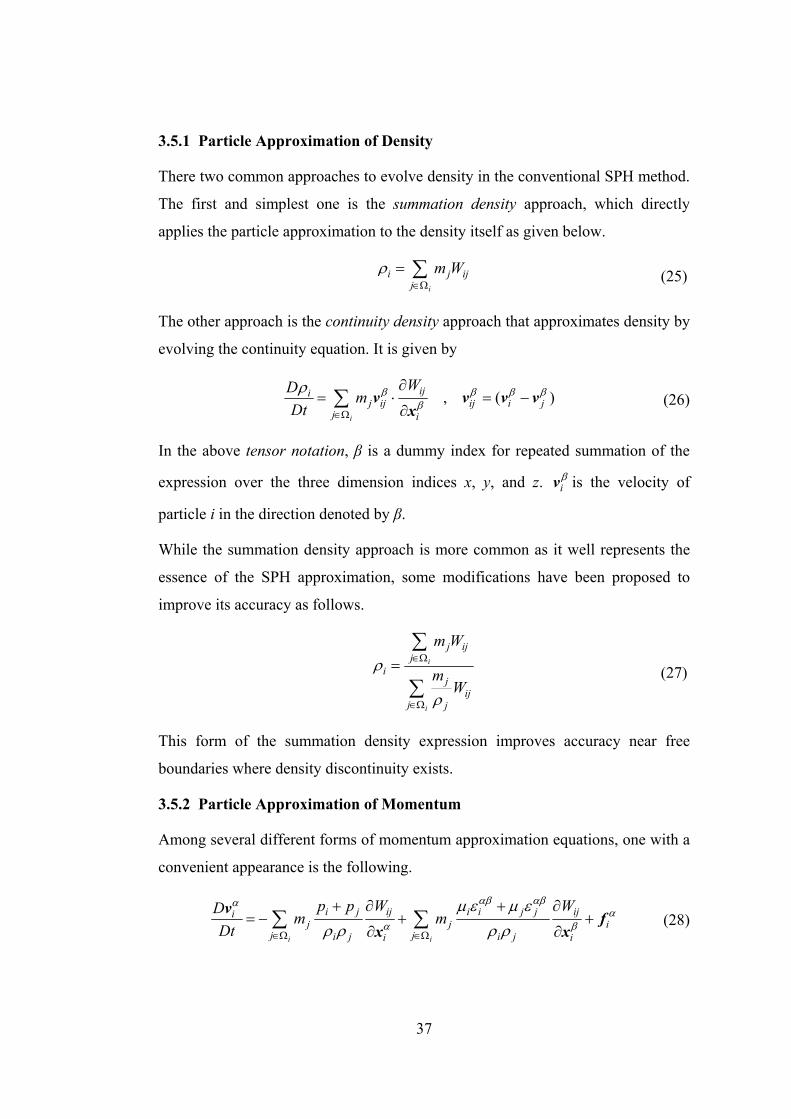
37
3.5.1 Particle Approximation of Density
There two common approaches to evolve density in the conventional SPH method.
The first and simplest one is the summation density approach, which directly
applies the particle approximation to the density itself as given below.
i
i j ijj
m Wρ∈Ω
= ∑ (25)
The other approach is the continuity density approach that approximates density by
evolving the continuity equation. It is given by
, ( )i
ijij ij ij i j
j i
WD mDt
β β β ββ
ρ∈Ω
∂= ⋅ = −
∂∑ v v v v
x(26)
In the above tensor notation, β is a dummy index for repeated summation of the
expression over the three dimension indices x, y, and z. iβv is the velocity of
particle i in the direction denoted by β.
While the summation density approach is more common as it well represents the
essence of the SPH approximation, some modifications have been proposed to
improve its accuracy as follows.
i
i
j ijj
ij
ijj j
m W
mW
ρ
ρ
∈Ω
∈Ω
=∑
∑ (27)
This form of the summation density expression improves accuracy near free
boundaries where density discontinuity exists.
3.5.2 Particle Approximation of Momentum
Among several different forms of momentum approximation equations, one with a
convenient appearance is the following.
i i
i j ij i i j j ijij j i
j ji j i ji i
p p W WD m mDt
αβ αβαα
α β
μ ε μ ερ ρ ρ ρ∈Ω ∈Ω
+ ∂ + ∂= − + +
∂ ∂∑ ∑
v fx x
(28)

38
The first summation on the right hand side of this equation is for the pressure
gradient and the second part is for the viscous force. Another dummy index α
appears here to denote the spatial dimension for which the approximation is made.
The shear strain rate denoted by ε is also given by the following SPH
approximation
23
i i i
j ij j ij ji ji ji ji i ij
j j jj j ji i
m W m W mv v Wαβ β α αβ
α βε δρ ρ ρ∈Ω ∈Ω ∈Ω
⎛ ⎞∂ ∂= + − ⋅∇⎜ ⎟⎜ ⎟∂ ∂ ⎝ ⎠∑ ∑ ∑ v
x x (29)
where δ is the delta function assuming 1 when α=β, or 0 otherwise.
3.5.3 Particle Approximation of Energy
Similar to the momentum, particle approximation of energy also has several
different forms. The one below is a popular one.
12 2
i
i j iji ij ij i i
j i j ii
p p WDe m vDt
β αβ αββ
μ ε ερ ρ ρ∈Ω
+ ∂= +
∂∑ x
(30)
3.5.4 Numerical Issues: Artificial Viscosity and Compressibility
Artificial viscosity was originally proposed to model shock waves, where kinetic
energy is transformed to heat energy, as a form of viscous dissipation. It provides a
damping on the numerical oscillations and help to diffuse sharp variations in the
flow. The most widely used artificial viscosity definition is given below.
( ) ( ) ( )
2
2 2
0
0 0
, ,
1 1 1, ,2 2 2
ij ij ijij ij
ijij
ij ij
ij ij ijij ij i j ij i j
ij
ij i j ij i j ij i j
A c B
h
c c c h h h
φ φρ
φϕ
ρ ρ ρ
Π Π⎧− +⋅ <⎪
Π = ⎨⎪ ⋅ ≥⎩⋅
= = − = −+
= + = + = +
v x
v x
v xv v v x x x
x
(31)
In these equations, A and B are constants typically set around 1. φ = 0.1hij is
inserted to prevent numerical divergence when two particles are too close to each
other. c and v are the speed of sound and the velocity vector of the particle,

39
respectively. Basically, the part associated with A produces bulk viscosity, which
is not necessary if the second part in (28) is used, and the part associated with B
suppresses particle interpenetration at high mach4 numbers. Artificial viscosity is
incorporated into the governing equations as an additive term in the summation in
(28).
In the momentum equation, gradient of the pressure is the main driving entity of
the flow. For compressible fluids, pressure is a function of density and temperature
through the state equation of gases. Hence, it can easily be incorporated into the
numerical analysis. For incompressible fluids, however, density is theoretically
constant and a discrete approximation of density –either through particle method,
FDM, or FEM– results in prohibitive numerical difficulties (e.g. extremely small
time steps) when the actual state equation of liquids are used. The fact that a
theoretically incompressible flow is practically compressible leads to the concept
of artificial compressibility. The idea is to make pressure a function of density to
obtain the time derivative of pressure. Formulation of artificial compressibility is a
major task that received considerable attention in the literature. Hence there are
various choices for this similar to the one we present below.
0
1pγ
ρβρ
⎛ ⎞⎛ ⎞⎜ ⎟= −⎜ ⎟⎜ ⎟⎝ ⎠⎝ ⎠ (32)
where γ is a constant typically around 7, β is a problem dependant parameter called
as stiffness constant that limits the maximum change of density and ρ0 is the
reference density of the fluid.
In the next chapter, we will utilize the mathematical background presented up to
here while developing an architectural framework for control of mobile robot
networks.
4 Mach number is a dimensionless ratio of the relative speed of an object in a fluid medium to the speed of sound in that medium.

40
CHAPTER 4
THE PROPOSED METHOD: A FLUID DYNAMICS FRAMEWORK
In this chapter, a fluid dynamics framework for control of mobile robot networks
is proposed and the associated method is presented. As stated in the first chapter,
the proposed approach is inspired by various dynamic characteristics of fluids that
are desirable for collective multi-robot systems (MRS). Based on an analogy
established between fluids and MRS, the approach aims at modeling the dynamic
behavior of a mobile robot network through the mathematical formalism used to
analyze fluid flow. Also, the approach proposes a control framework to design
collective behavior of the system as well as the individual behaviors of agents.
Therefore, a mobile robot network, which is modeled as a fluid body in the global
scale, can also be controlled as a collection of fluid particles in the local scale for
the accomplishment of a particular task.
4.1 A Framework for Local and Global Control
In the fluid dynamics model of a multi-robot system that we will develop in this
chapter, there are lots of parameters to be considered while designing the system.
Appropriately selecting the parameter values, such as viscosity and support
domain, the local interactions of the robots can be defined as well as the global
behavior that emerges from these interactions. Similarly, there are some other
parameters that have direct effect on the global behavior of the system. For
example, the body force acts on each individual to guide its motion. To be able to
control these parameters for a particular task, we propose a control framework that
defines a two-layered architecture in which the lower layer deals with the local
interactions of robots while the upper layer controls the global behavior of the
system.

41
4.1.1 A Two-Layered Control Architecture
It is a fact that the governing equations of fluid dynamics are quite the same at all
times, but rather different flow patterns can be observed in fluids. This is due to
the differences among the parameters involved in these equations and to the
changing environment conditions. That is, a particular flow emerges from a
particular setting of the parameters involved in the fluid dynamics model of a
multi-robot system along with the specific conditions of the environment.
Therefore, it is important to suitably determine the value of each parameter
according to the task of robots and to the properties of the environment in order to
obtain the desired local and global behaviors from the designed fluid-like multi-
robot system.
As an architectural approach to the abovementioned consideration for the fluid
dynamics model, we propose a two-layered control system as in Figure 7 to
distinguish the underlying mathematical formalism of fluid dynamics from the
high-level controller that is required for controlling the parameters of this model
according to the environment conditions and predetermined requirements of the
particular robotic task. The fluid dynamics model of a multi-robot system defines
and formalizes the relationships between the Fluid Dynamics Layer (FDL) of a
robot with the environment and with the same layer of a neighboring robot. The
Collective Control Layer (CCL), on the other hand, is an application dependent
part of the framework such that the set of parameters of the underlying fluid
dynamics model is controlled by this layer to generate the global behavior of the
system. In other words, the local interactions of the robots are handled by the
lower layer under the control of a modular upper layer that can be designed
differently for different tasks, environments, and constraints.
The architecture shown in Figure 7 presents a decentralized control system such
that both layers of control are contained within the distributed robots. Thus, it is
suitable for fully autonomous systems where external intervention into the control
mechanisms of robots is not allowed. However, a significant portion of collective
robotics applications require the incorporation of a central facility to control,

42
monitor, or at least to initialize the on-site system. Hence, it is very desirable for
an architecture to be suitable for centralized control whenever necessary. The fluid
dynamics framework provides this benefit via its modular design such that the
CCL can be implemented in a central agent to control the distributed system both
globally and locally (if necessary) through the well-defined set of model
parameters. This architectural alternative is illustrated in Figure 8. Any
hierarchical system can also be created as a hybrid combination of these two
architectures.
Figure 7 A decentralized architectural perspective for the fluid dynamics framework
In conclusion, the fluid dynamics framework proposes a distributed fluid dynamics
model for robots in their low-level interactions and provides a set of parameters to
high-level behaviors so that they can control the system both locally and globally
in either a decentralized architecture, which is the main focus in this thesis, or a
centralized architecture, or in a hierarchical combination.

43
Figure 8 A centralized architectural perspective for the fluid dynamics framework
4.2 The Analogy between Fluids and Multi-Robot Systems
The analogy that we particularly made between MRS and fluids, rather than solids
or any other material form, comes from the following reasoning. The motivation
behind modeling a multi-robot system as a fluid in our approach is largely due to
some properties that are exhibited by fluids and are also desired from the collective
behavior of robot networks in unstructured environments. In contrary to a solid
body which is rigid and quite easy to define, a fluid is deformable and highly
dynamic. Similarly, if a solid body is in translational motion, each part of the body
moves with the same velocity, whereas if a fluid is in motion, the velocity may be
different at each location in the fluid. Yet, an infinitesimal external perturbation at
a single location in the fluid propagates to other parts with the specific speed of
sound in that medium or a global effect like gravitation can act on the whole
matter. That is, a fluid is neither a rigid body nor a bulk of completely solitary
elements. It is a continuum of spatially distributed but harmonious,
microscopically varying but macroscopically uniform fluid elements. A network of
mobile robots, on the other hand, has to be a coordinated collection of robots that
can act independently as individuals, react and interact locally as part of a
distribution, and behave globally as an aggregate. It is basically the analogy
between the particle scale of a fluid and the individuals of a multi-robot system,

44
and the analogy between the macroscopic scale of a fluid and the global scale of a
multi-robot system that we establish in the proposed control framework.
4.2.1 Designing Agents as Part of a Multi-Robot System
In a distributed multi-robot system, for a desired collective behavior to emerge
from local actions of robots, control mechanisms should be in multiple resolutions
such that both local actions of individuals and their aggregate behavior as a
collection should be controllable through a set of levels. The proposed architecture
is based on a fact that agents of a multi-robot system should be designed ‘as part
of’ a collective body rather than to operate in a collection of uncoordinated agents.
A fluid element is inherently part of a fluid body and its macroscopic flow is
defined only within this body. Then, by using this analogy and the underlying
formalism, we can design the control algorithms of individual agents as part of a
distributed system and toward a global operation while achieving those desirable
properties of fluids in a multi-robot system.
4.2.2 Desirable Properties of Fluids
In everyday life, we can observe fluids to get inspiration from and to appreciate
possible benefits that can be attained by designing a multi-robot system that acts
like a fluid. These benefits are due to some intrinsic properties of fluids that are
also desirable for dynamic behaviors of collective robot networks as explained
below:
a. Deformability: Fluids are deformable and deformation is necessary for a
robot network when navigating in unstructured terrains where the global
shape of the system cannot be retained due to spatial constraints such as
obstacles and narrow passages. Hence, a fluid-like multi-robot system can
achieve self-reconfigurability that is absolutely desirable when navigating
through unstructured terrains of, for instance, search-and-rescue tasks.
b. Aggregate Flow: This concept in fluid mechanics accounts for the effect of
some natural forces that act on unit mass. For example, gravitation acts on
each element of a fluid and results in aggregate flow. The artificial

45
counterpart of the body force concept in a multi-robot system can be used
to control the flow of the whole system towards target positions or to guide
the collective motion of robots in patrolling tasks. This is the most
important mechanism of global behavior control in the proposed approach
as discussed later.
c. Uniformity: Apart from body forces, another important driving entity is the
pressure gradient, especially in compressible fluids (i.e. gases) as it is
directly related with density. Under non-uniform density distribution, the
gradient of pressure becomes nonzero and fluid elements flow to equalize
density throughout the fluid body. Most of the time, uniformity among
robots in a multi-robot system is desirable especially in surveillance
applications. In a mobile sensor network application, for example, uniform
distribution of nodes over the environment is necessary to maximize
coverage and to facilitate effective data acquisition.
d. Compressibility/Incompressibility: Depending on the particular problem, a
multi-robot system may be modeled as a compressible or incompressible
fluid. For instance, in mobile sensor network applications, a compressible
fluid model is very favorable as it can provide a self-spreading network to
maximize coverage. On the other hand, incompressible fluid model can be
used for a herd of patrolling security robots in close formations.
e. Reactivity and Adaptation: Fluid bodies are quite reactive to external
perturbations and can very quickly adapt to dynamical changes in the
environment or in the fluid itself. This is an apparent advantage if a multi-
robot system possesses such a reactivity and adaptability in a dynamic
hostile environment, where both individual robot failures and dynamically
changing terrain features require fast reaction and adaptation.
There are also some advantageous aspects in designing a control algorithm based
on the mathematically sound theory of fluid dynamics. It is a fact that the theory
behind fluid dynamics is established and the associated analyses techniques are
profound. The approach of computational fluid dynamics in modeling a fluid body

46
as a collection of fluid elements and solving for the governing equations for these
elements in a massively parallel way facilitates our analogy and implementation of
a fluid-like distributed multi-robot system. It is especially the convenience of the
particle approach of Smoothed Particle Hydrodynamics (SPH) that makes our
artificial fluid paradigm very suitable for large-scale MRS because each particle in
SPH aptly corresponds to a robot and the same mathematical formalism can easily
be used for decentralized control of robots. Moreover, the flexibility of playing
with the parameters involved in the SPH model of a multi-robot system enables us
to construct the proposed framework where desired local and global behaviors of
the system can be described in terms of these parameters and controlled by the
high-level collective control layer.
4.3 The Fluid Dynamics Model for Mobile Robot Networks
The proposed fluid model for collective robot networks is presented in detail in
this section. First of all, the assumptions that we make on the robots of the system
and on the environment where the robots are situated are discussed. Then, the fluid
dynamics notions discussed in the third chapter are adapted to robots and the flow
equations together with their solutions are formulated. Finally, the boundary
conditions inherited from fluid dynamics and those issues pertaining specifically to
mobile robot networks are studied.
4.3.1 Assumptions for the Environment and Robots
In order to reveal the pure nature and the potential applicability of our approach to
various MRS applications, we tried to establish a conceptual setting that is as
universal and generic as possible. This can be achieved by introducing the least
number of and critical assumptions. Starting with the environment under
consideration, the assumptions we made are listed along with their justifications:
a. Environment: The environment in which the robot network operates is 3
dimensional. In contrast to the common practice in the literature that
assumes a quasi-3D world, where the environment is composed of two
primary types of features, namely spare areas and obstacles as in Figure 9

47
(see for example [38], [50]), the environment we consider in this study is
unstructured and may be dynamically changing (Figure 10).
Figure 9 Common conception of the robot world
b. Robot Embodiment: Embodiment of a robot refers to the dynamic and
structural modeling of the robot in the simulation, which is an application
dependent task. In order not to complicate the simulation platform, we
assume robots as point particles. This naïve simplification favors the
demonstration of the potential capabilities of our method so that a generic
fluid dynamics based control framework can be considered in the
examples. Another assumption in our application examples is that robots
have 2 dimensional velocity vectors like ground vehicles. However, this
does not cause any loss of generality and not prevent it from being applied
to aerial or underwater vehicles, which can move in three dimensions,
because the underlying formalism is already defined for three dimensional
fluid flow. Also, we limit the maximum velocity and acceleration of robots
in the experimental studies.
c. Local Information: Robots are assumed to be endowed with the necessary
capabilities to gather information from their local neighborhood. From
primitive obstacle detectors to wireless communication modules and

48
localization devices like GPS are among the possible forms of information
sources for each robot. The information that is assumed to be obtained
from these devices are as follows:
1. Each robot has a set of neighboring robots that lie within a certain
radius Rc, the communication radius. A robot is able to measure the
relative positions of its neighbors and to learn the relative velocities and
some other variables of them.
2. Each robot has sensors for detecting obstacles around itself. An
obstacle is defined as an area over which the robot cannot surmount
and has to avoid. Each robot also avoids its neighbors not to collide
with them. However, the avoidance mechanism from obstacles is
different than the avoidance mechanism from other robots as will be
explained later. The sensing range of a robot is defined by a circle of
radius Rs. In practical applications, Rs is typically smaller than Rc as in
the illustration in Figure 11.
Figure 10 An example world in this study where white nodes represent robots

49
Figure 11 Communication radius Rc and sensing radius Rs
4.3.2 Adaption of Fluid Concepts to Robots
From fluid dynamics background presented in Chapter 3, we summarize in Table 1
the basic properties of a fluid element that are involved in the governing equations.
Besides the properties that are purely from the physics of fluids, there are also
some other properties that stem from the numerical analysis of the fluid flow.
Since our model is based on SPH, these properties are those belonging to the SPH
method.
According to our analogy, the counterparts of these properties of a fluid element in
a multi-robot system can be equally represented in the model of each robot and
summarized as in Table 2. While some of the properties in Table 1 have obvious
counterparts in a robotic system such as position and velocity, the others need a bit
of adaptation such as viscosity, and flow variables like pressure that generate the
physical fluid behavior and can be called in general flow parameters. Different
from fluid simulations, these parameters need not necessarily be determined
according to the real specifications of fluids, but the parameter values can be set by
the high-level controller of the framework in such a way that a desired flow
behavior can be observed in the multi-robot system.

50
Table 1 Basic properties of a fluid element associated with fluid dynamics and SPH
Property Explanation Position: x Depending on the fluid model, the position of a fluid element can be
defined in 2D or 3D space as x = (x, y) or x = (x, y, z), respectively. Velocity: v Depending on the dimensions of the flow, a fluid element may have a
2D or 3D velocity as v = (u, v) or v = (u, v, w), respectively. Gas/Liquid Compressibility or incompressibility is a fundamental distinction that
results in significant differences in flow. Mass: m Generally mass of each fluid element is taken to be the same, but it is
not required. Density: ρ As formulated in the SPH method, density of a fluid element is
defined within a set of neighboring particles. Gas Constant: R For gases, specific gas constant is involved in the state equation. Viscosity: μ Also called the dynamic viscosity, it determines the friction forces
among fluid particles and between a particle and an external surface. Pressure: p Gradient of pressure results in flow from high to low pressure. Body Force: f Gravitation is the primary body force experienced by fluids such that
it act directly on each fluid element and directs its flow. Temperature: T For gases, temperature is explicitly related with pressure. Energy: e Energy evolves in a separate conservation equation and has indirect
effect on the momentum through temperature. Support Domain Ω
In SPH, all calculations for each particle are carried out over its support domain.
Smoothing Function W
Also called the smoothing kernel, it weighs the individual strengths of neighboring particles in flow variable calculations.

51
Table 2 Basic properties of a robot associated with fluid dynamics and SPH model
Property Explanation Position: x Position of a robot is defined as x = (x, y, z), which is with respect to a
global or local reference frame. The position is required only for relative localization of neighboring robots in terms of distance and bearing5.
Velocity: v While velocity can be defined in 3D space, we take it as a 2D control vector for ground vehicles as v = (u, v) since they have maneuverability in two dimensions only. Velocity may be with respect to either a global or local reference frame.
Gas/Liquid For different task requirements, a gas-like or a liquid-like multi-robot system may be preferable.
Mass: m The meaning of mass is different than the physical mass of the robot because it is an artificial property of the robot. It is simply a parameter that determines the desired acceleration of the robot under artificial body, surface, and friction forces of the fluid model.
Density: ρ Similar to the SPH formulation, the weighted sum of masses represented by robots within a neighborhood of a robot is defined as its density.
Gas Constant: R
Gas constant is another virtual parameter that controls repulsive effects among robots due to pressure gradients.
Viscosity: μ The local interactions of robot basically occur through viscous frictions such that relative motions of robots generate drag forces among each other.
Pressure: p Non-uniform robot distribution results in nonzero pressure gradients that produce a reaction to equalize pressure.
Body Force: f Each robot has a body force vector predefined or dynamically changing according to the goal directions.
Temperature: T
As a secondary mechanism of obstacle avoidance, temperature of a robot is virtually defined such that it increases from a constant value when the robot encounters an obstacle so that nearby robots are distracted from the obstacle without actually coinciding with it due to the increased temperature (hence pressure) in the direction of the obstacle.
Energy: e Since the relation between temperature and energy is detached, there is no need to evolve the energy equation. However, it is reserved for prospective utilizations in the future.
Support Domain Ω
Support domain of a robot is defined by the communication range of the robot. While it is generally taken in SPH as circular in shape, anisotropic6 domains may also serve peculiar purposes.
Smoothing Function W
Without an alteration of meaning, the smoothing function weighs the individual strengths of neighboring robots in flow variable calculations.
5 Bearing is an angular direction measured from one position to another, or awareness of one’s position relative to its surrounding.
6 Anisotropy is the dependence on angular direction.

52
4.3.3 Governing Equations of a Robot
It is now time to formulate the governing equations of fluid dynamics for a multi-
robot system based on the previously developed analogy, assumptions, and
adaptations. We will modify the SPH method to solve Navier-Stokes equations
given in Chapter 3 in order to incorporate it in our controller architecture.
Remember that the governing equations of fluid dynamics are based on the
conservation of three fundamental physical quantities: mass, momentum, and
energy. First, we approximate the density and momentum equations. While density
is one of the major driving entities in fluid flow, the solution for the velocity of
each fluid element is obtained from the momentum equation. On the other hand,
the energy equation is only applicable to gases in determining the temperature that
is involved in the momentum equation. However, its effect to the resulting flow
pattern can be neglected if the meaning attributed to energy of a robot does not
require special consideration. We will redefine temperature for robots as an
auxiliary mechanism of avoiding obstacles.
Let us start with the simple density formulation in (25) by rewriting it below.
Density Equation
i
i j ijj
m Wρ∈Ω
= ∑ (33)
As a brief interpretation of (33), it can be stated that the density of robot i at a
particular time is a weighted sum of the masses of the neighboring robots in the
support domain which is also an updated set for each time step. Although not
shown, it is implicitly meant that the variables in this and following equations
change with time and their values obtained from the equations are instantaneous.
As for the approximation of momentum, the equation in (28) is reformulated for 2
dimensional flow in (34), where the dummy indexes α and β are replaced by x and
y.

53
Momentum Equation
i
i
i
i j ijij ij
j i j i
xx xx xy xyi i j j ij i i j j ij x
j ij i j i i j i
i j ijij ij
j i j i
xy xyi i j j ij i
ji j i
p p WDu mDt x
W Wm f
x y
p p WDv mDt y
Wm
x
ρ ρ
μ ε μ ε μ ε μ ερ ρ ρ ρ
ρ ρ
μ ε μ ε μρ ρ
∈Ω
∈Ω
∈Ω
⎛ ⎞+ ∂= − +Π⎜ ⎟⎜ ⎟ ∂⎝ ⎠
⎛ ⎞+ ∂ + ∂+ + +⎜ ⎟⎜ ⎟∂ ∂⎝ ⎠
⎛ ⎞+ ∂= − +Π⎜ ⎟⎜ ⎟ ∂⎝ ⎠
+ ∂+ +
∂
∑
∑
∑
i
yy yyi j j ij y
ij i j i
Wf
yε μ ερ ρ∈Ω
⎛ ⎞+ ∂+⎜ ⎟⎜ ⎟∂⎝ ⎠
∑
(34)
The momentum equation in (34) calculates the time rate of change of velocity
using the substantial derivative D/Dt, which is nothing but the total derivative of
the velocity of a moving robot. The first term on the right-hand-side (RHS) of the
equation accounts for a major portion of this derivative due to pressure gradient
along with the dissipative artificial viscosity in the specified direction. The middle
term is the formulation of physical viscosity, which provides, in MRS, a
mechanism for interactions and coherence among robots such that when one of the
robots in the system starts to move, then the rest of the network is affected by this
motion and neighboring robots also start accelerating in the same direction. For
instance, the normal stresses denoted by εxx and εyy are dragging effects of
neighboring robots in the respective directions. The shearing deformation εxy, on
the other hand, exerts a surface force due to gradients along the perpendicular axis
and also generates a dragging effect. Lastly, the f term in the overall summation is
the body force that is either a global or a specific value for each robot. Note that it
directly enters the derivative equation, so it is a direct effect on the flow and is
suitable for guiding the motion of robots toward target directions. If the body force
is used as a common value for each robot, then it has a global guiding effect on the
whole robot network, whereas if it is variable among robots, then each robot can
individually be directed.

54
The artificial viscosity term Π in (35) only contains part B of the equation in (31) –
the part that prevents inter-particle penetration among robots– as the viscous
effects are already included in the viscous shear stress, which is the multiplication
of viscosity μ and shear strain rate ε. For completeness, the reduced artificial
viscosity equation is given in (35), where the artificial viscosity is nonzero when
two robots are approaching each other and zero otherwise. Note that the artificial
viscosity term is additive to the momentum equation in (34) but with a minus sign.
Therefore, it is has a dissipative effect on the velocities of robots when it is
nonzero. When the equation for shear strain rate in (29) is expanded by replacing
the dummy indexes, (36) is obtained.
( ) ( ) ( )
2
2 2
Artificial Viscosity
0
0 0
, ,
1 1 1, ,2 2 2
ijij ij
ijij
ij ij
ij ij ijij ij i j ij i j
ij
ij i j ij i j ij i j
B
h
c c c h h h
φρ
φϕ
ρ ρ ρ
Π⎧⋅ <⎪
Π = ⎨⎪ ⋅ ≥⎩
⋅= = − = −
+
= + = + = +
v x
v x
v xv v v x x x
x
(35)
Shear Strain Rate
2 23
2 23
i
i
i
j ij ijxxi ji ji
j j i i
j ij ijxyi ji ji
j j i i
j ij ijyyi ji ji
j j i i
m W Wu v
x y
m W Wv u
x y
m W Wv u
y x
ερ
ερ
ερ
∈Ω
∈Ω
∈Ω
∂ ∂⎛ ⎞= −⎜ ⎟∂ ∂⎝ ⎠
∂ ∂⎛ ⎞= +⎜ ⎟∂ ∂⎝ ⎠
∂ ∂⎛ ⎞= −⎜ ⎟∂ ∂⎝ ⎠
∑
∑
∑
(36)

55
Finally, the relation between pressure and density for compressible and
incompressible MRS are stated in (37) from the previously given equations in (8)
and (32).
0
State EquationCompressible :
Incompressible : 1
i i i
ii
p RT
pγ
ρ
ρβρ
=
⎛ ⎞⎛ ⎞⎜ ⎟= −⎜ ⎟⎜ ⎟⎝ ⎠⎝ ⎠
(37)
In compressible case, the state equation relates pressure to density, specific gas
constant, and temperature. Density is separately solved in (33) and specific gas
constant is a user defined control parameter that affects the strength of pressure
dependant repulsions among robots. For temperature, however, we need to
establish an additional formula. As discussed in Table 2, we will define
temperature as a secondary mechanism of obstacle avoidance through a boundary
condition that is explained in section 4.3.5.
4.3.4 Solution of the Momentum Equation
As stated previously in section 3.3, the governing equations of fluid dynamics are
not analytically solvable. Hence, the particle approximations of the equations
presented above are to be solved using a computational method. We mean by
solving these equations to obtain ultimately a value for the velocity vector of each
robot for discrete points in real-time. This is called the time-marching solution and
is actually an integration of the equations over time for evolving the values on the
time axis. An example to this technique was given in section 3.3.1 using the Taylor
series expansion of one of the dependent flow variables u fixed at a grid point. For
a moving robot i, this expansion can be rewritten in (38) with the notation of SPH
such that tiu represents a velocity component of robot i at time t. At an integral
time step ∆t later, the new value of the velocity component may be approximated
by the first two terms of the expansion.

56
t
t t t ii i
Duu u tDt
+Δ ⎛ ⎞= + Δ +⎜ ⎟
⎝ ⎠(38)
Note that on the RHS of this equation, the time rate of change of u is given by its
total derivative with respect to time as in (39).
t t t t
t ti i i ii i
Du u u uu vDt t x y
∂ ∂ ∂= + +
∂ ∂ ∂(39)
Therefore, the time integration of the velocity components can be approximated as
in (40).
tt t t ii i
tt t t ii i
Duu u tDt
Dvv v tDt
+Δ
+Δ
⎛ ⎞= + Δ⎜ ⎟
⎝ ⎠⎛ ⎞
= + Δ⎜ ⎟⎝ ⎠
(40)
We use the Gaussian kernel defined in (24) for the smoothing function with a
slight modification as in (41) such that it is compact within a radius Rd that we call
the deployment radius defined to be less than the communication range Rc of the
robot. Rij is a ‘scaled’ distance between particle i for which the kernel is being
computed and its neighbor j in the support domain. The scaling factor is denoted
by the smoothing length h. It determines the bell shape of the smoothing function
along with κ, a user-defined constant. For κ = 2 (i.e. h = Rd/2), which we
commonly adopted in our simulations, the ‘unity condition’ of the kernel is only
degraded by 1.83%, while being compact as shown in Figure 12.
2
2
2
2
2 2
( , )0 otherwise
2( , )
0 otherwise
1 , , ,
, ,
ij
ij
Rd ij d
ij ij
Rij ij ij d ij d
i
d d c ij ij
ij ij ij ij i j ij i j
e R RW R h
W R h x e R Rh
x
h R h R R r h
r x y x x x y y y
α
α
α π κ
−
−
⎧ ≤⎪= ⎨⎪⎩⎧∂ − ≤⎪= ⎨∂ ⎪⎩
= = ≤ =
= + = − = −
(41)

57
Figure 12 The compact Gaussian kernel for h = κ = 2
4.3.5 Boundary Conditions and System Constraints
As briefly mentioned in 3.2.5, there are a couple of boundary conditions for the
flow of fluids. For a viscous fluid, the first one is the ‘no-slip’ condition. It states
that the relative velocity between a fluid element and a surface becomes zero when
the distance between them diminishes. If the fluid is inviscid, there may be a
nonzero velocity component parallel to the surface. The other condition is that the
temperature of a fluid element immediately adjacent to a surface equals the
temperature of the surface.
Adaption of the no-slip condition to a mobile robot accounts to the behavior that a
robot avoids obstacles and ceases its motion toward a surface before colliding with
it. Actually, this is the most basic reactivity of a mobile robot and a very common
problem in mobile robotics called as obstacle avoidance. In order to satisfy this
condition, we use an obstacle avoidance mechanism that mimics the same
phenomenon in fluid flow. First, we assume that the information obtained from the
sensors of a robot upon detection of an obstacle basically carries range and bearing
data of the obstacle point in space relative to the robot. Also, if the robot has

58
multiple sensors around its perimeter or a scanning detector, it is highly probable
that it detects more than one point of an obstacle almost at the same time as
illustrated in Figure 13. This enables the robot to reason about a surface and to
adjust its velocity according to the no-slip condition such that the velocity
component perpendicular to the surface is decreased with decreasing distance to
the obstacle. If the robot happens to detect only one obstacle point, then it can
assume that the surface normal originates from this point passing through its own
location. Formulation of this technique is given in more detail in Appendix A.1.
Figure 13 Illustration for the obstacle avoidance of a robot
As for the thermal equilibrium condition of fluid dynamics, we have a virtual
definition for temperature and the equilibrium condition. First, we assume a
common virtual (non-physical) temperature for obstacle surfaces that is twice the
virtual temperature of robots. According to our definition of thermal equilibrium
condition, temperature of a robot increases as it approaches to a surface. The
reason for selecting twice the ambient temperature for surfaces is that when a robot
approaches to a surface, it can have neighbors only on its one side opposite to the
surface. For robots along obstacle surfaces, this corresponds to having nearly half
of the normal density and hence half of the normal pressure that the robots interior
to the system have. This results in uneven distribution of robots, a problem

59
inherently available in SPH and called particle deficiency. The temperature for
obstacle surfaces may also be selected to be more than twice the ambient
temperature, in which case not only particle deficiency is remedied but also those
robots neighboring to boundary robots are repelled from the obstacles without
actually sensing them due to the increased temperature and pressure near boundary
robots. Formulation of the boundary condition for temperature is given in
Appendix A.2.
We also consider the fact that robots in a multi-robot system are limited in terms of
maneuverability such that their velocity and acceleration cannot exceed certain
limits. The fluid dynamics equations, on the other hand, do not impose any
constraints in this respect. Therefore, we put hard-limiters to cut off the velocity
control calculated from the equations whenever these limits are exceeded, as
explained in Appendix A.3. This is a necessity for actual robots in collective robot
networks. Finally, another necessity that has to be modeled for robot networks is
the connectivity among robots of the system such that the communication links
between robots are continuously enabled. For example, a wandering frontier robot
may lose its communication connectivity with the rest of the robot network. To
prevent this situation, a damping term is applied on the velocity of a robot so that it
slows down when its connectivity with its neighbors weakens. Mathematical
details of these issues are provided in Appendix A.4.
4.3.6 Fluid Dynamics Layer: SPH-Based Control Algorithm of a Robot
The discussion up to this point mathematically described the fluid dynamics based
low-level control principles of a robot that is part of a multi-robot system. In order
to provide an insight into the implementation of this control method, we describe
the low-level control algorithm of a robot created upon this basis. The algorithm
consists of pseudo coding the abovementioned mathematical formalism in the
proper sequence to ultimately produce a control output of velocity. That output is
then fed into the motion controller of the robot at real-time. It is important to note
that solving the governing equations for a robot is an online process that evolves
with the moving robot within its environment.

60
Listing 1 presents the pseudocode of the robot control algorithm that we developed
as an implementation of the SPH model of a robot. Figure 14 also shows the same
algorithm with a flowchart. First, a robot starts its operation by initializing its fluid
dynamics parameters. Then, to solve for the governing equations, it sends a query
to its neighbors through communication to obtain their flow variables. The flow
variables such as density, pressure, and viscous stresses have their summation
equations as in (33) and (36) and they are calculated beforehand to be able to use
them in the momentum equation in (34). After calculating the acceleration and
applying the limiter on it, the velocity of the robot is updated using (40). Again,
the constraints due to velocity limitation and obstacles take effect on the calculated
velocity and the final result is fed to the motion controller of the robot. Finally, the
variables involved in the equations, such as the body force parameter, are updated
with possible new values that may be imposed by the high-level controller of the
framework. The algorithm continues with sending a new broadcast query to its
current neighbors.
Listing 1 Pseudocode of the SPH-based robot control algorithm
0 Robot i: Initialize fluid dynamics parameters 1 Broadcast a query to neighboring robots 2 Collect neighbor information: relative location xij, relative velocity vji, and density ρj 3 Over Ωi that contains all j such that | xij | < Rd , 4 Calculate density ρi 5 Calculate viscous stresses μεi 6 Calculate pressure pi 7 Over Ωi that contains all j such that | xij | < Rd , 8 Calculate artificial viscosity 9 Calculate the acceleration through solving momentum equation Dui/Dt and Dvi/Dt 10 Apply system constraints on acceleration 11 Calculate velocity components (ui, vi) 12 Apply boundary conditions and system constraints on velocity 13 Apply the velocity control to the motion controller of the robot 14 Update fluid dynamics parameters 15 Jump to step 1

61
Figure 14 Flowchart of the robot control algorithm

62
4.4 Collective Control Layer: Effects of Model Parameters
There are various parameters involved in the governing equations of a robot and
each of them requires a closer look at its individual effects on the control of the
system either locally or globally. By appropriately controlling the values of these
parameters in the high-level collective control layer of the framework, we can
obtain desired behaviors both in the local interactions of robots and in the global
level. Based on the preliminary development presented in the previous parts of this
chapter, we now provide a list of parameters that are the basic control mechanisms
in our fluid dynamics framework. The effect of each parameter on either the local
interactions of a robot or the global behavior of whole the system is summarized in
Table 3. For example, deployment radius of a robot locally determines the
separation among robots while it provides a control mechanism on the coverage
property and expansion behavior of the whole system in the global scale.
Similarly, in the following parts, the individual effect of the basic model
parameters to both local and global scale behavior of the system is experimentally
observed and discussed.
Table 3 Summary of the Flow Control Parameters
Flow Parameter Local Control Global Contol Deployment Radius Rd
- Inter-particle separation - System expansion - Coverage
Viscosity μ - Boundary layer development - Obstacle avoidance
- Slower movement in obstacle-laden environments
Compressibility - Dispersion - Gas-like behavior - Coverage
Incompressibility - Density - Liquid-like behavior - Directional motion
Body Force f - Target force - Directional motion - Guidance
Specific Gas Constant R
- Pressure - Inter-particle separation
- Deployment speed - System expansion
Temperature T - Pressure - Inter-particle separation
- Deployment speed - System expansion
Boundary Temperature
- Obstacle avoidance - Obstacle avoidance

63
4.4.1 The Support Domain: Effect of Deployment Radius
It was previously mentioned that the nonzero support domain of a robot is defined
within its communication range because the robot needs to communicate local
information of its neighbors to solve for the governing equations. In practical
situations, the communication range of a robot may be much larger than necessary
such that it voids the local nature of information. For example, the wireless
communication range of a robot may be greater than a kilometer while it only
needs to share the flow variables with its neighbors that lie within a much smaller
radius such as a few tens of meters. Thus, the radius of the support domain, also
called as the deployment radius Rd, is defined to be less than or equal to the
communication range of a robot. At this point, the selection of this parameter
comes into consideration as a mechanism of controlling the local density and inter-
particle separation of the system. As a quick example to this point, a simulation is
performed with 20 robots modeled as a compressible fluid and released within a
planar environment starting from a compact initial configuration as shown in
Figure 15.
Figure 15 Robots initially released in a compact configuration

64
We run the simulation for two different values of Rd, 1m and 1.6m, while fixing Rc
at 2m. The final distribution of the robots reached after spreading out and stopping
due to the connectivity constraint is given in Figure 16. It is seen that the
separation among robots is larger when Rd is increased. Figure 17 also shows that
when Rd is changed from 1m to 1.6m, the average separation among neighboring
robots increases from 1.43m to 1.75m. For both cases, the standard deviation
around the average separation is less than 3% after the system ceases to move.
This means that, in an inherent hexagonal lattice formation, the final
configurations are quite homogeneous. More importantly, it can be concluded that
the radius of deployment has a direct effect on the spreading behavior of the
system.
Figure 16 For two different values of Rd (1m and 1.6m), the resulting final distribution of the robots

65
Figure 17 Average inter-robot separation for Rd = 1m and 1.6m
4.4.2 Viscosity: Development of Boundary Layers
The effect of viscosity on the flow can be observed most clearly along the
boundaries of the environment because the velocities of robots adjacent to surfaces
are almost zero especially when the obstacle is lying perpendicularly to the
direction of flow and hence a stationary set of robots develop around obstacles.
This phenomenon is called as boundary layer development and is a fundamental
issue in fluid mechanics ([21], pp. 340). Boundary layer in viscous fluid flow is a
thin layer of fluid that is stationary along boundary surfaces.
A velocity plot of a viscous flow simulation in Figure 18 shows that the robots
around the circular obstacle in the middle of the corridor are almost stationary as
well as those along the horizontal walls. This shows that by utilizing viscosity,
obstacles may be covered by boundary robots while others safely flow through
free open areas. Depending on the strength of viscosity, the robots in the boundary
layer may also flow slowly along the surfaces. Another aspect of viscosity is that it
slows down the average movement although the robots interior to the boundaries
move as if no friction is effective.

66
Figure 18 Velocity plot of a viscous flow simulation: Boundary layer development
4.4.3 Viscosity: Normal and Shear Stresses
Viscosity is not only effective along obstacle surfaces but also among neighboring
robots such that movement of one robot induces a similar motion on the
surrounding robots. This situation is even more prominent in case of high viscosity
that results in strong cohesion among robots such that the inertial forces (e.g.
density gradient) become smaller when compared to viscous forces. In fluid
dynamics, the effect of a point force called a Stokeslet directly acting on a single
fluid particle is an analogous situation, when Navier-Stokes equations are
approximated by the linear Stokes equations and the velocity induced on a
neighboring particle can be solved through the Oseen tensor ([63], pp. 450-451).
As illustrated in Figure 19, on the particles neighboring the center particle, the
induced velocity components that are along the horizontal axis are due to the
normal stresses between particles and those along the vertical axis are due to the
shear stresses, as formulated in (36). Therefore, viscosity demonstrates an implicit
coordination mechanism among robots which can be utilized to generate a desired
collective motion of the system such as in formation control.

67
Figure 19 Velocity field induced around a point force
4.4.4 (In)compressibility: Effects on Directionality and Coverage
As explained previously, compressible fluids tend to spread out while
incompressible fluids preserve a constant density throughout the fluid. This results
in significantly different flow behaviors. Figure 20 shows these differences with
simulations of an inviscid system in both compressible and incompressible modes.
The area behind the circular object is not covered in the incompressible case
instead the two branches result in a faster flow. On the other hand, after the flow
separates into two, the compressible robots spread out and rejoin behind the
obstacle. Note also that the flow in incompressible case is more directional. Thus,
we can say that compressible flow is appropriate for coverage tasks due to the
tendency of robots to spread out, whereas incompressible flow is desirable when
directional movement is required, for instance to follow a path or to patrol around
security zones.

68
Figure 20 Compressible (left) and incompressible (right) flow in a corridor toward right
4.4.5 Body Force
In the previous corridor examples, the explanation for the cause of the rightward
flow was left to the intuition of the reader. It was indeed the body force denoted by
f in (34). It is now obvious that the body force can be a mechanism of controlling
the global motion of the whole system. This does not necessarily mean a
centralized unit to impose this force on all of the robots. Rather, it may be a built-
in knowledge or a distributed real-time input available to each robot separately or
collectively. For example, in dispatching of autonomous ground vehicles (AGV) in
outdoor terrains based on a predetermined route and real-time GPS data, a
position-varying body force might be effective. Also, the compressibility
parameter adjusted for incompressible flow becomes appropriate to gather and
funnel down the robots along a specified route. Figure 21 shows an autonomous
dispatching scenario, where robots are given 5 waypoints (coordinates of terrestrial
points) in the terrain to navigate through. Upon arrival of a waypoint, each robot
updates the body force guiding its motion to head toward the next waypoint. It is
shown in this simulation that for tasks requiring a directed movement of the robots
in unstructured terrains, utilizing a dynamically changing body force parameter is
effective. Moreover, modeling the robots as a liquid rather than a gas is
particularly beneficial in keeping the robots on a thin track.

69
Figure 21 Dispatching of robots through waypoints in a rural terrain
4.4.6 Specific Gas Constant and Ambient Temperature
The state equation of gases in (37) involves the specific gas constant R and the
temperature T of the fluid besides its density. While R is fixed for gases, it can be
exploited as a system parameter in a multi-robot system such that increased R
value results in higher pressure and hence more rapid deployment. Similarly, T is
also proportional to pressure and since we are using it as a constant ambient value
except at boundaries, its effect on the pressure is the same as R. At boundaries,
temperature of a robot is varied as described in part 4.3.5.
As an example to the effect of these parameters, the simulation in Figure 15 is
revisited and this time the specific gas constant parameter R is changed to see its
effect. Figure 22 shows the increase in the average velocity of robots when the R is
changed from 0.5 to 2 and to 8. It can be seen that when R is smaller, spreading of
robots takes longer with a lower average speed. That is decreased deployment time
is in tradeoff with increased speed of robots. This can also be seen from Figure 23,
where the coverage plot of the whole multi-robot system is shown. It is apparent in
this figure that almost the same eventual coverage is attained with varying
latencies.

70
Figure 22 Increased average velocity with increased specific gas constant R (in reference to the simulation in Figure 15)
Figure 23 Area covered when different values of R are used
4.4.7 Heterogeneity
Up to now, we assumed a homogeneous multi-robot system in terms of constant
flow parameters, such as viscosity (μ), ambient temperature (T), specific gas
constant R, radius of deployment (Rd), and radius of communication (Rc).
Assigning different values to these parameters for some or all of the robots
introduces heterogeneity into the system. Heterogeneity may be favorable or
necessary in some applications. For instance, in a hierarchical architecture, group
leaders in the system may need to be equipped with more powerful wireless

71
communication devices that have larger communication ranges to allow their
connectivity to all group members as illustrated in Figure 24.
Figure 24 A group leader equipped with a larger communication radius
This chapter introduced the fluid dynamics framework and presented several
instructive examples on how the individual aspect of the framework can be utilized
to achieve desired behaviors in a multi-robot system. Following chapter applies the
method to two important tasks for collective robot networks and presents detailed
simulation results.

72
CHAPTER 5
EXPERIMENTAL RESULTS
In this chapter, applications of the proposed method to two common tasks,
deployment and navigation, in multi-robot systems are discussed through
experimental studies. The experimental validation is carried out using a simulation
environment that we developed in MATLAB. Simulations address some very
common problems in collective robotics, swarm robotics, and large-scale multi-
robot systems where decentralized, low-level, and reactive algorithms play a
significant role both in the control of individual robots and the overall behavior of
the system that emerges from distributed local interactions of robots.
The chapter starts with the introduction of the simulation environment in the next
section. Then, the application of the framework to several problem scenarios are
presented with in-depth analyses on the resulting performances, strengths and
weaknesses of the framework in the particular problem, and with discussions on
the scalability and robustness of the approach.
5.1 The Simulation Environment
Real experimental studies on multi-robot systems require incorporation of various
technologies in terms of both hardware and software which are significantly
expensive. Besides, experimentation with real robots requires considerable time
and space. While constructing a single autonomous robot that works in a reliable
way is already a big challenge, it is much more so for a collection of mobile
robots. Hence, during the development of a control algorithm, it is more
appropriate and convenient to make the initial experimentation on a simulation
platform for easy and rapid advancement. In the robotics community, however,
there is not an established simulation platform that is commonly used, accepted,
and applicable to a wide range of problems. Instead, individuals prefer to develop
customized simulators to suit their particular problems and needs. Similarly, we

73
also preferred to develop our own simulator to implement the proposed fluid
dynamics model. One of the main concerns of this simulator was to be able to
simulate unstructured environments and large numbers of robots. Yet, we tried to
make it as simple as possible not to complicate experimentation.
5.1.1 The Graphical User Interface (GUI) of the Simulator
In order to be able to effectively manage the simulation parameters which are due
to either the fluid dynamics model or the simulation environment, we developed a
graphical user interface using the “Guide” tool of MATLAB. Figure 25 shows the
main parameter window of the simulator where these parameters are grouped into
several panes. The simulation environment is selected from the “File” menu as
shown in Figure 26. The simulator accepts a grayscale bitmap (.bmp) image as an
environment file and displays it in another window as a reconstructed 3D world
where altitude information is obtained from the gray levels of each pixel in the
bitmap file. For example, a 200x160 bit image in Figure 27 is reconstructed as in
Figure 28.
Each pane in the main window is associated with a set of features that the
simulator provides.
a. “Fluid Dynamics Framework” pane contains the parameters related with
the fluid model. They can be edited using drop-down list boxes or edit
boxes on the right side of the pane.
b. “Initial Coordinates” pane is used to define a set of initial x and y
coordinates where the robots are initially placed. Note that the coordinates
of a robot are in 3D where the z value is given by the altitude of the
environment at (x, y).
c. “Animation” pane enables the user to capture a video in “.avi” format from
the simulation while it is running.
d. “Statistics” pane provides the option to measure statistical information
about the flow variables that are changing during the simulation. For

74
instance, average velocity of each robot and its standard deviation
throughout a simulation are such measurements that can be done.
Figure 25 Graphical user interface of the simulator

75
e. “Dynamic Conditions” pane is used to experiment on the results of
dynamical changes such as failure of some of the robots in the system or a
dynamically changing environment feature.
f. “Computational Method” pane is reserved for future developments of the
simulator which will accompany different numerical techniques for solving
the governing equations of fluid dynamics.
g. “Manage Figure” pane provides various alternatives for displaying the
environment and the robots in different coloring and rendering schemes.
Figure 26 Loading the simulation environment from the File menu
Figure 27 An example grayscale bitmap image for environment construction

76
In the framework pane of the simulator, the characteristic properties of the fluid
model (Table 4) are determined. By playing with these parameters, different fluid
behaviors can be obtained in the simulated multi-robot system.
Figure 28 Environment window of the simulator
Table 4 Fluid Dynamics Framework Parameters
Parameter Explanation Flow Mode “Inviscid”, “Friction”, “Stress”, or “Both” is selected. If friction,
viscosity is effective only between robots and obstacles. If stress, viscosity is effective only among robots. If both is selected, viscosity is effective both between robots and obstacles and among robots.
Deployment Mode
“Adaptive” or “Invariant” deployment mode is selected. In adaptive mode, new robots are introduced into the system during simulation based on the value of robot density at the initial deployment location. If the mode is invariant, robot number is kept fixed at the initial value.
Gas/Liquid “Compressible” or “Incompressible” fluid model is selected. Initial Density If the deployment mode is adaptive, during simulation new robots
are introduced into the initial deployment location so that the initial density is preserved.
Simulation Time Total simulation time in simulated seconds. Communication Radius
The communication range Rc of each robot in meters.

77
Table 4 Fluid Dynamics Framework Parameters (Continued)
Deployment Radius
The radius of deployment Rd of each robot in meters.
Sensing Radius The sensing range Rs of each robot to detect obstacles. Pressure Constant / Stiffness
If the fluid model is compressible, the pressure constant (specific gas constant) R is entered, whereas if the model is incompressible the stiffness constant of the liquid is entered.
Time Step The incremental time step ∆t of each simulation step. Normal Avoidance Factor
The strength A of the virtual force applied on robots in the normal direction from obstacles as formulated in (45) of Appendix A.1.
Ambient Temperature
The initial temperatures of gas-like robots. It increases around obstacles due to the boundary condition explained in Appendix A.2.
Max. Nodal Spacing
Associated with the maximum allowed spacing between robots before the connectivity constraint ceases their motion as explained in Appendix A.4.
Damping Coefficient
Associated with the strength of damping on velocities of robots due to the connectivity constraint as explained in Appendix A.4.
Max. Speed Maximum allowed speed of a robot Vmax as explained in A.3. Max. Acceleration
Maximum allowed acceleration of a robot amax as explained in Appendix A.3.
Max. Inclination Degree
The maximum inclination of a terrain where a robot can move over. Parts of terrain beyond this limit are considered as obstacles.
Guiding Mode Guiding of the robots using body forces in three modes: “Direct”, “Target”, and “Route”. The next two lines of this table are associated with the modes of guiding. In direct mode, a fixed directional body force is applied. In target mode, the body force varies according to the location of the target with respect to each robot. In route mode, the body force directs toward the next waypoint for each robot.
Force / Target / Waypoint
In direct guiding mode, “Force” defines the fixed body force as (fx, fy). In target mode, the text turns to “Target” and the coordinate of the target as (x, y) is entered to the edit box. In waypoint mode, a sequence of waypoint coordinates are entered such as (x1, y1; x2, y2; …; xn, yn)
Force Reduction / Force Magnitude
In direct mode of guiding, “Force Reduction” defines a constant that is multiplied with the magnitude of the body force at each simulation time step. For example, if it is 0.9, then the body force becomes a function of time as f (t)=(0.9)t/∆t (fx, fy). If the mode is Target or Route, then the text of this field turns to “Force Magnitude” and defines the magnitude of the body force that decreases with decreasing distance to the target or the next waypoint.
Dynamic Viscosity
Viscosity μ of the robots.
Initial Velocity Initial velocity (u, v) of the robots.

78
5.1.2 Simulation Algorithm
Apart from the abovementioned GUI, the essential part of the simulator is the
simulator algorithm coded in the scripting language of MATLAB in an M-File.
Once the simulation parameters are entered through the interface and the
“Simulate” button is pushed, the algorithm of the simulator starts running behind
this GUI and the results are displayed in the environment window. The tasks of the
simulation algorithm include simulating time, simulating the environment, running
the control algorithm of each robot given in Listing 1 at each time step, and
running the Collective Control Layer (CCL) algorithm described in terms of the
framework parameters given in Table 4. Also, calculation of the statistical data
during the simulation is part of this algorithm.
5.2 Deployment of Mobile Sensor Networks
5.2.1 A Solution to the Coverage Problem in Unknown Environments
We propose a solution to decentralized self-deployment of mobile sensor networks
in unknown, unstructured, and dynamic environments using our fluid dynamics
framework. Our motivation is to mimic the diffusive and self-spreading behavior
of compressible fluids in a mobile sensor network so as to achieve effective
coverage and such desirable properties as scalability and robustness. We introduce
a novel adaptive deployment strategy that can provide a desired level of service
quality without any prior information about the surveillance environment. It is
assumed that the number of robots to be deployed in the environment cannot be
determined beforehand. This is especially a suitable scenario for urban disaster
areas where the deployment terrain is bounded, unstructured, and unknown. Thus,
we envisage one of the potential application areas to be in the fast emergency
response for early stage search-and-rescue operations in which the assistance of
mobile sensor networks may be life-saving.
In this experimental study, we consider an unstructured, bounded environment as
shown in Figure 29 where the z-axis of the environment is color coded on a bar on
the right hand side. Relatively high z values indicate the obstacle positions in the

79
environment. Although the units of the axis are meters (m), the values are only
relative with respect to each other and to the remaining spatial parameters within
the model like velocity. Hence, the results are equally valid for a spatially scaled
simulation.
Figure 29 The simulation environment for mobile sensor network deployment
There is an entrance to the internal space at the middle of the left edge, where the
mobile sensor nodes are going to be deployed. The only known portion of the
whole environment is a limited area around this entrance indicated by a circle of
radius Rd, the deployment radius of the sensor nodes. The problem in this scenario
can be stated as follows: How can we deploy sensor nodes so that the whole terrain
is covered without knowing the required number of nodes a priori?
The strategy that we developed to solve this problem is based on a gas-like model
of mobile sensor networks. It is the self-spreading and diffusive nature of gases

80
that benefits to an expandable mobile sensor network that tries to conform to the
internal outline of the environment. The deployment process consists of injecting
sensor nodes into the terrain one by one from the opening at the left edge such that
a certain node density value, say λ, is preserved at this entrance location. Note that
‘node density’ is a task parameter to be determined according to the requirements
of the operation and its definition is somewhat different than the density definition
in the SPH model of the robots. Indeed, it is the number of nodes per square meter
over the covered area. Since the nodes previously sent into the space will spread
out, deployment of new nodes will be necessary to keep the density at λ. This
continues until either all available sensors are used up or there is no sufficient
room at the entrance for new nodes to be injected. If the process stops due to
extinction of nodes, then this means that the deployed number of nodes is not
sufficient to fill in the space. Conversely, if the process stops due to increased
density at the entrance above λ, then this means that the area is covered by the
nodes with an average density approximately equal to λ.
While the gas-like behavior of the network is a distributed algorithm running on
each node, the node injection process is a different layer of control. It can be
separated into a centralized collective control layer (CCL) as described in Chapter
4 and possibly be performed by an automated agent or a human operator located at
the entrance of the environment according to a deployment algorithm that is
designed to carry out the abovementioned node injection process. A sample
pseudocode is given in Listing 2 for such a node injection process.
Listing 2 Pseudocode for the node injection algorithm
1 Determine initial deployment locations (x01, y01), (x02, y02), …, (x0n, y0n) 2 Place as many robots at these locations as required R1, R2, …, Rn 3 Start them with an initial velocity toward into the surveillance area (u0, v0) 4 For each initial deployment location (x0k, y0k), k = 1, …, n 5 Measure the number of nodes Nk within a circle of radius Rd around (x0k, y0k) 6 If Nk < λ, then inject a new node with location (x0k, y0k) and velocity (u0, v0) 7 Calculate the total number NT of nodes deployed at time t 8 If [(NT(t) – NT(t–Δt)]/Δt < ε , then stop injecting new nodes (preserve NT) 9 Else, jump to step 4

81
5.2.2 Simulation 1.1: Self-Deployment of a Mobile Sensor Network
When the node injection algorithm is applied with the framework parameters given
in the second column of Table 5, the snapshots given in Figure 30 are obtained at
four different time instants of the simulation. Initially, the distribution of the nodes
is not quite uniform due to high initial velocity. Figure 31 shows that the average
velocity of robots slowly decreases down to around 0.24 m/s as the network fills
up the internal space of the terrain. The density plots in Figure 32 need a bit of
explanation. First, the meaning of density when attributed to a robot comes from
the notion of fluids. Hence, “Average of robot densities” in Figure 32 is a plot of
robot densities calculated in (33) and averaged among robots. It is seen that this
value goes to zero. Since density is defined within the deployment neighborhood
of each robot, it goes to zero as robots repel each other out of this region to
achieve minimum pressure. It can also be seen from the robot separation plot in
Figure 33 that the average inter-nodal distance among neighboring robots (in terms
of communication) reaches to 1.8m while Rd is 1.6m. The standard deviation
around this mean spacing is about 8%, which shows that the network is quite
uniformly distributed.
Table 5 Simulation parameter settings for deployment of mobile sensor networks
Parameter Sim.1.1 Sim. 1.2 Sim. 1.3 Flow Mode Inviscid Inviscid Inviscid Deployment Mode Adaptive Adaptive Adaptive Gas/Liquid Gas Gas Gas Initial Density λ 7 7 7 Simulation Time (s) 90 90 90 Communication Radius Rc (m) 2.4 2.4 2.4 Deployment Radius Rd (m) 1.6 1.4 1.6 Sensing Radius Rs (m) 0.8 0.8 0.8 Pressure Constant R (J/mol.K) 5 5 5 Time Step ∆t (m) 0.05 0.05 0.05 Normal Avoidance Factor A 2 2 2 Ambient Temperature Tamb (K) 1 1 1 Max. Nodal Spacing C 1 1 1
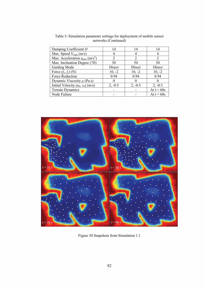
82
Table 5: Simulation parameter settings for deployment of mobile sensor networks (Continued)
Damping Coefficient D 14 14 14 Max. Speed Vmax (m/s) 4 4 4 Max. Acceleration amax (m/s2) 2 2 2 Max. Inclination Degree (°D) 50 50 50 Guiding Mode Direct Direct Direct Force (fx, fy) (N) 10, -2 10, -2 10, -2 Force Reduction 0.94 0.94 0.94 Dynamic Viscosity μ (Pa.s) 0 0 0 Initial Velocity (u0, v0) (m/s) 2, -0.5 2, -0.5 2, -0.5 Terrain Dynamics - - At t = 60s Node Failure - - At t = 60s
Figure 30 Snapshots from Simulation 1.1
t = 10 s t = 30 s
t = 50 s t = 90 s

83
Figure 31 Average robot velocity in Simulation 1.1
Figure 32 Average of robot densities (ρ) versus node density (λ) in the covered area in Simulation 1.1
Node density in Figure 32, on the other hand, is a measure of the number of nodes
per unit area that is covered by the robots. In other words, it is the ratio of total
number of nodes to total area covered by the network. It turns out from Figure 32
that after the network covers the whole area, node density stabilizes at 0.68
nodes/m2. This can also be observed from Figure 34 where coverage versus robot

84
number is depicted. The final value of the robot number is 87 and coverage is 128
m2. The steady increase of coverage with respect to the number of nodes shows
that the self-deployment method is scalable with the network size and hence with
the environment size. Transient drops in node number at around t = 23s, 36s, and
50s are due to those nodes that escape from the environment during the initial
stages of their deployment. It can be seen from the guiding parameters of this
simulation in Table 5 that each robot is assigned a body force heading into the
environment. However, this force quickly dies out due to force reduction (FR)
parameter being 0.94. Remembering from Table 4 that the body force with respect
to time in direct mode is given by f (t)=(FR)t/∆t (fx, fy). For example, this initial
body force becomes (0.02, -0.004) at t = 5s. In this simulation, injection of new
nodes was manually stopped at time t = 60s and the entrance of the environment
was virtually closed afterwards so that no robot can get out of the terrain. The
resulting coverage graph shows that the area covered by the network starts
saturating at around t = 40s. In the final configuration, the area covered by the
network is illustrated in Figure 35. It can be seen that the uniformity of distribution
is degraded around obstacles. This is because the obstacles constrain the motion of
robots. In uniformly covered areas, the coverage circles of nodes almost
tangentially intersect each other. This is because of a special selection of
deployment radius Rd (1.6m) twice the sensing radius Rs.

85
Figure 33 Average separation among neighboring robots with its standard deviation
Figure 34 Coverage versus robot number in Simulation 1.1

86
Figure 35 Coverage circles of the nodes in Simulation 1.1
5.2.3 Simulation 1.2: Adjusting Node Density using Deployment Radius
As it was mentioned in the previous chapter, we can play with the deployment
radius parameter to obtain a more densely or sparsely deployed network. By
deploying more robots, redundancy in the network can be improved as the
probability of a point in the terrain being covered by at least one sensor increases.
Conversely, increasing the deployment radius may be necessary due to insufficient
number of robots in expense of leaving uncovered areas between robots. In this
case, a hardware solution would be to improve the sensing range of the robots.
In this simulation, the radius of deployment is reduced to 1.4m as shown in the
third column of Table 5 without changing the other parameters. The resulting
coverage graph is shown in Figure 36, where deployment is apparently denser.
Also, some of the areas, e.g. the upper left corner, which could not be covered
previously, are now better covered. In qualitative terms, Figure 37 tells that the
final value of robot number is 134 while coverage is 158 m2. This means that there

87
are 0.85 nodes per m2 as can also be seen from Figure 38. Therefore, when
compared with the previous case, coverage increases from 128 m2 to 158 m2 in
expense of deploying 137 sensor nodes.
Figure 36 Coverage when deployment radius decreased to 1.4m in Simulation 1.2

88
Figure 37 Coverage versus robot number in Simulation 1.2
Figure 38 Average of robot densities (ρ) versus node density (λ) in the covered area in Simulation 1.2
5.2.4 Simulation 1.3: Dynamical Changes in Environment and Network
In order to demonstrate the fault tolerance and adaptivity of the self deployment
algorithm to node failures and terrains dynamics, we analyze a scenario in which

89
an obstacle in the terrain is destroyed along with some surrounding nodes. We
consider the same simulation in 1 with the destruction of the island-like obstacle
inside the terrain and surrounding 3 nodes at time t = 60s. Figure 39 shows the
snapshots of the instant of this dynamical change and the ensuing recovery of the
destructed region. When the middle obstacle is destroyed with 3 surrounding
nodes at t = 60, a large uncovered area emerges. Since this spare area is a region of
low pressure for the surrounding nodes, the network adapts to this dynamical event
and starts flowing into this gap. Eventually, the system compensates for the failure
of nodes and recovers the whole environment as can be seen from Figure 40 and
Figure 41.
Figure 39 Snapshots from Simulation 1.3: Obstacle in the middle is destroyed at t = 60s
t = 60 s t = 60+ s
t = 65 s t = 90 s

90
Figure 40 Coverage after the middle obstacle is destroyed
Figure 41 Effect of the dynamical environment change and node failure on coverage

91
5.3 Navigation and Path Following
As briefly mentioned in the previous chapter, there are several flow parameters
summarized in Table 3 that effect the behavior of a multi-robot system both in the
global and local scales and provide some desirable characteristics in terms of
navigation capabilities. For example, a nonzero viscosity results in the generation
of a boundary layer around obstacles such that robots moving along obstacle
surfaces slow down and the possibility of colliding with them is reduced. Another
aspect of viscosity is that it provides a coherence mechanism among robots such
that a local perturbation on the system propagates to the rest through shear and
normal stresses among robots.
The most important mechanism of global control in the fluid dynamics framework
is the concept of body force. It is such a force that directly acts on each individual
and can guide the motion towards a desired direction. This parameter is utilized in
the following simulations to demonstrate its potential use in navigation tasks.
5.3.1 Simulation 2.1: Single Waypoint Navigation
In this simulation, flow of a number of robots in an outdoor terrain toward a fixed
waypoint beyond obstacles is demonstrated. In Figure 42, a typical outdoor
environment is shown with the indications of the regions where the robots enter
and leave the environment. In order to guide robots through this terrain, the body
force parameter f in (34) is utilized. It is seen that the area between the start and
destination regions is obstructed by hills upon which robots cannot climb.
Therefore, the system has to flow around these obstacles.
The second column in Table 6 summarizes the flow parameters used in this
simulation. Note that the guiding mode is selected as “Route” so that the body
force applied to each robot points to the destination region which is like a
waypoint for the robots to reach. In this simulation, it is assumed that the robots
know the relative location of this waypoint. This capability can be provided to the
robots by equipping each of them with a GPS (Global Positioning System)
receiver. Therefore, we implemented a decentralized waypoint navigation

92
algorithm given in Listing 3 as the collective control layer of the fluid dynamics
framework.
Figure 42 An outdoor simulation environment for navigation tasks
Table 6 Simulation parameter settings for navigation in outdoor environments
Parameter Sim.2.1 Sim. 2.2 Flow Mode Inviscid Inviscid Deployment Mode Adaptive Adaptive Gas/Liquid Gas Gas Initial Density λ 2 1.2 Simulation Time (s) 40 40 Communication Radius Rc (m) 3.2 3.2 Deployment Radius Rd (m) 1.6 1.6 Sensing Radius Rs (m) 1.2 1.2 Pressure Constant R (J/mol.K) 1 0.5 Time Step ∆t (m) 0.05 0.05 Normal Avoidance Factor A 2 2 Ambient Temperature Tamb (K) 1 1 Max. Nodal Spacing C 1 1 Damping Coefficient D ∞ ∞ Max. Speed Vmax (m/s) 3 3 Max. Acceleration amax (m/s2) 3 3 Max. Inclination Degree (°D) 50 50 Guiding Mode Route Route Waypoints (x, y) (m) (49, 17) (16,16), (39,7), (49, 17) Force Magnitude (N) 6 6 Dynamic Viscosity μ (Pa.s) 0 0 Initial Velocity (u0, v0) (m/s) 0, 0 0, 0

93
The algorithm in Listing 3 basically calculates the body force vector of a robot
according to the relative position of the target waypoint such that the body force
takes a direction pointing toward the coordinate of the waypoint given as (xW, yW)
= (49, 17) m in the simulation parameter setting. While not available in this
simulation, in the following simulations there are multiple waypoints that are to be
navigated progressively. The 4th step of the algorithm tells that when a robot
approaches to a waypoint closer than the communication range, it switches the
body force to the next waypoint so that it can smoothly navigate through all the
waypoints up to the destination.
Listing 3 Pseudocode for decentralized waypoint navigation algorithm of a robot
1 Get the force magnitude parameter fM and sensing radius Rc 2 Get the next waypoint coordinate (xW, yW) 3 Calculate relative distance to the waypoint d = |(xi, yi) – (xW, yW)| 4 If d > Rs/2 5 Calculate relative bearing of the waypoint θ = arctan((yW – yi)/(xW – xi)) 6 Calculate the body force as fi = (fx, fy) = fM (1 – Rc/d)(cosθ, sinθ) 7 Else 8 Go to step 2
Application of this algorithm along with the fluid model parameterized in the
second column of Table 6 produces the result shown in Figure 43 where snapshots
from six instants of the simulation are given. There are totally 50 robots that enter
the environment from the lower left edge and navigate thorough obstacles to the
exit at the upper right edge. It can be seen that the robots separate into two when
they come across with the first hill and then rejoin to pass through a narrow
passage between two other hills.

94
Figure 43 Snapshots from Simulation 2.1
5.3.2 Simulation 2.2: Path Following Using Multiple Waypoints
In the previous simulation, there was a single waypoint behind obstacles around
which the robots had to flow. To some extent, the robots were free to move around
while avoiding obstacles. In some applications, however, the path of the robot herd
may be thoroughly predetermined by multiple waypoints along a track as in Figure
44 for instance. In such a case, the flow of the robots needs to be constrained in a
thin path so that they do node disperse undesirably. In order to funnel down the
robots along such a path, the system might either be modeled as a liquid as
mentioned in Chapter 4 or as a gas with a low specific gas constant R. Using a low
R value, the robots do not repel each other considerably and they can be
concentrated over a track and directed along the route under a suitable body force.
In this simulation, we adopt to use a lower R value as can be seen in the third
column of Table 6 where it is taken as 0.5. Again using the algorithm in Listing 3,
the result in Figure 45 is obtained. In contrast to the previous simulation, the
robots do not disperse over the environment and can maintain a sequence along a
trajectory that connects the waypoints.
t = 2s t = 8s
t = 13s t = 18s
t = 23s t = 31s

95
Figure 44 Waypoint locations in Simulation 2.2
Figure 45 Path following through multiple waypoints in Simulation 2.2
The plot in Figure 46 shows the average robot velocity with respect to time. The
mean velocity level is below 3m/s due to the velocity limitation given in the
second column of Table 6 with Vmax parameter. It can be noted that the robots
t = 3s t = 9s
t = 14s t = 20s
t = 27s t = 35s
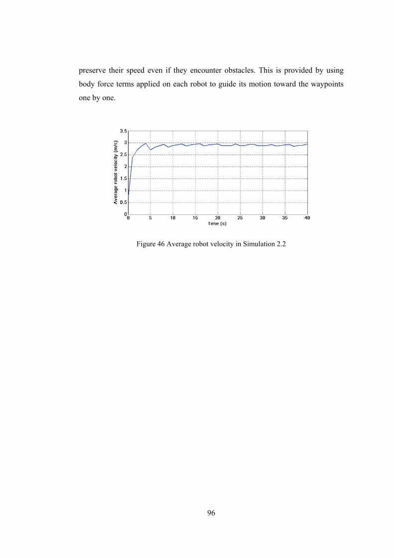
96
preserve their speed even if they encounter obstacles. This is provided by using
body force terms applied on each robot to guide its motion toward the waypoints
one by one.
Figure 46 Average robot velocity in Simulation 2.2
97
CHAPTER 6
CONCLUSION AND FUTURE WORK
In this thesis, a fluid dynamics inspired framework for control of large-scale multi-
robot systems is presented. The framework defines two basic architectural levels
of control called as fluid dynamics layer in the lower level and collective control
layer in the upper level. In the lower layer, the fluid dynamics model controls
multi-robot system behaviors based on Smoothed Particle Hydrodynamics (SPH).
The model provides a set of parameters through which the upper layer controls
both local interactions among robots and their global behavior. Therefore, the two-
layer architecture provides the control of the fluid dynamics based model for
collective multi-robot systems. The novelty of this approach is that it proposes a
dynamically controllable model; in contrast to the existing physics based
methodologies that rely on static and predetermined artificial physics properties in
their models. Also the proposed approach is considered a precursor for the
development of a fully explored fluid dynamics model for large-scale multi-robot
systems. While we agree with the notion of emergent collective behavior
emanating from local interactions of robots in a large-scale multi-robot system, we
also believe in the benefit of being able to control these interactions and the
collective behavior via a well defined framework. In this respect, we believe that
the proposed novel method will extend the idea of emergent behavior in collective
robotics.
The theory of fluid dynamics and the associated numerical analyses techniques
like SPH are mature and provide a profound background to its exploitation in our
framework. Hence, it is important to derive adequate analogies between fluid
physics and mobile robots. Nonetheless, it may not always be possible to map
concepts from one side to the other. In this case, methodologies that are already
available in the robotics literature and suitable for such possible gaps may be
equally used.

98
In the experimental validation of the proposed method, two common problems in
multi-robot systems, deployment control and navigation, were addressed. It was
shown that using the parameters of the framework, different global and local
behaviors can emerge from local interactions of robots. While self-deployment of
mobile sensor networks was due to the dispersion nature of a gas-like system,
navigation and path following capabilities of robots in unstructured environments
were facilitated by guiding body forces and by the inherent reactivity of fluids to
obstacles. The foremost extension to the demonstration of the capabilities of the
fluid dynamics model would be to deal with the formation control problem. It was
shown in the deployment simulations that steady state configuration of a gas-like
robot network exhibits an intrinsic hexagonal lattice formation. We think that this
is a result of the circular support domain and the associated smoothing function.
We strongly anticipate that by using different shapes for support domains and
smoothing functions, different formation shapes can be obtained.
Although the present discussion hopefully reveals the potential applicability of the
proposed method to general collective robotics problems, there remain various
aspects for improvements both in the fluid dynamics framework and in the
experimental setup used to test the developed algorithms. First, an in depth
sensitivity analysis should be carried out on the individual effect of each flow
parameter involved in the governing equations and on their combined utilization
for truly understanding the overall control capabilities of the fluid dynamics
model. Besides, optimal control of these parameters by the high level control layer
toward performing a robotic task in the best way is a challenging issue that needs a
large scope consideration. On the other side, the design of the high level control
layer of the framework for various applications would demonstrate possible
common features that could be used as guidelines to generalize the structure of the
layer and ease the process of redesigning it for different applications. Similarly, in
order to be able to make predictions on the macroscopic behavior of the resulting
design, statistical analyses on large sets of experimental data may be carried out.
We envisage that such an analysis would reveal a predominant deterministic

99
component in the macroscopic model of a fluid-like multi-robot system whose
constituents have definite, physics based mathematical descriptions.
As for further experimentation of the method, the primary improvement would be
to develop a realistic simulator that can simulate embodied agents, sensing
uncertainties, communication aspects, more complex environment features, and
various real robot dynamics. Also, different new techniques in computational fluid
dynamics and Smoothed Particle Hydrodynamics may be incorporated into the
simulator to benefit from the improvements in those areas.
Finally, the ultimate goal of any future work is to realize the developed
methodology first in the laboratory and then in the real world. We truly hope to see
a robotic technology contributed by the work in this thesis to appear eventually at
some time in the future, saving lives in disaster areas, providing security for
habitats, or in any way improving the standards of life for human being.

100
REFERENCES
[1] Y. U. Cao, A. S. Fukunaga, A. B. Khang, F. Meng, “Cooperative Mobile Robotics: Antecedents and Directions,” in Proceedings of the 1995 IEEE/RSJ International Conference on Intelligent Robots and Systems, 1995, pp. 226 – 234.
[2] G. Dudek, M. R. M. Jerkin, E. Milios, and D. Wilkes, “A Taxonomy for Multi-Agent Robotics,” Autonomous Robots, Vol. 3(4), pp. 375 – 397, Dec. 1996.
[3] L. E. Parker, “Current State of the Art in Distributed Autonomous Mobile Robotics,” in Proceedings of the Fifth International Symposium on Distributed Autonomous Robotic Systems, 2000, pp. 3 – 12.
[4] T. Arai, E. Pagello, L. E. Parker, “Editorial: Advances in Multi-Robot Systems,” IEEE Transactions on Robotics and Automation, Vol. 18(5), pp. 655 – 661, Oct. 2002.
[5] G. Beni, “From Swarm Intelligence to Swarm Robotics,” Swarm Robotics: State-of-the-Art Survey, Lecture Notes in Computer Science 3342, Springer-Verlag, pp. 1 – 9, 2005.
[6] E. Şahin, “Swarm Robotics: From Sources of Inspiration to Domains of Application,” Swarm Robotics: State-of-the-Art Survey, Lecture Notes in Computer Science 3342, Springer-Verlag, pp. 10 – 20, 2005.
[7] T. Balch, R. C. Arkin, “Communication in Reactive Multiagent Robotic Systems,” Autonomous Robots, Vol. 1(1), pp. 27 – 52, 1994.
[8] I. F. Akyildiz, W. Su, Y. Sankarasubramaniam, E. Cayirci, “A Survey on Sensor Networks,” IEEE Communications Magazine, pp. 102 – 114, Aug. 2002.
[9] C.-Y. Chong, S. P. Kumar, “Sensor Networks: Evolution, Opportunities, and Challenges,” Proceedings of the IEEE, Vol. 91(8), pp. 1247 – 1256, Aug. 2003.
[10] J. T. Feddema, C. Lewis, D. A. Schoenwald, “Decentralized Control of Cooperative Robotic Vehicles: Theory and Application,” IEEE Transactions on Robotics and Automation, Vol. 18(5), pp. 852– 864, Oct. 2002.
[11] D. Fox, J. Ko, K. Konolige, B. Limketkai, D. Schulz, B. Stewart, “Distributed Multirobot Exploration and Mapping,” Proceeding of the IEEE, Vol. 94(7), pp. 1325 – 1339, Jul. 2006.

101
[12] W. Burgard, M. Moors, D. Fox, R. Simmons, S. Thrun, “Collaborative Multi-Robot Exploration,” in Proceedings of the IEEE International Conference on Robotics and Automation, 2000, pp. 476 – 481.
[13] A. Howard, L. E. Parker, G. S. Sukhatme, “Experiments with a Large Heterogeneous Mobile Robot Team: Exploration, Mapping, Deployment and Detection,” International Journal of Robotics Research, Vol. 25(5-6), pp. 431 – 447, May – June, 2006.
[14] K. Konolige, D. Fox, C. Ortiz, A. Agno, M. Eriksen, B. Limketkai, J. Ko, B. Morisset, D. Schulz, B. Stewart, R. Vincent, “Centibots: Very large scale distributed robotic teams,” in Proceedings of the International Symposium on Experimental Robotics, 2004.
[15] J. Ota, T. Arai, “Transfer control of a large object by a group of mobile robots,” Robotics and Autonomous Systems, Vol. 28(4), pp. 271 – 280, 1999.
[16] R. Alami, S. Fleury, M. Herrb, F. Ingrand, F. Robert, “Multi-Robot Cooperation in the MARTHA Project,” IEEE Robotics and Automation Magazine, Vol. 5(1), pp. 36 – 47, Mar. 1998.
[17] A. Martinoli, K. Easton, W. Agassounon, “Modeling Swarm Robotic Systems: A Case Study in Collaborative Distributed Manipulation,” The International Journal of Robotics Research, Vol. 23(4-5), pp. 415 – 436, 2004.
[18] P. Rbyski, N. P. Papanikolopoulos, S. A. Stoeter, D. G. Krantz, K. B. Yesin, M. Gini, R. Voyles, D. F. Hougen, B. Nelson, M. D. Erickson, “Enlisting Rangers and Scouts for Reconnaissance and Surveillance,” IEEE Robotics and Automation Magazine, Vol. 7(4), pp. 14 – 24, Dec. 2000.
[19] V. Kumar, D. Rus, S. Singh, “Robot and Sensor Networks for First Responders,” IEEE Pervasive Computing, Vol. 3(4), pp. 24 – 33, Oct. – Dec. 2004.
[20] I. Nourbakhsh, K. Sycara, M. Koes, M. Yong, M. Lewis, S. Burion, “Human-Robot Teaming for Search and Rescue,” IEEE Pervasive Computing, Vol. 4(1), pp. 72 – 78, Jan. 2005.
[21] P. Kundu and I. M. Cohen, Fluid Mechanics, Academic Press, Elsevier Science, 2002.
[22] K. Lerman, A. Martinoli, A. Galstyan, “A Review of Probabilistic Macroscopic Models for Swarm Robotic Systems,” Swarm Robotics: State-of-the-art Survey, Lecture Notes in Computer Science 3342, E. Şahin W. M. Spears, Eds., Berlin Heidelberg: Springer-Verlag, pp. 143 – 152, 2005.

102
[23] M. J. Mataric, “Situated Robotics,” Encyclopedia of Cognitive Science, Nature Publishers Group, Macmillian Reference Ltd., 2002.
[24] L. Iocchi, D. Nardi, M. Salerno, “Reactivity and Deliberation: A Survey on Multi-Robot Systems,” in Balancing Reactivity and Deliberation in Multi-Agent Systems, Lecture Notes in Computer Science 2103, E. P. M. Hannebauer, J. Wendler, Eds., Springer, pp. 9 – 34, 2001.
[25] A. Farinelli, L. Iocchi, D. Nardi, “Multi-Robot Systems: A Classification Focused on Coordination,” IEEE Transactions on Systems, Man, and Cybernetics, Vol. 34(5), pp. 2015 – 2028, Oct. 2004.
[26] R. A. Brooks, “A Robust Layered Control System for a Mobile Robot,” IEEE Journal on Robotics and Automation, Vol. RA-2(1), pp. 14 – 23, March 1986.
[27] L. E. Parker, “Designing Control Laws for Cooperative Agent Teams,” in Proceedings of the IEEE International Conference on Robotics and Automation, 1993, pp. 582 – 587.
[28] M. Mataric, “Interaction and Intelligent Behavior,” PhD Thesis, MIT, 1994.
[29] L. E. Parker, “On the Design of Behavior-Based Multi-Robot Teams,” Advanced Robotics, Vol. 10(6), pp. 547 – 578, 1996.
[30] L. E. Parker, “ALLIANCE: An Architecture for Fault Tolerant Multirobot Cooperation,” IEEE Transactions on Robotics and Automation, Vol. 14(2), pp. 220 – 240, Apr. 1998.
[31] T. Balch, R. C. Arkin, “Behavior-Based Formation Control for Multirobot Teams,” IEEE Transactions on Robotics and Automation, Vol. 14(6), pp. 926 – 939, Dec. 1998.
[32] O. Khatib, “Real-time obstacle avoidance for manipulators and mobile robots,” in Proceedings of the IEEE International Conference on Robotics and Automation, 1985, pp. 500 – 505.
[33] J. Borenstein, Y. Yoren, “Real-Time Obstacle Avoidance for Fast Mobile Robots,” IEEE Transactions on Systems, Man, and Cybernetics, Vol. 19(5), pp. 1179 – 1187, Sep. – Oct. 1989.
[34] Y. K. Hwang, N. Ahuja, “A Potential Field Approach to Path Planning,” IEEE Transactions on Robotics and Automation, Vol. 8(1), pp. 23 – 32, Feb. 1992.
[35] S. S. Ge, Y. J. Cui, “New Potential Functions for Mobile Robot Path Planning,” IEEE Transactions on Robotics and Automation, Vol. 16(5), pp. 615 – 620, Oct. 2000.

103
[36] E. Rimon, D. E. Koditschek, “Exact Robot Navigation Using Artificial Potential Functions,” IEEE Transactions on Robotics and Automation, Vol. 8(5), pp. 501 – 518, Oct. 1992.
[37] A. Howard, M. Mataric, G. S. Sukhatme, “Mobile Sensor Network Deployment using Potential Fields: A Distributed, Scalable Solution to the Area Coverage Problem,” in Proceedings of the Sixth International Symposium on Distributed Autonomous Robotics Systems, 2002, pp.299 – 308.
[38] D. H. Kim, H. Wang, S. Shin, “Decentralized Control of Autonomous Swarm Systems Using Artificial Potential Functions: Analytical Design Guidelines,” Journal of Intelligent Robots and Systems, Vol. 45(4), pp. 369–394, 2006.
[39] T. Balch, M. Hybinette, “Social Potentials for Scalable Multi-Robot Formations,” in Proceedings of the IEEE International Conference on Robotics and Automation, 2000, pp. 73 – 80.
[40] Y. Koren, J. Borenstein, “Potential Field Methods and Their Inherent Limitations for Mobile Robot Navigation,” in Proceedings of the IEEE International Conference on Robotics and Automation, 1991, pp. 1398 – 1404.
[41] J. Ren, K. A. McIsaac, R. V. Patel, “Modified Newton’s Method Applied to Potential Field-Based Navigation for Mobile Robots,” IEEE Transactions on Robotics and Automation, Vol. 22(2), pp. 384 – 391, Apr. 2006.
[42] J. Decuyper, D. Keymeulen, “A Reactive Robot Navigation System Based on a Fluid Dynamics Metaphor,” Parallel Problem Solving from Nature, Lecture Notes in Computer Science, Springer-Verlag, pp. 348 – 355, 1990.
[43] D. Keymeulen, J. Decuyper, “The Fluid Dynamics Applied to Mobile Robot Motion: the Stream Field Method,” in Proceedings of the IEEE International Conference on Robotics and Automation, 1994, pp. 378 – 385.
[44] J.-O. Kim, P. K. Khosla, “Real-Time Obstacle Avoidance Using Harmonic Potential Functions,” IEEE Transactions on Robotics and Automation, Vol. 8(3), pp. 338 – 349, Jun. 1992.
[45] C. Louste, A. Liegeois, “Near Optimal Robust Path Planning for Mobile Robots: the Viscous Fluid Method with Friction,” Journal of Intelligent and Robotic Systems, Vol. 27, pp. 99 – 112, 2000.
[46] D. Zarzhitsky, D. Spears, D. Thayer, W. Spears, “Agent-Based Chemical Plume Tracing Using Fluid Dynamics,” Formal Approaches to Agent Based

104
Systems, Lecture Notes in Computer Science 3228, Springer-Verlag, pp. 146 – 160, 2004.
[47] D. Zarzhitsky, D. F. Spears, W. M. Spears, “Swarms for Chemical Plume Tracing,” in Proceedings of the IEEE Swarm Intelligence Symposium, 2005, pp. 249 – 256.
[48] W. M. Spears, D. F. Gordon, “Using Artificial Physics to Control Agents,” in Proceedings of the International Conference on Information, Intelligence, and Systems, 1999, pp. 281 – 288.
[49] W. Kerr, D. Spears, W. Spears, D. Thayer, “Two Formal Gas Models for Multi-Agent Sweeping and Obstacle Avoidance,” Formal Approaches to Agent Based Systems, Lecture Notes in Computer Science 3228, Springer-Verlag, pp. 111 – 130, 2004.
[50] D. Spears, W. Kerr, and W. Spears, “Physics-Based Robot Swarms For Coverage Problems,” International Journal on Intelligent Control and Systems, 11(3), 2006.
[51] J. R. Perkinson, B. Shafai, “A Decentralized Control Algorithm for Scalable Robotic Swarms Based on Meshfree Particle Hydrodynamics,” in Proceedings of the IASTED International Conference on Robotics and Applications, 2005, pp. 102 – 107.
[52] S. Meguerdichian, F. Koushanfar, M. Potkonjak, M. Srivastava, “Coverage Problems in Wireless Ad-hoc Sensor Networks,” in Proceedings of the IEEE Infocom Conference, 2001, pp. 1380-1387.
[53] D. O. Popa, C. Helm, “Robotic Deployment of Sensor Networks Using Potential Fields,” in Proceedings of the 2004 IEEE International Conference on Robotics and Automation, 2004.
[54] N. Heo, P. K. Varshney, “A Distributed Self Spreading Algorithm for Mobile Wireless Sensor Networks,” in Proceedings of IEEE Wireless Communications and Networking Conference, 2003.
[55] N. Heo, P. K. Varshney, “Energy-Efficient Deployment of Intelligent Mobile Sensor Networks,” IEEE Transactions on Systems, Man, and Cybernetics, Vol. 35(1), pp. 78 – 92, Jan. 2005.
[56] Y. Zou, K. Chakrabarty, “Sensor Deployment and Target Localization Based on Virtual Forces,” in Proceedings of IEEE Infocom Conference, vol. 2, 2003.
[57] M. R. Pac, A. M. Erkmen, I. Erkmen, “Towards Fluent Sensor Networks: A Scalable and Robust Self-Deployment Approach,” in Proceedings of the
105
First NASA/ESA Conference on Adaptive Hardware and Systems, 2006, pp. 365 – 372.
[58] M. R. Pac, A. M. Erkmen, I. Erkmen, “Robot Sensor Networks Flow to Deploy,” unrefereed research poster in the Second EURON Summer School on Perception and Sensor Fusion in Mobile Robotics (PSFMR), Fermo, Italy, Sept. 11-16, 2006.
[59] M. R. Pac, A. M. Erkmen, and I. Erkmen, “Scalable Self-Deployment of Mobile Sensor Networks: A Fluid Dynamics Approach,” in Proceedings of the 2006 IEEE/RSJ International Conference on Intelligent Robots and Systems, 2006, pp. 1446 – 1451.
[60] M. R. Pac, A. M. Erkmen, and I. Erkmen, “Control of Robotic Swarm Behaviors Based on Smoothed Particle Hydrodynamics,” to appear in the 2007 IEEE/RSJ International Conference on Intelligent Robots and Systems, 29 Oct. – 2 Nov., 2007.
[61] J. Anderson, Computational Fluid Dynamics, McGraw-Hill, 1995.
[62] G. R. Liu and M. B. Liu, Smoothed Particle Hydrodynamics: A Meshfree Particle Method, World Scientific, 2003.
[63] C. Pozrikidis, Fluid Dynamics: Theory, Computation, and Numerical Simulation, Kluwer Academic Publishers, 2001.

106
APPENDIX A
BOUNDARY CONDITIONS AND SYSTEM CONSTRAINTS
As introduced in part 4.3.5, there are two boundary conditions due to the physics
of fluids for a robot at the surface of an obstacle. First one is the no-slip condition
for viscous flows such that the velocity of a robot diminishes as it comes very
close to a surface. The other is the thermal equilibrium condition at the boundaries.
On the other hand, there are also some constraints inherent to robotic systems.
Two of the most important and general ones are discussed here, namely the
constraints on the locomotion capabilities of and communication connectivity
among robots.
A.1 Obstacle Detection and Avoidance
The capabilities of a mobile robot in detecting obstacles strongly depend on its
sensor modalities such as ultrasonic, infrared or laser sensors. Laser range finders
are the most commonly used sensors in research setups and realizations due to
their accuracy and long range. In unstructured environments, detecting the exact
boundaries of an obstacle is not a trivial task because the terrain features are in
continuum rather than in distinguished states. For example, the environment
shown in Figure 42 is a typical outdoor terrain where the obstacles for a robot can
only be distinguished based on the slope of the ground. That is, the maximum
slope that the robot can move over determines which parts of the environment are
going to be identified as obstacles. In the simulations, we assumed that robots can
measure the slope of the surrounding environment features and detect obstacles as
points in space with respect to the robot itself. A parameter called as ‘Max.
Inclination Degree’ is included in the framework (see Table 4) to determine the
maximum slope the robots can move over.
For fluid-like robots, obstacle avoidance condition can be restated as a requirement
that a robot cannot have a velocity component perpendicular to an obstacle surface

107
if it is very close to the surface. Also, if the fluid model is viscous, then the overall
velocity of the robot ceases at the very vicinity of an obstacle. The figure below
illustrates the variables involved in the formulation of this obstacle avoidance
behavior. Suppose that a robot detects two obstacle points. In order to avoid this, it
calculates the two components of its velocity with respect to the surface that can
be defined with these two points. If the robot happens to detect only one point, it
can assume a surface passing through this point and perpendicular to the line
between this point and the robot.
Figure 47 Illustration for the mathematical formulation of obstacle avoidance
Using some geometry, the parallel component of the robot velocity with respect to
the two obstacle points can be derived as in (42). As a measure of the robot’s
proximity to the surface, a factor k is defined in (43) such that when the robot
detects an obstacle at Rs –the sensing range– k becomes 1 and it drops to zero as d
goes to zero.
2 2
2 1
2 1
, V
V cos
arctan , arctan
u v
y yvu x x
ϕ θ
ϕ θ θ
⊥= + = = +
= ∠
⎛ ⎞−⎛ ⎞= − = ⎜ ⎟⎜ ⎟ −⎝ ⎠ ⎝ ⎠
V V V V
V (42)

108
1 2 1 2
0 0 2 12 1
1 0 2 1
21
sin cos cos
ss
s
d d RR dk
d R
y x x yx y x xx xd
x x x x
θ θ θ
⎧ ≤⎪ −= ⎨⎪ >⎩
⎧ −− + ≠⎪ −= ⎨
⎪ − =⎩
(43)
Finally, using (44) where Vobs is the corrected velocity of a robot around an
obstacle, the velocity of the robot can be smoothly deviated from a heading toward
the obstacle. In this equation, μ is the viscosity of the multi-robot system and M is
constant that determines the strength of the viscosity effect on the parallel
component of velocity. Thus, the less the viscosity is (i.e. more inviscid), the more
the robot can move in the parallel direction.
(1 ) Mobs k k e μ−= + −V V V (44)
As an extra obstacle avoidance mechanism, we also incorporated an artificial body
force that repels robots in normal direction to the obstacle surfaces. The obstacle
force calculated in (45) is added to the body force term in (34). Here, A is the
normal avoidance factor that adjusts the strength of the normal force.
0 12
0 12
12 1 1 0 0
12 1 1 0 0
, arctan0.001
( sin cos )sin ( cos sin )cos( sin cos )cos ( cos sin )sin
obsy yA
k x xx x y x y
y x y x y
φ φ
θ θ θ θ θ θθ θ θ θ θ θ
⊥ −= ∠ =
+ −
= − + +
= − + + +
f
(45)
A.2 Thermal Equilibrium
Implementation of the boundary condition for temperature also depends on the k
factor as given in (46). Here Tamb is the normal ambient temperature of the robots.
As a robot approaches to a surface, its temperature starts to increase up to 2Tamb,
which is the constant surface temperature.

109
(1 )amb ambT T k T= + − (46)
A.3 Velocity and Acceleration Limitation
The limitations of the robotic system in terms of maximum velocity and
acceleration of robots depend on the physical construction of the robots and can
vary significantly from simple wheeled robots to air vehicles. However, the
constraint on the velocity V and acceleration of a robot can commonly be
described as follows.
2 2 2max
max
2 2 2
max
max
( , , ) V = VV ( , , ) otherwise
V
( , , ) a a
a ( , , ) otherwisea
u v w u v w
u v w
Du Dv Dw Du Dv DwDt Dt Dt Dt Dt Dt
Du Dv DwDt Dt Dt
⎧ + + ≤⎪= ⎨⎪⎩⎧ ⎛ ⎞ ⎛ ⎞ ⎛ ⎞⎪ = + + ≤⎜ ⎟ ⎜ ⎟ ⎜ ⎟⎪ ⎝ ⎠ ⎝ ⎠ ⎝ ⎠= ⎨⎪⎪⎩
V
a
(47)
where Vmax and amax are the maximum values for velocity and acceleration,
respectively.
A.4 Connectivity Constraint
Wireless connectivity among robots is preserved using a damping factor on the
velocity of each robot. The factor applied to the velocity control as follows.
,0 otherwise
Diji i i
i ic
rFF C
R⎧ Ω ≠ ∅ ⎛ ⎞⎪= = −⎨ ⎜ ⎟⎪ ⎝ ⎠⎩
VV (48)
That is, the velocity control calculated from the governing equations is damped if
the set of neighboring robots, the support domain, is not empty. Otherwise, the
robot stops moving until it detects a neighbor. The damping factor is determined
based on the ratio of the average inter-robot distance to the radius of the support
domain. D is the damping factor that scales down the effect of F to adjust the
strength of the constraint. C is a measure of maximum allowed inter-robot spacing
in proportion to Rc.

110
APPENDIX B
PUBLICATIONS OF THE THESIS
B.1 Scalable Self-Deployment of Mobile Sensor Networks
Publication: In Proceedings of the 2006 IEEE/RSJ International Conference on
Intelligent Robots and Systems (IROS), Beijing, China, Oct. 9-15, 2006, pp. 1446
– 1451.
Title: Scalable Self-Deployment of Mobile Sensor Networks: A Fluid Dynamics
Approach
Authors: Muhammed R. Pac, Aydan M. Erkmen, Ismet Erkmen.
Abstract: We propose in this paper a novel approach inspired by fluid dynamics
as a distributed and scalable solution to the deployment problem of mobile sensor
networks in unknown environments. Our approach is based on the physical
principles of fluids through which we model each sensor/robot node as a fluid
element and the sensor network as a fluid body to which we adapt the principles of
fluid flow. Originating from local neighborhood interactions, governing flow
equations of a sensor node is formalized. Mimicking the diffusive and self-
spreading behavior of compressible fluids in a mobile sensor network, we achieve
the desirable properties of effective coverage, scalability, and distributed self-
deployment. Simulation results exhibit the diffusive and self-spreading
characteristics of the nodes producing an emergent collective behavior of the
network towards better coverability. An adaptive deployment scheme is also
devised for urban disaster environments where the number of nodes to be deployed
may not be determined a priori. Simulation of this scenario shows that our
approach is scalable and can guarantee a desired level of service quality without
any prior information about the environment.
111
B.1.1 Introduction
Mobile sensor networks have recently emerged as a new technology integrating
various fields such as sensor fusion, wireless ad-hoc communication, and
distributed robotics. The basic idea of mobile sensor networking is to deploy smart
sensor nodes ‘en masse’ within an environment for surveillance, data mining, and
search. Being the building block of a distributed sensor network, capabilities of an
individual node in terms of sensing, onboard computation, networked wireless
communication, and locomotion enable the whole network to execute numerous
distributed tasks through multilevel collaboration. Although initially the main
drive of research on sensor networks was military [1], civil applications have also
found new emphases by technological improvements. Recently, availability of
inexpensive smart micro-sensors embedded in mobile platforms opened the way to
new robot/sensor network applications such as in disaster intervention and
emergency search-and-rescue [2].
One of the most fundamental concepts in sensor networking is coverage. It is the
quality-of-service that a network can provide [3] and may be defined by the
percentage of the surveillance area that is sensed through sensor nodes. Coverage
is strongly dependent on the deployment of the sensor network over the
environment. Therefore, terrain and task coverage for efficient surveillance and
mission realization stemming from effective deployment are critical control
problems to be dealt with.
The challenges posed by large-scale mobile sensor networks in unknown,
unstructured, and hostile environments necessitate the utilization of distributed
self-deployment schemes, in which deployment is an emergent behavior of the
local coordination among sensor nodes. In this paper, we develop a novel approach
inspired by fluid dynamics as a distributed and scalable solution to the deployment
problem. Our approach is based on the governing physical principles of fluids
where we model the sensor network as a fluid body and each sensor/robot node as
a fluid element. Our motivation is to mimic the diffusive and self-spreading
behavior of compressible fluids, e.g. gases, in a mobile sensor network so as to

112
achieve the desirable properties of effective coverage, scalability, and distributed
self-deployment within an emergent collective behavior. We envisage one of the
potential applications of our approach to be in the fast emergency response for
early stage search-and-rescue operations in which the assistance of mobile sensor
networks are life-critical in unknown, hazardous, and highly unstructured
environments of disaster areas.
B.1.2 Related Works and Motivation
One of the earliest studies on the subject proposes an incremental deployment
algorithm [4] in which each node is deployed one at a time depending on the
information provided by previously deployed nodes to maximize coverage. In this
approach, the computational capacity required for determining the next
deployment location increases proportionally with the number of deployed nodes.
Therefore, serious scalability limitations exist for large-scale networks due to the
centralized nature of this approach. Another algorithm [5] introduces the concept
of force inspired by the equilibrium of molecules. Utilizing the mobility of the
sensor nodes, the algorithm aims at improving the topology of the network that has
random initial deployment. Although there is no explicit reference to the
assumptions about the environment, the target application area is envisaged to be
air dropped sensor networks in rural fields. Indoor environments and obstacle
avoidance are not addressed in this work.
The study of Howard, Mataric, and Sukhatme in [6] provides a solution to the
problem of deploying a mobile sensor network in unknown dynamic
environments. They describe a potential-field-based approach to deployment, in
which nodes are treated as virtual particles, subject to virtual forces. These forces
repel nodes from each other and from obstacles, and ensure that from an initial
compact configuration, nodes will spread out to maximize the coverage area of the
network. Similarly, the virtual force algorithm of [7] and the virtual spring force
algorithm of [8] use both repulsive and attractive force components to maximize
coverage and uniformity for a given number of sensors. Other potential field

113
approaches analyze connectivity and redundancy constraints [9] or include robot
team concepts in sensor networking [10].
A common feature of the existing distributed algorithms mentioned so far is that
deployment is conceived as a coverage process that maneuvers the sensor nodes
from an initial random/compact configuration to a suboptimal configuration in
which a static equilibrium is attained and coverage requirements are met. Although
these approaches assume an unknown sensing environment, all of them implicitly
assume prior information about the surveillance area’s physical range. Thus, each
of them considers the deployment of a predetermined and fixed number of sensor
nodes so that the network reaches the static equilibrium when the nodes disperse
sufficiently over the environment and a certain level of area coverage is achieved.
However, if the size of the surveillance environment is not known a priori –which
is the probable case in urban disaster scenarios due to fractal dimension of the
irregular terrain–, these algorithms can only provide coverage to the size extent of
the area that is previously fixed by the number of nodes to be deployed. Thus, a
certain quality of service could not be guaranteed without prior knowledge of
coverage area size.
We examine in this paper the deployment problem in truly unknown environments
whose physical range is not known and hence the number of sensor nodes to be
deployed cannot be determined a priori. The main contribution of our work is to
present a formalism for modeling a sensor network itself as a fluid penetrating and
diffusing into a terrain with fractional dimensions.
To our knowledge, mobile sensor networks or robot teams have not been modeled
as fluids by the physical principles of fluid dynamics. A fluid dynamics approach
for multi-robot chemical plume tracing is addressed in [11] where flow variables
of a ‘real’ fluid are measured by a computational sensor grid and the flow direction
is estimated for backward tracing. Another work [12] proposes two gas models,
one of which uses a virtual force approach and the other uses a kinetic approach.
The former approach is very similar to the previously discussed virtual force
approaches [5], 7] and is not based on the real physics of gases. The latter, on the

114
other hand, uses the kinetic theory of gases to model obstacle avoidance and deals
with virtual couette walls to introduce kinetic energy into the system.
B.1.3 Model Preliminaries
Assumptions: First, we assume that sensing coverage area of each sensor/robot
node is determined by its sensing range taken as circular in shape with a certain
radius denoted by Rs. Similarly, the communication coverage is the area bounded
by another circle of radius Rc. Nodal coverage in both of these ranges are assumed
to be deterministic. An important assumption is that a sensor node can determine
the relative position of its neighbors that lie within its communication range. This
may be by virtue of utilizing a scanning laser range-finder or communicating the
coordinate information obtained from a global positioning system (GPS). An
exclusive assumption of our approach is that at any time a sensor node knows its
velocity vector with respect to a local or global reference. Also, it can be informed
of the velocities of its neighbors through communication and if needed convert
them into its own reference frame.
Governing Equations of Fluid Dynamics: Fluid dynamics is based on the
mathematical statements of three fundamental physical principles, namely
conservation of mass, Newton’s second law, and conservation of energy. The
governing equations of fluid flow are derived by applying these principles to a
suitable flow model. One of the flow models that we adopt in our approach
considers the fluid body as a collection of flowing infinitesimal fluid elements. It
is called the nonconservation form flow model. In the development of our
approach, we model a mobile sensor network as an inviscid compressible fluid
composed of individual fluid elements, i.e. sensor nodes. The governing equations
for the flow of such a fluid in two dimensions are expressed as in (1).
:
:
x
y
Du px momentum fDt xDv py momentum fDt y
ρ ρ
ρ ρ
∂= − +∂∂= − +∂
(1)

115
Equation (1) is called the Euler Equations in which ρ is fluid density, D/Dt is the
substantial derivative, p is fluid pressure, fx and fy are body force components per
unit mass in x and y directions, and finally u and v are the velocity components of
an infinitesimal fluid element in the respective directions. This equation can be
rearranged in a convenient form as in (2)
,
,
1
1
t t t tt t ti i i ii i i xt
it t t t
t t ti i i ii i i yt
i
u u u pu v ft x y x
v v v pu v ft x y y
ρ
ρ
⎛ ⎞⎜ ⎟⎜ ⎟⎝ ⎠⎛ ⎞⎜ ⎟⎜ ⎟⎝ ⎠
∂ ∂ ∂ ∂= − + + +∂ ∂ ∂ ∂
∂ ∂ ∂ ∂= − + + +∂ ∂ ∂ ∂
(2)
by using the open form of the substantial derivative terms and time derivatives
isolated on the left-hand side and spatial derivatives on the right-hand side of the
equation. In (2), subscript i and superscript t indicate that the flow variables u, v, ρ,
p, and f belong to the ith element of the fluid at time t. For the details of fluid
dynamics concepts discussed in this paper and derivations of governing equations,
please refer to [13].
B.1.4 A Fluid Dynamics Solution to the Deployment Problem
A distributed deployment scheme, which is necessarily sensor node oriented, has
to originate from the interactions of nodes with their neighbors and surrounding
environment. It is the interactions of a fluid element with its surrounding and the
physical principles governing these interactions that shape our fluid dynamics
based deployment strategy. With appropriate adaptations of fluid concepts to
mobile sensor networks, we aim at providing a suitable formalism for our
distributed deployment approach.
Before the development of our approach, it would be beneficial to explicitly set the
analogy that we found between a flowing fluid and a mobile sensor network as in
Table B.1.1.

116
Table B.1.1 Analogy between a Fluid and a Mobile Sensor Network
Fluid Mobile Sensor Network Fluid body Sensor network Fluid element Sensor node Interactions among adjacent fluid elements
Interactions among neighboring sensor nodes
Fluid flow Network deployment Physical principles of flow Control algorithm of deployment
Adaptation of Fluid Concepts to Mobile Sensor Networks: In accordance with
the aforementioned analogy, we define and reformulate the counterparts of the
flow variables and mathematical expressions appearing in (2) for a mobile sensor
network as follows:
1) Velocity Vector: The velocity vector of a fluid element is directly
analogous to the velocity vector of a sensor node. Thus, the velocity vector of the
ith node (node i) may be denoted by Vit = (ui
t, vit).
2) Local Density: We develop a formalism for the local density denoted by
ρi at a node location as
2
1 1
i
id di i
ij ijj
R R nnr r
ρ∈Ν
= + × = +∑
(3)
Rd is the deployment radius (0< Rd ≤ Rc) of a deployment neighborhood Ni for
node i, defined as the set of neighboring nodes j that fall within this range. ni is the
number of elements in this set and rij is the Euclidean distance between node i and
node j. The variation of local density with respect to average distance between
node i and its neighbors for various values of ni is given in Figure B.1.1. This
definition provides a normalized density value that is proportional to the number
of deployment neighbors and inversely proportional to the average distance
between node i and its neighbors. Therefore, given the same number of elements in

117
set Ni, local density would be higher when nodes are closely located. On the other
hand, if set Ni is empty, density takes the value of 1 to account for node i itself.
3) Pressure: Pressure is the main driving entity in fluid flow. For a perfect
gas, pressure equation is given by
p RTρ= (4)
where R is the specific gas constant and T is the absolute temperature. While we
keep R as a scaling factor in our formulation, we use T for obstacle avoidance
purposes in such a way that nodes that encounter obstacles in their sensing range
raise their temperature, resulting in a repulsive effect on the nodes due to the
higher pressure region generated along the obstacle surfaces as follows
1 (1 )tiT K= + − (5)
where K is defined in (9).
Figure B.1.1 Variation of local density ρi with respect to average inter-nodal distance ijr for various ni number of neighbors
4) Spatial Derivatives of Flow Variables: In equation (2), we have the
partial derivatives of velocity components and pressure with respect to spatial
dimensions x and y. In computational fluid dynamics, these derivatives are found

118
on grid structures using finite difference methods. In sensor networks, however,
the generation of a grid is not practical due to unevenly distributed nature of sensor
nodes. Instead, we formulate a finite difference method based on deployment
neighborhood. We define first-order finite difference equations as in (6) for node i
to approximate the spatial derivatives of flow variables u, v, and p.
( ) ( )
( ) ( )
( ) ( )
1 1cos , sin
1 1cos , sin
1 1cos , sin
t ti i
t ti i
t ti i
t t t tt tj i j ii iij ijt t
ij iji ij j
t t t tt tj i j ii iij ijt t
ij iji ij j
t t t tt tj i j ii iij it t
ij iji ij j
p p p pp px r y rn n
u u u uu ux r y rn n
v v v vv vx r y rn n
θ θ
θ θ
θ θ
∈Ν ∈Ν
∈Ν ∈Ν
∈Ν ∈Ν
− −∂ ∂= =∂ ∂
− −∂ ∂= =∂ ∂
− −∂ ∂= =∂ ∂
∑ ∑
∑ ∑
∑ ∑ j
(6)
We call these as first-order circular difference equations due to the trigonometric
terms multiplying each difference. Here, θij denotes the polar angle of node j with
respect to the reference frame of node i. For the partial derivative with respect to
the x direction, cosine of the relative orientation between node i and its neighbors
places higher emphasis on neighbors along the x direction. Similarly, sine of the
relative orientation places higher emphasis on the neighbors along the y direction
for the partial derivative with respect to y. Differences are also scaled by inter-
nodal distances and averaged over all neighbors within the deployment radius.
Figure B.1.2 (a) and (b) illustrate respectively the variation of the circular weight
terms cosθij/rij and sinθij/rij that determine the emphasis of the flow variable
differences in (6). Note in this figure that θij = tan-1(y/x) and rij = √(x2+y2).
In order to illustrate local interactions within deployment neighborhood, consider a
sensor node, i, with two deployment neighbors, h and k, as in Figure B.1.3.
Arbitrary velocity components are shown for each node within the reference frame
of node i. Also, the relative orientations of the neighboring nodes with respect to
node i are indicated by θih and θik. For the case in Figure B.1.3, (6) yields
positively weighted contributions from node h to the spatial derivatives in both
directions since it is ahead of node i in both directions (cosθih>0, sinθih>0).
Conversely, the contribution of node k to the derivatives in both directions are

119
negatively weighted (cosθik<0, sinθik<0) since it is behind node i in both directions.
Also, the magnitude of the total contribution of node k is more than node h since it
is closer to node i (rik< rih).
Figure B.1.2 Variation of cosθij/rij and sinθij/rij around node i at the origin (0,0)
node-ipi
pknode k
rih
rik
xθih
θik
node-hph uh
vh
ui
vi
uk
vk
Rd
Figure B.1.3 Deployment neighborhood and local interaction parameters
5) Body Forces: In fluid dynamics, a fluid element may be under the effect
of various body forces like gravitational, electric, and magnetic forces. These
forces are incorporated in the governing equations in (1) by fx and fy. Considering a
sensor node as a unit mass element in the network, we modeled fx and fy as force

120
components acting as control entities guiding each node to preferential coverage
regions or target locations. In this way, the network may be directed globally by a
collective network behavior or locally by a clustered network behavior. For
example, a desired patrolling direction determined as a result of the coordination
among sensor nodes may be broadcasted by one of the nodes to impose these body
force components. Alternatively, in a clustered network, each cluster head may
direct its cluster to cover a local isolated target area.
Obtaining Solutions for the Governing Equations: As in computational fluid
dynamics, we obtain computationally the velocity vectors of sensor nodes in the
form of a time-marching solution. For example, take one of the velocity
components u of node i and assume that we know the flow variables at time t.
Then, this velocity component at a differential time interval ∆t later takes the value
given by the Taylor series expansion
( )22
2 2t t
t t t i ii i
tu uu u tt t
+Δ ⎛ ⎞⎛ ⎞⎜ ⎟⎜ ⎟⎜ ⎟ ⎜ ⎟⎝ ⎠ ⎝ ⎠
Δ∂ ∂= + Δ + +∂ ∂
(7)
The velocity component may simply be approximated by the first two terms in (7)
for which all the necessary information is available by (2) through (6). Thus, the
solutions for the velocity components are obtained as
,
,
1
1
t t tt t t t t ti i ii i i i i xt
i
t t tt t t t t ti i ii i i i i yt
i
u u pu u u v f tx y x
v v pv v u v f tx y y
ρ
ρ
+Δ
+Δ
⎛ ⎞⎛ ⎞⎜ ⎟⎜ ⎟⎜ ⎟⎜ ⎟⎝ ⎠⎝ ⎠⎛ ⎞⎛ ⎞⎜ ⎟⎜ ⎟⎜ ⎟⎜ ⎟⎝ ⎠⎝ ⎠
∂ ∂ ∂= + − + + + Δ∂ ∂ ∂
∂ ∂ ∂= + − + + + Δ∂ ∂ ∂
(8)
Limitations, Initial and Physical Boundary Conditions: The solutions obtained
from (8) for the velocity components may exceed the locomotion capabilities of
sensor nodes. Not only velocity, but also its time derivative, i.e. acceleration, may
exhibit a similar behavior. Therefore, we put hard-limiters to the magnitudes of
both velocity and acceleration of sensor nodes in case they exceed respective
thresholds Vth and ath.

121
The time-marching solutions in (8) require the initial values of the velocity
components to be known. In our analyses, we assume zero initial velocities for
every node. Any particular solution is dictated by these initial conditions coupled
with the physical boundary conditions imposed by the environment. The only
boundary condition for inviscid fluid flow is identified to be the requirement that
the velocity vector of a fluid element immediately adjacent to a surface be parallel
to this surface. Adaptation of this condition to the motion of a sensor node is
illustrated in Figure B.1.4 where a sensor node is at a distance d to a surface.
Whenever node i detects a surface (d≤Rs), it changes its velocity through a smooth
deviation from the velocity solution imposed by (8) such that the velocity
eventually becomes parallel to the surface. This is achieved using (9).
'(1 ) , , '
2 's
dK K d d BR d
= + − = = −−
nV V V (9)
where K is the smoothing factor and B is a bias term to determine the minimum
distance that a node is allowed to approach a surface. After applying the boundary
condition, V~ is obtained as the corrected velocity by using an auxiliary vector Vn
normal to the surface tangent.
Figure B.1.4 Illustration of the physical boundary condition
Damping Viscosity for Network Connectivity: In order to preserve the
connectivity of the sensor network, some kind of artificial viscosity that we call
damping viscosity is applied on the nodes so that the residual velocity terms

122
( ),( ti
ti
ti vu=V ) in (8) are scaled by a variable that changes with the average inter-
nodal distance as in (10).
,Dt
ijt t t ii i
c
rF t F C
t R+Δ ⎛ ⎞ ⎛ ⎞
⎜ ⎟ ⎜ ⎟⎜ ⎟⎜ ⎟ ⎝ ⎠⎝ ⎠
∂= + Δ = −∂VV V (10)
Here, F is the damping factor, C is the maximum allowed nodal spacing
proportional to Rc (0<C≤1) and D is an adjustment constant for the level of
damping.
B.1.5 Simulation Results
Numerous simulations have been carried out in various environments to
investigate the performance of our approach in terms of coverability, scalability,
and collectivity of the emergent behavior. Parameter settings of our simulations
are indicated in Table B.1.2 with reference to the related figure number.
In order to illustrate the self-spreading behavior of the sensor nodes under the
connectivity constraint, we deploy a simple network composed of 16 nodes
initially confined to a compact region as shown by square markers in Figure B.1.5
(a) and (b). The final configuration attained after 50 time units for two different
damping viscosity functions F obtained by varying D to impose different
connectivity constraints are shown by the small circles in the same figures. A large
circle around each node indicates its communication range. The variation of local
density and coverage area with respect to time is shown in Figure B.1.6 from
which it is apparent that the initial high density (pressure) results in a fast
deployment during the early stages of the process. This behavior is also exhibited
by sparsely printed points of the streamlines tailing behind the nodes in Figure
B.1.5. Then, the connectivity constraint among the nodes restrains this movement,
driving the network into a static equilibrium with optimal coverage. In Figure
B.1.5 (a), the coverage attained is around 200 square units with each node having
an average of 3.75 neighbors in its communication range. In Figure B.1.5 (b), on
the other hand, maximum coverage is 175 square units with each node having an
average of 10.25 neighbors in its communication range. Therefore, there is a

123
natural tradeoff between coverage and connectivity. By properly adjusting the
parameters of the damping viscosity function in (10), we can achieve a favorable
balance between coverability and connectivity requirements.
Figure B.1.5 Self-spreading of nodes under network connectivity constraint (a) D = 20 (b) D = 10
The obstacle avoidance and directed diffusion capabilities of nodes are illustrated
in Figure B.1.7 where obstacle surfaces are drawn by thick lines. In Figure B.1.7
(a), elapsed time is 50 units and nodes are under the effect of a horizontal body
force. Note fx parameter in the second column of Table B.1.2 assuming a value of
0.5. The result of the same simulation with 150 units of elapsed time, and without
any body force is given in Figure B.1.7 (b). This simulation shows that improved
coverage and fast deployment may be achieved by biasing the deployment of the
network towards a desired direction by using the body force terms available in the
governing equations.
In a bounded environment with obstacles, deployment of a fixed number of sensor
nodes is considered in Figure B.1.8. 24 nodes are released from an initial station
A. After 150 time units, dispersion of nodes throughout the environment almost
ceases. Large circles around the nodes indicate their sensing area at the final
configuration in which the coverage provided is around 250 square units (83% of

124
the maximum that can be obtained from 24 nodes with Rs=2) as shown in Figure
B.1.9. Local density and coverage plots in this figure are obtained for two values
of Rd, 3 and 6, along with the other parameters being the same as indicated in the
3rd column of Table B.1.2.
Table B.1.2 Simulation Settings by Figure Number
Parameter Figure B.1.5 (a,b)
Figure B.1.7 (a,b) Figure B.1.8 Figure B.1.10
Rc 8 4 6 6 Rd 4 2 3, 6 3 Rs 2 1.6 2 1.5 R 0.75 0.75 0.75 1 fx 0 0.5, 0 0 0 fy 0 0 0 0 ∆t 1/20 1/20 1/20 1/20 B 0 0 0.6 0.1 C 1 1 1 1 D 20, 10 4 16 10 Vth 1.5 1.5 1.5 1.5 ath 0.5 0.5 0.5 0.5
Figure B.1.6 Local density and coverage versus time for the simulations in Figure B.1.5

125
When the two plots in Figure B.1.9 are compared, it can be seen that the variation
of coverage with respect to time is similar, whereas transient fluctuations in
coverage and density –due mostly to obstacles– are more significant for the lower
value of the deployment radius. The reason is that when local interactions are
restricted by lower number of neighbors (lower deployment radius), the variation
of spatial derivatives becomes more vulnerable to slight changes in the distribution
of neighbors.
Figure B.1.7 Obstacle avoidance and directed diffusion of nodes (a) t = 50 with a nonzero body force in x direction (b) t = 150 with zero body force
As a final simulation, consider the scenario of deploying a sensor network in a
truly unknown environment whose physical range is not known. Thus, the number
of sensor nodes to be deployed cannot be determined beforehand. For such
scenarios, we switch to our adaptive deployment scheme in which nodes are
injected into the environment one at a time as required. Determining when to
deploy a new node depends on the local node density at the initial deployment
location. When the previously deployed nodes flow into the unobservable depth of
the environment, new successors are placed in the starting locations. This scenario

126
is simulated in a relatively unstructured 3D environment shown in Figure B.1.10.
where the initial deployment location is an opening of the environment indicated
by an arrow at the back edge. Also, there is another opening at the front edge of
the environment indicating its unknown continuation. At the final distribution
shown by white nodes in Figure B.1.10, there are 74 nodes deployed within 400
time units.
Figure B.1.8 Deployment in a bounded environment with Rd=3
Figure B.1.9 Local density and coverage versus time for two values of Rd in Figure B.1.8

127
Variations of local density, node number, and coverage area with respect to time
are shown in Figure B.1.11 from which it is seen that the area covered by the
network increases with increasing number of nodes. With this adaptive approach,
therefore, a desired level of service quality may be obtained by deploying as many
number of nodes as required. Note also that node density simultaneously responds
to the stepwise changes in node number by local increases and then conservatively
returns to a nominal lower value later on. The gradual increase of coverage area
and stable variation of node density with increasing number of sensor nodes are
good indicators of the scalability of the approach.
Figure B.1.10 Deploying an increasing number of nodes
B.1.6 Conclusion
The paper addresses the problem of deploying a mobile sensor network in
unknown environments. By modeling the network as a fluid body and the
individual sensors as fluid elements, a novel distributed strategy that possesses
desirable properties in terms of coverability, scalability, and self-deployment is
developed. The deployment scheme produces an emergent collective behavior of
the overall network as a result of the coordination of the individual nodes within a
neighborhood.

128
Simulation results showed that the approach is suitable and promising. While
coverability is achieved as a result of the self-spreading behavior of the network,
distributed nature of the approach provides scalability in terms of network and
environment size. Also, diffusive movement of sensor nodes facilitates effective
operation of the network in unstructured terrain. Especially in urban disaster areas,
our adaptive deployment scheme can provide desired quality of service by using
sufficient number of sensor nodes.
Figure B.1.11 Local density, node number, and coverage versus time for the simulation in Figure B.1.10
B.1.7 References
[1] C-Y. Chong, S. P. Kumar, “Sensor Networks: Evolution, Opportunities, and Challenges,” in Proceedings of the IEEE, vol. 91, no. 8, August 2003.
[2] V. Kumar, D. Rus, S. Singh, “Robot and Sensor Networks for First Responders,” in Pervasive Computing, IEEE CS and ComSoc, October-December, 2004.
[3] S. Meguerdichian, F. Koushanfar, M. Potkonjak, M. Srivastava, “Coverage Problems in Wireless Ad-hoc Sensor Networks,” in Proceedings of IEEE Infocom, 2001, pp. 1380-1387.
[4] Howard, M. J. Mataric, G. S. Sukhatme, “An Incremental Self-Deployment Algorithm for Mobile Sensor Networks,” Autonomous Robots, Special Issue on Intelligent Embedded Systems, 13(2), pp. 113-126, September 2002.

129
[5] N. Heo, P. K. Varshney, “A Distributed Self Spreading Algorithm for Mobile Wireless Sensor Networks,” in Proceedings of IEEE Wireless Communications and Networking Conference, 2003.
[6] Howard, M. J. Mataric, G. S. Sukhatme, “Mobile Sensor Network Deployment using Potential Fields: A Distributed, Scalable Solution to the Area Coverage Problem,” in Proceedings of the 6th International Symposium on Distributed Autonomous Robotics Systems, Japan, June 2002.
[7] Y. Zou, K. Chakrabarty, “Sensor Deployment and Target Localization Based on Virtual Forces,” in Proceedings of IEEE Infocom Conference, vol. 2, 2003.
[8] Shucker, J. K. Bennett, “Scalable Control of Distributed Robotic Macrosensors,” in 7th International Symposium on Distributed Autonomous Robotic Systems, June 2004.
[9] S. Poduri, G. S. Sukhatme, “Constrained Coverage for Mobile Sensor Networks,” in Proceedings of the 2004 IEEE International Conference on Robotics and Automation, New Orleans, LA, April 2004.
[10] O. Popa, C. Helm, “Robotic Deployment of Sensor Networks Using Potential Fields,” in Proceedings of the 2004 IEEE International Conference on Robotics and Automation, New Orleans, LA, April 2004.
[11] Zarzhitsky, D. R. Thayer, “A Fluid Dynamics Approach to Multi-Robot Chemical Plume Tracing,” in Proceedings of AAMAS’04, New York, USA, July 2004.
[12] W. Kerr, D. Spears, W. Spears, D. Thayer, “Two Formal Fluid Models for Multi-agent Sweeping and Obstacle Avoidance,” Lecture Notes in Computer Science, vol. 3228, Springer-Verlag, 2004.
[13] J. D. Anderson, Computational Fluid Dynamics the Basics with Applications, McGraw-Hill, Inc., 1995.
B.2 Towards Fluent Sensor Networks
Publication: In Proceedings of the First NASA/ESA Conference on Adaptive
Hardware and Systems, Istanbul, Turkey, June 15-18, 2006, pp. 365 – 372.
Title: Towards Fluent Sensor Networks: A Scalable and Robust Self-Deployment
Approach
Authors: Muhammed R. Pac, Aydan M. Erkmen, Ismet Erkmen.
Abstract: We propose in this paper a novel adaptive approach inspired by fluid
dynamics as a distributed, scalable, and robust solution to the deployment problem
of mobile sensor networks in unknown environments. Our approach is based on

130
the physical principles of fluids through which we model a mobile sensor network
as a fluid body and individual nodes as fluid elements. We achieve desirable
properties of effective coverage, scalability, and robustness by virtue of the
diffusive and self-spreading behavior of compressible fluids as modeled in our
deployment approach. Simulation of our deployment strategy shows that the
approach is scalable in terms of environment and network size. It is also robust
against localization uncertainty, partial operational failure, and dynamic changes in
the landscape. In truly unknown environments where the number of nodes to be
deployed cannot be determined a priori, our adaptive deployment scheme
guarantees thorough coverage of the environment.
B.2.1 Introduction
Mobile sensor networking requires a large number of sensor nodes to be deployed
within an environment for efficient surveillance, data mining, and search tasks.
Deployment strategy of the network determines the range of terrain coverage
which is the quality-of-service that the network can provide [1]. Therefore, terrain
and task coverage for efficient surveillance and mission realization stemming from
effective deployment are critical control problems to be dealt with.
Deployment also plays a significant role in the adaptability of the system to harsh
environment conditions. Surveillance in unknown, unstructured, and dynamic
terrains requires a highly robust system against uncertain information, node
failure, and terrain dynamics. Especially, challenges posed by large-scale mobile
sensor networks in such environments necessitate the utilization of distributed self-
deployment schemes, in which deployment is an emergent behavior of the local
coordination among sensor nodes.
In this paper, we develop an adaptive strategy based on our distributed self-
deployment approach inspired by fluid dynamics. Our motivation is to mimic the
diffusive and self-spreading behavior of compressible fluids in a mobile sensor
network so as to achieve desirable properties of effective coverage, scalability,
distributed self-deployment, and robustness within an emergent collective
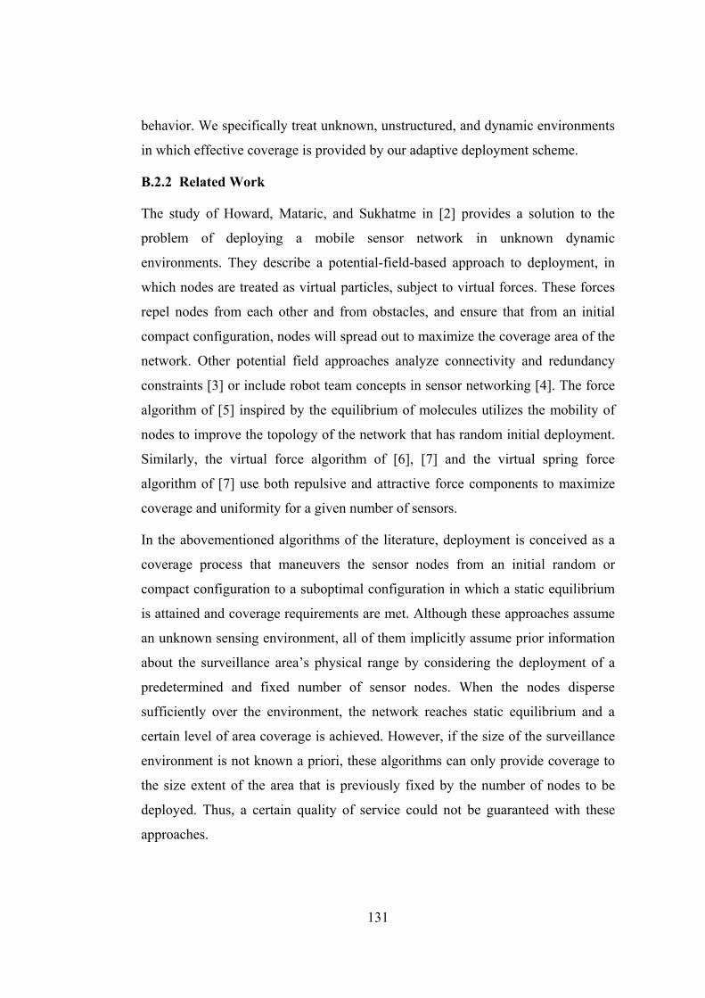
131
behavior. We specifically treat unknown, unstructured, and dynamic environments
in which effective coverage is provided by our adaptive deployment scheme.
B.2.2 Related Work
The study of Howard, Mataric, and Sukhatme in [2] provides a solution to the
problem of deploying a mobile sensor network in unknown dynamic
environments. They describe a potential-field-based approach to deployment, in
which nodes are treated as virtual particles, subject to virtual forces. These forces
repel nodes from each other and from obstacles, and ensure that from an initial
compact configuration, nodes will spread out to maximize the coverage area of the
network. Other potential field approaches analyze connectivity and redundancy
constraints [3] or include robot team concepts in sensor networking [4]. The force
algorithm of [5] inspired by the equilibrium of molecules utilizes the mobility of
nodes to improve the topology of the network that has random initial deployment.
Similarly, the virtual force algorithm of [6], [7] and the virtual spring force
algorithm of [7] use both repulsive and attractive force components to maximize
coverage and uniformity for a given number of sensors.
In the abovementioned algorithms of the literature, deployment is conceived as a
coverage process that maneuvers the sensor nodes from an initial random or
compact configuration to a suboptimal configuration in which a static equilibrium
is attained and coverage requirements are met. Although these approaches assume
an unknown sensing environment, all of them implicitly assume prior information
about the surveillance area’s physical range by considering the deployment of a
predetermined and fixed number of sensor nodes. When the nodes disperse
sufficiently over the environment, the network reaches static equilibrium and a
certain level of area coverage is achieved. However, if the size of the surveillance
environment is not known a priori, these algorithms can only provide coverage to
the size extent of the area that is previously fixed by the number of nodes to be
deployed. Thus, a certain quality of service could not be guaranteed with these
approaches.

132
In this paper, we present a novel adaptive deployment strategy that can guarantee a
desired level of service quality without any prior information about the
surveillance environment. We present a formalism for modeling a sensor network
itself as a fluid that can penetrate and diffuse into highly unknown and
unstructured terrain.
To our knowledge, mobile sensor networks or robot teams have not been modeled
as fluids by the physical principles of fluid dynamics. A fluid dynamics approach
for multi-robot chemical plume tracing is addressed in [8] where flow variables of
a ‘real’ fluid are measured by a computational sensor grid and the flow direction is
estimated for backward tracing. Another work [9] proposes two gas models. One
of them uses a virtual force approach similar to [5] and [6] whereas the other uses
the kinetic theory of gases to model obstacle avoidance and deals with virtual
couette walls to introduce kinetic energy into the system.
B.2.3 Preliminaries: Governing Equations of Fluid Dynamics
We model a mobile sensor network as an inviscid compressible fluid composed of
individual fluid elements, i.e. sensor nodes. In fluid dynamics, one of the flow
models that we adopt in our approach considers the fluid body as a collection of
flowing infinitesimal fluid elements. It is called the nonconservation form flow
model. With this model, the governing equations for the flow of an inviscid fluid
in two dimensions are expressed as in (1).
:
:
x
y
Du px momentum fDt xDv py momentum fDt y
ρ ρ
ρ ρ
∂= − +∂∂= − +∂
(1)
Equation (1) is called the Euler Equations in which ρ is fluid density, D/Dt is the
substantial derivative, p is fluid pressure, fx and fy are body force components per
unit mass in x and y directions, and u and v are the velocity components of an
infinitesimal fluid element in the respective directions. This equation can be
rearranged in a convenient form as in (2)

133
,
,
1
1
t t t tt t ti i i ii i i xt
it t t t
t t ti i i ii i i yt
i
u u u pu v ft x y x
v v v pu v ft x y y
ρ
ρ
⎛ ⎞⎜ ⎟⎜ ⎟⎝ ⎠⎛ ⎞⎜ ⎟⎜ ⎟⎝ ⎠
∂ ∂ ∂ ∂= − + + +∂ ∂ ∂ ∂
∂ ∂ ∂ ∂= − + + +∂ ∂ ∂ ∂
(2)
by using the open form of the substantial derivative terms and time derivatives
isolated on the left-hand side with spatial derivatives residing on the right-hand
side of the equation. In (2), subscript i and superscript t indicate that the flow
variables u, v, ρ, p, and f belong to the ith element of the fluid at time t. For the
details of fluid dynamics concepts discussed in this paper and derivations of
governing equations, please refer to [10].
B.2.4 A Fluid Dynamics Model for Distributed Self-Deployment
A distributed deployment scheme, which is necessarily sensor node oriented, has
to originate from the interactions of nodes with their neighbors and surrounding
environment. It is the interactions of a fluid element with its surrounding and the
physical principles governing these interactions that shape our fluid dynamics
based deployment strategy. With appropriate adaptations of fluid concepts to
mobile sensor networks, we aim at providing a suitable formalism for our
distributed deployment approach.
We assume in our formalism that sensing coverage area of each sensor node is
determined by its sensing range taken as circular in shape with a certain radius
denoted by Rs. Similarly, the communication coverage is the area bounded by
another circle of radius Rc. Coverage in both of these ranges are deterministic. We
also assume that a sensor node can determine the relative position of its neighbors
that lie within its communication range and at any time a sensor node knows its
velocity vector with respect to a local or global reference. Also, each node is
assumed to be capable of learning the velocities of its neighbors through
communication.

134
Adaptation of Fluid Concepts to Mobile Sensor Networks: We define and
reformulate the counterparts of the flow variables and mathematical expressions
appearing in (2) for a mobile sensor network as follows.
1) Velocity Vector: The velocity vector of a fluid element is directly
analogous to the velocity vector of a sensor node. Thus, the velocity vector of the
ith node (node i) may be denoted by Vit = (ui
t, vit).
2) Local Density: We develop a formula for the local density denoted by ρi
at a node location as
2
1 1
i
id di i
ij ijj
R R nnr r
ρ∈Ν
= + × = +∑
(3)
Here, Rd is the deployment radius (0< Rd ≤ Rc) of a deployment neighborhood Ni
for node i, defined as the set of neighboring nodes j that fall within this range. ni is
the number of elements in this set and rij is the Euclidean distance between node i
and node j. This definition provides a normalized density value that is proportional
to the number of deployment neighbors and inversely proportional to the average
distance between node i and its neighbors. Therefore, given the same number of
elements in set Ni, local density would be higher when nodes are closely located.
On the other hand, if set Ni is empty, density takes the value of 1 to account for
node i itself.
3) Pressure: Pressure is the main driving entity in fluid flow. For a perfect
gas, the equation of state is given by
p RTρ= (4)
where R is the specific gas constant and T is the absolute temperature. While we
keep R as a scaling factor in our formulation, we use T for obstacle avoidance
purposes in such a way that nodes that encounter obstacles in their sensing range
raise their temperature, resulting in a repulsive effect on the nodes due to the
higher pressure region generated along the obstacle surfaces as follows
1 (1 )tiT K= + − (5)

135
where K is defined as in (9).
4) Spatial Derivatives of Flow Variables: In equation (2), we have the
partial derivatives of velocity components and pressure with respect to spatial
dimensions x and y. In computational fluid dynamics, these derivatives are
conventionally calculated on grid or mesh structures using finite difference or finite
element methods. In sensor networks, however, generation of a grid is not practical
due to unevenly distributed nature of sensor nodes. Instead, we formulate a
meshfree method [11] based on deployment neighborhood. We define first-order
finite difference equations of a flow variable denoted by ξ as in (6) for node i to
approximate the spatial derivatives of u, v, and p at a time instant t.
( )
( )
1 cos
1 sin
ti
ti
t tt j iiijt
iji j
t tt j iiijt
iji j
x rn
y rn
ξ ξξ θ
ξ ξξ θ
∈Ν
∈Ν
−∂ =∂
−∂ =∂
∑
∑
(6)
We call these as first-order circular difference equations due to the trigonometric
terms multiplying each difference. Differences are also scaled by inter-nodal
distances and averaged over all neighbors within the deployment radius. Here, θij
denotes the polar angle of node j with respect to the reference frame of node i.
Figure B.2.1 illustrate the variation of the circular weight functions cosθij/rij and
sinθij/rij that determine the emphasis of the flow variable differences. Note in this
figure that θij = tan-1(y/x) and rij = √(x2+y2).
For the partial derivative with respect to the x direction, cosine of the relative
orientation between node i and its neighbors places higher emphasis on neighbors
along the x direction. Similarly, sine of the relative orientation places higher
emphasis on the neighbors along the y direction for the partial derivative with
respect to y.

136
Figure B.2.1 Weight functions for the spatial derivatives
4) Body Forces: In fluid dynamics, a fluid element may be under the effect
of various body forces like gravitational, electric, and magnetic forces. These
forces are incorporated in the governing equations in (1) by fx and fy. Considering a
sensor node as a unit mass element in the network, we modeled fx and fy as force
components acting as control entities guiding each node to preferential coverage
regions or target locations. This enables the guidance of the network navigational
flow towards a particular desired direction when necessary. For example, a desired
patrolling direction determined as a result of the coordination among sensor nodes
may be broadcasted by one of the nodes to impose these body force components.
Alternatively, in a clustered network, each cluster head may direct its cluster to
cover a local target area.
Solution of the Governing Equations: As in computational fluid dynamics, we
computationally obtain the velocity vectors of sensor nodes in the form of time-
marching solutions. For example, take one of the velocity components, u, of node i
and assume that we know the flow variables at time t. Then, this velocity
component at a differential time interval ∆t later takes the value given by the
Taylor series expansion
( )22
2 2t t
t t t i ii i
tu uu u tt t
+Δ ⎛ ⎞⎛ ⎞⎜ ⎟⎜ ⎟⎜ ⎟ ⎜ ⎟⎝ ⎠ ⎝ ⎠
Δ∂ ∂= + Δ + +∂ ∂
(7)

137
The velocity component may simply be approximated by the first two terms in (7)
for which all the necessary information is available by (2) through (6). Thus, the
solutions for the velocity components are obtained as
,
,
1
1
t t tt t t t t ti i ii i i i i xt
i
t t tt t t t t ti i ii i i i i yt
i
u u pu u u v f tx y x
v v pv v u v f tx y y
ρ
ρ
+Δ
+Δ
⎛ ⎞⎛ ⎞⎜ ⎟⎜ ⎟⎜ ⎟⎜ ⎟⎝ ⎠⎝ ⎠⎛ ⎞⎛ ⎞⎜ ⎟⎜ ⎟⎜ ⎟⎜ ⎟⎝ ⎠⎝ ⎠
∂ ∂ ∂= + − + + + Δ∂ ∂ ∂
∂ ∂ ∂= + − + + + Δ∂ ∂ ∂
(8)
Limitations, Initial and Physical Boundary Conditions: The solutions obtained
from (8) for the velocity components may exceed the motion capabilities of sensor
nodes. Hence, we utilize hard-limiters for the magnitudes of both velocity and
acceleration of sensor nodes in case they exceed respective thresholds Vth and ath.
The time-marching solutions in (8) require the initial values of the velocity
components to be known. Any particular solution is dictated by these initial
conditions coupled with the physical boundary conditions imposed by the
environment. The only boundary condition for inviscid fluid flow is identified to
be the requirement that the velocity vector of a fluid element immediately adjacent
to a surface be parallel to this surface. Adaptation of this condition to the motion
of a sensor node is illustrated in Figure B.2.2 where a sensor node is depicted at a
distance d to a surface. Whenever node i detects the surface (d≤Rs), it changes its
velocity through a smooth deviation from the velocity solution imposed by (8)
such that the velocity eventually becomes parallel to the surface. The node is also
repelled by the surface if it is closer than a certain distance. This obstacle
avoidance behavior is achieved by using (9).
'(1 ) , , '
2 's
dK K d d BR d
= + − = = −−
nV V V (9)
where K is the smoothing factor and B is a bias term to determine the minimum
distance that a node is allowed to approach a surface. After applying the boundary
condition, V~ is obtained as the corrected velocity by using an auxiliary vector Vn
normal to the surface tangent.

138
Figure B.2.2 Illustration of the physical boundary condition
Damping Viscosity for Network Connectivity: In order to preserve the
connectivity of the sensor network, some kind of artificial viscosity that we call
damping viscosity is applied on the nodes so that the residual velocity terms
( ),( ti
ti
ti vu=V ) in (8) are scaled by a variable that changes with the average inter-
nodal distance as in (10).
,Dt
ijt t t ii i
c
rF t F C
t R+Δ ⎛ ⎞ ⎛ ⎞
⎜ ⎟ ⎜ ⎟⎜ ⎟⎜ ⎟ ⎝ ⎠⎝ ⎠
∂= + Δ = −∂VV V (10)
Here, F is the damping factor, C is the maximum allowed nodal spacing
proportional to Rc (0<C<1) and D is an adjustment constant for the level of
damping.
Adaptive Deployment: In our formalism, several mechanisms exist for high level
behaviors in order to control the deployment process. First, a constant term R in
(4) along with damping viscosity terms in (10) are available for controlling the
spreading and connectivity of the network. Second, the body force components in
(8) facilitate the penetration of the network into goal directions. Obstacle
avoidance behavior of the nodes is also handled by (5) and (9). As explained in the
next section, our deployment strategy benefits from these control mechanisms to
adaptively deploy a network. For example, according to a specific connectivity
requirement, damping viscosity guarantees the convergence of the network
especially in unbounded environments. In unknown bounded environments, on the

139
other hand, favorable deployment directions can be imposed on the network using
the body forces and evolution status of the network is monitored through pressure
and velocity feedbacks.
A major aspect of our adaptive deployment scheme is that nodes are progressively
injected into the environment at the initial deployment locations. When the
previously deployed nodes spread out, new successors are placed in these initial
locations to attain or preserve a certain density level that is determined based on
the overall density, connectivity, and redundancy requirements of the network.
Convergence of the network to static equilibrium or premature termination of the
deployment process depends on the average of velocity feedbacks from the nodes.
If the network achieves static equilibrium due to connectivity constraint, its
deployment naturally ceases. Whereas, when a certain density or redundancy level
is attained or coverage requirements are met, injection of new nodes into the
environment may temporarily or permanently be stopped.
B.2.5 Simulation Results
We investigate the performance of our approach in terms of coverability,
scalability, and robustness. Since we assume unknown environments, our
coverability and scalability measure is the variation of covered area with respect to
deployed node number. Robustness is analyzed in presence of localization
uncertainty and node failure. Parameter settings of our simulations are indicated in
Table B.2.1 with reference to the related figure numbers.
To illustrate the obstacle avoidance and guided penetration capabilities of the
sensor nodes, we deploy a simple network composed of 9 nodes as shown by black
dots in Figure B.2.3. In this simulation, assume that each node is equipped with a
GPS device and the coordinates of a target point are given as indicated by the
bigger red dot in Figure B.2.3. Thus, each node assumes a body force towards the
target which is a virtual force sink. The final configuration attained after 30
simulation time units is shown by the white dots in the same figure. White
streamlines tailing behind each node show the deployment trajectories. This
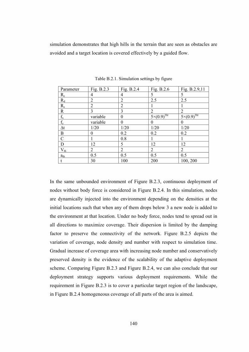
140
simulation demonstrates that high hills in the terrain that are seen as obstacles are
avoided and a target location is covered effectively by a guided flow.
Table B.2.1. Simulation settings by figure
Parameter Fig. B.2.3 Fig. B.2.4 Fig. B.2.6 Fig. B.2.9,11 Rc 4 4 5 5 Rd 2 2 2.5 2.5 Rs 2 2 1 1 R 3 3 2 2 fx variable 0 5×(0.9)20t 5×(0.9)20t
fy variable 0 0 0 ∆t 1/20 1/20 1/20 1/20 B 0 0.2 0.2 0.2 C 1 0.8 1 1 D 12 5 12 12 Vth 2 2 2 2 ath 0.5 0.5 0.5 0.5 t 30 100 200 100, 200
In the same unbounded environment of Figure B.2.3, continuous deployment of
nodes without body force is considered in Figure B.2.4. In this simulation, nodes
are dynamically injected into the environment depending on the densities at the
initial locations such that when any of them drops below 3 a new node is added to
the environment at that location. Under no body force, nodes tend to spread out in
all directions to maximize coverage. Their dispersion is limited by the damping
factor to preserve the connectivity of the network. Figure B.2.5 depicts the
variation of coverage, node density and number with respect to simulation time.
Gradual increase of coverage area with increasing node number and conservatively
preserved density is the evidence of the scalability of the adaptive deployment
scheme. Comparing Figure B.2.3 and Figure B.2.4, we can also conclude that our
deployment strategy supports various deployment requirements. While the
requirement in Figure B.2.3 is to cover a particular target region of the landscape,
in Figure B.2.4 homogeneous coverage of all parts of the area is aimed.

141
Figure B.2.3 Obstacle avoidance and guided penetration of nodes into the landscape
Figure B.2.4 Self-spreading of nodes
In a bounded environment as shown in Figure B.2.6, deployment of an adaptively
changing number of nodes is considered next to examine the coverability,
scalability, and fault tolerance of the approach. In this figure, initial deployment
locations are indicated by black points where nodes are progressively injected into
the environment with a certain initial condition (V0=(2,0)) to direct the nodes into
the environment. Also, an initial body force that quickly diminishes with time (see
Table B.2.1) is applied on the newly deployed nodes as an injection force that
prevents their immediate backward escape out of the environment. To account for
uncertainty, we introduce an additive Gaussian noise for the neighbor localization
of each node. Using a zero mean and 0.05 variance Gaussian noise, the final
configuration of the network is depicted Figure B.2.6. The same simulation is
repeated with no noise for the comparison of the resulting coverability
characteristics as given in Figure B.2.7. From the variation of coverage with

142
respect to node number, it can be seen that coverage increases with increasing
number of nodes until it saturates at a certain level where the environment is fully
covered. This also shows that our deployment scheme is scalable in terms of
network and environment size. It is seen from Figure B.2.7 that the same coverage
can be provided in presence of localization error but with deploying more sensors
than the noiseless case. In Figure B.2.8, variations of average node velocity and
density (with 0.01 noise variance) are plotted. As the density increases, velocities
of nodes drop and the network flow slows down due to increased nodal
interactions and damping viscosity. Note the transient fluctuations in both plots
with magnitudes that clearly decrease after approximately t=100. This moment in
Figure B.2.7 corresponds to the time when the coverability starts saturating.
Figure B.2.5. Variation of coverage, density, and node number with time in Figure B.2.4
To demonstrate the fault tolerance and adaptivity of the approach to node failures
and terrain dynamics, we analyse a scenario in which some hills appearing as
obstacles in the environment collapse, destroying 14 nodes already positioned in
the surrounding area. The destroyed portion of the terrain and the failing nodes
buried under the debris are enclosed in the white rectangle as shown in Figure
B.2.9 just before the downfall. Figure B.2.10 shows the destruction of these 14
nodes (out of 86) resulting in an immediate decrease in coverage by 21% (from

143
122.8 to 97.0 unit squares). However, the network recovers from this situation
within 10 time units and covers the new area that is created as a result of landscape
change as shown in Figure B.2.11.
Figure B.2.6 Adaptive deployment in a bounded environment
Figure B.2.7 Variation of coverage and node number with time in Figure B.2.6

144
Figure B.2.8 Variation of node velocity and density with time in Figure B.2.6
Figure B.2.9 Area and nodes to be destroyed at t=100
Figure B.2.10 Recovery from node failure in Figure B.2.9 due to collapse of an area

145
Figure B.2.11 Response to dynamical change of the terrain and new coverage of the destroyed area in Figure B.2.9
B.2.6 Conclusion
We address adaptive self-deployment of mobile sensor networks in unknown,
unstructured, and dynamic environments. A novel distributed strategy based on a
fluid dynamics model is developed and several desirable properties are achieved in
terms of coverability, scalability, and robustness. While coverability and
robustness are achieved as a result of the self-spreading behavior of the network,
distributed nature of the approach provides scalability in terms of network and
environment size. Also, diffusive movement of sensor nodes facilitates effective
operation of the network in unstructured terrain. Simulation results showed that
our adaptive scheme provides effective deployment and coverage in unknown
dynamic environments. It can efficiently be utilized in the surveillance of an entire
area as well as to cover target regions individually. It is also tolerant to localization
error in neighborhood interactions and failure of nodes under harsh environment
conditions.
B.2.7 References
[1] S. Meguerdichian, F. Koushanfar, M. Potkonjak, M. Srivastava, “Coverage Problems in Wireless Ad-hoc Sensor Networks,” in Proceedings of IEEE Infocom, 2001, pp. 1380-1387.
[2] Howard, M. J. Mataric, G. S. Sukhatme, “Mobile Sensor Network Deployment using Potential Fields: A Distributed, Scalable Solution to the

146
Area Coverage Problem,” in Proceedings of the 6th International Symposium on Distributed Autonomous Robotics Systems, Japan, June 2002.
[3] S. Poduri, G. S. Sukhatme, “Constrained Coverage for Mobile Sensor Networks,” in Proceedings of the 2004 IEEE International Conference on Robotics and Automation, New Orleans, LA, April 2004.
[4] O. Popa, C. Helm, “Robotic Deployment of Sensor Networks Using Potential Fields,” in Proceedings of the 2004 IEEE International Conference on Robotics and Automation, New Orleans, LA, April 2004.
[5] N. Heo, P. K. Varshney, “A Distributed Self Spreading Algorithm for Mobile Wireless Sensor Networks,” in Proceedings of IEEE Wireless Communications and Networking Conference, 2003.
[6] Y. Zou, K. Chakrabarty, “Sensor Deployment and Target Localization Based on Virtual Forces,” in Proceedings of IEEE Infocom Conference, vol. 2, 2003.
[7] Shucker, J. K. Bennett, “Scalable Control of Distributed Robotic Macrosensors,” in 7th International Symposium on Distributed Autonomous Robotic Systems, June 2004.
[8] Zarzhitsky, D. R. Thayer, “A Fluid Dynamics Approach to Multi-Robot Chemical Plume Tracing,” in Proceedings of AAMAS’04, New York, USA, July 2004.
[9] W. Kerr, D. Spears, W. Spears, D. Thayer, “Two Formal Fluid Models for Multi-agent Sweeping and Obstacle Avoidance,” Lecture Notes in Computer Science, vol. 3228, Springer-Verlag, 2004.
[10] J. D. Anderson, Computational Fluid Dynamics: the Basics with Applications, McGraw-Hill, 1995.
[11] R. Liu, Mesh Free Methods: Moving Beyond the Finite Element Method, CRC Press, 2002.
B.3 Control of Robotic Swarm Behaviors
Publication: To Appear in Proceedings of the 2007 IEEE/RSJ International
Conference on Intelligent Robots and Systems (IROS), San Diego, CA,USA, Oct.
29-Nov. 2, 2007.
Title: Control Robotics Swarm Behaviors Based on Smoothed Particle
Hydrodynamics
Authors: Muhammed R. Pac, Aydan M. Erkmen, Ismet Erkmen.

147
Abstract: The paper presents a fluid dynamics based framework for the control of
emergent behaviors of robot swarms that are modeled as fluids. A distributed low-
level control mechanism is developed based on Smoothed Particle Hydrodynamics
(SPH) and it is coupled with a high-level control layer that is responsible for the
tuning of fluid parameters to generate desired behaviors from the swarming
characteristics of the robots. It is shown by simulations that using the same low-
level SPH formalism, different swarming behaviors can emerge from the local
interactions of robots according to the settings of the fluid parameters that are
controlled by the high-level control layer.
B.3.1 Introduction
Swarm robotics aims at developing scalable, flexible, and robust coordination
mechanisms to control large groups of autonomous mobile agents. It is inspired by
ethological phenomena in which swarms of animals (insects, fishes, birds, etc.)
interact to coordinate their actions, create collective intelligence, and perform tasks
that are far beyond the capabilities of individual members. Absence of central
control in these behaviors and emergence of cooperation from only local
interactions makes social swarms highly fault-tolerant, scalable, and adaptive to
changing conditions. It is these inherent properties of biological swarms, which are
also desirable for collective robotics, that attract a growing interest among
researchers [1],[2].
Approaches currently available in the literature to swarm robotics generally base
their formalism on the underlying biological phenomena and try to mimic the
behaviors of animals in their artificial or simulated counterparts [3]–[5]. In these
studies, adaptation of animal behaviors to multi-robot systems as a low-level
coordination mechanism is mainly addressed. While constructing large numbers of
autonomous robots is already a big challenge, developing control algorithms
applicable to such systems based on the behaviors of animal swarms remains to be
the main focus of the recent research.
In this paper, we propose a novel model that notably helps in controlling emergent
and aggregate swarming behaviors of large-scale multi-robot systems. In contrast

148
to the majority of approaches in the literature inspired by coordination in animal
swarms, we base our formalism on the physics of fluids through an analogy
between swarm robots and fluid particles. Our control methodology leads us to
achieve desirable properties such as decentralized coordination, scalability, and
robustness by applying the physical principles behind the dynamics of fluids to the
distributed control of swarm robots. For the numerical analyses of the governing
equations of fluid dynamics, we use Smoothed Particle Hydrodynamics (SPH)
method [6]. Contrary to the conventional grid (or mesh) based analyses, SPH is a
meshfree method that we found particularly suitable for our purposes of modeling
a robot swarm as a collection of fluid particles.
B.3.2 Previous Work
Apart from the popular “artificial potential field” approach to the control of multi-
robot systems [5], [7], [8], there appears another line of research inspired from
physics laws to solve problems such as coverage, surveillance, formation control,
and obstacle avoidance. The most notable studies in this context are works by W.
Spears and D. Spears, who proposed a “physicomimetics” framework for the
distributed control of swarms of robots [9], [10]. In this framework, individual
robots are treated as particles subject to artificial physics force laws. Similar to the
potential field approach, the mobile robots are driven by these virtual forces and
eventually the system is expected to achieve a desired configuration which
minimizes the overall system potential energy. Depending on the relative strengths
of the attractive and repulsive forces between particles, the system acts like a solid,
liquid, or gas. This approach was used to address the lattice formation problem.
For the coverage problem, on the other hand, they proposed a “kinetic theory”
approach in which the problem is handled as the sweeping of a corridor by a
particle swarm [11]. Shimizu et al. [13] proposed to use Stokesian Dynamics in
designing local interactions of robots to maintain the coherence of the swarm in
unstructured environments.
The work by Perkinson and Shafai [14] proposes to utilize SPH so that the
members of a nanorobot swarm can be controlled as fluid particles. Obstacle

149
avoidance and coverage problems are addressed in 2D simulation environments.
To the best of our knowledge, this is the only work using SPH as a motion control
algorithm for multi-robot systems. However, it does not establish an analogy
between fluids and robot swarms and limits the method to the self-deployment of a
sensor network in an unknown environment.
In the works by Pac et al. [15], [16], the authors extended the idea of physics-
based approaches by modeling a robot network as a fluid body and controlling the
deployment process through the parameters available in the governing equations.
They used a custom defined meshfree particle method for the numerical solution
of the equations. Primarily addressing the coverage of unknown unstructured
environments with mobile sensor networks, they demonstrated how the
configuration of the network can be changed to satisfy connectivity requirements
and analyzed the robustness of the approach in response to dynamical environment
and network conditions.
In this paper, we further extend the previous formalism in [15] by developing a
low-level, fluid dynamics based control model to coordinate the local interactions
of robots while providing an interface composed of flow parameters to higher level
algorithms for controlling the global behavior of the system. We exploit SPH for
the modeling and analysis of robot swarms through the set of fluid dynamics
equations. We demonstrate the validity and promise of the approach by applying it
to common problems recurring in the swarm robotics literature.
B.3.3 Proposed Control of Robotic Swarm Behaviors
In this section, we present our motivation in developing a fluid dynamics based
model for the distributed control of robot swarms. When a fluid body is considered
as a collection of infinitesimal fluid elements, the analogy between these elements
and the individuals in a swarm becomes more apparent. There are various
characteristics of fluids that are desirable in a robot swarm. For example, the
obstacle avoidance and source-to-sink optimal path finding behavior of fluids
inspired quite a few works in mobile robotics area [17]–[20]. Similarly,
harmonious and self-coordinated movement of fluids is also desirable in robot

150
swarms. While obstacle avoidance is in part a local reactivity of the fluid,
coherence of the whole body is a result of the aggregate state of it. It can be seen
that these properties exist at conceptually two distinct scales of a fluid: one is the
particle scale that explains the local interactions of a fluid element with its
surrounding, and the other is the macroscopic scale where the global motion of the
fluid can be described. It is a fact that the overall motion of a fluid essentially
emerges from the local interactions of particles in it and the principles governing
these interactions are based on various physical quantities such as viscosity,
compressibility, and temperature. Our idea in this paper is to utilize these
quantities to ‘control’ the swarming behaviors of a multi-robot system that we
model as a collection of fluid particles with quite the same mathematical
formalism of SPH. Our flexibility in using this formalism is that we can change
any parameters of the model in such a controlled way that the desired swarming
behaviors are obtained.
Towards this aim, we developed a control architecture with two fundamental
layers such that the lower layer deals with the particle scale of the swarm while the
upper layer controls the macroscopic behavior. The two layers are in coordination
through an interface composed of fluid parameters that are described by the SPH
model of the swarm in the lower layer. By this way, the global behavioral control
of the swarm is designed in terms of the fluid parameters and programmed into a
high-level control algorithm in the higher layer; whereas the local interactions of
robots are governed by the SPH based low-level fluid model operating with this
parameter setting and controlled through the interface (Figure B.3.1). Here, we
need to emphasize that the overall behavior of the swarm still emerges from the
local interactions of the robots but this happens under the control of the associated
fluid parameters that are designed and adjusted for the particular task.

151
Figure B.3.1 Separate layers controlling the local interactions and global behavior in a decentralized system
Figure B.3.1 depicts the relationships with bidirectional arrows between the
control layers and interactions of the robots with each other and with the
environment. The low-level control layer is called the SPH Layer which inherently
exhibits swarming behaviors, whereas the high-level control layer is called the
Swarm Control Layer. While this separation does not violate the decentralized
nature of the commonly adopted swarm approach, the high-level control layer can
also be implemented as an off-site central controller unit of the swarm where the
global operation of the swarm is planned and resulting control commands are sent
to the low-level control layer through the interface in between. We illustrate this
architectural case in Figure B.3.2.
Figure B.3.2 Global behavior control in a central unit
The majority of collective robotics applications require the incorporation of a
central facility to control, monitor, or at least to initialize the on-site distributed

152
system. Hence, while we agree with the notion of emergent swarm behavior
emanating from local interactions, we also believe in the benefit of utilizing
centralized mechanisms along with it, whenever necessary and suitable. Separating
the control of emergent swarm behaviors from the underlying swarm
characteristic, which is the fluid model in our case, makes the modular
combination of these two paradigms –centralized and decentralized– possible.
As mentioned, the interface between the swarm control layer and the SPH layer is
composed of the flow parameters that can be artificially set to desired values so
that a particular swarm behavior emerges. Elements of this interface are of two
types: those inherently available in the fluid dynamics equations and those
belonging to the swarm systems based on SPH. These parameters are summarized
in Table B.3.1 and discussed in the next section. Although this is not an exhaustive
list of factors involved in the flow process, optimal design of a swarm for a
particular task is already challenged by the tuning of these basic parameters as we
show in the simulation results.

153
Table B.3.1 Interface Parameters Between Swarm Control and SPH Layers
Parameter Variation Description Parameters from Fluid Physics
Compressible Gas-like swarms Compressibility Incompressible Liquid-like swarms Viscous: dynamic viscosity
Shear and normal stresses in robot-robot and robot-environment interactions
Viscosity ( μ )
Inviscid No shear and normal stresses Available: static, dynamic
Provides directional flow Body force ( f )
Not available Self-spreading of gas-like swarms Gas Constant (R) For gas-like swarms Effects inter-particle repulsion Initial density (ρ0) For liquid-like swarms Effects inter-particle repulsion Temperature (T) For gas-like swarms Facilitates obstacle avoidance Parameters from SPH model of Swarm Robots
Static Fixed swarm size Deployment Mode Adaptive Dynamically changing swarm size
adaptive to requirements Support Domain Size (Rd )
Deployment radius Adjusts the range of local interactions
Kernel Function Gaussian, spline, quadratic, etc.
Defines the weights of interactions with neighbors
Average particle spacing Determines redundancy profile of gas-like swarms
Connectivity
Initial density, stiffness constant
Involves in patterns of liquid-like swarms
Normal velocity damping factor
Strength of the repulsive force normal to obstacles
Obstacle Avoidance
Approach bias Limitation of minimum distance to obstacles
B.3.4 SPH Formulation of Robots
Preliminaries: In order to develop a generic control approach to robot swarms
which may range from nanorobots to autonomous underwater vehicles and to
unmanned aerial/ground vehicles, we present the SPH formulation in the most
general form representing 3D flow of a viscous fluid (liquid or gas) in presence of
body forces. Then, the relevant form of the governing equations is called the
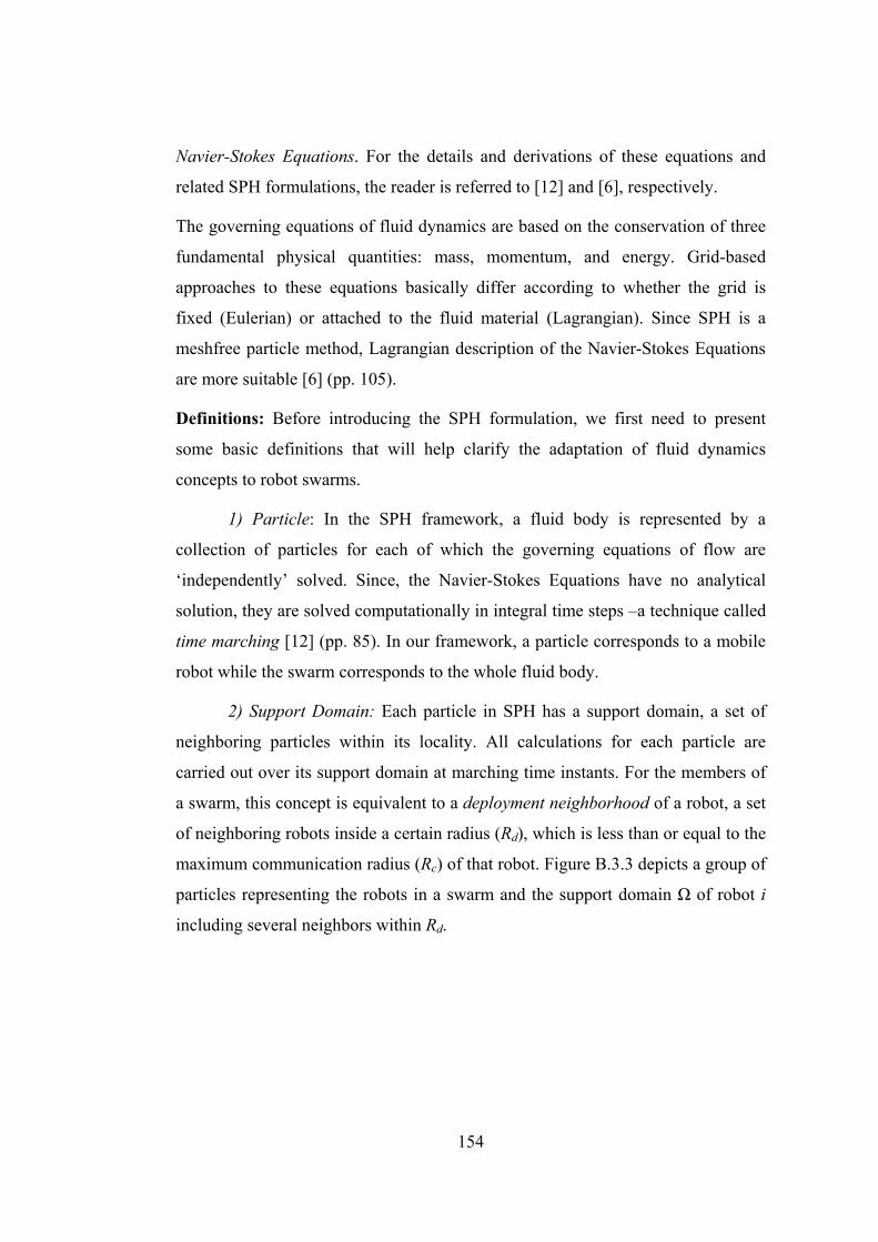
154
Navier-Stokes Equations. For the details and derivations of these equations and
related SPH formulations, the reader is referred to [12] and [6], respectively.
The governing equations of fluid dynamics are based on the conservation of three
fundamental physical quantities: mass, momentum, and energy. Grid-based
approaches to these equations basically differ according to whether the grid is
fixed (Eulerian) or attached to the fluid material (Lagrangian). Since SPH is a
meshfree particle method, Lagrangian description of the Navier-Stokes Equations
are more suitable [6] (pp. 105).
Definitions: Before introducing the SPH formulation, we first need to present
some basic definitions that will help clarify the adaptation of fluid dynamics
concepts to robot swarms.
1) Particle: In the SPH framework, a fluid body is represented by a
collection of particles for each of which the governing equations of flow are
‘independently’ solved. Since, the Navier-Stokes Equations have no analytical
solution, they are solved computationally in integral time steps –a technique called
time marching [12] (pp. 85). In our framework, a particle corresponds to a mobile
robot while the swarm corresponds to the whole fluid body.
2) Support Domain: Each particle in SPH has a support domain, a set of
neighboring particles within its locality. All calculations for each particle are
carried out over its support domain at marching time instants. For the members of
a swarm, this concept is equivalent to a deployment neighborhood of a robot, a set
of neighboring robots inside a certain radius (Rd), which is less than or equal to the
maximum communication radius (Rc) of that robot. Figure B.3.3 depicts a group of
particles representing the robots in a swarm and the support domain Ω of robot i
including several neighbors within Rd.
155
Figure B.3.3 Illustration for the support domain Ω of robot i
3) Smoothing (Kernel) Function: In SPH, the state of a fluid is represented
by a set of particles that posses individual particle properties and move according
to the governing equations. Numerical discretization is made by approximating the
values of field functions, their derivatives, or integrals at these particle locations
where neighboring particles contribute to the particle approximations based on
their influence on the location. It is the smoothing function that determines the
values of these contributions. The SPH formalism starts with the following
identity, where Ω is the volume of the integral containing the position vector x.
( ) ( ) ( )f f dδΩ
= −′ ′ ′∫x x x x x (1)
As an approximation to the above Dirac delta function δ, a smoothing kernel is
used in the integral representation of the flow equations as in (2) where W is the
smoothing function and h is the smoothing length. The angle brackets designate
that the integral representation is an approximation.
( ) ( ) ( )f f W h dΩ
< >= −′ ′ ′∫x x x x , x (2)
In our formalism, we use the Gaussian kernel for its closed form expression and
accuracy in disordered particles [6] (pp. 63). The kernel is given in (3) to (5),
where R is a scaled distance between the particle for which the kernel is being
computed and its neighbors in the support domain. The smoothing length h defines
the influence area of the smoothing function along with κ, a user-defined constant
that determines the radius of deployment neighborhood. Figure B.3.4 and Figure

156
B.3.5 are the respective shapes of the 2D Gaussian kernel and its derivative that
we use in our model.
2
( , )0
Rd de R RW R h
otherwiseα −⎧⎪⎨⎪⎩
≤= (3)
2
3 2 31 21 3d
h D flowh D flow
παπ
⎧⎪⎨⎪⎩
= (4)
drR h and Rh
κ= =
(5)
Figure B.3.4 The compact Gaussian kernel in 2D over the support domain
Figure B.3.5 Derivative of the Gaussian Kernel with respect to the horizontal spatial axis
157
The SPH Formulation: In our SPH formalism, each robot in the swarm
represents a computational element where the conservation of momentum equation
is independently solved for the velocity of that particular robot based on the local
information within its support domain. Therefore, the computational method is
naturally distributed and massively parallel. The particle approximations for the
fluid dynamics equations of density and momentum in (6) and (7) along with (8)-
(9) are adapted from [6] (pp. 113–123). In these equations, ρ stands for density, m
for mass, and v for the velocity vector of the particle i. In the text, we denote vector
values in bold face. Since a particle corresponds to a single member of the swarm
in our approach, the density at the location of a robot is equivalently formulated by
the weighted sum of the neighbor masses in the support domain as in (6), where
the weighting function is the smoothing kernel indeed. As for the mass, we take it
as unity for all robots although it may also be used to attribute more weight to
some of the robots to introduce heterogeneity in the swarm. In (7), f is the body
force vector acting on unit mass [12] (pp. 61). In fluid physics, a typical body
force is the gravitation, whereas the high-level control layer of our approach uses it
artificially to impose a preference in the direction of flow whenever relevant to the
desired swarming behavior. In the superscripts, α and β are used to denote the
spatial dimensions x, y, and z. Wij is the kernel evaluated for robot i and its
neighbor j. D/Dt is the total derivative operator [12] (pp. 43) with respect to time
and ∂/∂xβ is the partial derivative with respect to the spatial dimension denoted by
β. σ is the total stress tensor given by (8), where p is the pressure multiplied by the
delta function (δαβ = 1 if α = β, 0 otherwise) and summed with the viscous shear
stress τ defined in (9). Finally in (9), μ is the dynamic viscosity and is zero for
inviscid flow. We use these concepts in our formalism without redefinition to
obtain the natural characteristics of fluids in our model. However, all of the
parameters involved in these equations are adjusted by the swarm control layer to
generate a desired swarming behavior.
The total stress tensor σ describes the interactions among particles. For instance,
pressure is a potential field in a global view and produces inter-particle repulsion
that results in flow toward homogeneous distribution. It is exactly the same effect

158
of pressure that we employ in our approach to control the uniform distribution of
the swarm. Shear stress τ, on the other hand, is a viscous effect that tries to
regulate the velocity field by producing inter-particle and particle-obstacle drag
forces. In our approach, these are analogous to attractive forces around a robot
such that each neighbor and obstacle in the vicinity imposes its own velocity on
that robot. Therefore, total stress tensor is the main driving entity of swarm flow
and of harmony among robots.
i
i j ijj
m Wρ∈Ω
= ∑
(6)
i
i j ijij i
j i j i
WD mDt
αβ αβαα
βσ σ
ρ ρ∈Ω
+ ∂= +
∂∑v fx
(7)
pαβ αβ αβσ δ τ= − +
(8)
( )23
β ααβ αβ
α βτ μ δ⎛ ⎞⎜ ⎟⎜ ⎟⎝ ⎠
∂ ∂= + − ∇⋅∂ ∂v v vx x (9)
For β in (7), the summation is taken over repeated dimension indices. For 2D flow,
for example, equations (7)-(9) can be rewritten in an expanded form as in (10)-
(11).
i
i
xy xyxx xxi j ij i j ij xi
j ij i j i i j i
xy xy yy yyi j ij i j ij yi
j ij i j i i j i
W WDu m fDt x y
W WDv m fDt x y
σ σσ σρ ρ ρ ρ
σ σ σ σρ ρ ρ ρ
∈Ω
∈Ω
⎛ ⎞⎜ ⎟⎜ ⎟⎝ ⎠⎛ ⎞⎜ ⎟⎜ ⎟⎝ ⎠
++ ∂ ∂= + +
∂ ∂
+ +∂ ∂= + +
∂ ∂
∑
∑ (10)
223
223
xx i i ii i i
xy i iii
yy i i ii ii
u u vpx x y
v ux y
v u vpy x y
σ μ
σ μ
σ μ
⎛ ⎞⎛ ⎞⎜ ⎟⎜ ⎟⎜ ⎟⎝ ⎠⎝ ⎠
⎛ ⎞⎜ ⎟⎝ ⎠
⎛ ⎞⎛ ⎞⎜ ⎟⎜ ⎟⎜ ⎟⎝ ⎠⎝ ⎠
∂ ∂ ∂= − + − +∂ ∂ ∂
∂ ∂= +∂ ∂
∂ ∂ ∂= − + − +∂ ∂ ∂
(11)

159
In (10), u and v are the velocity components in x and y directions, respectively, of
robot i and are what we ultimately need to find out for each robot. As for the
pressure, there are two definitions according to the fluid being compressible (gas)
or incompressible (liquid). The compressible case is modeled as in (12) where
pressure is a function of density through the state equation of gases [12] (pp. 79).
R and T are the specific gas constant and the absolute temperature, respectively.
Qualitatively, (12) is the statement of the fact that pressure is linearly related with
density within a certain volume or area. The unit area in our case is the support
domain of each robot where increased number of neighboring robots results in an
increase in the pressure at that particular location. This linear relationship involves
a constant R and a variable T. We use R as a swarm specific parameter to adjust
the inter-robot repulsion due to pressure. In obstacle-laden environments, for
example, R can be reduced to allow close spacing of robots without producing
excessive pressure while moving across narrow passages. T, on the other hand, is
used as a secondary mechanism of obstacle avoidance (The primary mechanism is
the boundary conditions described in part D) in a way that when a robot
encounters an obstacle, it raises its temperature and produces higher pressure at its
location so that its neighbors are distracted from the obstacle without coming
across with it. This also remedies a numerical boundary problem called particle
deficiency [6] (pp. 138) by compensating for the unrealistically reduced pressure at
boundaries.
For incompressible flow, it is a fact that density inside a liquid is constant and is
not a function of pressure. However, due to the inefficiency in solving for the
actual state equation of liquids, the computational fluid dynamics community has
adopted to use artificial compressibility concept that practically models
incompressible fluids [6] (pp. 136). Here, we also formulate incompressible flow
by using the artificial compressibility definition of [21] as given in (12) where ρ0
stands for the initial or desired density of the liquid, whereas k is the stiffness
constant. The greater k is, the more accurate incompressibility is simulated but in
expense of smaller time steps for processing due to the requirements of increased
pressure values. For a wireless swarm system, therefore, the value of k is limited

160
by the bandwidth of local communication among robots because each robot needs
to communicate with its neighbors and collect flow information to process its
equations at each time step.
( )0
Compressible Flow :Incompressible Flow:
i i i i
i i
p R Tp k
ρρ ρ
=
= −
(12)
The apparent difference between compressible and incompressible flow benefits to
different application scenarios in a swarm system. For example, compressible flow
is suitable for tasks that require the coverage of an area because the self-spreading
behavior of gases is desirable in a mobile surveillance system. On the other hand,
incompressible flow is more appropriate for patrolling and flocking tasks that
require stiff formations among robots along a track.
Solution of the Momentum Equation: Solutions to the flow equations are
obtained using the time-marching technique. It is actually an integration of the
first-order Taylor series approximation of velocity over time to evolve its value as
in (13).
tDt t t i ti i Dt
⎛ ⎞⎜ ⎟⎜ ⎟⎝ ⎠
+Δ = + Δv
v v
(13)
Since we assume robots as point particles, we do not deal with any dynamics of
the robot. Depending on the application and the type of robots, it is the particular
locomotion controller of the robot that accepts the velocity controls in (13) and
deals with the physical dynamics.
Despite the very same equations are employed, different flow patterns are
observed in different environments due to the varying initial and boundary
conditions for the particular case. Initial conditions refer to the initial velocities
and locations of the robots, whereas boundary conditions are imposed by the
environment surrounding the robots. Thus, the source of the robot-environment
interactions is the obstacles within the deployment terrain. The characteristic
obstacle-avoidance behavior of fluids is modeled in our approach through the
associated boundary conditions such that for inviscid flow (μ = 0), the only

161
boundary condition is that the velocity of a robot adjacent to a surface is parallel to
it. For viscous flow (μ > 0), there is an additional no-slip condition such that the
velocity of the robot reduces to zero at the immediate vicinity of the surface.
We utilize a simple mechanism to satisfy these conditions as follows. First, we
assume that the information obtained from the sensors of the robot due to an
obstacle basically carries range and bearing data of an obstacle point in space
relative to the robot. Also, if the robot has multiple sensors around its perimeter or
a scanning detector, it is highly probable that it detects more than one point of an
obstacle almost at the same time as illustrated in Figure B.3.6. Then, it can reason
about a surface and adjust its velocity according to the boundary condition such
that the velocity component perpendicular to the surface is decreased with
decreasing distance to the obstacle. If the robot happens to detect only one obstacle
point, then it can assume the surface normal to originate from this point passing
through its own location.
(x1, y1)
(x2, y2)
v = (u,v)
d
(x12, y12)
(x0, y0)φ
Obstacle surface
Robot
vp
Figure B.3.6 Obstacle avoidance through boundary conditions
Equation (14) briefly formulates the boundary condition such that the velocity
component perpendicular to the surface decreases with decreasing k value, a
measure of distance to the obstacle. The parallel component of velocity vp to the
surface can be derived from the three locations (x0, x1, and x2) in Figure B.3.6. In
the expression of k below, Rs represents the sensing range of the robot beyond
which the robot cannot detect obstacles.

162
(1 ) , (2 )k k k d R dsp′ = + − = −v v v
(14)
Besides these conditions from fluid dynamics, there are other conditions
originating from the nature of swarm robotics or from the task requirements. For
example, the members of a swarm have limited mobility capabilities which may
not fully satisfy the direct solution obtained from flow equations for all time
instances. In our model, robot velocities are clipped by hard-limiters whenever the
flow solution exceeds these limits. Robots also need to preserve the wireless
connectivity among each other so that no robot detaches from the swarm. We
addressed this condition in [15] by using a damping factor to slow down the
outliers in the swarm. In this work, we also use the viscous stress among the
particles to preserve their integrity.
B.3.5 SPH Based Swarm Characteristic
In this section, we present sample results from our numerous simulations chosen to
address some ‘standard’ problems in swarm robotics literature in order to
demonstrate the capabilities and potential use of our SPH based control strategy
for swarm behaviors.
Deployment and Coverage: In our previous work [16], we addressed the
deployment problem of mobile sensor networks in unknown, unstructured,
dynamic environments with an emphasis on the robustness of self-deployment and
coverage in response to changing terrain and network conditions. The sensor
network was modeled as an inviscid gas and the self-spreading behavior of gases
was exploited for coverage tasks.
Here, this first simulation aims to analyze the effect of viscosity (μ) on coverage as
it is varied as an interface parameter. We simulate the compressible fluid model of
a robot swarm in a corridor sweeping task (Figure B.3.6). We use the body force
parameter f set to 0.5 Newton toward the right so that the robots released from the
left hand side of the corridor sweep through to the right while covering spare areas
and avoiding obstacles. Introduction of viscosity into the flow is expected to result
in frictional loss and hence a slower movement especially around obstacles. The

163
plot in Figure B.3.7 typically shows that the coverage per robot is less when
viscosity is nonzero. From Figure B.3.8, it is seen that the average velocity of the
robots is reduced under friction. However, reduction in coverage per robot can
better be explained with the increased average robot density when viscosity is
nonzero as shown in Figure B.3.9. Therefore, it can be concluded that increased
viscosity results in slower deployment, whereas it increases the average density of
the robots. Although this is not the primary mechanism of controlling the overall
density of the robots in the swarm, which is discussed in the last simulation, it can
be utilized as a mechanism of slowing the movement down around points of
interest in the terrain that require more careful inspection and are virtually
assumed as obstacles by the robots.
Figure B.3.6 Flow of robots from left to right in an obstacle-laden corridor
Figure B.3.7 A typical comparison of coverage per robot for inviscid (μ = 0.0 mPa.s) and viscous flows (μ = 0.1 mPa.s)

164
Figure B.3.8 Average velocities of robots under zero and nonzero viscosity
Figure B.3.9 Average densities of robots under zero and nonzero viscosity
Patrolling and Dispatching: In our SPH model, there are several flow parameters
suitable for utilization in tasks that require a guided motion of a swarm of robots
toward a target along a predefined route through passages. Some applications
involve such tasks as autonomous security patrolling and vehicle dispatching.
Body force f is the parameter that plays the most important role in this respect. In
the previous corridor sweeping example, body force was constant in magnitude
and direction and was used to direct the swarm to the right of the corridor. For a
patrolling or dispatching task, however, a position-varying body force has to be
used. An example to such tasks is the dispatching of autonomous ground vehicles
(AGV) in outdoor terrains based on a predetermined route and GPS data. Also, the
compressibility parameter adjusted for incompressible flow becomes appropriate
to gather and funnel down the robots along a specified route since liquids do not
spread out as gases do.

165
Figure B.3.10 shows an autonomous dispatching scenario, where robots are given
5 waypoints (coordinates of terrestrial points) by the swarm control layer in the
terrain to navigate through. Upon arrival of a waypoint, each robot updates the
body force guiding its motion to head toward the next waypoint. It is shown in this
simulation that for tasks requiring a directed movement of the swarm in
unstructured terrains, utilizing a dynamically changing body force parameter is
effective. Moreover, modeling the swarm as a liquid rather than a gas is
particularly beneficial in keeping the robots on a thin track.
Figure B.3.10 Dispatching of robots through waypoints in a rural terrain
Flocking and Formation Control: Flocking is the synchronized and harmonious
movement of a collection of agents as a single body –a behavior demonstrated by
flocks of birds, schools of fishes, etc. While it has been modeled as an emergent
distributed behavior [22] inspiring from flocks of animals, flocking is inherently
available in the nature of fluids and equivalently represented in the governing
equations by the total stress tensor in (8).
As an example to the control of the flocking behavior, we consider low-Reynolds-
number incompressible viscous flow, in which high viscosity results in a strong
cohesion among particles and the inertial forces (e.g. density gradient) become
small as compared to viscous forces. In this case, the set of Navier-Stokes
Equations may be approximated by the linear Stokes Equations [23] (pp. 411).

166
We propose this form of fluid flow especially for leader-follower type flocking
behavior, in which one or multiple leader robots in the swarm govern the overall
movement using only local information. The guiding effect of the leader in the
swarm is analogous to a point force called Stokeslet [23] (pp. 450) applied on a
particle in the fluid. Such a force induces a velocity field that radially propagates
around this particle with an average speed given by (15) where Rd is the radius of
the support domain and comT is the average period of local communication among
robots to exchange flow information. The velocity induced on each particle is
analytically solvable through the Oseen tensor [23] (pp. 451). However, as we
solve the set of Navier-Stokes equations numerically, we do not need to use a
linearized approximation. Figure B.3.11 shows the neighbor velocities induced by
a point force applied on a particle.
dprop
com
RvT
=
(15)
Formation control is one of the most studied behaviors relevant to multi-robot
systems and the very basic feature of a formation is the spacing between robots.
The parameter in Table B.3.1 that primarily affects the inter-robot distances of the
swarm is the support domain radius Rd, which is limited by the communication
range (Rc) of the robots. In the following simulation, we show the effect of this
parameter on the spacing between robots using a compressible fluid model and
assume that Rc is 2m for each robot. Figure B.3.12 shows a compact initial
distribution of robots at the start of the simulation.
We run the simulation for two different values of Rd, 1m and 1.6m. The final
distribution of the robots reached after spreading out and stopping due to the
connectivity requirement is given in Figure B.3.13. It is seen that the separation
among robots is larger when Rd is increased. Figure B.3.14 also shows that when
Rd is changed from 1m to 1.6m, the average separation among neighboring robots
increases from 1.43m to 1.75m. For both cases, the standard deviation around the
average separation is less than 3% after the swarm ceases to move. This means that
the final configurations are quite homogeneous in an inherent lattice formation.

167
Figure B.3.11 Velocity field induced around a point force
Figure B.3.12 Compact initial distribution of robots at t = 0
Figure B.3.13 Final distribution of robots at t=20s for two values of Rd

168
Figure B.3.14 Average inter-robot separation for Rd = 1m and 1.6m
B.3.6 Conclusion
We presented a novel approach to the control of robotic swarm behaviors based on
Smoothed Particle Hydrodynamics by modeling a robot swarm as a fluid and
controlling its flow through the flow parameters involved. We showed that our
approach is applicable to robot swarms in controlling both the local interactions of
the robots and the global behavior of the whole swarm system. The theory of fluid
dynamics and the associated numerical analyses techniques like SPH are mature
and provide a profound background to its exploitation in our framework. Due to
the limited space in this paper, we were unable to present extensive simulation
results that demonstrate the individual effect of each fluid parameter in Table
B.3.1 and its potential utilization in a swarming task. Yet, the present discussion
reveals the potential applicability of the model to various swarm robotics problems
and is considered a precursor for the development of a fully explored fluid
dynamics model for large-scale mobile robot systems.
B.3.7 References
[1] G. Beni, “From Swarm Intelligence to Swarm Robotics,” in Swarm Robotics: State-of-the-art Survey, Lecture Notes in Computer Science 3342, pp. 1–9, E. Şahin, W. M. Spears, Eds., Springer-Verlag, 2005.
[2] E. Şahin, “Swarm Robotics: From Sources of Inspiration to Domains of Application,” in Swarm Robotics: State-of-the-art Survey, Lecture Notes in

169
Computer Science 3342, pp. 10–20, E. Şahin, W. M. Spears, Eds., Springer-Verlag, 2005.
[3] T. Balch, “Communication, Diversity and Learning: Cornerstones of Swarm Behavior,” in Swarm Robotics: State-of-the-art Survey, Lecture Notes in Computer Science 3342, pp. 21–30, E. Şahin, W. M. Spears, Eds., Springer-Verlag, 2005.
[4] Mondada, G. C. Pettinaro, A. Guignard, I. W. Kwee, D. Floreano, J-L. Deneubourg, S. Nolfi, L. M. Gambardella, M. Dorigo, “Swarm-Bot: A New Distributed Robotic Concept,” Autonomous Robots 17, pp. 193-221, 2004.
[5] H. Kim, H. Wang, S. Shin, “Decentralized Control of Autonomous Swarm Systems Using Artificial Potential Functions: Analytical Design Guidelines,” in Journal of Intelligent Robots and Systems, Vol. 45(4), pp. 369–394, 2006.
[6] R. Liu and M. B. Liu, Smoothed Particle Hydrodynamics: A Meshfree Particle Method, World Scientific, 2003.
[7] J. H. Reif, H. Wang, “Social potential fields: A distributed behavioral control for autonomous robots,” in Robotics and Autonomous Systems 27, pp. 171–194, 1999.
[8] Howard, M. J. Mataric, G. S. Sukhatme, “Mobile Sensor Network Deployment using Potential Fields: A Distributed, Scalable Solution to the Area Coverage Problem,” in Proc. of the 6th Int. Symp. on Distributed Autonomous Robotics Systems, Fukuoka, Japan, June 25-27, 2002.
[9] W. M. Spears, D. F. Spears, J. C. Hamann, and R. Heil, “Distributed, Physics-Based Control of Swarms of Vehicles,” in Autonomous Robots 17, pp. 137-162, Kluwer Academic, 2004.
[10] W. M. Spears, D. F. Spears, R. Heil, W. Kerr, and S. Hettiarachchi, “An Overview of Physicomimetics,” in Swarm Robotics: State-of-the-art Survey, Lecture Notes in Computer Science 3342, pp. 84–97, E. Şahin, W. M. Spears, Eds., Springer-Verlag, 2005.
[11] Spears, W. Kerr, and W. Spears, “Physics-Based Robot Swarms For Coverage Problems,” in International Journal on Intelligent Control and Systems, 11(3), 2006.
[12] J. Anderson, Computational Fluid Dynamics, McGraw-Hill, 1995.
[13] M. Shimizu, A. Ishiguro, T. Kawakatsu, Y. Masubuchi, M. Doi, “Coherent Swarming from Local Interaction by Exploiting Molecular Dynamics and Stokesian Dynamics Methods,” in Proc. of the IEEE/RSJ Int. Conf. on Intelligent Robots and Systems, Las Vegas, Nevada, Oct., 2003.
[14] J. R. Perkinson and B. Shafai, “A Decentralized Control Algorithm for Scalable Robotic Swarms Based on Mesh-Free Particle Hydrodynamics,” in Proc. of the IASTED Int. Conf. on Robotics and Applications, Cambridge, USA, Oct. 31- Nov. 2, 2005.

170
[15] M. R. Pac, A. M. Erkmen, and I. Erkmen, “Scalable Self-Deployment of Mobile Sensor Networks: A Fluid Dynamics Approach,” in Proc. of the 2006 IEEE/RSJ Int. Conf. on Intelligent Robots and Systems, Beijing, China, Sep. 9-15, 2006.
[16] M. R. Pac, A. M. Erkmen, and I. Erkmen, “Towards Fluent Sensor Networks: A Scalable and Robust Self-Deployment Approach,” in Proc. of the 1st NASA/ESA Conf. on Adaptive Hardware and Systems, Istanbul, Turkey, June 15-18, 2006.
[17] Louste and A. Liegeois, “Near optimal robust path planning for mobile robots: the viscous fluid method with friction,” in Journal of Intelligent and Robotic Systems, vol. 27, no. 1-2, pp. 99-112, Jan. 2000.
[18] M. Kazemi, M. Mehrandezh, and K. Gupta, “An Incremental Harmonic Function-based Probabilistic Roadmap Approach to Robot Path Planning,” in Proc. of the 2005 IEEE Int. Conf. on Robotics and Automation, Barcelona, Spain, April 2005.
[19] Keymeulen and J. Decuyper, “Self-organizing System for the Motion Planning of Mobile Robots,” in Proc. of the 1996 IEEE Int. Conf. on Robotics and Automation, Minneapolis, Minnesota, April 1996.
[20] J.-O. Kim and P. K. Khosla, “Real-Time Obstacle Avoidance Using Harmonic Potential Functions,” in IEEE Transactions on Robotics and Automation, June 1992.
[21] M. Desbrun and M.-P. Cani, “Smoothed Particles: A new paradigm for animating highly deformable bodies,” in Proc. of Eurographics Workshop on Computer Animation and Simulation, pp.61-76, Aug., 1996.
[22] C. W. Reynolds, “Flocks, Herds, and Schools: A Distributed Behavioral Model,” Computer Graphics, 21(4), pp. 25-34, July, 1987.
[23] C. Pozrikidis, Fluid Dynamics: Theory, Computation, and Numerical Simulation, Kluwer Academic Publishers, 2001.