A Formal Approach to Verification and Validation of

Crane 1 33rd Annual AIAA/USU Conference on Small Satellites

SSC19-P1-04

A Formal Approach to Verification and Validation of Guidance, Navigation, and Control Algorithms

Mr. Jason Crane, Mr. Jason Westphal and Dr. Islam Hussein

L3 Technologies – Applied Defense Solutions 3076 Centreville Rd, Suite 110, Herndon, VA 20171; (571) 665-2852 x 1015

[email protected]

Prof. Meeko Oishi, Mr. Abraham Vinod and Mr. Joseph Gleason University of New Mexico

1 University of New Mexico, Albuquerque, NM 87131; (505) 277-0299 [email protected]

ABSTRACT The traditional Monte Carlo based approaches to Verification & Validation (V&V) of Guidance Navigation and Control (GN&C) algorithms suffers from drawbacks, including typically requiring a significant amount of computational resources to guarantee a candidate algorithm’s appropriateness. Formal approaches to V&V of GN&C algorithms can help address these is-sues as they are not based on simulation. Therefore, we are investigating and developing an innovative formal V&V algorithm for spacecraft GN&C, specifically in the determination of safety of maneuvers for satellite Remote Proximity Operations and Docking (RPOD). Formal V&V methods could provide rigorous and quantifiable assurances of safety for a given satellite maneuver without the need to perform extensive simulations, enhancing the autonomous decision-making capability of a spacecraft with limited computational resources. The research leverages a novel approach to the forward stochastic reachability analysis problem utilizing Fourier transforms. Initial results indicate quantifiable assurance of safety for a maneuvering satellite reach and reach-avoid problem can be achieved that match (sometimes conservatively) the Monte Carlo runs but use up to three or more orders of magnitude less computation resources.

INTRODUCTION The spacecraft RPOD problem has been actively studied going back to the days of the NASA Gemini program. Missions include human and cargo transport, satellite repair, refueling, inspection, anomaly root cause analysis, space debris disposal, and international agreement compliance monitoring. The proliferation of small satellites with ever greater yet still limited sensor and computational capability has opened the possibility of robustly performing these operations with small satellites at a much lower cost than in the past.

However, the current approach to V&V of Guidance Navigation and Control (GN&C) algorithms typically involves making computationally expensive Monte Carlo simulation runs to expose the software to as many different and representative conditions as possible under normal operation, as well as presenting the different types of disruptions and error case scenarios it may encounter on-orbit. While low-level controllers are typically designed to assure robustness (through frequency domain analysis, linear covariance analysis, etc.), unanticipated interactions between low-level functionalities can create unexpected behaviors. Hence

V&V provides an additional layer of robustness, at a systems level.

Traditional V&V suffers from drawbacks: firstly, it typically requires a significant amount of computational resources to be able to guarantee a candidate algorithm’s appropriateness to GN&C requirements and secondly, there is always the possibility that some spacecraft states or environment conditions have not been tested and are susceptible to difficult to detect disruptions.

Formal approaches to V&V of GN&C algorithms can help address the former issue as they are not based on simulation, and potentially the latter issue with further robustness analyses. Therefore, an innovative formal V&V algorithm for spacecraft GN&C, specifically in the de-termination of safety of maneuvers in satellite RPOD was investigated and developed. Formal V&V methods can, under certain conditions, provide rigorous and quantifiable assurances of safety for a given satellite maneuver without the need to perform extensive simulations, enhancing the autonomy capability of a spacecraft with limited onboard computational resources.


METHODS, ASSUMPTIONS AND PROCEDURES

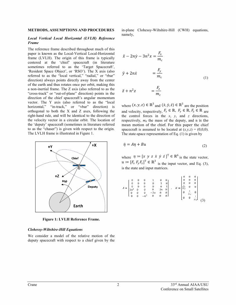
Local Vertical Local Horizontal (LVLH) Reference Frame The reference frame described throughout much of this paper is known as the Local-Vertical Local-Horizontal frame (LVLH). The origin of this frame is typically centered at the ‘chief’ spacecraft (in literature sometimes referred to as the ‘Target Spacecraft’, ‘Resident Space Object’, or ‘RSO’). The X axis (also referred to as the “local vertical,” “radial,” or “rbar” direction) always points directly away from the center of the earth and thus rotates once per orbit, making this a non-inertial frame. The Z axis (also referred to as the “cross-track” or “out-of-plane” direction) points in the direction of the chief spacecraft’s angular momentum vector. The Y axis (also referred to as the “local horizontal,” “in-track,” or “vbar” direction) is orthogonal to both the X and Z axes, following the right-hand rule, and will be identical to the direction of the velocity vector in a circular orbit. The location of the ‘deputy’ spacecraft (sometimes in literature referred to as the “chaser”) is given with respect to the origin. The LVLH frame is illustrated in Figure 1.

Figure 1: LVLH Reference Frame.

Clohessy-Wiltshire-Hill Equations We consider a model of the relative motion of the deputy spacecraft with respect to a chief given by the

in-plane Clohessy-Wiltshire-Hill (CWH) equations, namely,

�̈�𝑥 − 2𝑛𝑛�̇�𝑦 − 3𝑛𝑛2𝑥𝑥 =𝐹𝐹𝑥𝑥𝑚𝑚𝑐𝑐

�̈�𝑦 + 2𝑛𝑛�̇�𝑥 =𝐹𝐹𝑦𝑦𝑚𝑚𝑐𝑐

(1)

�̈�𝑧 + 𝑛𝑛2𝑧𝑧 =𝐹𝐹𝑧𝑧𝑚𝑚𝑐𝑐

where (𝑥𝑥, 𝑦𝑦, 𝑧𝑧) ∈ ℝ3 and (�̇�𝑥, �̇�𝑦, �̇�𝑧) ∈ ℝ3 are the position and velocity, respectively, 𝐹𝐹𝑥𝑥 ∈ ℝ, 𝐹𝐹𝑦𝑦 ∈ ℝ, 𝐹𝐹𝑧𝑧 ∈ ℝ are the control forces in the x, y, and z directions, respectively, md the mass of the deputy, and n is the mean motion of the chief. For this paper the chief spacecraft is assumed to be located at (x,y,z) = (0,0,0). The state-space representation of Eq. (1) is given by

�̇�𝜂 = 𝐴𝐴𝜂𝜂 + 𝐵𝐵𝐵𝐵 (2)

where 𝜂𝜂 ≔ [𝑥𝑥 𝑦𝑦 𝑧𝑧 𝑥𝑥 ̇ 𝑦𝑦 ̇ 𝑧𝑧 ̇ ]Τ ∈ ℝ6 is the state vector, 𝐵𝐵 ≔ [𝐹𝐹𝑥𝑥 𝐹𝐹𝑦𝑦𝐹𝐹𝑧𝑧]Τ ∈ ℝ3 is the input vector, and Eq. (3), is the state and input matrices.

(3)


Stochastic Reachability V&V Problem Outline Most of the algorithms employed were derived by Vinod et. al. [1], which proposes a scalable method for forward stochastic reachability analysis for uncontrolled linear systems with affine disturbance. The method uses Fourier transforms to efficiently compute the forward stochastic reach probability measure (FSRPM) and the forward stochastic reach (FSR) set. The method is applicable to systems with bounded or unbounded disturbance sets. While traditional approaches provide approximations, the method used here provides exact analytical expressions for the densities and probability of reaching the target set for linear time invariant (LTI) systems.

Reachability analysis of discrete-time dynamical systems with stochastic disturbance input is an established tool to provide probabilistic assurances of safety or performance and has been applied in several domains, including motion planning in robotics [2,3], spacecraft docking [4], fishery management and mathematical finance [5], and autonomous surveillance [6]. The computation of stochastic reachable and viable sets has been formulated within a dynamic programming framework [7], that generalizes to discrete-time stochastic hybrid systems, and suffers from the well-known curse of dimensionality [8].

A scalable method is presented to perform forward stochastic reachability analysis of LTI systems with stochastic dynamics, that is, a method to compute the FSR set as well as its FSRPM. It is shown that Fourier transforms can be used to provide exact reachability analysis, for systems with bounded or unbounded disturbances. The authors in Ref. [1] provides analytical expressions for the probability density and shows that explicit expressions can be derived in some cases.

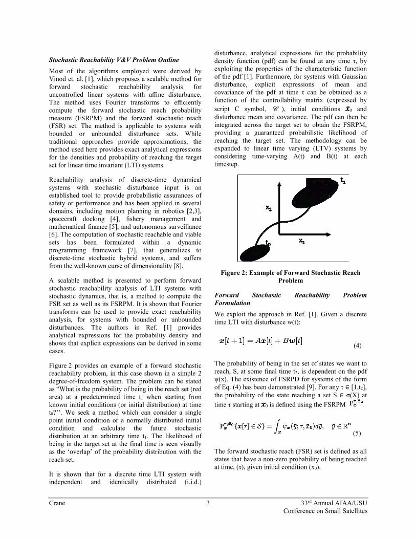
Figure 2 provides an example of a forward stochastic reachability problem, in this case shown in a simple 2 degree-of-freedom system. The problem can be stated as “What is the probability of being in the reach set (red area) at a predetermined time t1 when starting from known initial conditions (or initial distribution) at time t0?’’. We seek a method which can consider a single point initial condition or a normally distributed initial condition and calculate the future stochastic distribution at an arbitrary time t1. The likelihood of being in the target set at the final time is seen visually as the ‘overlap’ of the probability distribution with the reach set.

It is shown that for a discrete time LTI system with independent and identically distributed (i.i.d.)

disturbance, analytical expressions for the probability density function (pdf) can be found at any time τ, by exploiting the properties of the characteristic function of the pdf [1]. Furthermore, for systems with Gaussian disturbance, explicit expressions of mean and covariance of the pdf at time τ can be obtained as a function of the controllability matrix (expressed by script C symbol, C ), initial conditions 0 and disturbance mean and covariance. The pdf can then be integrated across the target set to obtain the FSRPM, providing a guaranteed probabilistic likelihood of reaching the target set. The methodology can be expanded to linear time varying (LTV) systems by considering time-varying A(t) and B(t) at each timestep.

Figure 2: Example of Forward Stochastic Reach Problem

Forward Stochastic Reachability Problem Formulation We exploit the approach in Ref. [1]. Given a discrete time LTI with disturbance w(t):

(4)

The probability of being in the set of states we want to reach, S, at some final time t2, is dependent on the pdf ψ(x). The existence of FSRPD for systems of the form of Eq. (4) has been demonstrated [9]. For any τ ∈ [1,t2], the probability of the state reaching a set S ∈ σ(X) at time τ starting at 0 is defined using the FSRPM .

(5)

The forward stochastic reach (FSR) set is defined as all states that have a non-zero probability of being reached at time, (τ), given initial condition (x0).


(6) (4)

For any time instant τ = [1,T] and an initial state x0, the pdf ψx(.,τ,x0) of Eq. (6) is given by:

(7)

(8)

is the inverse Fourier transform and where

(9)

is the controllability matrix. If we are given A, B, 𝜇𝜇𝑤𝑤�� , we can solve for 𝜇𝜇𝜏𝜏�� and Στ. These can in turn be used to solve for ΨW by;

(10)

this can then be fed into Eq. (7), the result of which is fed into Eq. (8), which is the FSRPD ψ(x). This result is fed into Eq. (11) to solve for the probability of being in the reach set at time τ.

(11)

Application to Systems with Gaussian Disturbance

It is further shown in Ref. [1] that when the disturbance w is Gaussian, the state trajectory of the LTI system with initial condition �̅�𝑥 0 and noise process w ~ N(μ, Σ)

P follows a Gaussian distribution of the form

(12)

Where τ = [1,T] and

(13)

(14)

The operation builds out a matrix of a size that is linearly dependent on the number of timesteps, τ. Note ⊗ is the tensor product. Finding the mean and covariance of a Gaussian distribution fully describes the probability density function at time τ and with initial condition �̅�𝑥 0 by:

(15)

Software-In-The-Loop (SITL) Simulation Environment A forward stochastic reachability toolbox (FSR toolbox) was developed in Matlab programming environment [1]. The V&V FSR toolbox results were compared with Monte Carlos run in a high-fidelity SITL simulation environment. The SITL testbed uses the L3 ADS Spacecraft Design Tool (SDT) to provide a faster-than-real-time, 6 degree-of-freedom dynamic model of the spacecraft including relevant orbital perturbations, physical environment effects, and individual hardware and software components. L3 ADS uses SDT-SITL to test the GNC FSW in a faster-than-real-time flight-representative environment, where realistic messaging interfaces are used to interact with the system, and other spacecraft subsystems are emulated by SDT, including sensor components and actuators. Starting with the same initial conditions scenarios were run in SDT-SITL using the FSW implementation of previously developed Hybrid Control Code (HCC).

RESULTS AND DISCUSSION The FSR code was initially compared to a Matlab Monte Carlo simulation in order to validate the overall approach for solving the reach avoid RPOD problem using a simplified dynamics model and spacecraft architecture. The complexity of the model was increased and tested.

Controlled LTI system with Gaussian Disturbance A known disturbance was added to the FSR toolbox with a linear quadratic regulator (LQR-1) controller. A corresponding simulation was set up in the Matlab


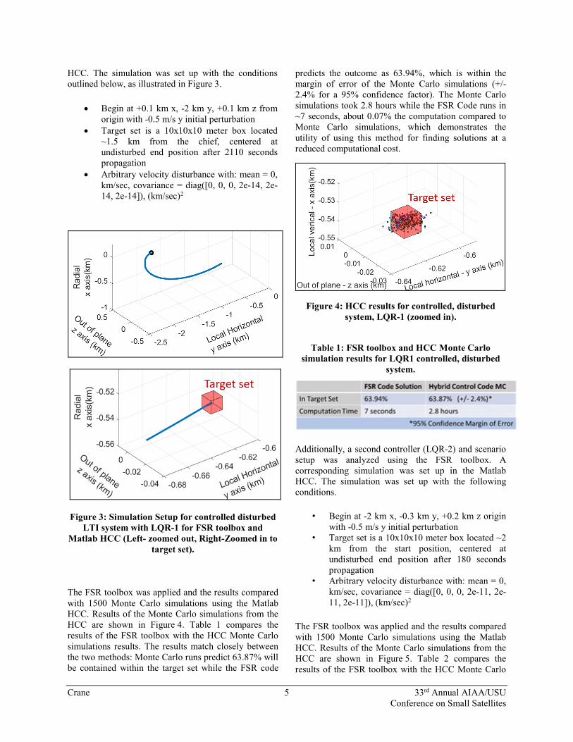
HCC. The simulation was set up with the conditions outlined below, as illustrated in Figure 3.

• Begin at +0.1 km x, -2 km y, +0.1 km z from origin with -0.5 m/s y initial perturbation

• Target set is a 10x10x10 meter box located ~1.5 km from the chief, centered at undisturbed end position after 2110 seconds propagation

• Arbitrary velocity disturbance with: mean = 0, km/sec, covariance = diag([0, 0, 0, 2e-14, 2e-14, 2e-14]), (km/sec)2

Figure 3: Simulation Setup for controlled disturbed LTI system with LQR-1 for FSR toolbox and

Matlab HCC (Left- zoomed out, Right-Zoomed in to target set).

The FSR toolbox was applied and the results compared with 1500 Monte Carlo simulations using the Matlab HCC. Results of the Monte Carlo simulations from the HCC are shown in Figure 4. Table 1 compares the results of the FSR toolbox with the HCC Monte Carlo simulations results. The results match closely between the two methods: Monte Carlo runs predict 63.87% will be contained within the target set while the FSR code

predicts the outcome as 63.94%, which is within the margin of error of the Monte Carlo simulations (+/-2.4% for a 95% confidence factor). The Monte Carlo simulations took 2.8 hours while the FSR Code runs in ~7 seconds, about 0.07% the computation compared to Monte Carlo simulations, which demonstrates the utility of using this method for finding solutions at a reduced computational cost.

Figure 4: HCC results for controlled, disturbed system, LQR-1 (zoomed in).

Table 1: FSR toolbox and HCC Monte Carlo

simulation results for LQR1 controlled, disturbed system.

Additionally, a second controller (LQR-2) and scenario setup was analyzed using the FSR toolbox. A corresponding simulation was set up in the Matlab HCC. The simulation was set up with the following conditions.

• Begin at -2 km x, -0.3 km y, +0.2 km z origin with -0.5 m/s y initial perturbation

• Target set is a 10x10x10 meter box located ~2 km from the start position, centered at undisturbed end position after 180 seconds propagation

• Arbitrary velocity disturbance with: mean = 0, km/sec, covariance = diag([0, 0, 0, 2e-11, 2e-11, 2e-11]), (km/sec)2

The FSR toolbox was applied and the results compared with 1500 Monte Carlo simulations using the Matlab HCC. Results of the Monte Carlo simulations from the HCC are shown in Figure 5. Table 2 compares the results of the FSR toolbox with the HCC Monte Carlo


simulations results. The results match closely between the two methods: Monte Carlo runs predict 66.73% will be contained within the target set while the FSR code predicts the outcome as 66.39%, which is within the margin of error of the Monte Carlo simulations (+/-2.4% for 95% confidence factor). Additionally, we can see that the Monte Carlo simulations took 18 minutes while the FSR Code runs in 0.3 seconds, about 0.03% the computation time. This again demonstrates the potential of using this method for finding solutions at a reduced computational cost.

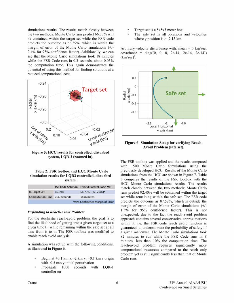
Figure 5: HCC results for controlled, disturbed system, LQR-2 (zoomed in).

Table 2: FSR toolbox and HCC Monte Carlo simulation results for LQR2 controlled, disturbed

system.

Expanding to Reach-Avoid Problem For the stochastic reach-avoid problem, the goal is to find the likelihood of getting into a given target set at a given time t1, while remaining within the safe set at all time from t0 to t1. The FSR toolbox was modified to enable reach avoid analysis.

A simulation was set up with the following conditions, as illustrated in Figure 6.

• Begin at +0.1 km x, -2 km y, +0.1 km z origin with -0.5 m/s y initial perturbation

• Propagate 1000 seconds with LQR-1 controller on

• Target set is a 5x5x5 meter box • The safe set is all locations and velocities

where y position is > -2.15 km.

Arbitrary velocity disturbance with: mean = 0 km/sec, covariance = diag([0, 0, 0, 2e-14, 2e-14, 2e-14]) (km/sec)2.

Figure 6: Simulation Setup for verifying Reach-Avoid Problem (safe set).

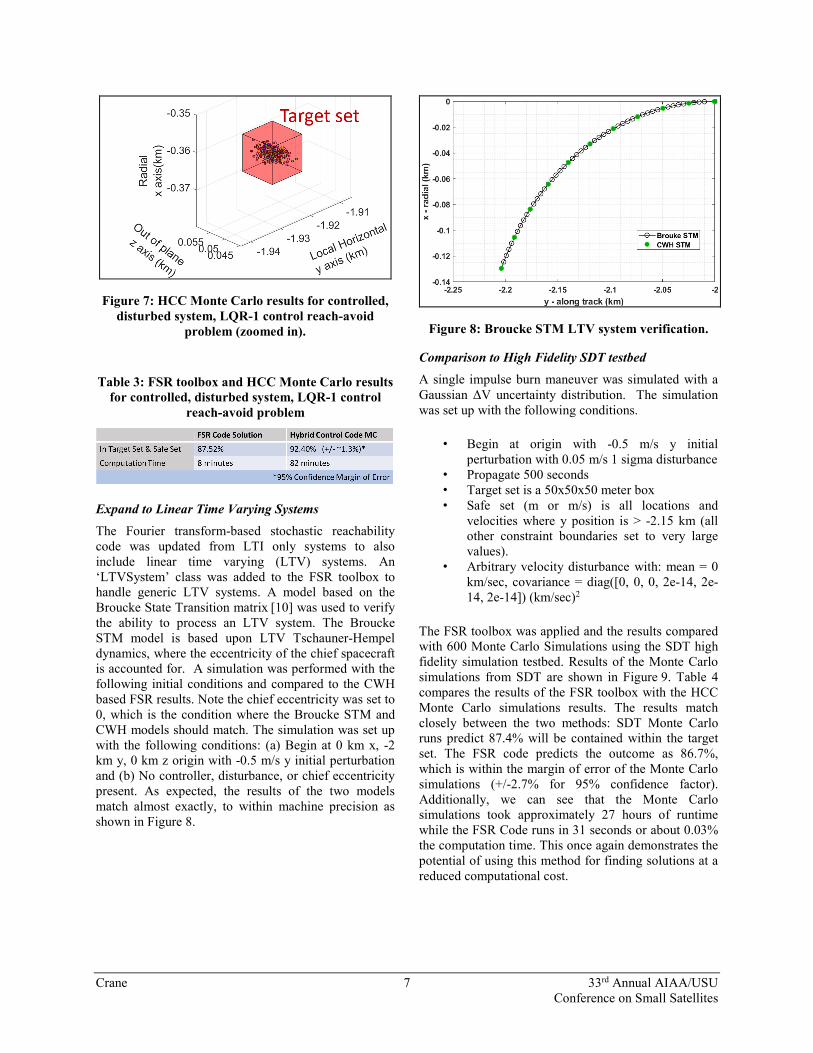
The FSR toolbox was applied and the results compared with 1500 Monte Carlo Simulations using the previously developed HCC. Results of the Monte Carlo simulations from the HCC are shown in Figure 7. Table 3 compares the results of the FSR toolbox with the HCC Monte Carlo simulations results. The results match closely between the two methods: Monte Carlo runs predict 92.40% will be contained within the target set while remaining within the safe set. The FSR code predicts the outcome as 87.52%, which is outside the margin of error of the Monte Carlo simulations (+/-1.3% for 95% confidence factor). This is not unexpected, due to the fact the reach-avoid problem approach contains several conservative approximations within it, i.e. the FSR code reach avoid function is guaranteed to underestimate the probability of safety of a given maneuver. The Monte Carlo simulations took 82 minutes to run while the FSR Code runs in 8 minutes, less than 10% the computation time. The reach-avoid problem requires significantly more computational resources compared to the reach only problem yet is still significantly less than that of Monte Carlo runs.


Figure 7: HCC Monte Carlo results for controlled, disturbed system, LQR-1 control reach-avoid

problem (zoomed in).

Table 3: FSR toolbox and HCC Monte Carlo results for controlled, disturbed system, LQR-1 control

reach-avoid problem

Expand to Linear Time Varying Systems The Fourier transform-based stochastic reachability code was updated from LTI only systems to also include linear time varying (LTV) systems. An ‘LTVSystem’ class was added to the FSR toolbox to handle generic LTV systems. A model based on the Broucke State Transition matrix [10] was used to verify the ability to process an LTV system. The Broucke STM model is based upon LTV Tschauner-Hempel dynamics, where the eccentricity of the chief spacecraft is accounted for. A simulation was performed with the following initial conditions and compared to the CWH based FSR results. Note the chief eccentricity was set to 0, which is the condition where the Broucke STM and CWH models should match. The simulation was set up with the following conditions: (a) Begin at 0 km x, -2 km y, 0 km z origin with -0.5 m/s y initial perturbation and (b) No controller, disturbance, or chief eccentricity present. As expected, the results of the two models match almost exactly, to within machine precision as shown in Figure 8.

Figure 8: Broucke STM LTV system verification.

Comparison to High Fidelity SDT testbed A single impulse burn maneuver was simulated with a Gaussian ΔV uncertainty distribution. The simulation was set up with the following conditions.

• Begin at origin with -0.5 m/s y initial perturbation with 0.05 m/s 1 sigma disturbance

• Propagate 500 seconds • Target set is a 50x50x50 meter box • Safe set (m or m/s) is all locations and

velocities where y position is > -2.15 km (all other constraint boundaries set to very large values).

• Arbitrary velocity disturbance with: mean = 0 km/sec, covariance = diag([0, 0, 0, 2e-14, 2e-14, 2e-14]) (km/sec)2

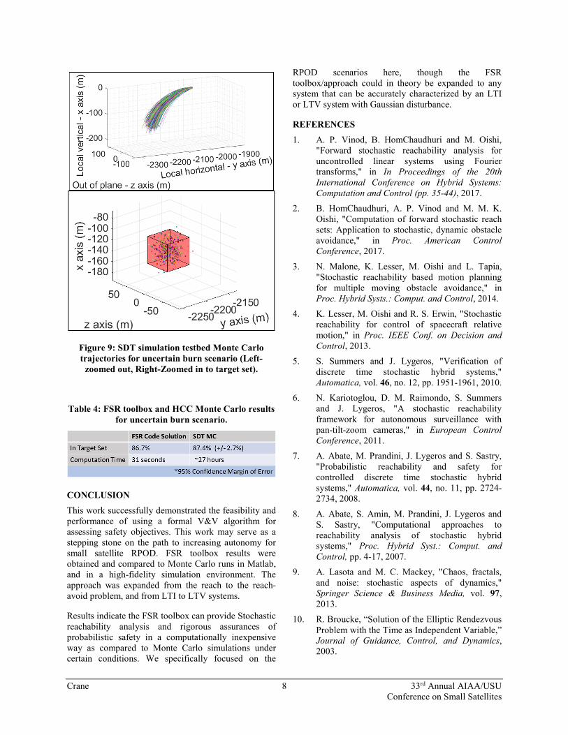
The FSR toolbox was applied and the results compared with 600 Monte Carlo Simulations using the SDT high fidelity simulation testbed. Results of the Monte Carlo simulations from SDT are shown in Figure 9. Table 4 compares the results of the FSR toolbox with the HCC Monte Carlo simulations results. The results match closely between the two methods: SDT Monte Carlo runs predict 87.4% will be contained within the target set. The FSR code predicts the outcome as 86.7%, which is within the margin of error of the Monte Carlo simulations (+/-2.7% for 95% confidence factor). Additionally, we can see that the Monte Carlo simulations took approximately 27 hours of runtime while the FSR Code runs in 31 seconds or about 0.03% the computation time. This once again demonstrates the potential of using this method for finding solutions at a reduced computational cost.


Figure 9: SDT simulation testbed Monte Carlo trajectories for uncertain burn scenario (Left-

zoomed out, Right-Zoomed in to target set).

Table 4: FSR toolbox and HCC Monte Carlo results for uncertain burn scenario.

CONCLUSION This work successfully demonstrated the feasibility and performance of using a formal V&V algorithm for assessing safety objectives. This work may serve as a stepping stone on the path to increasing autonomy for small satellite RPOD. FSR toolbox results were obtained and compared to Monte Carlo runs in Matlab, and in a high-fidelity simulation environment. The approach was expanded from the reach to the reach-avoid problem, and from LTI to LTV systems.

Results indicate the FSR toolbox can provide Stochastic reachability analysis and rigorous assurances of probabilistic safety in a computationally inexpensive way as compared to Monte Carlo simulations under certain conditions. We specifically focused on the

RPOD scenarios here, though the FSR toolbox/approach could in theory be expanded to any system that can be accurately characterized by an LTI or LTV system with Gaussian disturbance.

REFERENCES 1. A. P. Vinod, B. HomChaudhuri and M. Oishi,

"Forward stochastic reachability analysis for uncontrolled linear systems using Fourier transforms," in In Proceedings of the 20th International Conference on Hybrid Systems: Computation and Control (pp. 35-44), 2017.

2. B. HomChaudhuri, A. P. Vinod and M. M. K. Oishi, "Computation of forward stochastic reach sets: Application to stochastic, dynamic obstacle avoidance," in Proc. American Control Conference, 2017.

3. N. Malone, K. Lesser, M. Oishi and L. Tapia, "Stochastic reachability based motion planning for multiple moving obstacle avoidance," in Proc. Hybrid Systs.: Comput. and Control, 2014.

4. K. Lesser, M. Oishi and R. S. Erwin, "Stochastic reachability for control of spacecraft relative motion," in Proc. IEEE Conf. on Decision and Control, 2013.

5. S. Summers and J. Lygeros, "Verification of discrete time stochastic hybrid systems," Automatica, vol. 46, no. 12, pp. 1951-1961, 2010.

6. N. Kariotoglou, D. M. Raimondo, S. Summers and J. Lygeros, "A stochastic reachability framework for autonomous surveillance with pan-tilt-zoom cameras," in European Control Conference, 2011.

7. A. Abate, M. Prandini, J. Lygeros and S. Sastry, "Probabilistic reachability and safety for controlled discrete time stochastic hybrid systems," Automatica, vol. 44, no. 11, pp. 2724-2734, 2008.

8. A. Abate, S. Amin, M. Prandini, J. Lygeros and S. Sastry, "Computational approaches to reachability analysis of stochastic hybrid systems," Proc. Hybrid Syst.: Comput. and Control, pp. 4-17, 2007.

9. A. Lasota and M. C. Mackey, "Chaos, fractals, and noise: stochastic aspects of dynamics," Springer Science & Business Media, vol. 97, 2013.

10. R. Broucke, “Solution of the Elliptic Rendezvous Problem with the Time as Independent Variable,” Journal of Guidance, Control, and Dynamics, 2003.

Documents

A Formal Approach to Verification and Validation of