A formula for human retinal ganglion cell receptive fielddensity as a function of visual field location

Andrew B. Watson $NASA Ames Research Center, Moffett Field, CA, USA

In the human eye, all visual information must traversethe retinal ganglion cells. The most numerous subclass,the midget retinal ganglion cells, are believed to underliespatial pattern vision. Thus the density of their receptivefields imposes a fundamental limit on the spatialresolution of human vision. This density varies across theretina, declining rapidly with distance from the fovea.Modeling spatial vision of extended or peripheral targetsthus requires a quantitative description of midget celldensity throughout the visual field. Through an analysisof published data on human retinal topography of conesand ganglion cells, as well as analysis of prior formulas,we have developed a new formula for midget retinalganglion cell density as a function of position in themonocular or binocular visual field.

Introduction

The spatial resolution of human photopic vision islimited by optical blur, and beyond that by spatialsampling by retinal neurons. The initial sampling is bythe inner segments of the cone photoreceptors, andsubsequent resampling of their signals is performed, viavarious interneurons, by the retinal ganglion cells(RGC). These are the output cells of the human eye andconsequently their properties limit the signal that travelsto the rest of the brain. One class of these cells, themidget retinal ganglion cells (mRGC) are the mostnumerous; near the fovea they appear to sample a singlecone while in peripheral retina they gather signals frommultiple cones (Ahmad, Klug, Herr, Sterling, & Schein,2003; Dacey, 1993; Dacey & Petersen, 1992; Goodchild,Ghosh, &Martin, 1996; Kolb & Dekorver, 1991; Schein,1988). In consequence the mRGC likely set an upperbound on the spatial resolution of human vision,especially at low temporal frequencies (Hirsch & Curcio,1989; Merigan & Eskin, 1986; Merigan & Katz, 1990;Rossi & Roorda, 2010; Thibos, Cheney, &Walsh, 1987).

From a sampling point of view, the critical metric ofthe mRGC lattice is the local density or spacing ofadjacent mRGC receptive fields (mRGCf). Because this

spacing varies across the visual field, and because of itsfundamental role in modeling human visual spatialprocessing, it would be valuable to have a formula formRGCf spacing as a function of location in the visualfield.

An earlier formula for mRGCf density was devel-oped by Drasdo, Millican, Katholi, and Curcio (2007).While this formula was an important contribution, itwas largely based on psychophysical results (acuity vs.eccentricity). Since we would like to use our formula tomake psychophysical predictions, we sought to developa formula based only on anatomical data. Barten(1999) also produced a formula for RGC density alongan average meridian, but did not provide a derivationfor his result.

Dacey (1993) also provided a figure depictingestimated average midget ganglion cell density as afunction of eccentricity. However, his estimates arebased on highly variable estimates of dendritic field sizeand an assumption of unit coverage (the product ofdensity and field area) throughout the visual field. Also,separate estimates for the four meridians are notprovided. Nonetheless, we show in the Discussion thatour new formula is consistent with his empirical results.

The approach that we have taken is to seek a simpleanalytic formula that approximately satisfies known orprobable anatomical constraints.

Curcio, Sloan, Kalina, and Hendrickson (1990)measured the distribution of cone photoreceptors acrossthe retina in a set of eight human eyes. Consistent withearlier fragmentary reports (Osterberg, 1935), theyfound that density declined rapidly with eccentricity.They also described substantial meridional asymmetries,and large individual differences in peak density.

In a second paper six of those eyes, along with oneadditional eye, were used to measure the distribution ofretinal ganglion cells (Curcio & Allen, 1990). Thisdistribution also varies markedly with eccentricity, butunlike the cone distribution, it does not peak at thefovea. This is because in a central retinal zone theganglion cell bodies are displaced centrifugally somedistance from the inner segments of the cones to which

Citation: Watson, A. B. (2014). A formula for human retinal ganglion cell receptive field density as a function of visual fieldlocation. Journal of Vision, 14(7):15, 1–17, http://www.journalofvision.org/content/14/7/15, doi:10.1167/14.7.15.

Journal of Vision (2014) 14(7):15, 1–17 1http://www.journalofvision.org/content/14/7/15

doi: 10 .1167 /14 .7 .15 ISSN 1534-7362 ! 2014 ARVOReceived July 22, 2013; published June 30, 2014

they are connected through the bipolar cells, and thusfrom their receptive fields. This displacement zonecontinues up to eccentricities of around 138–178,depending on the meridian (Drasdo et al., 2007). Theextent of ganglion cell displacement as a function ofeccentricity of the cell body has been measured inprimate (Schein, 1988; Wassle, Grunert, Rohrenbeck,& Boycott, 1990) and human (Drasdo et al., 2007). Inhuman these displacements are as large as 2.28. As aresult, the peak RGC density occurs some 48–58 awayfrom the center of the fovea. Thus the local density ofthe cell bodies does not reflect the local density of theRGC receptive fields (RGCf).

However, the RGC distribution combined withseveral other constraints does allow a plausiblereconstruction of the distribution of RGCf. Theconstraints that we consider are:

1. Along a given meridian, the cumulative distributionof RGC and RGCf must agree outside thedisplacement zone.

2. In the fovea, it is likely that each cone connects (viabipolars) to exactly two mRGC (Kolb & Dekorver,1991).

3. Near the fovea midgets constitute most but not all ofthe ganglion cells. The ratio RGC/mRGC is given asabout 1.12 by Drasdo et al. (2007).

4. The hypothetical distribution of RGCf must beconsistent with the measured distribution of RGCoutside of the displacement zone.

Making use of these constraints, this report derives anew formula for RGC density as a function ofeccentricity along the four principal meridians, andmore generally of position on the retina or in the visualfield in degree coordinates.

The derivation relies on transformations from retinalcoordinates in mm to degree, based on a model eye(Drasdo & Fowler, 1974) and an assumed offset betweenoptical and visual axes (Charman, 1991), which aredescribed in Appendix 6. We also place in Appendix 5 anumber of formulas relating variousmetrics of points in ahexagonal sampling lattice, such as spacing, density, androw spacing. We also provide (see Appendix 2) with thisreport a supplementaryfileofMathematica functions thatimplement our formulas (Wolfram Research Inc., 2013).Lastly,weprovidea simple interactivedemonstration thatcomputes RGCf density and spacing at a selected visualfield location (see Appendix 1).

Conventions regarding meridians,locations, and the visual center

In retinal anatomy locations are often specified as adistance from a retinal center along one of the four

principal meridians. Because the topography is notradially symmetric, or even bilaterally symmetric,measurements differ along the four meridians. Thenaming of the meridians is a possible source ofconfusion, since different conventions are typically usedfor retinal anatomy and visual fields. Specifically, thenasal retina (the part nearest the nose) images thetemporal visual field (the part away from the nose), andvice versa, in both eyes. We avoid this confusion byalways referring to the visual field locations, even whendiscussing anatomy. We order the meridians temporal,superior, nasal, inferior, consistent with increasing polarangle in the visual field of the right eye, and assign themindexes of 1–4. When cartesian coordinates are used,positive x-coordinates refer to the temporal visual fieldof either eye, or the right binocular visual field.

A further possible confusion is that in the right eye,the temporal visual field is the right visual field, while inthe left eye, it is the left visual field. Thus when wecompute binocular visual fields, we combine thetemporal field of the right eye with the nasal field of theleft eye, and vice versa.

A final possible confusion is the definition of theretinal center. Remarkably, there appears to be noconsistent term for this concept. What we want is the‘‘visual center,’’ defined essentially as the intersection ofthe visual axis with the retina. It is not the same as the‘‘fovea’’ which is an area, not a point. It may wellcorrespond to the point of highest cone density, and isoperationally defined as the retinal location that imagesa fixated point, sometimes called the ‘‘preferred retinallocus of fixation’’ or PRLF (Rossi & Roorda, 2010).We will assume that anatomical measurements andvisual field locations are referenced to this commonvisual center.

Notation

In Appendix 3 we provide a more complete review ofnotation, but here we introduce some general conven-tions. The symbol r will indicate eccentricity in degree,d will indicate density in deg!2, and s will indicatespacing (of adjacent cells or receptive fields) in degrees.We use subscripts g, m, and c to denote RGC, mRGC,and cones respectively, and gf and mf to denote RGCand mRGC receptive fields. A particular meridian willbe indicated by an integer index k.

Cone densities

Curcio et al. (1990) measured cone photoreceptordensity across the retina in eight human eyes. Average

Journal of Vision (2014) 14(7):15, 1–17 Watson 2

data are provided in tables of cone densities in cones/mm2 in the four principal meridians at each of 34eccentricities in mm (Curcio, 2006). Using the conver-sion formulas described in Appendix 6, we haveconverted the densities to cones/deg2 as a function ofeccentricity in degree as shown in Figure 1. Writingdc(r, k) for the cone density at eccentricity r degreealong meridian k, we note that the foveal peak is dc(0,1)" dc(0)" 14,804.6. This peak density is plotted at theupper left on this log-log plot.

RGC densities

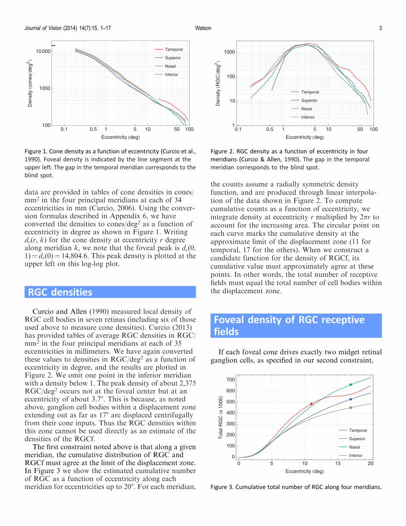
Curcio and Allen (1990) measured local density ofRGC cell bodies in seven retinas (including six of thoseused above to measure cone densities). Curcio (2013)has provided tables of average RGC densities in RGC/mm2 in the four principal meridians at each of 35eccentricities in millimeters. We have again convertedthese values to densities in RGC/deg2 as a function ofeccentricity in degree, and the results are plotted inFigure 2. We omit one point in the inferior meridianwith a density below 1. The peak density of about 2,375RGC/deg2 occurs not at the foveal center but at aneccentricity of about 3.78. This is because, as notedabove, ganglion cell bodies within a displacement zoneextending out as far as 178 are displaced centrifugallyfrom their cone inputs. Thus the RGC densities withinthis zone cannot be used directly as an estimate of thedensities of the RGCf.

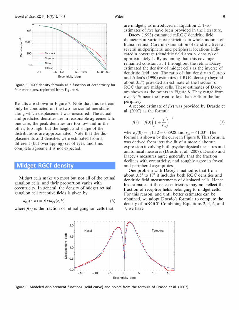
The first constraint noted above is that along a givenmeridian, the cumulative distribution of RGC andRGCf must agree at the limit of the displacement zone.In Figure 3 we show the estimated cumulative numberof RGC as a function of eccentricity along eachmeridian for eccentricities up to 208. For each meridian,

the counts assume a radially symmetric densityfunction, and are produced through linear interpola-tion of the data shown in Figure 2. To computecumulative counts as a function of eccentricity, weintegrate density at eccentricity r multiplied by 2pr toaccount for the increasing area. The circular point oneach curve marks the cumulative density at theapproximate limit of the displacement zone (11 fortemporal, 17 for the others). When we construct acandidate function for the density of RGCf, itscumulative value must approximately agree at thesepoints. In other words, the total number of receptivefields must equal the total number of cell bodies withinthe displacement zone.

Foveal density of RGC receptivefields

If each foveal cone drives exactly two midget retinalganglion cells, as specified in our second constraint,

Figure 1. Cone density as a function of eccentricity (Curcio et al.,1990). Foveal density is indicated by the line segment at theupper left. The gap in the temporal meridian corresponds to theblind spot.

Figure 2. RGC density as a function of eccentricity in fourmeridians (Curcio & Allen, 1990). The gap in the temporalmeridian corresponds to the blind spot.

Figure 3. Cumulative total number of RGC along four meridians.

Journal of Vision (2014) 14(7):15, 1–17 Watson 3

then the foveal density of midget retinal ganglion cellreceptive fields must be twice the cone density,

dmf #0$ " 2dc#0$: #1$

If midget cells constitute a fraction f(r) of allganglion cells at eccentricity r, then

dg f #0$ " f#0$!1dmf #0$

" 2f#0$!1dc#0$ #2$As noted below, f(0)!1 has been estimated as 1.12

(Drasdo et al., 2007) or 1.09 (Dacey, 1993). For reasonsoutlined below, here we adopt the value of 1.12, inwhich case dgf (0)" 2 · 1.12 · 14,804.6 " 33,163.2deg!2.

Density of RGC receptive fields

We now attempt to discover a function that willdescribe RGCf density as a function of eccentricity andsatisfy the constraints outlined in the Introduction. Foreach candidate function, we optimized the severalparameters with respect to an error function consistingof the sum of the squared errors between empirical andcomputed log densities for eccentricities outside theexclusion zone, and the weighted squared log of theratio of empirical and computed cumulative countswithin the exclusion zone (see points in Figure 3). Thisensures a reasonable fit to peripheral RGC densities,and to the cumulative counts. We used log densities inthe fit to accommodate the very wide range of densities,and to avoid giving the larger densities undue influencein the fit. We explored a wide range of functions,leading to the best-fitting one described below.

Since the work of Aubert and Foerster (1857) it hasbeen observed that many measures of visual resolutiondecline in an approximately linear fashion witheccentricity, at least up to the eccentricity of the blindspot (Strasburger, Rentschler, & Juttner, 2011). Be-cause resolution may depend on receptive field spacing,and since density is proportional to the inverse ofspacing squared (see Appendix 5), this suggests thatdensity might vary with eccentricity as

dg f #r$ " dg f #0$ 1% r

r2

! "!2

#3$

where dgf (0) is the density at r " 0, and r2 is theeccentricity at which density is reduced by a factor offour (and spacing is doubled). By itself, this did notprovide a good fit, especially at larger eccentricities.However we found that a simple modification, theaddition of an exponential, yielded an acceptable fit.The new function is given by

dg f#r; k$ " dg f #0$

· ak 1% r

r2;k

! "!2

%#1! ak$exp ! r

re;k

! "" #

#4$where ak is the weighting of the first term, and re,k is thescale factor of the exponential. The meridian isindicated by the index k. We have fit this expressionseparately for each meridian and optimized parametersrelative to the error function described above. Theresults are shown in Figure 4. For each meridian, weshow the average RGC densities reported by Curcioand Allen (1990), along with the fitted function. Thevertical gray line in each figure shows the assumed limitof the displacement zone. Note that only data pointsoutside the displacement zone are used in the fit. Theestimated parameters, predicted cell counts, and fittingerror are given in Table 1.

The fits are good for three of the four meridians.Both the peripheral densities and the cumulative countsare in close agreement. The agreement is less good forthe inferior meridian, largely due to the unusualdistribution of the far peripheral densities. Theanomalous bump at around 608 and subsequent rapiddecline are difficult to fit with simple analytic functions.For comparison, in Figure 5 we show the RGCf densityformula in the four meridians, replotted from Figure 4.

RGC displacement

One test of our formula for the density of RGCf is tocompare the predicted density of RGC within thedisplacement zone with the actual densities measuredby Curcio and Allen (1990). To generate thesepredictions we make use of measured displacementsfrom cone inner segment to retinal ganglion cell body insix human retinas along the horizontal meridian(Drasdo et al., 2007). For the separate nasal andtemporal meridians, they provided a mathematicalformula to describe the average displacement as afunction of RGC eccentricity. This can be converted toa function of cone inner segment eccentricity. Adifficulty with this function is that it does not providethe correct result at an eccentricity of zero. It shouldindicate the displacement corresponding to the RGCclosest to the fovea, but instead yields a value of 0.Rather than use their formula directly, we have insteadconstructed a new formula to describe displacement asa function of cone inner segment eccentricity. Weconstructed this new function to be a reasonable fit tothe function of Drasdo but to also yield a displacementof h(0) . 08 at 08 eccentricity. There is somedisagreement about the value of h(0). Drasdo stated

Journal of Vision (2014) 14(7):15, 1–17 Watson 4

that the first RGC are located 0.15 to 0.2 mm (0.538–0.718), whereas Curcio provides nonzero RGC densitiesat eccentricities as small as about 0.28 (see Figure 2).We have assumed a value of 0.58, but a value of 0.3gives very similar results.

The displacement function we used is the probabilitydensity function of the generalized Gamma distribution(multiplied by the gain d), given by

h#r$ " dce!

r!lb# $

cr!lb

# $ac!1

bC#a$: #5$

We attach no particular significance to the functionor its parameters. It serves only as a device to displace

hypothetical RGC cell bodies, as will be discussedbelow. This new function is shown in Figure 6, alongwith the corresponding functions provided by Drasdofor the two meridians. The parameters are provided inTable 2. Note that only three of the parameters areindependent, the other two are constrained by the valueof h(0) and by the peak value, which we set to themaximum of the fitted values.

Next we generated a population of RGC witheccentricities based on our density formula (Equation4). Eccentricities were random within annuli of 0.058.We then displaced each RGC centrifugally according tothe displacement function (Equation 5, Figure 6). Thedensity of the displaced cells was then computed.

Figure 4. Ganglion cell density as a function of eccentricity in four meridians. Data points are from Curcio and Allen (1990). The solidcurve is the fit of Equation 4 to the points outside the displacement zone. The dashed gray line indicates the approximate limit of thedisplacement zone. The density at eccentricity of zero is indicated by the line segment at the upper left.

Meridian k a r2 re

Data count(· 1000)

Model count(· 1000) Error rz

Temporal 1 0.9851 1.058 22.14 485.1 485.7 0.23 11Superior 2 0.9935 1.035 16.35 526.1 528.9 0.12 17Nasal 3 0.9729 1.084 7.633 660.9 661.1 0.01 17Inferior 4 0.996 0.9932 12.13 449.3 452.1 0.93 17

Table 1. Parameters and error for fits of Equation 4 in four meridians. Note: Also shown are measured and predicted cumulativecounts along each meridian within the displacement zone. The next-to-last column shows the fitting error outside the displacementzone. The last column indicates the assumed limit of the displacement zone.

Journal of Vision (2014) 14(7):15, 1–17 Watson 5

Results are shown in Figure 7. Note that this test canonly be conducted on the two horizontal meridiansalong which displacement was measured. The actualand predicted densities are in reasonable agreement. Inone case, the peak densities are too low and in theother, too high, but the height and shape of thedistributions are approximated. Note that the dis-placements and densities were estimated from adifferent (but overlapping) set of eyes, and thuscomplete agreement is not expected.

Midget RGCf density

Midget cells make up most but not all of the retinalganglion cells, and their proportion varies witheccentricity. In general, the density of midget retinalganglion cell receptive fields is given by

dmf#r; k$ " f#r$dg f#r; k$ #6$

where f(r) is the fraction of retinal ganglion cells that

are midgets, as introduced in Equation 2. Twoestimates of f(r) have been provided in the literature.

Dacey (1993) estimated mRGC dendritic fielddiameters at various eccentricities in whole mounts ofhuman retina. Careful examination of dendritic trees atseveral midperipheral and peripheral locations indi-cated a coverage (dendritic field area · density) ofapproximately 1. By assuming that this coverageremained constant at 1 throughout the retina Daceyestimated the density of midget cells as the inverse ofdendritic field area. The ratio of that density to Curcioand Allen’s (1990) estimates of RGC density (beyondabout 3.58) provided an estimate of the fraction ofRGC that are midget cells. These estimates of Daceyare shown as the points in Figure 8. They range fromover 95% near the fovea to less than 50% in the farperiphery.

A second estimate of f(r) was provided by Drasdo etal. (2007) as the formula

f#r$ " f#0$ 1% r

rm

! "!1

#7$

where f(0) " 1/1.12 " 0.8928 and rm " 41.038. Theformula is shown by the curve in Figure 8. This formulawas derived from iterative fit of a more elaborateexpression involving both psychophysical measures andanatomical measures (Drasdo et al., 2007). Drasdo andDacey’s measures agree generally that the fractiondeclines with eccentricity, and roughly agree in fovealand peripheral asymptotes.

One problem with Dacey’s method is that fromabout 3.58 to 178 it includes both RGC densities anddendritic field measurements of displaced cells. Hencehis estimates at those eccentricities may not reflect thefraction of receptive fields belonging to midget cells.For this reason, and until better estimates can beobtained, we adopt Drasdo’s formula to compute thedensity of mRGCf. Combining Equations 2, 4, 6, and7, we have

Figure 6. Modeled displacement functions (solid curve) and points from the formula of Drasdo et al. (2007).

Figure 5. RGCf density formula as a function of eccentricity forfour meridians, replotted from Figure 4.

Journal of Vision (2014) 14(7):15, 1–17 Watson 6

dmf#r; k$ " 2dc#0$ 1% r

rm

! "!1

· ak 1% r

r2;k

! "!2

%#1! ak$exp ! r

re;k

! "" #

:

#8$

This formula is plotted in Figure 9 for the fourmeridians.

mRGCf spacing

On the assumption of hexagonal packing (EquationA4), the spacing of adjacent midget receptive fields isgiven by

smf#r; k$ "%%%%%%%%%%%%%%%%%%%%%%%

2%%%3p

dmf#r; k$

s: #9$

Spacing at a binocular horizontal eccentricity can becomputed by averaging densities at correspondingeccentricities in temporal and nasal meridians andconverting to spacing. We can also compute the‘‘mean’’ spacing, the average of all four meridians, byaveraging densities and converting to spacing. Theseformulas for spacing are plotted in Figure 10. We showthe individual meridians and the ‘‘Horizontal’’ and‘‘Mean’’ versions.

Note that the midget RGC are composed ofapproximately equal numbers of ‘‘on’’ and ‘‘off’’ centercells (we neglect reports of asymmetry between the two

types). Typically we are concerned with the spacingwithin one class, in which case density is halved and thespacings should be multiplied by =2. In Figure 11 weshow the formula scaled in this way for eccentricitiesbetween 08 and 108, and we express the spacings inarcmin.

Averaged across meridians, the computed spacing ofmRGCf is very nearly linear (R2" 0.9997). This allowsus to write the following simple approximation foraverage spacing in either on- or off-center mosaic,where both s and r are expressed in degrees.

60s " 0:53% 0:434r #10$

This convenient result is the due to the form ofEquation 4, and the fact that the second exponentialterm does not have much effect for eccentricities lessthan 308.

Extension to arbitrary retinallocations

To this point we have developed formulas describingspacing as a function of eccentricity along each of thefour principal meridians. We would like to extend theseformulas to describe spacing at an arbitrary point {x,y} in the retina. To do this we make the assumptionthat within any one quadrant of the retina the iso-spacing contours are ellipses. This is consistent with theidea that spacing changes smoothly with the angle of aray extending from the visual center. An example isshown in Figure 12. The eccentricities at the intersec-tions of the ellipse with the two enclosing meridians arerx and ry.

Under the ellipse assumption, we can write

x

rx

! "2

% y

ry

! "2

" 1 #11$

Meridian a "b(deg) c d l(deg)

Temporal 1.8938 2.4598 0.91565 14.904 !0.09386Nasal 2.4607 1.7463 0.77754 15.111 !0.15933

Table 2. Parameters of the displacement function (Equation 5and Figure 6).

Figure 7. Modeled and measured density of displaced retinal ganglion cells in temporal (left) and nasal (right) meridians.

Journal of Vision (2014) 14(7):15, 1–17 Watson 7

And because they are on an iso-spacing curve,

s#rx; 1$ " s#ry; 2$ #12$

Given numerical values for x and y, we can solveEquations 11 and 12 together to find numericalsolutions for rx and ry, and then we can compute

s# x; yf g$ " s#rx; 1$ #13$

To avoid solving a system of equations, we havefound that the following approximation works well.Let rxy be the radial eccentricity of the point {x, y},

rxy "%%%%%%%%%%%%%%%x2 % y2

p#14$

Then we compute

s# x; yf g$ "

%%%%%%%%%%%%%%%%%%%%%%%%%%%%%%%%%%%%%%%%%%%%%%%%%%%%%%%%%%%%%%%%%%x

rxys#rxy; 1$

! "2

% y

rxys#rxy; 2$

! "2s

" 1

rxy

%%%%%%%%%%%%%%%%%%%%%%%%%%%%%%%%%%%%%%%%%%%%%%%%%%x2s#rxy; 1$2 % y2s#rxy; 2$2

q#15$

This approximation is always within 1.7% of thevalue obtained by Equations 10 through 12. Equation15 is easily generalized to work for arbitrary retinalquadrants. Since the sign of the horizontal coordinateis arbitrary, we define positive x values to mean thetemporal visual field. This corresponds to the rightvisual field for the right eye, and the left visual field forthe left eye.

Extension to arbitrary binocularvisual field locations

Equation 15 computes mRGC spacing at locationsspecified in visual field coordinates in one eye. Inpsychophysical modeling of natural vision, it is usefulto compute spacing at locations specified in thebinocular visual field. To do this we compute thespacing at corresponding visual field locations in the

Figure 8. Estimated fraction of RGC that are midget cells as afunction of eccentricity.

Figure 9. mRGCf density formula as a function of eccentricity(Equation 8).

Figure 10. Formula for mRGCf spacing.

Figure 11. Formula for on or off mRGCf spacing for eccentricities08–108.

Journal of Vision (2014) 14(7):15, 1–17 Watson 8

two eyes, convert them to densities (Equation 2),compute their mean, and convert back to spacing(Equation A4). After simplifying, we obtain thefollowing result for binocular spacing sB:

sB# x; yf g$ "%%%2p

%%%%%%%%%%%%%%%%%%%%%%%%%%%%%%%%%%%%%%%%%%%%%%%%%s# !x; yf g$2s# x; yf g$2

s# !x; yf g$2 % s# x; yf g$2

s

: #16$

With this function we can compute a plot of theNyquist frequency over the binocular visual field, asshown in Figure 13. In this calculation we have dividedthe value by =2, based on the assumption ofoverlapping lattices of on- and off-center cells. Thepeak value is 65.4 cycles/deg. Because there is someambiguity about the best way to combine the densitiesof the two eyes, in our supplementary materials we alsoprovide functions that compute the maximum density,or the total density of the two eyes.

Discussion

Ratio of midget RGC and cones

In Figure 14 we plot the ratio between mRGCfdensities computed from Equation 8 and cone densitiesreported by Curcio et al. (1990). Although we did notimpose this as a constraint in estimating a function forthe density of ganglion cells, the ratio remains close to 2for the central several degrees. This is roughlyconsistent with Dacey’s report that up to about 48mRGC dendritic fields remain at a minimum sizeappropriate to connection with a single bipolar, andthereby to a single cone. Beyond about 68, he foundthat dendritic fields enlarge and begin to show clusterssuggesting input from multiple cones, and consistentwith the decline in the ratio in Figure 14. Our result isalso consistent with Schein’s estimate that the ratioremains constant out to about 2.58 in primates (Schein,1988).

Comparison with Drasdo et al. (2007)

In Figure 15 we compare mRGCF spacing computedfrom our formula to densities computed from theformula of Drasdo et al. (2007), converted to spacingsby Equation A4. While there is considerable agreement,there are some significant discrepancies. In particularthe curves for the superior and inferior meridians arenearly interchanged in the two formulas. Our formulais consistent with Curcio and Allen (1990) who clearlyshow higher density (smaller spacing) in superior versusinferior meridians beyond about 68 (see Figure 2), while

Figure 12. A hypothetical iso-spacing curve in one quadrant,including a point {x, y} and points on the two enclosingmeridians.

Figure 13. Nyquist frequency over the binocular visual field based on the density formula and assuming separate and equal on- andoff-center populations.

Journal of Vision (2014) 14(7):15, 1–17 Watson 9

Drasdo’s formula shows the opposite, for unknownreasons. We also note that the Drasdo formula isdefined only up to 308, while ours extends at least as faras 908.

Comparison with dendritic field diameter

Dacey measured dendritic field diameters of midgetganglion cells in human retina (Dacey, 1993; Dacey &Petersen, 1992). In Figure 16 we have reproduced hisFigure 4B, that shows diameter as a function ofeccentricity. The filled points are for the temporalquadrant, open points are for the other quadrants.Near the fovea, where mRGC connect to single cone,we do not expect any relationship between fielddiameter and cell spacing. However in the periphery,Dacey found that within either the on- or off-centerlattice, spacing and diameter were about equal. Thisallows us to compare his measures of diameter to ourspacing formula for equivalent eccentricities andquadrants. Formula values for the temporal meridianand the mean of the other three meridians are shown by

the colored curves in Figure 16. The computed spacingis for either the on- or off-center lattice. The agreementis reasonable, especially considering the sizable scatterin measurements of diameter.

Comparison with acuity

Rossi and Roorda (2010) provide estimates of letteracuity, expressed as minimum angle of resolution(MAR) for five observers viewing targets underadaptive optics conditions. The targets were at nasalvisual field locations between 08 and 2.58. In Figure 17we compare their results with the computed rowspacing, assuming separate on- and off-cell lattices. Weuse separate lattices on the assumption that, at leastnear the fovea, both an on and an off midget cell arerequired to signal the signed value of local contrast. In

Figure 15. Comparison of formulas of Watson and Drasdo et al.(2007) (dashed).

Figure 16. Dendritic field diameter as a function of eccentricityfor human mRGC as measured by Dacey (1993). Filled pointsare for the temporal meridian; open points are for otherquadrants. Gray curve is Dacey’s estimate of the mean. Red andblue curves show spacing calculated from our formula for thetemporal meridian or the mean of the other meridians.

Figure 17. Human letter acuity (points) along the nasal meridianof five observers from Rossi and Roorda (2010) and row spacingfrom our formula for the same meridian (line).

Figure 14. Ratio of mRGCf to cones as a function of eccentricitybased on the Watson formula for mRGCf density.

Journal of Vision (2014) 14(7):15, 1–17 Watson 10

addition, where each cone drives one on and one offmidget, we know the two midgets have the samereceptive field location. Specifically, the functionreturned by Equation 9 is multiplied by 60 =2 =3 / 2"30 =6 to reflect the halved density, conversion to rowspacing, and conversion to arcmin. The agreement isexcellent. This is not surprising, since Rossi andRoorda previously showed good agreement with theformula of Drasdo et al. (2007), to which ours is similarfor small eccentricities.

Estimates of peripheral acuity are complicated by thepossibility of aliasing. Anderson, Mullen, and Hess(1991) attempted to bypass this problem by usingdirection discrimination of drifting gratings. Theirresults are plotted in Figure 18, along with calculationsof Nyquist frequency of the on- or off-center mRGCflattice from Equations 8 and A3. The agreement isreasonable. One caveat regarding the comparison at r"0 is that these data were collected with Gabor targetsthat extended (at half height) well over 0.58, so thatperformance may reflect the averaging spacing overthat area. The precise relationship between mRGCfspacing and acuity is beyond the scope of this paper(Anderson & Thibos, 1999), here we only point to thegeneral agreement in both the shape and absolute levelof the calculations.

Comparison with Sjostrand

In a series of papers Sjostrand, Popovic, andcolleagues measured human RGC densities at eccen-tricities from about 28 to 348 eccentricity along thevertical meridian in sectioned human retinas (Popovic& Sjostrand, 2001, 2005; Sjostrand, Olsson, Popovic,& Conradi, 1999; Sjostrand, Popovic, Conradi, &Marshall, 1999). From these densities, using their ownestimates of displacement, the inferred RGC spacingat various eccentricities. Their formula for conversion

from density to spacing actually yields the row spacing(Equation A1) not the spacing between cells (EquationA4), which is 2 / =3 larger. Even taking this intoaccount, their values are about a factor 0.75 smallerthan those computed from our formula for the meanof superior and inferior meridians. However theirvalues are also discrepant with Drasdo’s formula(Figure 6) and with spacing estimated from Dacey’sestimates of mRGC field diameter (Figure 16). Somepart of this discrepancy may arise from their formulafor displacement, which though similar in form is onlyhalf the magnitude of ours or that of Drasdo, who hasalso commented on this discrepancy (Drasdo et al.,2007).

Popovic and Sjostrand (2005) measured acuity ofthree observers at eccentricities between 5.88 and 26.48in both eyes, one of which was subsequently enucle-ated. Ganglion cell densities and spacings weremeasured along the vertical meridian. Acuity (MAR)was measured using high-pass resolution perimetry.They found MAR was approximately proportional toRGC spacing over the full range of eccentricities. Theconstant of proportionality was rather large (4.24),especially compared to the value of 1 we have used inFigures 17 and 18. They note that correcting for thelow contrast of their target (0.25), and consideringonly spacing in one class (on or off) of midget cells aswe have done, would lower the constant to 1.43. Theremaining discrepancy may be due to their lowestimates of spacing, as noted above. In general, theirresults support the notion that psychophysical reso-lution is governed by the mRGC spacing.

Midget fraction

Perhaps the least secure element of our formula is themidget fraction, the function describing the fraction ofall ganglion cells that are midget as a function ofeccentricity. As noted above (Figure 8) there arediscrepancies between available estimates. We haveadopted the formula of Drasdo, but it is unclearwhether that is accurate, especially at very largeeccentricities, where it continues to descend to values aslow as 0.25. In the periphery, where his estimates arearguably most accurate, Dacey’s estimates appear thelevel off at about 0.5. Until more definitive estimatesare available, we will have to acknowledge thespeculative nature of this element.

Variability

I have based my formula on average densities ofcones and retinal ganglion cells (Curcio & Allen,

Figure 18. Human grating acuity (points) from Anderson et al.(1991) and calculated Nyquist frequency of midget RGC.

Journal of Vision (2014) 14(7):15, 1–17 Watson 11

1990; Curcio et al., 1990). Curcio et al. (1990) note avery large variation in peak cone density in their setof nine eyes, ranging from 98,200 to 324,100 mm!2

(7,385 to 24,372 deg!2) (coefficient of variation;0.46). When two anomalous eyes are excluded, thelower bound only increases to 166,000 mm!2 (12,483deg!2). This variation largely disappeared at eccen-tricities beyond 18, so that the total number of coneswithin a radius of about 3.68 (or over the entireretina) was nearly constant (coefficient of variation;0.1). However, more recent density estimates fromin vivo measurement show a fairly consistent coeffi-cient of variation (;0.2) regardless of eccentricity(Song, Chui, Zhong, Elsner, & Burns, 2011). Theselatter authors have also shown an up to 25%decrement in density with age, primarily at eccen-tricities less than 1.68. Curcio’s data, and ourformula, are consistent with the data for theiryounger group of observers.

Ganglion cell densities also show sizable individualdifferences (Curcio & Allen, 1990). However, perhapsin contrast to cones, the total number variesconsiderably, from 0.71 to 1.54 million cells over a setof six eyes. This variation seems to be consistentacross the retina. Variation at the fovea cannot bedirectly determined because of the displacement of theRGC.

Beyond these variations between individuals andwith respect to age, there may be additional sources ofvariability and measurement error. Thus while aformula for the average may be useful, it is importantto note that individuals may differ considerably fromthese computed values.

Conclusions

We have derived a mathematical formula for thedensity of receptive fields of human retinal ganglioncells as a function of position in the monocular orbinocular visual field. Densities can also be computedfor the receptive fields of the midget subclass ofganglion cells. Both spacing and position are expressedin degrees. The formula has several advantages overexisting formulas, which are based on psychophysics,limited to small eccentricities, confined to specificmeridians, or are inaccurate in the foveal region. Sincethe midget retinal ganglion cells provide the primarylimit on human visual spatial resolution across thevisual field, this formula may be useful in the modelingof human spatial vision.

Keywords: vision, perception, acuity, retinal topogra-phy, retinal ganglion cells, midget retinal ganglion cell,eccentricity, peripheral vision, visual resolution

Acknowledgments

I thank Albert Ahumada, Jeffrey Mulligan, DennisDacey, Heinz Wassle, Joy Hirsch, Neville Drasdo,Tony Movshon, and Denis Pelli and two anonymousreferees for comments on earlier versions of themanuscript. I thank Christine Curcio for providing thecone density and retinal ganglion cell data, and EthanRossi for providing the acuity data in Figure 17. Thiswork supported by the NASA Space Human FactorsResearch Project WBS 466199.

Commercial relationships: none.Corresponding author: Andrew B. Watson.Email: andrew.b.watson@nasa.gov.Address: NASA Ames Research Center, Moffett Field,CA, USA.

References

Ahmad, K. M., Klug, K., Herr, S., Sterling, P., &Schein, S. (2003). Cell density ratios in a fovealpatch in macaque retina. Visual Neuroscience,20(2), 189–209.

Anderson, R. S., & Thibos, L. N. (1999). Relationshipbetween acuity for gratings and for tumbling-Eletters in peripheral vision. Journal of the OpticalSociety of America A, 16(10), 2321–2333, http://josaa.osa.org/abstract.cfm?URI"josaa-16-10-2321.

Anderson, S. J., Mullen, K. T., & Hess, R. F. (1991).Human peripheral spatial resolution for achromaticand chromatic stimuli: Limits imposed by opticaland retinal factors. Journal of Physiology, 442, 47–64, http://www.ncbi.nlm.nih.gov/pubmed/1798037.

Aubert, H. R., & Foerster, C. F. R. (1857). Beitrage zurKenntniss des indirecten Sehens. (I). Untersuchun-gen uber den Raumsinn der Retina [Translation:Contributions to the knowledge of the indirectvision: I. Studies on the sense of space of the retina].Archiv fur Ophthalmologie, 3, 1–37.

Barten, P. G. J. (1999). Contrast sensitivity of the humaneye and its effects on image quality. Bellingham,WA: SPIE Optical Engineering Press.

Charman, W. N. (1991). Optics of the human eye. In J.Cronly Dillon (Ed.), Visual optics and instrumen-tation (pp. 1–26). Boca Raton: CRC Press.

Curcio, C. (2006). 4meridians.xls. Retrieved fromhttp://www.cis.uab.edu/sloan/PRtopo/4meridians.xls.

Curcio, C. (2013). Curcio_JCompNeurol1990_GCtopo_F6.xls.

Journal of Vision (2014) 14(7):15, 1–17 Watson 12

Curcio, C. A., & Allen, K. A. (1990). Topography ofganglion cells in human retina. Journal of Com-parative Neurology, 300(1), 5–25.

Curcio, C. A., Sloan, K. R., Kalina, R. E., &Hendrickson, A. E. (1990). Human photoreceptortopography. Journal of Comparative Neurology,292(4), 497–523, http://www.ncbi.nlm.nih.gov/pubmed/2324310.

Dacey, D. M. (1993). The mosaic of midget ganglioncells in the human retina. Journal of Neuroscience,13(12), 5334–5355, http://www.ncbi.nlm.nih.gov/pubmed/8254378.

Dacey, D. M., & Petersen, M. R. (1992). Dendritic fieldsize and morphology of midget and parasol ganglioncells of the human retina. Proceedings of the NationalAcademy of Sciences, USA, 89(20), 9666–9670, http://www.ncbi.nlm.nih.gov/pubmed/1409680.

Drasdo, N., & Fowler, C. W. (1974). Non-linearprojection of the retinal image in a wide-angleschematic eye. British Journal of Ophthalmology,58(8), 709–714, http://www.ncbi.nlm.nih.gov/pubmed/4433482.

Drasdo, N., Millican, C. L., Katholi, C. R., & Curcio,C. A. (2007). The length of Henle fibers in thehuman retina and a model of ganglion receptivefield density in the visual field. Vision Research,47(22), 2901–2911, http://www.ncbi.nlm.nih.gov/pubmed/17320143.

Emsley, H. H. (1952). Visual optics (5th ed.). London:Hatton Press.

Goodchild, A. K., Ghosh, K. K., & Martin, P. R.(1996). Comparison of photoreceptor spatial den-sity and ganglion cell morphology in the retina ofhuman, macaque monkey, cat, and the marmosetCallithrix jacchus. Journal of Comparative Neurol-ogy, 366(1), 55–75, http://www.ncbi.nlm.nih.gov/pubmed/8866846.

Hirsch, J., & Curcio, C. A. (1989). The spatialresolution capacity of human foveal retina. VisionResearch, 29(9), 1095–1101.

Kolb, H., & Dekorver, L. (1991). Midget ganglion cellsof the parafovea of the human retina: A study byelectron microscopy and serial section reconstruc-tions. Journal of Comparative Neurology, 303(4), 617–636, http://www.ncbi.nlm.nih.gov/pubmed/1707423.

Merigan, W. H., & Eskin, T. A. (1986). Spatio-temporal vision of macaques with severe loss of P-beta retinal ganglion cells. Vision Research, 26,1751–1761.

Merigan, W. H., & Katz, L. M. (1990). Spatialresolution across the macaque retina. VisionResearch, 30(7), 985–991.

Osterberg, G. A. (1935). Topography of the layer ofrods and cones in the human retina. Acta Oph-thalmologica, 6(Suppl. VI), 1–97.

Popovic, Z., & Sjostrand, J. (2005). The relationbetween resolution measurements and numbers ofretinal ganglion cells in the same human subjects.Vision Research, 45(17), 2331–2338.

Popovic, Z., & Sjostrand, J. (2001). Resolution,separation of retinal ganglion cells, and corticalmagnification in humans. Vision Research, 41(10),1313–1319.

Rossi, E. A., & Roorda, A. (2010). The relationshipbetween visual resolution and cone spacing in thehuman fovea. Nature Neuroscience, 13(2), 156–157,http://dx.doi.org/10.1038/nn.2465.

Schein, S. J. (1988). Anatomy of macaque fovea andspatial densities of neurons in foveal representa-tion. Journal of Comparative Neurology, 269(4),479–505, http://www.ncbi.nlm.nih.gov/pubmed/3372725.

Sjostrand, J., Olsson, V., Popovic, Z., & Conradi, N.(1999). Quantitative estimations of foveal andextra-foveal retinal circuitry in humans. VisionResearch, 39(18), 2987–2998.

Sjostrand, J., Popovic, Z., Conradi, N., & Marshall, J.(1999). Morphometric study of the displacement ofretinal ganglion cells subserving cones within thehuman fovea. Graefes Archives for Clinical &Experimental Ophthalmology, 237(12), 1014–1023.

Song, H., Chui, T. Y. P., Zhong, Z., Elsner, A. E., &Burns, S. A. (2011). Variation of cone photore-ceptor packing density with retinal eccentricity andage. Investigative Ophthalmology & Visual Science,52(10), 7376–7384, http://www.iovs.org/content/52/10/7376. [Pubmed] [Article]

Strasburger, H., Rentschler, I., & Juttner, M. (2011).Peripheral vision and pattern recognition: A review.Journal of Vision, 11(5):13, 1-82, http://www.journalofvision.org/content/11/5/13, doi:10.1167/11.5.13. [Pubmed] [Article]

Thibos, L., Cheney, F., & Walsh, D. (1987). Retinallimits to the detection and resolution of gratings.Journal of the Optical Society of America A, 4(8),1524–1529.

Wassle, H., Grunert, U., Rohrenbeck, J., & Boycott, B.B. (1990). Retinal ganglion cell density and corticalmagnification factor in the primate. Vision Re-search, 30(11), 1897–1911, http://www.ncbi.nlm.nih.gov/pubmed/2288097.

Wolfram Research Inc. (2013). Mathematica (Version9.0). Champaign, IL: Author.

Journal of Vision (2014) 14(7):15, 1–17 Watson 13

Appendix 1: Demonstration

As a supplement to this paper we provide aninteractive calculator that returns density and spacingat arbitrary visual field locations. The demonstrationrequires the use of the Wolfram CDF player, availableat https://www.wolfram.com/cdf-player/. An illustra-tion of the calculator is shown in Figure 19.

Appendix 2: Mathematica tablesand functions

As a supplement we provide aMathematicaNotebookthat contains a number of tables and functions derivedand used in this report. The Notebook is a text file, but ismost readable using the free Wolfram CDF Playeravailable at https://www.wolfram.com/cdf-player/.

Figure 19. Demonstration of Retinal Topography Calculator.

Journal of Vision (2014) 14(7):15, 1–17 Watson 14

Appendix 3: Notation

The following is a table of notation used in thisreport.

Appendix 4: Formula parametersand useful numbers

Appendix 5: Density, spacing, rowspacing, and Nyquist frequency

At least in the fovea, both photoreceptors andmidget ganglion cell receptive fields form an approx-imately hexagonal lattice. Because we will make use ofthese formulas in the text, we review here therelationships among various metrics of a hexagonallattice of points: S(deg)" the spacing between adjacentpoints, R(deg)" the spacing between rows of points,D(deg!2) " the density of points, and N(c/deg)" theNyquist frequency of the lattice (the highest frequencythat can be supported by a particular row spacing).These formulas will allow us to convert among thesemetrics. Then

R "%%%3p

S

2"

%%%%%%%%%%3p

2D

s

" 1

2N#A1$

D " 1

RS"

%%%3p

2R2" 2%%%

3p

S2" 2

%%%3p

N2 #A2$

N " 1

2R" 1%%%

3p

S"

%%%%%%%%%D

2%%%3p

s

#A3$

S "

%%%%%%%%%%%2%%%3p

D

s

"%%%%%%%1

3N

r" 2R%%%

3p #A4$

Appendix 6: Conversion formulasfor retinal dimensions

Conversion of eccentricities in millimeters todegrees

Eccentricity is defined as distance from a visualcenter. Anatomical measurements of the retina oftenexpress eccentricity in millimeters. We would like toconvert these measurements to degrees of visual angle(deg) relative to the visual axis. Drasdo and Fowler(1974) used a model eye to compute conversions fromretinal distances in millimeters to degrees. Theirpresentation does not, however, provide analyticalexpressions of the relevant quantities, so we must derivethem from the figures. In their figure 2 they show a‘‘curve showing computed relationship between retinalarc lengths and visual angles from the optic axis.’’ Wehave extracted the contour and fit it with a third orderpolynomial,

Symbol Definition Unit

r Eccentricity in deg relative to thevisual axis

deg

k Meridian indexd(r, k) Density of cells or receptive fields at

eccentricity r along meridian k

deg!2

s(r, k) Spacing between receptive fields ateccentricity r along meridian k

deg

c, g, m,gf, mf

Subscripts to indicate cones, RGC,mRGC, RGCf, and mRGCf

h(r) Displacement of RGC from RGCf ateccentricity r

deg

f(r) Fraction of RGC that are midget, as afunction of eccentricity

dimensionless

Dk Offset between optic and visual axisalong the specified meridian

mm

r0 Eccentricity in deg relative to theoptic axis

deg

rmm Eccentricity in mm relative to thevisual axis

mm

r0mm Eccentricity in mm relative to theoptic axis

mm

N Nyquist frequency of hexagonallattice

cycles/deg

S Point spacing of hexagonal lattice degR Row spacing of hexagonal lattice degD Point density of hexagonal lattice deg!2

Table A1. Notation.

Item Value Unit

Peak cone density 14,804.6 deg!2

Peak RGCf density 33,162.3 deg!2

Peak mRGCf density 29,609.2 deg!2

Minimum on-center mRGCf(or cone) spacing

0.5299 arcmin

Peak on-center mRGCf (orcone) Nyquist

65.37 cycles/deg

f(0), midget fraction at zeroeccentricity

1/1.12 " 0.8928

rm, scale factor for decline inmidget fraction witheccentricity

41.03 deg

Table A2. Formula parameters and useful numbers.

Journal of Vision (2014) 14(7):15, 1–17 Watson 15

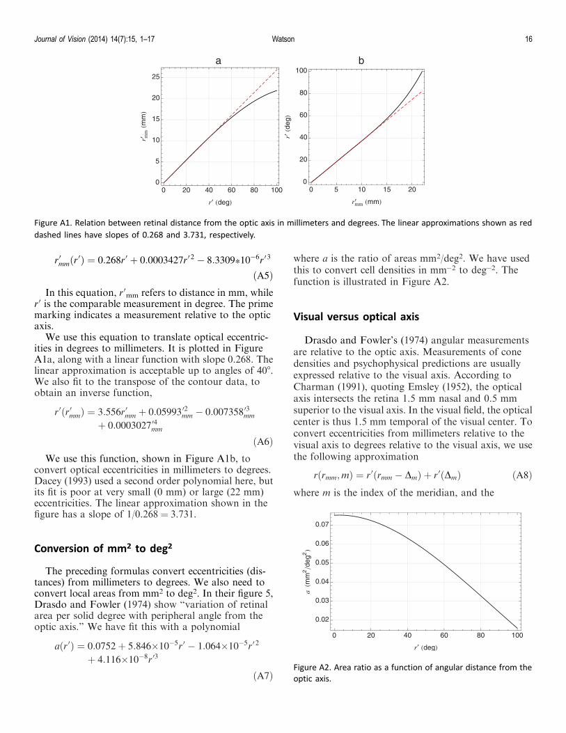
r0mm#r0$ " 0:268r0 % 0:0003427r02 ! 8:3309*10!6r03

#A5$In this equation, r0mm refers to distance in mm, while

r0 is the comparable measurement in degree. The primemarking indicates a measurement relative to the opticaxis.

We use this equation to translate optical eccentric-ities in degrees to millimeters. It is plotted in FigureA1a, along with a linear function with slope 0.268. Thelinear approximation is acceptable up to angles of 408.We also fit to the transpose of the contour data, toobtain an inverse function,

r0#r0mm$ " 3:556r0mm % 0:0599302mm ! 0:00735803

mm

% 0:000302704mm

#A6$We use this function, shown in Figure A1b, to

convert optical eccentricities in millimeters to degrees.Dacey (1993) used a second order polynomial here, butits fit is poor at very small (0 mm) or large (22 mm)eccentricities. The linear approximation shown in thefigure has a slope of 1/0.268" 3.731.

Conversion of mm2 to deg2

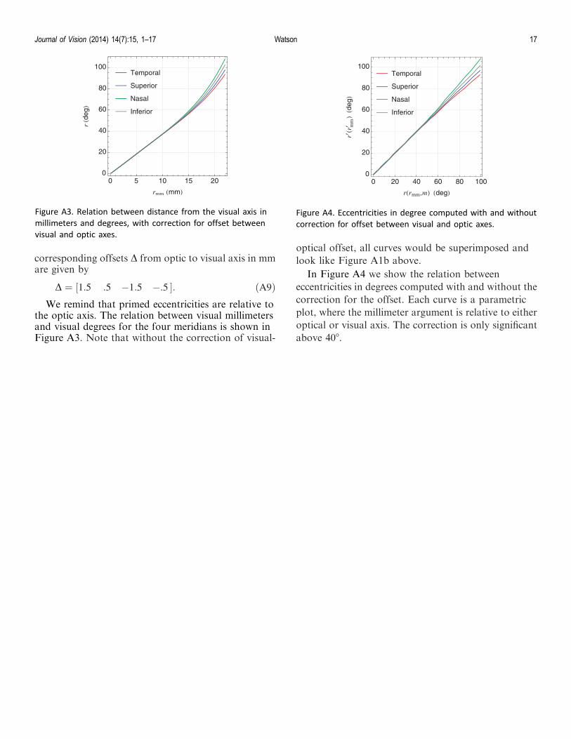
The preceding formulas convert eccentricities (dis-tances) from millimeters to degrees. We also need toconvert local areas from mm2 to deg2. In their figure 5,Drasdo and Fowler (1974) show ‘‘variation of retinalarea per solid degree with peripheral angle from theoptic axis.’’ We have fit this with a polynomial

a#r0$ " 0:0752% 5:846·10!5r0 ! 1:064·10!5r02

% 4:116·10!8r03

#A7$

where a is the ratio of areas mm2/deg2. We have usedthis to convert cell densities in mm!2 to deg!2. Thefunction is illustrated in Figure A2.

Visual versus optical axis

Drasdo and Fowler’s (1974) angular measurementsare relative to the optic axis. Measurements of conedensities and psychophysical predictions are usuallyexpressed relative to the visual axis. According toCharman (1991), quoting Emsley (1952), the opticalaxis intersects the retina 1.5 mm nasal and 0.5 mmsuperior to the visual axis. In the visual field, the opticalcenter is thus 1.5 mm temporal of the visual center. Toconvert eccentricities from millimeters relative to thevisual axis to degrees relative to the visual axis, we usethe following approximation

r#rmm;m$ " r0#rmm ! Dm$ % r0#Dm$ #A8$

where m is the index of the meridian, and the

Figure A1. Relation between retinal distance from the optic axis in millimeters and degrees. The linear approximations shown as red

dashed lines have slopes of 0.268 and 3.731, respectively.

Figure A2. Area ratio as a function of angular distance from the

optic axis.

Journal of Vision (2014) 14(7):15, 1–17 Watson 16

corresponding offsets D from optic to visual axis in mmare given by

D " 1:5 :5 !1:5 !:5& ': #A9$We remind that primed eccentricities are relative to

the optic axis. The relation between visual millimetersand visual degrees for the four meridians is shown inFigure A3. Note that without the correction of visual-

optical offset, all curves would be superimposed andlook like Figure A1b above.

In Figure A4 we show the relation betweeneccentricities in degrees computed with and without thecorrection for the offset. Each curve is a parametricplot, where the millimeter argument is relative to eitheroptical or visual axis. The correction is only significantabove 408.

Figure A3. Relation between distance from the visual axis in

millimeters and degrees, with correction for offset between

visual and optic axes.

Figure A4. Eccentricities in degree computed with and without

correction for offset between visual and optic axes.

Journal of Vision (2014) 14(7):15, 1–17 Watson 17