A forward modeling approach to paleoclimatic

interpretation of tree-ring data

M. N. Evans,1,2,3 B. K. Reichert,4,5 A. Kaplan,4 K. J. Anchukaitis,1,2 E. A. Vaganov,6

M. K. Hughes,1 and M. A. Cane4

Received 17 January 2006; accepted 24 May 2006; published 10 August 2006.

[1] We investigate the interpretation of tree-ring data using the Vaganov-Shashkinforward model of tree-ring formation. This model is derived from principles of coniferwood growth, and explicitly incorporates a nonlinear daily timescale model of themultivariate environmental controls on tree-ring growth. The model results are shown tobe robust with respect to primary moisture and temperature parameter choices. Whenapplied to the simulation of tree-ring widths from North America and Russia from theMann et al. (1998) and Vaganov et al. (2006) data sets, the forward model produces skillon annual and decadal timescales which is about the same as that achieved using classicaldendrochronological statistical modeling techniques. The forward model achieves thiswithout site-by-site tuning as is performed in statistical modeling. The results support theinterpretation of this broad-scale network of tree-ring width chronologies primarily asclimate proxies for use in statistical paleoclimatic field reconstructions, and point tofurther applications in climate science.

Citation: Evans, M. N., B. K. Reichert, A. Kaplan, K. J. Anchukaitis, E. A. Vaganov, M. K. Hughes, and M. A. Cane (2006),

A forward modeling approach to paleoclimatic interpretation of tree-ring data, J. Geophys. Res., 111, G03008, doi:10.1029/

2006JG000166.

1. Introduction

[2] A key element of climate change detection andattribution efforts is the determination of natural variabilityon timescales bracketing those of anthropogenic influenceson climate. In the absence of direct observations, especiallyprior to the rise of globally distributed direct observations inthe mid 19th century, we rely on the so-called ‘‘proxy’’climate indicators, which are often derived from geologicalor biological archives, and are interpreted by means ofstatistical relationships and chemical or biophysical princi-ples. One of the most widespread kinds of natural paleo-climatic archives are tree rings; data now exist from over2000 sites on six continents [World Data Center forPaleoclimatology, 2003]. The collection and interpretationof these data sets is based in biological principles of treegrowth [e.g., Schweingruber, 1988; Cook and Kairiukstis,1990; Fritts, 1991]. Subsequent analysis of derived paleo-

climate observational networks incorporating tree-ringrecords and other proxy data has produced hemisphericand global-scale paleoclimatic reconstructions over the pastfew centuries to millennia [e.g., Mann et al., 1998, 1999;Stahle et al., 1998; Briffa et al., 2001; Jones et al., 2001;Esper et al., 2002; Cook et al., 2002; Mann and Jones,2003].[3] Two major uncertainties lie in the statistical develop-

ment, analysis and interpretation of tree-ring data forpaleoclimate studies. First, there are nonclimatic influenceson tree-ring records, including tree biology, size, age andthe effects of localized forest dynamics [Cook andKairiukstis, 1990]. Successful elimination of these influen-ces is now routinely achieved via careful site selection,sampling, data analysis and a posteriori tests to ensure thatthe tree-ring record is dominated by the single climatevariable of interest. Perhaps of more concern is that tree-ring data reflect a nonlinear response to multivariate climateforcings. This represents a problem for both single-variablepaleoclimatic reconstructions via linear statistical calibra-tion of the tree-ring proxy data and for prediction of theeffects of climate change scenarios on tree biology andforest ecology. In both situations, statistical relationships,which may represent linearizations of nonlinear processes(see section 2), are difficult to validate for long periodprocesses and for times outside the instrumental era andmay not hold for paleoclimate or climate change experi-ments. For example, the application of statistical calibra-tions to an independent time period with a fundamentallydifferent climatic regime, for example, with comparabletemperatures but a general shift in water balance, may

JOURNAL OF GEOPHYSICAL RESEARCH, VOL. 111, G03008, doi:10.1029/2006JG000166, 2006ClickHere

for

FullArticle

1Laboratory of Tree-Ring Research, University of Arizona, Tucson,Arizona, USA.

2Also at Department of Geosciences, University of Arizona, Tucson,Arizona, USA.

3Also at Lamont-Doherty Earth Observatory, Columbia University,Palisades, New York, USA.

4Lamont-Doherty Earth Observatory, Columbia University, Palisades,New York, USA.

5Now at German Meteorological Service, Offenbach, Germany.6V. N. Sukachev Institute of Forest, Russian Academy of Sciences,

Krasnoyarsk, Russia.

Copyright 2006 by the American Geophysical Union.0148-0227/06/2006JG000166$09.00

G03008 1 of 13

consequently lead to an erroneous climate reconstruction[LaMarche et al., 1984; Graybill and Idso, 1993; Briffa etal., 1998; Vaganov et al., 1999; Barber et al., 2000;Kirdyanov et al., 2003; Anchukaitis et al., 2006]. Hencethe nature of trees as a biological archive of environmentalconditions raises questions about the validity of linear,statistical approaches to interpretation of the data.[4] Introduction of a process model of tree-ring growth,

from which tree ring formation is represented via firstprinciples of tree biology and climate data, permits us toinvestigate these issues directly. Here we investigate thepotential of the Vaganov-Shashkin model of tree-ring for-mation [Shashkin and Vaganov, 1993; Vaganov et al., 1990,2006] (see also E. A. Vaganov et al., Howwell understood arethe processes that create dendroclimatic records? A mech-anistic model of climatic control on conifer tree-ring growthdynamics, submitted to Dendroclimatology: Progress andProspects, edited byM. K. Hughes, T.W. Swetnam, and H. F.Diaz, Springer, 2006) (hereinafter referred to as Vaganov etal., submitted manuscript, 2006) to accurately simulate treesgrowing in a variety of environmental conditions. Althoughthere are several other process models of tree growth and ringformation [e.g., Fritts et al., 1999; Foster and LeBlanc, 1993;Misson, 2004], our interest in a robust if low-order forwardmodel with a prognostic variable directly comparable to stan-dard proxy observations led us to work with the Vaganov-Shashkin model. The tree-ring process model is brieflyreviewed in section 2. A more comprehensive descriptionof the development, theory, and justification of model com-ponents has recently been published by Vaganov et al. [2006,submitted manuscript, 2006]; the reader is referred to thismonograph for more details. This study, however, is a reportof the first broad-scale application of this model to thesimulation of tree-ring width data used for statistical paleo-climatology. The model is applied to the simulation of theactual tree-ring chronology data described in section 3.Performance of the model is reported in section 4. Theimplications of the results are discussed in section 5; con-clusions are summarized in section 6.

2. Model Description

2.1. General Principles

[5] The Vaganov-Shashkin model has two distinguishingfeatures. First, it deals with rates of growth of cells as if theirformation in the cambium is influenced exclusively by thephysical environment. This is a major simplification ofpresent knowledge of wood biology, made for the purposeof simplifying the model and reducing the number ofparameters. Second, it deals explicitly with the dynamicsof cell growth, division, and maturation in a dedicated‘‘cambial block’’ that is described briefly here and in detailelsewhere [Vaganov et al., 2006, submitted manuscript,2006]. This cambial block is driven by and is connectedwith the growth block. Thus the model simulates not onlythe width of conifer tree rings but also aspects of theirinternal structure, reflecting intraseasonal environmentalfluctuations.[6] The growth block of the Vaganov-Shashkin tree-ring

model uses the principle of limiting factors [e.g., Fritts,1991] to calculate conifer tree-ring formation integratedover the growing season from daily temperature, precipita-

tion, and sunlight. The daily growth rate on a specific day tis modeled as

G tð Þ ¼ gE tð Þmin gT tð Þ; gW tð Þ½ �;

where gE(t), gT(t), and gW(t) are the daily growth rates dueto solar radiation, near-surface air temperature, and soilwater balance, respectively. Dependence of growth on solarradiation gE(t) is a function of latitude, declination angle andhour angle [Gates, 1980, equation (6.10)]; any reduction ofgE by canopy shading has been neglected. The effects of theeccentricity of the Earth’s orbit around the Sun and ofatmospheric transmissivity have been neglected. Theminimum function permits tree-ring formation to vary ineffective functional dependence among temperature, moist-ure and sunlight on daily through seasonal timescales.Below, we briefly describe the component functionscontributing to G(t), as well as the environmentally drivencambial model. Much more detail on the VS model is foundin the literature [Vaganov et al., 1990, 1994; Vaganov, 1996;Vaganov et al., 1999, 2000]; a comprehensive review of itsdevelopment and application is given by Vaganov et al.[2006, submitted manuscript, 2006]. A schematic overviewof the model, its inputs and prognostics is given in Figure 1.Model parameters not varying in time, their assumed valuesand units are given in Table 1. These values were deter-mined from the literature and from intensive case studies ata limited number of sites [Vaganov et al., 2006, chap. 7](see also section 4.2 of this paper).

2.2. Growth Response to Temperature

[7] Experimental data [Fritts, 1976; Kramer andKozlowski, 1979; Gates, 1980; Lyr et al., 1992] suggestthat the dependence of the growth rate function ontemperature gT may be subdivided into three segments:(1) rising growth rates with increasing temperatures belowa growth-optimal temperature range; (2) relatively con-stant rates within an optimal range of temperatures; and(3) decreasing growth rates above that temperature range.This also represents the typical behavior of other biolog-ical systems. A polynomial function has been suggested[Vaganov et al., 1990; Fritts, 1991] which is approxi-mated in the Vaganov-Shashkin model by a piecewise linearfunction (Figure 1). Between the minimum temperaturefor growth Tmin and the lower end of the range of optimaltemperatures Topt1, the growth rate linearly increases withtemperature. Between Topt1 and Topt2, growth rate is optimalat a constant level, then decreasing linearly between Topt2 andthe maximum temperature for growth Tmax. Beyond Tmax,growth does not occur. Following studies by Lindsay andNewman [1956], Landsberg [1974], Valentine [1983],Cannell and Smith [1986], and Hanninen [1991], growth inthe model’s representation of cambial processes (see sec-tion 2.4) is initiated each year when the sum of dailytemperatures over a specified time period tbeg reaches a de-fined critical level Tbeg (Table 1).

2.3. Growth Response to Water Balance

[8] Similar to calculation of growth response to temper-ature gT(t), growth response to soil water balance gW(t) isalso expressed as a piecewise-linear function of W(Figure 1), which represents another approximation based

G03008 EVANS ET AL.: FORWARD MODELING OF TREE-RING RECORDS

2 of 13

G03008

on experimental data [Kramer and Kozlowski, 1979]. Thesoil water content W itself is calculated through a balanceequation for soil water dynamics [Thornthwaite and Mather,1955; Alisov, 1956],

dW ¼ f Pð Þ � E � Q:

Here dW is the daily change in soil water content, f(P) is afunction of daily precipitation, E is daily transpiration, andQ denotes daily runoff. Function f(P) is expressed as

f Pð Þ ¼ min c1P;Pmax½ �;

where P is the actual daily precipitation, the constant c1 isthe fraction of precipitation that is caught by the crown ofthe tree, and Pmax denotes the maximum level for saturatedsoil. In the case of temperatures near freezing, P is modifiedto allow for snow melt (if temperatures are above freezingand snow is present from prior-day calculations) or snowaccumulation (if temperatures are below freezing andprecipitation has occurred that day). For saturated soil,runoff Q is proportional to the soil water content W,

Q ¼ LW :

Figure 1. Schematic representation of the Vaganov-Shashkin tree-ring model (see section 2). Dailymodel inputs (solar radiation, temperature, and precipitation) are italicized.

Table 1. Tree-Ring Model Parameters Used Throughout This Study

Parameter Description (Units) Value

Tmin minimum temperature for tree growth (�C) 5.0Topt1 lower end of range of optimal temperatures (�C) 18.0Topt2 upper end of range of optimal temperatures (�C) 24.0Tmax maximum temperature for tree growth (�C) 31.0Wmin minimum soil moisture for tree growth, relative to saturated soil (v/vs) 0.04Wopt1 lower end of range of optimal soil moistures (v/vs) 0.2Wopt2 upper end of range of optimal soil moistures (v/vs) 0.8Wmax maximum soil moisture for tree growth (v/vs) 0.9Tbeg temperature sum for initiation of growth (� C) 60tbeg time period for temperature sum (days) 10lr depth of root system (mm) 1000Pmax maximum daily precip. for saturated soil (mm/day) 20c1 fraction of precipitation penetrating soil (not caught by crown) (rel. unit) 0.72c2 first coefficient for calculation of transpiration (mm/day) 0.12c3 second coefficient for calculation of transpiration (1/�C) 0.175L coefficient for water drainage from soil (dimensionless) 0.001tc cambial model time step (days) 0.2Vcr minimum cambial cell growth rate (mm/day) 0.04Do initial cambial cell size (mm) 4Dcr cell size at which mitotic cycle begins (mm) 8Vm growth rate during mitotic cycle (mm/day) 1Dm cambial cell size at which mitosis occurs (mm) 10

G03008 EVANS ET AL.: FORWARD MODELING OF TREE-RING RECORDS

3 of 13

G03008

The transpiration of water by the tree crown E dependsexponentially on temperature [Monteith and Unsworth,1990] and linearly on the growth function G,

E ¼ c2G tð Þ exp c3T½ �;

where the constants c2 and c3 are used to describe a variety oftree species and growth conditions (Table 1). The factorc2G(t) is related to stomatal conductance. In practice, thedependence of E on T is strongly constrained by the func-tional forms ofG, gTand gW (Figure 1 and Table 1; results notshown). For example, while a temperature increase into therange Topt1� Topt2 will increase gT, a concurrent temperature-driven increase in evapotranspiration will reduce soil mois-ture. The latter effect decreases W, and if W falls outside therange Wopt1 � Wopt2, leads to limitation of E by gW, via G.

2.4. Cambial Model

[9] In the component of the model which simulates thegrowth and formation of wood cells in the tree cambium,the daily growth rate is used to calculate the cellular growthrate Vi(t),

Vi tð Þ ¼ V0;iG tð Þ;

where the index i indicates the position in the cambial zoneof the growing cell, and V0,i is the linear dependence ofgrowth rate on position. Each cell is permitted to be dor-mant, grow, divide and/or differentiate into xylem on anintraday time interval tc. If the cell is not large enough todivide, and if Vi(t) is below a constant critical level Vcr, thecell is considered dormant and does not grow, divide ordifferentiate. If the cellular growth rate is greater than Vcr

but is less than a position-dependent minimum growth rateVmin [Fritts et al., 1999], then the cell can no longer divide,and exits the cambial zone. Otherwise, the cell grows froman initial size Do according to the environmentally scaledgrowth rate Vi(t) for that intraday interval. If the cell reachesor exceeds a critical cambial cell size Dcr, the cell must enterand complete the mitotic cycle. The cell now grows at anenvironmentally independent and constant growth rate Vm

until it reaches division size Dm. At this point, it is dividedinto two adjacent cells, each equal in size to one half of theparent cell size. At the end of the growing season (G ! 0),growth rate of the remaining cells in the cambial zone fallbelow Vcr and become dormant. They now represent theinitial cambial cells for the subsequent growing season.[10] In nature, tree-ring width (TRW) is determined by the

sum of the radial cell sizes of all cells produced during thegrowing season. In the version of the model that we used forthis study, however, TRW is estimated via the normalizednumber of noncambial cells N formed that year through theaforementioned processes of growth, division and differen-tiation (Figure 1, top two lines). This is possible becausethere is always a strong linear relationship between N andTRW [Gregory, 1971; Vaganov et al., 1985; Camerero et al.,1998; Wang et al., 2002; Vaganov et al., 2006, submittedmanuscript, 2006]. Hence, in the model simulation,

TRW tð Þ ¼ N

hNit;

where t is now time interval in units of annual growingseasons, and h. . .it indicates the time average over the entiresimulation. The simulated standardized (dimensionless)tree-ring width chronologies may then be directly comparedto actual standardized tree-ring width data.

2.5. Model Operationalization

[11] The Vaganov-Shashkin model is integrated in thefollowing manner.[12] 1. The overall growth function G is calculated on the

basis of current gE, gT and gW. Here gE depends on latitudeand time; gT depends on current-day T; gW depends on aninitial or prior-day W and dW, which in turn are based onprecipitation, soil drainage, and snowmelt or accumulation.[13] 2. The cambial growth rate Vi(G) is calculated for

each cambial cell left at the end of the prior growing season,or for each cambial cell from the prior day’s calculation. Inall simulations described here, the cambial model time stepwas 1/5 day. Depending on the value of Vi(G) relative to Vcr

and Vmin, each cell goes dormant, grows, differentiates intoxylem, or divides at each cambial time step.[14] 3. On the basis of the precipitation function f(P),

calculated E, T, and the growth function G, the change insoil moisture dW = f(P) � E � Q is calculated. W(t + 1) =W(t) + dW(t) is calculated for use in the following day’ssimulation.[15] 4. The model continues for the following day of the

year. At the end of the year t, TRW is calculated from thenumber of noncambial cells produced over the course ofthe growing season. The number and size of each cambialcell is used as input for the following year’s simulation. Atthe end of the simulation time interval, TRW is normalizedby the mean TRW for all years of the simulation.

3. Data and Methods

3.1. Tree-Ring Chronologies

[16] At present, there are over 2000 tree-ring chronolo-gies potentially available for intercomparison with syntheticchronologies produced by the tree-ring model [World DataCenter for Paleoclimatology, 2003; Contributors of theInternational Tree Ring Data Bank, 2002]. However, someof these chronologies were developed for purposes otherthan paleoclimatic reconstruction, others lack sufficientreplication, and yet others were standardized in ways whichmight limit paleoclimatic interpretation of the data. Hencewe selected 198 tree-ring width chronologies for compari-son with the tree-ring model output from two sources. Allrepresent site averages of multiple raw ring width series(‘‘chronologies’’) dated to the calendar year and statisticallyfiltered by the data developers [Contributors of the Inter-national Tree Ring Data Bank, 2002] to remove purely agedependent time series features. Of these, 190 data series forNorth America are from the Mann et al. [1998] data set.These data were screened a priori for several quality controlvariables [Mann et al., 2000] to produce a data set mostconducive to paleoclimate reconstruction, and represent anexcellent target for this study. Data from eight sites inRussia are from published or unpublished data sets devel-oped by Vaganov et al. [1999, 2006, submitted manuscript,2006].

G03008 EVANS ET AL.: FORWARD MODELING OF TREE-RING RECORDS

4 of 13

G03008

3.2. Tree-Ring Width Simulations

[17] Daily station records from the comprehensive GlobalHistorical Climatology Network [Peterson and Vose, 1997]data set are used to simulate tree-ring chronologies at NorthAmerican locations. Daily weather station data for Russianchronology locations is obtained by the Institute of Forest ofthe Russian Academy of Sciences, Krasnoyarsk, Russia(V. Shishov, personal communication, 2005). Missing tem-perature data are replaced by linearly interpolated values.Missing precipitation data were simply set to zero. In thecase of more than 90 days of missing meteorological data,the year was not simulated. To account for model equili-bration, all model simulations were initialized with the samedefault number of cambial cells and sizes, and initial soilmoisture values, and the first modeled year’s growth wasdiscarded. The simulated growth following a missing me-teorological year was initialized using the last simulatedyear’s initialization file, and the first year following ameteorological hiatus was discarded as well.[18] We note that meteorological station proximity may

not always be the best criterion for selecting the appropriatetree-ring model input. For example, the presence of orog-raphy produces spatially isentropic features into patterns oftemperature and rainfall on daily to seasonal timescales, andelevation differences between tree-ring sites and meteoro-logical stations may artificially create large differencesbetween actual and simulated chronologies. For these rea-sons, we attempt to partially correct temperature for eleva-tional differences by using an adiabatic correction(6.6�C/km; [Wallace and Hobbs, 1977]) for the meanelevation difference between our set of actual tree-ringchronologies and the meteorological stations. On average,chronologies are located 700 m higher than stations; thusthe mean temperature correction of 4.6�C was used for all

North American simulations. We then simulated the 190North American tree-ring width chronologies for all mete-orological stations found within a 500-km search radius,and the eight Russian chronologies using meteorologicaldata from the nearest station [Vaganov et al., 2006, submit-ted manuscript, 2006]. In reporting results for each of the190 North American sites, we use the simulation for thestation found within the 500-km search radius that is mostsignificantly correlated with the given actual tree ring widthdata series over the full intercomparison period available.This period averaged 1915–1981. For the eight Russiansites the meteorological station data coverage is sparser, andwe report the same statistic but for correlation with theclosest meteorological station, and without a mean temper-ature correction.[19] It is also important to note the rather simplistic

approach taken with this application of the process model.The model itself is only a very simple depiction of treegrowth [Vaganov et al., 2006, submitted manuscript, 2006].For example, the model does not explicitly include photo-synthesis, and it does not include other possibly importantcontrols on tree growth, such as atmospheric attenuationof solar radiation, nutrient availability, CO2 fertilization,long-term dependence of tree-ring width on tree age, oranthropogenic influences on growth conditions, except asmirrored in meteorological station temperature and precip-itation. In addition we did not tune the model fixed pa-rameters by region, mean climate, or species; all model runsuse the parameter values listed in Table 1. However,precisely owing to the simplicity of the model and experi-mental conditions, we can test, in the sense of Occam’srazor, the hypothesis that observed tree-ring variations aredue solely to meteorological controls, as represented in theVaganov-Shashkin model. The same assumption implicitly

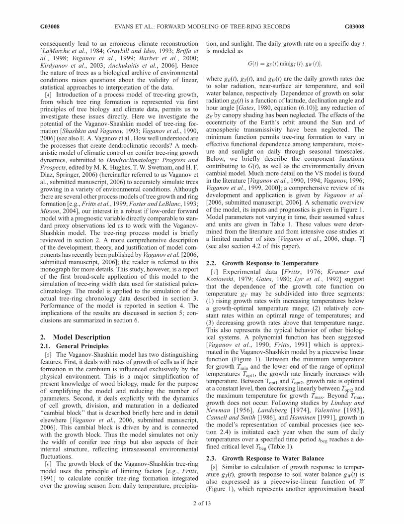
Figure 2. Seasonal soil moisture and temperature controls on simulated tree-ring growth at Ulan-Ude,southern Siberia, 1982–1986. (a, b) Daily temperature T (�C) and precipitation P (mm/day) used to drivethe model. (c) Soil moisture W calculated by the water balance component of the model (volume/volumeratio). (d) Annual dimensionless growth response function G(t). (e) Cumulative number of tracheids(wood cells) N per ring for each year’s growing season.

G03008 EVANS ET AL.: FORWARD MODELING OF TREE-RING RECORDS

5 of 13

G03008

underlies many uses of tree-ring data in paleoclimatereconstructions.

4. Results

4.1. Model Behavior: Ulan-Ude, Southern Russia

[20] Figure 2 illustrates a single time series ring widthsimulation (Ulan-Ude, Buryatia region, southern Siberia:51.8�N, 107.6�E; 510 m elevation) in terms of the intra-annual contributions of the temperature and moisturegrowth functions for a recent 5-year interval. The model’ssimulation of annual ring widths is compared to data from aScots pine (Pinus sylvestris L.) tree-ring width chronology[Andreev et al., 1999] from the same region for the period1922–1989 (Figure 3).[21] Tree growth for this site is expected to be mainly

sensitive to the availability of water, although for specifictime periods temperature can become an important factor. In1985, the beginning of the growth season (which the modeldefines as when the temperature sum over the period tbeg =10 days has reached the critical level of 60�C (Table 1) is inMay (Figure 2). The growth function remains high until theend of June, due to net positive precipitation-evaporation inMay and June. A relatively dry period is observed fromearly July until the end of August. The consequence is a netdecrease in available water during that period, resulting in adrastic decrease of the growth function. Although greaterprecipitation is received in the fall, the growth function issubsequently limited by temperature as the growing seasondraws to a close. The resulting ring width over the year can,as a first approximation, be seen as the integration over thegrowth function and shows a relatively wide ring for thisyear, mainly due to favorable growing conditions until theend of June. By contrast, 1987 shows much lower precip-itation within the growth season window defined by theannual cycle of temperature. Consequently, soil moisturewas lower throughout the growing season, and the

integrated growth function indicates a much narrowerpredicted tree ring.[22] The observed and simulated annual tree-ring indices

for the available intercomparison period 1922–1986, to-gether with their 5-year running means, are shown inFigure 3. The correlation coefficients for annual data and5-year averages are r = 0.58 and r = 0.65, respectively; bothcorrelations are significant at the 99% level. The simulatedindex for the first year, 1922, does not agree with theobservation due to the arbitrariness of model initialization.For other years, the agreement is generally good, with theexception of the years 1933, 1941, 1944, and 1969. Themisfit to the tree-ring chronology, especially in 1969,generally coincides with periods when large amounts ofdaily weather data are missing.

4.2. Model Sensitivity: Ulan-Ude, Southern Russia

[23] To evaluate the sensitivity of the Ulan-Ude results tomodel parameters which define the temperature and waterbalance growth functions (Figure 1), we performed twoadditional experiments (Figure 4). For the first experiment,we varied one of the parameters Tmin, Topt1, Topt2, and Tmax,keeping all other parameters constant. The value of each ofthe varied four parameters (Table 1) was increased anddecreased stepwise (steps of ±0.5�C) up to a change of±5�C, and the simulations were repeated for each newparameter set, resulting in a total of 80 simulated chronol-ogies, which could then be compared to the actual tree-ringchronology from Ulan-Ude. Similarly, the values for Wmin,Wopt1, Wopt2, and Wmax were varied over a range of ±20%and the simulated chronologies compared to the actualchronology.[24] We found that the tree-ring width simulation for

Ulan-Ude was not very sensitive to the choice of primarytemperature and water budget parameters (Figures 2 and 4).Decreasing the parameters Tmin and Topt1 have virtually noeffect on the simulation; an increase in any of theseparameters results in slightly lower but not significantlydifferent correlation coefficients (Figure 4a). Only a de-crease of Topt2 and Tmax result in significantly lowercorrelations, suggesting that lower values for the upperbranch of the temperature growth function are unrealistic,consistent with experimental data [e.g., Gates, 1980; Lyr etal., 1992]. The second experiment examined the response tovariation of the water balance parametersWmin,Wopt1,Wopt2,and Wmax in the same manner, to ±20% of their originalvalues (Table 1). As Wopt2 and Wmax are varied, correlationsremain at a constant level for all experiments (Figure 4b),indicating that the soil water balance does not approach alevel of saturation that would negatively affect tree ringgrowth at this site at any time. The important parametersaffecting model output here are Wmin and Wopt1. Increasingthe values for Wopt1 does not have a significant influence,whereas increasing Wmin (the lowest soil water level for theoccurrence of growth) seems to have an optimum aroundthe original value. A decrease of either parameter by 20%results in a drop of the correlation coefficient from roughly0.6 to about 0.3, demonstrating the sensitivity of the modelto the lower part of the water balance growth function(Figure 2b). This is consistent with the presumption thattree-ring growth of the investigated chronology is mainlylimited by the availability of water.

Figure 3. Observed and simulated tree-ring width indices,Ulan-Ude, 1922–1986. Annual (thin lines) and 5-year mean(thick lines) correlations are r = 0.58 and r = 0.65,respectively, both significant at the 99% level for theeffective numbers of degrees of freedom.

G03008 EVANS ET AL.: FORWARD MODELING OF TREE-RING RECORDS

6 of 13

G03008

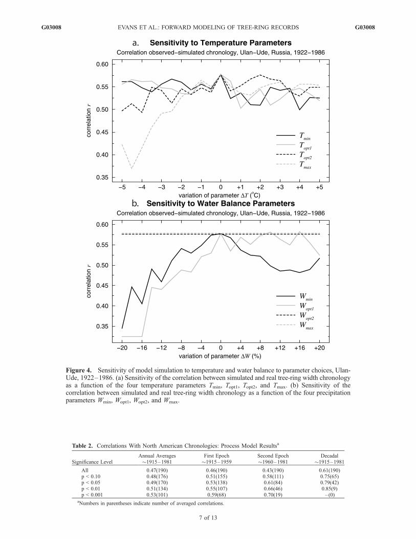
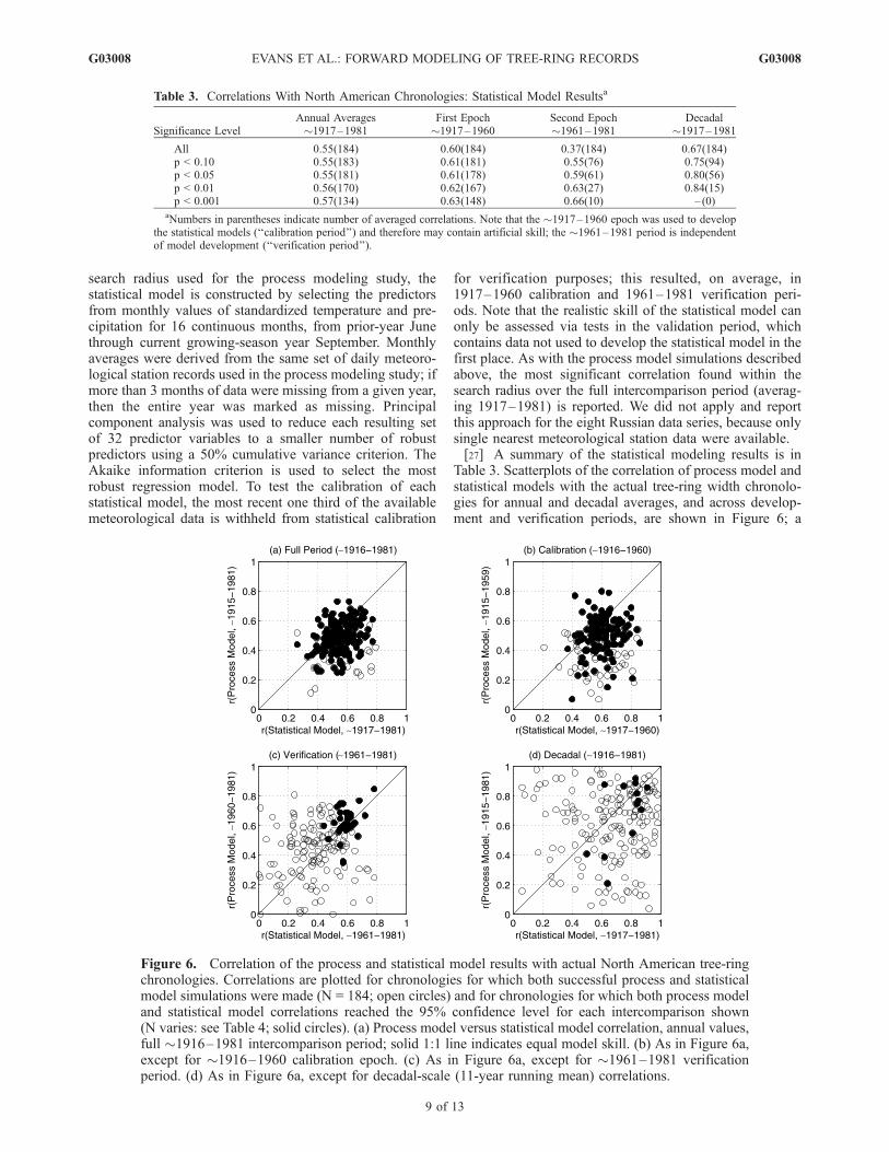
Table 2. Correlations With North American Chronologies: Process Model Resultsa

Significance LevelAnnual Averages1915–1981

First Epoch1915–1959

Second Epoch1960–1981

Decadal1915–1981

All 0.47(190) 0.46(190) 0.43(190) 0.61(190)p < 0.10 0.48(176) 0.51(155) 0.58(111) 0.75(65)p < 0.05 0.49(170) 0.53(138) 0.61(84) 0.79(42)p < 0.01 0.51(134) 0.55(107) 0.66(46) 0.85(9)p < 0.001 0.53(101) 0.59(68) 0.70(19) – (0)

aNumbers in parentheses indicate number of averaged correlations.

Figure 4. Sensitivity of model simulation to temperature and water balance to parameter choices, Ulan-Ude, 1922–1986. (a) Sensitivity of the correlation between simulated and real tree-ring width chronologyas a function of the four temperature parameters Tmin, Topt1, Topt2, and Tmax. (b) Sensitivity of thecorrelation between simulated and real tree-ring width chronology as a function of the four precipitationparameters Wmin, Wopt1, Wopt2, and Wmax.

G03008 EVANS ET AL.: FORWARD MODELING OF TREE-RING RECORDS

7 of 13

G03008

4.3. Simulation of Actual Ring Width Chronologies

[25] A third set of results demonstrates generalized modelbehavior, as represented by the quality of simulation of theentire set of 198 chronologies described in section 2. Wecalculate the significance of correlations between all simu-lated and actual chronologies on annual and decadal(11-year running mean) timescales (Table 2 and Figure 5),taking into account the reduction in effective degrees offreedom due to autocorrelation and temporal averaging[Trenberth, 1984; Donaldson and Tryon, 1987]; for eachchronology, we report the process model correlation havingthe highest significance within the 500-km search radiusover the full intercomparison period. Figure 5 shows themap of the significance of correlations between the 198simulated and real tree ring chronology data series. A goodfit is found across the entire data set, which includeschronologies from the arid western United States, Siberiaas well as from the humid, warm eastern United States, andseveral different species of trees. Table 2 shows the corre-lation of the 190 North American simulated chronologies onannual and decadal timescales, and for the two epochs

(1915–1959 and 1960–1981) of the average common1915–1981 intercomparison timeframe. The average corre-lation for all stations over the full period is 0.47. 176 of 190annual-scale correlations between process-modeled andobserved tree-ring width chronologies are significant atthe 95% confidence level, with an average correlation of0.49. Furthermore, the annual correlations are stable withrespect to the two chosen epochs (Table 2): The correlationaverages are 0.46 and 0.43 in each of these periods. Ondecadal timescales, the average correlation is 0.61 for allmodeled chronologies, the average of the 42 of 190 corre-lations significant at the 95% confidence level is 0.79.

4.4. Skill Intercomparison: Process and StatisticalModeling

[26] A fourth set of results allows us to assess the processmodel skill relative to that of multivariate linear statisticalmodels developed using a standard dendroclimatologicalapproach [e.g., Guiot, 1990; Fritts, 1991; Cook et al.,1999]. For each of the prewhitened 190 North Americanchronology data series, for all sites within the same 500-km

Figure 5. Correlation significance map for simulation of 198 tree ring width chronologies from NorthAmerica and Russia for the 1915–1981 comparison period. Significance levels (considering effectivedegrees of freedom): >99% (black circles; n = 138; 70% of correlations), >95% (gray circles; n = 174;88% of correlations), <95% (white circles; n = 24; 12% of correlations).

G03008 EVANS ET AL.: FORWARD MODELING OF TREE-RING RECORDS

8 of 13

G03008

search radius used for the process modeling study, thestatistical model is constructed by selecting the predictorsfrom monthly values of standardized temperature and pre-cipitation for 16 continuous months, from prior-year Junethrough current growing-season year September. Monthlyaverages were derived from the same set of daily meteoro-logical station records used in the process modeling study; ifmore than 3 months of data were missing from a given year,then the entire year was marked as missing. Principalcomponent analysis was used to reduce each resulting setof 32 predictor variables to a smaller number of robustpredictors using a 50% cumulative variance criterion. TheAkaike information criterion is used to select the mostrobust regression model. To test the calibration of eachstatistical model, the most recent one third of the availablemeteorological data is withheld from statistical calibration

for verification purposes; this resulted, on average, in1917–1960 calibration and 1961–1981 verification peri-ods. Note that the realistic skill of the statistical model canonly be assessed via tests in the validation period, whichcontains data not used to develop the statistical model in thefirst place. As with the process model simulations describedabove, the most significant correlation found within thesearch radius over the full intercomparison period (averag-ing 1917–1981) is reported. We did not apply and reportthis approach for the eight Russian data series, because onlysingle nearest meteorological station data were available.[27] A summary of the statistical modeling results is in

Table 3. Scatterplots of the correlation of process model andstatistical models with the actual tree-ring width chronolo-gies for annual and decadal averages, and across develop-ment and verification periods, are shown in Figure 6; a

Table 3. Correlations With North American Chronologies: Statistical Model Resultsa

Significance LevelAnnual Averages1917–1981

First Epoch1917–1960

Second Epoch1961–1981

Decadal1917–1981

All 0.55(184) 0.60(184) 0.37(184) 0.67(184)p < 0.10 0.55(183) 0.61(181) 0.55(76) 0.75(94)p < 0.05 0.55(181) 0.61(178) 0.59(61) 0.80(56)p < 0.01 0.56(170) 0.62(167) 0.63(27) 0.84(15)p < 0.001 0.57(134) 0.63(148) 0.66(10) – (0)

aNumbers in parentheses indicate number of averaged correlations. Note that the 1917–1960 epoch was used to developthe statistical models (‘‘calibration period’’) and therefore may contain artificial skill; the 1961–1981 period is independentof model development (‘‘verification period’’).

Figure 6. Correlation of the process and statistical model results with actual North American tree-ringchronologies. Correlations are plotted for chronologies for which both successful process and statisticalmodel simulations were made (N = 184; open circles) and for chronologies for which both process modeland statistical model correlations reached the 95% confidence level for each intercomparison shown(N varies: see Table 4; solid circles). (a) Process model versus statistical model correlation, annual values,full 1916–1981 intercomparison period; solid 1:1 line indicates equal model skill. (b) As in Figure 6a,except for 1916–1960 calibration epoch. (c) As in Figure 6a, except for 1961–1981 verificationperiod. (d) As in Figure 6a, except for decadal-scale (11-year running mean) correlations.

G03008 EVANS ET AL.: FORWARD MODELING OF TREE-RING RECORDS

9 of 13

G03008

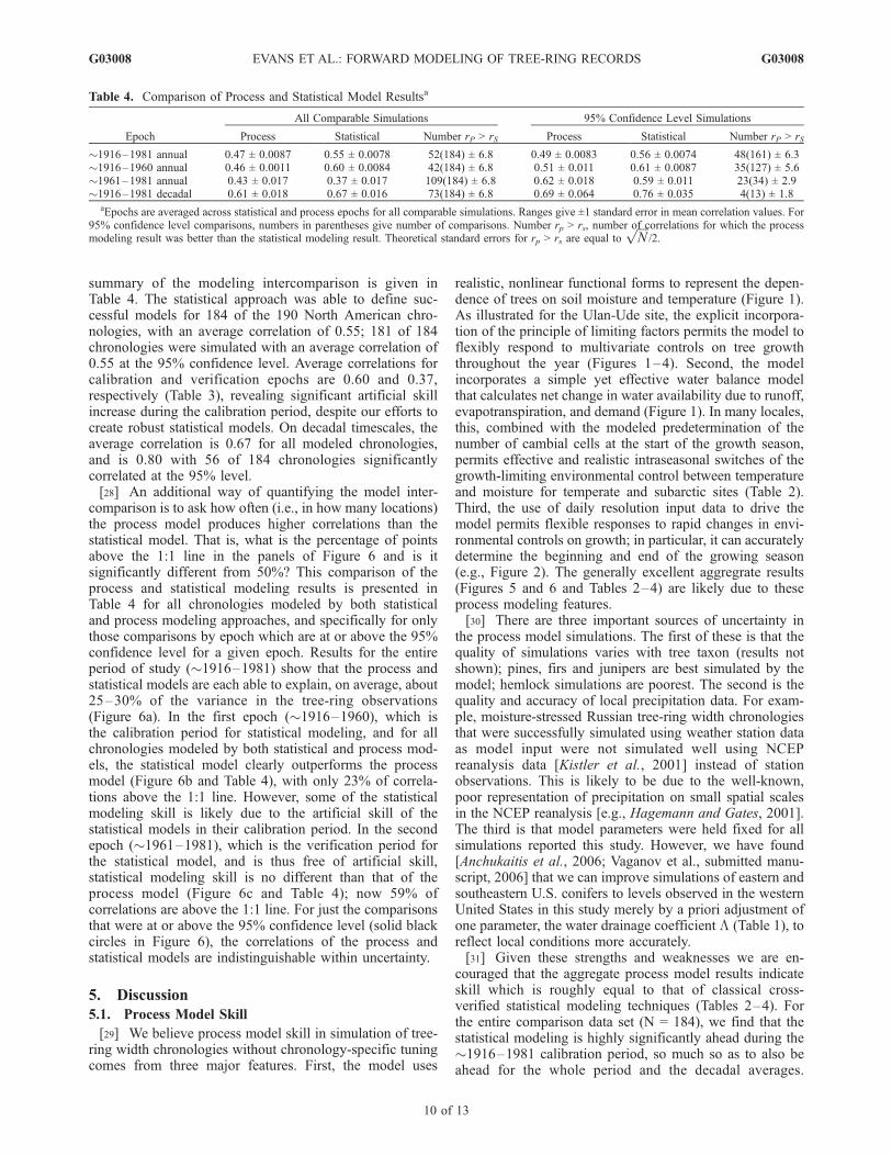
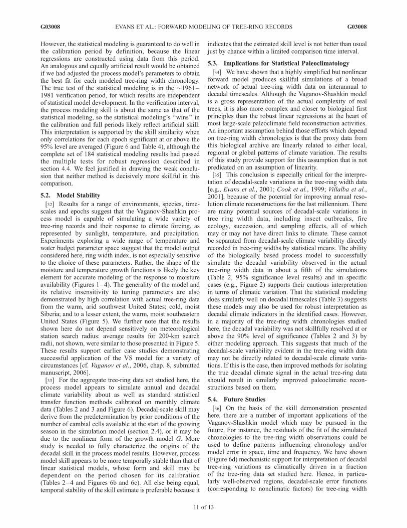
summary of the modeling intercomparison is given inTable 4. The statistical approach was able to define suc-cessful models for 184 of the 190 North American chro-nologies, with an average correlation of 0.55; 181 of 184chronologies were simulated with an average correlation of0.55 at the 95% confidence level. Average correlations forcalibration and verification epochs are 0.60 and 0.37,respectively (Table 3), revealing significant artificial skillincrease during the calibration period, despite our efforts tocreate robust statistical models. On decadal timescales, theaverage correlation is 0.67 for all modeled chronologies,and is 0.80 with 56 of 184 chronologies significantlycorrelated at the 95% level.[28] An additional way of quantifying the model inter-

comparison is to ask how often (i.e., in how many locations)the process model produces higher correlations than thestatistical model. That is, what is the percentage of pointsabove the 1:1 line in the panels of Figure 6 and is itsignificantly different from 50%? This comparison of theprocess and statistical modeling results is presented inTable 4 for all chronologies modeled by both statisticaland process modeling approaches, and specifically for onlythose comparisons by epoch which are at or above the 95%confidence level for a given epoch. Results for the entireperiod of study (1916–1981) show that the process andstatistical models are each able to explain, on average, about25–30% of the variance in the tree-ring observations(Figure 6a). In the first epoch (1916–1960), which isthe calibration period for statistical modeling, and for allchronologies modeled by both statistical and process mod-els, the statistical model clearly outperforms the processmodel (Figure 6b and Table 4), with only 23% of correla-tions above the 1:1 line. However, some of the statisticalmodeling skill is likely due to the artificial skill of thestatistical models in their calibration period. In the secondepoch (1961–1981), which is the verification period forthe statistical model, and is thus free of artificial skill,statistical modeling skill is no different than that of theprocess model (Figure 6c and Table 4); now 59% ofcorrelations are above the 1:1 line. For just the comparisonsthat were at or above the 95% confidence level (solid blackcircles in Figure 6), the correlations of the process andstatistical models are indistinguishable within uncertainty.

5. Discussion

5.1. Process Model Skill

[29] We believe process model skill in simulation of tree-ring width chronologies without chronology-specific tuningcomes from three major features. First, the model uses

realistic, nonlinear functional forms to represent the depen-dence of trees on soil moisture and temperature (Figure 1).As illustrated for the Ulan-Ude site, the explicit incorpora-tion of the principle of limiting factors permits the model toflexibly respond to multivariate controls on tree growththroughout the year (Figures 1–4). Second, the modelincorporates a simple yet effective water balance modelthat calculates net change in water availability due to runoff,evapotranspiration, and demand (Figure 1). In many locales,this, combined with the modeled predetermination of thenumber of cambial cells at the start of the growth season,permits effective and realistic intraseasonal switches of thegrowth-limiting environmental control between temperatureand moisture for temperate and subarctic sites (Table 2).Third, the use of daily resolution input data to drive themodel permits flexible responses to rapid changes in envi-ronmental controls on growth; in particular, it can accuratelydetermine the beginning and end of the growing season(e.g., Figure 2). The generally excellent aggregrate results(Figures 5 and 6 and Tables 2–4) are likely due to theseprocess modeling features.[30] There are three important sources of uncertainty in

the process model simulations. The first of these is that thequality of simulations varies with tree taxon (results notshown); pines, firs and junipers are best simulated by themodel; hemlock simulations are poorest. The second is thequality and accuracy of local precipitation data. For exam-ple, moisture-stressed Russian tree-ring width chronologiesthat were successfully simulated using weather station dataas model input were not simulated well using NCEPreanalysis data [Kistler et al., 2001] instead of stationobservations. This is likely to be due to the well-known,poor representation of precipitation on small spatial scalesin the NCEP reanalysis [e.g., Hagemann and Gates, 2001].The third is that model parameters were held fixed for allsimulations reported this study. However, we have found[Anchukaitis et al., 2006; Vaganov et al., submitted manu-script, 2006] that we can improve simulations of eastern andsoutheastern U.S. conifers to levels observed in the westernUnited States in this study merely by a priori adjustment ofone parameter, the water drainage coefficient L (Table 1), toreflect local conditions more accurately.[31] Given these strengths and weaknesses we are en-

couraged that the aggregate process model results indicateskill which is roughly equal to that of classical cross-verified statistical modeling techniques (Tables 2–4). Forthe entire comparison data set (N = 184), we find that thestatistical modeling is highly significantly ahead during the1916–1981 calibration period, so much so as to also beahead for the whole period and the decadal averages.

Table 4. Comparison of Process and Statistical Model Resultsa

Epoch

All Comparable Simulations 95% Confidence Level Simulations

Process Statistical Number rP > rS Process Statistical Number rP > rS

1916–1981 annual 0.47 ± 0.0087 0.55 ± 0.0078 52(184) ± 6.8 0.49 ± 0.0083 0.56 ± 0.0074 48(161) ± 6.31916–1960 annual 0.46 ± 0.0011 0.60 ± 0.0084 42(184) ± 6.8 0.51 ± 0.011 0.61 ± 0.0087 35(127) ± 5.61961–1981 annual 0.43 ± 0.017 0.37 ± 0.017 109(184) ± 6.8 0.62 ± 0.018 0.59 ± 0.011 23(34) ± 2.91916–1981 decadal 0.61 ± 0.018 0.67 ± 0.016 73(184) ± 6.8 0.69 ± 0.064 0.76 ± 0.035 4(13) ± 1.8

aEpochs are averaged across statistical and process epochs for all comparable simulations. Ranges give ±1 standard error in mean correlation values. For95% confidence level comparisons, numbers in parentheses give number of comparisons. Number rp > rs, number of correlations for which the processmodeling result was better than the statistical modeling result. Theoretical standard errors for rp > rs are equal to

ffiffiffiffi

Np

/2.

G03008 EVANS ET AL.: FORWARD MODELING OF TREE-RING RECORDS

10 of 13

G03008

However, the statistical modeling is guaranteed to do well inthe calibration period by definition, because the linearregressions are constructed using data from this period.An analogous and equally artificial result would be obtainedif we had adjusted the process model’s parameters to obtainthe best fit for each modeled tree-ring width chronology.The true test of the statistical modeling is in the 1961–1981 verification period, for which results are independentof statistical model development. In the verification interval,the process modeling skill is about the same as that of thestatistical modeling, so the statistical modeling’s ‘‘wins’’ inthe calibration and full periods likely reflect artificial skill.This interpretation is supported by the skill similarity whenonly correlations for each epoch significant at or above the95% level are averaged (Figure 6 and Table 4), although thecomplete set of 184 statistical modeling results had passedthe multiple tests for robust regression described insection 4.4. We feel justified in drawing the weak conclu-sion that neither method is decisively more skillful in thiscomparison.

5.2. Model Stability

[32] Results for a range of environments, species, time-scales and epochs suggest that the Vaganov-Shashkin pro-cess model is capable of simulating a wide variety oftree-ring records and their response to climate forcing, asrepresented by sunlight, temperature, and precipitation.Experiments exploring a wide range of temperature andwater budget parameter space suggest that the model outputconsidered here, ring width index, is not especially sensitiveto the choice of these parameters. Rather, the shape of themoisture and temperature growth functions is likely the keyelement for accurate modeling of the response to moistureavailability (Figures 1–4). The generality of the model andits relative insensitivity to tuning parameters are alsodemonstrated by high correlation with actual tree-ring datafrom the warm, arid southwest United States; cold, moistSiberia; and to a lesser extent, the warm, moist southeasternUnited States (Figure 5). We further note that the resultsshown here do not depend sensitively on meteorologicalstation search radius: average results for 200-km searchradii, not shown, were similar to those presented in Figure 5.These results support earlier case studies demonstratingsuccessful application of the VS model for a variety ofcircumstances [cf. Vaganov et al., 2006, chap. 8, submittedmanuscript, 2006].[33] For the aggregate tree-ring data set studied here, the

process model appears to simulate annual and decadalclimate variability about as well as standard statisticaltransfer function methods calibrated on monthly climatedata (Tables 2 and 3 and Figure 6). Decadal-scale skill mayderive from the predetermination by prior conditions of thenumber of cambial cells available at the start of the growingseason in the simulation model (section 2.4), or it may bedue to the nonlinear form of the growth model G. Morestudy is needed to fully characterize the origins of thedecadal skill in the process model results. However, processmodel skill appears to be more temporally stable than that oflinear statistical models, whose form and skill may bedependent on the period chosen for its calibration(Tables 2–4 and Figures 6b and 6c). All else being equal,temporal stability of the skill estimate is preferable because it

indicates that the estimated skill level is not better than usualjust by chance within a limited comparison time interval.

5.3. Implications for Statistical Paleoclimatology

[34] We have shown that a highly simplified but nonlinearforward model produces skillful simulations of a broadnetwork of actual tree-ring width data on interannual todecadal timescales. Although the Vaganov-Shashkin modelis a gross representation of the actual complexity of realtrees, it is also more complex and closer to biological firstprinciples than the robust linear regressions at the heart ofmost large-scale paleoclimate field reconstruction activities.An important assumption behind those efforts which dependon tree-ring width chronologies is that the proxy data fromthis biological archive are linearly related to either local,regional or global patterns of climate variation. The resultsof this study provide support for this assumption that is notpredicated on an assumption of linearity.[35] This conclusion is especially critical for the interpre-

tation of decadal-scale variations in the tree-ring width data[e.g., Evans et al., 2001; Cook et al., 1999; Villalba et al.,2001], because of the potential for improving annual reso-lution climate reconstructions for the last millennium. Thereare many potential sources of decadal-scale variations intree ring width data, including insect outbreaks, fireecology, succession, and sampling effects, all of whichmay or may not have direct links to climate. These cannotbe separated from decadal-scale climate variability directlyrecorded in tree-ring widths by statistical means. The abilityof the biologically based process model to successfullysimulate the decadal variability observed in the actualtree-ring width data in about a fifth of the simulations(Table 2, 95% significance level results) and in specificcases (e.g., Figure 2) supports their cautious interpretationin terms of climatic variation. That the statistical modelingdoes similarly well on decadal timescales (Table 3) suggeststhese models may also be used for robust interpretation asdecadal climate indicators in the identified cases. However,in a majority of the tree-ring width chronologies studiedhere, the decadal variability was not skillfully resolved at orabove the 90% level of significance (Tables 2 and 3) byeither modeling approach. This suggests that much of thedecadal-scale variability evident in the tree-ring width datamay not be directly related to decadal-scale climate varia-tions. If this is the case, then improved methods for isolatingthe true decadal climate signal in the actual tree-ring datashould result in similarly improved paleoclimatic recon-structions based on them.

5.4. Future Studies

[36] On the basis of the skill demonstration presentedhere, there are a number of important applications of theVaganov-Shashkin model which may be pursued in thefuture. For instance, the residuals of the fit of the simulatedchronologies to the tree-ring width observations could beused to define patterns influencing chronology and/ormodel error in space, time and frequency. We have shown(Figure 6d) mechanistic support for interpretation of decadaltree-ring variations as climatically driven in a fractionof the tree-ring data set studied here. Hence, in particu-larly well-observed regions, decadal-scale error functions(corresponding to nonclimatic factors) for tree-ring width

G03008 EVANS ET AL.: FORWARD MODELING OF TREE-RING RECORDS

11 of 13

G03008

records might be identified. This would represent a signif-icant step toward validating and improving statisticallybased but ultimately subjective data standardization techni-ques and identifying decadal climate variability reliably.With the error functions of model and data better resolved,especially on interannual to decadal timescales, we caninvestigate the inversion of data and model for simultaneoustemperature and precipitation reconstructions. GCM outputcould be used to hindcast probabilistically the naturalvariability in growth of conifer forest ecosystems andcarbon budgets on a global scale. Similarly, climate changeforecasts may be transformed into a global conifer forestchange ‘‘fingerprint’’ [Vaganov et al., 2006, submittedmanuscript, 2006], and the results compared to ongoingsatellite observations of the terrestrial ecosystem. These lat-ter applications would require a simulation model expandedto include the effects of changing atmospheric concentra-tions of carbon dioxide on tree growth.

6. Conclusions

[37] We have found the Vaganov-Shashkin modelcapable of accurately simulating intraseasonal to interde-cadal climate variability, as expressed in variations intree-ring width, for large regions of North American andRussia. The process model is relatively insensitive toparameter estimation, as shown by the good simulationof actual tree-ring width chronologies from a variety ofenvironments using a single fixed set of model parameters.The overall skill of the process model as applied here is notdifferent from the verification skill of statistical modelstypically used in dendroclimatology. The ability of theVaganov-Shashkin model to successfully simulate inter-annual to decadal scale variations in the observed tree-ringchronologies supports their use as paleoclimatic indicators onthese timescales in multivariate climate field reconstructionefforts. The model may be suitable for estimating tree-ringwidth chronology uncertainty, especially on decadal time-scales, constraining paleoclimatic field reconstructions, andassessing the effects of anthropogenic climate change onaspects of the growth of temperate conifer forests.

[38] Acknowledgments. The first two authors contributed equally tothis work. We thank L. Bengtsson, E. R. Cook, and G. C. Jacoby for theirvaluable scientific support; A. V. Shashkin, V. V. Shishov, and M. N.Naurzbaev for program code and operational weather station data; andcontributors to the International Tree Ring Data Bank of the World DataCenter of Paleoclimatology (ITRDB) and the Mann et al. [1998] data set.This studywas supported byNOAAgrants NA86GP0437 andNA16GP1616to M. A. C., A. K., M. N. E., and B. K. R., and an Alexander von HumboldtFoundation Feodor Lynen Fellowship to B. K. R. This is LDEO contributionnumber 6941.

ReferencesAlisov, B. P. (1956), Climate of the USSR (in Russian), 126 pp., MoscowState Univ. Publ., Moscow.

Anchukaitis, K. J., M. N. Evans, A. Kaplan, E. A. Vaganov, H. D. Grissino-Mayer, M. K. Hughes, and M. A. Cane (2006), Forward modeling ofregional-scale tree-ring patterns in the southeastern United States and therecent influence of summer drought, Geophys. Res. Lett., 33, L04705,doi:10.1029/2005GL025050.

Andreev, S. G., E. A. Vaganov, M. M. Naurzbaev, and A. K. Tulokhonov(1999), Registration of long-term variations in the atmospheric precipita-tion, Selenga River runoff, and Lake Baikal level by annual pine treerings, Dokl. Acad. Sci. USSR, Earth Sci. Ser., Engl. Transl., 368(7),1008–1011.

Barber, V. A., G. P. Juday, and B. Finney (2000), Reduced growth ofAlaskan white spruce in the twentieth century from temperature-induceddrought stress, Nature, 405, 668–673.

Briffa, K. R., F. H. Schweingruber, P. D. Jones, T. J. Osborn, S. G.Shiyatov, and E. A. Vaganov (1998), Reduced sensitivity of recent tree-growth to temperature at high northern latitudes, Nature, 391, 678–682.

Briffa, K. R., T. J. Osborn, F. H. Schweingruber, I. C. Harris, P. D. Jones,S. G. Shiyatov, and E. A. Vaganov (2001), Low-frequency temperaturevariations from a northern tree-ring density network, J. Geophys. Res.,106, 2929–2941.

Camerero, J. J., J. Guerrero-Campo, and E. Gutierrez (1998), Tree-ringgrowth and structure of Pinus uncinata and Pinus sylvestris in the centralSpanish Pyrenees, Arct. Alp. Res., 30(1), 1–10.

Cannell, M. G. R., and R. I. Smith (1986), Climatic warming, spring budburst, and frost damage of trees, J. Appl. Ecol., 23, 177–191.

Contributors of the International Tree-Ring Data Bank (2002), World DataCenter for Paleoclimatology: Tree rings, NOAA/NGDC Paleoclimatol.Program, Boulder, Colo. (Available at http://www.ngdc.noaa.gov/paleo/treering.html)

Cook, E. R., and L. Kairiukstis (1990), Methods of Dendrochronology:Applications in the Environmental Sciences, 394 pp., Springer, New York.

Cook, E. R., D. Meko, D. Stahle, and M. K. Cleaveland (1999), Droughtreconstructions for the continental United States, J. Clim., 12, 1145–1162.

Cook, E. R., R. D. D’Arrigo, and M. E. Mann (2002), A well-verified,multiproxy reconstruction of the winter North Atlantic Oscillation indexsince AD 1400, J. Clim., 15, 1754–1764.

Donaldson, J. R., and P. V. Tryon (1987), User’s Guide to STARPAC: TheStandards Time Series and Regression Package, Natl. Inst. of Standardsand Technol., Gaithersburg, Md.

Esper, J., E. R. Cook, and F. H. Schweingruber (2002), Low-frequencysignals in long tree-ring chronologies for reconstructing past temperaturevariability, Science, 295, 2250–2253.

Evans, M. N., A. Kaplan, M. A. Cane, and R. Villalba (2001), Globalityand optimality in climate field reconstructions from proxy data, in Inter-hemispheric Climate Linkages, edited by V. Markgraf, pp. 53–72, Cam-bridge Univ. Press, New York.

Foster, J. R., and D. C. LeBlanc (1993), A physiological approach todendroclimatic modeling of oak radial growth in the midwestern UnitedStates, Can. J. For. Res., 23, 783–798.

Fritts, H. C. (1976), Tree Rings and Climate, Elsevier, New York.Fritts, H. C. (1991), Reconstructing Large-Scale Climatic Patterns FromTree-Ring Data, Univ. of Ariz. Press, Tucson.

Fritts, H. C., A. V. Shashkin, and G. M. Downes (1999), A simulation modelof conifer ring growth and cell structure, in Tree-Ring Analysis, edited byR.Wimmer and R. E. Vetter, pp. 3–32, Cambridge Univ. Press, NewYork.

Gates, D. M. (1980), Biophysical Ecology, 611 pp., Springer, New York.Graybill, D. A., and S. B. Idso (1993), Detecting the aerial fertilizationeffects of atmospheric CO2 enrichment in tree-ring chronologies, GlobalBiogeochem. Cycles, 7, 81–95.

Gregory, R. A. (1971), Cambial activity in Alaskan white spruce, Am.J. Bot., 58(2), 160–171.

Guiot, J. (1990), Methods of calibration, in Methods of Dendrochronology:Applications in the Environmental Sciences, edited by E. Cook andL. Kairiukstis, pp. 165–178, Springer, New York.

Hagemann, S., and L. D. Gates (2001), Validation of the hydrological cycleof ECMWF and NCEP reanalyses using the MPI hydrological dischargemodel, J. Geophys. Res., 106, 1503–1510.

Hanninen, H. (1991), Modeling dormancy release in trees from cool andtemperate regions, in Process Modeling of Forest Growth Responses toEnvironmental Stress, edited by R. K. Dixon et al., pp. 159–165, TimberPress, Portland, Oreg.

Jones, P. D., T. J. Osborn, and K. R. Briffa (2001), The evolution of climateover the last millennium, Science, 292, 662–667.

Kirdyanov, A., M. K. Hughes, E. A. Vaganov, F. H. Schweingruber, andP. Silkin (2003), The importance of early summer temperature anddate of snow melt for tree growth in the Siberian Subarctic, Trees,17, 61–69.

Kistler, R., et al. (2001), The NCEP-NCAR 50-year reanalysis: Monthlymeans CD-ROM and documentation, Bull. Am. Meteorol. Soc., 82, 247–267.

Kramer, P. J., and T. T. Kozlowski (1979), Physiology of Woody Plants, 811pp., Elsevier, New York.

LaMarche, V. C., D. A. Graybill, H. C. Fritts, and M. R. Rose (1984),Increasing atmospheric carbon dioxide: Tree ring evidence for growthenhancement in natural vegetation, Science, 225, 1019–1021.

Landsberg, J. J. (1974), Apple fruit bud development and growth: Analysisand an empirical model, Ann. Bot., 38, 1013–1023.

Lindsay, A. A., and J. E. Newman (1956), Uses of official weather data inspring time-temperature analysis of an Indiana phenological record, Ecol-ogy, 37, 812–823.

G03008 EVANS ET AL.: FORWARD MODELING OF TREE-RING RECORDS

12 of 13

G03008

Lyr, H., H. J. Fiedler, and W. Tranquillini (1992), Physiologie und Okologieder Geholze, 620 pp., Fischer Publ., Jena, Germany.

Mann, M. E., and P. Jones (2003), Global surface temperatures over the pasttwo millennia, Geophys. Res. Lett., 30(15), 1820, doi:10.1029/2003GL017814.

Mann, M. E., R. S. Bradley, and M. K. Hughes (1998), Global-scale tem-perature patterns and climate forcing over the past six centuries, Nature,392, 779–787.

Mann, M. E., R. S. Bradley, and M. K. Hughes (1999), Northern Hemi-sphere temperatures during the past millennium: Inferences, uncertainties,and limitations, Geophys. Res. Lett., 26, 759–762.

Mann, M. E., E. Gille, R. S. Bradley, M. K. Hughes, J. T. Overpeck,F. Keimig, and W. Gross (2000), Global temperature patterns in pastcenturies: An interactive presentation, Earth Interact., 4(4), 1–29.

Misson, L. (2004), MAIDEN: A model for analyzing ecosystem processesin dendroecology, Can J. For. Res., 34, 874–887.

Monteith, J. L., and M. H. Unsworth (1990), Principles of EnvironmentalPhysics, 291 pp., Edward Arnold, London.

Peterson, T. C., and R. S. Vose (1997), An overview of the global historicalclimatology network temperature data base, Bull. Am. Meteorol. Soc., 78,2837–2849.

Schweingruber, F. H. (1988), Tree-rings: Basics and Applications ofDendrochronology, D. Reidel, Springer, New York.

Shashkin, A. V., and E. A. Vaganov (1993), Simulation model of climati-cally determined variability of conifers’ annual increment (on the exam-ple of common pine in the steppe zone), Russ. J. Ecol., 24, 275–280.

Stahle, D. W., R. D. D’Arrigo, and P. J. Krusic (1998), Experimentaldendroclimatic reconstruction of the Southern Oscillation, Bull. Am. Me-teorol. Soc., 79, 2137–2152.

Thornthwaite, C. W., and J. R. Mather (1955), The Water Balance, Publ.Climatol., vol. 1, pp. 1–104, Drexel Inst. of Technol., Philadelphia, Pa.

Trenberth, K. E. (1984), Signal versus noise in the Southern Oscillation,Mon. Weather Rev., 112, 326–332.

Vaganov, E. A. (1996), Analysis of seasonal growth pattern and modelingin dendrochronology, in Tree-Rings, Environment and Humanity, editedby J. S. Dean, D. M. Meko, and T. W. Swetnam, pp. 73–87, Radio-carbon, Tucson, Ariz.

Vaganov, E. A., A. V. Shashkin, and I. V. Sviderskaya (1985), HistometricAnalysis of Woody Plant Growth (in Russian), 102 pp., Nauka, Novosi-birsk, Russia.

Vaganov, E. A., I. V. Sviderskaya, and E. N. Kondratyeva (1990), Climaticconditions and tree ring structure: Simulation model of tracheidogram (inRussian), Lesovedenie, 2, 37–45.

Vaganov, E. A., L. G. Visotskaya, and A. V. Shashkin (1994), Seasonalgrowth and structure of larch annual rings at the northern timberline (inRussian), Lesovedenie, 5, 3–15.

Vaganov, E. A., M. K. Hughes, A. V. Kirdyanov, F. H. Schweingruber, andP. P. Silkin (1999), Influence of snowfall and melt timing on tree growthin subarctic Eurasia, Nature, 400, 149–151.

Vaganov, E. A., K. R. Briffa, M. N. Naurzbaev, F. H. Schweingruber, S. G.Shiyatov, and V. V. Shishov (2000), Long-term climatic changes in theArctic region of the Northern Hemisphere, Dokl. Akad. Sci. USSR, EarthSci. Ser., Engl. Transl., 375, 1314–1317.

Vaganov, E. A., M. K. Hughes, and A. V. Shashkin (2006), Growth Dy-namics of Tree Rings: Images of Past and Future Environments, Springer,New York.

Valentine, H. T. (1983), Bud break and leaf growth functions for modelingherbivary in some gypsy moth hosts, For. Sci., 29, 607–617.

Villalba, R., R. D. D’Arrigo, E. R. Cook, G. Wiles, and G. C. Jacoby(2001), Decadal-scale climatic variability along the extra-tropical westerncoast of the Americas over past centuries inferred from tree-ring records,in Interhemispheric Climate Linkages, edited by V. Markgraf, pp. 155–172, Cambridge Univ. Press, New York.

Wallace, J. M., and P. V. Hobbs (1977), Atmospheric Science: An Intro-ductory Survey, 467 pp., Elsevier, New York.

Wang, L., S. Payette, and Y. Begin (2002), Relationships between anato-mical and densitometric characteristics of black spruce and summer tem-perature at tree line in northern Quebec, Can. J. For. Res., 32, 477–486.

World Data Center for Paleoclimatology (2003), WebMapper display oftree-ring data sampling sites, http://www.ngdc.noaa.gov/paleo/, Natl.Geophys. Data Cent., Boulder, Colo.

�����������������������K. J. Anchukaitis, M. N. Evans, and M. K. Hughes, Laboratory of Tree-

Ring Research, University of Arizona, Tucson, AZ 85721, USA.(kanchuka@ltrr.arizona.edu; mevans@ltrr.arizona.edu; mhughes@ltrr.arizona.edu)M. A. Cane and A. Kaplan, Lamont-Doherty Earth Observatory,

Columbia University, Palisades, NY 10964, USA. (mcane@ldeo.columbia.edu; alexeyk@ldeo.columbia.edu)B. K. Reichert, German Meteorological Service, Department FE ZE,

Kaiserleistrasse 42, D-63067 Offenbach, Germany. (bernhard.reichert@dwd.de)E. A. Vaganov, V. N. Sukachev Institute of Forest, Russian Academy of

Sciences, Krasnoyarsk, Russia. (eavaganov@forest.akadem.ru)

G03008 EVANS ET AL.: FORWARD MODELING OF TREE-RING RECORDS

13 of 13

G03008