A Four-Dimensional Asynchronous Ensemble Square-Root Filter (4DEnSRF) Algorithm and Tests with Simulated Radar Data

Shizhang Wang1,2, Ming Xue2,3*, and Jinzhong Min1

Nanjing University of Information Science and Technology1

Nanjing, China 210044

Center for Analysis and Prediction of Storms2 and School of Meteorology3 University of Oklahoma, Norman Oklahoma 73072

Submitted to Quarterly Journal of Royal Meteorological Society March 2012

Revised May 7, 2012

*Corresponding author address:

Ming Xue Center for Analysis and Prediction of Storms

University of Oklahoma, 120 David L. Boren Blvd, Norman OK 73072

mxue@ou.edu

1

Summary

A four-dimensional (4D) ensemble square root filter algorithm (4DEnSRF) is designed to

assimilate high-frequency asynchronous observations distributed over time. Given the serial na-

ture of EnSRF, the 4DEnSRF algorithm pre-calculates observation priors from ensemble model

states at observation times and updates the observation priors at asynchronous observational

times using the filter. These updated observation posteriors are used to update model state varia-

bles at the analysis time. Such an algorithm is able to utilize more observations collected over

time with fewer analysis cycles, thereby reducing computational costs and potentially improving

filter performance.

The 4DEnSRF algorithm is tested using simulated Doppler radar data for a convective

storm. The radar data are simulated elevation-by-elevation, grouped into batches with different

time intervals, and then assimilated with analysis cycles of the same lengths. Parallel sets of ex-

periments using 4DEnSRF and the regular EnSRF are performed for comparison, with varying

data batch or cycle lengths of 1 to 20 minutes. For longer time intervals, EnSRF either assumes

that all data collected within the time window are valid at the same analysis time, or uses only

elevations collected within a shorter time interval centered at the analysis time.

Results show that 4DEnSRF out-performs EnSRF when the cycle length is more than 1

minute. Observation timing error is the main cause of the performance degradation with EnSRF

for both analysis and forecast; the longer the cycle length, the worse the degradation. For long

cycle lengths, 4DEnSRF improves the analysis by utilizing more data while the EnSRF performs

well only when data far away from the analysis time are discarded. Assimilating only a couple of

scan elevations at a time using EnSRF with very short cycles can introduce imbalances into the

model state that degrades the subsequent analyses and forecasts.

Keyword: Ensemble Kalman filter, 4D ensemble square root filter, radar data assimilation

2

1. Introduction

Frequent observations from modern remote sensing platforms such as weather radar can

provide nearly continuous observations of weather systems. Effective utilization of such frequent

observations and maximum extraction of their information content for model initialization pose a

great challenge. A common practice for sequential data assimilation (DA) algorithms such as the

three dimensional variational (3DVAR) technique and ensemble Kalman filter (EnKF, Evensen

1994) is to group frequent observations into small batches and perform the analyses at frequent

intervals through so-called intermittent assimilation cycles (e.g., Hu and Xue 2007; Dowell and

Wicker 2009). This approach involves frequent stopping and restarting of the prediction model,

which can introduce shock to the prediction system every time a new analysis is performed. In

the case of EnKF, the writing and reading of a full ensemble of states at least twice each cycle

carry very high data I/O costs.

Assimilating radar data at volume-scan or sub-volume-scan intervals can be computa-

tionally very expensive given the high frequency of the data. Using longer assimilation cycles

can save computational costs, where observations taken over a chosen time window are often

assumed to be all valid at the analysis time. This approach is common in assimilating frequent

radar data. It can, however, introduce large timing error when the weather system is fast evolving,

as in the case of a fast moving convective storm. Another way to reduce the computational cost

is to discard some observations not close enough to the analysis time (e.g., Hu and Xue 2007;

Zhang et al. 2009). The obvious drawback is that some valuable observations are not used.

A better approach to more fully utilize observations collected over time is to employ

four-dimensional (4D) assimilation algorithms. In contrast to 3D algorithms, 4D algorithms use

observations distributed over time simultaneously and at the times when they are collected. Sa-

3

kov et al. (2010, S10 hereafter) proposed a generic asynchronous Ensemble Kalman filter

(AEnKF) that allows for the assimilation of asynchronous observations before, at, and after the

analysis time. The algorithm has a close relationship with the ensemble Kalman smoother (EnKS)

(Evensen and van Leeuwen 2000). The 4D local ensemble Kalman filter (4D-LEnKF) of Hunt et

al. (2004) and the 4D local ensemble transform Kalman filter (4D-LETKF) of Hunt et al. (2007)

can be considered specific implementations of the AEnKF algorithm. As pointed out by S10, in

the case of a perfect, linear model, the analysis ensemble mean and ensemble perturbations in

EnKF can be written as the linear combination or linear transform of the forecast ensemble per-

turbations. This transform matrix, calculated from the background forecast ensembles at the ob-

servation times, can be used for the assimilation of observations at other times as long as the evo-

lution of ensemble perturbations is linear (Evensen 2003). When the transform matrix is used for

the assimilation of observations at other times, the Kalman gain in the EnKF formula contains

covariances involving ensemble priors at different times; they are therefore referred to as asyn-

chronous covariances. Through the asynchronous covariances between background states at the

observation times and the analysis time, AEnKF can directly use asynchronous observations to

update the model state at the analysis time. In addition, AEnKF can be implemented for different

EnKF variants in principle (S10).

Hunt et al. (2004) showed that for the Lorenz-96 (Lorenz 1996) model, the performance

of their 4D-LEnKF is considerably better than that of the standard EnKF and EnKF using time-

interpolated data. In Hunt et al. (2007), 4D-LETKF is compared to the NCEP Spectral Statistical

Interpolation (SSI) 3DVAR system using a T62 model in a perfect model scenario; they also

found 4D-LETKF-based forecasts to be more accurate than those from the SSI analyses. These

studies show positive impacts using 4D algorithms even when the linear model assumption is not

4

strictly valid. More recently, Compo et al. (2011) applied the ensemble square root filter (EnSRF,

Whitaker and Hamill 2002, hereafter WH02) to a global reanalysis project that assimilated sur-

face pressure observations only, and mentioned in passing the use of hourly observations not

taken at the 6-hourly analysis times through an extension of the EnSRF algorithm. Their imple-

mentation did not seem to apply time localization.

For a storm-scale radar DA problem, the model dynamics and physics are more highly

nonlinear. Additionally, some observation operators are also nonlinear. The performance of an

AEnKF algorithm in storm-scale applications has yet to be examined. It would be interesting to

see how well an asynchronous extension of the serial ensemble square root filter (EnSRF,

Whitaker and Hamill 2002, hereafter WH02) would work, given that radar DA studies have al-

most exclusively used the EnSRF algorithm or algorithms that are very similar (e.g., Snyder and

Zhang 2003; Zhang et al. 2004; Tong and Xue 2005; Xue et al. 2006; Snook et al. 2011).

In this paper, we develop an AEnKF implementation of EnSRF, which we refer to as the

4DEnSRF. As the first step to evaluate the algorithm, we employ observing system simulation

experiments (OSSEs) that use simulated radar data. With OSSEs the truth is known, allowing us

to unambiguously assess the performance of the algorithms. The OSSE framework also allows us

to simulate radar data in different configurations and to perform experiments not easily doable

with real data. We compare the 4DEnSRF with the regular EnSRF. The rest of this paper is or-

ganized as follows. In section 2, we review the general EnSRF algorithm then describe our

4DEnSRF algorithm and its implementation. Model settings, radar observation simulation and

OSSE configurations are described in section 3. OSSE results are discussed in section 4 and a

summary and conclusions are given in section 5.

5

2. Formulation and implementation of 4DEnSRF

a. The regular EnSRF algorithm

According to S10, the linear ensemble update in EnKF can be written in a generic form as

'a b b x x X Gs , (1)

' ' 'a b b X X X T , (2)

where x is the state vector, overbar is for ensemble mean, superscript a and b denote the analysis

and the analysis background, prime denotes ensemble perturbation. 1 2' [ ' , ' , , ' ]b b b bmX x x x is the

perturbation forecast ensemble with an ensemble size of m and

1/2 ( - )/ 1o b m -s R y HX (3)

is the scaled innovation vector. oy is the observation vector, R is the observation covariance ma-

trix, and H is the linearized observation operator. In S10, matrices G and T in Eqs. (1) and (2)

are represented in terms of scaled observation ensemble priors, S ,

1/2 ' / 1b m-S R HX . (4)

Therefore, G is written as

1( )T T - G S I SS . (5)

G is not dependent on the specific ensemble analysis algorithm used, but transform matrix T is.

For the EnSRF algorithm of WH02, T has the following form:

T GS (6)

where α is a factor introduced by WH02 in the deterministic EnSRF algorithm and is given by:

1 1[1 ( ) ]b T R HP H R , (7)

' ( ' )b b b TP X X . (8)

6

As mentioned in WH02, α is only valid for single observation analysis, so is the T in the form

of Eq. (6).

Substituting Eq. (6) into Eqs. (1) and (2) gives the EnSRF formula; however, these equa-

tions are not in the form presented by WH02 and commonly used in storm scale DA, including

the ARPS EnKF framework used in this study (Xue et al. 2006). Here we will show that they are

equivalent.

Substituting Eq. (4) into Eq. (5), we can rewrite matrix G as

1 2 1 2 1 2 11( ' ) ( ' ' )b T - / - / b bT T - / -m G HX R I R HX X H R (9a)

1 1 21( ' ) ( )b T b T - /m HX R HP H R . (9b)

Using Eqs. (3) and (9b), the correction to the ensemble mean, 'bX Gs , in Eq. (1) can be

expressed as

1' ' [( ' ) ( ) ( - )]b b b T b T - b X Gs X HX R HP H y HX (10a)

( - )bK y HX , (10b)

where K is the typical Kalman gain

1( )b T b T Κ P H HP H R , (11)

using Eq. (8). Similarly, the 'bX T in Eqs. (2) can also be rewritten using Eqs. (4), (5) and (6)

1' ' [( ' ) ( ) ' ]b b b T b T - b X T X HX R HP H HX (12a)

'b KHX . (12b)

Plugging Eqs. (10b) and (12b) into Eqs. (1) and (2) gives the commonly used EnSRF formula.

Therefore, the key difference between the WH02 formulation (and the original EnKF

formulation as presented by Evensen 1994), and the S10 formulation (as well as the LETKF

formulation, Hunt et al. 2007; Yang et al. 2009) is the treatment of ensemble perturbation matrix

7

'bX in the equations. In the former, 'bX is absorbed into the Kalman gain matrix K and used to

calculate the background error covariance, whereas in the latter, 'bX is kept explicitly in the up-

date equations with ‘weight’ matrices applied to it to give the analysis increments.

b. The 4DEnSRF algorithm

The second terms on the right hand side of Eqs. (1) and (2) are the corrections to the en-

semble mean and ensemble perturbations, respectively, written as x and 'X . S10 pointed out

that the evolution of these corrections from t0 to t1 can be approximated by, respectively,

1 01 0 01 0 0 0 1 0 0~ ' ~ 'b b x M x M X G s X G s , (13)

1 01 0 01 0 0 1 0' ~ ' ' ~ 'b b X M X M X T X T , (14)

where 01M is the tangent linear propagator for the forecast trajectory from time t0 to t1, sub-

scripts 0 and 1 are used to tag variables at t0 and t1, respectively, and the “~” denotes “asymptot-

ically equal”. Substituting approximations in Eqs. (13) and (14) into Eqs. (1) and (2), respective-

ly, gives the AEnKF update equations

1 1 1 0 0'a b b x x X G s , (15)

1 1 1 0' ' 'a b b X X X T . (16)

which use matrices 0G and 0T calculated from observation priors 'bHX at time t0, and observa-

tion innovations given by s0 to update ensemble states at time t1.

As shown earlier, Eqs. (15) and (16) can be rewritten into the EnSRF form based on Eqs.

(10b) and (12b) as follows:

1 1 01 0 0( )a b by x x K Hx , (17)

1 1 0 01 0' ' 'a b b X X K HX ,

(18)

8

where

101 1 0 0 0' ( ' ) ( )b b T b T - K X HX R HP H (19)

is the Kalman gain for updating model state at t1 using observations collected at t0. 0 is factor

in Eq. (7) calculated using priors at t0. In Eq. (19), 1 0' ( ' )b b TX HX represents the asynchronous

covariance between the model states at the analysis time and the observation priors at the obser-

vation times. Comparing Eqs. (10b), (11) and (12b) to Eqs. (17), (18) and (19), the only differ-

ence is that the observation prior at the analysis time is replaced by the observation prior calcu-

lated at the observation time. For the EnSRF algorithm, Eqs.(17) and (18) are applied to each

observation distributed over time serially (one at a time). Therefore, it is sufficient to know the

observation priors at the observation times for the 4DEnSRF analysis; the full model states at

observation times are not required. This is important because otherwise, the full model states at

the observation times would have to be updated by each of the observations, which would be

computationally expensive.

Equations (13) and (14) are based on the tangent linear approximation to the forecast sys-

tem. However, as pointed out in S10, as long as the impact of the nonlinear part of forecast sys-

tem is not very significant, Eqs. (17) and (18) may still be valid. Being based on forward-

integrating tangent linear equations, Eqs. (13) and (14) only provide a derivation of the asyn-

chronous filter for updating the model state using past data. However, as pointed out by S10, the

asynchronous filter can be used to assimilate future data also. In that case, the formulation is

equivalent to an ensemble Kalman smoother (e.g., Evensen and van Leeuwen 2000); in fact,

Evensen (2003) presented the equations (their Eqs.(103) and (104)) for updating the current state

using future observations as a smoother, and the formulation is the same as the filter (see their

Eqs.(54) and (72)) except for the differences in relative state and observation times. Therefore,

9

AEnKF can also be used to update a model state at a time prior to the observation times. There-

fore, belonging to the family of AEnKF, 4DEnSRF has the ability to assimilate past and current

data as a filter and future data as a smoother. Algorithmically, the latter involves calculating co-

variance between the model state at the analysis time and observation priors at a future time.

c. The implementation of asynchronous 4DEnSRF

According to Eqs. (17) and (18), 4DEnSRF requires the pre-calculation of observation

priors before performing the analysis. This pre-calculation can be done within the forecast model

during the advancement of each member to save on data I/O cost. We have actually implemented

this capability within the ARPS model (Xue et al. 2003) and its EnKF DA system. For this cur-

rent study based on the WRF model, we calculate the observation priors from the model outputs

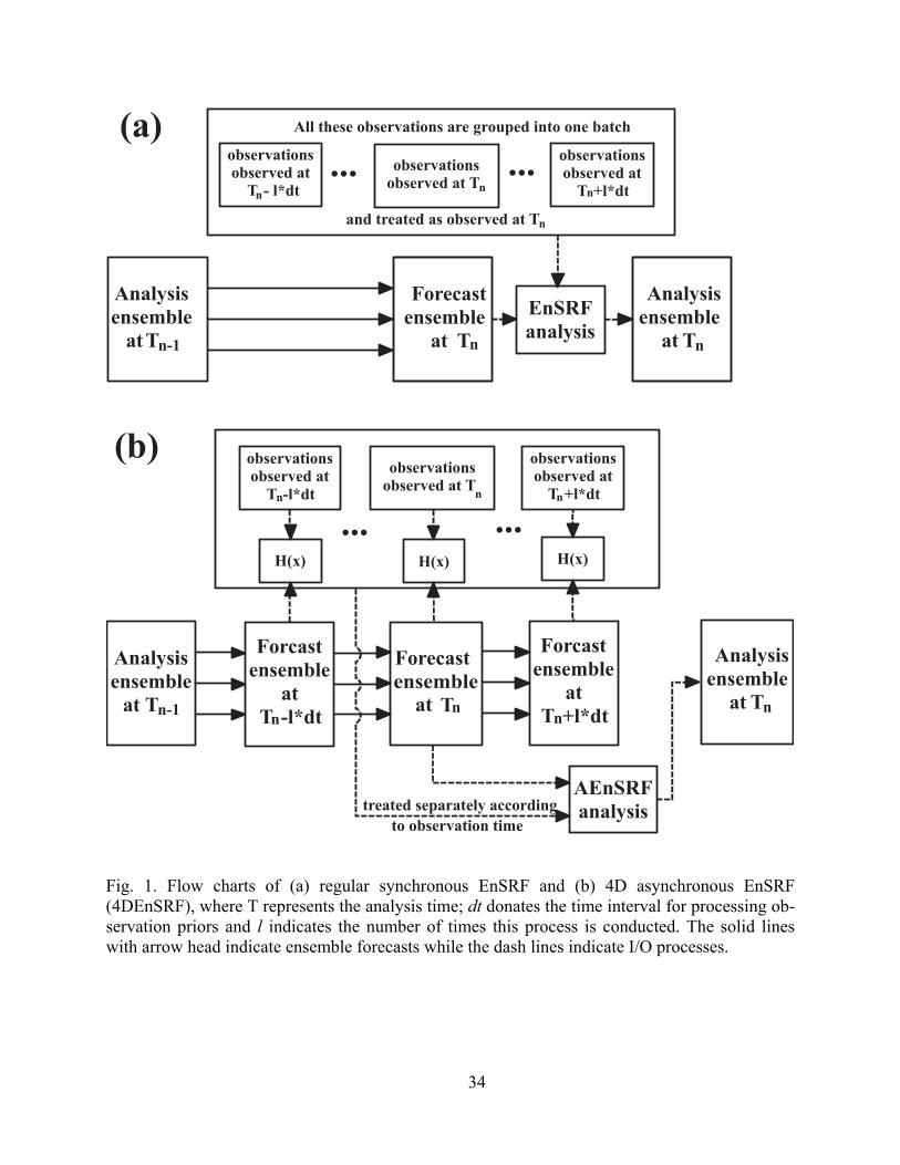
written to the disk. A flow chart of the 4DEnSRF procedure is given in Fig. 1. Compared to the

standard sequential EnSRF where observations are grouped into batches and analyzed at the

analysis times, 4DEnSRF analyzes observations collected at different times of the assimilation

window simultaneously, with observation priors calculated from the background forecast states

at the observation times.

Unlike the cases of 4D-LEnKF (Hunt et al. 2004) and 4D-LETKF (Hunt et al. 2007), the

WH02 EnSRF algorithm on which 4DEnSRF is based analyzes observations one after another.

After an observation is analyzed, the new analysis becomes the background for the next observa-

tion, and typically the prior of the next observation is computed from this new background. In

Eqs. (17) and (18), only model states at the analysis time are updated while at other times obser-

vation priors should be updated by the filter/smoother. Thus it is necessary to write separate

equations for updating these priors, including their ensemble mean and ensemble perturbations

(The observation priors can also be considered part of an extended state vector).

10

For the jth observation, ojy , the update equations for the observation prior ensemble mean,

y , and deviations from the ensemble mean, 'Y , are, respectively:

( )a b o o o bj j jy y y ρ Κ y , (20)

' ' 'a b o o bj j Y Y ρ Κ Y , (21)

where ojΚ is the Kalman gain for the jth observation, with its kth element equal to

, ,1

, ,1

' 'Κ

' ' R

mb bi j i k

o ij,k m

b bi j i j j

i

y y

y y

. (22)

In Eqs. (20) and (21) symbol in the equations represents the Schur (element-wise) product. oρ

is the localization coefficient factor for the observation prior, which in our case is expressed as

= ) / 2o ot s hfρ ρ ρ ρ（ , and the two terms on the right hand side are the static and flow-dependent

parts, respectively. osρ is a spatial localization factor that is specified as a function of the distance

between the observation being processed and the observation prior being updated. tρ is a tem-

poral localization factor that is a function of the time interval between the two observations. For

the flow-dependent part, hfρ , we adopt the hierarchical filter (HF) idea of Anderson (2007) with

hfρ being the regression confidence factor (RCF) of the HF. Equal weight given to the static and

flow-dependent parts was found to work well based on earlier tests. A combination of the static

and flow-dependent parts to form a ‘hybrid’ localization scheme is beneficial because the flow-

dependent part based on the HF is also subject to sampling error.

11

With the above algorithm, for a given observation ojy , priors for those observations with-

in the time window that have not been analyzed are first updated using Eqs. (20) and (21). State

variables are then updated using Eqs. (17) and (18).

Updating the observation priors using the filter is equivalent to updating the model state

then calculating the observation priors from the updated state when the observation operator is

linear. Anderson and Collins (2007) proposed a variant of the serial EnKF that is more friendly

to parallel processing. It pre-computes observation priors in parallel and updates them like state

variables rather than recalculating them from the updated state. Therefore, this variant is referred

to as parallel EnKF (PEnKF). In the case that all data are synchronously observed at the analysis

time, and when our 4DEnSRF also updates observation priors at the analysis time, the 4DEnSRF

and PEnSRF become the same.

Using the most recently updated observation priors and the state ensemble and including

the localization, the state update equations for jth observation are

ˆ ( )a b o aj j jy x x ρ Κ y , (23)

ˆ' ' 'a b aj j X X ρ Κ Y , (24)

where the kth element of Kalman gain ˆjΚ is

, ,1

,

, ,1

' 'Κ̂

' ' R

Nb ai k i j

ij k N

a ai j i j

i

x y

y y

. (25)

Similarly, =( ) / 2t s hfρ ρ ρ ρ in the equations is the localization factor for state variables for a

given observation. The flow-dependent part has the ability to account for movement of features

during the assimilation window. We should point out here that the use of temporal localization

12

will break the formal equivalence between the 4D asynchronous algorithm and the sequential

synchronous algorithm that assimilates data at the observation times, even in the case of perfect

linear model and linear operator; the localization is, however, necessary to alleviate the negative

impact of covariance sampling error especially when the time window is long.

In summary, 4DEnSRF in a single analysis cycle involves three steps: (1) the calculation

of observation priors at the times observations are taken; (2) the update of observation priors;

and (3) the update of model states. These steps are repeated for each observation serially until all

observations in the current time window are processed.

3. OSSE experiments

a. Model configuration and truth simulation

The Weather Research and Forecast (WRF) model V2.2.1 (Skamarock et al. 2005) is

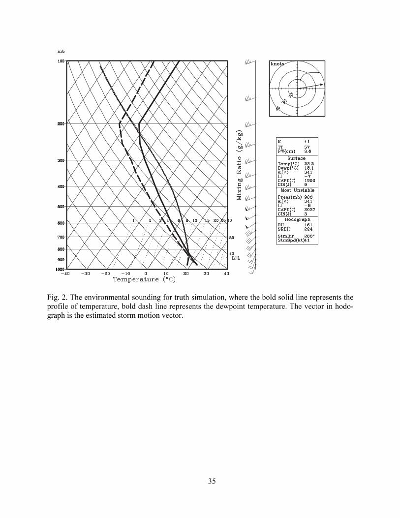
used for the truth simulation and OSSEs. In the truth simulation, a fast-moving, splitting super-

cell storm is simulated, triggered by a thermal bubble in a horizontally homogenous environment.

This environment is defined by a classic Weisman and Klemp (1982) analytic sounding and

shown in Fig. 2. The wind profile is made up of a quarter circle in the lowest 7 km then a straight

westerly hodograph above, plus a uniform (10, 10) m s-1 wind vector added to the entire wind

profile. For all experiments, the domain is 120 km ×120 km × 20 km with 61×61×41 grid

points. The horizontal grid spacing is 2 km and the vertical grid spacing is 0.5 km. A 3 K ellip-

soidal thermal bubble with a horizontal radius of 10 km and a vertical radius of 1.5 km is cen-

tered at x= 10 km, y = 30 km and z = 1.5 km. Other model parameters used include: Runge-Kutta

3rd-order time-integration scheme with a time step of 12 seconds, WRF Single-Moment 6-class

(WSM6) microphysics, and the Rapid Radiative Transfer Model (RRTM) and Dudhia schemes

13

for long and short wave radiation. No cumulus parameterization is included. A 1.5-order turbu-

lent kinetic energy (TKE) closure scheme is used to parameterize subgrid-scale turbulence and a

positive definite scheme is used for the advection of moisture and water variables. Open condi-

tions are used at the lateral boundaries. More details with regard to these parameterization

schemes can be found in Skamarock et al. (2005). The length of simulation is 95 minutes.

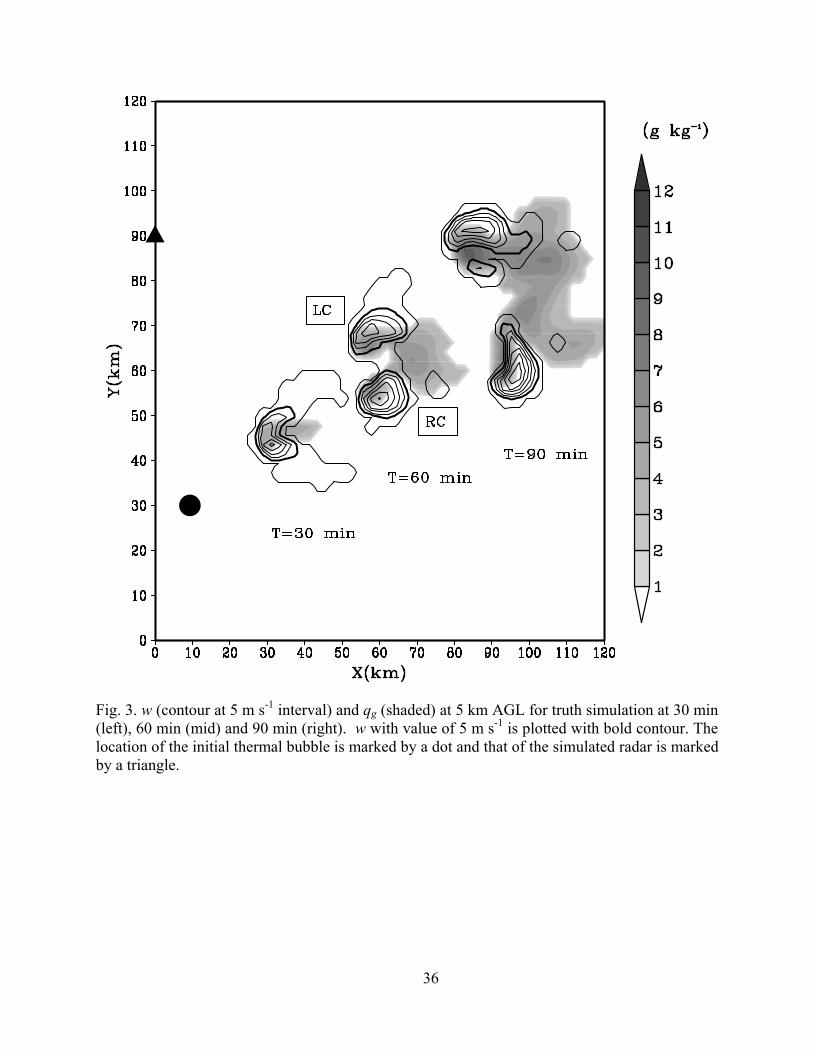
Three stages of the simulated storm are plotted in Fig. 3. At 30 min, the storm is approx-

imately centered at x= 35 km, y = 45 km, about 15 km northeast of its initial location. There are

two updraft maxima in the storm, corresponding to the start of cell splitting. At 60 min, two sep-

arate cells and updraft cores are established and at 5 km AGL the updrafts of the right moving

and left moving cells (hereafter RC and LC) reach about 30 m s-1 and 20 m s-1, respectively. At

90 min, the two cells drift further apart and both remain rather strong. The maximum updraft of

the RC reaches 45 m s-1 during the simulation and its cloud top reaches 15 km AGL.

b. Simulation of radar observations

In this study, observations are simulated for a radar located at x= 0 km, y = 90 km, and its

maximum range is enough to cover the entire model domain. In the vertical, the observations are

simulated on radar elevation levels, as in recent OSSE papers (e.g., Xue et al. 2006; Lei et al.

2007). In the horizontal direction, observations are assumed to be already mapped to the model

grid points, a common practice with radar DA (e.g., Xue et al. 2006). The radar operates in the

standard U.S. WSR-88D volume scan pattern (VCP) 11, which has 14 elevation angles ranging

from 0.5° to 19.5°. Each volume scan spans 5 minutes. Following Yussouf and Stensrud (2010),

the lowest 12 elevations of observations are collected at a rate of 3 elevations per minute and the

upper 2 elevations are collected during the last minute of each volume scan with observations

stored in data files minute-by-minute. Data in each file are assumed to be simultaneously ob-

14

served and these 1 minute data files are referred to as raw data files. The first raw file is at 21

minutes of model time.

Simulated observations are calculated using the observation operators, from model varia-

bles interpolated to the model scalar points in horizontal direction and radar elevations in vertical

direction. For radial velocity rV , the observation operator is

sin)(coscossincos tgggr wwvuV , (26)

where ug, vg and wg represent the model forecast wind components at radar observation points

interpolated from the staggered model grid points, wt represents the terminal fall speed of hy-

drometeors, and θ and ϕ represent the elevation angle and azimuth angle of the radar beam, re-

spectively. For simulated reflectivity Z, the observation operator follows the formulas of Smith et

al. (1975), which are also used in Tong and Xue (2005) and Xue et al. (2006),

)1

(log103610

mmm

ZZZZ hsr

, (27)

where Zr, Zs and Zh are the equivalent reflectivity factors for rainwater, snow and hail, respective-

ly. The reflectivity observation operator in (27) has strong nonlinearity. Random errors drawn

from Gaussian distributions with zero mean and standard deviations of 2 m s-1 and 2 dBZ are

added to radial velocity and reflectivity, respectively. Data are only assimilated where reflectivi-

ty exceeds 10 dBZ, as in earlier OSSE studies (Tong and Xue 2005).

c. Assimilation experiments

In our 4DEnSRF implementation, model variables updated include wind components u,

v, w, geopotential height , potential temperature θ, and the mixing ratios of water vapor qv,

cloud water qc, rain water qr, cloud ice qi, snow qs, and graupel qg. A first guess state is defined

by the environmental sounding used in truth simulation. Random perturbations are added to this

15

initial background to create an initial 40-member ensemble. These random perturbations have a

Gaussian distribution with zero mean and standard deviation of 3 K for θ and 0.5 g kg-1 for qv.

The wind field is not perturbed. The perturbations are smoothed by a recursive filter (e.g., Gao et

al. 2004) with a horizontal correlation scale of 2 km and a vertical correlation scale of 2 model

levels, and are only added at grid points where reflectivity is greater than 10 dBZ. The effect of

this procedure is similar to that used in Tong and Xue (2008) and is computationally more effi-

cient. The relaxation inflation scheme of Zhang et al. (2004) is used to help maintain the ensem-

ble spread, according to

' (1 ) ' 'a a bnew X X X , (30)

where 'anewX is the inflated posterior ensemble, and γ is the weight of background ensemble, set

to 0.5 as in Zhang et al. (2004). Additional inflation is further applied every 5 minutes by scaling

the spread of θ to 2 K in the areas influenced by observational data in the filter updating. A fifth-

order correlation function of Gaspari and Cohn (1999) is used to calculate the localization coeffi-

cients for static localization in both space and time ( osρ and tρ ). The cutoff radii for spatial lo-

calization are 6 km in the horizontal and 2 km in the vertical. For temporal localization, settings

are experiment-dependent and will be given later. In the calculation of RCF hfρ of the hierar-

chical filter, 40 ensemble members are divided into 8 groups of 5 members each.

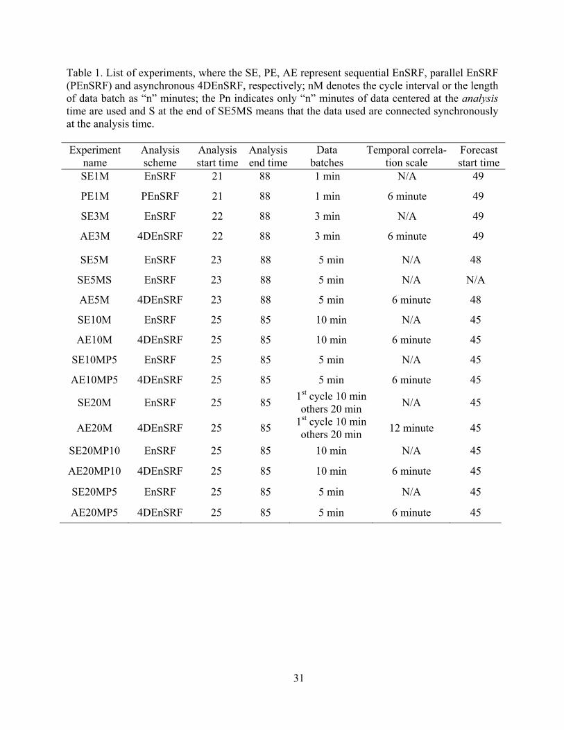
For the purpose of comparison, we design pairs of experiments using 4DEnSRF and

EnSRF respectively. These experiments mostly differ in the data batch lengths (cycle intervals)

which vary from 1 min to 20 min (Table 1). The first two letters in the experiment names indi-

cate the analysis scheme used: SE, AE and PE represent, respectively, synchronous or regular

EnSRF, asynchronous 4DEnSRF, and the Anderson and Collins (2007) parallel EnSRF in which

observation priors at the analysis time are also updated and used in the filter analysis. All non-PE

16

experiments calculate the observation priors at the analysis time from the latest updated state.

The “nM” indicates the cycle interval (data batch length) as “n” minutes. Data batch consists of

data files with times centered on the analysis. For example, in SE1M and PE1M, 1 minute data

batches valid at the analysis time are used; the pair examines the effects of nonlinear radial ve-

locity (because of the involvement of terminal velocity wt) and reflectivity observation operators

in PEnSRF versus regular EnSRF. As discussed in Section 2c, when all data are synchronously

observed, PEnSRF is equivalent to 4DEnSRF, therefore AE1M would be the same as PE1M. In

SE3M, raw data files 1 minute before and after the analysis time are assumed to be valid at the

analysis time while in AE3M they are used at their valid times. Similarly for other experiments

with longer batch lengths. Here, we choose to update model state at the middle of the assimila-

tion window to minimize the temporal sampling error. In a nonlinear system, the closer are the

observations to the analysis time, the better is the linear approximation.

In addition, “P” in the experiment name indicates that only partial data are used. The

number following “P” represents the time interval of data used. For instance, “P10” means 10

minutes of data centered at the analysis time are used in each cycle. The “S” at the end of

SE5MS means that the data are actually synchronous, created from the truth simulation at the

instance of analysis. This is the case in SE5MS only, which is designed to measure the impact of

data timing error only on EnSRF analysis. In all experiments, we perform the first analysis at 21

to 25 minutes (depending on the cycle length), run the analysis cycles until 85 to 88 minutes, and

launch a deterministic forecast from the ensemble mean analysis at about 45 minutes. No fore-

cast is launched for SE5MS. In AE20M and SE20M, 20 minute data batch is not valid at 25

minutes so for the first cycle a 10 minute data batch is used.

4. Results and discussions

17

To simplify the presentation, the square root of mean difference total energy (DTE) is

used to evaluate the performance of assimilation algorithm:

2 2 2 21DTE ( ) ( ) ( ) ( )

2p

r

Cu v w

T

, (31)

where denotes the difference of the ensemble mean from the truth, 1 11004.7J kg KpC is

the specific heat of dry air at constant pressure, and Tr = 270 K is the reference temperature. We

added vertical velocity w compared to the DTE used in (Meng and Zhang 2007). Furthermore, to

evaluate errors in moisture and hydrometer fields, we define

2 2 2 21HydroDTE ( ) ( ) ( ) ( )

2 v r s gq q q q , (32)

where vq , rq , sq and gq are the mixing ratios of water vapor, rain water, snow and graupel,

respectively. Similar to previous radar OSSE studies (e.g., Tong and Xue 2005; Xue et al. 2006),

DTE and HydroDTE diagnostics are calculated only at grid points where the truth reflectivity

exceeds 10 dBZ. Meanwhile, we refer the square root of mean DTE and HydroDTE as RM_DTE

and RM_HydroDTE for convenience.

a. High frequency (1 and 3 minute) assimilation experiments

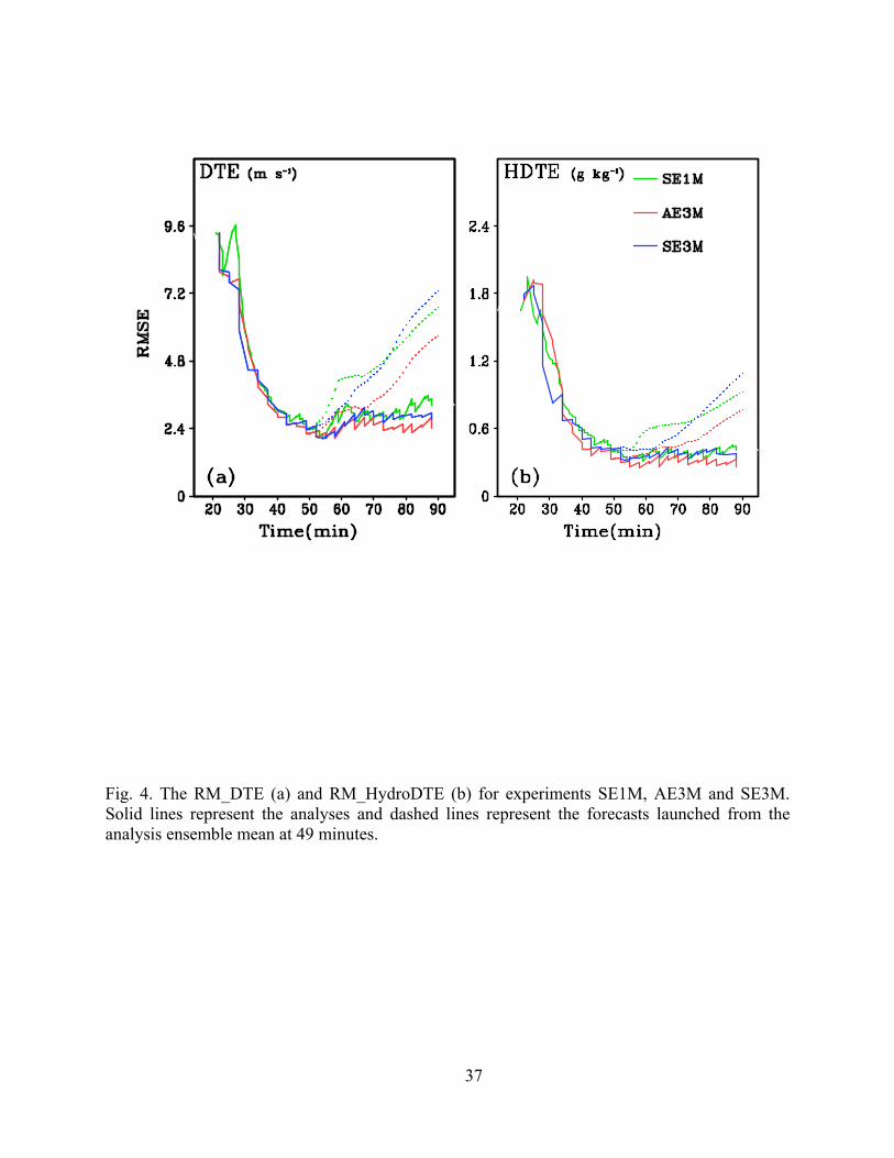
We first look at the results using 1 minute update cycles or data batches. The analysis

RM_DTE and RM_HydroDTE obtained in PE1M are found to be very close to those of SE1M

throughout the assimilation. The differences between final analysis errors in PE1M and SE1M

are about 0.3 m s-1 and 0.08 g kg-1 for RM_DTE and RM_HydroDTE, respectively. Therefore,

only the RM_DTE and RM_HydroDTE for SE1M are plotted in Fig. 4. Also, the forecast from

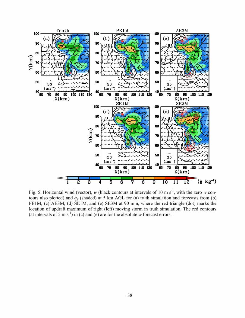
PEnSRF analysis is similar to that from EnSRF analysis. In Fig. 5, it can be seen that the loca-

tions of forecast updraft cores in PE1M and SE1M are very close to the truth for both LC and RC,

18

with the position errors being less than 2 km in both experiments. The updraft maxima in both

experiments reach 30 m s-1 and 20 m s-1 for RC and LC respectively, capturing the updraft

strength well. These results suggest that the way updated observation priors are obtained (the on-

ly difference between the two experiments) does not affect the results much in our case even

though nonlinearity exists with the reflectivity and radial velocity operators.

Next, we compare the results between slightly longer 3 min cycle length experiments. It

can be seen in Fig. 4 that the analysis RM_DTE and RM_HydroDTE for SE3M and AE3M are

mostly similar to each other; however, there are two clear differences. One is that the

RM_HydroDTE is reduced more slowly in AE3M than that in SE3M before 30 min. This is like-

ly caused by the highly nonlinear model, because Eqs. (13) and (14) are only strictly valid when

model is linear. Poor quality temporal covariance used in AE3M during the earlier cycles can be

another reason. Another difference is that the analysis error in AE3M becomes smaller than that

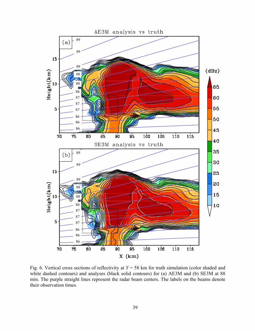
in SE3M in later cycles. In Fig. 6, it can be seen that the 4DEnSRF analysis at 88 min matches

well the truth at all levels while the EnSRF analysis is not as good, especially within the dashed

rectangle. In this area, the EnSRF analyzed fields lag behind (displaced to the west of) the truth

fields. The radar beams plotted in Fig. 6 indicate that the analysis in this area is produced using

data observed at 87 min, which is one minute earlier than the analysis time. Due to this timing

error, spatial displacement error results in the EnSRF analysis for this moving storm (the storm

movement speed is about 21 m s-1 in this period). When a deterministic forecast is launched from

the analysis, the forecast error in AE3M is clearly smaller than that in SE3M. In Fig. 5, even

though the forecast storms in AE3M and SE3M look qualitatively similar, the w errors (red con-

tours) are larger in SE3M (Fig. 5e). In the RC region, w error exceeds 20 m s-1 in SE3M while

that in AE3M is less than 10 m s-1. The location errors with the updraft cores are also smaller

19

with AE3M. These results indicate that even for a short 3 minute cycle length, the asynchronous

formation still improves the storm analysis and forecast.

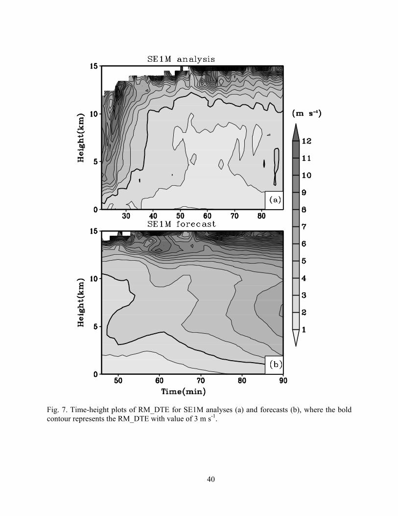
We now go back to experiment SE1M to see if the short 1 minute cycle length is benefi-

cial. Fig. 4 shows that the minimum analysis errors are reached at around 55 min in all three ex-

periments; after that time, the errors remain level or increase somewhat, especially in SE1M. The

analysis RM_DTE in SE1M increases to 3.2 m s-1 at 88 min compared to 2.1 m s-1 at 55 min, and

among the three experiments the errors of SE1M are actually the largest at the end of assimila-

tion window. We believe this is at least partially caused by the analysis of incomplete volumes of

data, 2 to 3 elevations at a time, when using 1 minute cycles. Doing so has a tendency to intro-

duce spatial discontinuity and hence imbalance in the model state. Evidence can be seen in Fig.

7a that the error at upper levels is large (over 10 m s-1), accompanied with wavelike fluctuations

having periods of 3-5 minutes, roughly matching the intervals at which radar observations at the-

se levels are introduced into the system. The problem is more significant at the upper levels be-

cause the vertical resolution of observations is lower, and as a result the high frequency gravity

wave oscillations in the stratosphere are more difficult to analyze accurately from radar data.

Another reason for the increased error level is the frequent stopping and restarting of the WRF

model. Even without the assimilation of any data, a restart of a WRF run using its ‘cold start’

input file does not exactly reproduce the forecast of an otherwise non-stop run. It is because the

WRF stores some state variables and diagnoses others, causing (small) differences in the model

state after restart (such small differences are generally inevitable with typical weather models

unless restart files with a full state dump are used). Fig. 7b shows that the forecast error grows in

time with a signature of downward error propagation. These results indicate that there is addi-

tional benefit of doing 4D asynchronous EnKF, even when computational cost is not an issue.

20

b. Assimilation experiments with longer cycle lengths

In this section, we compare the performance of 4DEnSRF and EnSRF with longer cycle

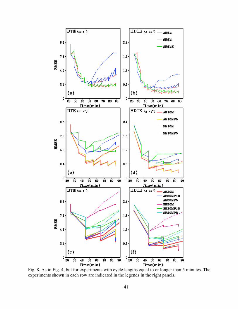
lengths. We first compare SE5M and AE5M, for which RM_DTE and RM_HydroDTE are plot-

ted in Fig. 8. From Fig. 8a,b, we can see that 4DEnSRF performs worse than EnSRF in the early

cycles but become much better later on (after 50 min or 6 cycles). At the end of assimilation, the

analysis errors in AE5M are only half as large as those in SE5M for both RM_DTE and

RM_HydroDTE. Similar behaviors were also observed earlier with SE3M and AE3M. Poor

quality temporal covariance and model nonlinearity are suspected to be the causes. In other

words, during the earlier cycles when the state estimation and associated covariance is poor, data

timing error in the regular EnSRF is secondary. Fortunately, as the state estimation improves,

the asynchronous 4DEnSRF becomes superior (Fig. 8a,b).

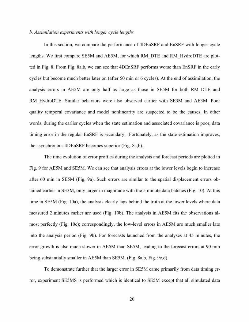
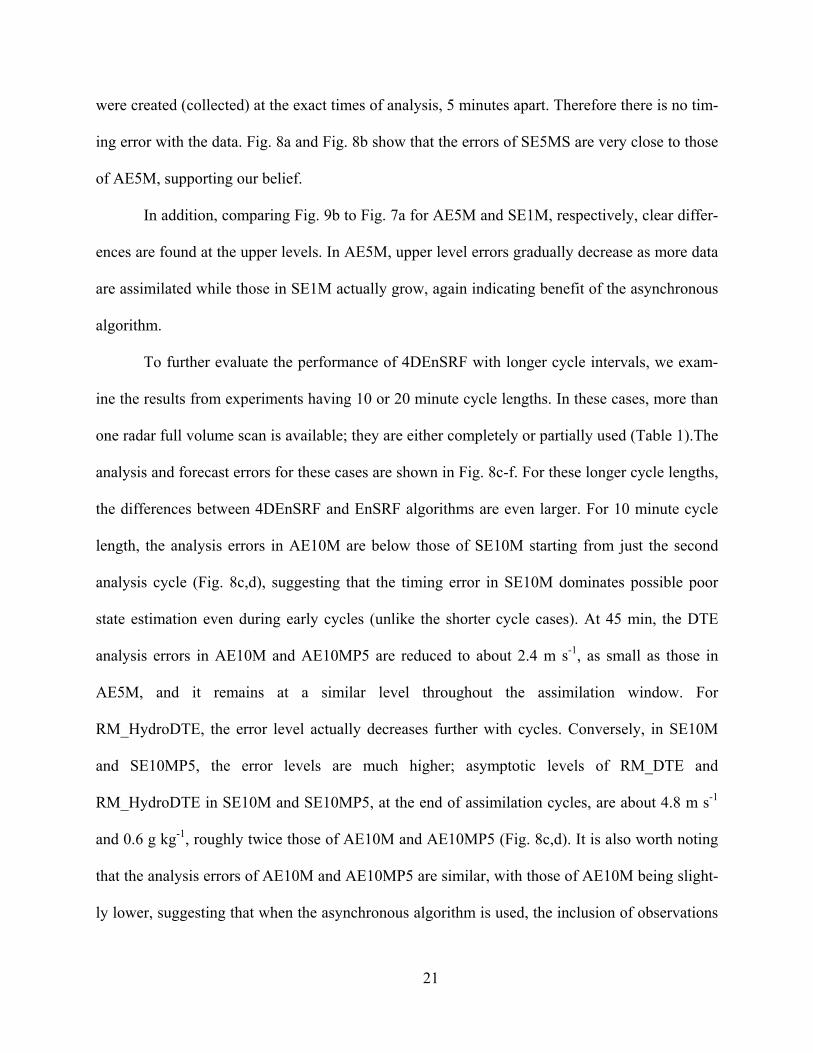
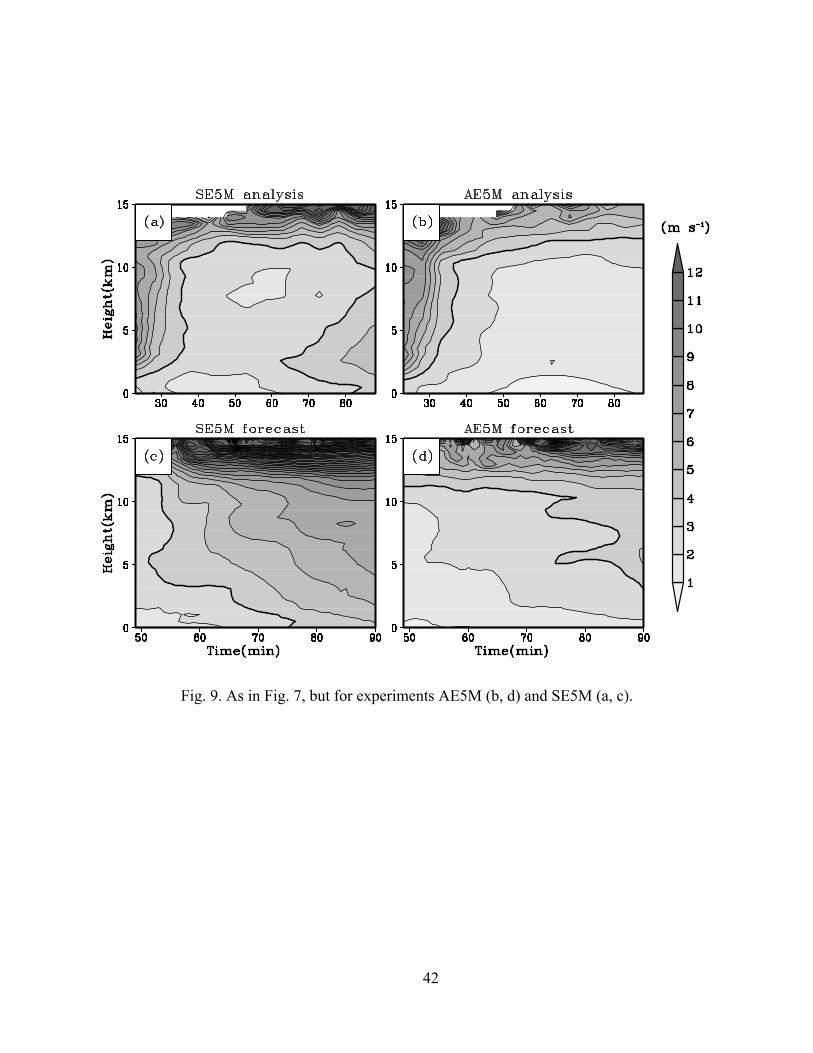
The time evolution of error profiles during the analysis and forecast periods are plotted in

Fig. 9 for AE5M and SE5M. We can see that analysis errors at the lower levels begin to increase

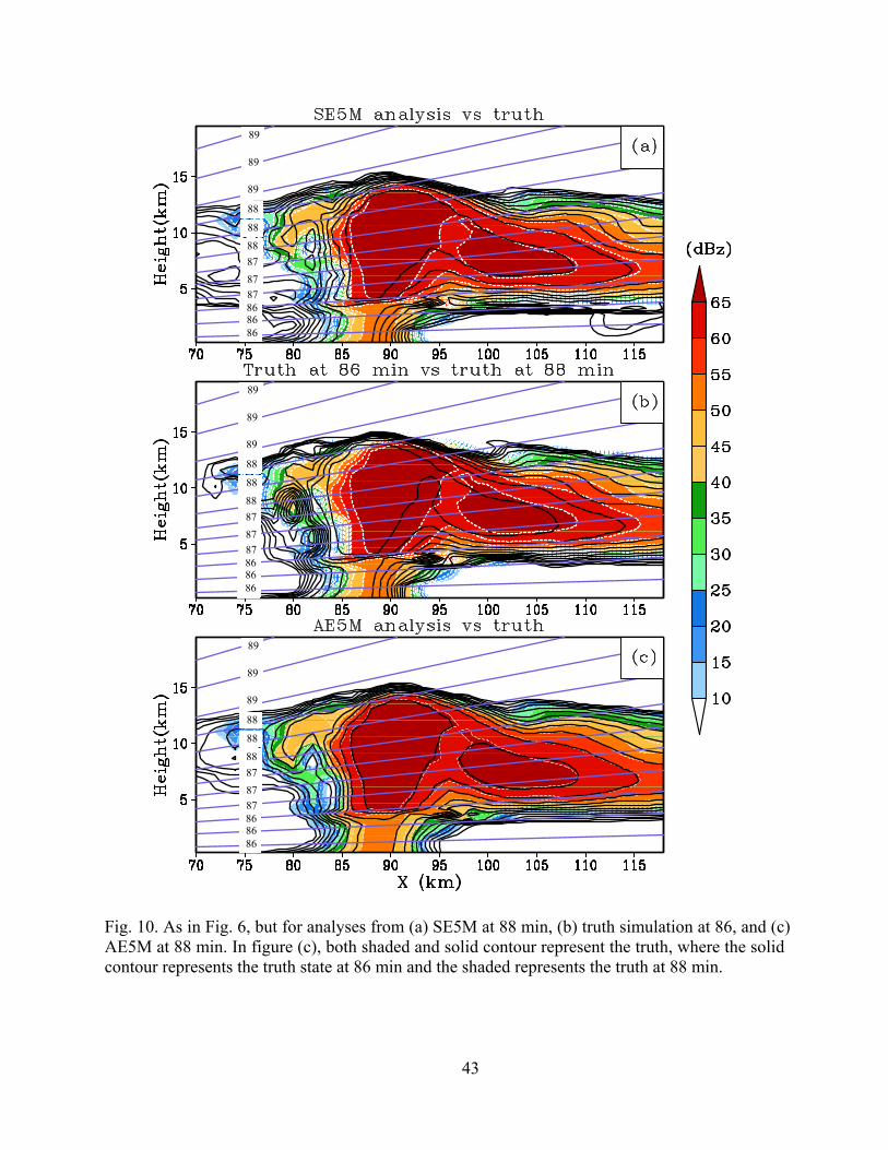
after 60 min in SE5M (Fig. 9a). Such errors are similar to the spatial displacement errors ob-

tained earlier in SE3M, only larger in magnitude with the 5 minute data batches (Fig. 10). At this

time in SE5M (Fig. 10a), the analysis clearly lags behind the truth at the lower levels where data

measured 2 minutes earlier are used (Fig. 10b). The analysis in AE5M fits the observations al-

most perfectly (Fig. 10c); correspondingly, the low-level errors in AE5M are much smaller late

into the analysis period (Fig. 9b). For forecasts launched from the analyses at 45 minutes, the

error growth is also much slower in AE5M than SE5M, leading to the forecast errors at 90 min

being substantially smaller in AE5M than SE5M. (Fig. 8a,b, Fig. 9c,d).

To demonstrate further that the larger error in SE5M came primarily from data timing er-

ror, experiment SE5MS is performed which is identical to SE5M except that all simulated data

21

were created (collected) at the exact times of analysis, 5 minutes apart. Therefore there is no tim-

ing error with the data. Fig. 8a and Fig. 8b show that the errors of SE5MS are very close to those

of AE5M, supporting our belief.

In addition, comparing Fig. 9b to Fig. 7a for AE5M and SE1M, respectively, clear differ-

ences are found at the upper levels. In AE5M, upper level errors gradually decrease as more data

are assimilated while those in SE1M actually grow, again indicating benefit of the asynchronous

algorithm.

To further evaluate the performance of 4DEnSRF with longer cycle intervals, we exam-

ine the results from experiments having 10 or 20 minute cycle lengths. In these cases, more than

one radar full volume scan is available; they are either completely or partially used (Table 1).The

analysis and forecast errors for these cases are shown in Fig. 8c-f. For these longer cycle lengths,

the differences between 4DEnSRF and EnSRF algorithms are even larger. For 10 minute cycle

length, the analysis errors in AE10M are below those of SE10M starting from just the second

analysis cycle (Fig. 8c,d), suggesting that the timing error in SE10M dominates possible poor

state estimation even during early cycles (unlike the shorter cycle cases). At 45 min, the DTE

analysis errors in AE10M and AE10MP5 are reduced to about 2.4 m s-1, as small as those in

AE5M, and it remains at a similar level throughout the assimilation window. For

RM_HydroDTE, the error level actually decreases further with cycles. Conversely, in SE10M

and SE10MP5, the error levels are much higher; asymptotic levels of RM_DTE and

RM_HydroDTE in SE10M and SE10MP5, at the end of assimilation cycles, are about 4.8 m s-1

and 0.6 g kg-1, roughly twice those of AE10M and AE10MP5 (Fig. 8c,d). It is also worth noting

that the analysis errors of AE10M and AE10MP5 are similar, with those of AE10M being slight-

ly lower, suggesting that when the asynchronous algorithm is used, the inclusion of observations

22

beyond one volume scan interval can help the analysis (at least does not hurt). On the other hand,

the errors at the end of the assimilation cycles are higher in SE10M compared to SE10MP5, in-

dicating that the inclusion of additional data with larger timing error can actually hurt the analy-

sis.

Due to the smaller analysis errors, the errors of forecasts launched at 45 min are also

smaller in AE10M and AE10MP5 than those in SE10M and SE10MP5 throughout the forecast

period (Fig. 8c,d). This advantage of the 4D asynchronous algorithm becomes even larger when

the cycle length is extended to 20 min. Fig. 8e and Fig. 8f show that among all experiments with

a 20 min cycle length, AE20M produces the lowest analysis and forecast errors while SE20M

has the highest error levels. The differences in error are due, once again, to the large data timing

errors that can occur in a 20-minute cycle window. For such long cycle lengths, discarding data

with large timing errors aids the regular EnSRF, as errors of SE20MP10 are lower than those of

SE20M and errors of SE20MP5 are even lower. Note that the differences between SE20M and

SE20MP10 are larger than those between SE20MP10 and SE20MP5 (Fig. 8e,f). The errors of

SE20MP5 are still higher than those of each asynchronous experiment. It is worth noting further

that the analysis errors in AE20M during the later cycles are not much higher than those of

AE10M or even AE5M, which is important due to the associated computational savings using

longer intervals.

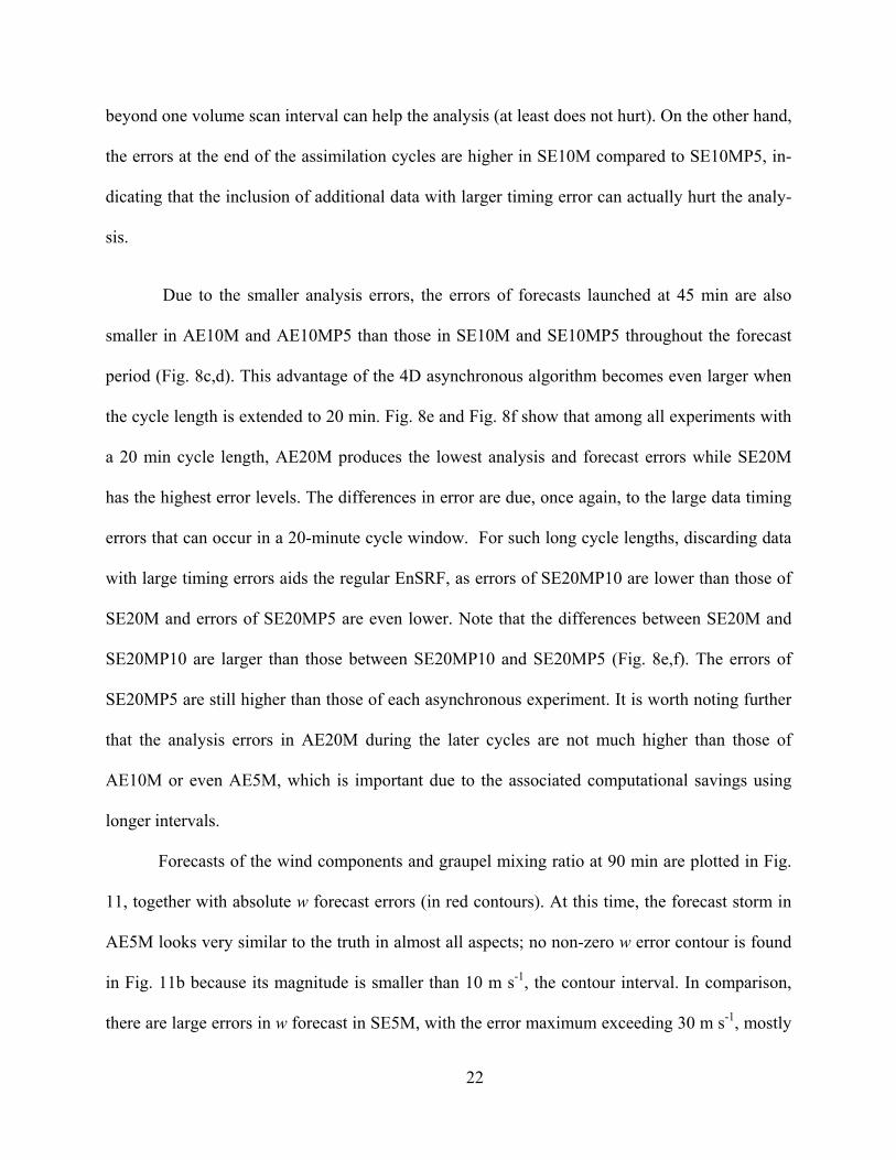
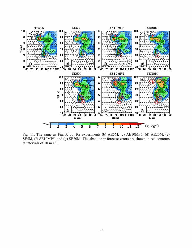
Forecasts of the wind components and graupel mixing ratio at 90 min are plotted in Fig.

11, together with absolute w forecast errors (in red contours). At this time, the forecast storm in

AE5M looks very similar to the truth in almost all aspects; no non-zero w error contour is found

in Fig. 11b because its magnitude is smaller than 10 m s-1, the contour interval. In comparison,

there are large errors in w forecast in SE5M, with the error maximum exceeding 30 m s-1, mostly

23

associated with the lagging spatial displacement error with RC. This is consistent with the large

errors at the end of the forecast in Figs. 8a,b. As the cycle length increases, the differences be-

tween 4DEnSRF and EnSRF become more evident. The northern cell in the forecasts of

AE10MP5 and AE20M matches the truth well, with the absolute w forecast error being less than

10 m s-1. In contrast, the errors associated with LC are much larger in SE10MP5 and SE20M in

both graupel and w forecast fields, with the absolute w forecast error exceeding 10 m s-1 and 20

m s-1 in them, respectively. The updraft of the northern cell is mostly missing in SE20M (Fig.

11g). Similar differences can also be found with the southern cell, but more significant. Overall,

the forecast storm pattern is clearly the worst in SE20M. The comparisons again confirm the

benefit of 4DEnSRF over the regular EnSRF when assimilating frequent radar data using a cycle

length 5 minutes or longer.

5. Summary and conclusions

In this study, a 4D ensemble square root filter algorithm (4DEnSRF) is proposed for as-

similating high-frequency asynchronous observations, such as those from weather radars. Given

the serial nature of EnSRF, the 4DEnSRF algorithm pre-calculates observation priors from en-

semble model states at observation times and updates the observation priors at asynchronous ob-

servational times to their posteriors using the filter; these posteriors, or the most recently updated

observation priors, are used to update model state variables at the analysis time. Such an algo-

rithm has the benefit of being able to utilize more observations collected over time using fewer

analysis cycles, thereby reducing computational costs and potentially improving filter perfor-

mance also. In our current 4DEnSRF implementation, a hybrid approach that combines static

spatiotemporal localization with adaptive localization based on the hierarchical ensemble filter

24

idea of Anderson (2007) is employed; the latter is in principle able to take into account system

movement when localizing spatial covariances involving time shift.

We tested the 4DEnSRF using simulated data from a single Doppler radar for a supercell

storm. The radar data are simulated elevation by elevation and are grouped into data batches with

different time intervals and assimilated with analysis cycles of the same lengths. Parallel sets of

experiments using 4DEnSRF and the regular EnSRF are performed to compare their perfor-

mance. Data batch or cycle lengths between 1 and 20 minutes are examined. EnSRF always as-

sumes that all data used in a given cycle are valid at the same analysis time. When the cycle

length is 10 or 20 min, some experiments use only data taken within a 5 or 10 minute time win-

dow centered on the analysis time.

It is shown through OSSEs that 4DEnSRF performs better than EnSRF when the cycle

length is 3 minutes or longer. Observation timing error is the main cause of the poorer perfor-

mance of EnSRF for the analyses and for forecasts launched half way through the assimilation

cycles; the longer is the cycle length, the large is the difference. For long cycle lengths,

4DEnSRF produces better analyses when utilizing all data at their correct times within the cycle

window, but for EnSRF discarding data far away from the analysis time yields better analyses

than using all data (that have timing error). Assimilating only a couple of elevations at a time us-

ing very short (~1 minute) cycles with regular EnSRF tends to introduce imbalances into the

model state that degrades the subsequent analyses and forecasts.

More specifically, when the assimilation cycles are 3 minute long, the 4DEnSRF analysis

errors are smaller than those of EnSRF after first few analysis cycles. The increase error level in

EnSRF was shown to be mostly related to the spatial displacement error of features that have

moved between the times radar measurements were taken and the times at which such data are

25

assimilated. This timing error in EnSRF comes from the assumption that all data were valid at

the analysis time. The 4DEnSRF correctly uses the measurements at the times they were taken.

The results with 5 minute cycle length were similar; although the differences between 4DEnSRF

and EnSRF analyses and forecasts were somewhat larger.

When cycle interval is increased to 10 minutes or 20 minutes, the advantage of using

4DEnSRF becomes even more evident. In these cases, the impact of timing error dominates over

other issues with the filters. With 4DEnSRF, the filter is able to reduce the analysis errors to lev-

els close to those obtained using 5 minute cycle length even when a 20-minute cycle length is

used, while the error levels of the corresponding EnSRF analyses are about twice as large. The

large error differences are also maintained in the forecasts launched from analyses midway

through the analysis cycles.

Based on the OSSE results, several conclusions can be drawn, i) the ‘parallel’ EnSRF al-

gorithm that updates observation priors at the analysis time as part of the extended state vector

performs comparably with regular EnSRF when tested with 1 minute data batches/cycle length

(hence data timing error is negligible); ii) in the presence of data timing error with regular

EnSRF, 4DEnSRF works better than EnSRF; iii) the advantage of 4DEnSRF becomes larger as

the cycle increases, especially when the data span more than one radar volume scan interval; iv)

very short assimilation intervals (~1 minute) can introduce shock and imbalance into the model

state that degrade the analysis and forecast; v) when the assimilation cycle spans more than one

volume scan, it is better for the regular EnSRF to use only the data from the closest scan volume

to reduce the impact of timing errors in the data while for 4DEnSRF using all data yields better

results; vi) overall, using 4DEnSRF with 5 to 10 minute cycle lengths yields the best results for

our test problem but the final analysis errors using a 20 min cycle length are only slightly larger.

26

Considering the significant computational cost saving, the use of the 4D algorithm with ~20 mi-

nute cycles is attractive, especially for realtime applications. The 4DEnSRF algorithm has also

been implemented in the full EnKF framework of the ARPS model with embedded (within the

model) observation prior calculations. The system is being tested with real radar data and the re-

sults will be reported in a future paper.

Acknowledgments: This work was primarily supported by NSF grant OCI-0905040, AGS-

0802888, NOAA Warn-on-Forecast Project under NA080AR4320904, and grant KLME060203

from NUIST. Partial support was also provided by NSF AGS-0750790, AGS-0941491, AGS-

1046171, and AGS-1046081. J. Min was also supported by Meteorology Commonwealth Project

of China (GYHY200806029) and the Cultivation Fund of the Key Scientific and Technical In-

novation Project，Ministry of Education of China (No: 708051). Discussions with CAPS scien-

tists, including Dr. Youngsun Jung and Robin Tanamachi, had been beneficial. Computations

were carried out at the University of Oklahoma Supercomputer Center for Education and Re-

search (OSCER), and on the CAPS Linux Cluster machines. Nicholas Gasperoni is thanked for

proofreading the manuscript. Comments by Dr. Pavel Sakov and an anonymous reviewer im-

proved the manuscript.

27

References

Anderson JL, 2007. Exploring the need for localization in ensemble data assimilation using a

hierarchical ensemble filter. Physica D, 230: 99-111.

Anderson JL, Collins N, 2007. Scalable implementations of ensemble filter algorithms for data

assimilation. J. Atmos. Oceanic Technol., 24: 1452-1463.

Compo GP, Whitaker JS, Sardeshmukh PD, Matsui N, Allan RJ, Yin X, Gleason BE, Vose RS,

Rutledge G, Bessemoulin P, Bronnimann S, Brunet M, Crouthamel RI, Grant AN,

Groisman PY, Jones PD, Kruk MC, Kruger AC, Marshall GJ, Maugeri M, Mok HY,

Nordli O, Ross TF, Trigo RM, Wang XL, Woodruff SD, Worley SJ, 2011. The Twentieth

Century Reanalysis Project. Quart. J. Roy. Meteor. Soc., 137: 1-28.

Dowell DC, Wicker LJ, 2009. Additive Noise for Storm-Scale Ensemble Data Assimilation. J.

Atmos. Oceanic Technol., 26: 911-927.

Evensen G, 1994. Sequential data assimilation with a nonlinear quasi-geostrophic model using

Monte Carlo methods to forecast error statistics. J. Geophys. Res., 99: 10143-10162.

Evensen G, 2003. The ensemble Kalman filter: Theoretical formulation and practical

implementation. Ocean Dynamics, 53: 343-367.

Evensen G, van Leeuwen PJ, 2000. An ensemble Kalman smoother for nonlinear dynamics. Mon.

Wea. Rev., 128: 1852-1867.

Gao J-D, Xue M, Brewster K, Droegemeier KK, 2004. A three-dimensional variational data

analysis method with recursive filter for Doppler radars. J. Atmos. Ocean. Tech., 21: 457-

469.

Gaspari G, Cohn SE, 1999. Construction of correlation functions in two and three dimensions.

Quart. J. Roy. Meteor. Soc., 125: 723-757.

28

Hu M, Xue M, 2007. Impact of configurations of rapid intermittent assimilation of WSR-88D

radar data for the 8 May 2003 Oklahoma City tornadic thunderstorm case. Mon. Wea.

Rev., 135: 507–525.

Hunt BR, Kostelich EJ, Szunyogh I, 2007. Efficient data assimilation for spatiotemporal chaos:

A local ensemble transform Kalman filter. Physica D, 230: 112-126.

Hunt BR, Kalnay E, Kostelich EJ, Ott E, Patil DJ, Sauer T, Szunyogh I, Yorke JA, Zimin AV,

2004. Four-dimensional ensemble Kalman filtering. Tellus, 56: 273-277.

Lei T, Xue M, Yu T, Teshiba M, 2007: Study on the optimal scanning strategies of phase-array

radar through ensemble Kalman filter assimilation of simulated data. 33rd Int. Conf.

Radar Meteor., Cairns, Australia, Amer. Meteor. Soc., CDROM P7.1.

Lorenz EN, 1996: Predictability: a problem partly solved. Proceedings of the Seminar on

Predictability, ECMWF, 40-58.

Meng ZY, Zhang FQ, 2007. Tests of an ensemble Kalman filter for mesoscale and regional-scale

data assimilation. Part II: Imperfect model experiments. Mon. Wea. Rev., 135: 1403-1423.

Sakov P, Evensen G, Bertino L, 2010. Asynchronous data assimilation with the EnKF. Tellus, 62:

24-29.

Skamarock WC, Klemp JB, Dudhia J, Gill D, Barker D, Wang W, Powers JG, 2005: A

description of the Advanced Research WRF Version 2. NCAR Technical Note

NCAR/TN-468+STR.

Smith PL, Jr., Myers CG, Orville HD, 1975. Radar reflectivity factor calculations in numerical

cloud models using bulk parameterization of precipitation processes. J. Appl. Meteor., 14:

1156-1165.

29

Snook N, Xue M, Jung J, 2011. Analysis of a tornadic meoscale convective vortex based on

ensemble Kalman filter assimilation of CASA X-band and WSR-88D radar data. Mon.

Wea. Rev., 139: 3446-3468.

Snyder C, Zhang F, 2003. Assimilation of simulated Doppler radar observations with an

ensemble Kalman filter. Mon. Wea. Rev., 131: 1663-1677.

Tong M, Xue M, 2008. Simultaneous estimation of microphysical parameters and atmospheric

state with radar data and ensemble square-root Kalman filter. Part II: Parameter

estimation experiments. Mon. Wea. Rev., 136: 1649–1668.

Tong MJ, Xue M, 2005. Ensemble Kalman filter assimilation of Doppler radar data with a

compressible nonhydrostatic model: OSS experiments. Mon. Wea. Rev., 133: 1789-1807.

Weisman ML, Klemp JB, 1982. The dependence of numerically simulated convective storms on

vertical wind shear and buoyancy. Mon. Wea. Rev., 110: 504-520.

Whitaker JS, Hamill TM, 2002. Ensemble data assimilation without perturbed observations. Mon.

Wea. Rev., 130: 1913-1924.

Xue M, Tong M, Droegemeier KK, 2006. An OSSE framework based on the ensemble square-

root Kalman filter for evaluating impact of data from radar networks on thunderstorm

analysis and forecast. J. Atmos. Ocean Tech., 23: 46–66.

Xue M, Wang D-H, Gao J-D, Brewster K, Droegemeier KK, 2003. The Advanced Regional

Prediction System (ARPS), storm-scale numerical weather prediction and data

assimilation. Meteor. Atmos. Physics, 82: 139-170.

Yang SC, Kalnay E, Hunt B, Bowler NE, 2009. Weight interpolation for efficient data

assimilation with the Local Ensemble Transform Kalman Filter. Quart. J. Roy. Meteor.

Soc., 135: 251-262.

30

Yussouf N, Stensrud DJ, 2010. Impact of Phased-Array Radar Observations over a Short

Assimilation Period: Observing System Simulation Experiments Using an Ensemble

Kalman Filter. Mon. Wea. Rev., 138: 517-538.

Zhang F, Snyder C, Sun J, 2004. Impacts of initial estimate and observations on the convective-

scale data assimilation with an ensemble Kalman filter. Mon. Wea. Rev., 132: 1238-1253.

Zhang F, Weng Y, Sippel JA, Meng Z, Bishop CH, 2009. Cloud-resolving hurricane

initialization and prediction through assimilation of Dopple radar observations with an

ensemble Kalman filter. Mon. Wea. Rev., 137: 2105-2125.

31

Table 1. List of experiments, where the SE, PE, AE represent sequential EnSRF, parallel EnSRF (PEnSRF) and asynchronous 4DEnSRF, respectively; nM denotes the cycle interval or the length of data batch as “n” minutes; the Pn indicates only “n” minutes of data centered at the analysis time are used and S at the end of SE5MS means that the data used are connected synchronously at the analysis time.

Experiment

name Analysis scheme

Analysis start time

Analysis end time

Data batches

Temporal correla-tion scale

Forecast start time

SE1M EnSRF 21 88 1 min N/A 49

PE1M PEnSRF 21 88 1 min 6 minute 49

SE3M EnSRF 22 88 3 min N/A 49

AE3M 4DEnSRF 22 88 3 min 6 minute 49

SE5M EnSRF 23 88 5 min N/A 48

SE5MS EnSRF 23 88 5 min N/A N/A

AE5M 4DEnSRF 23 88 5 min 6 minute 48

SE10M EnSRF 25 85 10 min N/A 45

AE10M 4DEnSRF 25 85 10 min 6 minute 45

SE10MP5 EnSRF 25 85 5 min N/A 45

AE10MP5 4DEnSRF 25 85 5 min 6 minute 45

SE20M EnSRF 25 85 1st cycle 10 min others 20 min

N/A 45

AE20M 4DEnSRF 25 85 1st cycle 10 min others 20 min

12 minute 45

SE20MP10 EnSRF 25 85 10 min N/A 45

AE20MP10 4DEnSRF 25 85 10 min 6 minute 45

SE20MP5 EnSRF 25 85 5 min N/A 45

AE20MP5 4DEnSRF 25 85 5 min 6 minute 45

32

List of figures

Fig. 1. Flow charts of (a) regular synchronous EnSRF and (b) 4D asynchronous EnSRF

(4DEnSRF), where T represents the analysis time; dt donates the time interval for

processing observation priors and l indicates the number of times this process is

conducted. The solid lines with arrow head indicate ensemble forecasts while the dash

lines indicate I/O processes. 

Fig. 2. The environmental sounding for truth simulation, where the bold solid line represents the

profile of temperature, bold dash line represents the dewpoint temperature. The vector in

hodograph is the estimated storm motion vector. 

Fig. 3. w (contour at 5 m s-1 interval) and qg (shaded) at 5 km AGL for truth simulation at 30 min

(left), 60 min (mid) and 90 min (right). w with value of 5 m s-1 is plotted with bold

contour. The location of the initial thermal bubble is marked by a dot and that of the

simulated radar is marked by a triangle. 

Fig. 4. The RM_DTE (a) and RM_HydroDTE (b) for experiments SE1M, AE3M and SE3M.

Solid lines represent the analyses and dashed lines represent the forecasts launched from

the analysis ensemble mean at 49 minutes. 

Fig. 5. Horizontal wind (vector), w (black contours at intervals of 10 m s-1, with the zero w

contours also plotted) and qg (shaded) at 5 km AGL for (a) truth simulation and forecasts

from (b) PE1M, (c) AE3M, (d) SE1M, and (e) SE3M at 90 min, where the red triangle

(dot) marks the location of updraft maximum of right (left) moving storm in truth

simulation. The red contours (at intervals of 5 m s-1) in (c) and (e) are for the absolute w

forecast errors. 

33

Fig. 6. Vertical cross sections of reflectivity at Y = 58 km for truth simulation (color shaded and

white dashed contours) and analyses (black solid contours) for (a) AE3M and (b) SE3M

at 88 min. The purple straight lines represent the radar beam centers. The labels on the

beams denote their observation times. 

Fig. 7. Time-height plots of RM_DTE for SE1M analyses (a) and forecasts (b), where the bold

contour represents the RM_DTE with value of 3 m s-1. 

Fig. 8. As in Fig. 4, but for experiments with cycle lengths equal to or longer than 5 minutes. The

experiments shown in each row are indicated in the legends in the right panels. 

Fig. 9. As in Fig. 7, but for experiments AE5M (b, d) and SE5M (a, c). 

Fig. 10. As in Fig. 6, but for analyses from (a) SE5M at 88 min, (b) truth simulation at 86, and (c)

AE5M at 88 min. In figure (c), both shaded and solid contour represent the truth, where

the solid contour represents the truth state at 86 min and the shaded represents the truth at

88 min. 

Fig. 11. The same as Fig. 5, but for experiments (b) AE5M, (c) AE10MP5, (d) AE20M, (e)

SE5M, (f) SE10MP5, and (g) SE20M. The absolute w forecast errors are shown in red

contours at intervals of 10 m s-1. 

34

Fig. 1. Flow charts of (a) regular synchronous EnSRF and (b) 4D asynchronous EnSRF (4DEnSRF), where T represents the analysis time; dt donates the time interval for processing ob-servation priors and l indicates the number of times this process is conducted. The solid lines with arrow head indicate ensemble forecasts while the dash lines indicate I/O processes.

Analysisensemble

at Tn-1

AEnSRFanalysis

H(x)

observationsobserved at

Tn-l*dt

treated separately accordingto observation time

H(x)

(b)

Forecastensemble

at Tn

EnSRFanalysis

Analysisensemble at Tn

observationsobserved at

Tn- l*dt

observationsobserved at

Tn+l*dt

and treated as observed at Tn

observationsobserved at Tn

All these observations are grouped into one batch(a)......

H(x)

observationsobserved at

Tn+l*dtobservations

observed at Tn

... ...

Forcastensemble

atTn-l*dt

Forcastensemble

atTn+l*dt

Analysisensemble

atTn-1

Forecastensemble at nT

Analysisensemble at Tn

35

Fig. 2. The environmental sounding for truth simulation, where the bold solid line represents the profile of temperature, bold dash line represents the dewpoint temperature. The vector in hodo-graph is the estimated storm motion vector.

36

Fig. 3. w (contour at 5 m s-1 interval) and qg (shaded) at 5 km AGL for truth simulation at 30 min (left), 60 min (mid) and 90 min (right). w with value of 5 m s-1 is plotted with bold contour. The location of the initial thermal bubble is marked by a dot and that of the simulated radar is marked by a triangle.

37

Fig. 4. The RM_DTE (a) and RM_HydroDTE (b) for experiments SE1M, AE3M and SE3M. Solid lines represent the analyses and dashed lines represent the forecasts launched from the analysis ensemble mean at 49 minutes.

38

Fig. 5. Horizontal wind (vector), w (black contours at intervals of 10 m s-1, with the zero w con-tours also plotted) and qg (shaded) at 5 km AGL for (a) truth simulation and forecasts from (b) PE1M, (c) AE3M, (d) SE1M, and (e) SE3M at 90 min, where the red triangle (dot) marks the location of updraft maximum of right (left) moving storm in truth simulation. The red contours (at intervals of 5 m s-1) in (c) and (e) are for the absolute w forecast errors.

39

Fig. 6. Vertical cross sections of reflectivity at Y = 58 km for truth simulation (color shaded and white dashed contours) and analyses (black solid contours) for (a) AE3M and (b) SE3M at 88 min. The purple straight lines represent the radar beam centers. The labels on the beams denote their observation times.

89

88

89

89

88

88878787

868686

89

88

89

89

88

88878787

868686

40

Fig. 7. Time-height plots of RM_DTE for SE1M analyses (a) and forecasts (b), where the bold contour represents the RM_DTE with value of 3 m s-1.

41

Fig. 8. As in Fig. 4, but for experiments with cycle lengths equal to or longer than 5 minutes. The experiments shown in each row are indicated in the legends in the right panels.

42

Fig. 9. As in Fig. 7, but for experiments AE5M (b, d) and SE5M (a, c).

43

Fig. 10. As in Fig. 6, but for analyses from (a) SE5M at 88 min, (b) truth simulation at 86, and (c) AE5M at 88 min. In figure (c), both shaded and solid contour represent the truth, where the solid contour represents the truth state at 86 min and the shaded represents the truth at 88 min.

89

89

88

88

87

86

86

89

88

87

87

86

89

89

88

88

87

86

86

89

88

87

87

86

89

89

88

88

87

86

86

89

88

87

87

86

89

89

88

88

87

86

86

89

88

87

87

86

89

89

88

88

87

86

86

89

88

87

87

86

44

Fig. 11. The same as Fig. 5, but for experiments (b) AE5M, (c) AE10MP5, (d) AE20M, (e) SE5M, (f) SE10MP5, and (g) SE20M. The absolute w forecast errors are shown in red contours at intervals of 10 m s-1.