A Fourth Order Scheme for Incompressible Boussinesq …cwang/LWJ03.pdf · A Fourth Order Scheme for Incompressible ... allows the solution of the temperature equation to fourth order

253

0885-7474/03/0400-0253/0 © 2003 Plenum Publishing Corporation

Journal of Scientific Computing, Vol. 18, No. 2, April 2003 (© 2003)

A Fourth Order Scheme for Incompressible BoussinesqEquations

Jian-Guo Liu,1 Cheng Wang,2 and Hans Johnston3

1 Institute for Physical Science and Technology and Department of Mathematics, University

of Maryland, College Park, Maryland 20742.2 Institute for Scientific Computing and Applied Mathematics and Department of Mathema-

tics, Indiana University, Bloomington, Indiana 47405. E-mail: [email protected] of Mathematics, University of Michigan, Ann Arbor, Michigan 48109.

Received February 15, 2001; accepted (in revised form) April 4, 2002

A fourth order finite difference method is presented for the 2D unsteady viscous

incompressible Boussinesq equations in vorticity-stream function formulation.

The method is especially suitable for moderate to large Reynolds number flows.

The momentum equation is discretized by a compact fourth order scheme with

the no-slip boundary condition enforced using a local vorticity boundary con-

dition. Fourth order long-stencil discretizations are used for the temperature

transport equation with one-sided extrapolation applied near the boundary. The

time stepping scheme for both equations is classical fourth order Runge–Kutta.

The method is highly efficient. The main computation consists of the solution of

two Poisson-like equations at each Runge–Kutta time stage for which standard

FFT based fast Poisson solvers are used. An example of Lorenz flow is pre-

sented, in which the full fourth order accuracy is checked. The numerical simu-

lation of a strong shear flow induced by a temperature jump, is resolved by two

perfectly matching resolutions. Additionally, we present benchmark quality

simulations of a differentially-heated cavity problem. This flow was the focus of

a special session at the first MIT conference on Computational Fluid and Solid

Mechanics in June 2001.

KEY WORDS: Boussinesq equations; incompressible flow; compact scheme;

long-stencil approximation; one-sided extrapolation; vorticity boundary condi-

tion; Kelvin–Helmholtz instability.

1. INTRODUCTION

The dimensionless form of the Boussinesq approximation for the 2Dincompressible Navier–Stokes equations on a domain W is given by˛“th+(u ·N) h= 1

Re ·PrDh,

“tu+(u ·N) u+Np=1

ReDu+Ri ·h ·10

12 ,

N ·u=0,

(1.1)

where u=(u, v) t is the velocity, p the pressure, h the temperature, and Rethe Reynolds number. Pr is the Prandtl number, the ratio of the kinematicviscosity to the heat conductivity. The Richardson number Ri accounts forthe gravitational force and the thermal expansion of the fluid. One mayintroduce other physically relevant dimensionless quantities, such as theRayleigh number Ra=Ri ·Re2 ·Pr, and the Grashof number Gr=Ra/Pr=Ri ·Re2. For brevity of presentation we denote n=1/Re and o=1/(Re ·Pr).We consider the simplest boundary conditions for u, the no-penetra-

tion, no-slip conditions u|C=0. For the temperature h we can impose eitherthe Dirichlet boundary condition

h|C=hb, (1.2)

where hb is a given temperature distribution on the boundary C of W, or aNeumann boundary condition

“h“n:C

=hf, (1.3)

where hf is a given heat flux. For example, hf=0 corresponds to an adia-batic boundary condition.In 2D the vorticity formulation of (1.1) is computationally advan-

tageous for it eliminates the pressure variable and automatically enforcesincompressibility. Introducing the vorticity w=N×u and the stream func-tion k, (1.1) is equivalent to

˛“th+(u ·N) h=o Dh,“tw+(u ·N) w=n Dw+Ri “xh,Dk=w,

u=−“yk, v=“xk.

(1.4)

254 Liu, Wang, and Johnston

For a simply-connected domain, the case considered here, the no penetra-tion, no-slip boundary conditions u|C=0 are recast in terms of k as

k=0,“k“n=0. (1.5)

The boundary conditions (1.5) for the stream function have been extensi-vely studied in the context of numerical solutions of the Navier–Stokesequations, cf. [9, 14, 8, 15, 10]. Most noteworthy of the previous work inthe numerical simulation of incompressible Boussinesq equations (1.4) canbe found in [1, 10, 6].In this paper a fourth order numerical method based on the vorticity

formulation (1.2)–(1.5) is presented. A compact discretization, proposed byE and Liu [5] for the 2D Navier–Stokes equations (NSE), is used to solvethe momentum equation in (1.4), with the gravity term treated explicitly intime. A compact approach provides high order accuracy while avoidingextrapolation in order to prescribe ‘‘ghost’’ computational grid points forthe vorticity along the boundary. This is important for large Reynoldsnumber flows where, in general, the viscous boundary layer is highly sin-gular. Moreover, a detailed stability and convergence analysis of the fourthorder compact approach [21, 22] shows it to introduce less numerical dis-sipation than standard high order centered difference schemes. In contrast,a compact approach is not indicated for the temperature transport equa-tion. Indeed, the prescribed boundary condition for temperature, (1.2)or (1.3), allows the solution of the temperature equation to fourth orderusing long-stencil approximations. This avoids the computational cost ofsolving a Poisson-like equation involving an auxiliary temperature variablerequired of a compact approach. This necessitates temperature data at‘‘ghost’’ points outside of the computational domain, which is prescribedusing one-sided extrapolation. The number of interior points in these for-mulas is reduced by applying information obtained from the temperatureequation at the boundary. Similar ideas can be found in [9]. We note thatthis approach for the temperature transport equation can be applied to anytype of passive scalar equation. The stability of the high order long-stencilapproximation with one-sided extrapolation is demonstrated numerically inSecs. 3 and 4, and theoretically in a forthcoming article [23].The time discretization scheme for both the momentum and tempera-

ture equations is classical fourth order Runge–Kutta (RK4). In conjunctionwith the fourth order spatial discretization, the resulting multi-stage explicittime stepping procedure is simple to implement and highly efficient. Themain computation is the solution of two Poisson-like equations per stage,which are solved using FFT based schemes. Additionally, the choice of

A Fourth Order Scheme for Incompressible Boussinesq Equations 255

RK4 avoids stability restrictions in the form of cell-Reynolds number con-straints. The numerical scheme, including the implementation of the time-stepping procedure, is described in Sec. 2.The paper is organized as follows. In Sec. 3 a well known model of

Rayleigh–Bénard type convection is used to verify the accuracy of ournumerical scheme. The stream function and temperature in the 2D flow arerepresented by three parameters with the help of single and double modeanalyses. The evolution of these parameters is described by a nonlinearsystem of ODEs, the Lorenz system. An accuracy check is carried out forour computational method applied to the Boussinesq equations (with asingle source term) based on the Lorenz system, demonstrating fourthorder accuracy of the method.In Sec. 4.1 we demonstrate the robustness of our numerical method by

simulating an example of strong shear flow induced by a temperature jump,with ratio 1.5:1, in an insulated box. (Similar experimental work on stra-tified shear flow has been carried out by Thorpe [18, 19]). The resultingroll-up structure, triggered by a Kelvin–Helmholtz instability of the vortexsheet, is completely resolved. The accuracy of our computation is verifiedby the excellent agreement between the two grid resolutions, 2049×257and 4097×513.As further evidence of the accuracy and efficiency of our method we

present in Sec. 4.2 benchmark quality simulations for a differentially-heated cavity problem. The computation of this flow was the focus of aspecial session at the first MIT conference on Computational Fluid andSolid Mechanics in June 2001. Submissions to the session included simula-tions computed using finite difference, finite element, finite volume, andspectral methods. The reference benchmark simulation was computed usinga spectral code [20], which was used to rank the submissions to the specialsession. In all there were six composite metrics on which submissions werejudged. The simulation computed by our method received three first placerankings and one second place ranking. In particular, with respect tonumerical accuracy and efficiency our method performed extremely well.

2. DESCRIPTION OF THE SCHEME

For simplicity of presentation the computational domain is takenas W=[0, 1]×[0, 1] with grid size Dx=Dy=h. The boundary C iscomposed of Cx: {y=0, 1} and Cy: {x=0, 1}. The numerical grid isdenoted by Wh={xi=i/N, yj=j/N, i, j=0, 1,..., N}. The spatial discre-tizations for (1.4) are first outlined, with the complete time stepping of thesystem (1.4) described in Sec. 2.5.


2.1. Temperature Transport Equation

The temperature transport equation is treated as a standard convec-tion-diffusion equation. It is discretized using fourth order long-stencildifference operators, which requires temperature values to be defined at‘‘ghost’’ grid points outside of the computational domain. They areprescribed using one-sided extrapolation. To reduce the number of interiorpoints required in the extrapolation, for both computational convenienceand better stability, we apply information obtained from the temperatureequation on the boundary. Similar ideas can be found in [9].To begin, standard fourth order centered long-stencil approximations

of “x and “y are given by, respectively,

“x=D2x 11−h26 D2x 2+O(h4), “y=D2y 11−h26 D2y 2+O(h4), (2.1)

where D2x and D2x are standard second order centered difference approxi-

mations to “x and “2x, respectively. To approximate D in the diffusion term,note that

D=Dh−h2

12(D4x+D

4y)+O(h

4), (2.2)

where Dh=D2x+D

2y. The temperature equation is then discretized using

“th+uD2x 11−h26 D2x 2 h+vD2y 11−h2

6D2y 2 h=o 1Dh− h212 (D4x+D4y)2 h.

(2.3)

2.2. Temperature at Ghost Point(s)

Determination of h at ‘‘ghost’’ points is needed at each boundary toimplement (2.3), one point in the case of Dirichlet boundary conditions(1.2) and two points in the case of the Neumann boundary condition (1.3).Improved stability generally results by using as few interior points, fora given order approximation, as possible in the one-sided stencils. Forbrevity of the presentation we concentrate on the boundary section Cxwhere j=0.

2.2.1. Dirichlet Boundary Condition for Temperature

In the case of a Dirichlet boundary condition (1.2) for the tempera-ture, hi, 0 is given on the boundary by hb(xi, 0). The temperature in (2.3)is then updated at interior points (xi, yj), 1 [ i, j [N−1, requiring the


prescription of the ‘‘ghost’’ value hi, −1 due to the stencil of the discretiza-tion (2.3). Local Taylor expansion near the boundary gives

hi, −1=2hi, 0−hi, 1+h2 “2yhi, 0+O(h4). (2.4)

To apply (2.4) the term “2yh for j=0 is prescribed by considering the tem-perature transport equation at the boundary:

“th|Cx=o Dh|Cx=o(“2x+“2y) h|Cx=o(“2xhb+“2yh|Cx ). (2.5)

The first equality follows from the convection term being identically zeroalong C due to the boundary condition u|C=0, and we have

“2yh|Cx=1

o“thb−“2xhb, (2.6)

where the right hand side is a known since h=hb is given on C. Substitut-ing (2.6) into (2.4), we have

hi, −1=2hi, 0−hi, 1+h2 1 1o“thb−“2xhb 2+O(h4), (2.7)

Analogous derivations apply on the other three boundary sections. It canbe shown that this formula gives full fourth order accuracy. See the resultsin Table I.

Remark 2.1. In (2.4) we used a fourth order one-sided approxima-tion for the temperature near the boundary. In fact, a fifth order Taylorexpansion near the boundary can also be used, which gives

hi, −1=20

11hi, 0−

6

11hi, 1−

4

11hi, 2+

1

11hi, 3+

12

11h2 “2yhi, 0+O(h5). (2.8)

The derivation of “2yhi, 0 on Cx, (2.5) and (2.6), is unchanged. The combina-tion of (2.8) and (2.6) results in

hi, −1=20

11hi, 0−

6

11hi, 1−

4

11hi, 2+

1

11hi, 3+

12

11h2 1 1o“thb−“2xhb 2+O(h5).

(2.9)

which is a O(h5) formula analogous to (2.7). Our computation shows thatboth (2.7) and (2.9) provide stability and full accuracy, as explained inSec. 3. Since the formula (2.7) requires only one interior point, we suggest


using (2.7) in practical computation for convenience. However, for techni-cal considerations [23] in the stability analysis of the overall scheme, thefifth order approximation is preferred.

2.2.2. Neumann Boundary Condition for Temperature

In the case of the Neumann boundary condition (1.3) the temperatureon the boundary is not known explicitly, only its normal derivative. Thus,(2.3) is applied at every computational point (xi, yj), 0 [ i, j [N requiringus to determine two ‘‘ghost’’ point values, hi, −1 and hi, −2, to carry out (2.3).As in the Dirichlet case above we begin by deriving one-sided approxima-tions. Local Taylor expansion near the boundary gives

hi, −1=hi, 1−2h “yhi, 0−h3

3“3yhi, 0+O(h5), (2.10)

and

hi, −2=hi, 2−4h “yhi, 0−8h3

3“3yhi, 0+O(h5). (2.11)

The term “yhi, 0 in (2.10) and (2.11) is known from the flux boundary con-dition (1.3). It remains to determine “3yhi, 0, for which we use informationfrom the PDE and its derivatives. Applying “y to the temperature equationalong Cx gives

hyt+uyhx+uhxy+vyhy+vhyy=o(hyxx+“3yh), on Cx. (2.12)

The first term on the left-hand side as well as the first term on the right-hand side of (2.12) are known functions, hft and hfxx, respectively. Thethird and fifth terms on the left-hand side are zero since u|C=0. The fourthterm on the left-hand side is also zero because of the no-slip boundarycondition and incompressibility, i.e., vy=−ux=0 on Cx. It remains todetermine the second term on the left-hand side. Since vx=0 along Cxit follows that uy=−(vx−uy)=−w along Cx. Moreover, since (2.3) isupdated at all grid points, including the boundary points, hx on Cx can becalculated by the standard fourth order long-stencil formula (2.1). Com-bining all these arguments and substituting them back into (2.12), “3yh isapproximated along Cx by

“3yhi, 0=1

o1hft−wi, 0D2x 11−h26 D2x 2 hi, 0 2−hfxx. (2.13)


Plugging (2.13) back into (2.10) and (2.11), we have

hi, −1=hi, 1−2hhf−h3

31 1ohft−

1

owi, 0D2x 11−h26 D2x 2 hi, 0−hfxx 2 , (2.14)

hi, −2=hi, 2−4hhf−8h3

31 1ohft−

1

owi, 0D2x 11−h26 D2x 2 hi, 0−hfxx 2 . (2.15)

In the no-flux (or fixed-flux) case we have hft=hfxx=0, and the formulaereduce to

hi, −1=hi, 1+h3

3

wi, 0

oD2x 11−h26 D2x 2 hi, 0, (2.16)

hi, −2=hi, 2+8h3

3

wi, 0

oD2x 11−h26 D2x 2 hi, 0. (2.17)

Analogous formulas follow for the remaining three boundaries.The above one-sided approximations of the temperature near the

boundary is can be shown to be stable, the analysis of which will appear ina forthcoming article [23].

2.3. Momentum Equation

The momentum equation in (1.4) is discretized using the EssentiallyCompact Fourth Order Scheme (EC4) approach proposed by E and Liu in[5]. By the introduction of an auxiliary vorticity variable the momentumequation is updated by a compact scheme. The kinematic equation betweenstream function and vorticity is also discretized by fourth-order compactdifferencing, giving rise to a discrete Poisson-like equation for the streamfunction. This is solved using the Dirichlet no-penetration boundary con-dition k|C=0. The no-slip boundary condition

“k

“n|C=0, along with a one-

sided approximation of w=Dk, is converted into a local vorticity bound-ary condition such as Briley’s formula or a new fourth order vorticityboundary formula proposed in [22]. The vorticity field is then recoveredby solving a Poisson-like equation. Moreover, the main difference betweenthe momentum equation in Boussinesq equations and the usual fluid equa-tions is the addition of the gravity term, which is also treated with a fourthorder discretization and explicitly in the time stepping procedure.The starting point of the scheme is a fourth order compact discretiza-

tion of the Laplacian operator D given by

D=Dh+

h2

6D2xD

2y

1+h2

12Dh

+O(h4). (2.18)


Substituting (2.18) into the momentum equation, and then multiplying theresult by the denominator of the operator in (2.18), namely 1+h

2

12Dh, gives

11+h212Dh 2 “tw+11+h212 Dh 2 N · (uw)−Ri 11+h

2

12Dh 2 “xh

=n 1Dh+h26 D2xD2y 2 w+O(h4). (2.19)

Applying the same procedure to the kinematic equation leads to

1Dh+h26 D2xD2y 2 k=11+h2

12Dh 2 w+O(h4). (2.20)

Incompressibility implies that N · (uw)=(u ·Nw), and the nonlinearconvection is estimated as

11+h212Dh 2 (u ·Nw)=D2x 11+h26 D2y 2 (uw)+D2y 11+h

2

6D2x 2 (vw)

−h2

12Dh(uD2xw+vD2yw)+O(h

4). (2.21)

The first and the second terms in (2.21) are compact. The third term is not,but this does not cause any difficulties computationally since the boundarycondition u|C=0 implies that uD2xw+vD2yw can be taken as 0 on C. Thegravity term is dealt with similarly, and a formal Taylor expansion gives

11+h212Dh 2 “x=D2x 11+h212 D2y− h

2

12D2x 2+O(h4)

=D2x+h2

12D2xD

2y−h2

12D2xD

2x+O(h

4). (2.22)

Note that the third term requires ‘‘ghost’’ point values for h, whoseprescription was discussed in the last subsection. Then introducing theauxiliary variable w defined by

w=11+h212Dh 2 w, (2.23)


and combining (2.19)–(2.22), the momentum equation is discretized by

“tw+D2x 11+h26 D2y 2 (uw)+D2y 11+h2

6D2x 2 (vw)

−h2

12Dh(uD2xw+vD2yw)−Ri D2x 11+h212 (D2y−D2x)2 h

=n 1Dh+h26 D2xD2y 2 w. (2.24)

The stream function is recovered to fourth order given w by solving(2.20) with the Dirichlet boundary condition k|C=0. The velocity u=N 2k

=(−“yk, “xk) is recovered using (2.1), long-stencil approximations to “xand “y, respectively,

u=−D2y 11−h26 D2y 2 k, v=D2x 11−h26 D2x 2 k, (2.25)

along with the enforcement of u|C=0. However, note that (2.25) requiresvalue of k at one ‘‘ghost’’ point to compute a derivative normal to a givenboundary at the first interior point, e.g., u with j=1 along Cx. Thisprescription is discussed in the next subsection in conjunction with thederivation of a local vorticity boundary condition for w required todetermined w from w via (2.23).

Local Vorticity Boundary Conditions

The subject of the vorticity boundary condition in the context of finitedifference schemes has a long history, going back at least to the 1930s whenThom’s formula was derived [17]. Physically the vorticity boundary con-dition enforces the no-slip boundary condition for the velocity, whichin turn determines the structure of the viscous boundary layer. Thus, it isessential that the boundary layer is resolved for it eventually separates andthe vortical structures generated from the separation drastically influencethe overall flow.Local vorticity boundary conditions are derived from discretizations of

the the kinematic relation w=Dk at the boundary, requiring numericalvalues of k at ‘‘ghost’’ points outside of the computational domain, whichare derived from discretizations of “k

“n=0. It is in this way that the bound-

ary condition for vorticity enforces the no-slip boundary condition for thevelocity. A detailed discussion of the derivation and use of local vorticityboundary conditions can be found in [5].


On the boundary section Cx, where j=0, Briley’s formula reads

wi, 0=1

18h2(108ki, 1−27ki, 2+4ki, 3). (2.26)

The corresponding ‘‘ghost’’ point values for stream function are given by

ki, −1=6ki, 1−2ki, 2+1

3ki, 3−4h 1“k“y 2i, 0+O(h5), (2.27)

ki, −2=40ki, 1−15ki, 2+8

3ki, 3−12h 1“k“y 2i, 0+O(h5). (2.28)

One-sided approximation and high order Taylor expansion for streamfunction around the boundary was used in the derivation of these localformulae. Briley’s formula was initially proposed in [2] and its use in theEC4 scheme was analyzed in [5, 21].A new fourth order formula for the vorticity on the boundary, which

was proposed in [22], gives

wi, 0=1

h218ki, 1−3ki, 2+89 ki, 3−18 ki, 4 2 , (2.29)

along with the corresponding one-sided approximation for stream functionat ‘‘ghost’’ points

ki, −1=10ki, 1−5ki, 2+5

3ki, 3−

1

4ki, 4−5h 1“k“y 2i, 0+O(h6), (2.30)

ki, −2=80ki, 1−45ki, 2+16ki, 3−5

2ki, 4−30h 1“k“y 2i, 0+O(h6). (2.31)

It was shown in [21, 22] that the above one-sided vorticity boundarycondition preserves stability and is consistent with the centered differenceapplied at interior points. Both formulae give us fourth order accuracy for2-D Navier–Stokes equations. For computational convenience, we suggestusing Briley’s formula along with (2.27), (2.28) in the calculation.


2.4. Motivation for Using Different Solvers for the Momentum and

Temperature Equations

Let us review our scheme for the Boussinesq equations. Due to thesingular behavior of vorticity near the boundary at high Reynolds numbersa compact approach is necessary for the momentum equation in order toachieve fourth order accuracy while at the same time avoiding possiblestability issues arising from the use of long-stencil approximations nearthe boundary. The price paid is the introduction of an auxiliary vorticityvariable. However, it only requires updating in time at the interior gridpoints. Accordingly, the stream function can be solved by the Poisson-likeequation (2.20) using Dirichlet boundary condition. Then given thestream function we can calculate the vorticity on the boundary by a localformula, either (2.26) or (2.29), which enforces the no-slip boundarycondition. Consequently, the vorticity field is obtained by solving thelinear system (2.23), which is also a Poisson-like equation. The velocityfield is determined by the long-stencil formula (2.25). Finally, we updatethe auxiliary vorticity at the next time stage, using finite differencing in(2.24).In contrast, a compact approach is not indicated for the computation

of the temperature transport equation. Alternatively, long-stencil centeredfourth-order approximation of the spatial derivatives can be used due thefact that temperature variable, a passive scalar, is much smoother than thevorticity variable in the boundary layer. The well-defined boundary condi-tion for temperature, either (1.2) or (1.3), along with the technique of usinginformation from the original PDE on the boundary, helps us to formulatea stable one-sided approximation. This approach does not require anylinear system solvers, unlike the two Poisson solvers for the momentumequation. Therefore, it simplifies the computation without any loss ofaccuracy in the temperature.Physically, the vorticity profile near the boundary for large Reynolds

number flow is generally structurally complicated, with a thickness of

d=O(1/`Re) and amplitude O(`Re) in vorticity, by formal asymptoticexpansion, with possibly a non-monotone profile. In contrast, the magni-tude of the temperature near the boundary is O(1). Thus, the primarynumerical challenge lies in capturing the detailed structures of the vorticityin the boundary layer. The vorticity boundary condition and the one-sidedextrapolation for the temperature in our scheme, both of which are localformulae near the boundary, result in a methodology capable of resolvingsuch complex flows. Moreover, the stability and accuracy of the formulaemake them very robust in practical calculations, especially at high Reynoldsnumbers.


2.5. Time Discretization

The classical fourth order Runge–Kutta method is used for the timediscretization of both the momentum equation and the temperature equa-tion. The multi-stage explicit time stepping procedure makes the fourthorder spatial discretization very easy to implement.The convection, diffusion terms and the gravity term appearing in the

Boussinesq equations, together with the fourth order spatial discretizationsdiscussed above, are updated explicitly. Such explicit treatment avoids anystability concern caused by the cell-Reynolds number constraint if a highorder Runge–Kutta method, such as classical RK3 or RK4, is applied. Thisobservation was first made in [4] and its extension to EC4 scheme wasdocumented in [5]. For the sake of fourth order accuracy, RK4 is usedin our method to update both the momentum and temperature equations.The multi-stage explicit scheme circumvents the long-standing difficulty ofthe coupling among the momentum equation, kinematic equation, and thevorticity boundary condition.Only two standard Poisson-like equations, in Steps 3 and 6 described

later, are required to be solved at each Runge–Kutta time stage, for whichfast FFT-based methods are used. Our numerical experiments show thatapproximately 90 percent of the CPU is spent in the two Poisson solvers.That makes the method extremely efficient.For simplicity we only present the forward Euler time-discretization.

The extension to Runge–Kutta method is straightforward.

Initialization. Given {w0ij}, compute

11+h212Dh 2 w0=w0. (2.32)

Time-Stepping. Given the vorticitywn and the temperature hn at time tn,we compute all the profiles at the time step tn+1 via the following steps.

Step 1. Update {wn+1i, j }, at interior points (xi, yj), for 1 [ i,j [N−1, using

wn+1− wn

Dt+D2x 11+h26 D2y 2 (unwn)+D2y 11+h

2

6D2x 2 (vnwn)

−h2

12Dh(u

nD2xwn+vnD2yw

n)−Ri D2x 11+h212 (D2y−D2x)2 hn=n 1Dh+h26 D2xD2y 2 wn. (2.33)


Step 2. Obtain hn+1i, j using

hn+1−hn

Dt+unD2x 11−h26 D2x 2 hn+vnD2y 11−h

2

6D2y 2 hn

=o 1Dh− h212 (D4x+D4y)2 hn. (2.34)

If the Dirichlet boundary condition is imposed for the temperature, (2.34)is updated at interior points (xi, yj), 1 [ i, j [N−1, and the boundaryvalue of hn+1 is given by (1.2); if the Neumann boundary condition isimposed for the temperature, (2.34) is updated at all computational points(xi, yj), 0 [ i, j [N.Step 3. Solve for {kn+1i, j }1 [ i, j [N−1 using˛1Dh+h26 D2xD2y 2 kn+1=wn+1,

kn+1|C=0,

(2.35)

where only Sine transformations are needed. Compute kn+1 at the ‘‘ghost’’points using (2.27), (2.28) (together with Briley’s vorticity boundary condi-tion (2.26)), or using (2.30), (2.31) (together with the new vorticity bound-ary condition (2.29)). We note that solving (2.35) only requires wn+1 atinterior points (xi, yj), 1 [ i, j [N−1, which has been computed in Step 1.Step 4. If the Dirichlet boundary condition is imposed for the tem-

perature, calculate ‘‘ghost’’ point value hi, −1 by the formula (2.7) or (2.9);if the Neumann boundary condition is imposed for the temperature, use(2.14), (2.15) to calculate h at ‘‘ghost’’ points.

Step 5. Since kn+1 (including the ‘‘ghost’’ point value) has been com-puted in Step 3, we are able to obtain the boundary value for wn+1 byeither Briley’s formula (2.26) or the new fourth order formula (2.29).

Step 6. Now we use the boundary values for wn+1 updated in Step 5to solve for {wn+1i, j }i \ 1, j \ 1 using

11+h212Dh 2 wn+1=wn+1. (2.35)

Step 7. Update the velocity un+1i, j , vn+1i, j using the fourth order differ-

ence scheme

un+1=−D2y 11−h26 D2y 2 kn+1, vn+1=D2x 11−h26 D2x 2 kn+1, (2.36)

for i, j \ 1, and un+1|C=0, vn+1|C=0.


As for the time step constraint, the overall scheme is stable as long asDt satisfies

||u||. Dt

h=CFL [ 1.0 and

a Dt

h2[ 1142 , (2.37)

where h=min{Dx, Dy}, and a=max{n, o}. See [5, 21] for a further dis-cussion of issues concerning the choice of the time stepping scheme andstability conditions.

3. ACCURACY CHECK USING THE LORENZ SYSTEM

We consider a well-known model dealing with Rayleigh–Bénard con-vection, which was proposed by Lorenz (1963). He expanded the equationsdescribing two-dimensional nonlinear convection on a uniformly heatedplane with stress-free boundaries in a double Fourier series. The resultingsystem of equations was then truncated radically, so that only three ODEsremained. These are the so-called Lorenz system˛ dXdT=−sX+sY,dY

dT=rX−Y−ZX,

dZ

dT=−bZ+XY,

(3.1)

in which X is proportional to the amplitude of the convection motions,Y is proportional to the temperature difference between the ascending anddescending motions (i.e., the horizontal temperature difference across aroll), and Z is proportional to the deviation of the vertical temperatureprofile from the linear profile. The parameter s stands for Prandtl number;while r is the ratio of the Rayleigh number to the critical Rayleigh number,i.e., r=Ra

Rc, and b is a parameter related to the wavenumber which will be

shown later.Now we fit the Lorenz system to the Boussinesq equations. A single-

mode stream function can be chosen as

ke(x, t)=P(t) sin(kx) sin(y), (3.2)

and the temperature can be chosen as

he(x, t)=A(t) cos(kx) sin(y)+B(t) sin(2y)+(p−y), (3.3)


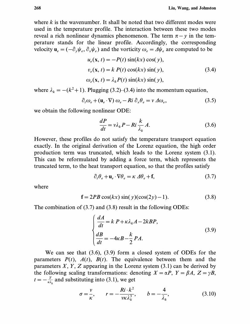
where k is the wavenumber. It shall be noted that two different modes wereused in the temperature profile. The interaction between these two modesreveal a rich nonlinear dynamics phenomenon. The term p−y in the tem-perature stands for the linear profile. Accordingly, the correspondingvelocity ue=(−“yke, “xke) and the vorticity we=Dke are computed to be

ue(x, t)=−P(t) sin(kx) cos(y),

ve(x, t)=k P(t) cos(kx) sin(y),

we(x, t)=lkP(t) sin(kx) sin(y),

(3.4)

where lk=−(k2+1). Plugging (3.2)–(3.4) into the momentum equation,

“twe+(ue ·N) we−Ri “xhe=n Dwe, (3.5)

we obtain the following nonlinear ODE:

dP

dt=nlkP−Ri

k

lkA. (3.6)

However, these profiles do not satisfy the temperature transport equationexactly. In the original derivation of the Lorenz equation, the high orderproduction term was truncated, which leads to the Lorenz system (3.1).This can be reformulated by adding a force term, which represents thetruncated term, to the heat transport equation, so that the profiles satisfy

“the+ue ·Nhe=o Dhe+f, (3.7)

where

f=2PB cos(kx) sin(y)(cos(2y)−1). (3.8)

The combination of (3.7) and (3.8) result in the following ODEs:˛ dAdt=k P+olkA−2kBP,dB

dt=−4oB−

k

2PA.

(3.9)

We can see that (3.6), (3.9) form a closed system of ODEs for theparameters P(t), A(t), B(t). The equivalence between them and theparameters X, Y, Z appearing in the Lorenz system (3.1) can be derived bythe following scaling transformations: denoting X=aP, Y=bA, Z=cB,t=− T

olkand substituting into (3.1), we get

s=n

o, r=−

Ri ·k2

nol3k, b=−

4

lk, (3.10)


and

a=k

olk, b=

Ri·k2

nol3k, c=−

2 Ri k2

nol3k, (3.11)

from which it can be seen that s is the Prandtl number, b is one parameterrelated to the wavenumber, and r is the ratio of the Rayleigh number to thecritical Rayleigh number.

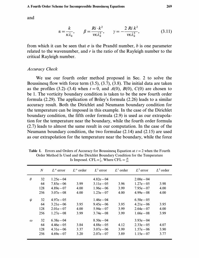
Accuracy Check

We use our fourth order method proposed in Sec. 2 to solve theBoussinesq flow with force term (3.5), (3.7), (3.8). The initial data are takenas the profiles (3.2)–(3.4) when t=0, and A(0), B(0), C(0) are chosen tobe 1. The vorticity boundary condition is taken to be the new fourth orderformula (2.29). The application of Briley’s formula (2.26) leads to a similaraccuracy result. Both the Dirichlet and Neumann boundary condition forthe temperature can be imposed in this example. In the case of the Dirichletboundary condition, the fifth order formula (2.9) is used as our extrapola-tion for the temperature near the boundary, while the fourth order formula(2.7) leads to almost the same result in our computation. In the case of theNeumann boundary condition, the two formulae (2.14) and (2.15) are usedas our extrapolation for the temperature near the boundary, while the force

Table I. Errors and Orders of Accuracy for Boussinesq Equation at t=2 when the FourthOrder Method Is Used and the Dirichlet Boundary Condition for the Temperature

Is Imposed. CFL=12 , Where CFL=Dt

Dx

N L. error L. order L1 error L1 order L2 error L2 order

h 32 1.25e−04 4.82e−04 2.00e−04

64 7.85e−06 3.99 3.11e−05 3.96 1.27e−05 3.98

128 4.89e−07 4.00 1.96e−06 3.99 7.95e−07 4.00

256 3.07e−08 4.00 1.23e−07 4.00 4.99e−08 4.00

k 32 4.97e−05 1.46e−04 6.50e−05

64 3.21e−06 3.95 9.45e−06 3.95 4.21e−06 3.95

128 2.01e−07 4.00 5.94e−07 3.99 2.64e−07 4.00

256 1.27e−08 3.99 3.74e−08 3.99 1.66e−08 3.99

w 32 6.38e−04 8.50e−04 3.93e−04

64 4.46e−05 3.84 4.88e−05 4.12 2.33e−05 4.07

128 4.31e−06 3.37 3.07e−06 3.99 1.57e−06 3.90

256 4.69e−07 3.20 2.07e−07 3.89 1.15e−07 3.77


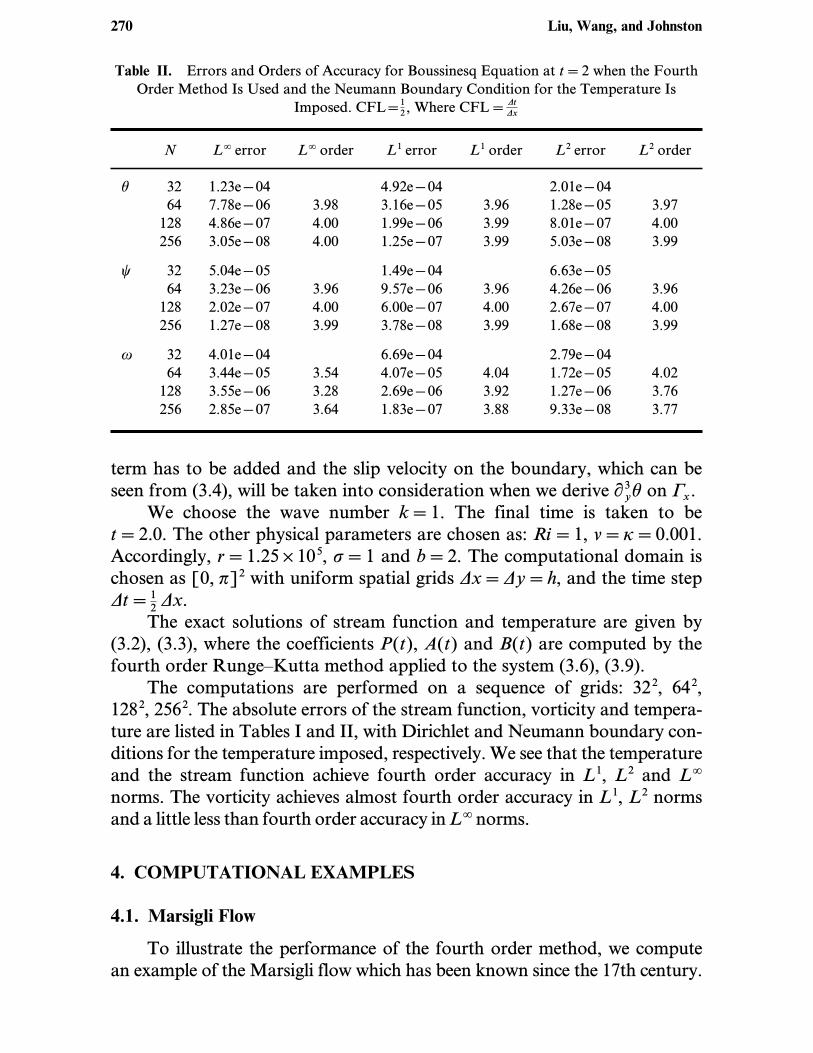
Table II. Errors and Orders of Accuracy for Boussinesq Equation at t=2 when the FourthOrder Method Is Used and the Neumann Boundary Condition for the Temperature Is

Imposed. CFL=12 , Where CFL=Dt

Dx

N L. error L. order L1 error L1 order L2 error L2 order

h 32 1.23e−04 4.92e−04 2.01e−04

64 7.78e−06 3.98 3.16e−05 3.96 1.28e−05 3.97

128 4.86e−07 4.00 1.99e−06 3.99 8.01e−07 4.00

256 3.05e−08 4.00 1.25e−07 3.99 5.03e−08 3.99

k 32 5.04e−05 1.49e−04 6.63e−05

64 3.23e−06 3.96 9.57e−06 3.96 4.26e−06 3.96

128 2.02e−07 4.00 6.00e−07 4.00 2.67e−07 4.00

256 1.27e−08 3.99 3.78e−08 3.99 1.68e−08 3.99

w 32 4.01e−04 6.69e−04 2.79e−04

64 3.44e−05 3.54 4.07e−05 4.04 1.72e−05 4.02

128 3.55e−06 3.28 2.69e−06 3.92 1.27e−06 3.76

256 2.85e−07 3.64 1.83e−07 3.88 9.33e−08 3.77

term has to be added and the slip velocity on the boundary, which can beseen from (3.4), will be taken into consideration when we derive “3yh on Cx.We choose the wave number k=1. The final time is taken to be

t=2.0. The other physical parameters are chosen as: Ri=1, n=o=0.001.Accordingly, r=1.25×105, s=1 and b=2. The computational domain ischosen as [0, p]2 with uniform spatial grids Dx=Dy=h, and the time stepDt=1

2Dx.The exact solutions of stream function and temperature are given by

(3.2), (3.3), where the coefficients P(t), A(t) and B(t) are computed by thefourth order Runge–Kutta method applied to the system (3.6), (3.9).The computations are performed on a sequence of grids: 322, 642,

1282, 2562. The absolute errors of the stream function, vorticity and tempera-ture are listed in Tables I and II, with Dirichlet and Neumann boundary con-ditions for the temperature imposed, respectively. We see that the temperatureand the stream function achieve fourth order accuracy in L1, L2 and L.

norms. The vorticity achieves almost fourth order accuracy in L1, L2 normsand a little less than fourth order accuracy inL. norms.

4. COMPUTATIONAL EXAMPLES

4.1. Marsigli Flow

To illustrate the performance of the fourth order method, we computean example of the Marsigli flow which has been known since the 17th century.


This example can be found in the work of Marsigli (1681). The detailedstory is described in Gill’s book ‘‘Atmosphere-Ocean Dynamics’’ [7]:

It seems that when Marsigli went to Constantinople in 1679 he was told about a

well-known undercurrent in the Bosphorous: ‘‘... for the fisherman of the towns

on the Bosphorous say that the whole stream does not flow in the direction of

Byzantium, but while the upper current which we can see plainly does flow in this

direction, the deep water of the abyss, as it is called, moves in a direction exactly

opposite to that of the upper current and so flows continuously against the current

which is seen.’’ That is, the undercurrent water flows toward the Black Sea from the

Mediterranean. Marsigli reasoned that the effect was due to density differences:

water from the Black Sea is lighter than water from the Mediterranean. The lower

density of the Black Sea can be attributed to lower salinity resulting from river

runoff. He then performed a laboratory experiment: A container is initially divided

in two by a partition. The left side contained water taken from the undercurrent in

the Bosphorous, while the right side contained dyed water having the density of

surface water in the Black Sea. The experiment was to put two holes in the partition

to observe the resulting flow. The flow through the lower hole was in the direction

of the undercurrent in the Bosphorous, while the flow through the upper hole was

in the direction of the surface flow.

We simulated the above physical process in a simple setup: Boussinesqflow with two initially piecewise constant temperatures in an insulated boxW=[0, 8]×[0, 1]. The partition was located at x=4. The temperaturewas chosen to be 1.5 at the left half, which indicated the lower density, 1 atthe right half, which indicated the higher density. (By Boussinesq assump-tion, the density difference can be converted into temperature differencewith the reverse ratio.) The whole flow was at rest at t=0. A no-slipboundary condition was imposed for the velocity and adiabatic boundarycondition was imposed for the temperature. The computational methodwas based on the fourth order scheme discussed above, coupled with fourthorder Runge–Kutta time stepping, as described in Sec. 2.5. Briley’s formula(2.26) was used as the boundary condition for the vorticity. The adiabaticboundary condition imposed for the temperature indicated the use of(2.16), (2.17) to evaluate the temperature at ‘‘ghost’’ points. In our compu-tation, the Reynolds number was chosen to be Re=5000, the Prandtlnumber was chosen to be 1, and the Richardson number Ri, which corre-sponds to the gravity effect, was chosen to be 4. We repeated the computa-tions using two resolutions: 2049×257, 4097×513.Figures 1 and 2 show the computation results on the resolution of

2049×257 of temperature and vorticity at a sequence of times: t1=2,t2=4, t3=6, t4=8, respectively. To save space we only plot thevorticity on the left-half domain [0, 4]×[0, 1]. The vorticity on the right-half domain [4, 8]×[0, 1] is axis-symmetric to that of the left-halfdomain. Once the partition is removed, the flow is driven by the gravityforce. The results indicate clearly the appearance of an upper current


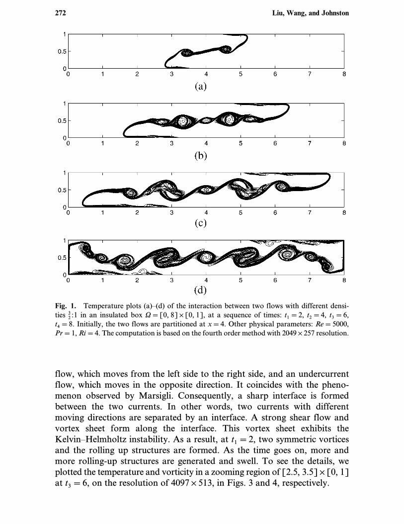
Fig. 1. Temperature plots (a)–(d) of the interaction between two flows with different densi-

ties 32 :1 in an insulated box W=[0, 8]×[0, 1], at a sequence of times: t1=2, t2=4, t3=6,t4=8. Initially, the two flows are partitioned at x=4. Other physical parameters: Re=5000,Pr=1, Ri=4. The computation is based on the fourth order method with 2049×257 resolution.

flow, which moves from the left side to the right side, and an undercurrentflow, which moves in the opposite direction. It coincides with the pheno-menon observed by Marsigli. Consequently, a sharp interface is formedbetween the two currents. In other words, two currents with differentmoving directions are separated by an interface. A strong shear flow andvortex sheet form along the interface. This vortex sheet exhibits theKelvin–Helmholtz instability. As a result, at t1=2, two symmetric vorticesand the rolling up structures are formed. As the time goes on, more andmore rolling-up structures are generated and swell. To see the details, weplotted the temperature and vorticity in a zooming region of [2.5, 3.5]×[0, 1]at t3=6, on the resolution of 4097×513, in Figs. 3 and 4, respectively.


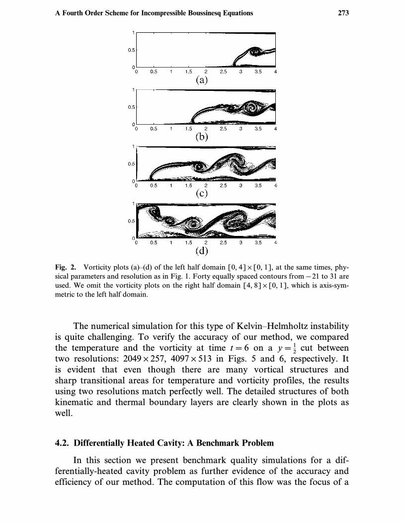
Fig. 2. Vorticity plots (a)–(d) of the left half domain [0, 4]×[0, 1], at the same times, phy-sical parameters and resolution as in Fig. 1. Forty equally spaced contours from −21 to 31 are

used. We omit the vorticity plots on the right half domain [4, 8]×[0, 1], which is axis-sym-metric to the left half domain.

The numerical simulation for this type of Kelvin–Helmholtz instabilityis quite challenging. To verify the accuracy of our method, we comparedthe temperature and the vorticity at time t=6 on a y=1

2cut between

two resolutions: 2049×257, 4097×513 in Figs. 5 and 6, respectively. Itis evident that even though there are many vortical structures andsharp transitional areas for temperature and vorticity profiles, the resultsusing two resolutions match perfectly well. The detailed structures of bothkinematic and thermal boundary layers are clearly shown in the plots aswell.

4.2. Differentially Heated Cavity: A Benchmark Problem

In this section we present benchmark quality simulations for a dif-ferentially-heated cavity problem as further evidence of the accuracy andefficiency of our method. The computation of this flow was the focus of a


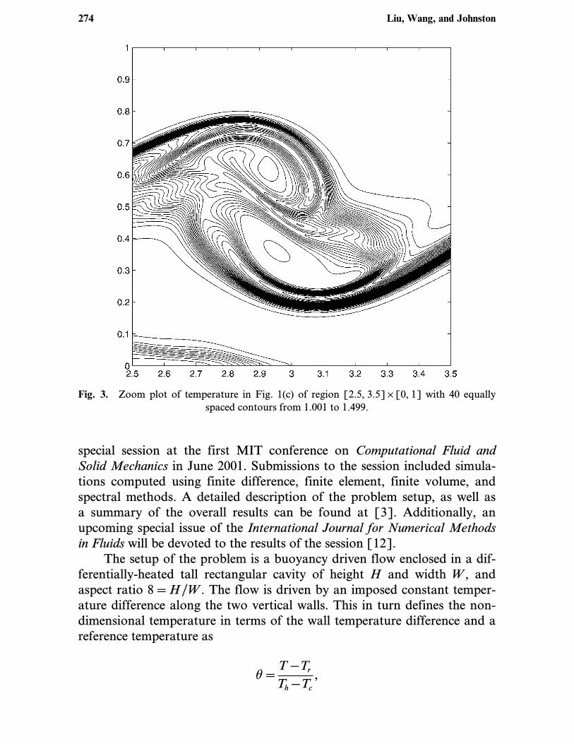
Fig. 3. Zoom plot of temperature in Fig. 1(c) of region [2.5, 3.5]×[0, 1] with 40 equallyspaced contours from 1.001 to 1.499.

special session at the first MIT conference on Computational Fluid andSolid Mechanics in June 2001. Submissions to the session included simula-tions computed using finite difference, finite element, finite volume, andspectral methods. A detailed description of the problem setup, as well asa summary of the overall results can be found at [3]. Additionally, anupcoming special issue of the International Journal for Numerical Methodsin Fluids will be devoted to the results of the session [12].The setup of the problem is a buoyancy driven flow enclosed in a dif-

ferentially-heated tall rectangular cavity of height H and width W, andaspect ratio 8=H/W. The flow is driven by an imposed constant temper-ature difference along the two vertical walls. This in turn defines the non-dimensional temperature in terms of the wall temperature difference and areference temperature as

h=T−TrTh−Tc

,


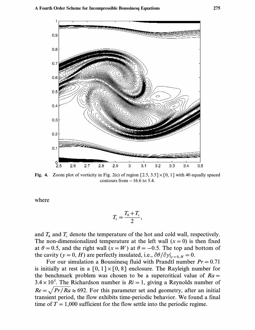
Fig. 4. Zoom plot of vorticity in Fig. 2(c) of region [2.5, 3.5]×[0, 1] with 40 equally spacedcontours from −16.6 to 5.4.

where

Tr=Th+Tc2,

and Th and Tc denote the temperature of the hot and cold wall, respectively.The non-dimensionalized temperature at the left wall (x=0) is then fixedat h=0.5, and the right wall (x=W) at h=−0.5. The top and bottom ofthe cavity (y=0, H) are perfectly insulated, i.e., “h/“y|y=0, H=0.For our simulation a Boussinesq fluid with Prandtl number Pr=0.71

is initially at rest in a [0, 1]×[0, 8] enclosure. The Rayleigh number forthe benchmark problem was chosen to be a supercritical value of Ra=3.4×105. The Richardson number is Ri=1, giving a Reynolds number of

Re=`Pr/Ra % 692. For this parameter set and geometry, after an initialtransient period, the flow exhibits time-periodic behavior. We found a finaltime of T=1,000 sufficient for the flow settle into the periodic regime.


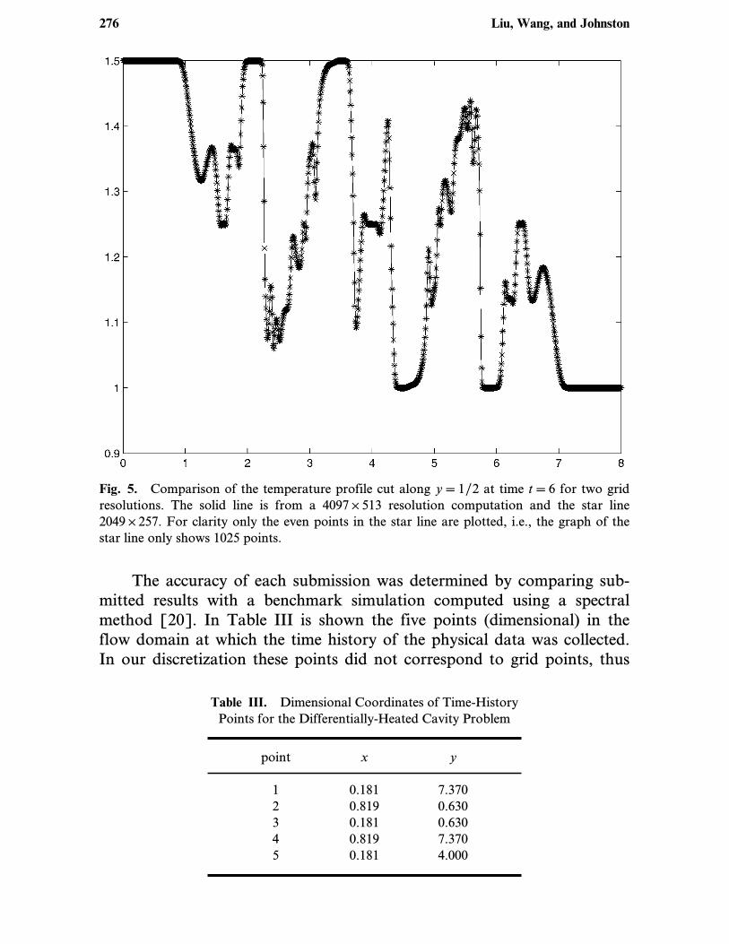
Fig. 5. Comparison of the temperature profile cut along y=1/2 at time t=6 for two gridresolutions. The solid line is from a 4097×513 resolution computation and the star line2049×257. For clarity only the even points in the star line are plotted, i.e., the graph of thestar line only shows 1025 points.

The accuracy of each submission was determined by comparing sub-mitted results with a benchmark simulation computed using a spectralmethod [20]. In Table III is shown the five points (dimensional) in theflow domain at which the time history of the physical data was collected.In our discretization these points did not correspond to grid points, thus

Table III. Dimensional Coordinates of Time-History

Points for the Differentially-Heated Cavity Problem

point x y

1 0.181 7.370

2 0.819 0.630

3 0.181 0.630

4 0.819 7.370

5 0.181 4.000


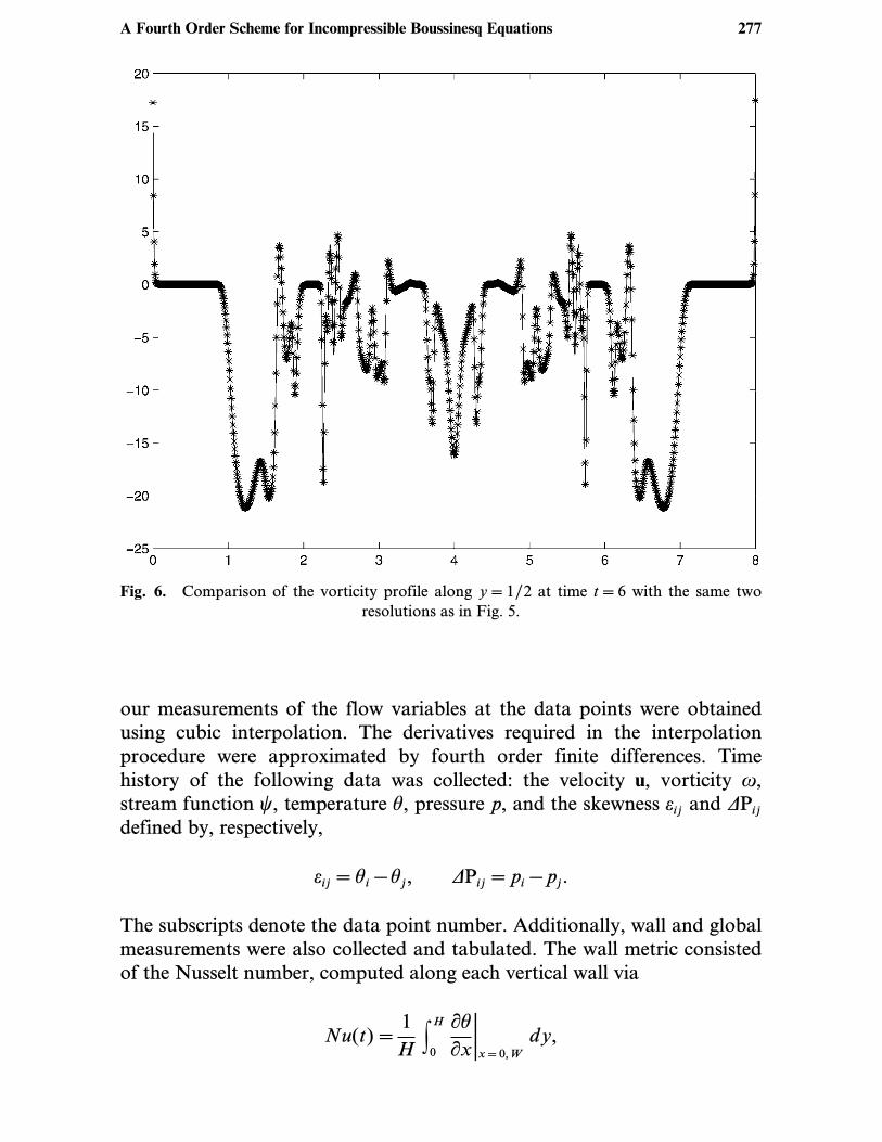
Fig. 6. Comparison of the vorticity profile along y=1/2 at time t=6 with the same tworesolutions as in Fig. 5.

our measurements of the flow variables at the data points were obtainedusing cubic interpolation. The derivatives required in the interpolationprocedure were approximated by fourth order finite differences. Timehistory of the following data was collected: the velocity u, vorticity w,stream function k, temperature h, pressure p, and the skewness eij and DPijdefined by, respectively,

eij=hi−hj, DPij=pi−pj.

The subscripts denote the data point number. Additionally, wall and globalmeasurements were also collected and tabulated. The wall metric consistedof the Nusselt number, computed along each vertical wall via

Nu(t)=1

HFH0

“h“x:x=0, W

dy,


where H=8 and W=1. Finally, two global metrics were collected in theform of the square-root of the kinetic energy and the entropy,

u1(t)== 12A

FA

u ·u dA, w(t)== 12A

FA

w2 dA,

where A=8, the area of the enclosure.The period of each measurement was computed by finding the zero

crossings of mean adjusted data taken over 10 periods starting at approx-imately T=950. Simpson’s rule was used to approximate all integrals, andthe derivative in the evaluation of Nu was approximated to fourth ordervia finite differences. The stencil, e.g., along x=0, included the points{hi, j: i=−1,..., 4} with the h−1, j ghost point defined as discussed inSec. 2.2.1.Our numerical scheme is based on the (w, k) formulation, thus for the

pressure measurements we solve the derived pressure Poisson equation

gp=(N ·u)2−(Nu) : (Nu)T+Ri hy, (4.1)

using a second order finite difference scheme for non-staggered grids basedon local pressure boundary conditions. The scheme was proposed in [13],and here we briefly explain the key aspect of the method. Note that (4.1)follows by taking the divergence of the momentum equation in (1.1) andusing N ·u=0 to simplify the result. One can then view (4.1) as a replace-ment for the incompressibility condition, but with the additional require-ment that

N ·u|C=0. (4.2)

A natural boundary condition for (4.1) is

“p“n=(ng u+Ri [h) ·n, (4.3)

a Neumann boundary condition derived by dotting the momentum equa-tion in (1.1) with the unit normal n at the boundary. Here [ is the unitvector in the y direction. The difficulty numerically in applying (4.3) is thatit requires an approximation of the Laplacian at the boundary. Specifically,the stencil of the second order centered approximation of g alongthe boundary C requires an undefined ‘‘ghost point’’ lying outside of thecomputational domain. We remedy the situation as follows: Consider the


horizontal boundary segment Cx along y=0. A second order centeredapproximation of (ng u) ·n at the (i, 0) grid point is given by

(ng u) ·n=n(vxx+vyy)

=n(vi+1, 0+vi−1, 0+vi, 1+vi, −1−4vi, 0)/h2+O(h2)

=n(vi, 1+vi, −1)/h2+O(h2), (4.4)

where we have used u|C=0, which requires the value vi, −1. Discretizing theboundary condition N ·u=0 in (4.2) as

0=N ·u=ux+vy=0+vy=(vi, 1−vi, −1)

2h+O(h2),

where again we have used u|C=0, giving vi, −1=vi, 1+O(h3), implying in

(4.4) that one should take vi, −1=vi, 1. The result is the following approxi-mation for the Neumann boundary condition (4.3):

“p“y:(xi, 0)

=2n

h2vi, 1+Ri hi, 0.

We note the similarly in philosophy between the derivation of local pres-sure boundary conditions and local vorticity boundary conditions. Withthe discrete Neumann boundary condition a second order centered discre-tization of (4.1) is efficiently solved using FFT methods, resulting in a glo-bally second order accurate solution; see [13].Two grid resolutions (Nx+1)×(Ny+1), equally-spaced in each coor-

dinate direction, were computed: 97×769, and 129×1025. In each caseDx=Dy. The simulations were run until a final non-dimensional time ofT=1000. A fixed Dt was used for each simulation as determined by (2.37)with CFL=0.75 and ||u||.=1.0. The CFL number was chosen to be lessthan 1 in order to avoid instability due to the time step during the initialtransient where the velocity exceeds ||u||.=1.0.In Tables IV and V are shown tabulated results at the two grid resolu-

tions. Point metrics without subscripts are for the data point 1, (x, y)=(0.181, 7.370). This data was used for comparison of submissions to thespecial session. Overall the results at the two resolutions are in goodagreement. The largest discrepancies are seen in the DP pressure measure-ments. This is attributable to the fact that the pressure is only recovered tosecond order accuracy. However, we emphasize that the pressure compu-tation does not affect the overall accuracy of the numerical scheme since itis performed only to collect the pressure point data.


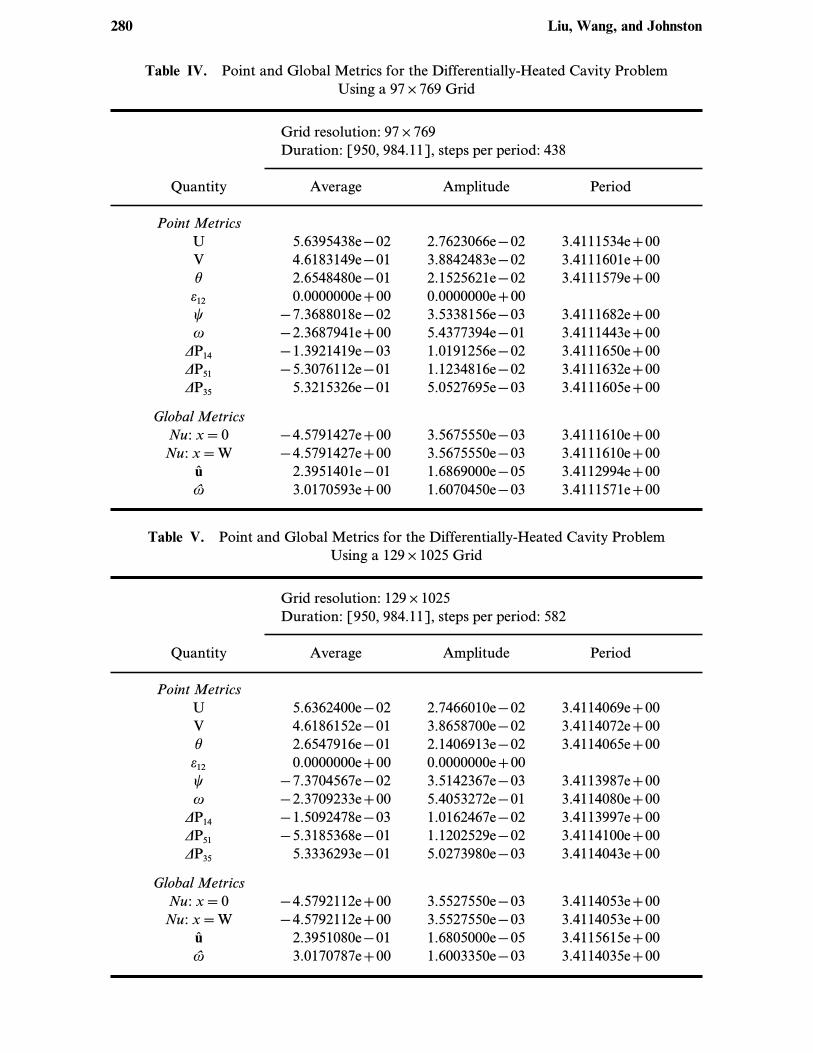
Table IV. Point and Global Metrics for the Differentially-Heated Cavity Problem

Using a 97×769 Grid

Grid resolution: 97×769Duration: [950, 984.11], steps per period: 438

Quantity Average Amplitude Period

Point Metrics

U 5.6395438e−02 2.7623066e−02 3.4111534e+00

V 4.6183149e−01 3.8842483e−02 3.4111601e+00

h 2.6548480e−01 2.1525621e−02 3.4111579e+00

e12 0.0000000e+00 0.0000000e+00

k −7.3688018e−02 3.5338156e−03 3.4111682e+00

w −2.3687941e+00 5.4377394e−01 3.4111443e+00

DP14 −1.3921419e−03 1.0191256e−02 3.4111650e+00

DP51 −5.3076112e−01 1.1234816e−02 3.4111632e+00

DP35 5.3215326e−01 5.0527695e−03 3.4111605e+00

Global Metrics

Nu: x=0 −4.5791427e+00 3.5675550e−03 3.4111610e+00

Nu: x=W −4.5791427e+00 3.5675550e−03 3.4111610e+00

u 2.3951401e−01 1.6869000e−05 3.4112994e+00

w 3.0170593e+00 1.6070450e−03 3.4111571e+00

Table V. Point and Global Metrics for the Differentially-Heated Cavity Problem

Using a 129×1025 Grid

Grid resolution: 129×1025Duration: [950, 984.11], steps per period: 582

Quantity Average Amplitude Period

Point Metrics

U 5.6362400e−02 2.7466010e−02 3.4114069e+00

V 4.6186152e−01 3.8658700e−02 3.4114072e+00

h 2.6547916e−01 2.1406913e−02 3.4114065e+00

e12 0.0000000e+00 0.0000000e+00

k −7.3704567e−02 3.5142367e−03 3.4113987e+00

w −2.3709233e+00 5.4053272e−01 3.4114080e+00

DP14 −1.5092478e−03 1.0162467e−02 3.4113997e+00

DP51 −5.3185368e−01 1.1202529e−02 3.4114100e+00

DP35 5.3336293e−01 5.0273980e−03 3.4114043e+00

Global Metrics

Nu: x=0 −4.5792112e+00 3.5527550e−03 3.4114053e+00

Nu: x=W −4.5792112e+00 3.5527550e−03 3.4114053e+00

u 2.3951080e−01 1.6805000e−05 3.4115615e+00

w 3.0170787e+00 1.6003350e−03 3.4114035e+00


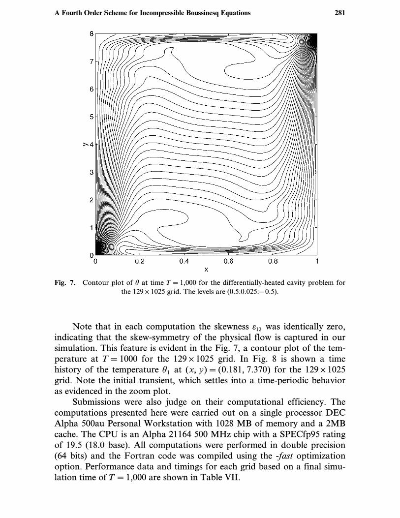
Fig. 7. Contour plot of h at time T=1,000 for the differentially-heated cavity problem forthe 129×1025 grid. The levels are (0.5:0.025:−0.5).

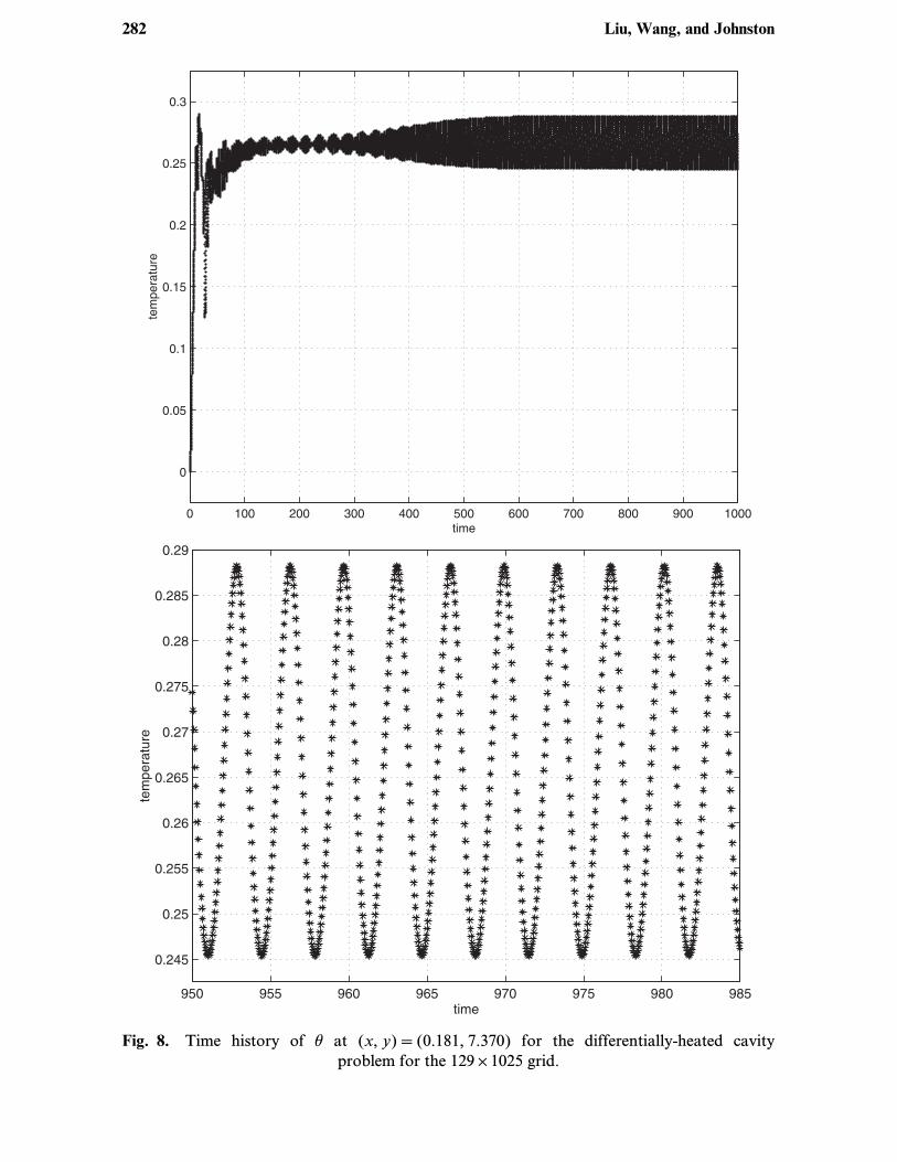
Note that in each computation the skewness e12 was identically zero,indicating that the skew-symmetry of the physical flow is captured in oursimulation. This feature is evident in the Fig. 7, a contour plot of the tem-perature at T=1000 for the 129×1025 grid. In Fig. 8 is shown a timehistory of the temperature h1 at (x, y)=(0.181, 7.370) for the 129×1025grid. Note the initial transient, which settles into a time-periodic behavioras evidenced in the zoom plot.Submissions were also judge on their computational efficiency. The

computations presented here were carried out on a single processor DECAlpha 500au Personal Workstation with 1028 MB of memory and a 2MBcache. The CPU is an Alpha 21164 500 MHz chip with a SPECfp95 ratingof 19.5 (18.0 base). All computations were performed in double precision(64 bits) and the Fortran code was compiled using the -fast optimizationoption. Performance data and timings for each grid based on a final simu-lation time of T=1,000 are shown in Table VII.


0 100 200 300 400 500 600 700 800 900 1000

0

0.05

0.1

0.15

0.2

0.25

0.3

time

tem

pe

ratu

re

950 955 960 965 970 975 980 985

0.245

0.25

0.255

0.26

0.265

0.27

0.275

0.28

0.285

0.29

time

tem

pera

ture

Fig. 8. Time history of h at (x, y)=(0.181, 7.370) for the differentially-heated cavityproblem for the 129×1025 grid.


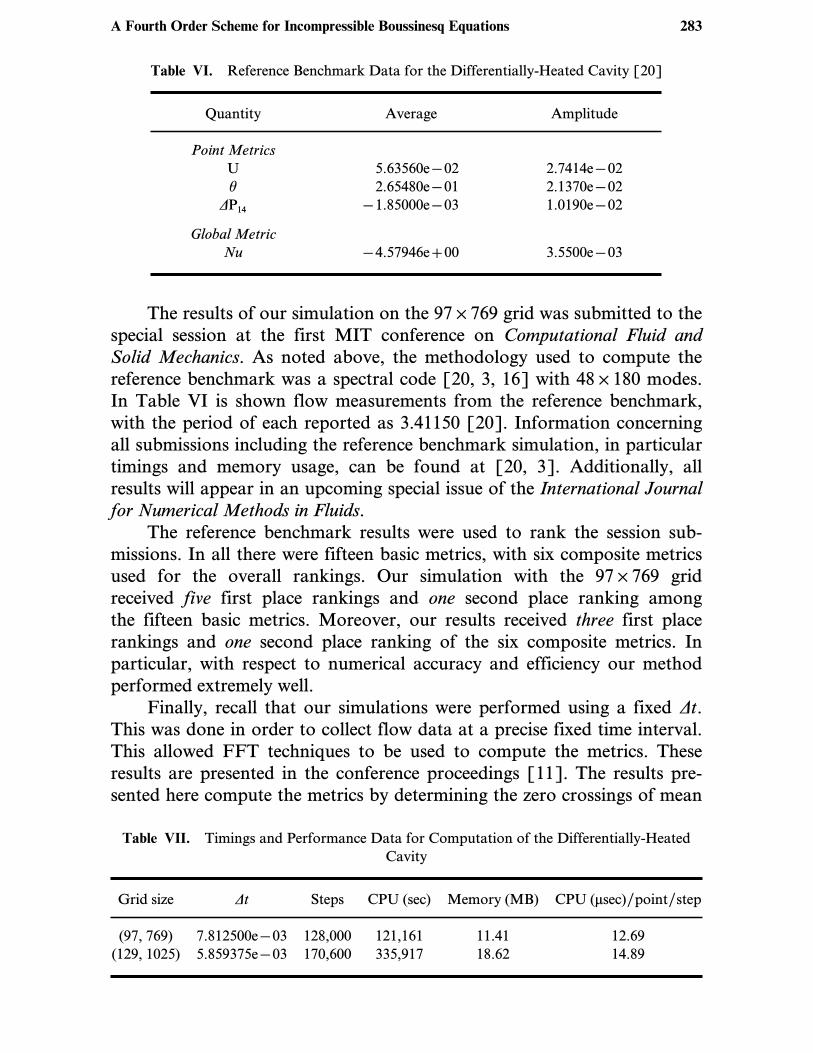
Table VI. Reference Benchmark Data for the Differentially-Heated Cavity [20]

Quantity Average Amplitude

Point Metrics

U 5.63560e−02 2.7414e−02

h 2.65480e−01 2.1370e−02

DP14 −1.85000e−03 1.0190e−02

Global Metric

Nu −4.57946e+00 3.5500e−03

The results of our simulation on the 97×769 grid was submitted to thespecial session at the first MIT conference on Computational Fluid andSolid Mechanics. As noted above, the methodology used to compute thereference benchmark was a spectral code [20, 3, 16] with 48×180 modes.In Table VI is shown flow measurements from the reference benchmark,with the period of each reported as 3.41150 [20]. Information concerningall submissions including the reference benchmark simulation, in particulartimings and memory usage, can be found at [20, 3]. Additionally, allresults will appear in an upcoming special issue of the International Journalfor Numerical Methods in Fluids.The reference benchmark results were used to rank the session sub-

missions. In all there were fifteen basic metrics, with six composite metricsused for the overall rankings. Our simulation with the 97×769 gridreceived five first place rankings and one second place ranking amongthe fifteen basic metrics. Moreover, our results received three first placerankings and one second place ranking of the six composite metrics. Inparticular, with respect to numerical accuracy and efficiency our methodperformed extremely well.Finally, recall that our simulations were performed using a fixed Dt.

This was done in order to collect flow data at a precise fixed time interval.This allowed FFT techniques to be used to compute the metrics. Theseresults are presented in the conference proceedings [11]. The results pre-sented here compute the metrics by determining the zero crossings of mean

Table VII. Timings and Performance Data for Computation of the Differentially-Heated

Cavity

Grid size Dt Steps CPU (sec) Memory (MB) CPU (msec)/point/step

(97, 769) 7.812500e−03 128,000 121,161 11.41 12.69

(129, 1025) 5.859375e−03 170,600 335,917 18.62 14.89


adjusted data as describe above, which we found to be more accurate.Thus, a fixed Dt is not necessary and in fact adds significantly to the totalcomputational time. This was determined by performing a simulation andallowing for a variable time step with the 97×769 grid and CFL=1.0.Allowing for a variable time step by monitoring ||u||. during the run todetermine Dt resulted in a one-third reduction in the total runtime.

ACKNOWLEDGMENTS

The work of J.-G. Liu was supported by NSF Grant DMS-0107218.

REFERENCES

1. Bell, J. B., and Marcus, D. L. (1992). A Second-order projection method for variable-

density flows. J. Comput. Phys. 101, 334–348.

2. Briley, W. R. (1971). A numerical study of laminar separation bubbles using the

Navier–Stokes equations. J. Fluid Mech. 47, 713–736.

3. Christon, M. (2001). Results Summary: Special session on computational predictability of

natural convection flows in enclosures, http://wotan.me.unm.edu/’christon/mit_convec-

tion/summary/

4. E, Weinan, and Liu, J.-G. (1996). Vorticity boundary condition for finite difference

schemes. J. Comput. Phys. 124, 368–382.

5. E, Weinan, and Liu, J.-G. (1996). Essentially compact schemes for unsteady viscous

incompressible flows. J. Comput. Phys. 126, 122–138.

6. E, Weinan, and Shu, Chi-Wang (1994). Small-scale structures in Boussinesq convection.

Phys. Fluids 6 (1), 49–58.

7. Gill, A. E. (1982). Atmosphere-Ocean Dynamics, Academic Press.

8. Glowinski, R., and Pironneau, O. (1979). Numerical methods for the first biharmonic

equation and for the two-dimensional Stokes problem. SIAM Rev. 21, 167–212.

9. Henshaw, W. D., Kreiss, H. O., and Reyna, L. G. M. (1994). A fourth-order accurate

difference approximation for the incompressible Navier–Stokes equations. Comput. and

Fluids 23, 575–593.

10. Hou, T. Y., and Wetton, B., Stable fourth order stream-function methods for incom-

pressible flows with boundaries, unpublished.

11. Johnston, H., and Krasny, R. (2001). Computational predictability of natural convection

flows in enclosures: A benchmark problem. In Bathe, K. J. (ed.), Computational Fluids and

Solid Mechanics (Conference Proceedings), Elsevier Science.

12. Johnston, H., and Krasny, R. (2002). Fourth order finite difference simulation of a dif-

ferentially-heated cavity. To appear in Int. J. Num. Meth. Fluids.

13. Johnston, H., and Liu J.-G. (2002). Finite difference schemes for incompressible flow

based on local pressure boundary conditions. J. Comput. Phys. 180, 120–154.

14. Orszag, S. A., and Israeli, M. (1974). Numerical simulation of viscous incompressible

flows. Ann. Rev. Fluid Mech. 6, 281–318.

15. Quartapelle, L. (1983). Numerical Solution of the Incompressible Navier–Stokes Equations,

Birkhauser, Berlin.

16. Quéré, P. L., and Behnia, M. (1998). From onset of unsteadiness to chaos in a differen-

tially heated cavity. J. Fluid Mech. 359, 81–107.


17. Thom, A. (1933). The flow past circular cylinders at low speeds, Proc. Roy. Soc. A 141,

651–669.

18. Thorpe, S. A. (1968). On standing internal gravity waves of finite amplitude. J. Fluid

Mech. 32, 489–528.

19. Thorpe, S. A. (1969). Experiments on the instability of stratified shear flows: Immiscible

fluids. J. Fluid Mech. 39, 25–48.

20. Xin, S., and Le Quéré, P. L. (2001). In Bathe, K. J. (ed.), Computational Fluids and Solid

Mechanics (Conference Proceedings), Elsevier Science.

21. Wang, C., and Liu, J.-G. (2002). Analysis of finite difference schemes for unsteady

Navier–Stokes equations in vorticity formulation. Numer. Math. 91, 543–576.

22. Wang, C., and Liu, J.-G., Fourth order convergence of compact finite difference solvers

for 2D incompressible flow. Accepted for publication in Comm. in Appl. Anal.

23. Wang, C., Liu, J.-G., and Johnston, H. Analysis of a fourth order finite difference method

for incompressible Boussinesq equations. Submitted to Numer. Math.


Documents

A Fourth Order Scheme for Incompressible Boussinesq …cwang/LWJ03.pdf · A Fourth Order Scheme for Incompressible ... allows the solution of the temperature equation to fourth order