A FRAMEWORK FOR INVERTIBLE, REAL-TIME ... FRAMEWORK FOR INVERTIBLE, REAL-TIME CONSTANT-Q TRANSFORMS NICKI HOLIGHAUS, MONIKA DORFLER, GINO ANGELO VELASCO,¨ AND THOMAS GRILL Abstract

A FRAMEWORK FOR INVERTIBLE, REAL-TIME CONSTANT-Q

TRANSFORMS

NICKI HOLIGHAUS, MONIKA DORFLER, GINO ANGELO VELASCO,AND THOMAS GRILL

Abstract. Audio signal processing frequently requires time-frequency repre-sentations and in many applications, a non-linear spacing of frequency-bandsis preferable. This paper introduces a framework for efficient implementa-tion of invertible signal transforms allowing for non-uniform and in particularnon-linear frequency resolution. Non-uniformity in frequency is realized by ap-plying nonstationary Gabor frames with adaptivity in the frequency domain.The realization of a perfectly invertible constant-Q transform is described indetail. To achieve real-time processing, independent of signal length, slice-wise processing of the full input signal is proposed and referred to as sliCQtransform.

By applying frame theory and FFT-based processing, the presented ap-proach overcomes computational inefficiency and lack of invertibility of clas-sical constant-Q transform implementations. Numerical simulations evaluatethe efficiency of the proposed algorithm and the method’s applicability is il-lustrated by experiments on real-life audio signals.

1. Introduction

Analysis, synthesis and processing of sound is commonly based on the repre-sentation of audio signals by means of time-frequency dictionaries. The short-timeFourier transform (STFT), also referred to as Gabor transform, is a widely used tooldue to its straight-forward interpretation and FFT-based implementation, which en-sure efficiency and invertibility [15, 7]. STFT features a uniform time and frequencyresolution and a linear spacing of the time frequency bins.

In contrast, the constant-Q transform (CQT), originally introduced in [22] and inmusic processing by J. Brown [2], provides a frequency resolution that depends ongeometrically spaced center frequencies of the analysis windows. In particular, theQ-factor, i.e. the ratio of center frequency to bandwidth of each window, is constantover all frequency bins; the constant Q-factor leads to a finer frequency resolutionin low frequencies whereas time resolution improves with increasing frequency. Thisprinciple makes the constant-Q transform well-suited for audio data, since it betterreflects the resolution of the human auditory system than the linear frequency-spacing provided by the FFT, cf. [20] and references therein. Furthermore, musicalcharacteristics such as overtone structures remain invariant under frequency shiftsin a constant-Q transform, which is a natural feature from a perception point ofview. In speech and music processing, perception-based considerations are impor-tant, which is one of the reasons why CQTs, due to their previously discussed

Date: September 27, 2012.

1

2 N. HOLIGHAUS, M. DORFLER, G. VELASCO, AND T. GRILL

properties, are often desirable in these fields. An example of a CQ-transform, ob-tained with our algorithm, is shown in Figure 1.

The principal idea of CQT is reminiscent of wavelet transforms, compare [19].As opposed to wavelet transforms, the original CQT is not invertible and does notrely on any concept of (orthonormal) bases. On the other hand, the number ofbins (frequency channels) per octave is much higher in the CQT than most tra-ditional wavelet techniques would allow for. Partly due to this requirement, thecomputational efficiency of the original transform as well as its improved versions,cf. [3], may often be insufficient. Moreover, the lack of invertibility of existing CQTshas become an important issue: for some desired applications, such as extractionand modification, e.g. transposition, of distinct parts of the signal, the unbiasedreconstruction from analysis coefficients is crucial. Approximate methods for recon-struction from constant-Q coefficients have been proposed before, in particular forsignals which are sparse in the frequency domain [5] and by octave-wise processingin [18].

In the present contribution, we are interested in inversion in the sense of perfectreconstruction, i.e. up to numerical precision; to this end, we investigate a new ap-proach to constant-Q signal processing. The presented framework has the followingcore properties:

(1) Relying on concepts from frame theory, [15], we suggest the implementa-tion of a constant-Q transform using the nonstationary Gabor transform(NSGT), which guarantees perfect invertibility. This perfectly invertibleconstant-Q transform is subsequently called constant-Q nonstationary Ga-bor transform (CQ-NSGT).

(2) We introduce a preprocessing step by slicing the signal to pieces of (usuallyuniform) finite length. Together with FFT-based methods, this allows forbounded delay and results in linear processing time. Thus, our algorithmlends itself to real-time processing and the resulting transform is referredto as sliced constant-Q transform (sliCQ).

NSGTs, introduced in [11, 1], generalize the classical sampled short-time Fouriertransform or Gabor transform [15, 10]. They allow for fast, FFT-based implemen-tation of both analysis and reconstruction under mild conditions on the analysiswindows. The CQ-NSGT was first presented in [21]; the frequency-resolution ofthe proposed CQ-NSGT is essentially identical to that of the CQT, cf. Figure 1 foran example.

The main drawback of the CQ-NSGT is the inherent necessity to obtain a Fouriertransform of the entire signal prior to actual processing. This problem prohibitsreal-time implementation and is overcome by a slicing step, which preserves theperfect reconstruction property. However, blocking effects and time-aliasing maybe observed if the coefficients are modified in applications such as de-noising ortransposition and time-shift of certain signal components. While slicing the signalnaturally introduces a trade-off between delay and finest possible frequency resolu-tion, the parameters can be chosen to suppress blocking artifacts and to leave theconstant-Q coefficient structure intact.

The rest of this paper is organized as follows. In Section 2 we introduce theconcepts of frames as overcomplete, stable spanning sets, with a focus on nonsta-tionary Gabor (NSG) systems and their properties. We recall the conditions forthese systems to constitute so-called painless frames, a special case that allows for

A FRAMEWORK FOR INVERTIBLE, REAL-TIME CONSTANT-Q TRANSFORMS 3

time (seconds)

freq

uenc

y (H

z)

Kafziel − dB−scaled Regular Gabor Transform Spectrogram

0 2 4 6 8 10 12 50

200

800

3200

1280022050

time (seconds)

freq

uenc

y (H

z)

Kafziel − dB−scaled CQ−NSGT Spectrogram

0 2 4 6 8 10 12 50

200

800

3200

1280022050

Figure 1. Time-frequency representations on a logarithmicallyscaled frequency axis: STFT spectrogram (top) and constant-QNSGT spectrogram (bottom).

straightforward inversion. Section 3 describes the construction of the CQ-NSGT byNSG frames with adaptivity in the frequency domain. This is the starting point forthe sliCQ transform, which is explored in Section 4. After giving the general idea,we describe interpretation of the sliCQ-coefficients in relation to the full-lengthtransform in Section 4.3. Subsequently, Section 5 is concerned with an analysis ofthe transforms’ numerical properties, in particular computation time and complex-ity, as well as the quality of approximation of the CQ-NSGT coefficients by thesliCQ, accompanied by a set of simulations. Finally, in Section 6 the CQ-NSGT isapplied and evaluated in the analysis and processing of real-life signals. The paperis closed by a short summary and conclusion.

2. Nonstationary Gabor Frames

Frames, first mentioned in [8], also cf. [4, 15], generalize (orthonormal) bases andallow for redundancy and thus design flexibility in signal representations. Framesmay be tailored to a specific application or certain requirements such as a constant-Q frequency resolution. Loosely speaking, we wish to represent a given signal ofinterest as a sum of the frame members ϕn,k, weighted by coefficients cn,k:

(1) f

¸

n,k

cn,kϕn,k.


The double indexes pn, kq allude to the fact that each atom has a certain locationand concentration in time and frequency. Frame theory establishes conditions underwhich an expansion of the form (1) can be obtained with coefficients leading tostable, perfect reconstruction.

For this contribution, we only consider frames for CL, that is vector spaces of

finite, discrete signals, understood as functions f, g on CL. We denote by xf, gy the

inner product of f and g, i.e. xf, gy °L1

l0 f rlsgrls and f2 a

xf, fy. The struc-tures introduced here can easily be extended to the Hilbert space of quadraticallyintegrable functions, L2

pRq.

2.1. Frames. Consider a collection of atoms ϕn,k P CL with pn, kq P IN IK forfinite index sets IN , IK . We then define the frame operator S by

(2) Sf ¸

n,k

xf, ϕn,kyϕn,k,

for all f P CL. If the linear operator S is invertible on CL, then the set of functionstϕn,ku

pn,kqPINIK , is a frame1. In this case, we may define a dual frame by

(3) ϕn,k S1ϕn,k

and reconstruction from the coefficients cn,k xf, ϕn,ky is straight-forward:

f S1Sf

¸

n,k

xf, ϕn,kyS1ϕn,k

¸

n,k

cn,kϕn,k

SS1f

¸

n,k

xf,S1ϕn,kyϕn,k

¸

n,k

xf, ϕn,kyϕn,k.

We next introduce a case of particular importance, the so-called Gabor frames,for which the elements ϕn,k are obtained from a single window ϕ by time- andfrequency-shifts along a lattice. Let Tx and Mω denote a time-shift by x and afrequency shift (or modulation) by ω, i.e.

Txf rls f rl xs and Mωf rls e2πilωLf rls,

where l x is considered modulo L. Furthermore, we use the normalization

Ff rjs f rjs 1?

L

L1

l0

f rlse2πiljL

for the discrete Fourier transform of f . It follows that FpTxfq Mxf and

FpMωfq Tω f .Fixing a time-shift parameter a and a frequency-shift parameter b, with La, Lb P

N, we call the collection of atoms G tϕn,k MkbTnaϕupn,kqPINIK , with IN

IK ZLa ZLb, a Gabor system. If G is a frame, it is called a Gabor frame. ForGabor frames, the frame coefficients are given by samples of the short-time Fouriertransform (STFT) of f with respect to the window ϕ:

cn,k xf, ϕn,ky xf,MkbTnaϕy

L1

l0

f rlsϕrl nase2πilkbL.(4)

1Note that, if tϕn,k , pn, kq P IN IKu is an orthonormal basis, then S is the identity operator.


In a general setting, the inversion of the operator S poses a problem in numericalrealization of frame analysis. However, for Gabor frames, it was shown in [6], thatunder certain conditions, usually fulfilled in practical applications, S is diagonal,and a dual frame can be calculated easily. This situation of painless non-orthogonalexpansions can now be generalized to allow for adaptive resolution.

2.2. Frequency-Adaptive Painless Nonstationary Gabor Frames. In clas-sical Gabor frames, we obtain all samples of the STFT in (4) by applying the samewindow ϕ, shifted along a regular set of sampling points and taking an FFT ofthe same length. In order to achieve adaptivity of the resolution in either time orfrequency, we relax the regularity of classical Gabor frames to derive nonstationaryGabor frames.

The original motivation for the introduction of NSGT was the desire to adaptboth window size and sampling density in time, cf. [11, 1], in order to accuratelyresolve transient signal components. Here, we apply the same idea in frequency, i.e.adapt both the bandwidth and sampling density in frequency. From an algorithmicpoint of view, we apply a nonstationary Gabor system to the Fourier transform ofthe input signal.

The windows are constructed directly in the frequency domain by taking real-valued filters gk centered at ωk. The inverse Fourier transforms qgk : F1gkare the time-reverse impulse responses of the corresponding (frequency-adaptive)filters. Therefore, we let qgk, k P IK , denote the members of a finite collection ofband-limited windows, well-localized in time, whose Fourier transforms gk F qgkare centered around possibly irregularly (or, e.g. geometrically) spaced frequencypoints ωk.

Then, we select frequency dependent time-shift parameters (hop-sizes) ak asfollows: if the support (the interval where the vector is nonzero) of gk is containedin an interval of length Lk, then ak is chosen such that

(5) ak ¤L

Lk

for all k.

In other words, the time-sampling points have to be chosen dense enough to guar-antee (5). If we denote by gn,k the modulation of gk by nak, i.e. gn,k M

nakgk,

then we obtain the frame members ϕn,k by setting

ϕn,k gn,k F1pM

nakgkq Tnak

qgk,

where k P IK and n 0, . . . , Lak1. The system Gpg, aq : tgn,k Tnakgkun,k is

a painless nonstationary Gabor system, as described in [1], for CL. We also defineg : tgk P CL

ukPIK and a : takukPIK . By Parseval’s formula, we see that theframe coefficients can be written as

(6) cn,k xf,gn,ky xf ,Mnak

gky.

For convenience, we use the notation c : tckukPIK : ttcn,kuLak1n0 ukPIK to refer

to the full set of coefficients and channel coefficients, respectively. By abuse ofnotation, we indicate by c P CLak|IK | that c is an irregular array with |IK |

columns, the k-th column possessing Lak entries. The NSG coefficients can becomputed using the following algorithm.

Here (I)FFTN denotes a (inverse) Fast Fourier transform of length N , includ-ing the necessary periodization or zero-padding preprocessing to convert the inputvector to the correct length N . The analysis algorithm above is complemented by


Algorithm 1 NSG analysis: c CQ-NSGTLpf,g, aq

1: Initialize f, gk for all k P IK2: f FFTLpfq

3: for k P IK , n 0, . . . , Lak 1 do

4: ck a

Lak IFFTLakpfgkq

5: end for

Algorithm 2, an equally simple synthesis algorithm that synthesizes a signal f froma set of coefficients c.

Algorithm 2 NSG synthesis: f iCQ-NSGTLpc, g, aq

1: Initialize cn,k, rgk for all n 0, . . . , Lak 1, k P IK2: for k P Ik do3: fk

a

akL FFTLakpckq

4: end for5: f

°

kPIKfk rgk

6: f IFFTLpfq

If Gpg, aq and Gpg, aq are a pair of dual frames, then we can reconstruct a functionperfectly from its NSG analysis coefficients. For more details and a proof of thefollowing propositions, see Appendix 8.1.

Proposition 1. Let Gpg, aq tgn,k Tnakgkun,k and Gpg, aq tgn,k Tnak

rgkun,kbe a pair of dual frames. If c is the output of CQ-NSGTLpf,g, aq (Algorithm 1),

then the output f of iCQ-NSGTLpc, g, aq (Algorithm 2) equals f , i.e.

(7) f f, for all f P CL.

The remaining problem is to ascertain that Gpg, aq is a frame and to compute thedual frame. The following proposition is a discrete version of an equivalent resultfor NSG systems in L2

pRq and achieves both, using the painless case condition (5).

Proposition 2. Let Gpg, aq an NSG system satisfying (5). This system is a frameif and only if

(8) 0 ¸

kPIK

L

ak|gkrjs|

2 8, for all j 0, . . . , L 1

and the generators of the canonical dual frame Gpg, aq are given by

(9) rgkrjs gkrjs

°

lPIK

Lal|glrjs|2

.

In the next section, we construct a constant-Q NSG system satisfying (5) and(8).

Remark 1. Note that NSG frames can be equivalently used to design generalnonuniform filter banks [14, 16] in a similar manner.


Table 1. Center frequency and bandwidth values

k ξk Ωk

0 0 2ξmin

1, . . . ,K ξmin2k1

B ξkQ

K 1 ξs2 ξs 2ξK

K 2, . . . , 2K 1 ξs ξ2K2k ξ2K2kQ

3. The CQ-NSGT Parameters: Windows and Lattices

The parameters of the NSGT can be designed as to implement various frequency-adaptive transforms. Here, we focus on the parameters leading to an NSGT withconstant-Q frequency resolution, suitable for the analysis and processing of musicsignals, as discussed in the introduction. In constant-Q analysis, the functions gkare considered to be filters with support of length Lk ¤ L centered at frequencyωk (in samples), such that for the bins corresponding to a certain frequency range,the respective center frequencies and lengths have (approximately) the same ratio.Using these filters, the CQ-NSGT coefficients cn,k are obtained via Algorithm 1,where k indexes the frequency bins, and n 0, . . . , Lak 1.

As detailed in [21], the construction of the filters for the CQ-NSGT depends onthe following parameters: minimum and maximum frequencies ξmin and ξmax (inHz), respectively, the sampling rate ξs, and the number of bins per octave B. The

center frequencies ξk satisfy ξk ξmin2k1

B , similar to the classical CQT in [2], fork 1, . . . ,K, where K is an integer such that ξmax ¤ ξK ξs2, the Nyquistfrequency. Note that the correspondence between ξk and ωk is the conversion ratiofrom Hz to samples, as detailed in the next paragraphs.

The bandwidths are set to be Ωk ξk1 ξk1, for k 2, . . . ,K1, which lead

to a constant Q-factor Q ξkΩk p21

B 2

1

Bq

1, while Ω1 and ΩK are takento be ξ1Q and ξKQ, respectively. Since the signals are real-valued, additionalfilters are considered which are positioned in a symmetric manner with respect tothe Nyquist frequency. Moreover, to ensure that the union of filter supports coverthe entire frequency axis, filters with center frequencies corresponding to the zerofrequency and the Nyquist frequency are included. The values for ξk and Ωk overall frequency bins are summarized in Table 1.

With these center frequencies and bandwidths, the filters gk are set to be gkrjs HppjξsLξkqΩkq, for k 1, . . . ,K,K2, . . . , 2K1, whereH is some continuousfunction centered at 0, positive inside and zero outside of s 12, 12r, i.e. eachgk is a sampled version of a translated and dilated H . Meanwhile, g0 and gK1

are taken to be plateau functions centered at the zero and the Nyquist frequenciesrespectively. Thus, each filter gk is centered at ωk ξkLξs and has supportLk ΩkLξs.

It is easy to see that this choice of Gpg, aq satisfies the conditions of Proposi-tion 2 for any sequence a with Lak ¥ Lk for all k P IK t0, . . . , 2K 1u. Notethat while ak might be rational, Lak must be integer-valued. Consequently, per-fect reconstruction of the signal is obtained from the coefficients cn,k by applyingAlgorithm 2 with a dual frame, e.g. the canonical dual given by (9).


0

1

2N

N

M

Figure 2. Tukey windows used in the slicing process. Note thatthe chosen amount of zero-padding leads to a half-overlap situation.

4. Real-time processing and the sliCQ

The CQ-NSGT implementation introduced in the previous sections a priori relieson a Fourier transform of the entire signal. This contradicts the idea of real-time applications, which require bounded delay in processing incoming samplesand linear over-all complexity. These requirements can be satisfied by applying theCQ-NSGT in a blockwise manner, i.e. to (fixed length) slices of the input signal.However, the slicing process involves two important challenges: First, the windowshm used for cutting the signal must be smooth and zero-padding has to be applied tosuppress time-aliasing and blocking artifacts when coefficient-modification occurs.Second, the coefficients issued from the block-wise transform should be equivalentto the CQ-coefficients obtained from a full-length CQ-NSGT. This can be achievedto high precision by careful choice of both the slicing windows hm and the analysiswindows gk used in the CQ-NSGT.

4.1. Structure of the sliCQ transform. We now summarize the individual stepsof the sliCQ algorithm and introduce the involved parameters.

I) Sliced constant-Q NSGT analysis:(1) Cut the signal f P CL into overlapping slices fm of length 2N by

multiplication with uniform translates of a slicing window h0, centeredat 0.

(2) For each fm, obtain coefficients cm P C2Nak|IK |, by applyingCQ-NSGT2N pf,g, aq(Algorithm 1).

(3) Due to the overlap of the slicing windows, cf. Figure 2, each time indexis related to two consecutive slices. For visualization and processing,the slice coefficients cm are re-arranged into a 2-layer array s, withs : tslulPt0,1u P C2Lak|IK |, cf. Figure 3.

II) Sliced constant-Q NSGT synthesis:(1) Retrieve cm by partitioning s.

(2) Compute the dual frame Gpg, aq for Gpg, aq and, for all m, fm

iCQ-NSGT2N pcm, g, aq (Algorithm 2).

(3) Recover f by (windowed) overlap-add.

Note that Lmust be a multiple of 2N ; this is achieved by zero-padding, if necessary.By construction, the positions pn, kq of the coefficients in sl reflect their time-frequency position with respect to the full-length signal, for l 0, 1.


s0

s1

c0

c2

c4

¤ ¤ ¤ c0

c1

c3

¤ ¤ ¤ cL/Nß. . .

. . .

Figure 3. Structure of the sliCQ coefficients - schematic illustration

4.2. Computation of a sliced constant-Q NSGT. The sliced constant-Q NSGT(sliCQ) coefficients of f with respect to h0 and Gpg, aq and slice length 2N are ob-tained according to the following algorithm.

Algorithm 3 sliCQ analysis: s sliCQL,Npf, h0,g, aq

1: Initialize f, h0, gk for all k P IK2: m 03: for m 0, . . . LN 1 do4: for j 0, . . . 2N 1 do5: fm

rjs fTmNh0rj pm 1qN s

6: end for7: cm CQ-NSGT2N pf,g, aq8: l pm mod 2q9: for k P IK , ns

0, . . . , 2Nak 1 do10: sl

nspm1qNak,k

cmns,k

11: end for12: end for

Note that in this and the following algorithm, negative indices are used in a circu-lar sense, with respect to the maximum admissible index, e.g. f rjs : f rL js orsln,k : sl

Lakn,k. As the CQ-NSGT analysis before, Algorithm 3 is complemented

by a synthesis algorithm with similar structure, Algorithm 4, that synthesizes a sig-nal f from a 2-layer coefficient array s.

The following proposition states that f is perfectly recovered from its sliCQcoefficients by applying Algorithm 4, see Appendix 8.2 for a proof.

Proposition 3. Let Gpg, aq and Gpg, aq be dual NSG systems for C2N . Further let

h0, h0 P CL satisfy

(10)

LN1¸

m0

TmN

h0h0

1.

If s is the output of sliCQL,Npf, h0,g, aq (Algorithm 3), then the output f of

isliCQL,Nps, h0, g, aq (Algorithm 4) equals f , i.e., f f .


Algorithm 4 sliCQ synthesis: f isliCQL,Nps, h0, g, aq

1: Initialize s, h0, gk for all k P IK2: m 03: f 0L

4: for m 0, . . . LN 1 do5: l pm mod 2q6: for k P IK , ns

0, . . . , 2Nak 1 do7: cmns,k sl

nspm1qNak,k

8: end for9: fm

iCQ-NSGT2N pcm, g, aq

10: for j 0, . . . 2N 1 do11: frj pm 1qN s

frj pm 1qN s fmrjsh0rj N s

12: end for13: end for

4.3. The relation between CQ-NSGT and sliCQ. To maintain perfect recon-struction in the final overlap-add step in Algorithm 4, we assume

(11) hm TmNh0 with

LN1¸

m0

hm 1,

and use a dual window h0 satisfying (10) in the synthesis process.Another obvious option for the design of the slicing windows is to require

°

m h2m

1, which would allow for using the same windows in the final overlap-add step.However, if we want to approximate the true CQ-coefficients as obtained from afull-length transform, (11) is the more favorable condition.

In our implementation, slicing of the signal is accomplished by a uniform par-tition of unity constructed from a Tukey window h0 with essential length N andtransition areas of length M , for some N,M P N with M N (usually M ! N).The slicing windows are symmetrically zero-padded to length 2N , reducing time-aliasing significantly. The uniform partition condition (11) leads to close approx-imation of the full-length CQ-NSGT by sliCQ. This correspondence between thesliCQ and the corresponding full-length CQ-NSGT is made explicit in the followingproposition, proven in Appendix 8.2.

Proposition 4. Let GpgL, aq be a nonstationary Gabor system for CL. Further,let h0 P CL be such that (11) holds and define gk P C2N , for all k P IK by

gkrjs gLk rjLp2Nqs.

For f P CL, denote by c P CLak|IK | the CQ-NSGT coefficients of f with respectto GpgL, aq and by s P C

2Lak|IK | the sliCQ coefficients of f with respect to h0


and Gpg, aq. Then

|s0n,k s1n,k cn,k|

¤ f2

p1 h0 h1qTnsak

|gLk 2

ph0 h1q

L2N

1¸

j1

Tnsak2jN|gLk 2

(12)

for n mNak ns, with m 0, . . . , LN 1 and ns 0, . . . , Nak 1.

Remark 2. In practice, |gLk is chosen such that the translates Tnak

|gLk are essentiallyconcentrated in

IN,M r

N M

2, N

N M

2s,

i.e. Tnak

|gLk χRzIN,M2 ! Tnak

|gLk 2, for all n 0, . . . , Nak 1. Therefore, thevalue of (12) is negligibly small. While more precise estimates of the error arebeyond the scope of the present contribution, numerical evaluation of the approxi-mation quality is given in Section 5.3.

As a consequence of the previous proposition, we define the sliCQ spectrogramas |s0 s1|2 and propose to simultaneously treat s0n,k and s1n,k, corresponding tothe same time-frequency position, when processing the coefficients.

5. Numerical Analysis and Simulations

In this section we treat the computational complexity of CQ-NSGT and sliCQand how they compare to one another. In [21] it was shown that despite super-linear complexity, CQ-NSGT outperforms state-of-the-art implementations of theclassical constant-Q transform. Since sliCQ is a linear cost algorithm, it furtherimproves the efficiency of the CQ-NSGT for sufficiently long signals. Section 5.3provides experimental results confirming the good approximation of CQ-NSGT bythe corresponding sliCQ coefficients, cf. Proposition 4.

The CQ-NSGT and sliCQ Toolbox (for MATLAB and Python) used in this con-tribution is available at http://www.univie.ac.at/nonstatgab/slicq, alongsideextended experimental results complementing those presented in Section 6.

5.1. Computation Time and Computational Complexity. We assume thenumber of filters |IK | in the CQ-NSGT to be independent of the signal length L

and Proposition 2 to hold, in particular Lak ¥ Lk. The support size Lk of eachfilter gk depends on L. Hence, the number of operations for Algorithm 1 is asfollows:

O

L log pLqloooomoooon

FFTL

¸

kPIK

Lak log pLakqlooooooooomooooooooon

IFFTLak

Lkloomoon

f gk

.

With Lk and Lak bounded by L, this can be simplified to OpL logLq.The computation of the dual frame involves inversion of the multiplication op-

erator S and applying the resulting operator S1 to each filter. This results inOp2

°

kPIKLkq OpLq operations, where the support of the gk was taken into

account.

http://www.univie.ac.at/nonstatgab/slicq


3 4 5 6 7 8 9¢ 105

0

1

2

3

signal length (in samples)

time(inseconds)

Figure 4. Computation time versus signal length of the CQ trans-form (dark gray) and CQ-NSGT. For the CQ-NSGT we show sep-arate graphs including (light gray), respectively neglecting primesignal lengths (black). Graphs show the mean performance (solid)and variance (dashed) over 50 iterations.

Complexity of Algorithm 2 can be derived to be OpL logLq, analogous to Algo-rithm 1.

For sliCQL,N (Algorithm 3), we assume the slice length 2N to be independentof L, resulting in a computational complexity of

O

LNloomoon

#slices

2N log p2Nq

loooooomoooooon

CQ-NSGT2N

2Nloomoon

f TmNh0

OpLq.

Both the dual frame and h0 can be precomputed independent of L, whilst Algorithm4 is of complexity OpLq, analogous to Algorithm 3.

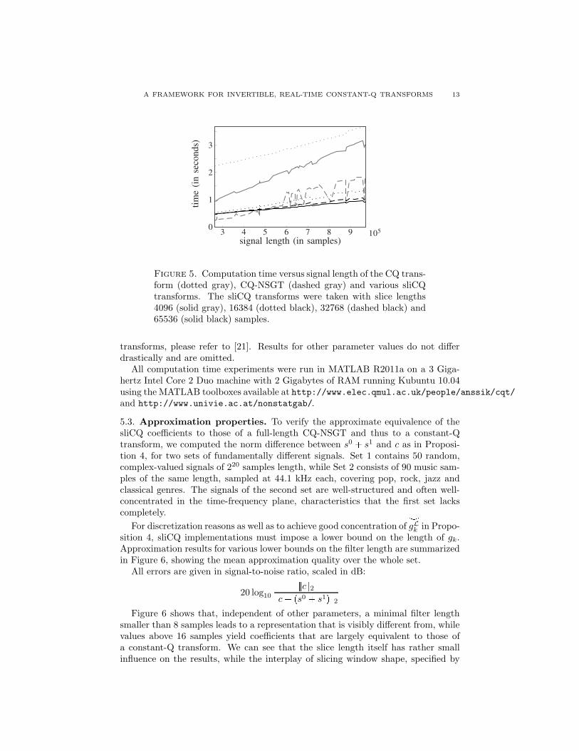
5.2. Performance evaluation. A comparison of the CQ-NSGT algorithm withprevious constant-Q implementations was given in [21]. Figure 4 reproduces andextends some of the results; it shows, for both the constant-Q implementation pro-vided in [18] and CQ-NSGT, mean computation duration and variance for analysisfollowed by reconstruction, against signal length. The plot also illustrates the de-pendence of CQ-NSGT on the prime factor decomposition of the signal length L.

Figure 5 illustrates the performance of sliCQ compared to the constant-Q andCQ-NSGT algorithms shown in Figure 4. Linearity of the sliCQ algorithm be-comes obvious, deviations occurring due to unfavorable FFT lengths 2Nak in(i)CQ-NSGT2N . Performance improvements for increasing slice length can beattributed to the advanced nature of MATLAB’s internal FFT algorithm, as com-pared to the current implementation of the sliCQ framework.

The performance of the involved algorithms does not depend on signal content.Consequently, random signals were used in the performance experiments, althoughwe implicitly assumed the signals to be sampled at 44.1 kHz. All the results repre-sent transforms with 48 bins per octave, minimum frequency 50 Hz and maximumfrequency 22 kHz, in Section 6 a maximum frequency of 20 kHz is used instead.For a more comprehensive comparison of the CQ-NSGT to previous constant-Q


3 4 5 6 7 8 9¢ 105

0

1

2

3

signal length (in samples)

time(inseconds)

Figure 5. Computation time versus signal length of the CQ trans-form (dotted gray), CQ-NSGT (dashed gray) and various sliCQtransforms. The sliCQ transforms were taken with slice lengths4096 (solid gray), 16384 (dotted black), 32768 (dashed black) and65536 (solid black) samples.

transforms, please refer to [21]. Results for other parameter values do not differdrastically and are omitted.

All computation time experiments were run in MATLAB R2011a on a 3 Giga-hertz Intel Core 2 Duo machine with 2 Gigabytes of RAM running Kubuntu 10.04using the MATLAB toolboxes available at http://www.elec.qmul.ac.uk/people/anssik/cqt/and http://www.univie.ac.at/nonstatgab/.

5.3. Approximation properties. To verify the approximate equivalence of thesliCQ coefficients to those of a full-length CQ-NSGT and thus to a constant-Qtransform, we computed the norm difference between s0 s1 and c as in Proposi-tion 4, for two sets of fundamentally different signals. Set 1 contains 50 random,complex-valued signals of 220 samples length, while Set 2 consists of 90 music sam-ples of the same length, sampled at 44.1 kHz each, covering pop, rock, jazz andclassical genres. The signals of the second set are well-structured and often well-concentrated in the time-frequency plane, characteristics that the first set lackscompletely.

For discretization reasons as well as to achieve good concentration of|gLk in Propo-sition 4, sliCQ implementations must impose a lower bound on the length of gk.Approximation results for various lower bounds on the filter length are summarizedin Figure 6, showing the mean approximation quality over the whole set.

All errors are given in signal-to-noise ratio, scaled in dB:

20 log10c2

c ps0 s1q2

Figure 6 shows that, independent of other parameters, a minimal filter lengthsmaller than 8 samples leads to a representation that is visibly different from, whilevalues above 16 samples yield coefficients that are largely equivalent to those ofa constant-Q transform. We can see that the slice length itself has rather smallinfluence on the results, while the interplay of slicing window shape, specified by

http://www.elec.qmul.ac.uk/people/anssik/cqt/

http://www.univie.ac.at/nonstatgab/


5 10 15 20 25 30

0

20

40

60

80

100

dB-SNR

0

20

40

60

80

100dB-SNR

Minimal filter length (in samples)

Figure 6. SliCQ coefficient approximation error against the min-imal admissible bandwidth for Set 1 (top) and Set 2 (bottom). Alltransforms use Blackman-Harris windows in the CQ-NSGT step.Solid and dashed lines represent long (14 slice length) and short(1128 slice length) transition areas respectively, while colors cor-respond to the slice length: 4096 (light gray), 16384 (dark gray)and 65536 samples (black).

the ratio of transition area length to slice length, and minimal filter length is illus-trated nicely; remarkably, this ratio influences the approximation quality mainlyfor moderately well localized filters. This is in correspondence with the character-ization given in (12): the circular overspill, given by the second term of the righthand side in (12), depends on the shape and support of the sum of two adjacentslicing windows, in particular for moderately well localized filters. If the windowsare very well localized, the overspill is small independent of the particular shape ofthe slicing area. On the other hand, very badly localized windows make the distinctinfluence of the slicing windows negligible. Finally, a comparison of the top andbottom graphs in Figure 6 shows that the approximation quality is largely inde-pendent of the signal class. For Set 1 the variance is generally negligible ( 0.1 dB)and was omitted. Despite some outliers in Set 2, we have found the approximationquality to depend on the minimal filter length in a stable way, cf. Figure 7. Theseoutliers can be attributed to signals particularly sparse (smaller error) or dense

(larger error) in low frequency regions, where |gLk is least concentrated.

6. Experiments on Applications

Experiments in [21] show how the CQ-NSGT can be applied in the processingof signals taking advantage of the logarithmic frequency scaling and the perfectreconstruction property. In particular, the transposition of a harmonic structure


20 40 60 8020

60

100

dB-SNR

signal

Figure 7. Coefficient approximation error (12) for all signals fromSet 2 and slice and transition length of 65536, resp. 16384 sam-ples. Line style indicates the minimal filter length: 8 (dotted), 16(dashed) and 32 (solid) samples.

time (seconds)

frequency

(Hz)

Transient mask

0 0.5 1 1.5

800

3200

12800

time (seconds)

frequency

(Hz)

Sinusoidal mask

0 0.5 1 1.5

800

3200

12800

Figure 8. Masks for extracting a transient (top) and sinusoidalcomponent (bottom) of the Glockenspiel signal. The gray levelplot describes the amplitude of the mask, with black and whiterepresenting 1 and 0, respectively.

amounted to just a translation of the spectrum along frequency bins, while themasking of the CQ-NSGT coefficients allowed for the extraction or suppression ofa component of the signal. In our experiment, we show that the two procedurescan be used to modify a portion of a signal.


time (seconds)

freq

uenc

y (H

z)

Original Glockenspiel signal

0 0.5 1 1.5

800

3200

12800

time (seconds)

freq

uenc

y (H

z)

CQ−NSGT modified signal

0 0.5 1 1.5

800

3200

12800

Figure 9. CQ-NSGT spectrograms showing an excerpt of theGlockenspiel signal before (top) and after transposition of a com-ponent (bottom).

Figure 8 shows masks for isolating a transient part and the corresponding sinu-soidal part of a Glockenspiel signal, created using an ordinary image manipulationprogram. Therein, the layers paradigm has been used to be able to quickly switchon and off the masks in order to accurately adapt them to the CQ-NSGT repre-sentation of the audio. An “inverse mask” is also constructed for the remainderpart of the signal, essentially decomposing the signal into transient, sinusoidal andbackground portions. The masks have been drawn in the logarithmic domain, to beable to handle the dynamics of the audio. They are linearly scaled in dB units, sothat 0 in the mask corresponds to 105 (100 dB) and 1 corresponds to 1 (0 dB).

While keeping the transient part, the isolated sinusoidal component of the signalis transposed upward by 2 semitones, corresponding to 8 frequency bins. Thetransient, the remainder, and the modified sinusoidal coefficients are then addedand the inverse transform is applied to obtain the resulting processed signal. Forease of use, this process is done with a rectangular representation of the slices,obtained by choosing Lak constant for all frequency bands which corresponds toa sinc-interpolation of the coefficients.

Figure 9 compares the CQ-NSGT spectrograms of the original and the modifiedsignal, while Figure 10 shows the results for the same experiment using sliCQ


transforms with different slice lengths. Note that the plots show the spectro-gram of the synthesized signal, not the time-frequency coefficients before synthe-sis. Further, the exact same mask was used for CQ-NSGT and sliCQ transposi-tions. The sound files for this and other transposition experiments are available athttp://www.univie.ac.at/nonstatgab/slicq. A script for the Python toolboxthat executes the experiment, is available on the same page.

For synthesis, performed from modified coefficients, as opposed to mere recon-struction, an evaluation of the results is a highly non-trivial matter. This is due tothe lack of a properly defined notion of accuracy or the existence of a target signal,not only for the algorithms presented here, but for any analysis/synthesis based sig-nal processing framework. Thus, while the examples in this section should indicatethat CQ-NSGT synthesis and sliCQ synthesis can produce results in accordancewith intuition, an in-depth treatment of this subject is far beyond the scope of thisarticle.

7. Summary and Conclusion

In this contribution, we have introduced a framework for real-time implementa-tion of an invertible constant-Q transform based on frame theory. The proposedframework allows for straight-forward generalization to other non-linear frequencyscales, such as mel- or Bark scale, cp. [9]. While real-time processing is possibleby means of a preprocessing step, we investigated the possible occurrence of time-aliasing. We provided a numerical evaluation of computation time and quality ofapproximation of the true NSGT coefficients.

In analogy to the classical phase vocoder, phase issues have to be addressed,if CQ-transformed coefficients are processed, cp. [12, 13, 17]. While preliminaryexperiments using the proposed framework for real-life signals were presented, un-desired phasing effects, mainly due to the contribution of a signal component toseveral adjacent filters, will be investigated in detail in future work. Furthermore,future work will consider the efficient realization of adaptivity in both time andfrequency by varying the length of the preprocessing windows used for slicing.

8. Appendix

8.1. Derivation of CQ-NSGT properties.

Proof of Proposition 1. By Algorithm 1, we have

cn,k ckrns

a

Lak1

Lak

Lak1¸

m0

ak1¸

l0

pf gkqrm lL

akse2πinmakL

Lak1¸

m0

ak1¸

l0

pfMnakgkqrm l

L

aks(13)

Since Lak ¥ L, only one element of the inner sum above is non-zero, for eachm P t0, . . . , Lal 1u. It follows that

(14) cn,k xf ,Mnak

gky.

http://www.univie.ac.at/nonstatgab/slicq


time (seconds)

freq

uenc

y (H

z)

sliCQ modified signal, long slice

0 0.5 1 1.5

800

3200

12800

time (seconds)

freq

uenc

y (H

z)

sliCQ modified signal, short slice

0 0.5 1 1.5

800

3200

12800

Figure 10. sliCQ spectrograms showing an excerpt of the Glock-enspiel signal after transposition of a component. The top plot wasdone with a slice length of 50000 and a transition area of 20000samples, the bottom plot with a slice length of 5000 and a transi-tion area of 2000 samples.

Inserting into Algorithm 2 yields, for all j P t0, . . . , L 1u,

ˆf rjs

¸

kPIK

Lak1¸

n0

cn,ke2πinmakL

rgkrjs

¸

kPIK

Lak1¸

n0

xf ,Mnak

gkyMnakrgkrjs,

the discrete frame synthesis formula. By assumption, Gpg, aq and Gpg, aq are dualNSG frames and thus

ˆf rjs frjs, for all j P t0, . . . , L 1u.

Applying the inverse discrete Fourier transform completes the proof.


Proof of Proposition 2. Denote by Jk an interval of length Lk, Lk as in Section 2,containing the support of gk. By assumption

0 ¸

kPIK

|gkrjs|2 8, for all j 0, . . . , L 1

and Lak ¥ Lk |Jk|. Note that the frame operator (2) can be written as follows

Sf rjs ¸

kPIK

Lak1¸

n0

xf,MnagkyMnagkrjs

¸

kPIK

L

ak

Lak1¸

n0

IFFTLakpfgkqrnsgkrjse

2πinjakL

¸

kPIK

L

akFFTLak

pIFFTLakpfgkqqrjsgkrjs,(15)

for all f P CL. Furthermore, with χJkthe characteristic function of the interval Jk,

fgk χJk

ak1¸

l0

TlLakpfgkq

χJkFFTLak

pIFFTLakpfgkqq

and, obviously, gk χJkgk. Inserting into (15) yields

Sf rjs ¸

kPIK

L

akpfgkqrjsgkrjs

f rjs¸

kPIK

L

ak|gk|

2rjs.(16)

With the sum bounded above and below, the inverse frame operator can be writtenas

(17) S1f rjs f rjs

¸

kPIK

L

ak|gk|

2rjs

1

, for all f P CL.

Since the elements of the canonical dual frame are given by (3), this completes theproof.

8.2. Derivation of sliCQ properties.

Proof of Proposition 3. According to Proposition 1, fm, the output of iCQ-NSGTin Step 9 of Algorithm 4 satisfies to fm

rjs pf TmNh0qrj pm 1qN s. Since°

m TmN

h0h0

1 holds,

f

¸

m

pf TmNh0qTmN h0 f ¸

m

TmN

h0h0

f

follows.


Proof of Proposition 4 . Since gk is obtained by sampling gLk with sampling periodL2N , the (inverse) Fourier transform qgk of gk is given by periodization of gLk asfollows:

(18) qgkrls

L2N

1¸

j0

|gLk rl j 2N s.

Recall from (6) that the CQ-NSGT coefficients of f with respect to GpgL, aq are

given by cn,k xf,Tnak

|gLk y, while the CQ-NSGT coefficients cm of fm are, for

m 0, . . . , LN 1, ns 0, . . . , 2N

ak 1 and k P IK

cmns,k x

xfm, gns,ky x

xfm,Mnsak

gky

xfm,Tnsakqgky

C

f, hm

L2N

1¸

j0

Tnsakpm12jqN|gLk

G

,(19)

where the final inner product is taken over CL. Observe that every n 0, . . . , Lak1

can be written as n m Nak

ns with ns from 0, . . . , Nak

1 and thus

s0n,k s1n,k cmnsNak,k

cm1ns,k

C

f, phm hm1q

L2N

1¸

j0

Tnsakpm2jqN|gLk

G

A

f,TnsakmN|gLk

E

Rrns

A

f,TakpmNak

nsq

|gLk

E

Rrns

cn,k Rrns.(20)

Here,

Rrns A

f, p1 hm hm1qTnsakmN|gLk

E

C

phm hm1q

L2N

1¸

j1

Tnsakpm2jqN|gLk

G

.(21)

Hence s0n,ks1n,k cn,k Rrns. The result follows from Cauchy-Schwartz’ inequal-ity, applied to the case m 0, observing independence from m.

Acknowledgment

This research was supported by the WWTF project Audio-Miner (MA09-024),the Austrian Science Fund (FWF):[T384-N13] and the EU FET Open grant UN-LocX (255931). The authors wish to thank the reviewers for their extremely helpfuland constructive remarks on the first version of the manuscript.

References

[1] P. Balazs, M. Dorfler, F. Jaillet, N. Holighaus, and G. A. Velasco, “Theory, implementationand applications of nonstationary Gabor Frames,” J. Comput. Appl. Math., vol. 236, no. 6,p. 14811496, 2011.


[2] J. Brown, “Calculation of a constant Q spectral transform,” J. Acoust. Soc. Amer., vol. 89,no. 1, p. 425434, 1991.

[3] J. C. Brown and M. S. Puckette, “An efficient algorithm for the calculation of a constant Qtransform,” J. Acoust. Soc. Am., vol. 92, no. 5, pp. 2698–2701, 1992.

[4] A. Chebira and J. Kovacevic, “Life Beyond Bases: The Advent of Frames (Part I),” IEEESignal Processing Magazine, vol. 24, no. 4, pp. 86–104, 2007.

[5] M. Cranitch, M. Cychowski, and D. FitzGerald, “Towards an Inverse Constant Q Transform,”In Audio Engineering Society Convention 120, 5 2006.

[6] I. Daubechies, A. Grossmann, and Y. Meyer, “Painless nonorthogonal expansions,” J. Math.Phys., vol. 27, no. 5, pp. 1271–1283, May 1986.

[7] M. Dolson, “The phase vocoder: a tutorial,” Computer Musical Journal, vol. 10, no. 4, pp.11–27, 1986.

[8] R. J. Duffin and A. C. Schaeffer, “A class of nonharmonic Fourier series.” Trans. Amer.Math. Soc., vol. 72, pp. 341–366, 1952.

[9] G. Evangelista, M. Dorfler, and E. Matusiak, “Phase Vocoders With Arbitrary Fre-quency Band Selection,” in Proceedings of the 9th Sound and Music Computing Conference(SMC’12), Copenhagen, July 2012.

[10] H. G. Feichtinger and T. Strohmer, Gabor Analysis and Algorithms. Theory and Applications.Boston: Birkhauser, 1998.

[11] F. Jaillet, “Representation et traitement temps-frequence des signaux audionumeriques pourdes applications de design sonore,” Ph.D. dissertation, Universite de la Mediterranee - Aix-Marseille II, 2005.

[12] J. Laroche and M. Dolson, “Phase-vocoder: about this phasiness business,” IEEE ASSPWorkshop on Applications of Signal Processing to Audio and Acoustics 1997, pp. 4, October1997.

[13] J. Laroche and M. Dolson, “Improved phase vocoder time-scale modification of audio,” IEEETransactions on Speech and Audio Processing, vol. 7, no. 3, pp. 323-332, May 1999.

[14] J. Li, T. Nguyen, and S. Tantaratana, “A simple design method for near-perfect-reconstruction nonuniform filter banks,” IEEE Transactions on Signal Processing, vol. 45,no. 8, 1997.

[15] R. Marks, Handbook of Fourier Analysis and its Applications. Oxford University Press,2009.

[16] K. Nayebi, I. Barnwell, T.P., and M. Smith, “Nonuniform filter banks: a reconstruction anddesign theory,” IEEE Transactions on Signal Processing, vol. 41, no. 3, 1993.

[17] J. Roe, Lectures on Coarse Geometry, ser. University Lecture Series. Providence, RI: Amer-ican Mathematical Society, 2003, vol. 31.

[18] C. Schorkhuber and A. Klapuri, “Constant-Q toolbox for music processing,” in Proceedingsof 7th Sound and Music Computing Conference (SMC’10), Barcelona, July 2010.

[19] I. Selesnick and I. Bayram, “Frequency-domain design of overcomplete rational-dilationwavelet transforms,” IEEE Trans. Signal Process., vol. 57, no. 8, pp. 2957–2972, 2009.

[20] J. O. Smith, “Audio FFT Filter Banks,” in Proceedings of 12th International Conference onDigital Audio Effects (DAFx-09), Como, September 2009.

[21] G. A. Velasco, N. Holighaus, M. Dorfler, and T. Grill, “Constructing an invertible constant-Qtransform with non-stationary Gabor frames,” in Proceedings of 14th International Confer-ence on Digital Audio Effects (DAFx-11), Paris, September 2011.

[22] J. Youngberg and S. Boll, “Constant-Q signal analysis and synthesis,” In IEEE InternationalConference on Acoustics, Speech, and Signal Processing (ICASSP ’78), volume 3, pages 375– 378, 1978.


Acoustics Research Institute, Austrian Academy of Sciences, Wohllebengasse 12-14,1040 Vienna, Austria

E-mail address, Nicki Holighaus: [email protected]

Numerical Harmonic Analysis Group, Faculty of Mathematics, University of Vienna,Alserbachstraße 23, 1090 Vienna, Austria

E-mail address, Monika Dorfler: [email protected]

Institute of Mathematics, University of the Philippines-Diliman, 1101 Quezon City,Philippines

E-mail address, Gino Angelo Velasco: [email protected]

Austrian Research Institute for Artificial Intelligence, Freyung 6/6, 1010 Vienna,Austria

E-mail address, Thomas Grill: [email protected]

Documents

A FRAMEWORK FOR INVERTIBLE, REAL-TIME ... FRAMEWORK FOR INVERTIBLE, REAL-TIME CONSTANT-Q TRANSFORMS NICKI HOLIGHAUS, MONIKA DORFLER, GINO ANGELO VELASCO,¨ AND THOMAS GRILL Abstract