A Framework for Modelling Interaction Between

Ecological and Economic SystemsThis version: January 5th, 2001

Shunli Wang1

Peter Nijkamp1

Erik Verhoef1

Keywords: economic-ecological interaction, spatial externality

Abstract

Transboundary environmental issues, like climate change, have in recent years received much

attention from the side of political scientists and economists. Within the economics discipline,

we witness sometimes differences between ecologically-oriented and mainstream economists,

which may form a barrier for proposing clear policy recommendations on external effects in

open and interacting spatial systems. This unfortunate situation may be due to lack of an

integrated analytical framework as well as to the multi-disciplinarity of the problem at hand.

The present paper aims to identify some relevant aspects for a methodological synthesis for

analysing sustainable development issues in open economic systems with a view to the

development of an integrative framework through which a great many ecological-economic

studies can be investigated. We focus on conceptual issues centring around the integration on

interacting economic and ecological subsystems, inter alia in relation to spatial externalities

and ecological footprints. Our discussion enables us to build a framework for a systematic

categorisation of various types of models for economic-ecological interaction. The paper

concludes with some reflections on the way forward.

Pn960SWEV

1 The authors are affiliated with the Free University, Amsterdam, Department of Spatial Economics, De Boelelaan 1105, NL-1081 HV Amsterdam, The Netherlands. Corresponding author: phone number: (+)31-20-4446142; email: swang@econ.vu.nl.

1. Introduction

Transboundary environmental issues have received increased attention from

contemporary environmental policy-making institutions. One of the examples is the

United Nations Framework Convention on Climate Change and the corresponding

Kyoto Protocol. From a scientific point of view, the study of transboundary

environmental issues is, among other things, interesting because of its

multidisciplinary character. Analysing these problems may lead to a better

understanding of, and synergy between, various disciplines, which might result in

significant scientific benefits from an interdisciplinary perspective. A drawback of

multidisciplinarity is, however, that some of the integrated perspectives may be

disputed on specific monodisciplinary grounds. For example, from an economic point

of view, there may be a tension between ecological economics and mainstream (neo-

classical) economics. Given the criterion of ‘consilience’, recently introduced by

Wilson (1998) and meaning that the methods and starting points of one scientific

discipline need to be consistent with the accepted insights of other disciplines (see

Van den Bergh 2000), this tension is unfavourable and would have to be relaxed.

Lack of coherence between these two dominant orientations in economics,

henceforth denoted as mainstream and ecological perspectives respectively, seems to

create a problematic situation. In particular, the ecological perspective is often seen as

a fundamental critique on the mainstream perspective, especially regarding its failure

in explaining and offering possibilities for correcting the severe and sometimes

irreversible environmental degradation (for a review, see e.g. Van den Bergh 1996,

Spash 1999). The feeble position of mainstream economics became in particular

evident after the optimism in the 1960s and beyond (as expressed e.g. by the concept

of the golden rule of accumulation), and notably in the destruction of the growth

optimism by the Report of the Club of Rome (Meadows et al. 1972) and the

subsequent increasing political popularity of the concept of sustainable development.

It became gradually clear that the ecological system would have to be recognised as

an integral entity - in addition to the economic system - in analysing environmental

scarcity problems.

This paper aims to bring both perspectives together by putting the various

models in terms of both above-mentioned perspectives in a unifying framework.

Furthermore, we will illustrate this framework by presenting and discussing a spatial-

economic model with environmental interactions for economic activities, markets and

- 1 -

externalities, followed by a discussion of ecological footprint issues in terms of

transboundary externalities.

The plan of this paper is as follow. Section 2 first discusses conceptual

differences as well as similarities between the mainstream and ecological perspectives

in analysing environmental issues; next, this section presents a unifying modelling

framework for the interaction between relevant economic and ecological systems.

Section 3 reviews and interprets various models, which are based on either

perspective, in terms of the above-mentioned unifying framework in order to identify

compatibilities between both perspectives. Section 4 illustrates the insights thus

obtained by discussing (i) insights from a spatial model on transboundary

externalities, firms and markets, as well as (ii) the ecological footprint in terms of

transboundary externalities. Finally, section 5 offers some concluding research

remarks.

2. A Modelling Framework for Ecological and Economic Interaction

2.1 The clash of ideas: economic versus ecological perspective

In this section we will concisely discuss both a mainstream, conventional economic

and an ecological economic perspective. The fundamental concepts in the field of

environmental economics – as part of mainstream economics – are the ‘externality’

and ‘public goods’ character of environmental amenities (Baumol and Oates 1975). In

economic analysis, an externality is generally conceived of as a divergence between

the marginal social and private cost of a good. Environmental damage thus typically

involves a negative externality, when it is not (or not optimally) priced. The result is

that a tax, subsidy or other governmental measure is justified in order to correct the

impact of such an externality (Verhoef 1999). This description of an externality

implies thus that (i) an externality exists when some agents’ action influences the

utility of other agents, without this effect being reflected in price signals (see e.g.

Mishan 1971), and (ii) necessary conditions for a socially optimal situation (i.e., the

Pareto-optimality conditions) are violated (Buchanan and Stubblebine 1962, Baumol

and Oates 1975, Mas-Colell et al. 1995).

Although the concept of externality is widely used, various definitions still

exist (Viner 1930, Mishan 1971, Meade 1973, Ng 1988), while some of them may be

imprecise (as observed by Mas-Colell et al. 1995). This may be one reason why the

concept of externality is not always clear to a non-economist (Sterner and Van den

Bergh 1998). A fallacious loose interpretation would be that the ecological system can - 2 -

be considered as external to an economic system and ‘therefore’ irrelevant for

economic efficiency (see for a review e.g. Van den Bergh 1996, Sterner and Van den

Bergh 1998). This interpretation of externality is obviously missing the point, since

the use of the externality concept implies, on the contrary, that the ecological system

does matter to economic efficiency.

The ecological perspective emphasises that economic growth will result in an

increased use of natural resources or increased damage to ecological systems as a

result of pollution, even when externalities are optimised (Meadows et al. 1972; Daly

1990, 1997c). More specifically, sustainable growth from a mainstream economic

perspective (Solow 1974 and Hartwick 1977) may even have a different interpretation

(Common and Perrings 1997) than the concept of 'sustainable development' from an

ecologically-oriented economic perspective (Holling 1973). That is, even when

increasing scarcity of an environmental good would be coped with by an increase in

environmental taxes – or, more broadly, in taxes that would in addition reflect

intergenerational equity considerations (Withagen 1995, 1996) –, the outcome may

still not be regarded as strictly sustainable (over an infinitely long time frame). This

conclusion derives from the assumption that the earth is a closed system, as well as

from the laws of thermodynamics. These laws play important roles in the ecological

perspective (Van den Bergh 2000).

The first law of thermodynamics states that, in a closed ecological system,

energy cannot be created nor destroyed (Georgescu-Roegen 1993). Translated into

economic activities, this law implies that sustainable economic growth is not possible,

as the available energy is given. For instance, the sun will die in around 5 billion years

from now. Moreover, it is questionable whether the energy available from

undepletable sources would be sufficient to satisfy the demand of an imaginary

maximum world population. A further complication from the thermodynamic laws is

that growth inevitably declines if the second law is taken into account. This second

(or ‘entropy’) law states that the entropy in the universe is increasing. Entropy may –

even though the precise notion of entropy is ‘not easily understood’ (Georgescu-

Roegen 1993: 77) – be seen as a measure for the unavailable energy in the system. In

Georgescu-Roegen’s economic terms, this means that “matter/energy enters the

economic process in a state of low entropy, and comes out of it in a state of high

entropy” (Georgescu-Roegen 1993: 77). In other words, the economic process in case

of natural resource use (material or energy) is always a declining process, as the

closed system always changes from low-entropy to high-entropy. Therefore, as - 3 -

Ehrlich et al. (1993: 70) proclaimed, we [even] become worse off as energy flows to

places where we can no longer get at it. These insights suggest that an ‘optimum’

development over an infinitely long time frame may be impossible to define.

In a similar vein, regarding materials use, the concept of ‘material balance’ has

been put forward by ecological economists (Kneese et al. 1970, Ayres 1978, Ruth

1993, Van den Bergh 1996). This means that the same mass of input (material use) in

the economic system, which is extracted from the ecological system, should return as

output of the economic system into the ecological system. This feedback could be

represented by, for example, material waste or pollution. In this interpretation, the

resources are materials that initially have low entropy and become waste, which are

materials of high entropy (Ayres 1999, Van den Bergh 1996).

The supporters of the ecological perspective argue that mainstream economics

is too much ‘value-based’ (see for instance the special issue on this topic in

Ecological Economics of April 1998; Daly 1991, 1998; and Ayres 1998), the main

mainstream message being to get the prices right. Critics emphasise that, following

Georgescu-Roegen’s application (1971) of thermodynamic laws to economics, it

should be the physical quantities rather than economic values that should play a

central role in studying sustainable development (e.g. Rees 1999, Wackernagel 1999a

and Yount 1999). After all, the natural environment is limited in a physical sense

(Daly 1995, 1997a, b, Ayres 1998).

This critique may be challenged on the ground that it seems to be based on a

somewhat restricted representation of the mainstream economic perspective. For one

thing, the ‘wealth of nations’, as well as the possibilities for ever-increasing growth,

have intrigued mainstream economists for centuries already (e.g. Smith, Mill, Keynes,

Samuelson, Solow). The ultimate goal of the ‘homo economicus’ is a quantity-

oriented one – that is, the maximisation of welfare as enjoyed from the consumption

of scarce physical goods, be it ordinary market goods or improperly priced natural

goods (see e.g. Mas-Colell et al. 1995, Samuelson 1947). ‘Consumption’, in this

sense, does not necessarily mean ‘use’: the utility enjoyed from knowing that certain

rare species still exist deep sea can be seen as the consumption of the public good ‘the

existence of that species’. Mainstream environmental economists thus distinguish

‘use’ from ‘non-use’ values (along with further distinctions regarding, for instance,

‘bequest’ values and ‘option’ values)

The same sort of quantity-oriented social utility function applies for the ‘social

planner’ as typically assumed in mainstream economic models. Moreover, economic - 4 -

theory, ever since Adam Smith, shows that the transactions of the utility maximising

economic subjects tend to result in a competitive market equilibrium that is Pareto-

optimal (the ‘First Theorem of Welfare Economics’). Efficient prices are not the

ultimate goal, but only instruments.

Of course, this theorem holds true only under the usual assumptions of

absence of market failures. In case of imperfections and non-optimal outcomes in

environmental issues resulting e.g. from the existence of externalities, due attention

should be paid to the interaction between the economic and the ecological system,

especially if the interactions between and within both systems are complex and non-

linear.

For modelling these interactions, compatibility between both perspectives may

be reached by interpreting the variables concerned in terms of quantities rather than

values. This is not an insurmountable problem, as in the economics literature,

typically only quantity based variables enter private and social utility and production

functions as arguments (see e.g. general-equilibrium theory or micro-economic

theory; for example, Mas-Colell et al. 1995).

On logical grounds, the two approaches would be intrinsically mutually

inconsistent, only if the optimal quantities considered by the ecological perspective

could not be realised by using a system of taxes (e.g. Pigouvian taxes) that is

consistent with the mainstream economic approach. There is however, a priori, no

fundamental and compelling reason why this should be the case. Certainly, practical

pricing of all attributes or elements in an ecological system might hardly be possible,

but in that case we enter the theory of ‘second-best’ environmental taxation. There is

a large and growing mainstream based literature on this, emphasising the economic

aspects of relaxing various simplifying assumptions that, while keeping exposition

manageable, often give standard mainstream economic models a somewhat abstract

and conceptual nature (e.g. Verhoef and Nijkamp, 1999).

In conclusion, insights from an ecological-economic perspective raise the

question of whether flows of inputs necessary to achieve a sustainable development in

terms of production and consumption flows (the one side of the coin) can be extracted

from intrinsically finite stocks with bounded regeneration over an infinitely long time

span and for a possibly permanently growing world population, while keeping

environmental quality at an acceptable (‘sustainable’) level (the other side of the

coin). The emphasis on the (very) long run can, in a way, be seen a warning against

the mainstream economic practice of discounting future utility (related also to - 5 -

environmental quality), which tends to leave such questions to practically zero

importance in intertemporal optimisation exercises. An immediate objection against

such a critique would be that nothing prevents a mainstream economist from

proposing different objectives and/or constraints, which would more explicitly reflect

these worries. One possibility, studied for instance by Withagen (1996), is that utility

per capita may be restricted to be ‘non-decreasing over time- possibility’ after

allowing for some transitional phase.

2.2. Integrated economic-ecological systems

An integrated framework

The conceptual differences and similarities between both perspectives may be

clarified by putting the underlying models in a unifying framework. In this subsection,

we will present such a framework for modelling the interaction between ecological-

economic systems, which serves as the basis for discussing a number of approaches in

the literature aimed to study the relations between economic and ecological systems.

We focus on two particular aspects of the debate only, namely (1) the use of quantity

versus value based measures and (2) the degree of integration between the economic

and ecological sub-systems. By using this integrative framework, some of the

methodological differences between both perspectives previously discussed turn out

to be non-fundamental, but mainly a matter of choice of objective. Furthermore,

positioning the economic and ecological perspectives in terms of a ‘system’ will show

that the concept of quantity may in fact be a strong link between the ecologically-

oriented perspective and the mainstream models, in which consumption is the amount

that is transformed from the inputs and where the price of consumption reflects the

consumers’ marginal value of goods. As will be shown, the result of this framework

may also be associated with relevant complementary approaches such as the material

balance model (see e.g. Van den Bergh 1991, 1996; Van den Bergh and Nijkamp

1994).

In the framework proposed here, we will consider the ecology and the

economy as an integrated system. Here we will follow Bossel (1986), who used the

term system as a means “to describe a set of components interacting relatively

strongly with each other and relatively weakly with their common environment, in a

way which allows one to recognize a ‘purpose’ in the resulting overall behavior of the

interacting components” (p. 51). In the context of our paper, the following four

starting points are taken for granted: (i) the social objective in general is increasing in - 6 -

the ‘quality of life’ at all relevant points in time, and may take various forms, such as

the requirement that the average quality of life should not decline over a given long-

term horizon, or – more traditional – that the discounted net present value of the

quality of life be maximized; (ii) a system is composed of well-defined elements,

which are identified by focussing on the most essential simplification of the system;

(iii) a system has a structure that represents the interaction between the elements; and

(iv) a system has its boundary which separates it from the system environment (in our

case, we study the integration of an economic and ecological system only).

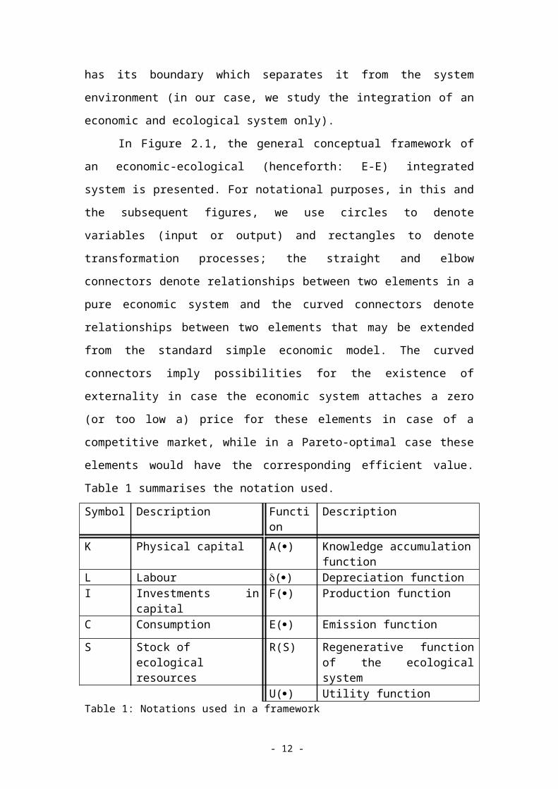
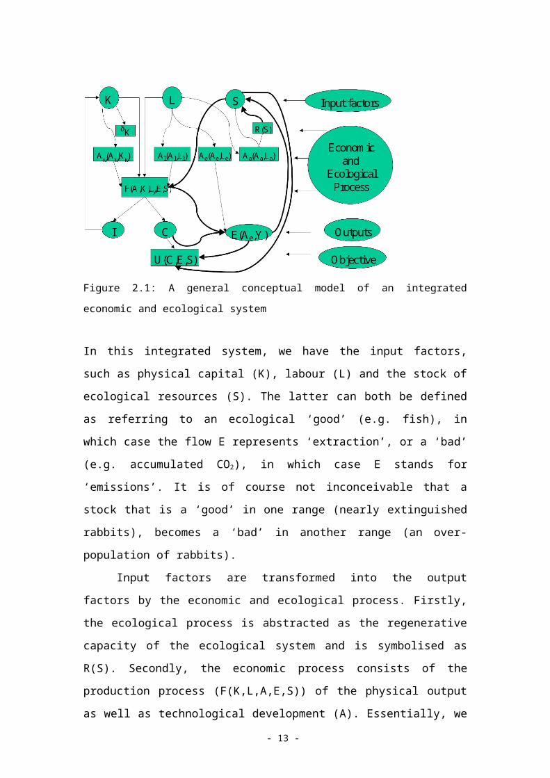
In Figure 2.1, the general conceptual framework of an economic-ecological

(henceforth: E-E) integrated system is presented. For notational purposes, in this and

the subsequent figures, we use circles to denote variables (input or output) and

rectangles to denote transformation processes; the straight and elbow connectors

denote relationships between two elements in a pure economic system and the curved

connectors denote relationships between two elements that may be extended from the

standard simple economic model. The curved connectors imply possibilities for the

existence of externality in case the economic system attaches a zero (or too low a)

price for these elements in case of a competitive market, while in a Pareto-optimal

case these elements would have the corresponding efficient value. Table 1

summarises the notation used.

Symbol Description Function DescriptionK Physical capital A() Knowledge accumulation

functionL Labour () Depreciation functionI Investments in capital F() Production functionC Consumption E() Emission function

S Stock of ecological resources

R(S) Regenerative function of the ecological system

U() Utility functionTable 1: Notations used in a framework

- 7 -

Figure 2.1: A general conceptual model of an integrated economic and ecological system

In this integrated system, we have the input factors, such as physical capital (K),

labour (L) and the stock of ecological resources (S). The latter can both be defined as

referring to an ecological ‘good’ (e.g. fish), in which case the flow E represents

‘extraction’, or a ‘bad’ (e.g. accumulated CO2), in which case E stands for

‘emissions’. It is of course not inconceivable that a stock that is a ‘good’ in one range

(nearly extinguished rabbits), becomes a ‘bad’ in another range (an over-population of

rabbits).

Input factors are transformed into the output factors by the economic and

ecological process. Firstly, the ecological process is abstracted as the regenerative

capacity of the ecological system and is symbolised as R(S). Secondly, the economic

process consists of the production process (F(K,L,A,E,S)) of the physical output as

well as technological development (A). Essentially, we could distinguish four forms

of technological developments: basic knowledge (Ak), human capital knowledge (Al),

knowledge on efficient emission technology (Ae) and knowledge on efficient

abatement technology (Aa). The developments of these knowledge systems depend on

the existing knowledge level as well as on extra input in the form of capital and/or

labour (in which case ‘endogenous growth theory’ comes into play). Finally, we have

to face also the depreciation of physical capital (k) that could be the result of either

economic or ecological processes. Note that the figure ignores the possibility of

depreciation of knowledge.

The input factors are, via the economic and ecological process, transformed

into outputs. The outputs consist of (i) investments, (ii) consumption and (iii)

emission. Emission as well as investments have a feedback function. Consumption is - 8 -

one of the main elements in the valuation process from an economic perspective. The

social objective in this integrated system is the utility from consumption (positive),

emission (negative) or extraction, and the valuation of the state of the ecological

system (changes in which may be either positive or negative depending on whether it

is an improvement or deterioration).

Temporal and spatial dimensions

In representing the interaction framework between an economic and ecological

system as a conceptual model in the form of Figure 2.1, we made an implicit choice

for the objective, elements, structure and boundary of the system. This conceptual

framework may, however, be extended with temporal and spatial dimensions, which

are essential in many contemporary policy issues related to transboundary

environmental issues in a sustainable economy.

The temporal aspect is important as, given the specification of the E-E

interaction system in a static setting, it is still possible for the system to move into

multiple directions of development. In this respect, even in a small model of E-E

interaction, a chaotic system could be simulated in the course of time (see e.g.

Nijkamp and Reggiani 1993). In modelling temporal behaviour, Braat and Lierop

(1987) mention three important aspects, i.e. (i) turnover time, (ii) temporal dynamics

and (iii) temporal development horizon. Temporal development relates to the question

how to determine the total time horizon to be considered. Temporal dynamics relates

to the shape of curves indicating the development of the components, for example, the

stock and regenerative capacity in the ecological system or labour and capital in the

economic system. Finally, turnover time relates to the question whether the total time

horizon should be divided into smaller parts to describe the average lifetime of the

species in case of considering the ecological system as a living system.

In analogy to the time aspects, the spatial dimension is another complicating

factor in modelling the interaction between the economic and the ecological system.

Braat and Lierop (1987) have distinguished here three aspects. First, spatial scale may

differ between both systems; after all, an economic region is rarely the same as an

ecological region. Next, the related spatial development horizon, which refers to the

impacts and development radius, may differ between the systems. For example, a

regional economic activity may cause a multiregional ecological problem (see e.g. the

discussion on ecological footprints, Wackernagel (1999b). Furthermore, various

elements may be mobile over space, which may be relevant for instance for - 9 -

productive inputs (at least capital and labour), outputs, and emissions. Finally, the

analysis becomes even more complicated if we are also dealing with spatial dynamics,

in which case, even without an E-E interaction, a chaotic system might emerge (see

e.g. Nijkamp and Reggiani 1998).

Then, in order to derive analytical or numerical results, the functional form for

the system’s structure should be chosen and a quantification of the parameters should

be given, after the functional specification has been made. Main problems in this step

are in particular caused by the influence of uncertainty. Uncertainties may, as Braat

and Lierop (1987) state, be due to (i) stochastic properties of the system components,

(ii) lack of knowledge, i.e. about system state and processes, (iii) problems of data

measurement and interpretation, (iv) lack of control on various input factors, (v)

limited duration of operationality of control systems and (vi) changing perspectives,

moral standards and values. This observation applies also to the subsequent modelling

attempts.

In extending the conceptual framework in time and space, we would have

more complications to sort out. The difficulty lies not only in the subdivision of the

elements of the system, (e.g. labour, capital, stock and consumption into region

specific components), but also in specifying the relationships between these

components. In terms of space, for example, the production in region A may use the

labour from its own region, but capital from other regions. When combined with the

ecological system, we may have that production in region A may cause a change in

the stock of ecological resources in other regions. Thus, there are many possibilities

when the number of elements as well as the number of regions are large. Therefore,

uncertainties in E-E interacting systems are larger, because we have to consider an

increased number of elements and thus an increased number of structural

relationships.

3. Different Degrees of Integration

In this section, the differences and similarities between both above-mentioned

perspectives are presented in terms of our modelling framework. It turns out that some

differences may be caused by the choice related to the consideration of a valid and

reliable representation of a real-world system on the one hand and simplicity and

analytical tractability on the other hand. For reasons of simplicity, we will here

abstract from temporal and spatial dimensions whenever this is possible and does not

unacceptably limit the analysis.- 10 -

We will classify here different types of models that have been proposed in the

relevant literature by identifying different degrees of integration that can be

distinguished for the two sub-systems. The degree of integration may refer to the four

essential characteristics of the system, i.e. objective, elements, structure and

boundary. We will use here three degrees in terms of structure of the interacting

systems, because the analysis of the structure of a system implicitly determines the

elements and the boundary of the system. Also the objective may be determined by

the structure.

(i) Exogenous constants

In this case, either the effects of the ecological system upon economic productivity

and the utility of economic agents are fully ignored, or the effect of the economic

system upon ecological quality is fully ignored. This impact of the one subsystem on

the other me is at best represented in the parameterisation of the subsystem

considered. In other words, this is the ‘no integration’ case.

(ii) Unilateral interaction

In this case, either the effect of economic activity on ecological indicators or the

effect of ecological indicators on economic productivity and/or utility is taken into

consideration; clearly, with unilateral interaction, no feedback is taken into account.

(iii) Integrated modelling

In this case, there are feedbacks between the two systems, and the behaviour of both

is endogenized. This is clearly the most general type of modelling and the most

preferable one from the viewpoint of realism (note that cases (i) and (ii) are special

cases of (iii)); however, these advantages come at the price of analytical complexity,

which may often prevent closed-form solutions for dynamic optima and other

(equilibrium) paths being available.

Within this category of integrated modelling, one further important distinction can be

made:

(iii-a) Simple integration versus (iii-b) Complex integration

Simple integration will be defined here as a situation where a feedback effect from

sub-system B to A, following a primary effect from A to B, does not lead to changes - 11 -

in sub-system A that will again have an affect on B – whereas with complex

integration, it does. To give an example: suppose we have an economic system that

emits pollution and thus affect the ecological system. If the detoriation of

environmental quality affects utility negatively (because people care about the

environment) but does not lead to changes in consumption and/or production patterns,

we have an instance of simple integration. Complex integration, in contrast, occurs if

the changed ecological conditions lead to either substitution in consumption (for

instance: relocation, defensive behaviour) or changes in production (for instance:

productivity changes in agriculture), which in turn will again have further

environmental implications, in turn inducing further adaptations in the economic

system, etc. In the latter case, there would be an in principle endless sequence of

effects between the two systems, whereas for simple integration, the interaction ends

after the first feedback. Both from a policy perspective and from a modelling

perspective, the difference between the two types of integration is of course

substantial, as a direct result from the different degrees of complexity in the full

system.

3.1 Exogenous constants

Economic subsystem

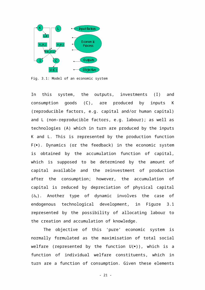
An archetypical economic system might, in the vein of mainstream economic theory,

be described by means of Figure 3.1. In this presentation of the economic system, the

boundary of the economic system is clearly defined. Furthermore, the ecological

system is viewed as exogenous, so that the economic system is fully independent of

the environment. No inputs like natural resources, or outputs like emissions and

pollution, are incorporated explicitly.

K L

I

U(C)

F(Ak,K,L)

C

Input factors

Outputs

EconomicProcess

Objective

Ak(Aa)

k(K)

Al(Al)

Fig. 3.1: Model of an economic system

- 12 -

In this system, the outputs, investments (I) and consumption goods (C), are produced

by inputs K (reproducible factors, e.g. capital and/or human capital) and L (non-

reproducible factors, e.g. labour); as well as technologies (A) which in turn are

produced by the inputs K and L. This is represented by the production function F().

Dynamics (or the feedback) in the economic system is obtained by the accumulation

function of capital, which is supposed to be determined by the amount of capital

available and the reinvestment of production after the consumption; however, the

accumulation of capital is reduced by depreciation of physical capital (k). Another

type of dynamic involves the case of endogenous technological development, in

Figure 3.1 represented by the possibility of allocating labour to the creation and

accumulation of knowledge.

The objective of this ‘pure’ economic system is normally formulated as the

maximisation of total social welfare (represented by the function U()), which is a

function of individual welfare constituents, which in turn are a function of

consumption. Given these elements and structure, the free-market and optimum

growth rates may be determined in various ways (see Romer 1996). In the Ramsey-

Cass-Koopmans formulation, for example, the optimal growth rate is determined by

formulating additional assumptions on given initial endowments K and L, as well as

assumptions on perfect competition. The balanced growth path in the Solow

formulation is derived by the determination of the optimal savings rate, through which

the utility from consumption is optimised (see e.g. Romer 1996). Modern variants

based on endogenous growth theory provides an explanation for an ever-growing

economy by endogenizing the role of investments in technological progress (see e.g.

Aghion and Howitt 1998).

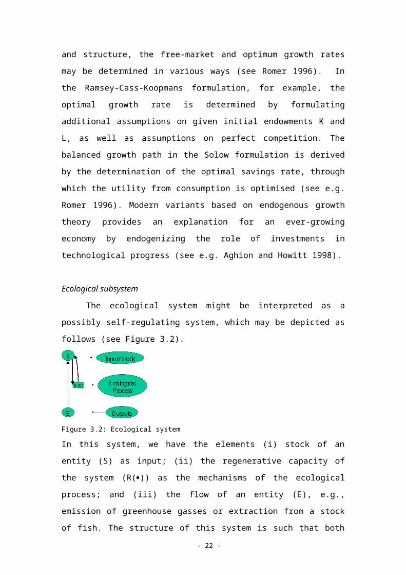
Ecological subsystem

The ecological system might be interpreted as a possibly self-regulating

system, which may be depicted as follows (see Figure 3.2).

Figure 3.2: Ecological system

- 13 -

In this system, we have the elements (i) stock of an entity (S) as input; (ii) the

regenerative capacity of the system (R()) as the mechanisms of the ecological

process; and (iii) the flow of an entity (E), e.g., emission of greenhouse gasses or

extraction from a stock of fish. The structure of this system is such that both the flow

E and the regeneration R(S) affect the stock (S). The simplest way is to model the

regenerative capacity as a function of the stock.

In perceiving the ecological system as a ‘living’ system and subdividing it into

different ecological communities and further specifying it into different populations

that are composed of basic elements, namely the individual, we can interpret

regenerative capacity in terms of birth and death rates of the population. For example,

the birth of the next fish population (R) depends inter alia on the number of the old

population fish stock (S). But, the exact dynamic function might be rather

cumbersome, if one wishes to incorporate the complexities of real-world systems.

In the literature, an unambiguous formulation of an ‘objective’ of the

ecological system – as postulated by mankind; within an ecosystem, each living

species’ ‘objective’ is probably survival – is not easy to find and lies beyond the

scope of this paper. Examples of such an objective may be: biodiversity or

sustainability of the ecological system. The dynamics of the ecological system may

among others include resilience (Holling 1973, Perrings 1998), biodiversity,

compound systems (Clark 1976) or mutualistic systems (Wacker 1999). For a brief

overview of other possibilities of including more complexities in ecological systems,

we refer to e.g. Gowdy and Carbonell (1999).

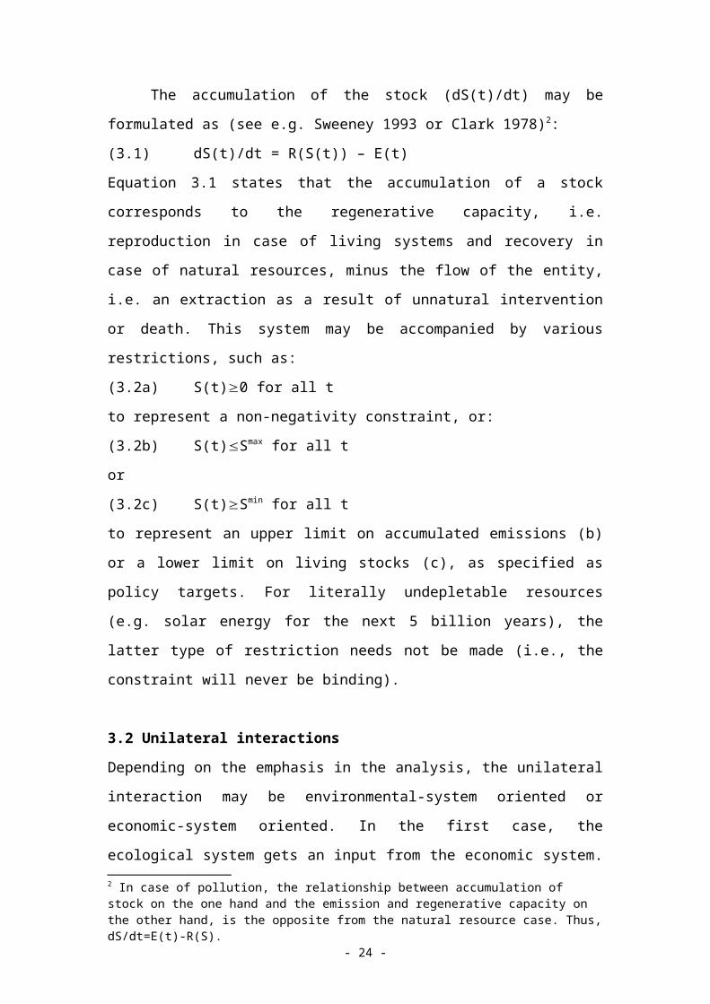
The accumulation of the stock (dS(t)/dt) may be formulated as (see e.g.

Sweeney 1993 or Clark 1978)2:

(3.1) dS(t)/dt = R(S(t)) – E(t)

Equation 3.1 states that the accumulation of a stock corresponds to the regenerative

capacity, i.e. reproduction in case of living systems and recovery in case of natural

resources, minus the flow of the entity, i.e. an extraction as a result of unnatural

intervention or death. This system may be accompanied by various restrictions, such

as:

(3.2a) S(t)0 for all t

to represent a non-negativity constraint, or:

(3.2b) S(t)Smax for all t

2 In case of pollution, the relationship between accumulation of stock on the one hand and the emission and regenerative capacity on the other hand, is the opposite from the natural resource case. Thus, dS/dt=E(t)-R(S).

- 14 -

or

(3.2c) S(t)Smin for all t

to represent an upper limit on accumulated emissions (b) or a lower limit on living

stocks (c), as specified as policy targets. For literally undepletable resources (e.g.

solar energy for the next 5 billion years), the latter type of restriction needs not be

made (i.e., the constraint will never be binding).

3.2 Unilateral interactions

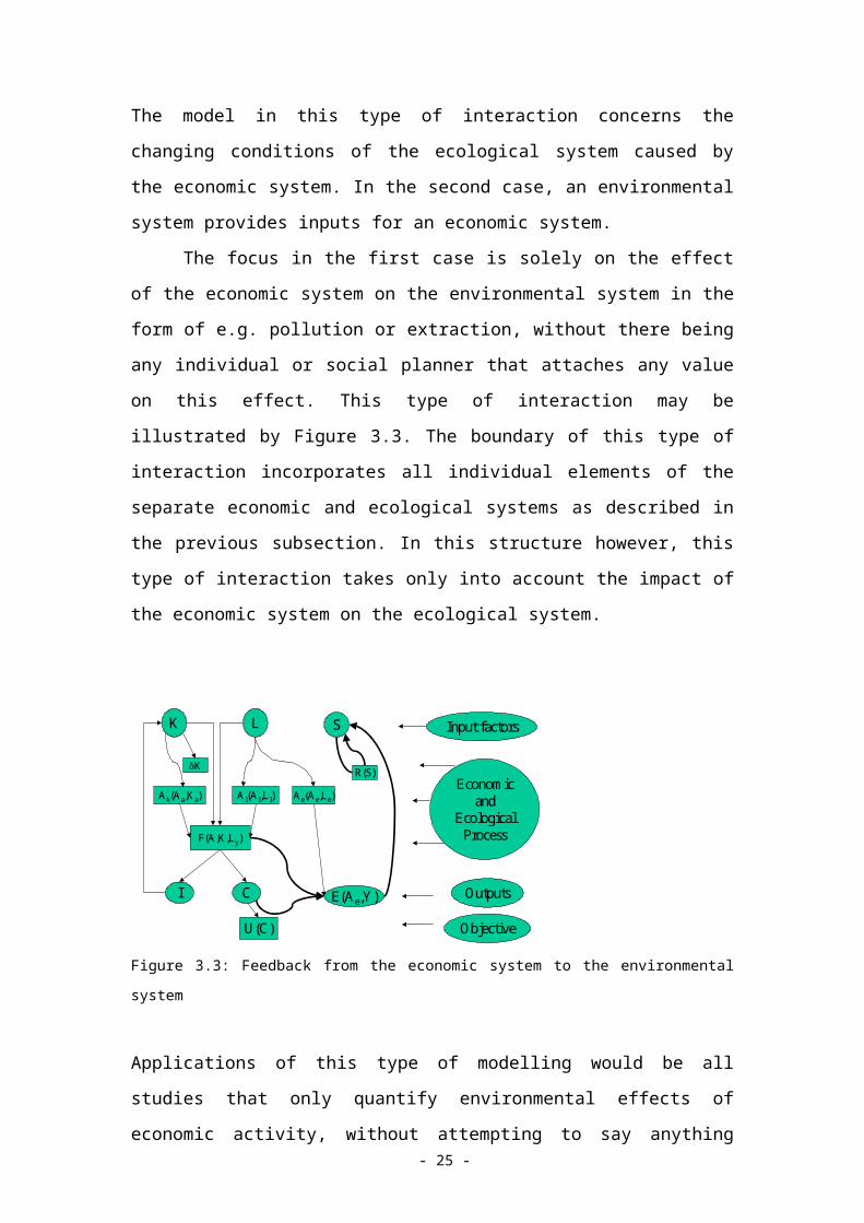
Depending on the emphasis in the analysis, the unilateral interaction may be

environmental-system oriented or economic-system oriented. In the first case, the

ecological system gets an input from the economic system. The model in this type of

interaction concerns the changing conditions of the ecological system caused by the

economic system. In the second case, an environmental system provides inputs for an

economic system.

The focus in the first case is solely on the effect of the economic system on the

environmental system in the form of e.g. pollution or extraction, without there being

any individual or social planner that attaches any value on this effect. This type of

interaction may be illustrated by Figure 3.3. The boundary of this type of interaction

incorporates all individual elements of the separate economic and ecological systems

as described in the previous subsection. In this structure however, this type of

interaction takes only into account the impact of the economic system on the

ecological system.

K SL

I E(Ae,Y)

U(C)

R(S)

F(A,K,Ly)

Ae(Ae,Le)Ak(Aa,Ka) Al(Al,Ll)

Input factors

Outputs

Economicand

EcologicalProcess

Objective

C

K

Figure 3.3: Feedback from the economic system to the environmental system

- 15 -

Applications of this type of modelling would be all studies that only quantify

environmental effects of economic activity, without attempting to say anything about

the social value of such effects. However, most mainstream economic-oriented

literature (Nordhaus 1982, Tahvonen and Kuuluvainen (1991, 1993), Den Butter and

Hofkes 1995, and Van Ewijk and Van Wijnbergen (1995)) in fact do have a feedback

to the economic system via consumption (in the form of waste) or production (in the

form of emission or extraction), or utility in general, so that they may essentially be

categorised as integrated modelling.

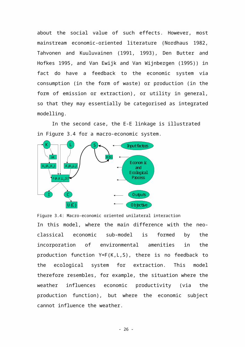
In the second case, the E-E linkage is illustrated in Figure 3.4 for a macro-

economic system.

K SL

I

U(C)

R(S)

F(A,K,Ly,S)

Ak(Ak,Kk) Al(Al,Ll)

Input factors

Outputs

Economicand

EcologicalProcess

Objective

C

K

Figure 3.4: Macro-economic oriented unilateral interaction

In this model, where the main difference with the neo-classical economic sub-model

is formed by the incorporation of environmental amenities in the production function

Y=F(K,L,S), there is no feedback to the ecological system for extraction. This model

therefore resembles, for example, the situation where the weather influences

economic productivity (via the production function), but where the economic subject

cannot influence the weather.

3.3. Integrated modelling

The general case of integrated modelling was already presented in Section 2. This

type of interaction links the individual elements of both ecological and economic

systems and thus also maps out the boundary. However, the structures as well as the

purpose of the resulting E-E interacting system, are presented differently in the

literature. In other words, the feedback linkages are modelled in various ways, namely

via production, consumers’ utility, or both. In this section we will consider such

- 16 -

integrated models, all of which will be in the category of ‘complex integration’ (an

example of simple integration was given in the introduction to Section 3).

Integration via production function

The first case, viz. interaction through feedback by production, may be seen as

complementary to the resource-oriented model, as the price and cost, which are

exogenous in the previous types of model, may then endogenously be determined by

this type of model. An example of the literature that focuses on this relationship can

be found in Clark (1976, chapters 1 and 2). In this case, the objective of the E-E

interacting system is the maximisation of the consumers’ welfare. This type of

interaction may be illustrated by Figure 3.5.

K SL

I E(Ae,Y)

U(C)

R(S)

F(A,K,Ly,S)

Ae(Ae,Le) Aa(Aa,La)Ak(Aa,Ka) Al(Al,Ll)

Input factors

Outputs

Economicand

EcologicalProcess

Objective

C

K

Figure 3.5: E-E interaction via production

Of course, most ecologically-oriented models are more complex, for example, the

climate part of the Dynamic Integrated Climate change and Economy model of

Nordhaus (1994) already takes relationships between carbon emission and

temperature change into account.

A special version of this type of interaction is the natural resource-oriented

studies (Hotelling 1931, Beckmann 1974, Clark 1976, Dasgupta and Heal 1974,

Stiglitz 1974a, 1974b, Prem and Sweeney 1978), where the optimal rate of extraction

or harvesting is investigated on the basis of economic principles. In this literature, the

ecological system is brought back into the ‘economic’ domain (Devarajan and Fisher

1981).

In case of resources, there is the distinction between renewable versus non-

renewable as well as depletable versus non-depletable resources. Depletable resources

typically correspond to the restriction that: S(t) 0 for all t, and S(0) is given (i.e., the

- 17 -

total amount of resources). Non-depletable resources are resources that, by

approximation, are not restricted so that a constrain such as (3.2c) will be a slack one.

Furthermore, the distinction between renewable and non-renewable resources is that

R(S)0 for non-renewable resources (like oil) and R(S)0 for renewable resources

(Sweeney 1993). In terms of E-E systems, this type of interaction implies a

redefinition of the boundary by including an extra element from the economic system

describing the profit from the ecological system (()), depending on the price of the

natural resource (P), the rate of extraction (E) as well as the cost of extraction (())

which in turn depends on the rate of extraction (E) as well as on the amount of the

stock available (S). A graphical illustration of these studies is given in Figure 3.6 and

an example of such a model in terms of extraction of natural resources is found in

Sweeney (1993: 766-767).

S

E

R(S)

(P,E,(S,E))

Figure 3.6: Resource-oriented E-E interaction

The E-E interaction via production model (see Figure 3.5) may partly be rewritten in

terms of a resource-oriented model, as the profit function (()) in the resource-

oriented model is the outcome of the demand from the economic system (see e.g.

Nijkamp 1977). The advantage of writing out the macro-economic sub-model is that

in this way, the price for the stock (as a result of the utility function) as well as the

costs of extraction (embedded in the production function) are endogenously

determined.

Such models are integrated in the sense that profit (or welfare) maximization

determines the optimal speed of extraction and hence the development of the stock

over time, whereas the stock itself may define the profit or welfare optimizing path of

extraction, as well as directly affecting the costs of extraction. Furthermore, such

models may be extended by including the factor human knowledge (A) and other

kinds of resources (M) in the production function; for example, Y=F(A,K,E,M,S) (see

for illustrations e.g. Pezzey 1992, Nijkamp 1977).

- 18 -

Integration via preference function

The second case, viz. modelling mutual interaction by including environmental

factors (E and/or S) in the consumers’ utility function, allows for more analytical

possibilities for modelling the interaction between both systems. This stream of

modelling forms a large part of the literature (see e.g. Thavonen and Kuuluvainen

1991,1993; Byrne 1997, Smulders 1994). The utility function in the context of

environmental issues has usually the following general form (see e.g. Aghion and

Howitt 1998):

max. U(C,S,E)

In this formulation, the emission (E) or the stock of pollution (S) are both amenities,

because both determine the level of utility. The structure of such E-E interacting

system can, depending on the research problem, be presented differently. An example

of a graph of this type of feedback in terms of E-E-interaction is given in Figure 3.7,

where regeneration and technological development are omitted for the ease of

graphical presentation and where the dashed line means that in some models the stock

in ecological systems is not included in the production function.

K SL

I E(Y)

U(C,E,S)

R(S)

F(A,K,Ly)

Input factors

Outputs

Economicand

EcologicalProcess

Objective

C

K

A

Figure 3.7: Integrated modelling in terms of consumers’ utility

As soon as the presence of E and or S as arguments in the utility function induce

behavioural changes due to changes in the ecological sub-system, we have ‘complex

integration’ as defined above.

As pointed out, the most complete E-E interaction is incorporated in the general

model of type Figure 2.1, as it includes all individual elements, structure, boundary as

well as purpose of the systems as discussed in the previous subsections. In Figure 2.1,

interaction is achieved by both consumers’ utility as well as by the production

- 19 -

function. An example of this case is that pollution emission may both affect

consumers’ utility as well as the production because of e.g. health implications. This

model is however rather complicated, as the emission (or stock of resources) in this

case influences the consumers’ utility in two ways, viz. directly via the utility function

and indirectly via the production and thus the consumption. Therefore, it might be

difficult to separate the production or consumers’ effect in empirical modelling. Note

also that when the consumption flows back to the ecological system (via the dashed

line by C and E), this system corresponds to a material balance model (see e.g. Van

den Bergh 1991), as this is a closed system of material flows. Otherwise, the materials

(like waste) remain within the economic system.

4. Spatial Externalities

As argued above, any physical interaction between the economic system and the

ecological system can in principle be evaluated from the perspective of a broadly

defined social welfare function. That is, any possible operational definition of

sustainable development derived on the basis of careful ecological modelling can be

represented in a mainstream framework once one is prepared to include ecological

constraints in the formal welfare maximization formulation. ‘Hard’ physical

constraints would then appear as Lagrangian terms, which will obtain shadow prices

in the (first-best or second-best) constrained optimum, which reflect the marginal

social costs of respecting the constraint. It has been shown (Verhoef, van den Bergh

and Button, 1997) that such shadow prices in a policy context play exactly the same

role as standard mainstream economic marginal external costs. To phrase it otherwise,

any ‘hard’ ecological constraints, however derived, can be translated into a

mainstream economic framework as a vertical marginal external cost function. Hence

our claim that from this perspective, there is not a fundamental impossibility to apply

ecological economics’ physical interpretation of sustainability in a mainstream

oriented policy framework. Doing so has the immediate advantage that the

constrained optimization framework will guide us to the social cost minimizing way

of achieving the said hard constraints. On a more conceptual level, one could then still

disagree whether the use of the term ‘external costs’ is still appropriate, for ecological

constraints need not always reflect preferences from current or future economic

agents (i.e. humans). However, from a practical viewpoint, this discussion is less

important. A distinction in environmental values as they arise from human valuation - 20 -

on the one hand, and as implicitly defined as ‘intrinsically’ when motivated otherwise,

would not change the mainstream economist’s optimization problem, as long – of

course – as the ecological constraints are considered valid.

If we then move on to consider the effects upon the performance of a system

as depicted in Figure 2.1 or any particular variant thereoff presented afterwards, one

can distinguish between a number of regimes. Two benchmarks are the non-

intervention case, where ecological elements are typically unpriced (sometimes

exploited by private or public bodies) and the economic system puts an excessive

claim on the ecological system, and the optimal situation (which of course depends on

the objective employed). The latter can subsequently be attempted to be decentralized

using Pigouvian taxes, issuing tradeable permits, assigning (Coasian) property rights,

or using ‘non-economic’ instruments such as standards, prohibitions, etcetera. The

theory of second-best offers a helpful tool to assess the extent to which such

instruments would indeed achieve the optimum as defined in physical quantities in a

socially cost-effective manner (see for instance Baumol and Oates, 1988, for a general

exposition, or Verhoef and Nijkamp, 1999, for a concrete example). This (important)

topic is however beyond the scope of this paper.

Instead, we move on to spend a few words on the spatial dimension and

resulting complexities of the issues considered above. All economic activities and all

ecological phenomena can be mapped out in space. Consequently, all E-E interactions

have by definition a spatial component. Our previous framework was based on the

assumption that economic variables could be projected in the same geographical

space where the ecological variables were located. However, in reality the economic

space and the ecological space do not often coincide for mainly two reasons: (i) the

source of pollution or the place of reception (ambient concentration) may be mobile;

(ii) the pollutant itself may be mobile (e.g., dispersion of air pollution). In such cases,

the E-E framework is still valid, but needs a spatial adjustment. This was clearly

emphasised in the debate on the ecological footprint (see Wackernagel 1999b), where

the missing geographical components of E-E interactions played a key role. From a

geographical mapping perspective, the use of GIS in relation to spatial E-E analysis

may then be extremely useful, as this allows for a use of different scale levels

depending on the phenomenon at hand (see for illustrative example Giaoutzi and

Nijkamp 1995).

In this section we will address in particular the formal incorporation of space in

the E-E interaction framework. Every element in Figure 2.1 may be attached to a - 21 -

region so that the whole interacted system is rather complicated. Consider for

simplicity an interacting system with only 2 regions A and B, each having an

economic and an ecological system. Verhoef and Nijkamp (2000) for instance

considered such a setting, and studied the following set of interactions:

1. Economic A <--> Economic B This involves the market interactions between the

two regions, as arising from specialisation and trade. Although market failures

could be present in this type of interaction (e.g. due to market power), there is no

a priori reason to postulate that this be the case (unless the theory of local market

power due to transport costs is applied rigorously). Government failures, however,

may easily be present, in particular if the one government, via trade policies, tries

to ‘exploit’ the other region, and/or ignores the impact of environmental splii-

overs (see 3 below)

2. Economic A(B) <--> Ecological A(B) This involves the local valuation of local

emissions, similar to the expositions given in the previous sections

3. Economic A(B) <--> Ecological B(A) This involves environmental spill-over:

production in the one region leads to environmental degradation in the other.

Typically, under non-cooperation, such externalties will not be optimized (from a

global perspective) by local governments – as exemplified, for instance, by the

location of nuclear power plants near national borders

In their paper, they studied first-best and second-best regulation, which turned out to

be a highly complicated mixture of trading off various welfare components (local

environmental quality, global environmental quality as valued by local residents,

terms of trade effects, etcetera).

One could, however, on the basis of the foregoing, envisage an even wider set of

interactions in the simple spatial configuration just outlined:

4. Ecological A <--> Ecological B Ecological phenomena seldom respect political

borders. It may often be the case that eco-systems transcend such borders, in

which case there is a direct interaction between eco-systems politically assigned to

different jurisdictions

5. Knowledge A <--> Knowledge B Trade and direct communication may lead to the

existence of knowledge spillovers. Insofar as the non-spatial setting shown in

Figure 2.1 is subject to endogenous technological development, yet another type

of spatial complication is added

- 22 -

6. Production factors A <--> Production factors B Certainly capital, but in the

longer run also labour has become increasingly mobile between countries and

regions. Again, this adds a next important type of spatial interaction to our setting

It is evident that the number of potential interactions in the overall system increases

rapidly (exponentially) with the number of regions considered, and the number of

interacting elements (as listed in points 1-6 above) within and between regions.

Especially when employing a dynamic (long-run) perspective, as – arguably –

appropriate for the study of sustainable development, one has to be prepared to accept

that for the study of the implied complex system – in which space and time are added

to the elements shown in Figure 2.1 – analytical techniques will be of limited help.

That is, most analytical dynamic optimization problems will yield manageable closed-

form solutions if the number of state variables is in the order of 2 or 3 at a maximum

– which clearly is not the case in the framework spelled out above. The best one can

hope for, at least in the short run, would be the use of numerical simulation

techniques.

As a corollary, also the formulation of actual policies will be an extremely

difficult task, as only little is known about the time-space interactions between all

elements that may play a role, and even if the complete workings of a time-space

expanded version of Figure 2.1 would be known for realistic systems, the derivation

of ‘optimal’ policies would be an extremely difficult task given the above

considerations. This is exactly why pragmatic concepts such as ‘ecological footprints’

(Wackernagel, 1999b), although debatable on theoretical grounds (e.g. Van den Bergh

and Verbruggen, 1999), nevertheless seem attractive to policy makers, and – indeed –

may sometimes give valuable or at least quantifiable operational indicators for the

sustainability of current developments and the desirability of corrective policies.

5. Conclusion

In this paper, we have provided an analysis framework that categorises the existing

literature on the interaction between the ecological and the economic system. In this

framework, we were able to demonstrate that the differences between ecological and

mainstream economic perspectives might be characterised in terms of differences in

the structure, elements, purpose and boundary of the E-E interaction system.

Moreover, we have argued that these differences are not insurmountable: both

ecological and economic perspectives emphasise quantity. Therefore, this framework - 23 -

may mitigate the differences between ecologically-oriented and mainstream-oriented

economic thinking. As this framework is set up as a basis for a methodological

synthesis for finding a more proper answer to the feasibility question of sustainable

development, this framework may be useful for finding viable research trajectories. In

that case however, our framework should be further explored and extended in terms of

time, space and specification of the system’s structure (functional relationships) as

well elements (impact parameters for the variables). The novelty of our contribution is

that, by categorising the existing models into various types of E-E interaction, the

differences in insights from ecological and economic perspectives and from various

studies may be clarified, so that a more transparent research design may be feasible.

Therefore, the process of identifying a common research framework for various

methodological angles might be accelerated by properly addressing the issues of the

purpose, the elements, the structure and the boundary of the system.

This is not to say that once such a system would be specified, the derivation of

optimal policy rules becomes an easy task. Given the dynamic and spatial dimensions

that are so relevant for the topics studied here, one could foresee a highly complex

mix of (at least) environmental-, economic-, technology-, spatial- and trade-policies –

each of these both at a local, regional, national and global level – that would have to

be balanced in a rather delicate fashion in order to achieve sustainable development –

however defined – in a socially cost-efficient manner. If interactions between these

policies – as well as between their primary target elements in our complex system –

would be simply ignored, however, the eventual effects of policies may diverge

widely from the goals envisaged, and government failures would easily occur. It

therefore seems safe to conclude that a careful design of policies for a sustainable

development, be it based on ‘ecological’ or ‘mainstream’ economic principles and

motivations, cannot do without the acceptance of the methodological challenges

offered by complex non-linear dynamic systems modelling.

Acknowledgement:

The authors wish to thank Henri de Groot for his many critical and constructive

comments on previous drafts of this paper as well as for his useful, creative and

lengthy discussions. We also want to thank Jeroen Van den Bergh for his valuable

comments on the previous version of the paper, as well as Yoshiro Higano for his

useful suggestions. Of course, the usual disclaimer applies.

- 24 -

References

Aghion, Philippe, and Peter Howitt (1998), ‘Endogenous Growth Theory’, The MIT Press, Cambridge.

Ayres, R.U. (1978), ‘Resources, Environment, and Economics: applications of the materials/energy balance principle’, Wiley-Interscience, New York.

Ayres, R.U. (1998), 'The price-value paradox', in: Ecological Economics, 25:1, p. 17-20.

Ayres, R.U. (1999), ‘Materials, economics and the environment’, in: Jeroen C.J.M. van den Bergh (ed.), ‘Handbook of Environmental and Resource Economics’, p. 867-894.

Baumol, W.J. and W.E. Oates (1975), The Theory of Environmental Policy, Prentice-Hall, Englewood Cliffs

Beckmann, Martin J. (1974), ‘A note on the optimal rates of resource exhaustion’, in : Review of Economic Studies, 66, p. 121-122.

Beder, Sharon (1993), ‘The Nature of Sustainable Development’, Scribe Publications, Newham, Australia

Bergh, Jeroen C.J.M. van den (1991), ‘Dynamic Models for Sustainable Development’, Thesis Tinbergen Institute, Amsterdam.

Bergh, Jeroen C.J.M. van den (1996), ‘Ecological Economics and Sustainable Development: theory, methods and applications’, Edward Elgar, Chelthenham.

Bergh, Jeroen C.J.M. van den (ed.) (1999), ‘Handbook of Environmental and Resource Economics’, Edward Elgar, Cheltenham.

Bergh, Jeroen C.J.M. van den and Peter Nijkamp (1994), ‘Dynamic macro modeling and material balance: economic-environmental integration for sustainable development’, in: Economic Modeling 11(3), p. 283-307.

Bergh, J.C.J.M. van den, Themes, Approaches, and Differences with Environmental Economics, TI 2000-080/3, Tinbergen Institute, Amsterdam.

Bergh, Jeroen C.J.M. van den and Harmen Verbruggen (1999) ‘Spatial sustainability, trade and indicators: an evaluation of the `ecological footprint'’ Ecological Economics 29 (1) 61-72

Bossel, H. (1986), Ecological systems analysis : an introduction to modelling and simulation’, German Foundation for international Development, Feldafing.

Braat, L.C. and W.F.J. van Lierop (1987), ‘Integrated Economic-Ecological Modeling’, in: Leon C. Braat and Wal F.J. van Lierop (eds.), Economic-Ecological Modelling, Elsevier Science Publishers, Amsterdam, p. 49- 68.

Buchanan, J. M. and W. C. Stubblebine (1962), “Externality,” in: Economica, vol. 29, pp. 371-384.

Butter, F.A.G. den and M.W. Hofkes (1995), ‘’Sustainable Development with Extractive and non-extractive use of the Environment in Production’, in: Environmental and Resource Economics, 6 (4), December, p. 341-358.

Byrne, Margaret M. (1997), ‘Is growth a dirty word? Pollution, abatement and endogenous growth’, in: Journal of Development Economics, 54, p. 261-284.

Chiang, Alpha C. (1992), 'Elements of Dynamic Optimization', McGraw-Hill, Singapore.

Clark, Colin W. (1976), ‘Mathematical Bioeconomics: the optimal management of renewable resources’, John Wiley & Sons, New York.

Common, M. and C. Perrings (1992), ‘Towards an ecological economics of sustainability’, in: Perrings, C. (ed.) Economics of ecological resources: Selected essays.

Cheltenham, U.K, p.64-90.

- 25 -

Daly, Herman E. (1990), 'Commentary: Toward some operational principles of sustainable development', in: Ecological Economics, 2, p. 7-26.

Daly, Herman E. (1991), ‘Towards an environmental macroeconomics’, in: Land Economics, 67(2), May, p. 255-69.

Daly, H.E. and K.N. Townsend (eds.) (1993), 'Valuing the Earth: economics, ecology, ethics'.

Daly, Herman E. (1995), ‘On Nicholas Georgescu-Roegen’s contributions to Economics: an obituary essay’, in: Ecological Economics, 13, p. 149-154.

Daly, Herman E. (1997a), ‘Forum: Georgescu-Roegen versus Solow/Stiglitz’, in: Ecological Economics , 22, p. 261-266.

Daly, Herman E. (1997b), ‘Forum: reply to Solow/Stiglitz’, in: Ecological Economics , 22, p. 271-273.

Daly, Herman E. (1997c), ‘Sustainable Growth: an impossibility theorem’, in: Development, vol. 40: 121-125.

Daly, (1998), ‘The return of Lauderdale ’s paradox’, in: Ecological Economics, 25:1, p. 21-23.

Dasgupta, Partha and Geoffrey Heal (1974), ‘The optimal depletion of exhaustible resources’, in: Review of Economic Studies, 66, p. 3-28.

Devarajan, Shantayanan and Anthony C. Fisher (1981), ‘Hotelling’s “Economics of Exhaustible Resources”: fifty years later’, in: Journal of Economic Literature, vol. XIX, march, p. 65-73.

Ehrlich, Paul R., Ehrlich, Anne H. and John P. Holdren (1993), 'Availability, entropy, and the laws of thermodynamics', in: Daly, H.E. and K.N. Townsend (eds.), 'Valuing the Earth: economics, ecology, ethics', p. 69-74.

Ewijk, Casper van and Sweder van Wijbergen (1995), ‘Can abatement overcome the conflict between environment and economic growth?’ in: De Economist, 143:2, p. 197-216.

Faucheux, Sylvie, Pearce, David and John Proops (eds.) (1996), ‘Models of Sustainable Development’, Edward Elgar, Cheltenham.

Foster, Bruce A. (1980), ‘Optimal Energy Use in A Polluted Environment’, Journal of Environmental Economics and Management, 1980, p. 321-333

Garg, Prem C. and James L. Sweeney (1978), Optimal Growth with depletable resources’, in: Resources and Energy 1, p. 43-56.

Georgescu-Roegen, Nicholas (1971), 'The entropy law and the economic problem', reprinted in: Daly, H.E. and K.N. Townsend (eds.) (1993), 'Valuing the Earth: economics, ecology, ethics', p. 75-88.

Georgescu-Roegen, Nicholas (1993), 'Selections from "energy and economic myths" ', in: Daly, H.E. and K.N. Townsend (eds.), 'Valuing the Earth: economics, ecology, ethics', p. 89-112.

Gowdy, John M. and Ada Ferreri Carbonell (1999), ‘Toward consilience between biology and economics: the contribution of Ecological Economics’, in: Ecological Economics, 29, p. 337-348.

Hartwick, J.M. (1977), Intergenerational equity and the investing of rents from exhaustible resources, in: American Economic Review, 66, p. 972-974.

Holling, C.S. (1973), ‘Resilience and stability of ecological systems’, in: Annual Review of Ecological Systems, 3, p. 1-24.

Hotelling, Harold (1931), 'The economics of exhaustible resources', in: The Journal of Politcal Economy, 39:2, p. 137-175.

- 26 -

Kneese, A.V., Ayres, R.U. and R.C. D’Arge (1970), Economics and the environment: A materials balance approach, Johns Hopkins Press, Baltimore.

Mas-Colell, A., Whinston M.D. and J.R. Green (1995), 'Microeconomic Theory', Oxford University Press, Oxford.

Meade, J.E., The Theory of Economic Externalities. 1973, Leiden: Sijthoff.

Meadows, D.H., D.L. Meadows, J. Randers, and W.W. Behrens (1972), 'The limits to growth', Universe Books, New York.

Mishan, E.J. (9171), 'The Post-war Literature on Externalities: An interpretive essay', in:. Journal of Economic Literature, 9: p. 1-28.

Ng, Y.-K. (1988), Welfare Economics: introduction and development of basic concepts. Second revised edition ed., London: MacMillan Education Ltd.

Nijkamp, P. (1977), 'Theory and Application of Environmental Economics', North-Holland Publishing Company, Amsterdam.

Nijkamp, Peter and A. Reggiani (1993), The Economics of Complex Spatial Systems, Elsevier, Amsterdam.

Nordhaus, W.D. (1993), ‘Rolling the 'DICE': An Optimal Transition Path for Controlling Greenhouse Gases’, in: Resource-and-Energy-Economics; 15(1), March, pages 27-50.

Nordhaus, William D. (1974), ‘Resources as a constraint on growth’, in: Economic Growth, 64:2, p. 22-26.

Perrings, Charles (1998), ‘Resilience in the dynamics of economy-environment systems’, in: Environmental and Resource Economics, 11(3-4): 503-520.

Pezzey, John (1992), Sustainable Development Concepts: an economic analysis, World Bank Environment Paper number 2, The World Bank, Washington D.C.

Rees, William E. (1999), ‘Commentary: Forum: Consuming the Earth, the biophysics of sustainability’, in: Ecological Economics, 29, p. 23-27.

Romer, David (1996), 'Advanced Macroeconomics', The McGraw-Hills Companies, New York.

Ruth, M. (1993), Integrating economics, ecology and thermodynamics, Kluwer Academic Publishers, Dordrecht.

Samuelson, Paul Anthony (1947), Foundations of Economic Analysis, Harvard University Press, Cambridge.

Smulders, Sjak (1994), Growth, Market Structure and the Environment: essays on the theory of endogenous economic growth, Proefschrift Katholieke Universiteit Brabant, Tilburg.

Solow, R.M. (1974), Intergenerational equity and exhaustible resources, in: Review of Economic Studies Symposium, p. 29-46.

Spash, Clive (1999), ‘Environmental Thinking in Economics’, in: Environmental Values, 8(4), November, p. 413-435.

Sterner, T. and J.C.J.M. van den Bergh (1998), ‘Frontiers in Environmental and Resource Economics’, in: Environmental and Resource Economics, 11(3-4), April-June, p. 243-260.

Stiglitz, Joseph E. (1974a), ‘Growth with exhaustible natural resources: the competitive economy’, in: Review of Economic Studies, 66, p. 139-152.

Stiglitz, Joseph E. (1974b), ‘Growth with exhaustible natural resources: efficient and optimal growth paths’, in: Review of Economic Studies, 66 , p. 123-137.

Sweeney, James L, (1993),’Economic theory of depletable resources: an introduction’, in: Kneese, Allen V. and James L. Sweeney (eds.), 'Handbook of Natural Resource and Energy Economics', Elsevier, Amsterdam, p. 759-854.

- 27 -

Tahvonen, Olli and Jari Kuuluvainen (1991), ‘Optimal Growth with renewable resources and pollution’, in: European Economic Review, 35, p. 650-661.

Tahvonen, Olli and Jari Kuuluvainen (1993), ‘Economic growth, pollution, and renewable resources’, in: Journal of Environmental Economics and Management, 24, p. 101-118.

Verhoef, Erik T. (1999), ‘Externalities’, in: Jeroen C.J.M. van den Bergh (ed.), ‘Handbook of Environmental and Resource Economics’, p. 197-214.

Verhoef, Erik T. and Peter Nijkamp (1999), 'Second-best energy policies for heterogeneous firms' Energy Economics 21 p. 111-134.

Verhoef, E.T. and P. Nijkamp (2000) ‘Spatial dimensions of environmental policies for transboundary externalities: a spatial price equilibrium approach’ Environment and Planning 32A 2033-2055.

Verhoef, E.T., J.C.J.M. van den Bergh and K.J. Button (1997) ‘Transport, spatial economy and the global environment’ Environment and Planning 29A 1195-1213.

Viner, J. (1930), 'Cost Curves and Supply Curves', in: Zeitschrift fur National Ökonomie, 3: p. 23-46.

Wacker, Holger (1999), ‘Optimal harvesting of mutualistic ecological systems’, in: Resource and Energy Economics, 21, p. 89-102.

Wackernagel, Mathis (1999a), ‘Commentary: Forum: Why sustainability analyses must include biophysical assessments', in: Ecological Economics, 29, p. 13-15.

Wackernagel, Mathis (1999b), ‘National natural capital accounting with the ecological footprint concept’, in: Ecological economics, vol 29, p. 375-390.

Wilson, E.O., (1998), Consilience, Alfred Knopf, New York.

Withagen, C. (1996), ‘Sustainability and investment rules’, in: Economics Letters, vol 53, p. 1-6.

Yount, J. David (1999), ‘Commentary: Forum: Biophysical assessments: who cares’, in: Ecological Economics, 29, p. 19-21.

- 28 -