A Fully Implicit Domain Decomposition Based ALE

Framework for Three-dimensional Fluid-structure

Interaction with Application in Blood Flow

ComputationI

Yuqi Wua, Xiao-Chuan Caib

aDepartment of Applied Mathematics, University of Washington, Seattle, WA, 98195bDepartment of Computer Science, University of Colorado Boulder, Boulder, CO, 80309

Abstract

Due to the rapid advancement of supercomputing hardware, there is a grow-

ing interest in parallel algorithms for modeling the full three dimensional

interaction between the blood flow and the arterial wall. In [4], Barker and

Cai developed a parallel framework for solving fluid-structure interaction

problems in two dimensions. In this paper, we extend the idea to three di-

mensions. We introduce and study a parallel scalable domain decomposition

method for solving nonlinear monolithically coupled systems arising from

the discretization of the coupled system in an arbitrary Lagrangian-Eulerian

framework with a fully implicit stabilized finite element method. The investi-

gation focuses on the robustness and parallel scalability of the Newton-Krylov

algorithm preconditioned with an overlapping additive Schwarz method. We

validate the proposed approach and report the parallel performance for some

IThis work was supported in part by NSF grants DMS-0913089 and CCF-1216314.Email addresses: yuqiwu@u.washington.edu (Yuqi Wu), cai@cs.colorado.edu

(Xiao-Chuan Cai)

Preprint submitted to Journal of Computational Physics November 2, 2013

patient-specific pulmonary artery problems. The algorithm is shown to be

scalable with a large number of processors and for problems with millions of

unknowns.

Keywords: fluid-structure interaction, blood flow simulation, restricted

additive Schwarz, domain decomposition, fully implicit, monolithic

coupling, parallel computing

1. Introduction

In order to understand computationally the sophisticated hemodynamics

in human arteries, fluid-structure interaction (FSI) problems have received

more and more attention in recent years [31, 34, 36]. In particular, researchers

are increasingly interested in computational techniques for the coupled prob-

lem in full three dimensions, because these three-dimensional models provide

results that can be used to quantify phenomena that are difficult to describe

using simplified deformable wall models [16]. To include the effect of the de-

formable arterial wall in the FSI simulation, there exists a variety of methods

to keep track of the fluid-structure coupling on the moving interface. The

most popular choice is the arbitrary Lagrangin-Eulerian (ALE) framework

[15, 17, 30]. Within the ALE framework, the displacement of the fluid domain

is introduced as a third field of solution variables in the coupled system, so

that coupling conditions are guaranteed to be satisfied on the fluid-structure

interface. Other approaches in the literatures, to name a few, include the

space-time formulation [6, 37], the immersed boundary method [19, 38], and

the coupled momentum method [16, 43].

In this paper, we adopt the ALE framework. The arterial wall is modeled

2

as a linear elastic structure in the Lagrangian description and the blood flow

is assumed to be a Newtonian fluid governed by the incompressible Navier-

Stokes equations in the ALE form. In addition, an auxiliary Laplace equation

is used to model the deformation of the moving fluid domain. We use the

monolithic approach to couple the fluid, the structure, and the moving do-

main subsystems in a single system as in [4]. The tight coupling provided

by the monolithic approach eliminates the so-called added-mass effect [8]

and shows better robustness to physical parameters [6]. But solving mono-

lithically coupled problems is a rather challenging task. The new equation

introduced by the ALE framework and its dependence on the solution in-

troduce further complexities and nonlinearities. To solve the fully coupled

system in a reasonable time requires the development of solution algorithm

that is not only computationally efficient, but also suitable for high perfor-

mance computers with a large number of processors [18].

In this work, we focus on developing a class of Newton-Krylov method

(NK) with an overlapping restricted additive Schwarz preconditioner for solv-

ing the nonlinear systems arising from fully coupled FSI problems, with em-

phasis on the robustness and the parallel scalability. In our method, a finite

element method with time dependent stabilization is used to discretize the

coupled problem in space and a fully implicit backward difference scheme

is used for the temporal discretization. The resulting discretized system is

highly nonlinear because of the convective term of the Navier-Stokes equa-

tions and the dependency of the solution on the displacement of the moving

fluid mesh. To handle these nonlinearities, in [2, 9] some linearization tech-

niques based on a fixed point algorithm were studied, in which the nonlinear

3

dependence on the moving mesh and/or the convective term is linearized by

an extrapolation from the solution of the previous time step. These semi-

implicit treatments work well in most cases, but may not be stable when the

time step size is large. In the present paper, we treat all terms in the sys-

tem implicitly, which leads to a much more stable scheme. We use an inexact

Newton method to solve the large nonlinear algebraic system, within which a

Krylov subspace method is used to solve the analytically computed Jacobian

systems. In NK, the most crucial question is how to develop an effective and

efficient preconditioner for the linear Jacobian systems. In [24], an algebraic

multigrid preconditioner is used. In [9], a class of preconditioners based on

the block-structure of an approximate Jacobian system is introduced. In our

work, we employ a monolithic overlapping restricted additive Schwarz pre-

conditioner to speed up the convergence of a Krylov subspace method. NK

together with the additive Schwarz preconditioner has been successfully used

in solving various problems and shown good parallel scalability, for example,

[21, 25] for fluid dynamics problems, [42] for atmospheric flow problems, and

[4] for two-dimensional FSI problems. In this work, we extend the algorithms

to solve the fully implicit, fully coupled, three-dimensional FSI problems.

The rest of the paper is organized as follows. In Section 2, we describe

the formulation and the discretization of the FSI problem. In Section 3,

we present the Newton-Krylov-Schwarz method for solving the fully coupled

nonlinear system. In Section 4, we demonstrate the effectiveness and report

the parallel performance of the algorithm by showing some numerical results

using different geometries. Finally, we provide some concluding remarks in

Section 5.

4

2. Mathematical models and a fully implicit, monolithic finite ele-

ment discretization

When blood flows in an artery, the elastic wall deforms in response to the

blood pressure and other external forces, which in turn changes the shape of

the fluid domain. We model the fluid-structure interaction by using a coupled

system of nonlinear equations. For the arterial wall, we consider a linear elas-

tic model. For the fluid, we use the incompressible Navier-Stokes equations,

assuming that blood is Newtonian in large arteries. To address the moving

fluid domain, an additional field and the corresponding governing equations

are introduced for modeling the domain deformation. In all, the monolithic

FSI model is described by three components: the elastic wall structure, the

fluid, and the motion of the fluid domain. The external force from the sur-

rounding tissues is modeled by a stabilization term in the elasticity equation,

and the gravitational force is ignored.

Let Ωt = Ωtf∪Ωt

s be the combined fluid subdomain Ωtf ⊂ R3 and structure

subdomain Ωts ⊂ R3 at time t. The initial configuration of the domain is

defined as Ω0 = Ω0f ∪Ω0

s when t = 0. Γtw = ∂Ωtf ∩∂Ωt

s represents the interface

between the fluid and structure subdomains, and Γ0w is the corresponding

interface in the initial configuration. We model the structure problem with

a linear elasticity equation, using the Lagrangian frame of reference. The

displacement xs of the structure at the reference configuration is assumed to

satisfy

ρs∂2xs∂t2

+ α∂xs∂t−∇ · σs = fs in Ω0

s, (1)

where ρs is the density of the structure, and σs = λs(∇·xs)I+µs(∇xs+∇xsT )

5

is the Cauchy stress tensor. The Lame parameters λs and µs are related to the

Young’s modulus E and the Poisson ratio νs by λs = νsE/((1 + νs)(1− 2νs))

and µs = E/(2(1 + νs)). In [4, 5], two-dimensional blood flows in compliant

arteries were successfully simulated without the stabilization of the elasticity

equation; i.e. α = 0. In other words, the impact of surrounding tissues is not

considered in 2D, and the instability problem does not show up. However,

according to numerical experiments conducted by us and others, in three-

dimensional simulations, the blood flow and the elasticity waves inside the

artery may become unstable sometimes, without a carefully chosen stability

constant α. Following [33, 37], a mass-proportional damping coefficient α

is considered in our formulation to represent the damping effect of the sur-

rounding tissue on the artery. Other choice concerning the surrounding tissue

effects can also be found in [10] which imposes special boundary conditions

on the external arterial wall.

To model the fluid in the moving domain Ωtf , we use the ALE framework.

More detailed applications of ALE can be found in [15, 17, 30] and references

therein. We assume that the displacement of the fluid domain xf at the

reference configuration Ω0f satisfies a harmonic extension of the moving fluid-

structure interface,

∆xf = 0 in Ω0f .

This choice of the model for the moving fluid domain is not unique and

not based directly on the physics of the FSI problem. Other choices are

available [22, 26]. Based on our experiments, this simple scheme performs

well, maintaining good conditioning of elements even under relatively large

deformation.

6

Next, we define an ALE mapping At from Ω0f to Ωt

f :

At : Ω0f → Ωt

f , At(Y) = Y + xf (Y), ∀Y ∈ Ω0f ,

where Y is referred to as the ALE coordinates. The incompressible Navier-

Stokes equations defined on the moving domain Ωtf are then written in the

ALE form as

ρf∂uf∂t

∣∣∣∣Y

+ ρf [(uf − ωg) · ∇]uf −∇ · σf = 0 in Ωtf ,

∇ · uf = 0 in Ωtf ,

where ρf is the fluid density, uf is the fluid velocity, and σf = −pfI +

µf (∇uf +∇ufT ) is the Cauchy stress tensor. ωg = ∂xf/∂t is the velocity of

the moving domain and Y indicates that the time derivative is taken with

respect to the ALE coordinates.

In addition to the equations above, three coupling conditions are needed

at the fluid-structure interface. Firstly, we require the continuity of the

velocities on the interface,

uf =∂xs

∂t. (2)

Secondly, we require the continuity of the traction forces on the interface,

σs · ns = −σf · nf , (3)

where ns, nf are unit normal vectors for the structure and fluid domains.

Thirdly, we require that the motion of the fluid domain follows the structure

displacement, so that the structure can maintain a Lagrangian description,

xf = xs. (4)

7

Note that the fluid equations are first-order in time, but the elasticity

equation is second-order in time. By introducing the structure velocity xs

as an additional unknown variable, we can rewrite the structure momentum

equation (1) as a first-order system of equations. We define the function

space of the structure problem as

X =xs ∈ H1

([0, T ]; [H1(Ω0

s)]3)

: xs(·, t) = 0 on Γs,

where Γs is the fluid-structure interface. The corresponding weak form is

stated as follows: Find xs ∈ X and xs ∈ X such that ∀φs ∈ X and ∀ϕs ∈ X,

Bs(xs,xs, φs, ϕs;σf ) = ρs∂

∂t

∫Ω0

s

xs · φs dΩ + α

∫Ω0

s

xs · φs dΩ

+

∫Ω0

s

∇φs : σs dΩ +

∫Γtw

φf · (σf · nf ) ds−∫

Ω0s

fs · φs dΩ (5)

+

∫Ω0

s

(∂xs

∂t− xs

)· ϕs dΩ = 0.

It is important to emphasize that the coupling condition (3) are implicitly

enforced as part of (5) by the relation∫Γ0w

φs · (σs · ns) ds+

∫Γtw

φf · (σf · nf ) ds = 0.

Here the test function φf will be defined below.

The function spaces of the fluid subproblem are time dependent, and the

solution of the structure subproblem provides an essential boundary con-

dition for the fluid subproblem by (2). We define the trial and weighting

function spaces as:

V =

uf ∈ H1

([0, T ]; [H1(Ωt

f )]3)

: uf (·, t) = g on Γi,uf (·, t) =∂xs∂t

on Γwt

,

V0 =uf ∈ H1

([0, T ]; [H1(Ωt

f )]3)

: uf (·, t) = 0 on (Γi ∪ Γwt ),

P =pf (·, t) ∈ L2

([0, T ];L2(Ωt

f )).

8

The weak form of the fluid problem reads: Find uf ∈ V and pf ∈ P such

that ∀φf ∈ V0 and ∀ψf ∈ P ,

Bf (uf ,pf, φf , ψf; xf ) = ρf

∫Ωf

t

∂uf∂t

∣∣∣∣Y

· φf dΩ−∫

Ωft

pf (∇ · φf ) dΩ

+ ρf

∫Ωf

t

[(uf − ωg) · ∇] uf · φf dΩ + 2µf

∫Ωf

t

ε(uf ) : ε(φf ) dΩ

+

∫Ωf

t

(∇ · uf )ψf dΩ = 0,

where ε(uf ) = (∇uf + ∇uTf )/2. The weak form of the domain movement

problem reads: Find xf ∈ Z such that ∀φm ∈ Z0,

Bm(xf , φm) =

∫Ω0

f

∇xf : ∇φm dΩ = 0.

And the function spaces are defined as

Z = xf ∈ [H1(Ω0f )]

3 : xf = xs on Γ0w,xf = 0 on Γi ∪ Γo,

Z0 = xf ∈ [H1(Ω0f )]

3 : xf = 0 on Γi ∪ Γo ∪ Γ0w.

We discretize the weak problem in space with a conforming moving finite

element method, consisting of quasi-uniform unstructured P1-P1 stabilized

elements for the fluid, P1 elements for the structure and P1 elements for the

fluid domain motion. The mesh is generated in a way so that the interface

between the fluid and structure is aligned with the mesh, see Figure 1. In

other words, the interface does not cut through any elements. But such

a restriction is not followed later when we partition the mesh to define the

domain decomposition solver. We denote the finite element subspaces Xh, Vh,

Vh,0, Ph, Zh, Zh,0 as the counterparts of their infinite dimensional subspaces.

Because the fluid problem requires that the pair Vh and Ph satisfy the LBB

9

inf-sup condition, additional stabilization terms are needed in the formulation

with equal-order interpolation of the velocity and the pressure as described in

[35, 40]. The semi-discrete stabilized finite element formulation for the fluid

problem reads as follows: Find uf ∈ Vh and pf ∈ Ph, such that ∀φf ∈ Vh,0and ∀ψf ∈ Ph,

B (uf , pf , φf , ψf ; xf ) = 0,

with

B(uf , pf , φf , ψf ; xf )

=Bf (uf , pf , φf , ψf ; xf ) +∑K∈T h

f

(∇ · uf , τc∇ · φf )K

+∑K∈T h

f

(∂uf∂t

∣∣∣∣Y

+ (uf − ωg) · ∇uf +∇pf , τm ((uf − ωg) · ∇φf +∇ψf ))K

+∑K∈T h

f

(uf · ∇uf , φf )K +∑K∈T h

f

(uf · ∇uf , τbuf · ∇φf )K ,

where T hf = K is the given unstructured tetrahedral fluid mesh, and uf is

the conservation-restoring advective velocity introduced in [35],

uf = −τm(∂uf∂t

∣∣∣∣Y

+ (uf − ωg) · ∇uf +∇pf).

The stabilization parameters τm, τc and τb are defined as in [6] and similar

stabilization parameters are used in [16, 39] for some problems defined on a

10

fixed mesh, where

τm =1√

4∆t2

+ (uf − ωg) ·G(uf − ωg) + 36(µfρf

)2

G : G

,

τc =1

8τmtr(G),

τb =1√

uf ·Guf

.

Here Gij =∑3

k=1∂ξk∂xi

∂ξk∂xj

denotes the covariant metric tensor, which may

be identified with the element length scale [39]. ∂ξ∂x

represents the inverse

Jacobian of the mapping between the reference and the physical domain.

The term 4/∆t2 in τm is important only for time dependent problems, and

is dropped for steady-state computations.

We form the finite dimensional fully coupled FSI problem as follows:

Find xs ∈ Xh, xs ∈ Xh, uf ∈ Vh, pf ∈ Ph and xf ∈ Zh such that ∀φs ∈ Xh,

∀ϕs ∈ Xh, ∀φf ∈ Vh,0, ∀ψf ∈ Ph, and ∀φm ∈ Zh,0,

Bs(xs, xs, φs, ϕs;σf ) +B(uf , pf, φf , ψf;xf ) +Bm(xf , φm) = 0. (6)

The finite element formulations for each of the three subproblems have been

validated. In the later section, we will validate through numerical experi-

ments the correctness of the coupled formulation including all three compo-

nents, as well as the coupling conditions.

By using the same time-stepping scheme for both the fluid and the struc-

ture. The semi-discrete system (6) is further discretized in time with a

second-order backward differentiation formula (BDF2). That is, for a given

semi-discrete system

dx

dt= L(x),

11

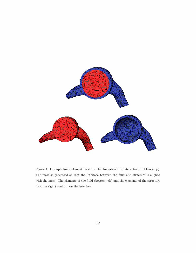
Figure 1: Example finite element mesh for the fluid-structure interaction problem (top).

The mesh is generated so that the interface between the fluid and structure is aligned

with the mesh. The elements of the fluid (bottom left) and the elements of the structure

(bottom right) conform on the interface.

12

the BDF2 scheme

xn − 4

3xn−1 +

1

3xn−2 =

2∆t

3L(xn)

is employed for the time integration. Here xn represents the value of x at the

nth time step with a fixed time step size ∆t.

The temporal discretization scheme is fully implicit, at each time step,

we obtain the solution xn = (uf , pf , xf , xs, xs) at the nth time step from the

previous two time steps by solving a sparse, nonlinear algebraic system

Fn(xn) = 0, (7)

where xn corresponds to the nodal values of the fluid velocity uf , the fluid

pressure pf , the fluid mesh displacement xf , the structure displacement xs

and the structure velocity xs at the nth time step. For simplicity, we ignore

the script n for the rest of the paper.

We note that F is a highly nonlinear function, where the nonlinearities

come from the convective term of the Navier-Stokes equations, the stabi-

lization terms and the dependency on the displacement of the moving fluid

mesh. In our fully implicit scheme, all the terms of the equations are treated

implicitly instead of explictly or semi-implicitly. This leads to a more stable

and robust scheme, but the corresponding nonlinear systems (7) are quite dif-

ficult to solve because of the different characteristics their components have.

In the fluid part of F , there are 4 unknowns per mesh point, in the moving

mesh part there are 3 unknowns per mesh point, and in the structure part

there are 6 unknowns per mesh point. The equations for the fluid is time-

dependent, nonlinear parabolic-like, the equations for the moving mesh are

elliptic type, and the equations for the structure are time dependent linear

13

hyperbolic-like. The stiffness of the system is different in the fluid part and

the structure part of the computational domain depending on the viscosity

coefficient of the flow and the wall.

3. A monolithic nonlinear solver for the coupled system of equa-

tions

In this section we introduce an overlapping domain decomposition method

for solving the coupled multi-physics system (7). The method is well studied

for each individual component of the problem, namely the incompressible

Navier-Stokes equation [25], the linear elasticity equation [28], the elliptic

moving mesh equation [7]. In a recent paper [4], it was extended to the

coupled system in two-dimensional space, here we further extend it to a full

three-dimensional problem. To design an algorithm for (7) that is highly

scalable in terms of the total compute time, many important factors need

to be taken into consideration. The basic components of the algorithm are

not new, but to arrive at the best combination, we consider not only the

properties of the nonlinear system, the properties of the domain decompo-

sition methods, but also the software and hardware of our computational

environment.

In our Newton-Krylov-Schwarz approach, the nonlinear FSI system (7)

is solved via the inexact Newton method with a cubic line search technique

[13, 14]. To obtain the new solution x(k+1) at each Newton step, the Newton

correction s(k) is approximated by solving a right-preconditioned Jacobian

system with a Krylov subspace method, GMRES [32]

JkM−1k Mks

(k) = −F(x(k)), (8)

14

where Jk is the Jacobian matrix evaluated at current solution x(k) and M−1k

is a restricted additive Schwarz preconditioner [7]. The evaluation of the

Jacobian Jk of the fully coupled system is non-trivial, especially for three-

dimensional problems. As a result, most researchers choose to approximate

the Jacobian by ignoring certain terms. The difficulty lies in the evaluation

of the cross derivatives; e.g. the derivatives of the fully coupled system with

respect to the mesh movement. One solution is to use a finite difference

approximation to calculate the cross derivatives [23], but such approxima-

tion is required at each Newton iteration and may drastically increase the

overall compute time. Another solution is to use a computationally inex-

pensive approximation of the Jacobian [20], but this may deteriorate the

overall convergence. In our implementation, we compute the Jacobian an-

alytically including all those cross derivatives. There are 66 derivatives at

some of the grid points, so the task of hand-calculating these derivatives is

time-consuming. However, this is a worthwhile excise since it saves many

Newton iterations, and can be used to provide a better preconditioner for

the Jacobian systems. We remark that, the robustness of Newton method is

often not guaranteed when the Jacobian is approximately computed.

Another critically important component of the overall solver is the precon-

ditioner, without which the iterative Jacobian solver (8) would not converge

well, and as a result, the outer inexact Newton may not converge well either.

To define the Schwarz preconditioner, we first partition the finite element

mesh Th, constructed for the initial configuration, into non-overlapping sub-

domains Ωh` , ` = 1, . . . , N , where the number of subdomains N is always the

same as the number of processors np. Then, each subdomain Ωh` is extended

15

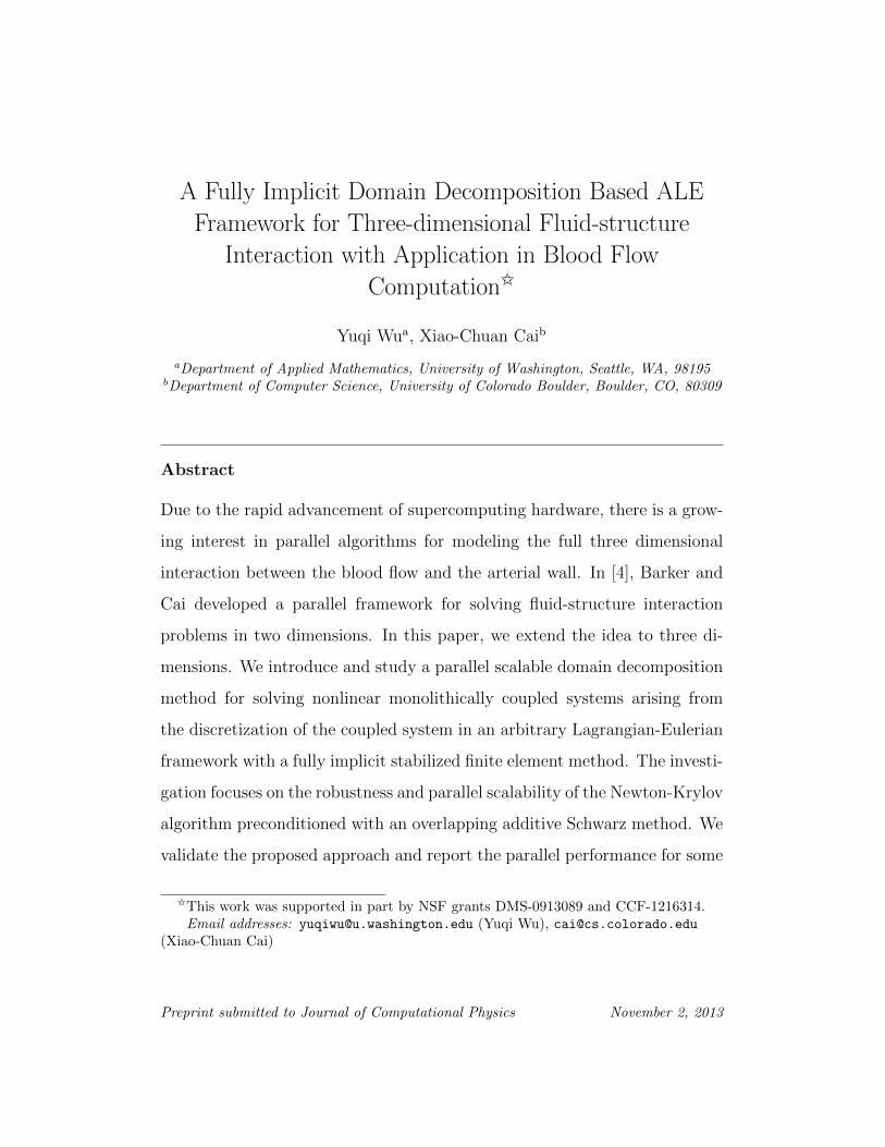
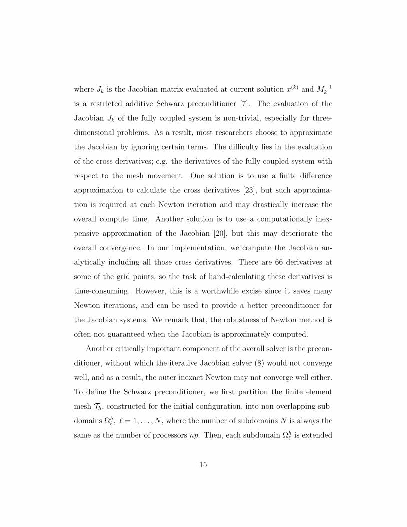
to an overlapping subdomain Ωh,δ` , where δ is an integer indicating the level

of overlap; see Figure 2 for an example. The criterions of partition inherit

from [4], where the two-dimensional meshes were studied. The partition is

element-based and the degrees of freedom defined at a mesh point is taken

into account to ensure load balancing; i.e., each subdomain has more or less

the same number of unknowns. The decomposition of the mesh is completely

independent of which physical variables are defined for a given mesh point.

A subdomain may contain both fluid and structure elements.

We define the restriction operator R` as a mapping that maps the global

vector of unknowns in Ωh to those belonging to an overlapping subdomain

Ωh,δ` . If n is the total number of unknowns in Ωh and nδ` is the number of

unknowns in Ωh,δ` , then R` is an nδ`×n sparse matrix. We construct a subdo-

main Jacobian by B` = R`JkRT` , which is a restriction of the Jacobian matrix

Jk to the subdomain Ωh,δ` . The restricted additive Schwarz preconditioner is

defined by

M−1k =

N∑`=1

(R0` )TB−1

` R`,

where R0` is the restriction to the degrees of freedom in the non-overlapping

subdomain Ωh` . In the restricted additive Schwarz preconditioner, the over-

lapping regions between the overlapping subdomains are used to provide

information to the subdomain solve, but the results of computation in the

overlapping regions are not considered in the prolongation procedure in order

to reduce the communication cost when implemented on parallel computers.

At each Newton step, the multiplication of M−1k with a vector r inside

16

the GMRES loop can be computed in the following two steps,

z` = B−1` (R`r), ` = 1, . . . , N (9)

M−1k r =

N∑`=1

(R0` )T z`. (10)

In the parallel implementation, on each processor, either a direct or an it-

erative approach can be used to solve the subdomain Jacobian systems (9).

In our application, we use a sparse LU incomplete factorization based direct

method. LU factorization can be computationally expensive if the subdo-

main problem is large, which often happens when the number of processors

is relatively small. One possible approach to improve the efficiency of LU

factorization is to control the level of fill-ins in the incomplete factoriza-

tion. There are two types of ILU factorizations. The popular point-wise

ILU works well for matrices arising from scalar partial differential equations,

but sometimes fails for coupled multi-physics problems. We choose to use a

point-block version of ILU, where we group all physical components associ-

ated with a mesh point as a block. By using the point-block version, we can

improve considerably the robustness of the subdomain preconditioner, and

at the same time improve the cache performance of the computation. The

inverse of the small point-block matrix on the diagonal of the large matrix

is computed exactly before the ILU factorization is carried out.

4. Numerical results

In this section, we report some numerical results of the proposed fully

coupled FSI solver by simulating some blood flows in three-dimensional com-

pliant arteries. We first validate the correctness of our solver by testing on a

17

Figure 2: Example partition of the domain into 4 subdomains by using ParMETIS. The

fluid elements and structure elements are marked with different colors. The top figure

shows the partition into non-overlapping subdomains, and the bottom represents a cor-

responding partition into overlapping subdomains with δ = 2. The shaded elements in

blue and green represent the corresponding fluid elements and structure elements extended

from the non-overlapping subdomains.

18

well-understood benchmark problem, then investigate the numerical behavior

and parallel performance of our solver with two complex branching geome-

tries derived from clinical data provided by colleagues at the University of

Colorado Medical School. Our solver is implemented on top of the Portable

Extensible Toolkit for Scientific computing (PETSc) library [3]. Mesh gen-

erations are carried out by CUBIT of Sandia National Laboratories [1] and

mesh partitions are obtained with ParMETIS of University of Minnesota [27].

All computations are performed on the Dell PowerEdge C6100 Cluster at the

University of Colorado Boulder.

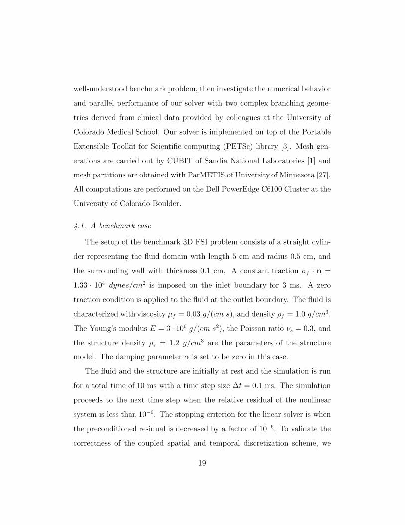
4.1. A benchmark case

The setup of the benchmark 3D FSI problem consists of a straight cylin-

der representing the fluid domain with length 5 cm and radius 0.5 cm, and

the surrounding wall with thickness 0.1 cm. A constant traction σf · n =

1.33 · 104 dynes/cm2 is imposed on the inlet boundary for 3 ms. A zero

traction condition is applied to the fluid at the outlet boundary. The fluid is

characterized with viscosity µf = 0.03 g/(cm s), and density ρf = 1.0 g/cm3.

The Young’s modulus E = 3 · 106 g/(cm s2), the Poisson ratio νs = 0.3, and

the structure density ρs = 1.2 g/cm3 are the parameters of the structure

model. The damping parameter α is set to be zero in this case.

The fluid and the structure are initially at rest and the simulation is run

for a total time of 10 ms with a time step size ∆t = 0.1 ms. The simulation

proceeds to the next time step when the relative residual of the nonlinear

system is less than 10−6. The stopping criterion for the linear solver is when

the preconditioned residual is decreased by a factor of 10−6. To validate the

correctness of the coupled spatial and temporal discretization scheme, we

19

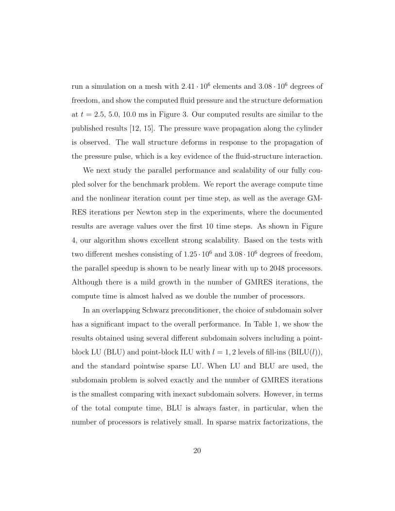
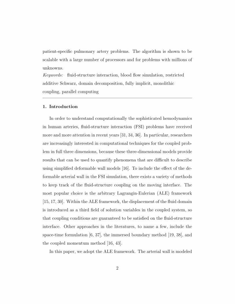
run a simulation on a mesh with 2.41 · 106 elements and 3.08 · 106 degrees of

freedom, and show the computed fluid pressure and the structure deformation

at t = 2.5, 5.0, 10.0 ms in Figure 3. Our computed results are similar to the

published results [12, 15]. The pressure wave propagation along the cylinder

is observed. The wall structure deforms in response to the propagation of

the pressure pulse, which is a key evidence of the fluid-structure interaction.

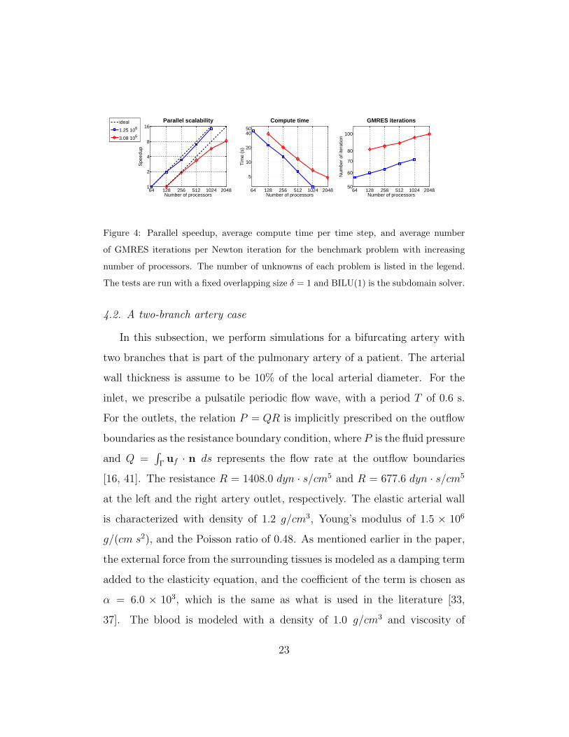
We next study the parallel performance and scalability of our fully cou-

pled solver for the benchmark problem. We report the average compute time

and the nonlinear iteration count per time step, as well as the average GM-

RES iterations per Newton step in the experiments, where the documented

results are average values over the first 10 time steps. As shown in Figure

4, our algorithm shows excellent strong scalability. Based on the tests with

two different meshes consisting of 1.25 · 106 and 3.08 · 106 degrees of freedom,

the parallel speedup is shown to be nearly linear with up to 2048 processors.

Although there is a mild growth in the number of GMRES iterations, the

compute time is almost halved as we double the number of processors.

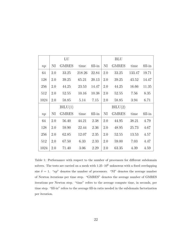
In an overlapping Schwarz preconditioner, the choice of subdomain solver

has a significant impact to the overall performance. In Table 1, we show the

results obtained using several different subdomain solvers including a point-

block LU (BLU) and point-block ILU with l = 1, 2 levels of fill-ins (BILU(l)),

and the standard pointwise sparse LU. When LU and BLU are used, the

subdomain problem is solved exactly and the number of GMRES iterations

is the smallest comparing with inexact subdomain solvers. However, in terms

of the total compute time, BLU is always faster, in particular, when the

number of processors is relatively small. In sparse matrix factorizations, the

20

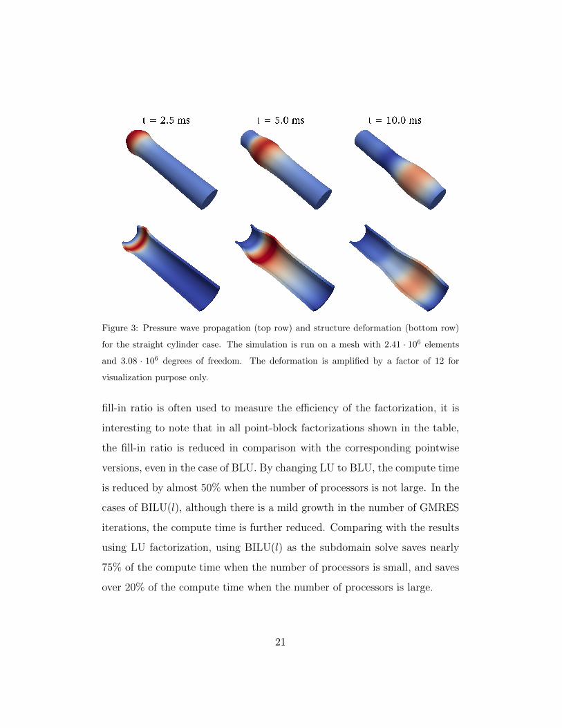
Figure 3: Pressure wave propagation (top row) and structure deformation (bottom row)

for the straight cylinder case. The simulation is run on a mesh with 2.41 · 106 elements

and 3.08 · 106 degrees of freedom. The deformation is amplified by a factor of 12 for

visualization purpose only.

fill-in ratio is often used to measure the efficiency of the factorization, it is

interesting to note that in all point-block factorizations shown in the table,

the fill-in ratio is reduced in comparison with the corresponding pointwise

versions, even in the case of BLU. By changing LU to BLU, the compute time

is reduced by almost 50% when the number of processors is not large. In the

cases of BILU(l), although there is a mild growth in the number of GMRES

iterations, the compute time is further reduced. Comparing with the results

using LU factorization, using BILU(l) as the subdomain solve saves nearly

75% of the compute time when the number of processors is small, and saves

over 20% of the compute time when the number of processors is large.

21

LU BLU

np NI GMRES time fill-in NI GMRES time fill-in

64 2.0 33.25 218.26 22.84 2.0 33.25 133.47 19.71

128 2.0 39.25 65.21 20.13 2.0 39.25 43.52 14.47

256 2.0 44.25 23.53 14.47 2.0 44.25 16.66 11.35

512 2.0 52.55 10.16 10.38 2.0 52.55 7.56 8.35

1024 2.0 58.85 5.14 7.15 2.0 58.85 3.94 6.71

BILU(1) BILU(2)

np NI GMRES time fill-in NI GMRES time fill-in

64 2.0 56.40 44.21 2.38 2.0 44.95 38.21 4.79

128 2.0 59.90 22.44 2.36 2.0 48.95 25.73 4.67

256 2.0 62.85 12.07 2.35 2.0 52.55 13.53 4.57

512 2.0 67.50 6.33 2.33 2.0 59.00 7.03 4.47

1024 2.0 71.40 3.06 2.29 2.0 63.35 4.39 4.59

Table 1: Performance with respect to the number of processors for different subdomain

solvers. The tests are carried on a mesh with 1.25 · 106 unknowns with a fixed overlapping

size δ = 1. “np” denotes the number of processors. “NI” denotes the average number

of Newton iterations per time step. “GMRES” denotes the average number of GMRES

iterations per Newton step. “time” refers to the average compute time, in seconds, per

time step. “fill-in” refers to the average fill-in ratio needed in the subdomain factorization

per iteration.

22

64 128 256 512 1024 20481

2

4

8

16Parallel scalability

Number of processors

Spe

edup

64 128 256 512 1024 2048

5

10

20

4050

Compute time

Number of processors

Tim

e (s

)

64 128 256 512 1024 204850

60

70

80

100

GMRES iterations

Number of processors

Num

ber

of it

erat

ion

ideal

1.25 106

3.08 106

Figure 4: Parallel speedup, average compute time per time step, and average number

of GMRES iterations per Newton iteration for the benchmark problem with increasing

number of processors. The number of unknowns of each problem is listed in the legend.

The tests are run with a fixed overlapping size δ = 1 and BILU(1) is the subdomain solver.

4.2. A two-branch artery case

In this subsection, we perform simulations for a bifurcating artery with

two branches that is part of the pulmonary artery of a patient. The arterial

wall thickness is assume to be 10% of the local arterial diameter. For the

inlet, we prescribe a pulsatile periodic flow wave, with a period T of 0.6 s.

For the outlets, the relation P = QR is implicitly prescribed on the outflow

boundaries as the resistance boundary condition, where P is the fluid pressure

and Q =∫

Γuf · n ds represents the flow rate at the outflow boundaries

[16, 41]. The resistance R = 1408.0 dyn · s/cm5 and R = 677.6 dyn · s/cm5

at the left and the right artery outlet, respectively. The elastic arterial wall

is characterized with density of 1.2 g/cm3, Young’s modulus of 1.5 × 106

g/(cm s2), and the Poisson ratio of 0.48. As mentioned earlier in the paper,

the external force from the surrounding tissues is modeled as a damping term

added to the elasticity equation, and the coefficient of the term is chosen as

α = 6.0 × 103, which is the same as what is used in the literature [33,

37]. The blood is modeled with a density of 1.0 g/cm3 and viscosity of

23

0.035 g/(cm s). The geometry and measured resistance values for this model

come from clinical data, provided by University of Colorado Medical School.

We initialize the Newton iteration by setting the initial wall velocity to zero

and use the solution of the steady state FSI problem as the initial conditions

for the unsteady problem. The simulations are run for 3 cardiac cycles with a

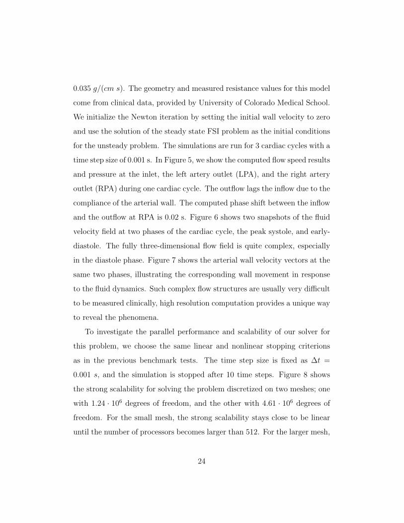
time step size of 0.001 s. In Figure 5, we show the computed flow speed results

and pressure at the inlet, the left artery outlet (LPA), and the right artery

outlet (RPA) during one cardiac cycle. The outflow lags the inflow due to the

compliance of the arterial wall. The computed phase shift between the inflow

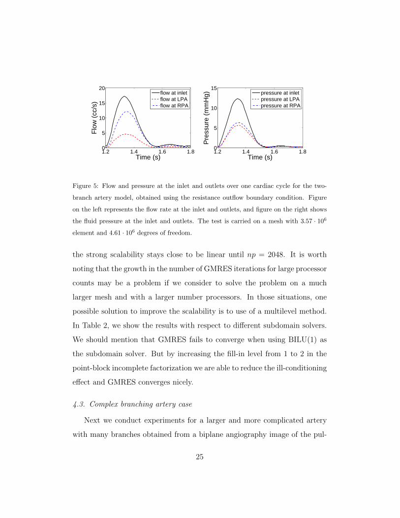
and the outflow at RPA is 0.02 s. Figure 6 shows two snapshots of the fluid

velocity field at two phases of the cardiac cycle, the peak systole, and early-

diastole. The fully three-dimensional flow field is quite complex, especially

in the diastole phase. Figure 7 shows the arterial wall velocity vectors at the

same two phases, illustrating the corresponding wall movement in response

to the fluid dynamics. Such complex flow structures are usually very difficult

to be measured clinically, high resolution computation provides a unique way

to reveal the phenomena.

To investigate the parallel performance and scalability of our solver for

this problem, we choose the same linear and nonlinear stopping criterions

as in the previous benchmark tests. The time step size is fixed as ∆t =

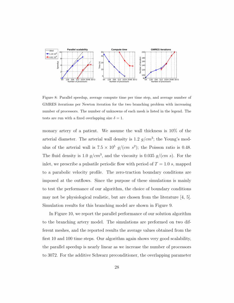
0.001 s, and the simulation is stopped after 10 time steps. Figure 8 shows

the strong scalability for solving the problem discretized on two meshes; one

with 1.24 · 106 degrees of freedom, and the other with 4.61 · 106 degrees of

freedom. For the small mesh, the strong scalability stays close to be linear

until the number of processors becomes larger than 512. For the larger mesh,

24

1.2 1.4 1.6 1.80

5

10

15

20

Time (s)

Flo

w (

cc/s

)

flow at inlet flow at LPAflow at RPA

1.2 1.4 1.6 1.80

5

10

15

Time (s)

Pre

ssur

e (m

mH

g)

pressure at inlet pressure at LPApressure at RPA

Figure 5: Flow and pressure at the inlet and outlets over one cardiac cycle for the two-

branch artery model, obtained using the resistance outflow boundary condition. Figure

on the left represents the flow rate at the inlet and outlets, and figure on the right shows

the fluid pressure at the inlet and outlets. The test is carried on a mesh with 3.57 · 106

element and 4.61 · 106 degrees of freedom.

the strong scalability stays close to be linear until np = 2048. It is worth

noting that the growth in the number of GMRES iterations for large processor

counts may be a problem if we consider to solve the problem on a much

larger mesh and with a larger number processors. In those situations, one

possible solution to improve the scalability is to use of a multilevel method.

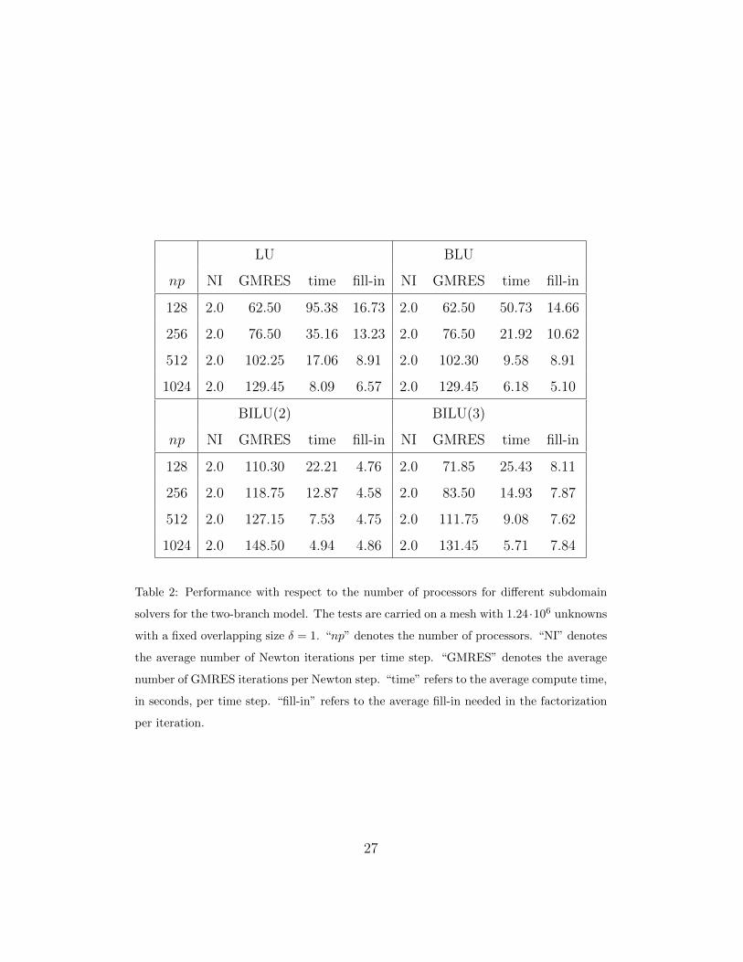
In Table 2, we show the results with respect to different subdomain solvers.

We should mention that GMRES fails to converge when using BILU(1) as

the subdomain solver. But by increasing the fill-in level from 1 to 2 in the

point-block incomplete factorization we are able to reduce the ill-conditioning

effect and GMRES converges nicely.

4.3. Complex branching artery case

Next we conduct experiments for a larger and more complicated artery

with many branches obtained from a biplane angiography image of the pul-

25

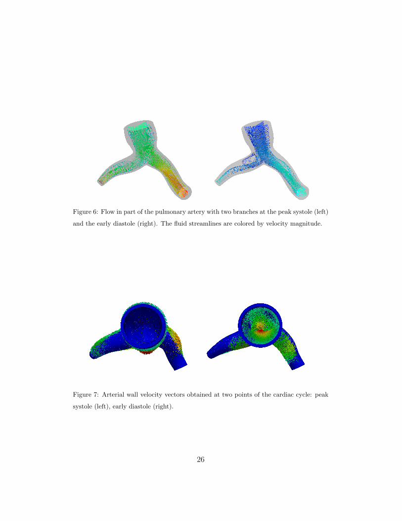
Figure 6: Flow in part of the pulmonary artery with two branches at the peak systole (left)

and the early diastole (right). The fluid streamlines are colored by velocity magnitude.

Figure 7: Arterial wall velocity vectors obtained at two points of the cardiac cycle: peak

systole (left), early diastole (right).

26

LU BLU

np NI GMRES time fill-in NI GMRES time fill-in

128 2.0 62.50 95.38 16.73 2.0 62.50 50.73 14.66

256 2.0 76.50 35.16 13.23 2.0 76.50 21.92 10.62

512 2.0 102.25 17.06 8.91 2.0 102.30 9.58 8.91

1024 2.0 129.45 8.09 6.57 2.0 129.45 6.18 5.10

BILU(2) BILU(3)

np NI GMRES time fill-in NI GMRES time fill-in

128 2.0 110.30 22.21 4.76 2.0 71.85 25.43 8.11

256 2.0 118.75 12.87 4.58 2.0 83.50 14.93 7.87

512 2.0 127.15 7.53 4.75 2.0 111.75 9.08 7.62

1024 2.0 148.50 4.94 4.86 2.0 131.45 5.71 7.84

Table 2: Performance with respect to the number of processors for different subdomain

solvers for the two-branch model. The tests are carried on a mesh with 1.24 ·106 unknowns

with a fixed overlapping size δ = 1. “np” denotes the number of processors. “NI” denotes

the average number of Newton iterations per time step. “GMRES” denotes the average

number of GMRES iterations per Newton step. “time” refers to the average compute time,

in seconds, per time step. “fill-in” refers to the average fill-in needed in the factorization

per iteration.

27

64 128 256 512 1024 2048 30721

2

4

8

16Parallel scalability

Number of processors

Spe

edup

64 128 256 512 1024 2048 3072

5

10

20

40

60Compute time

Number of processors

Tim

e (s

)

64 128 256 512 1024 2048 307290

100

120

140

160

180

220GMRES iterations

Number of processors

Num

ber

of it

erat

ion

ideal

1.24 106

4.61 106

Figure 8: Parallel speedup, average compute time per time step, and average number of

GMRES iterations per Newton iteration for the two branching problem with increasing

number of processors. The number of unknowns of each mesh is listed in the legend. The

tests are run with a fixed overlapping size δ = 1.

monary artery of a patient. We assume the wall thickness is 10% of the

arterial diameter. The arterial wall density is 1.2 g/cm3; the Young’s mod-

ulus of the arterial wall is 7.5 × 105 g/(cm s2); the Poisson ratio is 0.48.

The fluid density is 1.0 g/cm3, and the viscosity is 0.035 g/(cm s). For the

inlet, we prescribe a pulsatile periodic flow with period of T = 1.0 s, mapped

to a parabolic velocity profile. The zero-traction boundary conditions are

imposed at the outflows. Since the purpose of these simulations is mainly

to test the performance of our algorithm, the choice of boundary conditions

may not be physiological realistic, but are chosen from the literature [4, 5].

Simulation results for this branching model are shown in Figure 9.

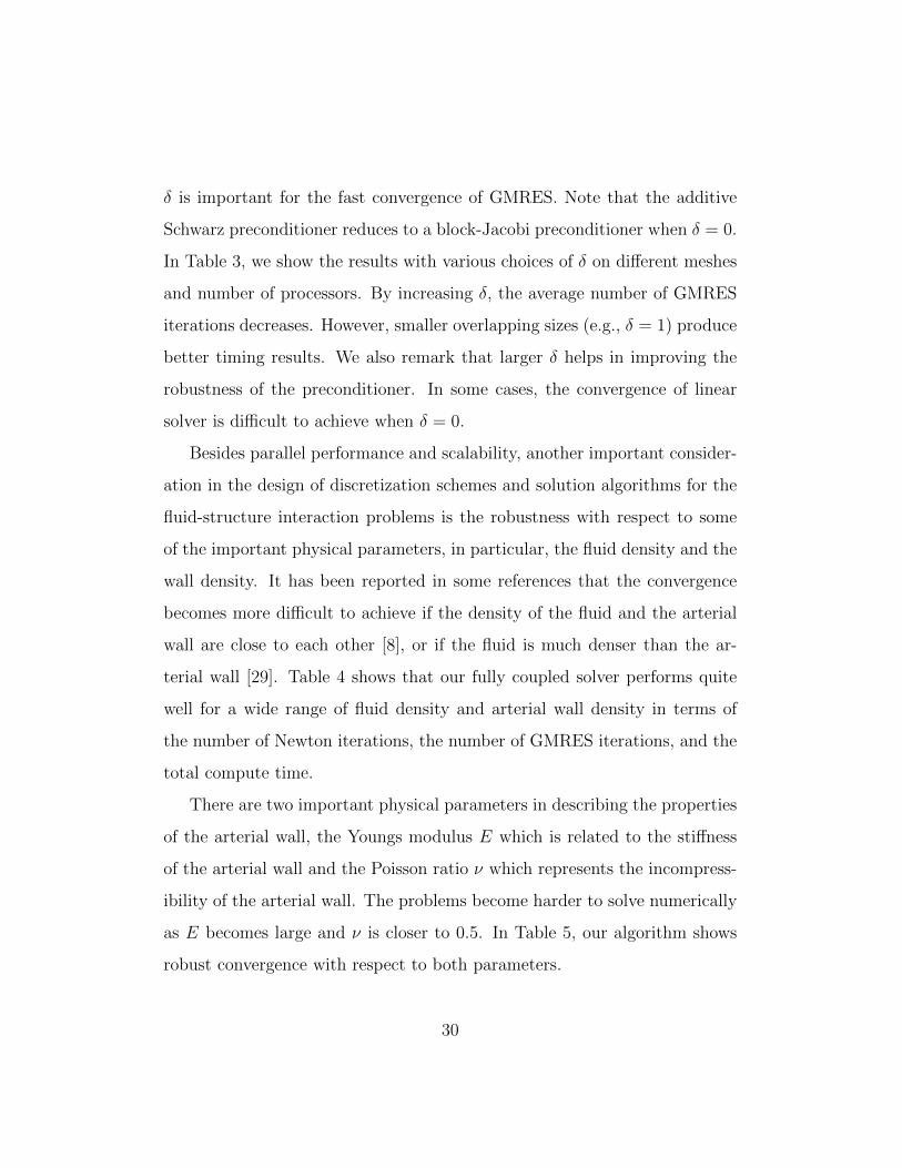
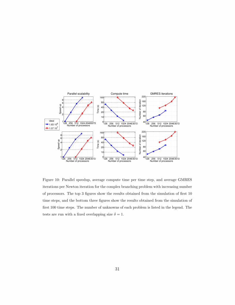
In Figure 10, we report the parallel performance of our solution algorithm

to the branching artery model. The simulations are preformed on two dif-

ferent meshes, and the reported results the average values obtained from the

first 10 and 100 time steps. Our algorithm again shows very good scalability,

the parallel speedup is nearly linear as we increase the number of processors

to 3072. For the additive Schwarz preconditioner, the overlapping parameter

28

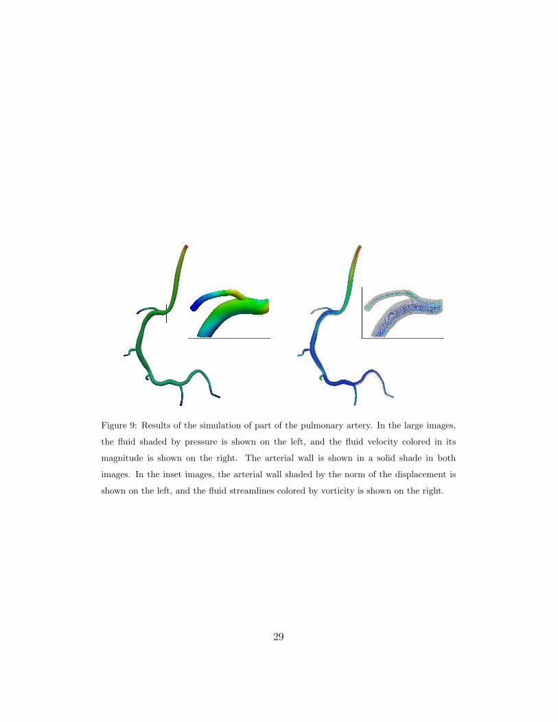
Figure 9: Results of the simulation of part of the pulmonary artery. In the large images,

the fluid shaded by pressure is shown on the left, and the fluid velocity colored in its

magnitude is shown on the right. The arterial wall is shown in a solid shade in both

images. In the inset images, the arterial wall shaded by the norm of the displacement is

shown on the left, and the fluid streamlines colored by vorticity is shown on the right.

29

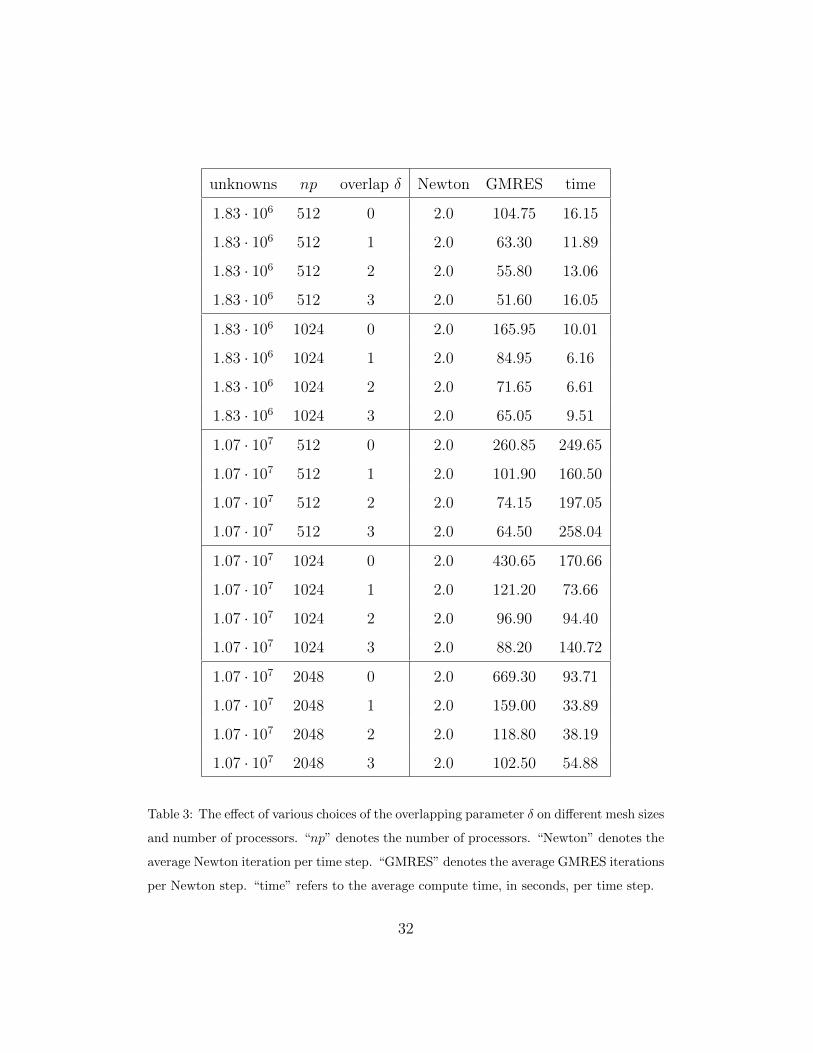
δ is important for the fast convergence of GMRES. Note that the additive

Schwarz preconditioner reduces to a block-Jacobi preconditioner when δ = 0.

In Table 3, we show the results with various choices of δ on different meshes

and number of processors. By increasing δ, the average number of GMRES

iterations decreases. However, smaller overlapping sizes (e.g., δ = 1) produce

better timing results. We also remark that larger δ helps in improving the

robustness of the preconditioner. In some cases, the convergence of linear

solver is difficult to achieve when δ = 0.

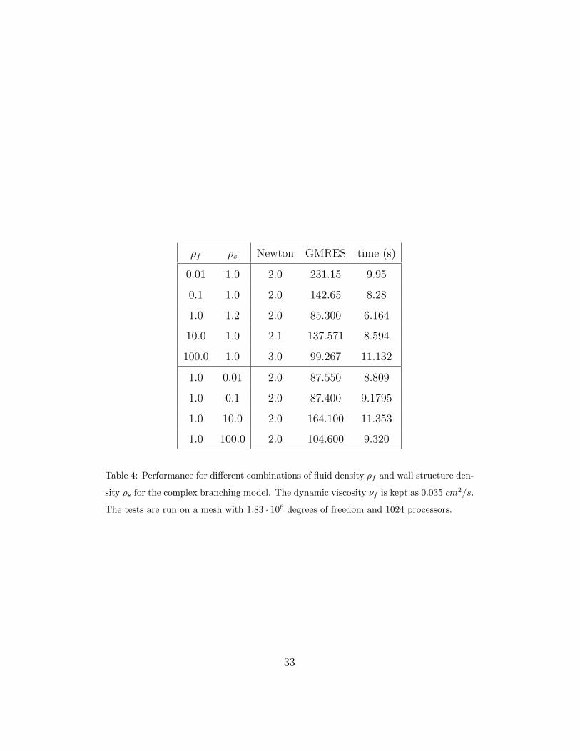
Besides parallel performance and scalability, another important consider-

ation in the design of discretization schemes and solution algorithms for the

fluid-structure interaction problems is the robustness with respect to some

of the important physical parameters, in particular, the fluid density and the

wall density. It has been reported in some references that the convergence

becomes more difficult to achieve if the density of the fluid and the arterial

wall are close to each other [8], or if the fluid is much denser than the ar-

terial wall [29]. Table 4 shows that our fully coupled solver performs quite

well for a wide range of fluid density and arterial wall density in terms of

the number of Newton iterations, the number of GMRES iterations, and the

total compute time.

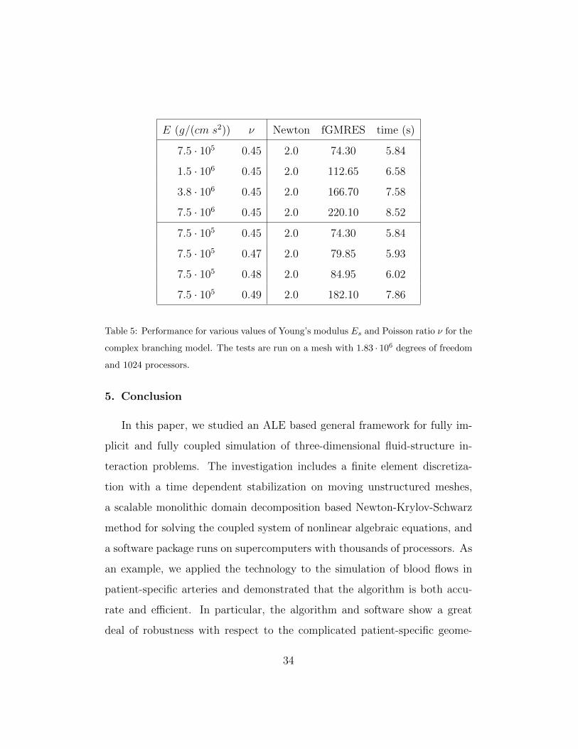
There are two important physical parameters in describing the properties

of the arterial wall, the Youngs modulus E which is related to the stiffness

of the arterial wall and the Poisson ratio ν which represents the incompress-

ibility of the arterial wall. The problems become harder to solve numerically

as E becomes large and ν is closer to 0.5. In Table 5, our algorithm shows

robust convergence with respect to both parameters.

30

128 256 512 1024 204830721

2

4

6

8

Number of processors

Sp

ee

d u

p

128 256 512 1024 204830725

10

20

40

80

160

Number of processors

Tim

e (

s)

Compute time

128 256 512 1024 204830725

10

20

40

80

160

Number of processors

Tim

e (

s)

128 256 512 1024 2048307240

60

80

120

160

220

Number of processors

Nu

mb

er

of

ite

ratio

n

GMRES iterations

128 256 512 1024 2048307240

60

80

120

160

220

Number of processors

Nu

mb

er

of

ite

ratio

n

128 256 512 1024 204830721

2

4

6

8

Number of processors

Sp

ee

d u

p

Parallel scalability

ideal

1.83 106

1.07 107

Figure 10: Parallel speedup, average compute time per time step, and average GMRES

iterations per Newton iteration for the complex branching problem with increasing number

of processors. The top 3 figures show the results obtained from the simulation of first 10

time steps, and the bottom three figures show the results obtained from the simulation of

first 100 time steps. The number of unknowns of each problem is listed in the legend. The

tests are run with a fixed overlapping size δ = 1.

31

unknowns np overlap δ Newton GMRES time

1.83 · 106 512 0 2.0 104.75 16.15

1.83 · 106 512 1 2.0 63.30 11.89

1.83 · 106 512 2 2.0 55.80 13.06

1.83 · 106 512 3 2.0 51.60 16.05

1.83 · 106 1024 0 2.0 165.95 10.01

1.83 · 106 1024 1 2.0 84.95 6.16

1.83 · 106 1024 2 2.0 71.65 6.61

1.83 · 106 1024 3 2.0 65.05 9.51

1.07 · 107 512 0 2.0 260.85 249.65

1.07 · 107 512 1 2.0 101.90 160.50

1.07 · 107 512 2 2.0 74.15 197.05

1.07 · 107 512 3 2.0 64.50 258.04

1.07 · 107 1024 0 2.0 430.65 170.66

1.07 · 107 1024 1 2.0 121.20 73.66

1.07 · 107 1024 2 2.0 96.90 94.40

1.07 · 107 1024 3 2.0 88.20 140.72

1.07 · 107 2048 0 2.0 669.30 93.71

1.07 · 107 2048 1 2.0 159.00 33.89

1.07 · 107 2048 2 2.0 118.80 38.19

1.07 · 107 2048 3 2.0 102.50 54.88

Table 3: The effect of various choices of the overlapping parameter δ on different mesh sizes

and number of processors. “np” denotes the number of processors. “Newton” denotes the

average Newton iteration per time step. “GMRES” denotes the average GMRES iterations

per Newton step. “time” refers to the average compute time, in seconds, per time step.

32

ρf ρs Newton GMRES time (s)

0.01 1.0 2.0 231.15 9.95

0.1 1.0 2.0 142.65 8.28

1.0 1.2 2.0 85.300 6.164

10.0 1.0 2.1 137.571 8.594

100.0 1.0 3.0 99.267 11.132

1.0 0.01 2.0 87.550 8.809

1.0 0.1 2.0 87.400 9.1795

1.0 10.0 2.0 164.100 11.353

1.0 100.0 2.0 104.600 9.320

Table 4: Performance for different combinations of fluid density ρf and wall structure den-

sity ρs for the complex branching model. The dynamic viscosity νf is kept as 0.035 cm2/s.

The tests are run on a mesh with 1.83 · 106 degrees of freedom and 1024 processors.

33

E (g/(cm s2)) ν Newton fGMRES time (s)

7.5 · 105 0.45 2.0 74.30 5.84

1.5 · 106 0.45 2.0 112.65 6.58

3.8 · 106 0.45 2.0 166.70 7.58

7.5 · 106 0.45 2.0 220.10 8.52

7.5 · 105 0.45 2.0 74.30 5.84

7.5 · 105 0.47 2.0 79.85 5.93

7.5 · 105 0.48 2.0 84.95 6.02

7.5 · 105 0.49 2.0 182.10 7.86

Table 5: Performance for various values of Young’s modulus Es and Poisson ratio ν for the

complex branching model. The tests are run on a mesh with 1.83 · 106 degrees of freedom

and 1024 processors.

5. Conclusion

In this paper, we studied an ALE based general framework for fully im-

plicit and fully coupled simulation of three-dimensional fluid-structure in-

teraction problems. The investigation includes a finite element discretiza-

tion with a time dependent stabilization on moving unstructured meshes,

a scalable monolithic domain decomposition based Newton-Krylov-Schwarz

method for solving the coupled system of nonlinear algebraic equations, and

a software package runs on supercomputers with thousands of processors. As

an example, we applied the technology to the simulation of blood flows in

patient-specific arteries and demonstrated that the algorithm is both accu-

rate and efficient. In particular, the algorithm and software show a great

deal of robustness with respect to the complicated patient-specific geome-

34

tries, large meshes and large number of processors. Superlinear scalability

was observed for problems with tens of millions of degrees of freedom and

on a machine with more than three thousand processors. We plan to further

extend the approach and the software framework to include multilevel capa-

bility, which is needed for supercomputer with larger processor counts and

for large-scale simulations.

6. Acknowledgments

Special thanks to Professor Kendall Hunter and Professor Robin Shandas

for their helpful discussions and acquiring clinical data for our model. Thanks

also to the PETSc team of Argonne National Laboratory for their help and

technical support on using the PETSc library.

References

[1] The CUBIT Geometry and Mesh Generation Toolkit, Sandia National

Laboratories, 2012. Http://cubit.sandia.gov/.

[2] S. Badia, A. Quaini, A. Quarteroni, Modular vs. non-modular precondi-

tioners for fluid-structure systems with large added-mass effect, Comput.

Methods Appl. Mech. Engrg. 197 (2008) 4216–4232.

[3] S. Balay, J. Brown, K. Buschelman, V. Eijkhout, W.D. Gropp,

D. Kaushik, M.G. Knepley, L. McInnes, B. Smith, H. Zhang, PETSc

User Manual, Technical Report, Argonne National Laboratory, 2011.

35

[4] A.T. Barker, X.-C. Cai, Scalable parallel methods for monolithic cou-

pling in fluid-structure interaction with application to blood flow mod-

eling, J. Comput. Phys. 229 (2010) 642–659.

[5] A.T. Barker, X.-C. Cai, Two-level Newton and hybrid Schwarz precon-

ditioners for fluid-structure interation, SIAM J. Sci. Comput. 32 (2010)

2395–2417.

[6] Y. Bazilevs, V.M. Calo, T.J.R. Hughes, Y. Zhang, Isogeometric fluid-

structure interaction: theory, algorithms, and computations, Comput.

Mech. 43 (2008) 3–37.

[7] X.-C. Cai, M. Sarkis, A restricted additive Schwarz preconditioner for

general sparse linear systems, SIAM J. Sci. Comput. 21 (1999) 792–797.

[8] P. Causin, J.F. Gerbeau, F. Nobile, Added-mass effect in the design of

partitioned algorithms for fluid-structure problems, Comput. Methods

Appl. Mech. Engrg. 194 (2005) 4506–4627.

[9] P. Crosetto, S. Deparis, G. Fourestey, A. Quarteroni, Parallel algorithm

for fluid-structure interaction problems in haemodynamics, SIAM J. Sci.

Comput. 33 (2011) 1598–1622.

[10] P. Crosetto, P. Raymond, S. Deparis, D. Kontaxakis, N. Stergiopulos,

A. Quarteroni, Fluid structure interaction simulations of physiological

blood flow in the aorta, Computers and Fluids 43 (2011) 46–57.

[11] J. Dennis, R. Schnabel, Numerical Methods for Unconstrained Optima-

tization and Nonlinear Equations, SIAM, Philadelphia, 1996.

36

[12] S. Deparis, M. Discacciati, G. Fourestey, A. Quarteroni, Fluid-structure

algorithms based on Steklov-Poincare operators, Comput. Methods

Appl. Mech. Engrg. 195 (2006) 5797–5812.

[13] S.C. Eisenstat, H.F. Walker, Globally convergent inexact Newton

method, SIAM J. Optim. 4 (1994) 393–422.

[14] S.C. Eisenstat, H.F. Walker, Choosing the forcing terms in an inexact

Newton method, SIAM J. Sci. Comput. 17 (1996) 16–32.

[15] M.A. Fernandez, M. Moubachir, A Newton method using exact Jaco-

bians for solving fluid-structure coupling, Comput. Struct. 83 (2005)

127–142.

[16] C.A. Figueroa, I.E. Vignon-Clementel, K.E. Jansen, T.J.R. Hughes,

C.A. Taylor, A coupled momentum method for modeling blood flow in

three-dimensional deformable arteries, Comput. Methods Mech. Engrg.

195 (2006) 5685–5706.

[17] L. Formaggia, J.F. Gerbeau, F. Nobile, A. Quarteroni, On the coupling

of 3D and 1D Navier-Stokes equations for flow problems in compliant

vessels, Comput. Methods Appl. Mech. Engrg. 191 (2001) 561–582.

[18] L. Formaggia, A. Quarteroni, A. Veneziani (Eds.), Cardiovascular Math-

ematics: Modeling and Simulation of the Circulatory System, Springer,

Milan, 2009.

[19] L. Ge, F. Sotiropoulos, A numerical method for solving 3D unsteady in-

compressible Navier-Stokes equations in curvilinear domains with com-

plex immersed boundaries, J. Comput. Phys. 225 (2007) 1782–1809.

37

[20] J.F. Gerbeau, M. Vidrascu, A quasi-Newton algorithm based on a re-

duced model for fluid structure problems in blood flows, ESAIM - Math.

Model. Numer. Anal. 37 (2003) 631–647.

[21] L. Grinberg, G.E. Karniadakis, A scalable domain decomposition

method for ultra-parallel arterial flow simulations, Commun. Comput.

Phys. 4 (2008) 1151–1169.

[22] D.F. Hawken, J.J. Gottlieb, J.S. Hansen, Review of some adaptive node-

movement techniques in finite-element and finite-difference solutions of

partial differential equations, J. Comput. Phys. 95 (1991) 254–302.

[23] M. Heil, An efficient solver for the fully coupled solution of large-

displacement fluid-structure interaction problems, Comput. Methods

Appl. Mech. Engrg. 193 (2004) 1–23.

[24] J.J. Heys, T.A. Manteuffel, S.F. McCormick, J.W. Ruge, First-order sys-

tem least squares (FOSLS) for coupled fluid-elastic problems, J. Com-

put. Phys. 195 (2004) 560–575.

[25] F.-N. Hwang, X.-C. Cai, Parallel fully coupled Schwarz preconditioners

for saddle-point problems, Electron. Trans. Numer. Anal. 22 (2006) 146–

162.

[26] A.A. Johnson, T.E. Tezduyar, Mesh update strategies in parallel finite

element computations of flow problems with moving boundaries and

interfaces, Comput. Methods Appl. Mech. Engrg. 119 (1994) 73–94.

[27] G. Karypis, METIS/ParMETIS web page, University of Minnesota,

2012. Http://glaros.dtc.umn.edu/gkhome/views/metis.

38

[28] A. Klawonn, L.F. Pavarino, Overlapping Schwarz methods for mixed

linear elasticity and Stokes problems, Comput. Methods Appl. Mech.

Engrg. 165 (1998) 233–245.

[29] C. Michler, E.H. van Brunmmelen, R. de Borst, The relevance of conser-

vation for stability and accuracy of numerical methods for fluid-structure

interactions, Comput. Methods Appl. Mech. Engrg. 192 (2003) 4195–

4215.

[30] F. Nobile, Numerical Approximation of Fluid-structure Interatction

Problems with Application to Haemodynamics, Ph.D. thesis, Ecole

Polytechnique Federale de Lausanne, Lausanne, Switzerland, 2001.

[31] A. Quarteroni, M. Tuveri, A. Veneziani, Computational vascular fluid

dynamics: problems, models and methods, Comput. Visual. Sci. 2 (2000)

163–197.

[32] Y. Saad, M.H. Schultz, GMRES: A generalized minimal residual algo-

rithm for solving nonsymmetric linear system, SIAM J. Sci. Stat. Comp.

7 (1986) 856–869.

[33] K. Takizawa, J. Christopher, T.E. Tezduyar, S. Sathe, Space-time finite

element computation of arterial fluid-structure interactions with patient-

specific data, Int. J. Numer. Meth. Biomed. Engrg. 26 (2010) 101–116.

[34] C.A. Taylor, M.T. Draney, Experimental and computational methods in

cardiovascular fluid mechanics, Ann. Rev. Fluid Mech. 36 (2004) 197–

231.

39

[35] C.A. Taylor, T.J.R. Hughes, C.K. Zarins, Finite element modeling of

blood flow in arteries, Comput. Methods Mech. Engrg. 158 (1998) 155–

196.

[36] C.A. Taylor, J.D. Humphrey, Open problems in computational vascu-

lar biomechanics: Hemodynamics and arterial wall mechanics, Comput.

Methods Appl. Mech. Engrg. 198 (2009) 3514–3523.

[37] T.E. Tezduyar, S. Sathe, T. Cragin, B. Nanna, B.S. Conklin, J. Pause-

wang, M. Schwaab, Modelling of fluid-structure interactions with the

space-time finite elements: Arterial fluid mechanics, Int. J. Numer.

Meth. Fluids 54 (2007) 901–922.

[38] H. Wang, J. Chessa, W.K. Liu, T. Belytschko, The immersed/fictitious

element method for fluid-structure interaction: volumetric consistency,

compressibility and thin members, Int. J. Numer. Meth. Engng. 74

(2008) 32–55.

[39] C.H. Whiting, Stabilized Finite Element Methods for Fluid Dynamics

Using a Hierarchical Basis, Ph.D. thesis, Rensselaer Polytechnic Insti-

tute, Troy, New York, 1999.

[40] C.H. Whiting, K.E. Jansen, A stabilized finite element method for the

incompressible Navier-Stokes equations using a hierarchical basis, Int.

J. Numer. Meth. Fluids 35 (2001) 93–116.

[41] Y. Wu, X.-C. Cai, A parallel two-level method for simulating blood flows

in branching arteries with the resistive boundary condition, Computers

and Fluids 45 (2011) 92–102.

40

[42] C. Yang, J. Cao, X.-C. Cai, A fully implicit domain decomposition al-

gorithm for shallow water equations on the cubed-sphere, SIAM J. Sci.

Comput. 32 (2010) 418–438.

[43] M. Zhou, O. Sahni, H.J. Kim, C.A. Figueroa, C.A. Taylor, M.S. Shep-

hard, K.E. Jansen, Cardiovascular flow simulation at extreme scale,

Comput. Mech. 46 (2010) 71–82.

41