A fully polynomial approximation scheme for the single machine weighted total tardiness problem with a common due date

Theoretical Computer Science 369 (2006) 230–238www.elsevier.com/locate/tcs

A fully polynomial approximation scheme for the single machineweighted total tardiness problem with a common due date

Hans Kellerera, Vitaly A. Strusevichb,∗aInstitut für Statistik und Operations Research, Universität Graz, UniversitätsstraYe 15, A-8010, Graz, Austria

bSchool of Computing and Mathematical Sciences, University of Greenwich, Old Royal Naval College, Park Row, Greenwich,London SE10 9LS, UK

Received 26 January 2006; received in revised form 16 August 2006; accepted 25 August 2006

Communicated by Ding-Zhu Du

Abstract

We develop a fully polynomial-time approximation scheme (FPTAS) for minimizing the weighted total tardiness on a singlemachine, provided that all due dates are equal. The FPTAS is obtained by converting an especially designed pseudopolynomialdynamic programming algorithm.© 2006 Elsevier B.V. All rights reserved.

Keywords: Single machine scheduling; Weighted total tardiness; Dynamic programming; FPTAS

1. Introduction

In this paper we consider a single machine scheduling problem of minimizing total weighted tardiness about acommon due date.

The jobs of set N = {1, 2, . . . , n} have to be processed without preemption on a single machine. The processingof job j ∈ N takes pj time units. There is a positive weight wj associated with job j , which indicates its relativeimportance. The completion time of job j ∈ N in a feasible schedule S is denoted by Cj (S), or shortly Cj if it is clearwhich schedule is referred to. It is desired to complete job j by a given due date dj .

A job j is said to be early if Cj − dj �0, and late if Cj − dj > 0; in the latter case its tardiness is defined asTj = Cj − dj . The aim is to find a schedule that minimizes the function

∑j∈N wjTj . This problem is traditionally

denoted by 1‖∑wjTj .Problem 1‖∑wjTj is NP-hard in the strong sense if the weights are not all equal (see [8,11]) and is solvable in

pseudopolynomial time for a fixed number of distinct due dates (see [7]). If the weights are equal, problem 1‖∑ Tj

is NP-hard in the ordinary sense as proved by Du and Leung [5] and is solvable by a pseudopolynomial dynamicprogramming (DP) algorithm developed by Lawler [8].

∗ Corresponding author. Tel.: +44 20 8331 8662; fax: +44 20 8331 8665.E-mail addresses: [email protected] (H. Kellerer), [email protected] (V.A. Strusevich).

0304-3975/$ - see front matter © 2006 Elsevier B.V. All rights reserved.doi:10.1016/j.tcs.2006.08.030

http://www.elsevier.com/locate/tcs

mailto:[email protected]

mailto:[email protected]

H. Kellerer, V.A. Strusevich / Theoretical Computer Science 369 (2006) 230–238 231

In this paper we focus on the situation that the due date is common for all jobs, i.e., dj = d, j ∈ N . We are onlyinterested in the case that the sum of all processing times exceeds the due date d. The resulting problem is denoted by1|dj = d|∑wjTj . It is proved to be NP-hard in the ordinary sense by Yuan [15]. For this problem, Lawler and Moore[10] provide a pseudopolynomial DP algorithm that requires O(n2d) time and demonstrate that the problem with equalweights is solvable in O(n2) time.

Various aspects of solving the general problem 1‖∑wjTj and its variants have attracted considerable attention, seesurveys [1,13]. The problem traditionally plays the role of a testing ground for verifying scheduling techniques; see,e.g., the influential papers [3,12].

Since the main topic of this paper is that of analysis of approximation algorithms, we recall some relevant definitions.For a scheduling problem of minimizing a function Z(S) a polynomial-time algorithm that finds a feasible solutionSH such that Z(SH ) is at most ��1 times the optimal value Z(S∗) is called a �-approximation algorithm; the valueof � is called a worst-case ratio bound. If a problem admits a �-approximation algorithm it is said to be approximablewithin a factor �. A family of �-approximation algorithms is called a fully polynomial-time approximation scheme, oran FPTAS, if � = 1 + � for any � > 0 and the running time is polynomial with respect to both the length of the probleminput and 1/�. Notice that a problem that is NP-hard in the strong sense admits no FPTAS unless P = NP .

For problem 1‖∑ Tj , Lawler [9] converts his DP algorithm into an FPTAS that requires O(n7/�) time. Della Croceet al. [4] examine several popular constructive and decomposition heuristics for problem 1‖∑ Tj , and demonstratethat none of them guarantees a constant worst-case ratio.

For problem 1‖∑wjTj with arbitrary weights Cheng et al. [2] give an (n−1)-approximation algorithm that requiresO(n2) time. For the common due date problem 1|dj = d |∑wjTj , Fathi and Nuttle [6] provide a 2-approximationalgorithm that requires O(n2) time. Kolliopoulos and Steiner [7] give an approximation scheme for the problem witha fixed number of distinct due dates, however, the running time of their algorithm is pseudopolynomial since it isbounded by a polynomial of the largest weight. This leaves an open question regarding the existence of an FPTASfor the problem with a fixed number of distinct due dates. In this paper we give the positive answer to this question,provided that all due dates are equal.

The remainder of this paper is organized as follows. In Section 2 we describe a DP algorithm for problem 1|dj =d |∑wjTj , and then in Section 3 we convert it into an FPTAS. Concluding remarks are given in Section 4.

2. Dynamic programming

In this section we present a DP algorithm for problem 1|dj = d|∑wjTj . Although the problem is known to besolvable by DP, see [10,7], for our purposes we need an algorithm of a special structure that allows us to convert it intoan FPTAS.

Throughout this paper, we assume that in problem 1|dj = d|∑wjTj the jobs are numbered in such a way that

p1

w1� p2

w2� · · · � pn

wn

. (1)

We call the sequence of jobs numbered in accordance with (1) a Smith sequence or a WSPT sequence (weightedshortest processing time). Recall that in an optimal schedule for the classical single machine problem of minimizingthe weighted sum of the completion times, the jobs are processed according to the WSPT sequence, see [14].

For problem 1|dj = d|∑wjTj , an optimal schedule belongs to the class of schedules in which the early jobs areprocessed starting at time zero and are followed by the straddling job that starts before time d and is completed noearlier than time d; in turn, the straddling job is followed by the block of late jobs. The early jobs can be processed inany order, while the late jobs that start at or after the due date are processed according to their numbering given by (1).For convenience, we further assume that the early jobs are also scheduled in the order of their numbering.

Suppose that a certain job is chosen as the straddling job. Renumber the remaining jobs taken according to the WSPTrule by the integers 1, 2, . . . , m, where m = n − 1.

A feasible schedule for problem 1|dj = d|∑wjTj with a fixed straddling job can be found by inserting the straddlingjob into a schedule for processing the jobs 1, 2, . . . , m in such a way that:

(i) all early jobs are sequenced in the order of their numbering and are processed as a block without intermediateidle time, starting at time zero, and completed by the due date;

232 H. Kellerer, V.A. Strusevich / Theoretical Computer Science 369 (2006) 230–238

(ii) all late jobs are sequenced in the order of their numbering and are processed as a block without intermediate idletime, starting at the due date.

Having chosen the straddling job, introduce an auxiliary problem of finding a schedule that satisfies the conditions(i) and (ii) above and minimizes the total weighted tardiness of the remaining jobs 1, 2, . . . , m. We call this problemthe stop due date problem and denote it by 1|(p, w), dj = dstop|∑wjTj , provided that the processing time and theweight of the chosen straddling job are equal to p and w, respectively.

Let us introduce the following schedules:S∗—an optimal schedule for the original problem 1|dj = d|∑wjTj of processing n jobs;

Sm—a feasible schedule for the problem 1|(p, w), dj = dstop|∑wjTj of processing m = n − 1 jobs;S(p, w)—a feasible schedule for the original problem 1|dj = d|∑wjTj of processing n jobs with a fixed straddlingjob with the processing time p and weight w;S∗(p, w)—the best schedule for problem 1|dj = d|∑wjTj with a fixed straddling job with the processing time pand weight w;S∗

m—be a schedule that is feasible for problem 1|(p, w), dj = dstop|∑wjTj such that after inserting the straddlingjob with the processing time p and weight w, schedule S∗(p, w) is obtained.

For a chosen straddling job with the processing time p and weight w, we formulate the stop due date problem1|(p, w), dj = dstop|∑wjTj as a quadratic knapsack problem and present a DP algorithm for its solution.

Introduce the following Boolean decision variables

xj ={

1 if job j completes after the due date d,

0 otherwise.

The total weighted tardiness for a schedule Sm that is feasible for problem 1|(p, w), dj = dstop|∑wjTj is given by

Zm =m∑

j=1wj

(j∑

i=1pixi

)xj = ∑

1� i � j �m

piwjxixj ,

where

m∑j=1

pj (1 − xj )�d, xj ∈ {0, 1}, j = 1, 2, . . . , m.

The case that p�d −∑mj=1 pj (1−xj ) can be ignored, since in this case the chosen job effectively is not straddling,

i.e., there exists a better schedule for the original problem 1|dj = d|∑wjTj with another straddling job.Given the values of xj ∈ {0, 1}, j = 1, 2, . . . , m, we can create the corresponding schedule Sm feasible for problem

1|(p, w), dj = dstop|∑wjTj by scheduling the jobs with xj = 0 as the block of early jobs and the jobs with xj = 1as the block of late jobs; the jobs of each block are sequenced in the order of their numbering.

Finding the required values of xj , j = 1, 2, . . . , m, can be done by the following DP algorithm. The jobs are scannedin the order of their numbering. A typical state after the values x1, x2, . . . , xk have been assigned is represented by astate of the form

(k, Zk, yk, Wk),

where, k is the number of the assigned jobs; Zk is the current value of the objective function; yk := ∑kj=1 pjxj ,

the total processing time of late jobs, and

Wk :=k∑

j=1wjxj

denotes the total weight of the jobs 1, . . . , k processed after the due date.Assume that the values Ak = ∑k

j=1 pj are computed in advance for all k, k = 1, . . . , m. The algorithm starts with thestate (0, 0, 0, 0). In iteration k of the algorithm a move from a state (k, Zk, yk, Wk) to a state (k +1, Zk+1, yk+1, Wk+1)

is done as follows:


If job k + 1 is scheduled early, i.e., xk+1 = 0, then

Zk+1 = Zk, yk+1 = yk, Wk+1 = Wk, (2)

provided that Ak+1 − yk �d . Otherwise, job k + 1 is scheduled late, i.e., xk+1 = 1, then

Zk+1 = Zk + wk+1(yk + pk+1), yk+1 = yk + pk+1, Wk+1 = Wk + wk+1. (3)

As an upper bound ZUB for Zk and Wk we may take the value Z(SH ), where SH is a heuristic schedule for the originalproblem 1|dj = d|∑wjTj found by a 2-approximation algorithm by Fathi and Nuttle [6], i.e., Z(SH )�2Z(S∗).

The algorithm delivers a collection of states of the form (m, Zm, ym, Wm), such that Zm �ZUB and Wm �ZUB . Foreach of these states, the corresponding values of xj can be restored by backtracking and the corresponding schedule Sm

with Z(Sm) = Zm can be constructed. Notice that for finding the values of xj no storage of the W -values is necessary.We only keep the W -values in order to facilitate a further insertion of the straddling job into schedule Sm.

For a schedule Sm associated with the values xj , j = 1, . . . , m, compute

x = (p +∑mj=1 pj (1 − xj )) − d

p= (Am − ym + p) − d

p. (4)

We only need to consider the case that 0�x�1. To convert a schedule Sm into a schedule S(p, w) that is feasible forthe original problem with the chosen straddling job, we start the straddling job at time

∑mj=1 pj (1−xj ). The straddling

job is processed for px time units after time d, thereby creating tardiness and forcing all other tardy jobs to start px timeunits later.

Recall that for schedule Sm, the value Wm is equal to the total weight of the tardy jobs. Thus, the value of the objectivefunction of the resulting schedule S(p, w) can be written as

Z = Zm + (Wm + w)px. (5)

For each state generated in the last iteration of the algorithm, we find x by (4) and compute the value of the functionZ by formula (5). The smallest of the found Z-values corresponds to an optimal value Z∗(p, w) = Z(S∗(p, w)) of thetotal weighted tardiness for the problem with a chosen straddling job with the processing time p and the weight w.

The DP algorithm outlined above is used as a subroutine in the FPTAS for the original problem 1|dj = d|∑wjTj ,so that all feasible combinations should be generated and stored. To estimate the running time of the described DPalgorithm for a chosen straddling job, observe that for a state of the form (k, Zk, yk, Wk) the first state variable takesn = m + 1 values, each of the second and the fourth variables takes at most ZLB distinct values, and the third variabletakes at most An = ∑n

j=1 pj values. Thus, at most O(nAn(ZUB)2) schedules Sm will be created, and this will require

O(nAn(ZUB)2) time. Since converting each schedule Sm into schedule S(p, w) is done in constant time, the overall

running time of the DP algorithm with a chosen straddling job is O(nAn(ZUB)2).

3. FPTAS

The general outline of an FPTAS for solving problem 1|dj = d|∑wjTj can be stated as follows. For each selectionof the straddling job, we design an FPTAS for finding approximate solutions of the corresponding stop due date problemfor the remaining jobs 1, 2, . . . , m, and then construct the best schedule that can be obtained by inserting the chosenstraddling job into the corresponding schedule. To find an overall approximate solution, we apply this procedure ntimes, each time selecting another job as straddling.

Assume that a certain job with the processing time p and the weight w has been selected as the straddling job.We show how to convert the DP algorithm presented in Section 2 into an FPTAS. It is clear that we only needapproximation at the stage of computing all values of Zm; for a found value of Zm the insertion of the straddling jobis done in a straightforward way.

As above, we use an upper bound ZUB delivered by a 2-approximation algorithm developed in [6], so that

ZLB = 12ZUB

is a lower bound on Z∗ = Z(S∗).


Our FPTAS is based on the DP algorithm from Section 2. To reduce the number of computed function values weround the computed values up to a multiple of a chosen small number. We also round the computed W -values up tothe nearest power of a certain number close to 1. To reduce the number of states stored after each iteration, we split therange of possible y-values into subintervals of a variable length and for each of the resulting subintervals we keep atmost two y-values related to the same Z-value and the same W -value.

Algorithm Eps1. Given an arbitrary � > 0, define ZLB = 1

2ZUB and

� = �ZLB

4m.

2. Let there be h�m distinct values among wj , j = 1, 2, . . . , m. Sort these values in decreasing order, i.e., determinea permutation � = (�(1), �(2), . . . , �(h)) such that

w�(1) > w�(2) > · · · > w�(h).

Split the interval[0, ZUB/w�(h)

]into h intervals

I1 =[

0,ZUB

w�(1)

], I2 =

[ZUB

w�(1)

,ZUB

w�(2)

], . . . , Ih =

[ZUB

w�(h−1)

,ZUB

w�(h)

].

Additionally, split each interval Ij into subintervals I rj of length �/w�(j) (it may appear that the last of the

subintervals of an interval Ij is strictly shorter than �/w�(j)).3. Store the initial state (0, 0, 0, 0). For each k, 1�k�m, do the following. In line with the DP algorithm described

in Section 2, move from a stored state (k − 1, Zk−1, yk−1, Wk−1) to at most two states of the form (k, Zk, yk, Wk),where Zk �ZUB , using the relations (2) and (3), each time rounding up the updated value of Zk to the next multipleof � and rounding up the value of Wk to the nearest power of (1+ �/2)1/m. For each selection of states related to thesame pair (Zk, Wk) and a subinterval I r

j , determine the value ymink as the smallest value of yk that belongs to I r

j andthe value ymax

k as the largest value of yk that belongs to I rj . If these values exist and are distinct, then out of all states

(k, Zk, yk, Wk) with the same values of Zk and Wk for yk ∈ [ymink , ymax

k ] store only two states (k, Zk, ymink , Wk)

and (k, Zk, ymaxk , Wk).

4. For each found state of the form (m, Zm, ym, Wm) restore the values xj , j = 1, . . . , m and construct the correspond-ing schedule Sm. Compute x by formula (4). If x < 0, then disregard schedule Sm. Otherwise, insert the straddlingjob into Sm to start at time Am − ym. This increases the current objective function value Zm by p(Wm + w)x.Repeating Step 4 for all states of the form (m, Zm, ym, Wm) found in Step 3, determine Z�(p, w), the smallestvalue of the objective found for the chosen straddling job, and the corresponding schedule S�(p, w).

We show that if Algorithm Eps is applied for every choice of the straddling job and the smallest of the found valuesZ�(p, w) is output, then we obtain an FPTAS for the original problem 1|dj = d|∑wjTj .

The analysis of the algorithm is performed under the assumption that the job with the processing time p and theweight w chosen as straddling is also straddling in some optimal schedule.

Recall that S∗m denotes a schedule that is feasible for problem 1|(p, w), dj = dstop|∑wjTj and such that the

insertion of the straddling job with the processing time p and weight w into that schedule yields schedule S∗(p, w)

that is optimal for problem 1|dj = d|∑wjTj with the chosen straddling job. The DP algorithm from Section 2 findsa chain of states

(0, 0, 0, 0), (1, Z∗1 , y∗

1 , W ∗1 ), . . . , (m, Z∗

m, y∗m, W ∗

m),

where the last state defines schedule S∗m. Each job that is early in S∗

m is early in schedule S∗(p, w), and each job thatis late in S∗

m is late in S∗(p, w). Thus, the values of x∗j that are associated with schedule S∗

m are the values of the decision

variables that define schedule S∗(p, w) with the chosen straddling job. For each k, 1�k�m, define

B∗(k) := max{wk+v|0�v�m − k, x∗k+v = 1}, (6)

provided that at least one of the values x∗k+v is equal to one; otherwise, set B∗(k) := 0.


It can be verified that

B∗(k)y∗k �Z∗ (7)

holds for each k, 1�k�m. Assume that B∗(k) = wu > 0 for some u�k; otherwise B∗(k) = 0 and (7) is obvious.Since x∗

u = 1, we obtain

B∗(k)y∗k = wuy

∗k �wuy

∗u �Z∗.

The following statement studies the behaviour of Algorithm Eps up to Step 4.

Lemma 1. Assume that the DP algorithm from Section 2 finds a chain of states

(0, 0, 0, 0), (1, Z∗1 , y∗

1 , W ∗1 ), . . . , (m, Z∗

m, y∗m, W ∗

m),

where the last state defines schedule S∗m. Then for each k, 1�k�m, Algorithm Eps finds a state (k, Zk, yk, Wk) such

that

Zk �Z∗k + 2k� (8)

and

0�yk − y∗k � �

B∗(k), (9)

where B∗(k) is defined by (6).

Proof. The proof is done by induction. The statement holds for k = 1, since in the first iteration of Step 3 of AlgorithmEps only two states are created and at least one is kept. A possible difference between the values of Zk and Z∗

k doesnot exceed � due to the rounding of the objective function.

Suppose that properties (8) and (9) hold for k = q, where 1�q �m − 1. Recall that in the optimal chain ofcomputation of the DP algorithm the transition from state (q, Z∗

q, y∗q , W ∗

q ) to state (q + 1, Z∗q+1, y

∗q+1, W

∗q+1) is done

either by formula (2) or (3), which in general can be written as Z∗q+1 = Z∗

q + �(y∗q ), y∗

q+1 = �(y∗q ), where either

�(y∗q ) = wq+1y

∗q +wq+1pq+1, �(y∗

q ) = y∗q +pq+1 or �(y∗

q ) = 0, �(y∗q ) = y∗

q . In iteration q +1 of Step 3, Algorithm

Eps takes a state (q, Zq, yq, Wq) that satisfies (8) and (9) for k = q and computes a state (q + 1, Zq+1, �(yq), Wq),where Zq+1 denotes the rounded value Zq + �(yq).

It follows from (9) for k = q that y∗q+1 = �(y∗

q )��(yq), so that the difference �(yq) − y∗q+1 is equal to yq − y∗

q

and does not exceed �/B∗(q).Since (7) holds for k = q + 1, we have that B∗(q + 1)y∗

q+1 �ZUB . This implies that y∗q+1 belongs to the interval

[0, ZUB/B∗(q + 1)] and falls into a subinterval I rj of length at most �/B∗(q + 1) that is created in Step 2 of the

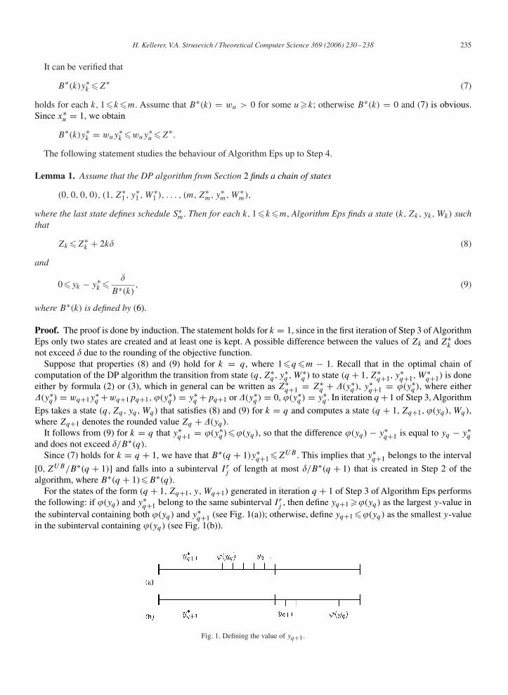
algorithm, where B∗(q + 1)�B∗(q).For the states of the form (q + 1, Zq+1, y, Wq+1) generated in iteration q + 1 of Step 3 of Algorithm Eps performs

the following: if �(yq) and y∗q+1 belong to the same subinterval I r

j , then define yq+1 ��(yq) as the largest y-value inthe subinterval containing both �(yq) and y∗

q+1 (see Fig. 1(a)); otherwise, define yq+1 ��(yq) as the smallest y-valuein the subinterval containing �(yq) (see Fig. 1(b)).

Fig. 1. Defining the value of yq+1.


It is clear that the state (q + 1, Zq+1, yq+1, Wq+1) will be stored and y∗q+1 �yq+1. Moreover, if yq+1 and y∗

q+1belong to the same subinterval I r

j then yq+1 − y∗q+1 ��/B∗(q + 1) (see Fig. 1(a)); otherwise, y∗

q+1 is closer to yq+1

than to �(yq), i.e., yq+1 − y∗q+1 ��(yq) − y∗

q+1 ��/B∗(q)��/B∗(q + 1) (see Fig. 1(b)). Thus, (9) follows.If �(y∗

q ) = wq+1(y∗q +pq+1), so that x∗

q+1 = 1 and B∗(q)�wq+1, we use properties (8) and (9) for k = q to derive

Zq+1 � Zq + wq+1(yq + pq+1) + �

� (Z∗q + 2q�) + wq+1

((y∗q + �

B∗(q)

)+ pq+1

)+ �

= (Z∗q + wq+1(y

∗q + pq+1)) + wq+1

(�

B∗(q)

)+ (2q + 1)�

� Z∗q+1 + wq+1

(�

wq+1

)+ (2q + 1)� = Z∗

q+1 + (2q + 2)�.

Otherwise, if �(y∗q ) = 0, we obtain Zq+1 = Zq . In any case, the inequalities (8) and (9) hold for k = q + 1. �

Now we prove that Algorithm Eps provides a required accuracy.

Lemma 2. Assume a job with the processing time p and the weight w is straddling in a schedule S∗ that is optimalfor problem 1|dj = d|∑wjTj . Given a positive �, Algorithm Eps outputs a schedule S� = S�(p, w) with the functionvalue Z�(p, w) such that

Z�(p, w) − Z∗ ��Z∗,

where Z∗ = Z(S∗).

Proof. Recall that schedule S∗ = S∗(p, w) can be obtained by inserting the straddling job into some schedule S∗m

that is feasible for problem 1|(p, w), dj = dstop|∑wjTj . As in Lemma 1, let (m, Z∗m, y∗

m, W ∗m) be a state that defines

schedule S∗m. Define x∗ by formula (4) with ym = y∗

m. It follows that

Z∗ = Z(S∗(p, w)) = Z∗m + (W ∗

m + w)px∗. (10)

Due to Lemma 1, having performed Step 3,Algorithm Eps will find a state (m, Zm, ym, Wm) such that Zm−Z∗m �2m�

and ym �y∗m. This state defines a feasible schedule for problem 1|(p, w), dj = dstop|∑wjTj , since all early jobs can

be completed by time Am − ym �Am − y∗m �d .

Comparing Wm and W ∗m, recall that in each iteration the W -values are related neither to the Z-values nor to the

y-values computed, so that the computation path that leads to Wm contains no more than m rounding operations.We show that the inequality

Wk �W ∗k

(1 + �

2

)k/m

(11)

holds for each k = 1, . . . , m. It is true for k = 1, since in the first iteration at most one state with a non-zero W -valuewill be found.

Suppose that (11) holds for each k, 1�k�q. We only need to consider the case that job q + 1 is scheduled late;otherwise Wq+1 = Wq . Due to rounding up Wq + wq+1 to the nearest power of (1 + �

2 )1/m, we get

Wq+1 �(Wq + wq+1)(

1 + �

2

)1/m

�(

W ∗q

(1 + �

2

)q/m + wq+1

)(1 + �

2

)1/m

�W ∗q+1

(1 + �

2

)(q+1)/m

.

Applying (11) for k = m, we derive that

W ∗m �Wm �W ∗

m

(1 + �

2

). (12)

Let Z�(p, w) denote the smallest value of the objective function found by Algorithm Eps for the chosen straddlingjob. It follows that

Z�(p, w)�Zm + p(Wm + w)x,


where x is defined by (4). Note that the case that x < 0 is excluded from consideration, since the chosen straddling jobcan be inserted in such a way that it completes strictly before the due date, and this means that in an optimal scheduleanother job is straddling.

Since ym �y∗m due to (9), it follows that x < x∗. Due to (8), (10) and (12), we derive

Z�(p, w) � (Z∗m + 2m�) + (Wm + w)px∗

� Z∗m + �

2ZLB +

(W ∗

m

(1 + �

2

)+ w

)px∗

= Z∗ + �

2ZLB + �

2pW ∗

mx∗

� Z∗(1 + �),

and the lemma holds. �

To complete our analysis, we estimate the running time of Algorithm Eps. First, notice that the total number of thesubintervals created in Step 2 does not exceed m(ZUB/�), because each interval Iu, 1�u�h, is split into subintervalsof length �/w�(u), so that

ZUB

w�(1)

× w�(1)

�+

h∑u=2

[ZUB

w�(u)

− ZUB

w�(u−1)

]w�(u)

��

h∑u=1

ZUB

w�(u)

× w�(u)

��h

ZUB

��m

ZUB

�.

In some iteration k, 0�k�m − 1, of Step 3 the states with no more than ZUB/� distinct values of the objectivefunction are originally created due to the rounding. Using W, the sum of all weights, as an upper bound on values Wk

computed in each iteration, we observe that the number of rounded W -values does not exceed n log1+�/2 W , which isof order O((n log W)/�) and hence polynomial in the length of the encoded input.

By definition of � we have that

ZUB

�= 2ZLB

�� 8n

�= O

(n

�

).

In each iteration k, for each pair (Zk, Wk) at most two states are kept in each of at most n(ZUB/�) = O(n2/�)subintervals. Thus, in each iteration of Step 3 at most O((n2(n/�)2 log W)/�) states are created and stored and a typicaliteration of Step 3 can be implemented in O((n4 log W)/�3) time.

Since for each choice of the straddling job finding an approximate solution includes n − 1 iterations of Step 3, andStep 4 does not increase the overall running time, we deduce that our algorithm requires at most O((n6 log W)/�3)

time.We summarize our main result as the following statement.

Theorem 1. For problem 1|dj = d|∑wjTj there exists an FPTAS with the running time O((n6 log W)/�3), where Wis the total sum of all weights.

4. Conclusion

In this paper we present a fully polynomial approximation scheme (FPTAS) for the problem of minimizing theweighted total tardiness on a single machine about a common due date, thereby resolving a question raised in [7]. Therunning time of our FPTAS is not strongly polynomial in the length of input; it remains to be seen whether an FPTAScan be designed with the running time that is only polynomial in n and 1/�.

Another interesting research goal is to extend our scheme to handle the problem with any fixed number of distinctdue dates.

Acknowledgement

We are grateful to an anonymous referee for the comments that have helped clarify the proof of Lemma 1.


References

[1] T.S.Abdul-Razaq, C.N. Potts, L.N. Van Wassenhove,A survey of algorithms for the single machine total weighted tardiness scheduling problem,Discrete Appl. Math. 26 (1990) 235–253.

[2] T.C.E. Cheng, C.T. Ng, J.J. Yuan, Z.H. Liu, Single machine scheduling to minimize total weighted tardiness, Eur. J. Oper. Res. 165 (2005)423–443.

[3] R.K. Congram, C.N. Potts, S.L. van de Velde, An iterated dynasearch algorithm for the single-machine total weighted tardiness schedulingproblem, INFORMS J. Comput. 14 (2002) 52–67.

[4] F. Della Croce, A. Grosso, V.T. Paschos, Lower bounds on the approximation ratios of leading heuristics for the single-machine total tardinessproblem, J. Scheduling 7 (2004) 85–91.

[5] J. Du, J.Y.-T. Leung, Minimizing total tardiness on one machine is NP-hard, Math. Oper. Res. 15 (1990) 483–495.[6] Y. Fathi, H.W.L. Nuttle, Heuristics for the common due date weighted tardiness problem, IIE Trans. 22 (1990) 215–225.[7] S.V. Kolliopoulos, G. Steiner, Approximation algorithms for minimizing the total weighted tardiness on a single machine, Theoret. Comput.

Sci. 355 (2006) 261–273.[8] E.L. Lawler, A ‘pseudopolynomial’ algorithm for sequencing jobs to minimize total tardiness, Ann. Discrete Math. 1 (1977) 331–342.[9] E.L. Lawler, A fully polynomial approximation scheme for the total tardiness problem, Oper. Res. Lett. 1 (1982) 207–208.

[10] E.L. Lawler, J.M. Moore, A functional equation and its application to resource allocation and sequencing problems, Management Sci. 16 (1969)77–84.

[11] J.K. Lenstra, A.H.G. Rinnooy Kan, P. Brucker, Complexity of machine scheduling problems, Ann. Discrete Math. 1 (1977) 343–362.[12] C.N. Potts, L.N. Van Wassenhove, A branch and bound algorithm for the total weighted tardiness problem, Oper. Res. 33 (1985) 363–377.[13] T. Sen, J.M. Sulek, P. Dileepan, Static scheduling research to minimize weighted and unweighted tardiness: a state-of-the-art survey, Int.

J. Production Econom. 83 (2003) 1–12.[14] W.E. Smith, Various optimizers for single stage production, Naval Res. Logist. Quart. 3 (1956) 59–66.[15] J. Yuan, The NP-hardness of the single machine common due date weighted tardiness problem, Systems Sci. Math. Sci. 5 (1992) 328–333.

Documents

A fully polynomial approximation scheme for the single machine weighted total tardiness problem with a common due date