Embed Size (px)
Citation preview
CONGESTION PRICING AND NON-COOPERATIVE GAMES IN
COMMUNICATION NETWORKS
AYALVADI GANESH
Microsoft Research, 7 J J Thompson Avenue, Cambridge CB3 0FB, UK,
KOENRAAD LAEVENS
Ghent University, Sint-Pietersnieuwstraat 41, B-9000 Ghent, Belgium,
RICHARD STEINBERG
University of Cambridge, Judge Business School, Cambridge CB2 1AG, UK,
Abstract
We consider congestion pricing as a mechanism for sharing bandwidth in
communication networks, and model the interaction among the users as a
game. We propose a decentralized algorithm for the users that is based on
the history of the price process, where user response to congestion prices is
analogous to “fictitious play” in game theory, and show that this results in
convergence to the unique Wardrop equilibrium. We further show that the
Wardrop equilibrium coincides with the welfare maximizing capacity allo-
cation.
Received xxx; accepted March 2006.
Subject classifications: Communications: computer networks. Games: non-
cooperative.
Area of review: Telecommunications

1 Introduction
The problem of sharing bandwidth among users in a communication network has
been the focus of much recent research. For early work, see Kelly, Maulloo, and
Tan (1998), Gibbens and Kelly (1999), and Low and Lapsley (1999), and for
a recent overview see Srikant (2004). Centralized solutions to this problem are
impractical in large networks serving very diverse users. This motivates shifting
the burden of rate allocation from the network to the end-systems. We propose a
new decentralized scheme for user adaptation.
In this paper, the termuserrefers to an instance of an application like e-mail
or web transfer running on a computer (the end-system) connected to the Internet.
The majority of applications on the Internet employ TCP (Transmission Control
Protocol) to adjust their transmission rates. In TCP, the receiver sends an acknowl-
edgement of each received packet to the sender. The network will drop packets
when it is congested. Each sender continually increases its transmission rate un-
til it fails to receive an acknowledgement, whereupon it assumes the network is
congested and cuts back its sending rate.
Dropped packets are both inefficient and late as indicators of congestion. This
forces users to sharply adapt their transmission rates, resulting in rate oscillation
and reduced throughput. An indicator of incipient congestion that avoids packet
drops could achieve higher network utilization. This is the motivation of ECN
(Explicit Congestion Notification) (Ramakrishnan and Jain (1990), Floyd (1994)),
wherein the network routers and switches provide early congestion feedback by
marking packets. The marks are returned to the sender with the acknowledgement
of the receipt of a packet.
A broader problem with TCP, which is not addressed by ECN, is that it makes
2
no explicit attempt to discriminate between users on the basis of differing appli-
cation requirements; nevertheless, there is implicit discrimination on the basis of
network characteristics (such as round-trip time for the connection) because of
properties of the feedback loop employed by TCP. In practice, users have very
different requirements and it would be desirable for the network to provide a dif-
ferentiated service that is responsive to these different requirements. It is hard to
see how to do this in a coherent manner without introducing differentiated charges.
Indeed, in the absence of such charges, users would have no incentive to honestly
reveal their requirements. By reflecting the social costs imposed by a user, charges
can also serve to discourage rate adaptation strategies that may be individually
beneficial but socially harmful.
Gibbens and Kelly (1999) have proposed a simple and innovative mecha-
nism to implement usage-based charging. Their scheme is scalable in the sense
that it does not require core network routers to keep track of individual source-
destination pairs but only of aggregate traffic. Prices are set on the basis of ag-
gregate traffic and communicated periodically to users, who can then decide for
themselves how to best satisfy their requirements at the given price. One way
to communicate price feedback is by modifying ECN to carry prices instead of
marks indicating congestion.
Kelly, Maulloo, and Tan (1998) proposed a scheme for users to individually
adapt their rates based on price feedback and showed that, under certain condi-
tions, this mechanism converges in the long run to a socially optimal allocation
of bandwidth. Users were modelled as having a utility function that is additively
separable over time, and increasing and concave in the instantaneous bandwidth
they receive (see Shenker (1995)). Such users have been termedelastic. A key
3

idea in the work of Kelly et al. is to view user adaptation as a distributed gradient
ascent algorithm for maximizing social welfare. Consequently, the social welfare
function serves as a Lyapunov function for the dynamics. This work was extended
by Johari and Tan (2001), who studied the stability of the same dynamics but in-
cluding feedback delays.
An approach based on solving thedual to the welfare maximization problem
has been studied by Low and Lapsley (1999). Here, the network adapts prices
based on observed aggregate demand, and users attempt to maximize their instan-
taneous utility based on the price feedback they receive. Users are myopic in that
they attempt to maximize their utility without taking account of the likely response
of other users to the common price information. Low and Lapsley (1999) show
that, if the network adjusts prices sufficiently slowly, the system again converges
to the welfare maximizing allocation. Kunniyur and Srikant (2001) considered a
model wherein the users adapt their transmission rates on a fast timescale while
the network adapts its marking function (which could be interpreted as a price) on
a slow timescale. They studied convergence subject to an assumption of separa-
tion of timescales.
In this paper, we model theinteractionbetween users as a game, and show that
a Nash equilibrium of this game coincides (in a large system) with the welfare
maximizing solution of the frameworks studied by Kelly, Maulloo, Tan (1998)
and Low and Lapsley (1999). We also present a model ofuser responseto con-
gestion prices that is very similar to “fictitious play” in game theory, and show
that this user behavior results in convergence to the aforementioned Nash equi-
librium. In our model, users attempt to maximize instantaneous utility based on
their expectationsof the price, where expectations are formed adaptively based
4
on the history of the price process. In fictitious play, each player selects a best
response to the empirical distribution of actions of his opponents (Fudenberg and
Levine (1998)). Here, these actions only impact each player through the price;
if, in addition, players are risk neutral, then it suffices that they choose their ac-
tions as a best response to a (weighted) average of past prices, as we suggest in
this paper. The practical implementation of pricing schemes might involve band-
width brokers who act as intermediaries between network service providers and
end users. Anderson, Kelly, and Steinberg (2006) describe one way to set up such
an intermediary service.
The game-theoretic formulation in this paper differs from the work cited above,
and is intended to reflect strategies that might be adopted by self-interested users.
In order to model feedback delays, we employ a discrete-time formulation. The
resulting dynamical system is significantly different from that in Kelly et al. and
also that in Low and Lapsley; in particular, it does not possess a natural candi-
date for a Lyapunov function, and it is not the gradient of any scalar function.
(Indeed, Lyapunov functions cannot generally be found for systems with delayed
feedback; e.g., Massoulie (2002) and Vinnicombe (2002), who studied extensions
of Kelly et al.’s model with feedback delays, rely on techniques other than Lya-
punov functions to establish stability. Srikant (2004) also discusses the technical
difficulties in proving convergence when feedback is not instantaneous.) Hence,
we rely on different techniques based on contraction mappings to prove conver-
gence of the dynamics; furthermore, we show that the unique equilibrium for the
dynamics generated by the users’ adaptation to prices, starting from arbitrary ini-
tial conditions, is the welfare-maximizing allocation, which is also the Wardrop
equilibrium of the game; it coincides with the Nash equilibrium in a large system
5

limit.
The rest of the paper is organized as follows. In Section 2, we model as a
game the utility maximization problem of individual users. We also discuss some
of the informational issues, make some observations about equilibria, and place
our work within the context of well-known models of competition. This frame-
work helps to motivate theadaptive expectationsapproach that we develop in
Section 3. In Section 3, we derive conditions under which this model of adap-
tation leads the users to converge to a socially optimal allocation of bandwidth;
in addition, we determine the speed of convergence. The results of this paper in
more detail are as follows. Lemma1 uses Brouwer’s fixed point theorem to show
existenceanduniquenessof a price that is self-consistent in the following sense:
if all the players have it as theirpredictedprice, and choose their transmission
rate accordingly, then the resulting price coincides with the prediction. We also
show how the functional form of the pricing function is connected with queue-
ing phenomena at the link. We then establish conditions that ensure convergence
from arbitrary initial conditions to the self-consistent price. In particular, Lemma
2 shows that the price expectations of the players will be bounded and will con-
verge to the (unique) fixed point. As we are taking expectations over the history
of the process, we then in Theorems1 and2 provide conditions on the associated
averaging parameter such that geometric convergence to the fixed point is ensured
from any initial condition. Finally, Lemma3 gives a sufficient and another neces-
sary condition such that the hypothesis of the previous Theorem does indeed hold.
In Section 4, we present conclusions along with suggestions for future work. All
proofs of lemmas and theorems appear in the appendix.
6
2 Model
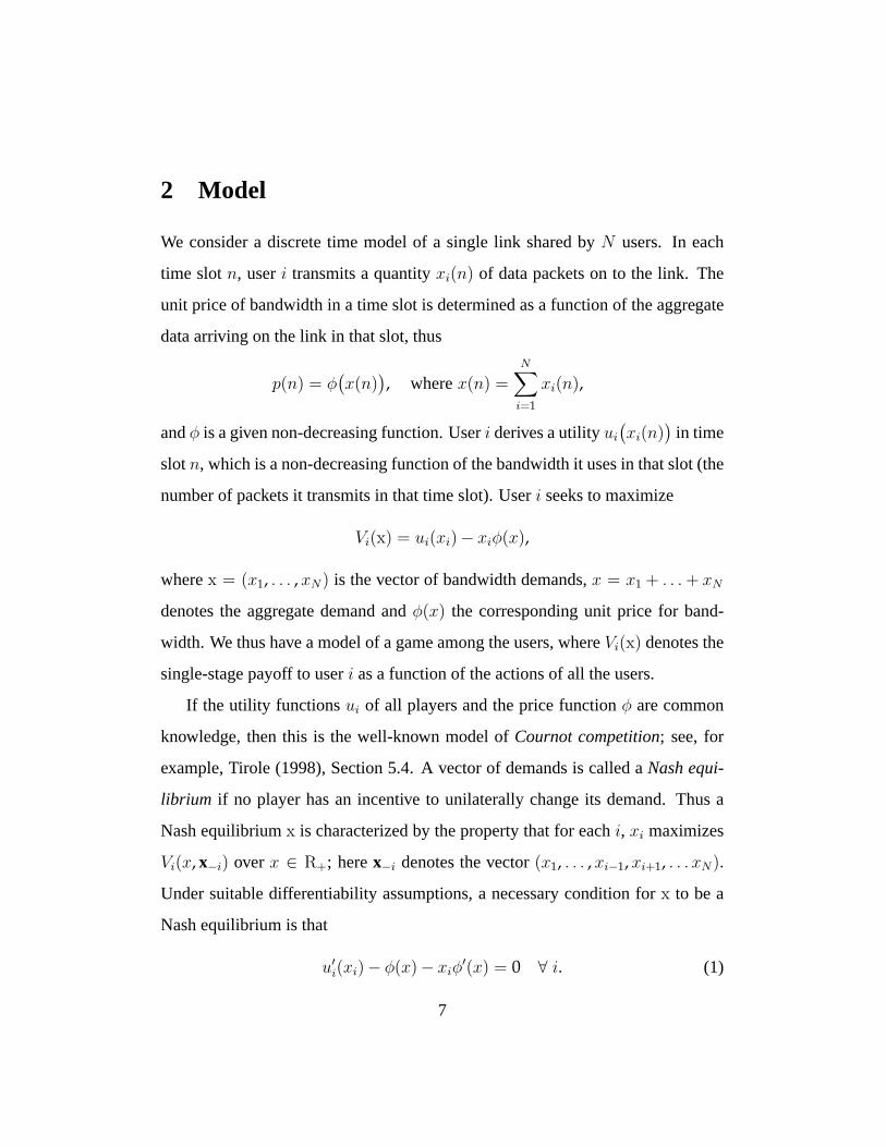
We consider a discrete time model of a single link shared byN users. In each
time slotn, useri transmits a quantityxi(n) of data packets on to the link. The
unit price of bandwidth in a time slot is determined as a function of the aggregate
data arriving on the link in that slot, thus
p(n) = φ(x(n)
), wherex(n) =
N∑i=1
xi(n),
andφ is a given non-decreasing function. Useri derives a utilityui(xi(n)
)in time
slotn, which is a non-decreasing function of the bandwidth it uses in that slot (the
number of packets it transmits in that time slot). Useri seeks to maximize
Vi(x) = ui(xi)− xiφ(x),
wherex = (x1, . . . ,xN) is the vector of bandwidth demands,x = x1 + . . .+ xN
denotes the aggregate demand andφ(x) the corresponding unit price for band-
width. We thus have a model of a game among the users, whereVi(x) denotes the
single-stage payoff to useri as a function of the actions of all the users.
If the utility functionsui of all players and the price functionφ are common
knowledge, then this is the well-known model ofCournot competition; see, for
example, Tirole (1998), Section 5.4. A vector of demands is called aNash equi-
librium if no player has an incentive to unilaterally change its demand. Thus a
Nash equilibriumx is characterized by the property that for eachi, xi maximizes
Vi(x, x−i) overx ∈ R+; herex−i denotes the vector(x1, . . . ,xi−1,xi+1, . . . xN).
Under suitable differentiability assumptions, a necessary condition forx to be a
Nash equilibrium is that
u′i(xi)− φ(x)− xiφ′(x) = 0 ∀ i. (1)
7
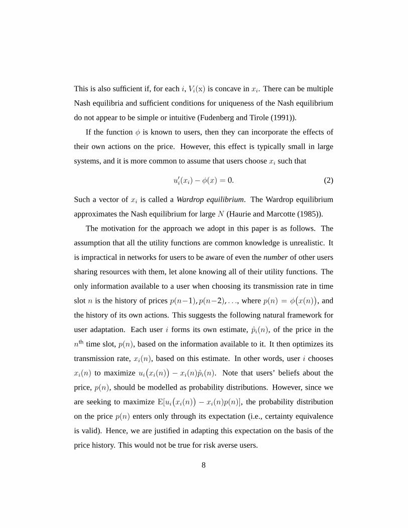
This is also sufficient if, for eachi, Vi(x) is concave inxi. There can be multiple
Nash equilibria and sufficient conditions for uniqueness of the Nash equilibrium
do not appear to be simple or intuitive (Fudenberg and Tirole (1991)).
If the functionφ is known to users, then they can incorporate the effects of
their own actions on the price. However, this effect is typically small in large
systems, and it is more common to assume that users choosexi such that
u′i(xi)− φ(x) = 0. (2)
Such a vector ofxi is called aWardrop equilibrium. The Wardrop equilibrium
approximates the Nash equilibrium for largeN (Haurie and Marcotte (1985)).
The motivation for the approach we adopt in this paper is as follows. The
assumption that all the utility functions are common knowledge is unrealistic. It
is impractical in networks for users to be aware of even thenumberof other users
sharing resources with them, let alone knowing all of their utility functions. The
only information available to a user when choosing its transmission rate in time
slot n is the history of pricesp(n−1), p(n−2), . . ., wherep(n) = φ(x(n)
), and
the history of its own actions. This suggests the following natural framework for
user adaptation. Each useri forms its own estimate,pi(n), of the price in the
nth time slot,p(n), based on the information available to it. It then optimizes its
transmission rate,xi(n), based on this estimate. In other words, useri chooses
xi(n) to maximizeui(xi(n)
)− xi(n)pi(n). Note that users’ beliefs about the
price,p(n), should be modelled as probability distributions. However, since we
are seeking to maximizeE[ui(xi(n)
)− xi(n)p(n)], the probability distribution
on the pricep(n) enters only through its expectation (i.e., certainty equivalence
is valid). Hence, we are justified in adapting this expectation on the basis of the
price history. This would not be true for risk averse users.
8

As noted earlier, the model we study in this paper corresponds to Cournot
competition. Another commonly used model of oligopolistic competition is the
Bertrand model, in which each producer of an undifferentiated good sets a price
and is willing to supply any demand at that price. Consumers choose the quantity
demanded based on the market price, which is obviously the lowest of the prices
offered by the different producers. In our context, this model corresponds to each
user specifying a price it is willing to pay per unit bandwidth, i.e., per packet. If
the user can generate arbitrarily high demand at this price, then the network ac-
cepts only the user with the highest bid. More realistically, the demand from each
user would be bounded, in which case the network would accept packets from
a collection of highest bidders. This corresponds precisely to the smart market
model that was proposed by Mackie-Mason and Varian (1996), where users at-
tach a bid to each packet that is the maximum price they are willing to pay for
its transmission. The network admits packets in decreasing order of bids until
capacity is reached. Each admitted packet is charged the amount of the highest
rejected bid (or zero if all packets are admitted). While this scheme is efficient
in an economic sense, it is impractical for a number of reasons. One is the sheer
difficulty of conducting repeated auctions at the speeds dictated by high-capacity
networks. Another issue is the fairness of comparing bids on a packet that has
freshly entered the network with one that has been waiting its turn for a long time.
The model of congestion pricing we study does not suffer from these problems.
9
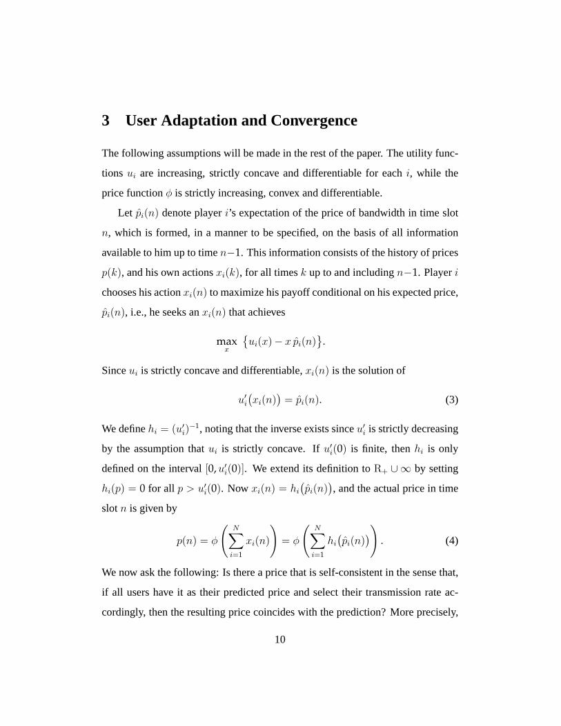
3 User Adaptation and Convergence
The following assumptions will be made in the rest of the paper. The utility func-
tions ui are increasing, strictly concave and differentiable for eachi, while the
price functionφ is strictly increasing, convex and differentiable.
Let pi(n) denote playeri’s expectation of the price of bandwidth in time slot
n, which is formed, in a manner to be specified, on the basis of all information
available to him up to timen−1. This information consists of the history of prices
p(k), and his own actionsxi(k), for all timesk up to and includingn−1. Playeri
chooses his actionxi(n) to maximize his payoff conditional on his expected price,
pi(n), i.e., he seeks anxi(n) that achieves
maxx
{ui(x)− x pi(n)
}.
Sinceui is strictly concave and differentiable,xi(n) is the solution of
u′i(xi(n)
)= pi(n). (3)
We definehi = (u′i)−1, noting that the inverse exists sinceu′i is strictly decreasing
by the assumption thatui is strictly concave. Ifu′i(0) is finite, thenhi is only
defined on the interval[0,u′i(0)]. We extend its definition toR+ ∪∞ by setting
hi(p) = 0 for all p > u′i(0). Now xi(n) = hi(pi(n)
), and the actual price in time
slotn is given by
p(n) = φ
(N∑i=1
xi(n)
)= φ
(N∑i=1
hi(pi(n)
)). (4)
We now ask the following: Is there a price that is self-consistent in the sense that,
if all users have it as their predicted price and select their transmission rate ac-
cordingly, then the resulting price coincides with the prediction? More precisely,
10

is there aq∗ such that
q∗ = φ(∑N
i=1 hi(q∗))
. (5)
The answer is yes, by Brouwer’s fixed point theorem (see Varian (1992), for ex-
ample), as we now show.
Lemma 1 Suppose the utility functionsui are strictly concave, increasing and
differentiable for eachi, and that the price functionφ is continuous and increas-
ing.
Let hi be defined as above. Then, the functionq 7→ φ(∑N
i=1 hi(q))
has a
fixed point. In other words, there is a self-consistent priceq∗ such thatq∗ =
φ(∑N
i=1 hi(q∗))
. Moreover, the fixed pointq∗ is unique. 2
We have thus established theexistenceand uniquenessof a self-consistent
price in the sense described above. In general, it is not clear whether the process
of user adaptationconvergesto the fixed point from arbitrary initial conditions.
We shall now investigate this question in a specific model of adaptation.
Suppose players make use of a one-step error correction mechanism for pre-
diction, which corresponds to using an exponentially weighted moving average
estimator. Specifically, let the assumed model of user expectation formation be
pi(n+1) = pi(n) + αi[p(n)− pi(n)
]=
n∑k=0
(1− αi)kαip(n− k) + (1− αi)n+1pi(0), (6)
where theαi are given constants, and it is assumed that1− αi ∈ (0, 1) for all i.
Our aim is to show that, asn tends to infinity,p(n) andpi(n), for eachi, converge
to the self-consistent price,q∗.
11
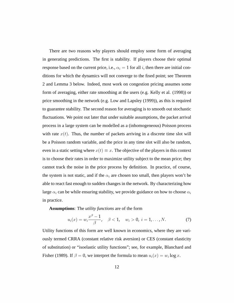
There are two reasons why players should employ some form of averaging
in generating predictions. The first is stability. If players choose their optimal
response based on the current price, i.e.,αi = 1 for all i, then there are initial con-
ditions for which the dynamics will not converge to the fixed point; see Theorem
2 and Lemma 3 below. Indeed, most work on congestion pricing assumes some
form of averaging, either rate smoothing at the users (e.g. Kelly et al. (1998)) or
price smoothing in the network (e.g. Low and Lapsley (1999)), as this is required
to guarantee stability. The second reason for averaging is to smooth out stochastic
fluctuations. We point out later that under suitable assumptions, the packet arrival
process in a large system can be modelled as a (inhomogeneous) Poisson process
with ratex(t). Thus, the number of packets arriving in a discrete time slot will
be a Poisson random variable, and the price in any time slot will also be random,
even in a static setting wherex(t) ≡ x. The objective of the players in this context
is to choose their rates in order to maximize utility subject to the mean price; they
cannot track the noise in the price process by definition. In practice, of course,
the system is not static, and if theαi are chosen too small, then players won’t be
able to react fast enough to sudden changes in the network. By characterizing how
largeαi can be while ensuring stability, we provide guidance on how to chooseαi
in practice.
Assumptions: Theutility functionsare of the form
ui(x) = wixβ − 1β
, β < 1, wi > 0, i = 1, . . . ,N . (7)
Utility functions of this form are well known in economics, where they are vari-
ously termed CRRA (constant relative risk aversion) or CES (constant elasticity
of substitution) or “isoelastic utility functions”; see, for example, Blanchard and
Fisher (1989). Ifβ = 0, we interpret the formula to meanui(x) = wi logx.
12
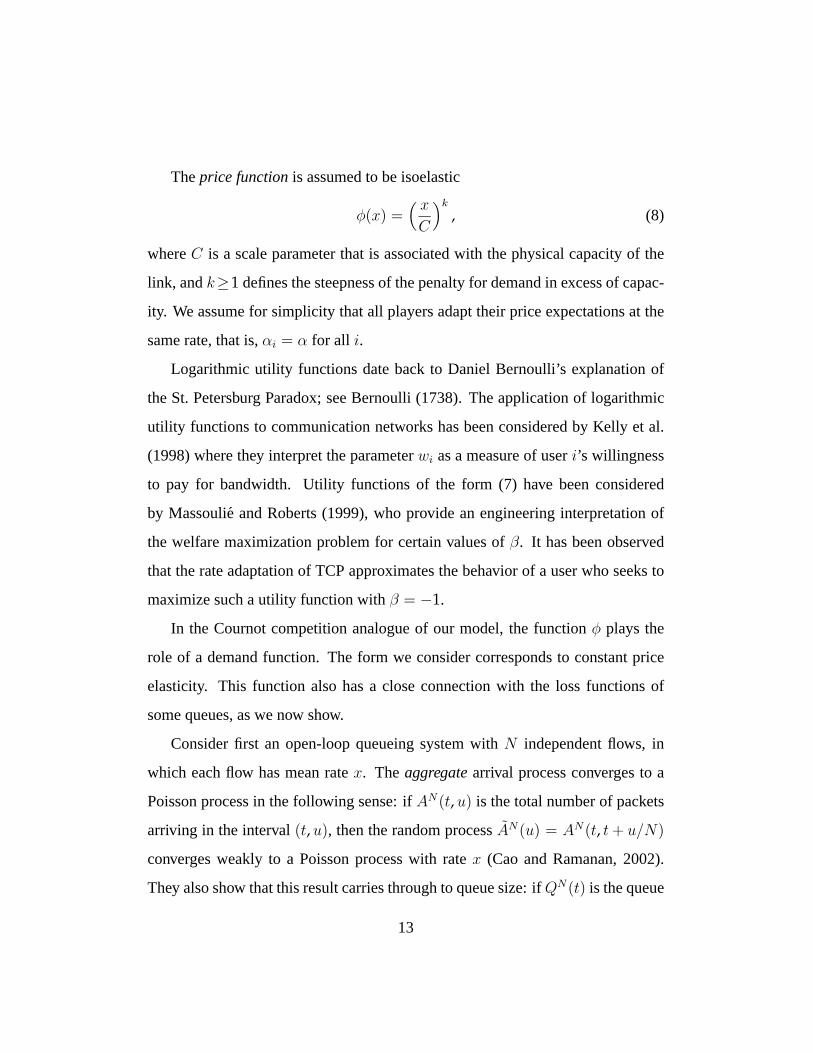
Theprice functionis assumed to be isoelastic
φ(x) =( xC
)k, (8)
whereC is a scale parameter that is associated with the physical capacity of the
link, andk≥1 defines the steepness of the penalty for demand in excess of capac-
ity. We assume for simplicity that all players adapt their price expectations at the
same rate, that is,αi = α for all i.
Logarithmic utility functions date back to Daniel Bernoulli’s explanation of
the St. Petersburg Paradox; see Bernoulli (1738). The application of logarithmic
utility functions to communication networks has been considered by Kelly et al.
(1998) where they interpret the parameterwi as a measure of useri’s willingness
to pay for bandwidth. Utility functions of the form (7) have been considered
by Massoulie and Roberts (1999), who provide an engineering interpretation of
the welfare maximization problem for certain values ofβ. It has been observed
that the rate adaptation of TCP approximates the behavior of a user who seeks to
maximize such a utility function withβ = −1.
In the Cournot competition analogue of our model, the functionφ plays the
role of a demand function. The form we consider corresponds to constant price
elasticity. This function also has a close connection with the loss functions of
some queues, as we now show.
Consider first an open-loop queueing system withN independent flows, in
which each flow has mean ratex. Theaggregatearrival process converges to a
Poisson process in the following sense: ifAN(t,u) is the total number of packets
arriving in the interval(t,u), then the random processAN(u) = AN(t, t+ u/N)
converges weakly to a Poisson process with ratex (Cao and Ramanan, 2002).
They also show that this result carries through to queue size: ifQN(t) is the queue
13

size at timet, then the distribution ofQN(t) converges to that for a queue fed by
a Poisson process with arrival ratex and served at constant rateC, in an infinite-
buffer system, assumingx < C. We expect that this result can be extended to a
system with a finite bufferB, and tox ≥ C. The loss probability for a finite-buffer
open-loop queue is thus
p = LB(x/C),
whereLB can be calculated by finding the equilibrium distribution of a suitable
Markov chain.
Suppose next that the source ratesx vary over time, but “slowly.” It is known
thatQN(t) makes excursions of sizeO(1) in timescaleO(1/N) (Raina and Wis-
chik (2005)). Therefore, in any short interval(t, t+ δ), the queue size will repeat-
edly hit empty and full. This suggests that, if the mean arrival ratex(t) does not
change by much in the interval(t, t+ δ), the loss probability is
p(t) = LB(ρ(t)), (9)
whereρ(t) = x(t)/C. So, for example, if the resource were modelled as an
M/M/1 queue with service rateC packets per unit time, at which a packet is
marked with a congestion signal if it arrives at the queue to find at leastB packets
already present, this would yield
p(x) =( xC
)B.
Thus, our price functionφ can be motivated as being proportional to the packet
loss probability for a given aggregate arrival rate.
Recall that an objective of the pricing scheme is to avoid packet drops by
signalling incipient congestion. Therefore, links should set prices in a manner
14
that ensures that aggregate demand does not exceed the physical capacity of the
link for extended periods of time; this may involve settingC in the price function
(8) to be some fraction, such as 90%, of the actual link capacity. The parameterC
can be set, for instance, using an adaptive scheme; the idea is to adjustC on a slow
time scale in order to achieve a desired trade-off between high link utilization and
low packet drop probability. A similar idea has been proposed and analyzed by
Kunniyur and Srikant (2001) in a related context.
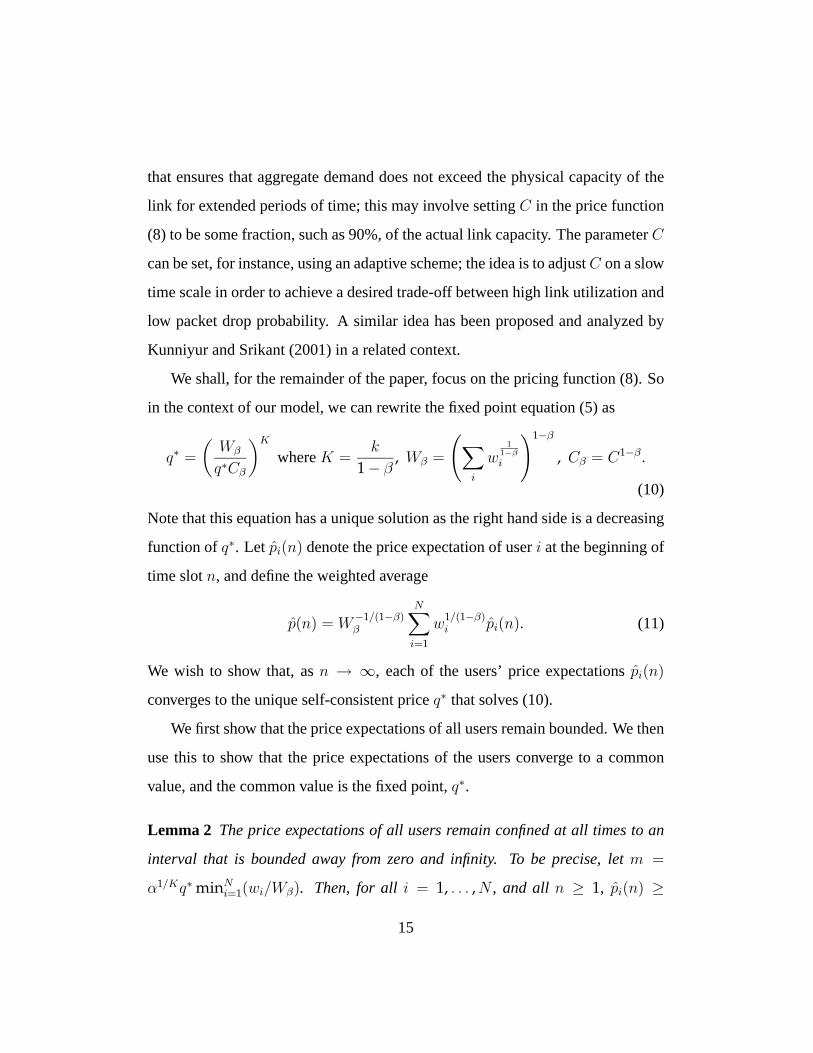
We shall, for the remainder of the paper, focus on the pricing function (8). So
in the context of our model, we can rewrite the fixed point equation (5) as
q∗ =
(Wβ
q∗Cβ
)KwhereK =
k
1− β, Wβ =
(∑i
w1
1−βi
)1−β
, Cβ = C1−β .
(10)
Note that this equation has a unique solution as the right hand side is a decreasing
function ofq∗. Let pi(n) denote the price expectation of useri at the beginning of
time slotn, and define the weighted average
p(n) = W−1/(1−β)β
N∑i=1
w1/(1−β)i pi(n). (11)
We wish to show that, asn → ∞, each of the users’ price expectationspi(n)
converges to the unique self-consistent priceq∗ that solves (10).
We first show that the price expectations of all users remain bounded. We then
use this to show that the price expectations of the users converge to a common
value, and the common value is the fixed point,q∗.
Lemma 2 The price expectations of all users remain confined at all times to an
interval that is bounded away from zero and infinity. To be precise, letm =
α1/Kq∗minNi=1(wi/Wβ). Then, for alli = 1, . . . ,N , and all n ≥ 1, pi(n) ≥
15
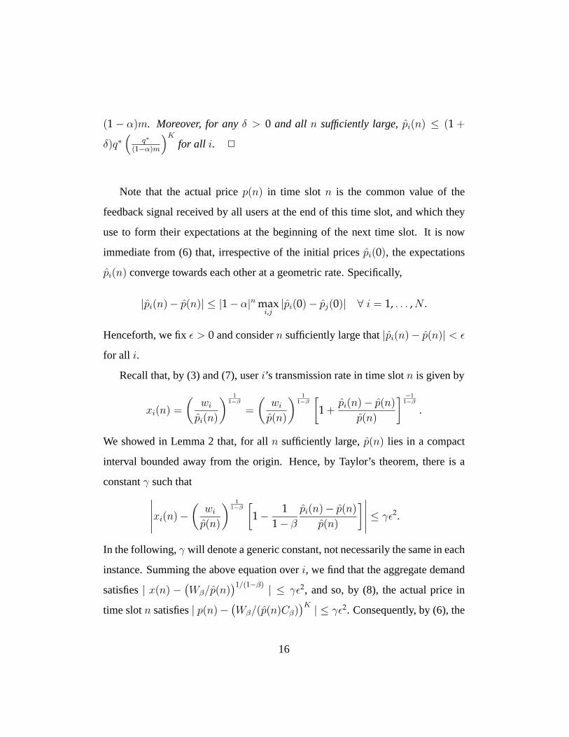
(1− α)m. Moreover, for anyδ > 0 and all n sufficiently large,pi(n) ≤ (1 +
δ)q∗(
q∗
(1−α)m
)Kfor all i. 2
Note that the actual pricep(n) in time slot n is the common value of the
feedback signal received by all users at the end of this time slot, and which they
use to form their expectations at the beginning of the next time slot. It is now
immediate from (6) that, irrespective of the initial pricespi(0), the expectations
pi(n) converge towards each other at a geometric rate. Specifically,
|pi(n)− p(n)| ≤ |1− α|n maxi,j|pi(0)− pj(0)| ∀ i = 1, . . . ,N .
Henceforth, we fixε > 0 and considern sufficiently large that|pi(n)− p(n)| < ε
for all i.
Recall that, by (3) and (7), useri’s transmission rate in time slotn is given by
xi(n) =
(wipi(n)
) 11−β
=
(wip(n)
) 11−β[
1 +pi(n)− p(n)
p(n)
] −11−β
.
We showed in Lemma 2 that, for alln sufficiently large,p(n) lies in a compact
interval bounded away from the origin. Hence, by Taylor’s theorem, there is a
constantγ such that∣∣∣∣∣xi(n)−(wip(n)
) 11−β[
1− 11− β
pi(n)− p(n)
p(n)
]∣∣∣∣∣ ≤ γε2.
In the following,γ will denote a generic constant, not necessarily the same in each
instance. Summing the above equation overi, we find that the aggregate demand
satisfies| x(n)−(Wβ/p(n)
)1/(1−β) | ≤ γε2, and so, by (8), the actual price in
time slotn satisfies| p(n)−(Wβ/(p(n)Cβ)
)K | ≤ γε2. Consequently, by (6), the
16
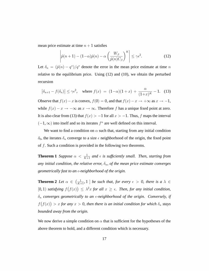
mean price estimate at timen+ 1 satisfies∣∣∣∣∣p(n+ 1)− (1−α)p(n)− α(
Wβ
p(n)Cβ
)K∣∣∣∣∣ ≤ γε2. (12)
Let δn = (p(n)− q∗)/q∗ denote the error in the mean price estimate at timen
relative to the equilibrium price. Using (12) and (10), we obtain the perturbed
recursion∣∣δn+1 − f(δn)∣∣ ≤ γε2, wheref(x) = (1−α)(1 + x) +
α
(1+x)K− 1. (13)
Observe thatf(x)−x is convex,f(0) = 0, and thatf(x)−x→ +∞ asx→ −1,
while f(x)− x → −∞ asx → ∞. Thereforef has a unique fixed point at zero.
It is also clear from (13) thatf(x) > −1 for all x > −1. Thus,f maps the interval
(−1,∞) into itself and so its iteratesfn are well defined on this interval.
We want to find a condition onα such that, starting from any initial condition
δ0, the iteratesδn converge to a sizeε neighborhood of the origin, the fixed point
of f . Such a condition is provided in the following two theorems.
Theorem 1 Supposeα < 1K+1 and ε is sufficiently small. Then, starting from
any initial condition, the relative error,δn, of the mean price estimate converges
geometrically fast to anε-neighborhood of the origin.
Theorem 2 Let α ∈(
1K+1 , 1 ] be such that, for everyε > 0, there is aλ ∈
[0, 1) satisfyingf(f(x)
)≤ λ2x for all x ≥ ε. Then, for any initial condition,
δn converges geometrically to anε-neighborhood of the origin. Conversely, if
f(f(x)
)> x for anyx > 0, then there is an initial condition for whichδn stays
bounded away from the origin.
We now derive a simple condition onα that is sufficient for the hypotheses of the
above theorem to hold, and a different condition which is necessary.
17
Lemma 3 Supposeα ∈ (0, 1), K > 1, and thatf is defined as in (13). IfαK ≤
1, then, for anyε > 0, there is aλ < 1 such thatf(f(x)
)≤ λ2x for all x > ε. On
the other hand, ifα(K + 1) > 2, then there is anx > 0 such thatf(f(x)
)≥ x.
Remark: Extensive numerical studies suggest that the conditionα(K + 1) ≤ 2
is both necessary and sufficient forf ◦ f to be a contraction, but we have not
been able to prove sufficiency. This condition is necessary and sufficient for local
stability of the liberalization of the above system around its equilibrium.
4 Conclusions
Congestion pricing has been proposed as a mechanism for reflecting the social
costs of congestion to users of the Internet. We considered the behavior of users
in the presence of congestion charges, and modelled the resulting interaction as
a game. We proposed a model of utility maximizing players in an environment
where prices are determined,ex post, by the collective actions of all. The players
attempt to predict prices based on their knowledge of the history of the price
process, and choose their actions to maximize their utility conditional on their
predictions. This is analogous to fictitious play in game theory. We found that,
under reasonable assumptions, this model of adaptation leads the system to an
efficient allocation: players’ price predictions converge to the actual price and
their bandwidth shares converge to levels that equalize their marginal utility of
bandwidth to the price of bandwidth.
A natural next step would be to extend the model and analysis to a general net-
work and, in particular, to model heterogeneous delays and user-specific smooth-
ing parameters for price prediction. It would also be interesting to examine the
18
effect different pricing functions may have on the interaction between users. Such
functions, which also have their genesis in queueing phenomena, serve as tem-
plates for “resource design,” which in turn help understand and meet Quality of
Service (QoS) requirements. Thus, their impact on network performance and user
behavior would be of interest to network service providers as well as software
vendors.
Acknowledgements
We are grateful to Frank Kelly and Gaurav Raina for helpful comments. Richard
Steinberg acknowledges support in part from the Communications Research Net-
work (CRN), a part of the Cambridge-MIT Institute (CMI).
Appendix
PROOF OFLEMMA 1: Definef : RN+ → [0, 1]N by
fi(p1, . . . , pN) =pi
1 + pi, i = 1, . . . ,n,
andΨ: RN+ → RN
+ by
Ψi(p1, . . . , pN) = φ
(N∑i=1
hi(pi(n)
)), i = 1, . . . ,N .
If Ψ has a fixed point, then it must necessarily be of the form(q∗, . . . , q∗) with
N identical components, and it is clear thatq∗ solves (5). Nowf is invertible
and it is not hard to see thatf ◦Ψ ◦ f−1 is a continuous map from the compact,
19

convex set[0, 1]N into itself. Thus, it has a fixed point,x ∈ [0, 1]N , by Brouwer’s
fixed point theorem. Note thatxi < 1 for all i = 1, . . . ,N ; if xi = 1, then the
ith component off ◦Ψ ◦ f−1(x) is zero, sincehi(∞) = 0 by definition, and sox
cannot be a fixed point. Thus, any fixed pointx of f ◦Ψ ◦ f−1 is in [0, 1)N , and
sof−1(x) ∈ RN . Clearlyf−1(x) is a fixed point ofΨ.
Next, if ui is strictly concave, thenu′i is decreasing, and so ishi = (u′i)−1.
Sinceφ is increasing, the functionx 7→ φ(h1(x), . . . ,hN(x)
)is decreasing. Thus,
it can have at most one fixed point, establishing uniqueness.2
PROOF OFLEMMA 2: Letn denote the first time, possibly0, at whichpi(n) < m
for somei. Then, by (3) and (7),xi(n) ≥ (wi/m)1/(1−β). Since the aggregate
demandx(n) is no smaller than the demand,xi(n), of useri, we obtain from (8)
that
p(n) ≥(
wimCβ
)K≥ 1α
(Wβ
q∗Cβ
)K=q∗
α,
where we have used the definition ofm to obtain the second inequality, and (10)
to obtain the last equality. Thus,pi(n+ 1) = (1−α)pi(n) +αp(n) ≥ q∗ for all i.
We have thus shown that, ifpi(n) < m for somei andn, thenpi(n+ 1) > m.
On the other hand, ifpi(n) ≥ m, thenpi(n+ 1) ≥ (1−α)m. This establishes the
first claim of the lemma.
Now, sincepi(n) ≥ (1− α)m for all i, it follows from (3) and (7) that
x(n) ≤(
Wβ
(1− α)m
)1/(1−β)
,
so that by (8)
p(n) ≤(
Wβ
(1− α)mCβ
)K=
(q∗
(1− α)m
)Kq∗.
20

Since this holds for alln, the second claim of the lemma is immediate from (6).
2
PROOF OFTHEOREM 1: We havef ′(x) = 1− α− αK(1+x)K+1 . NowαK ≤ 1− α
by assumption, so0 < f ′(x) < 1− α for all x > 0. Sincef(0) = 0, we get0 <
f(x) < (1− α)x for all x > 0. Chooseε small enough thatρ := 1− α− γε < 1.
Then, by (13),
−γε2 ≤ δn+1 ≤ ρδn ∀ δn > ε.
Thus, for initial conditionsδ0 > ε, δn converges geometrically at rateρ to the
interval[−γε2, ε].
Sincef is convex andf(0) = 0, the equationf(x) = 0 has at most one other
solution, which we denotex0. Observe thatx0 ≤ 0, becausef ′(0) ≥ 0. Now, for
x ∈ (x0, 0), we have by the convexity off that0 > f(x) > f(0) + xf ′(0) = λx,
whereλ = 1−α(K+1) ∈ [ 0, 1). Choosingε small enough thatρ := λ+ γε < 1,
we get
γε2 > δn+1 > ρδn ∀ δn ∈ (x0,−ε).
So, if the initial condition isδ0 ∈ (x0,−ε), thenδn converges geometrically at rate
ρ to the interval[−ε, γε2].
If δ0 ∈ (−1,x0 ], thenf(δ0) ≥ 0 by convexity, soδ1 ≥ −γε2. Thus, either
δ1 > ε and the previous argument applies to the initial conditionδ1, orδ1 is already
in anε-neighborhood of the origin.
Finally, we wish to show that once the iteratesδn enter anε-neighborhood of
the origin, they remain in this neighborhood. Recall thatf ′(0) = 1− α(K+1) ∈
[ 0, 1). Hence, for small enoughε, ρ := supx∈[−ε,ε] |f′(x)| < 1, and so|f(x)| < ρx
on [−ε, ε]. It is now immediate from (13) that, ifδn ∈ [−ε, ε], then so isδn+1. This
21
completes the proof of the theorem.2
PROOF OFTHEOREM 2: We have by (13) that∣∣δn+1 − f(δn)
∣∣ ≤ γε2 for all n.
We also showed in Lemma 2 thatp(n) is eventually confined to a compact set
bounded away from zero. Consequently,δn is confined to a compact set bounded
away from−1; on this set,f is differentiable and its derivative is bounded, sof is
Lipschitz. Hence,∣∣f(δn+1)− f(f(δn))
∣∣ ≤ γε2, for a possibly different constant,
γ. Thus, by the triangle inequality,∣∣δn+2 − f(f(δn))∣∣ ≤ ∣∣δn+2 − f(δn+1)
∣∣+ ∣∣f(δn+1)− f(f(δn))∣∣ ≤ γε2. (14)
Observe thatf ′(0) = 1− α(K + 1) is negative by assumption. Hence, by
convexity, f(x) ≥ 0 for all x ≤ 0. Moreover,f(x) → ∞ as x → ∞, so
there is anx0 > 0 such thatf(x0) = 0, f(x) < 0 on (0,x0) andf(x) > 0 on
(x0,∞). Now, if δn ∈ (0,x0), thenf(f(δn)
)> 0; moreover, ifδn ∈ (ε,x0), then
f(f(δn)
)< λ2δn < λ2x0. Combining this with (14), we see thatδn+2 < ρδn for
someρ < 1, and thatδn+2 ∈ (−γε2,x0). This implies that, if the initial condition
hasδ0 ∈ (0,x0), thenδ2n converges at a geometric rate to anε-neighborhood of
zero.
On the other hand, supposeδn > x0. Sincef ′(x) < 1− α for all x, f(x) =
f(x) − f(x0) < (1 − α)(x − x0) for all x > x0. Hence, by (13),δn+1 ∈
(−γε2, ρδn), for someρ < 1. Thus, if initially δ0 > x0, thenδn converges at
a geometric rate to the interval(−γε2,x0); onceδn is in this interval, the argu-
ment above is applicable. Finally, ifx < 0, thenf(x) > 0; hence, ifδ0 < 0, then
δ1 ∈ (−γε2,∞), and the arguments above are applicable.
Next, we show that, once the iteratesδn enter anε-neighborhood of the origin,
they remain confined to this neighborhood. We show in Lemma 3 below that, if
22
f ′(0) = 1− α(K + 1) < −1, then the hypothesis of the theorem cannot hold;
for small enoughx > 0, we will havef(f(x)
)> x. Hence, by assumption,
f ′(0) ∈ (−1, 0]. We can now use the same argument as in the proof of Lemma 1,
where we hadf ′(0) ∈ [0, 1).
It remains only to establish the converse. If we consider an initial condition
where all the price expectations,pi(0), are equal to each other (and hence top(0)),
then it is easy to verify that the recurrence (13) holds without the perturbation
term,γε2. Moreover, the price expectations of all users continue to be identical,
soδn+1 = f(δn) for all n. Hence, to establish the converse, we need to show that
there is an initial conditionx for which fn(x) remains bounded away from zero
for infinitely manyn. Now, f(f(x)
)≥ x for somex > 0 by assumption. Since
f(x)/x → 1− α < 1 asx → ∞, it follows thatf(f(x)
)< x for sufficiently
largex. Sincef ◦ f is continuous, andf(f(0)
)= 0, there is anx∗ > 0 such
thatf(f(x∗)
)= x∗. Thenf 2n(x∗) = x∗ remains bounded away from zero. This
completes the proof of the theorem.2
PROOF OF LEMMA 3: In the proof of Theorem 2 above, we saw thatf(x) <
(1−α)x for all x > x0, wherex0 is the unique strictly positive root of the equation
f(x) = 0. Thus,f(f(x)
)< (1− α)2x for all x > x0, and it only remains to
establish the claims of the lemma on the interval(0,x0). In fact, it suffices to
establish them on the interval(0,xmin), wherexmin ∈ (0,x0) is the minimizer
of the convex function,f . This is because, for anyx ∈ (xmin,x0), there is a
correspondingx ∈ (0,xmin) such thatf(x) = f(x). Thus, iff(x) < λ2x, then
f(x) < λ2x < λ2x.
Since the case whereα(K + 1) < 1 has already been dealt with in Theorem 1,
23

we shall henceforth assume thatα(K + 1) ≥ 1. It will be more convenient to
work with the function
g(x) = log[(1− α)ex + αe−Kx
]. (15)
We haveg(0) = 0 andg′(0) = 1− α(K + 1) ≤ 0. Also,f(x) = exp(g(log(1 +
x)))−1, sof
(f(x)
)= exp
(g(log(1 + f(x)))
)−1 = exp
(g(g(log(1 +x)))
)−
1.
Suppose first thatαK ≤ 1. To establish the first claim of the lemma, it suffices
to show that, for anyε > 0, there is aκ > 0 such thatg(g(y)
)≤ y − κ for all
y ∈ (ε, ymin), where
ymin =1
K + 1log
αK
1− α, (16)
is the minimizer of the convex function,g. Indeed, if there is such aκ, then
f(f(x)
)= exp
(g(g(log(1 + x))
)− 1
≤ exp(
log(1 + x)− κ)− 1
= (1 + x)e−κ − 1.
Takingλ2 = e−κ < 1, we havef(f(x)
)< λ2x for all x ∈ (eε − 1, eymin − 1). It
is easy to verify thateymin − 1 = xmin, the minimizer off(x). We shall now show
that there is such aκ.
Supposey is in (0, ymin), so thatg(y) < 0. Defineβ = −g′(0) = α(K + 1)−
1. Now, β ∈ [0,α] ⊂ [0, 1) by the assumption thatαK ≤ 1 andα(K + 1) ≥ 1.
Hence, by the strict convexity ofx 7→ ex and Jensen’s inequality,g(y) > (1−
α)y− αKy = −βy for all y 6= 0. Now, sinceg is strictly decreasing on(−∞, 0],
24
we have fory ∈ (0, ymin) that
g(g(y)
)< g(−βy) = log
[(1− α)e−βy + αeKβy
]= y + log
[(1− α)e−(β+1)y + αe(Kβ−1)y
]= y + log
[(1− α)e−α(K+1)y + αe(αK−1)(K+1)y
]. (17)
But αK ≤ 1, so it follows thatg(g(y)
)< y + log [(1− α) + α] = y for all
y > 0. In particular,g(g(y)
)− y is strictly smaller than zero on the compact
interval [ε, ymin]. Sinceg is continuous, the maximum ofg(g(y)
)− y on this
interval is attained; denote it by−κ and note thatκ > 0. Thus,g(g(y)
)≤ y − κ
for all y ∈ [ε, ymin], which establishes the first claim of the lemma.
Suppose, on the other hand, thatα(K + 1) > 2. Sincef is continuously
differentiable in a neighborhood of the origin, withf(0) = 0 andf ′(0) = 1−
α(K + 1) = −β, we get
f(x) = −βx+O(x2), f(f(x)) = β2x+O(x2).
Sinceβ < −1, it follows thatf(x) > x for all x 6= 0 in a neighborhood of the
origin. This establishes the second claim of the lemma. 2
25
References
ANDERSON, E., F. KELLY AND R. STEINBERG, (2006): “A contract and
balancing mechanism for sharing capacity in a communication network”,Man-
agement Science, 52, 39–53.
BERNOULLI, D., (1738): “Specimen Theoriae Novae de Mensura Sortis”
[“Exposition of a new theory on the measurement of risk”]Commentarii Academiae
Scientiarum Imperialis Petropolitanae, Tomus V [Papers of the Imperial Academy
of Sciences in Petersburg, Vol. V], 175-192.
BLANCHARD , O. AND S. FISHER, (1989): Lectures on Macroeconomics,
Cambridge, MA and London: The MIT Press.
CAO, J. AND K. RAMANAN , (2002): “A Poisson limit for buffer overflow
probabilities”,Proc. IEEE Infocom.
FLOYD , S., (1994): “TCP and explicit congestion notification”,ACM Com-
puter Communication Review, 24(5), 10–23.
FUDENBERG, D. AND D. LEVINE, (1998):The Theory of Learning in Games,
Cambridge, MA: The MIT Press.
FUDENBERG, D. AND J. TIROLE, (1991): Game Theory, Cambridge, MA:
The MIT Press.
GIBBENS, R.J.AND F. P. KELLY , (1999): “Resource pricing and the evolu-
tion of congestion control”,Automatica, 35, 1969–1985.
HAURIE, A. AND P. MARCOTTE, (1985): “On the relationship between Nash-
Cournot and Wardrop equilibria”,Networks, 15 295–308.
JOHARI, R. AND D. TAN, (2001): “End-to-end congestion control for the
Internet: delays and stability”,IEEE/ACM Trans. Networking, 9(6), 818–832.
KELLY, F. P., A. MAULLOO AND D. TAN, (1998): “Rate control in commu-
26
nication networks: shadow prices, proportional fairness and stability”,Journal of
the Operational Research Society, 49, 237–252.
KUNNIYUR , S. AND R. SRIKANT , (2001): “Analysis and design of an adap-
tive virtual queue algorithm for active queue management”,Proc. ACM SIG-
COMM.
LOW, S.H.AND D.E. LAPSLEY, (1999): “Optimization flow control – I: Ba-
sic algorithm and convergence”,IEEE/ACM Transactions on Networking, 7, 861–
875.
MACKIE-MASON, J.K. AND H.R.VARIAN , (1996): “Some economics of the
Internet”, in W. Sichel and D.L. Alexander (eds.),Networks, Infrastructure and
the New Task for Regulation, University of Michigan Press, Ann Arbor.
MASSOULIE, L., (2002): “Stability of distributed congestion control with het-
erogeneous feedback delays”,IEEE Trans. Autom. Control47(6), 895–902.
MASSOULIE, L. AND J. ROBERTS, (1999): “Bandwidth sharing: objectives
and algorithms”,Proc. INFOCOM, 1395–1403.
RAMAKRISHNAN , K.K. AND R. JAIN , (1990): “A binary feedback scheme
for congestion avoidance in computer networks”,ACM Transactions on Computer
Systems, 8, 158–181.
RAINA , G. AND D. WISCHIK, (2005): “Buffer sizes for large multiplexers:
TCP queueing theory and instability analysis”,Proc. EuroNGI Conference on
Next Generation Internet Networks.
TIROLE, J., (1988):The Theory of Industrial Organization, Cambridge, MA:
The MIT Press.
SHENKER, S., (1995): “Fundamental design issues for the future Internet”,
IEEE Journal on Selected Areas of Communications, 13, 1176–1188.
27
SRIKANT, R., (2004):The Mathematics of Internet Congestion Control, Birkhauser.
VARIAN , H.R., (1992):Microeconomic Analysis, 3rd ed., New York: W.W.
Norton & Co.
V INNICOMBE, G, (2002): “On the stability of networks operating TCP-like
congestion control”,Proc. 15th IFAC World Congress on Automatic Control.
28