Thomas Kneib, Felix Knauer & Helmut Küchenhoff

A General Approach for the Analysis ofHabitat Selection

Technical Report Number 001, 2007Department of StatisticsUniversity of Munich

http://www.stat.uni-muenchen.de

A General Approach for the Analysis of Habitat

Selection

Thomas Kneib

Department of Statistics

Ludwig-Maximilians-University Munich

Felix Knauer

Department of Wildlife Ecology and Management

University of Freiburg

Helmut Kuchenhoff

Department of Statistics

Ludwig-Maximilians-University Munich

Abstract

Investigating habitat selection of animals aims at the detection of preferred and

avoided habitat types as well as at the identification of covariates influencing the

choice of certain habitat types. The final goal of such analyses is an improvement of

the conservation of animals. Usually, habitat selection by larger animals is assessed

by radio-tracking or visual observation studies, where the chosen habitat is deter-

mined for a number of animals at a set of time points. Hence the resulting data

often have the following structure: A categorical variable indicating the habitat type

selected by an animal at a specific time point is repeatedly observed and shall be

explained by covariates. These may either describe properties of the habitat types

currently available and / or properties of the animal. In this paper, we present a

general approach for the analysis of such data in a categorical regression setup. The

proposed model generalises and improves upon several of the approaches previously

discussed in the literature and in particular allows to account for changing habitat

availability due to the movement of animals within the observation area. It incorpo-

rates both habitat- and animal-specific covariates, and includes individual-specific

random effects in order to account for correlations introduced by the repeated mea-

1

surements on single animals. The methodology is implemented in a freely available

software package. We demonstrate the general applicability and the capabilities of

the proposed approach in two case studies: The analysis of a songbird in South-

America and a study on brown bears in Central Europe.

Key words: categorical regression; multinomial logit models; habitat selection; random

effects; compositional analysis.

1 Introduction

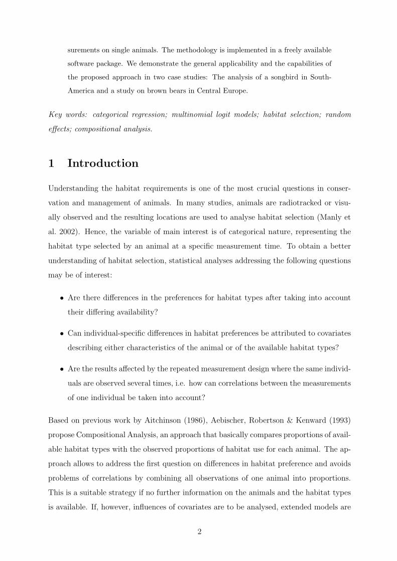
Understanding the habitat requirements is one of the most crucial questions in conser-

vation and management of animals. In many studies, animals are radiotracked or visu-

ally observed and the resulting locations are used to analyse habitat selection (Manly et

al. 2002). Hence, the variable of main interest is of categorical nature, representing the

habitat type selected by an animal at a specific measurement time. To obtain a better

understanding of habitat selection, statistical analyses addressing the following questions

may be of interest:

• Are there differences in the preferences for habitat types after taking into account

their differing availability?

• Can individual-specific differences in habitat preferences be attributed to covariates

describing either characteristics of the animal or of the available habitat types?

• Are the results affected by the repeated measurement design where the same individ-

uals are observed several times, i.e. how can correlations between the measurements

of one individual be taken into account?

Based on previous work by Aitchinson (1986), Aebischer, Robertson & Kenward (1993)

propose Compositional Analysis, an approach that basically compares proportions of avail-

able habitat types with the observed proportions of habitat use for each animal. The ap-

proach allows to address the first question on differences in habitat preference and avoids

problems of correlations by combining all observations of one animal into proportions.

This is a suitable strategy if no further information on the animals and the habitat types

is available. If, however, influences of covariates are to be analysed, extended models are

2

required. In particular, if covariates are changing over the measurement times, a model

based on the original observations seems to be recommended. In Section 4 we will consider

an example on habitat selection of brown bears where animal-specific covariates such as

age or dispersal status and habitat-specific covariates such as exposure to different types

of roads are suspected to influence habitat selection.

Logistic regression uses a dichotomised version of habitat selection as the response vari-

able. This is usually presence/absence of a species, in case of only two habitat types (e.g.

forested versus open areas) it can also be the selection of these habitat types. In case

of presence/absence data, radiolocations are often used as presence data while random

points within the home range or the study area (e.g. Poscillio et al. (2004)) are used as

absence data. There are also examples where the study area is divided into grid cells and

presence/absence data are defined based on cells being inside or outside of homeranges

(e.g. Mladenoff et al. (1995), Schadt et al. (2002)). Keating & Cherry (2004) showed how

logistic regression could be used in case of pseudo-absence data. The advantage of logistic

regression is the possibility to include covariate effects directly, thereby quantifying the

influence of covariates on the habitat selection process. However, logistic regression is

naturally restricted to the analysis of one (in case of presence/absence data) or two habi-

tat types. Separate logistic regressions for the different habitat types can be performed,

but these separate analyses neglect correlations between the habitat selection processes

and may therefore lead to biased estimates for the covariate effects.

Ecological Niche Factor Analysis (ENFA) introduced by Hirzel et al. (2002) implements

an approach based on principal component analysis that avoids the need for absence

data required in logistic regression. Observation points of animals in the ecogeographical

variable (EGV) space defined by the covariates are related to the overall distribution of

these covariates. Concentration of observations in a particular subset of the EGV space

indicates specialisation of the animals and therefore hints at corresponding habitat pref-

erences. These habitat preferences can be visualised, for example, in habitat suitability

maps.

Multinomial logit or discrete choice models, though being rarely used in the context of

habitat selection, allow for the simultaneous analysis of several habitat types, and au-

tomatically take the dependence in the selection processes into account. Like ENFA,

multinomial logit models use only the observed locations as sample units, therefore mak-

3

ing the debate about the proper generation of absence data in logistic regression obsolete.

To our knowledge only three studies have used simple versions of multinomial logit mod-

els in habitat selection studies (Arthur et al. (1996), Cooper & Millspaugh (1999), and

McCracken, Manly & Vander Heyden (1998)). McCracken et al. (1998) give a detailed

introduction into multinomial logit models and discuss a simple example of one black

bear female. However, the authors only define availability globally. So in their case, avail-

ability is only estimated and constant over each year. Arthur et al. (1996) demonstrate

with an example of five female polar bears in the Bering and Chukchi seas how to deal

with changing availability. They defined availability as circles around each location to

account for the highly variable nature of sea ice. Finally, Cooper & Millspaugh (1999)

used multinomial logit models to analyse the selection of 131 day-bed sites by 26 adult

elks in South Dakota, USA. The authors used changing availability and different metric

and categorical covariates. In all three studies repeated observations on the same subject

are treated as independent and therefore intra-individual correlations are neglected.

In the following Section 2, we introduce a general approach for the analysis of habitat

preferences based on an extended version of the multinomial logit model. The general

applicability and flexibility of the approach are demonstrated in two case studies on 33

individuals of a songbird from the coastal rain forest in Brazil (Section 3) and 22 brown

bears from Central Europe (Section 4). Section 5 concludes the paper and comments on

possible extensions.

2 Modelling Habitat Selection

In the following, we present a unifying framework for the analysis of habitat selection

based on a multinomial logit model that combines the following features:

• Availability is measured and can vary for the subunits (e.g. individuals, locations).

An offset term is included in the model to account for availability.

• Both categorical and continuous variables can be included as covariates. Covariates

may vary over time and are allowed to be either habitat-specific or fixed for all

habitat types. In particular, covariates can describe the available habitat types

(such as the average distance to roads or elevation, which dependent on both the

4

habitat category and the time of the measurement) or the animals (such as sex or

age, which are time-constant and time-varying, respectively).

• Individual-specific random effects account for intra-individual correlations.

• The set of available habitat types is allowed to vary, i.e. certain habitat types may

be excluded from the choice set.

• The model in principle supports a number of extensions, such as random slopes or

nonparametric modelling of covariate effects based on penalised splines, see the final

Section 5 for some further remarks.

We start with the multinomial logit model as a basic discrete choice model for our analysis

of habitat selection and assume that there are k different types of habitats. Observations

on n animals are collected at different points in time t. The probability of choosing habitat

type r at time t by animal i is denoted by π(r)it and is related to the covariates via

π(r)it ∝ A

(r)it exp(β(r) + b

(r)i + x′itγ

(r) + z(r)it

′δ) (1)

where ∝ denotes proportionality up to a multiplicative constant. The parameters in model

(1) are defined as follows:

A(r)it : The availability of habitat type r at time t for animal i. This is a known constant,

which is typically proportional to the habitat fraction of the available space. Setting

A(r)it = 0 for some habitat types r allows to exclude these habitat types from the

choice set. In the context of regression models, A(r)it is called an offset and is intro-

duced to account for the varying availability of the habitat types. After inclusion

of the offset, all habitat types virtually have the same size.

β(r) are the parameters of main interest, which indicate the overall habitat preference for

the observed animals after accounting for possible covariate effects and availability.

Positive parameter values indicate a preference for the corresponding habitat type.

b(r)i : To account for correlations between observations on one specific animal i, individual-

specific random effects b(r)i are included. The random effects are assumed to be

independent and identically Gaussian distributed with category-specific variances,

i.e. b(r)i ∼ N(0, τ 2

r ). Introduction of category-specific random effects allows for

5

individual-specific deviations of the selection preferences from the overall pattern

defined by the fixed effects parameters β(r). Defining the expectation of b(r)i to be

zero ensures that β(r) can still be interpreted as the overall selection effect since, on

average, animals follow this pattern.

γ(r) are the parameters corresponding to the effect of covariates xit depending on time

(e. g. daytime of the measurement), and on the animal (e. g. age) but not on the

category.

δ are the parameters corresponding to the effect of covariates z(r)it which are dependent

on the habitat type r (e. g. distance to a road).

Depending on a suitable definition of the covariates, many tools of regression analysis

can be employed for the analysis of habitat suitability and we will demonstrate some

possibilities later-on in the applications.

Since the selection probabilities for the k habitat types have to sum to one, some of

the category-specific parameters in the model specification are redundant. We choose

the last category as reference and define β(k) = b(k)i = γ(r) = 0 to ensure identifiability.

Furthermore, we define A(k)it = 1, i.e. availability is defined relative to the availability

of the reference category. To be able to assess the effect of habitat specific variables

z(r)it , their values also have to be taken relative to the value in the reference category.

Technically the values z(r)it in the reference category are set to zero and in the other

categories z(r)it represents the difference of the variable to the corresponding value for the

reference category. To get a valid model, we furthermore need the assumption that the

reference category is available at all time points t for for all animals i, since otherwise we

can not set A(k)it = 1 and can not define z

(r)it as described above.

After accounting for the identifiability restrictions imposed by the sum-to-one constraint

for the selection probabilities, interpretation of the regression coefficients in the model

is most easily accomplished on the level of ratios of probabilities. For the ratio of the

probabilities for habitat type r compared to the probability for the reference type, we

obtain the expression

π(r)it

π(k)it

= A(r)it exp

(β(r) + b

(r)i + x′itγ

(r) + z(r)it

′δ)

, (2)

6

i.e. model equation (1). Accordingly, covariate effects have to be interpreted multiplica-

tively on ratio of probabilities π(r)it /π

(k)it in (2).

Estimation of all components of the multinomial logit model is based on maximum like-

lihood principles. Inference about model components, e.g. significance tests on some of

the regression coefficients, can be based on the large sample properties of these estimates.

Appendix A summarises inferential procedures and gives further references.

The approach is implemented in the software package BayesX, which is available free of

charge from http://www.stat.uni-muenchen.de/~bayesx.

We discuss other approaches in the context of our approach:

• The model of Arthur et al. (1996) can be seen as special case of our model. There it

is assumed that the availability parameters are constant over time for each animal,

i.e. A(r)i1 = . . . = A

(r)it = . . . = A

(r)iTi

. The parameters β(r) (ωk in their notation) are

the only parameters in their model. They also use maximum likelihood estimation,

which is much easier to handle in the simplified version of our more complex model.

• The methods used by Aitchinson (1986) and Aebischer et al. (1993) are based on a

transformation of the data. Our model can be simply rewritten as

ln π(r)it − ln A

(r)it = (β(r) + b

(r)i + xit

′γ(r) + z(r)it

′δ) + const (3)

Using the reference habitat k this gives

ln(π

(r)it /π

(k)it

)− ln

(A

(r)it /1

)= (β(r) + b

(r)i + xit

′γ(r) + z(r)it

′δ) (4)

The corresponding relative frequencies of the left hand side of (4) are modelled by a

normal distribution. This approximation has been proven to be useful in practice.

The simple model used by Aebischer et al. (1993) is a special case without the

covariates xit, z(r)it . In the general case, one has to assume that the covariates are

constant over time. i.e. xi1 = . . . = xiT and z(r)it1 = . . . = z

(r)iT . So the approach can

be seen as an approximation of our model for the case of fixed further regressors.

7

3 Case Study I: Songbirds

3.1 Data collection

The study area of the songbird example is situated in the Mata Atlantica, the Coastal

Rain Forest in Brazil. From February 2003 through January 2005 a total of 86 individ-

ual Blue Manakins (Chiroxiphia caudata, PIPRIDAE), a small understory omnivorous

bird with about 15cm body length and 25g body mass, were captured and radio-tagged.

During periods of 10 to 47 days – depending on battery life of the transmitter – at least

one location per individual and day was taken. In our analyses, we only used individ-

uals with at least 10 days of radio-tracking data, i.e. 33 different Blue Manakins. All

these individuals lived in a fragmented landscape with woodlots of secundary forest and

agricultural areas and settlements in between. We distinguished between the following

habitat types: agricultural fields, fallow land, human settlements, young to intermediate

forest, old forest and eucalypt plantation. Old forest has been taken to be the reference

category (see Hansbauer (2007) for a detailed description).

3.2 Data Processing

All data were processed in the Geographical Information System (GIS) ArcView 3.1

(ESRI, 1992–1998) and a a Mimimum Convex Polygon (MCP) for each individual was

calculated using Animal Movement 2.0 (Hooge, Eichenlaub & Solomon 1999). This can

be considered as a home range for resident individuals or the area, in which they spent

their time during dispersal. Since it is obvious that the available area for each individual

is bigger than its MCP, each MCP was buffered with the average distance between consec-

utive locations, which was 200m in this example. This area was defined as the available

area for each individual. There might be other ways to define the available areas, e.g.

based on Kernel estimates (two-dimensional density estimates), but this is not the scope

of this paper. Finally, a database was built with the single locations as records and the

percentages of available habitat.

8

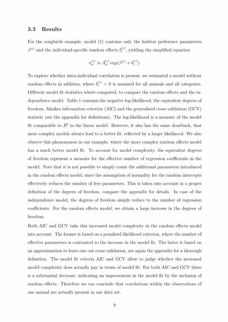
3.3 Results

For the songbirds example, model (1) contains only the habitat preference parameters

β(r) and the individual-specific random effects b(r)i , yielding the simplified equation

π(r)it ∝ A

(r)it exp(β(r) + b

(r)i ).

To explore whether intra-individual correlation is present, we estimated a model without

random effects in addition, where b(r)i = 0 is assumed for all animals and all categories.

Different model fit statistics where computed, to compare the random effects and the in-

dependence model. Table 1 contains the negative log-likelihood, the equivalent degrees of

freedom, Akaikes information criterion (AIC) and the generalised cross validation (GCV)

statistic (see the appendix for definitions). The log-likelihood is a measure of the model

fit comparable to R2 in the linear model. However, it also has the same drawback, that

more complex models always lead to a better fit, reflected by a larger likelihood. We also

observe this phenomenon in our example, where the more complex random effects model

has a much better model fit. To account for model complexity, the equivalent degrees

of freedom represent a measure for the effective number of regression coefficients in the

model. Note that it is not possible to simply count the additional parameters introduced

in the random effects model, since the assumption of normality for the random intercepts

effectively reduces the number of free parameters. This is taken into account in a proper

definition of the degrees of freedom, compare the appendix for details. In case of the

independence model, the degrees of freedom simply reduce to the number of regression

coefficients. For the random effects model, we obtain a large increase in the degrees of

freedom.

Both AIC and GCV take this increased model complexity in the random effects model

into account. The former is based on a penalised likelihood criterion, where the number of

effective parameters is contrasted to the increase in the model fit. The latter is based on

an approximation to leave one out cross validation, see again the appendix for a thorough

definition. The model fit criteria AIC and GCV allow to judge whether the increased

model complexity does actually pay in terms of model fit: For both AIC and GCV there

is a substantial decrease, indicating an improvement in the model fit by the inclusion of

random effects. Therefore we can conclude that correlations within the observations of

one animal are actually present in our data set.

9

−2l df AIC GCV

independence model 2205.7 5 2215.7 1.21

random effects model 1868.5 56.5 1981.5 0.97

Table 1: Model fit criteria in the songbirds example.

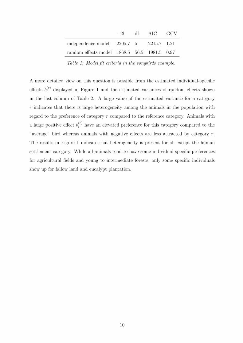
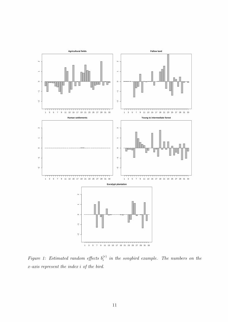
A more detailed view on this question is possible from the estimated individual-specific

effects b(r)i displayed in Figure 1 and the estimated variances of random effects shown

in the last column of Table 2. A large value of the estimated variance for a category

r indicates that there is large heterogeneity among the animals in the population with

regard to the preference of category r compared to the reference category. Animals with

a large positive effect b(r)i have an elevated preference for this category compared to the

”average” bird whereas animals with negative effects are less attracted by category r.

The results in Figure 1 indicate that heterogeneity is present for all except the human

settlement category. While all animals tend to have some individual-specific preferences

for agricultural fields and young to intermediate forests, only some specific individuals

show up for fallow land and eucalypt plantation.

10

1 3 5 7 9 11 13 15 17 19 21 23 25 27 29 31 33

Agricultural fields

−2

−1

01

2

1 3 5 7 9 11 13 15 17 19 21 23 25 27 29 31 33

Fallow land

−2

−1

01

2

1 3 5 7 9 11 13 15 17 19 21 23 25 27 29 31 33

Human settlements

−2

−1

01

2

1 3 5 7 9 11 13 15 17 19 21 23 25 27 29 31 33

Young to intermediate forest−

2−

10

12

1 3 5 7 9 11 13 15 17 19 21 23 25 27 29 31 33

Eucalypt plantation

−2

−1

01

2

Figure 1: Estimated random effects b(r)i in the songbird example. The numbers on the

x-axis represent the index i of the bird.

11

Category β sd 95% CI p-value τ 2r

agricultural fields -3.38 0.361 -4.09 -2.67 <0.0001 1.83

fallow land -1.38 0.365 -2.09 -0.66 0.0003 1.81

human settlements -4.03 0.411 -4.84 -3.23 <0.0001 0.01

young to intermediate forest -0.93 0.244 -1.41 -0.46 0.0003 1.03

eucalypt plantation -2.27 0.421 -3.09 -1.44 <0.0001 1.64

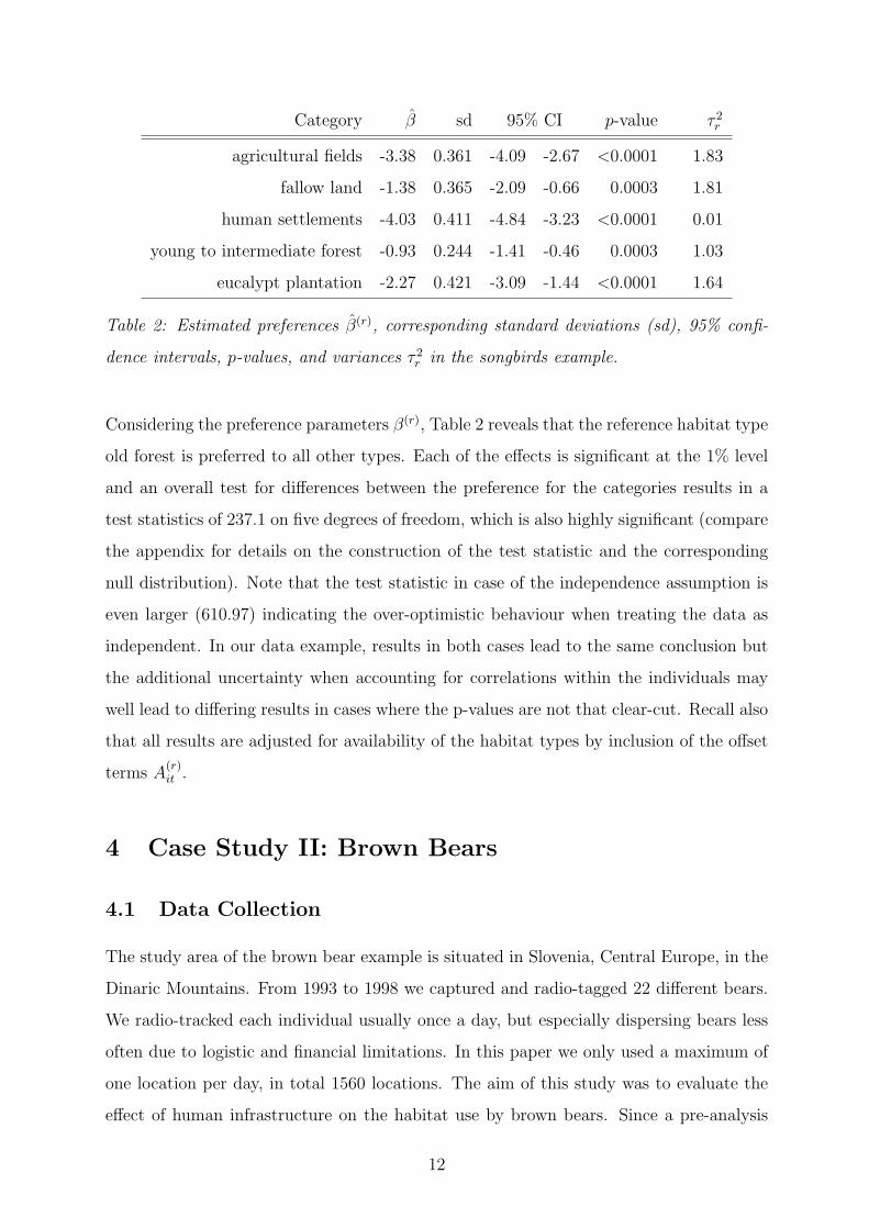
Table 2: Estimated preferences β(r), corresponding standard deviations (sd), 95% confi-

dence intervals, p-values, and variances τ 2r in the songbirds example.

Considering the preference parameters β(r), Table 2 reveals that the reference habitat type

old forest is preferred to all other types. Each of the effects is significant at the 1% level

and an overall test for differences between the preference for the categories results in a

test statistics of 237.1 on five degrees of freedom, which is also highly significant (compare

the appendix for details on the construction of the test statistic and the corresponding

null distribution). Note that the test statistic in case of the independence assumption is

even larger (610.97) indicating the over-optimistic behaviour when treating the data as

independent. In our data example, results in both cases lead to the same conclusion but

the additional uncertainty when accounting for correlations within the individuals may

well lead to differing results in cases where the p-values are not that clear-cut. Recall also

that all results are adjusted for availability of the habitat types by inclusion of the offset

terms A(r)it .

4 Case Study II: Brown Bears

4.1 Data Collection

The study area of the brown bear example is situated in Slovenia, Central Europe, in the

Dinaric Mountains. From 1993 to 1998 we captured and radio-tagged 22 different bears.

We radio-tracked each individual usually once a day, but especially dispersing bears less

often due to logistic and financial limitations. In this paper we only used a maximum of

one location per day, in total 1560 locations. The aim of this study was to evaluate the

effect of human infrastructure on the habitat use by brown bears. Since a pre-analysis

12

showed no difference of open areas and settlements, the two habitat types were combined

into one single habitat type (denoted as ”open areas” for short). For detailed descriptions

see Kaczensky et al. (2003) and Kaczensky et al. (2006).

4.2 Data Processing

For data processing, we proceeded similar as in the songbird example. The average

distance between measured locations has of course to be recomputed and is given by

2500m in our data set. In addition to choice and availability information, two types of

covariates are available:

• bear-specific covariates: age class (yearling, subadult, adult, represented as two

dummy variables in the analyses), sex, and dispersal status (resident or dispersing).

• habitat-specific covariates: elevation, slope, aspect (circular data, represented as the

sum of a sine and a cosine transform in the analyses), and distance to forest roads,

paved roads and to the highway.

For the habitat specific covariates, average values defined based on a grid of random points

(1 point/ha) were used in the following analyses.

Besides a two habitat model with open areas and forested areas as categories, we con-

sidered a second model where forested areas next to roads were defined as additional

habitat types. If the area inside forest is within 1000m to a paved road, then it is ”paved

road”. The areas inside forest and outside ”paved road”, but within 100m to forest roads

describe the habitat type ”forest road”. Other areas inside forest and within 1000m to

the highway are ”highway”. The rest of the forest areas are called ”remote forest”. We

derived the distances to the different road types by visually comparing the frequencies

over the distance of locations with those of random points. In the five-category model we

only used the habitat-specific covariates elevation, slope, and aspect in addition to the

bear-specific covariates as explanatory variables.

4.3 Two habitat types

To select the relevant subset of covariates from the set of possible explanatory variables,

we performed a backward-forward variable selection within the random effects model with

13

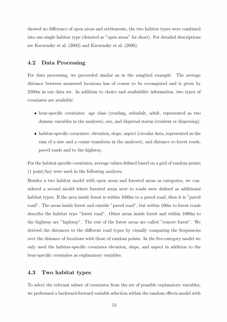
β/δ sd 95% CI p-value τ 2r

open area -2.943 0.476 -3.876 -2.010 <0.0001 0.40

distance to forest road -0.005 0.003 -0.013 0.001 0.1166 –

distance to paved road -0.001 0.000 -0.001 0.000 0.0352 –

Table 3: Estimated preferences β(r), covariate effects δ, corresponding standard deviations

(sd), 95% confidence intervals, p-values, and variance τ 2r in the brown bears example with

two habitat types.

AIC as optimality criterion. Forested areas were treated as the reference category. It turns

out, that only distance to forest roads and distance to paved roads appear as influential

variables in the final model, see Table 3. For the independence model we did not perform

variable selection but re-estimated the model obtained from the random effects model

selection procedure. This makes it easier to compare results from both types of models.

For interpreting estimated effects of habitat-specific covariates, we have to relate the dif-

ference between the covariate value for open areas and the covariate value in forested

areas. For example, for the effect of paved roads, the difference between average distance

to paved roads in open areas and average distance to paved roads in forested areas is

considered as the covariate of interest and multiplied with the estimated regression co-

efficient. In our results this coefficient is negative, indicating that a higher distance in

open areas compared to forested areas further increases the avoidance of open areas. This

unexpected behaviour is, however, supported by bivariate exploratory analyses, where the

average distance to paved roads is substantially smaller for bears choosing open areas as

compared to bears in forested areas. For forest roads, average distances in both habitat

types are comparable in the data set. Note also, that both effects are not significant at

the 1% level and, as a consequence, no definite conclusion about the effect of distance to

roads can be drawn.

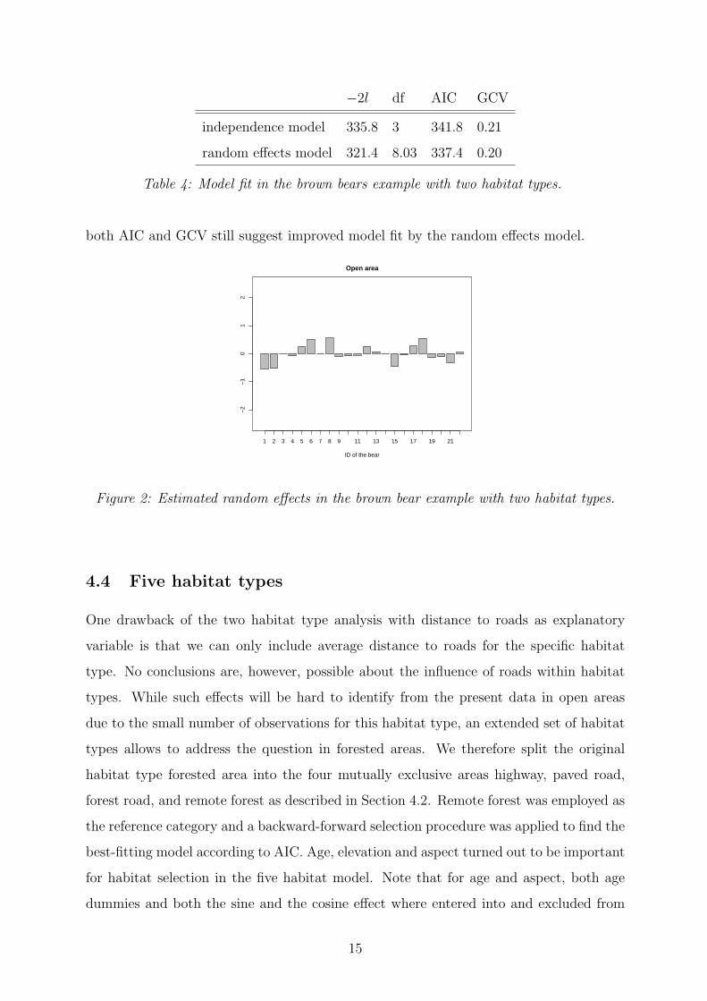
Significant differences between habitat preferences for the two habitat types are identified

in both the independence and the random effects model with a clear favor of forested areas

compared to open areas. The differences between the random effects and the independence

model are smaller than for the bird data, as indicated both by the estimated regression

coefficients and the magnitude of estimated individual-specific effects (Figure 2). However,

14

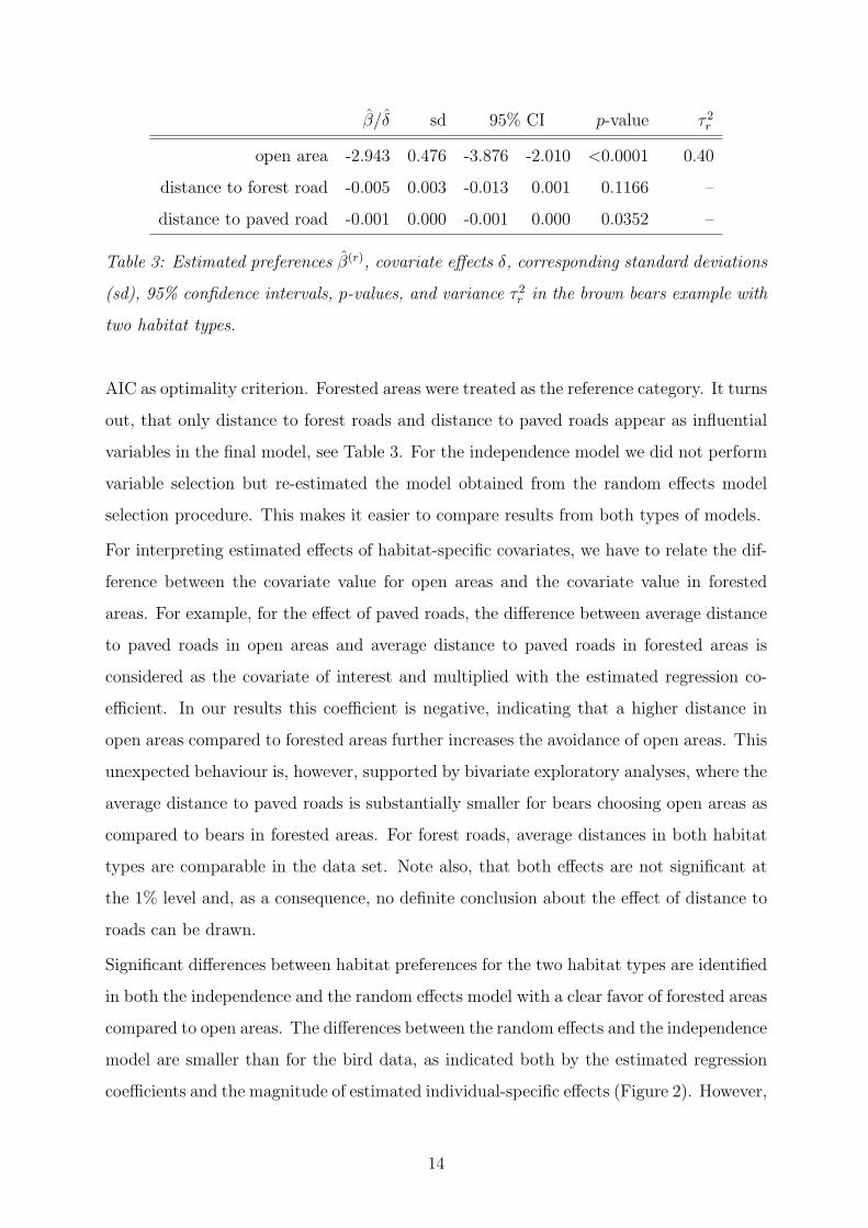
−2l df AIC GCV

independence model 335.8 3 341.8 0.21

random effects model 321.4 8.03 337.4 0.20

Table 4: Model fit in the brown bears example with two habitat types.

both AIC and GCV still suggest improved model fit by the random effects model.

1 2 3 4 5 6 7 8 9 11 13 15 17 19 21

Open area

ID of the bear

−2

−1

01

2

Figure 2: Estimated random effects in the brown bear example with two habitat types.

4.4 Five habitat types

One drawback of the two habitat type analysis with distance to roads as explanatory

variable is that we can only include average distance to roads for the specific habitat

type. No conclusions are, however, possible about the influence of roads within habitat

types. While such effects will be hard to identify from the present data in open areas

due to the small number of observations for this habitat type, an extended set of habitat

types allows to address the question in forested areas. We therefore split the original

habitat type forested area into the four mutually exclusive areas highway, paved road,

forest road, and remote forest as described in Section 4.2. Remote forest was employed as

the reference category and a backward-forward selection procedure was applied to find the

best-fitting model according to AIC. Age, elevation and aspect turned out to be important

for habitat selection in the five habitat model. Note that for age and aspect, both age

dummies and both the sine and the cosine effect where entered into and excluded from

15

the model simultaneously.

Tables 5 and 6 summarise the estimated preferences and covariate effects. For both year-

lings and adults, significant differences in habitat preference are found in the data. In

contrast, differences for subadults are not significant and the corresponding estimates

have relatively large standard deviations. When re-estimating the model without random

effects, these standard deviations are dramatically reduced, leading to the false conclu-

sion, that also for subadults significant differences could be found. Note, that the point

estimates vary to quite some extent between the random effects and the independence

model. This is most clearly observed for the highway preference parameter of subadults

that changes from a large (and significant) positive value in the independence model to

a slightly negative (and insignificant) value in the random effects model. Such dramatic

changes are not typical in random effects models, where mostly the magnitude of point es-

timates remains comparable whereas the standard deviation typically increases. However,

in our example, the increase in the standard deviation is so large, that the corresponding

confidence interval would even contain the value from the independence model.

Similar as in the two habitat analysis, remote forest areas are preferred compared to open

areas. For the forest road habitat type almost no differences to remote forest are found

so that both habitat types are comparable in preference. Results for highways may be

surprising at first sight since our analyses indicate an increased preference compared to

purely forested areas for yearlings and adults (i.e. mostly residential bears). However,

this habitat type is not only characterised by the presence of noise but also by an almost

total absence of human intervention. This seems to attract yearlings and adults whereas

subadults rate the highway habitat type comparable to open areas. The results for paved

roads are more difficult to interpret but seem to be caused by some interaction between

habitat type and the covariates elevation and aspect. Re-estimating the model without

these covariates shows that now remote forest is preferred over all other habitat types and

that paved roads have a large negative effect (as expected). Obviously, the distribution of

elevation and aspect is not uniform over the habitat types but there is some interaction

that leads to the somewhat unintuitive results. This gives a very clear example on the

importance of carefully checking results for an ecological interpretation, in particular in

small data sets as the one employed in our analyses.

The results in Table 6 indicate a preference for regions with higher elevation. Note

16

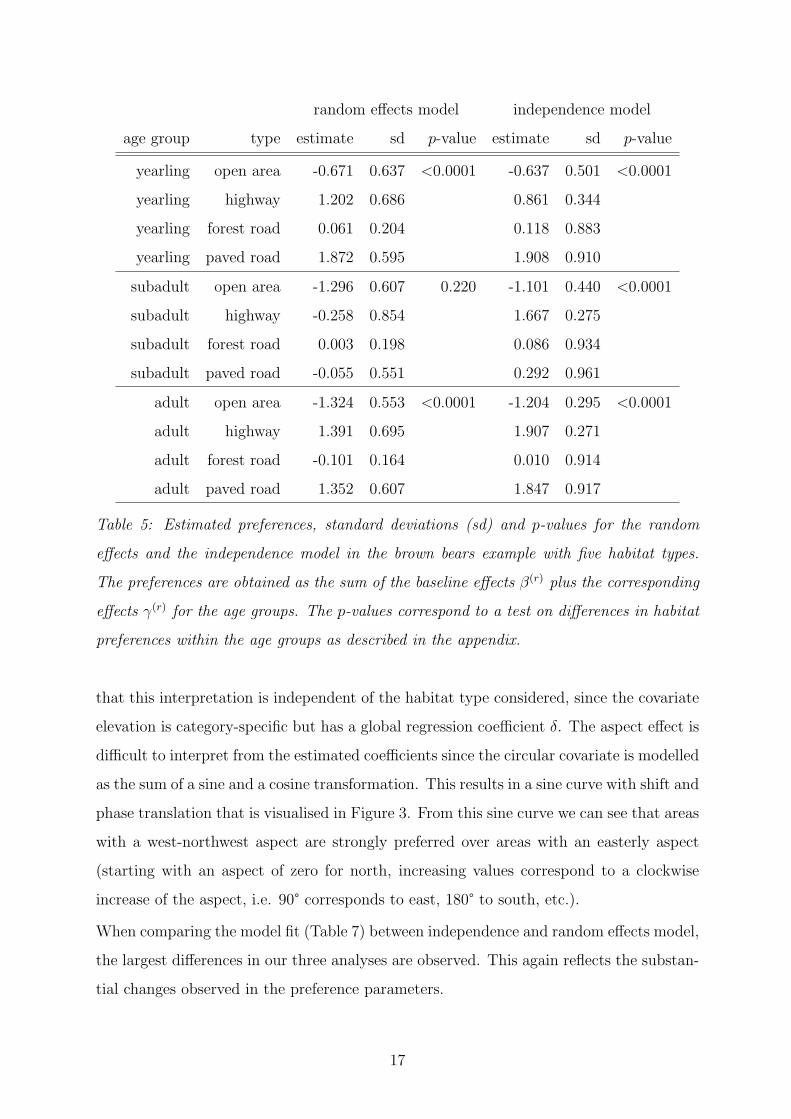
random effects model independence model

age group type estimate sd p-value estimate sd p-value

yearling open area -0.671 0.637 <0.0001 -0.637 0.501 <0.0001

yearling highway 1.202 0.686 0.861 0.344

yearling forest road 0.061 0.204 0.118 0.883

yearling paved road 1.872 0.595 1.908 0.910

subadult open area -1.296 0.607 0.220 -1.101 0.440 <0.0001

subadult highway -0.258 0.854 1.667 0.275

subadult forest road 0.003 0.198 0.086 0.934

subadult paved road -0.055 0.551 0.292 0.961

adult open area -1.324 0.553 <0.0001 -1.204 0.295 <0.0001

adult highway 1.391 0.695 1.907 0.271

adult forest road -0.101 0.164 0.010 0.914

adult paved road 1.352 0.607 1.847 0.917

Table 5: Estimated preferences, standard deviations (sd) and p-values for the random

effects and the independence model in the brown bears example with five habitat types.

The preferences are obtained as the sum of the baseline effects β(r) plus the corresponding

effects γ(r) for the age groups. The p-values correspond to a test on differences in habitat

preferences within the age groups as described in the appendix.

that this interpretation is independent of the habitat type considered, since the covariate

elevation is category-specific but has a global regression coefficient δ. The aspect effect is

difficult to interpret from the estimated coefficients since the circular covariate is modelled

as the sum of a sine and a cosine transformation. This results in a sine curve with shift and

phase translation that is visualised in Figure 3. From this sine curve we can see that areas

with a west-northwest aspect are strongly preferred over areas with an easterly aspect

(starting with an aspect of zero for north, increasing values correspond to a clockwise

increase of the aspect, i.e. 90° corresponds to east, 180° to south, etc.).

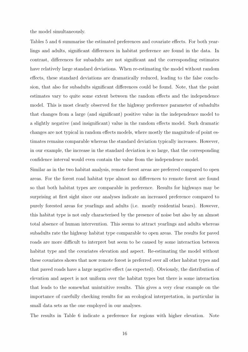
When comparing the model fit (Table 7) between independence and random effects model,

the largest differences in our three analyses are observed. This again reflects the substan-

tial changes observed in the preference parameters.

17

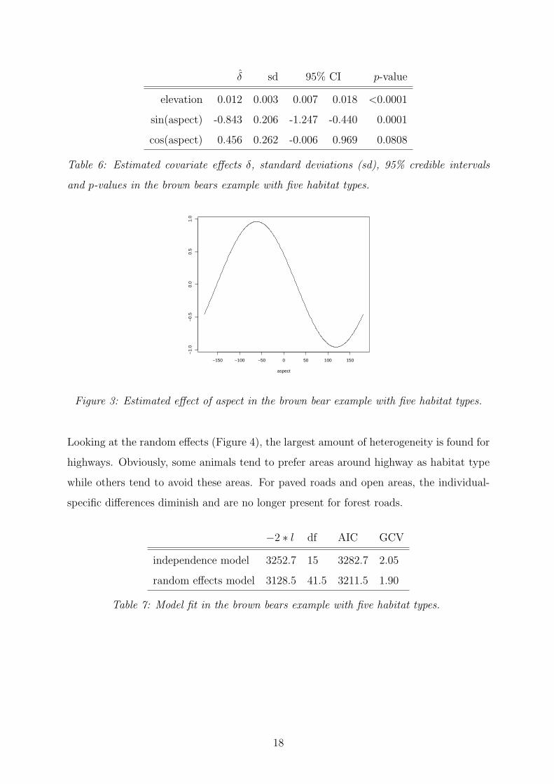
δ sd 95% CI p-value

elevation 0.012 0.003 0.007 0.018 <0.0001

sin(aspect) -0.843 0.206 -1.247 -0.440 0.0001

cos(aspect) 0.456 0.262 -0.006 0.969 0.0808

Table 6: Estimated covariate effects δ, standard deviations (sd), 95% credible intervals

and p-values in the brown bears example with five habitat types.

−150 −100 −50 0 50 100 150

−1.

0−

0.5

0.0

0.5

1.0

aspect

Figure 3: Estimated effect of aspect in the brown bear example with five habitat types.

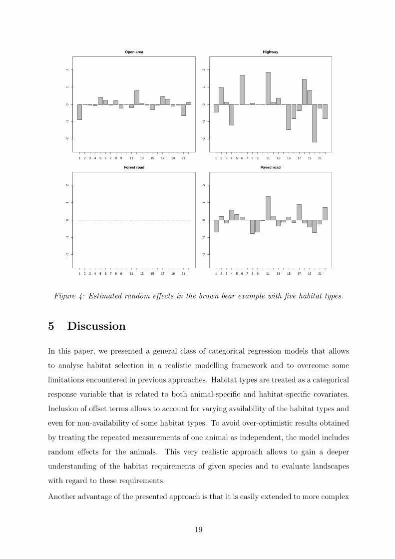
Looking at the random effects (Figure 4), the largest amount of heterogeneity is found for

highways. Obviously, some animals tend to prefer areas around highway as habitat type

while others tend to avoid these areas. For paved roads and open areas, the individual-

specific differences diminish and are no longer present for forest roads.

−2 ∗ l df AIC GCV

independence model 3252.7 15 3282.7 2.05

random effects model 3128.5 41.5 3211.5 1.90

Table 7: Model fit in the brown bears example with five habitat types.

18

1 2 3 4 5 6 7 8 9 11 13 15 17 19 21

Open area

−2

−1

01

2

1 2 3 4 5 6 7 8 9 11 13 15 17 19 21

Highway

−2

−1

01

2

1 2 3 4 5 6 7 8 9 11 13 15 17 19 21

Forest road

−2

−1

01

2

1 2 3 4 5 6 7 8 9 11 13 15 17 19 21

Paved road

−2

−1

01

2

Figure 4: Estimated random effects in the brown bear example with five habitat types.

5 Discussion

In this paper, we presented a general class of categorical regression models that allows

to analyse habitat selection in a realistic modelling framework and to overcome some

limitations encountered in previous approaches. Habitat types are treated as a categorical

response variable that is related to both animal-specific and habitat-specific covariates.

Inclusion of offset terms allows to account for varying availability of the habitat types and

even for non-availability of some habitat types. To avoid over-optimistic results obtained

by treating the repeated measurements of one animal as independent, the model includes

random effects for the animals. This very realistic approach allows to gain a deeper

understanding of the habitat requirements of given species and to evaluate landscapes

with regard to these requirements.

Another advantage of the presented approach is that it is easily extended to more complex

19

situations if needed. For example, we can not only include individual-specific (random)

intercepts but also animal-specific covariate effects, e.g.

π(r)it ∝ A

(r)it exp(β(r) + b

(r)i + x′itγ

(r) + x′itγ(r)i + z

(r)it

′δ),

where γ(r)i denotes the individual-specific deviation from the population parameters γ(r).

Similarly, individual-specific departures can be modeled for the parameter δ or only some

of the covariates can be assumed to have individual-specific effects. In our analyses, we did

not consider such extensions since only a relatively limited number of animals is available.

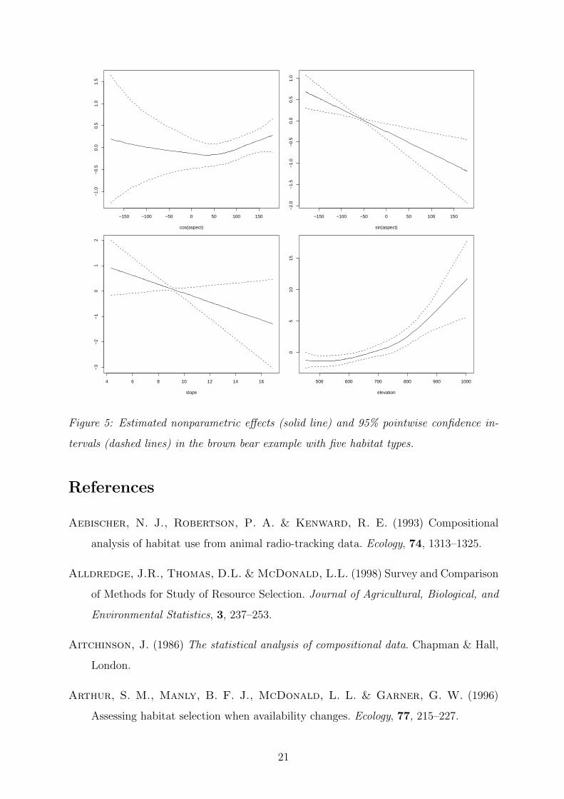
Another extension that greatly extends the flexibility of the presented regression models

are nonparametric effects for some of the continuous covariates. For categorical responses,

such extensions based on penalised splines are described in Kneib & Fahrmeir (2006) and

Kneib, Baumgartner & Steiner (2007). The general idea is to replace the usual linear effect

of a covariate xγ with a flexible yet smooth function f(x). For example, in the brown

bear example with five habitat types, the effects of the aspect transformations, of slope

and of elevation could be included nonparametrically to allow for possible deviations from

a linear covariate effect. For illustration purposes, we estimated such a model with results

shown in Figure 5. For the cosine transformation and elevation we observe some slightly

nonlinear effects, whereas the sine transform as well as the slope effect remain linear. This

already demonstrates one of the advantages of the nonparametric extensions: They allow

for additional flexibility where needed but also suggest linearity of some covariate effects

leading to possible simplifications of the nonparametric model. Note that nonparametric

effects can of course also be included for animal-specific covariates.

In summary, the flexibility and extensibility of the proposed modelling framework for

habitat selection analyses makes it suitable not only for the presented case studies but

also for larger data sets with more complex structures. Embedding the habitat selection

process into a statistical model provides us with well-known measures of the model fit

and possibilities for model validation.

Acknowledgement: We thank Miriam Hansbauer for kindly providing the songbird data

and Stefan Pilz for computational assistance in first analyses of this dataset . The work

of Thomas Kneib and Helmut Kuchenhoff has been supported by the German Science

Foundation, Collaborative Research Center 386 ”Analysis of Discrete Structures”.

20

−150 −100 −50 0 50 100 150

−1.

0−

0.5

0.0

0.5

1.0

1.5

cos(aspect)

−150 −100 −50 0 50 100 150

−2.

0−

1.5

−1.

0−

0.5

0.0

0.5

1.0

sin(aspect)

4 6 8 10 12 14 16

−3

−2

−1

01

2

slope

500 600 700 800 900 1000

05

1015

elevation

Figure 5: Estimated nonparametric effects (solid line) and 95% pointwise confidence in-

tervals (dashed lines) in the brown bear example with five habitat types.

References

Aebischer, N. J., Robertson, P. A. & Kenward, R. E. (1993) Compositional

analysis of habitat use from animal radio-tracking data. Ecology, 74, 1313–1325.

Alldredge, J.R., Thomas, D.L. & McDonald, L.L. (1998) Survey and Comparison

of Methods for Study of Resource Selection. Journal of Agricultural, Biological, and

Environmental Statistics, 3, 237–253.

Aitchinson, J. (1986) The statistical analysis of compositional data. Chapman & Hall,

London.

Arthur, S. M., Manly, B. F. J., McDonald, L. L. & Garner, G. W. (1996)

Assessing habitat selection when availability changes. Ecology, 77, 215–227.

21

Cooper, A. B. & Millspaugh, J. J. (1999) The application of discrete choice models

to wildlife resource selection studies. Ecology, 80, 566–575.

Fahrmeir, L. & Tutz, G. (2001) Multivariate Statistical Modelling based on General-

ized Linear Models. Springer, New York.

Hansbauer, M. M. (2007) Responses of Forest Understory Passerines to Fragmented

Landscapes in the Atlantic Rainforest, South-Eastern Brazil. PhD Thesis, University

of Freiburg.

Hirzel, A. H., Hausser, J., Chessel, D. & Perrin, N. (2002) Ecological niche-

factor analysis: How to compute habitat-suitability maps without absence data?.

Ecology, 83, 2027–2036.

Hooge, P. N., W. Eichenlaub, and E. Solomon (1999) The animal movement

program. USGS, Alaska Biological Science Center.

Kaczensky, P., Huber, D., Knauer, F., Roth, H., Wagner, A. & Kusak, J.

(2006) Activity patterns of brown bears in Slovenia and Croatia. Journal of Zoology,

269, 474–485.

Kaczensky, P., Knauer, F., Krze, B., Jonozovic, M., Adamic, M. & Gossow,

H. (2003) The impact of high speed, high volume traffic axes on brown bears in

Slovenia. Biological Conservation, 111, 191–204.

Keating, K. A. & Cherry, S. (2004) Use and interpretation of logistic regression in

habitat-selection studies. Journal of Wildlife Management, 68, 774-789.

Kneib, T. & Fahrmeir, L. (2006) Structured additive regression for categorical space-

time data: A mixed model approach. Biometrics, 62, 109–118.

Kneib, T., Baumgartner, B. & Steiner, W. J. (2007) Semiparametric Multino-

mial Logit Models for Analysing Consumer Choice Behaviour. AStA Advances in

Statistical Analysis, to appear.

Manly, B. F. J., McDonald, L. L., Thomas, D. L. & Erickson, W. P. (2002)

Resource selection by animals. Kluwer, Doodrecht.

22

McCracken, M. L., Manly, B. F. J. & Vander Heyden, M. (1998) The use

of discrete-choice models for evaluation resource selection. Journal of Agricultural,

Biological, and Environmental Statistics, 3, 268–279.

Mladenoff D.J., Sickley, T.A., Haight,R.G. & Wydeven, A.P. (1995) Regional

Landscape Analysis and Prediction of Favorable Gray Wolf Habitat in the Northern

Great Lakes Region. Conservation Biology, 9, 279-294.

Posillico, M., Meriggi, A., Pagnin, E., Lovari, S. & Russo, L. (2004) A habitat

model for brown bear conservation and land use planning in the central Apennines.

Biological Conservation, 118, 141-150.

Schadt, S., Revilla, E., Wiegand, T., Knauer, F., Kaczensky, P., Breiten-

moser, U., Bufka, L., Cerveny, J., Koubek, P., Huber, T., Stanisa, C. &

Trepl, L. (2002) Assessing the suitability of central European landscapes for the

reintroduction of Eurasian lynx. Journal of Applied Ecology, 39, 189-203.

A Appendix: Inference in multinomial logit models

with random effects

The multinomial logit model discussed in the Section 2 constitutes a multinomial distri-

bution for each of the individual observations yit = (y(1)it , . . . , y

(k)it )′, i.e.

yit ∼ Mu(1, πit),

where πit = (π(1)it , . . . , π

(k)it )′. Hence, the log-likelihood contribution of each of the obser-

vations corresponds to the log-density of such a multinomial distribution and is therefore

given by

lit =k∑

r=1

y(r)it log(π

(r)it ). (5)

Note that in fact the likelihood only depends on the first q = k − 1 probabilities due to

the unit sum constraint. In our approach we automatically account for this due to the

constraints discussed in Section 2.

Under the assumption of independent observations, the joint likelihood would simply be

constructed as the sum of all individual contributions, but since we are considering re-

peated measurements of an individual animal i, the assumption of independence is at least

23

questionable. To account for intra-observational correlations, we introduced individual-

specific random effects in (1) and, as a consequence, the likelihood now consists of two

parts: The conditional distribution of the responses given the random effects and the

random effects distribution. While the former is still of the multinomial form (5) with the

random intercept augmented to the model equation as in (1), the latter expresses the fact

that the sample of analyzed animals is only a random sample from the overall population.

In the following, we consider Gaussian distributed random effects, i.e.

b(r)i i.i.d. N(0, τ 2

r ), i = 1, . . . , n. (6)

which is the most common choice in regression models with random effects and reflects the

assumption that the factors introducing heterogeneity between the animals are approx-

imately Gaussian distributed in the population. Note that the variances of the random

effects depend on the category index r, so that different distributions are utilized for the

choice probabilities of different categories.

To obtain a compact representation of the log-likelihood and further quantities involved

in the estimation process, it is convenient to reexpress the distributional assumption (6)

in multivariate form as

b ∼ N(0, Λ), (7)

where b = (b(1)1 , . . . , b

(1)n , . . . , b

(q)1 , . . . , b

(q)n ), Λ = blockdiag(τ 2

1 In, . . . , τ2q In), and In denotes

the n-dimensional identity matrix. If we analogously define β = (β(1), . . . , β(q))′ and

γ = (γ(1)′ , . . . , γ(q)′)′, this leads to the mixed model log-likelihood

l(β, b, γ, δ) =n∑

i=1

Ti∑t=1

lit − 1

2b′Λ−1b, (8)

where the first term corresponds to the likelihood contributions of the (conditionally

independent) individual measurements and the second term is derived from the multi-

variate Gaussian distribution (7). Equation (8) also has an interesting interpretation as

a penalised log-likelihood: Since a large number of parameters is employed to model the

individual-specific preferences via random effects, some kind of regularisation is needed

to avoid overfitting and to ensure identifiability even in sparse data situations. Both is

introduced by the log-density of the random effect, which essentially can be rewritten as

b′Λ−1b =n∑

i=1

k∑r=1

1

τ 2r

(b(r)i )2 (9)

24

and is therefore simply a sum of squared effects weighted by the corresponding variances.

Hence, (9) acts as a penalty term that penalizes large deviations from the expectation of

the random effects distributions, i.e. deviations from zero. As a consequence, maximum

likelihood estimates for individual-specific effects derived from (8) can be interpreted as a

compromise between fidelity to the data and the prior knowledge expressed through the

random effects distribution.

To actually compute the ML-estimates for both fixed and random effects, we utilized

a Fisher-Scoring algorithm. Let θ = (β′, b′, γ′, δ′)′ denote the vector of all regression

coefficients in the model and let s(θ) and F (θ) be the first and second derivative of (8)

with respect to θ. then the Fisher-scoring algorithm proceeds by iteratively updating the

current estimates via

θ(k+1) = θ(k) + (F (k))−1s(k), (10)

beginning with some starting values θ(0) (compare Kneib & Fahrmeir (2006) for details).

Upon convergence, the Fisher information matrix F (θ) also provides us with the quantities

required for the construction of tests and credible intervals for the regression coefficients.

Asymptotically, with both the number of observations and the replications per individ-

ual large, the ML-estimates are approximately Gaussian distributed and the asymptotic

covariance matrix is given by F−1(θ). For example, we might test the null-hypothesis of

no habitat preference formally via

H0 : β(1) = . . . = β(k−1) = 0 vs. H1 : β(j)0 6= β

(j′)0 for some j 6= j′. (11)

Note that the null hypothesis is in fact equivalent to β(1) = . . . = β(k) = 0 since we

initially assumed β(k) = 0 for identification purposes. The test (11) can be represented in

terms of a general linear hypothesis H0 : Cθ = d vs. H1 : Cθ 6= d, where C is a full rank

matrix. For the particular test (11), we have

C =

1 0 . . . 0

0 1 0...

.... . . . . . . . .

...

0 . . . 0 1 0 . . . 0

and d = (0, . . . , 0). For a general linear hypothesis the score test statistic is given by

(Cθ − d)′(CF (θ)−1C ′)−1(Cθ − d),

25

and is approximately χ2-distributed with rank(C) degrees of freedom, i.e. χ2k−1 in our

example. In Sections 3 and 4 we used this test to assess the presence of habitat preferences.

The last remaining part in the estimation process is the determination of the variance

parameters defining the random effects distributions. In the context of mixed models it is

common praxis not to estimate these quantities from the joint likelihood of θ and Λ but

to use the marginal likelihood for the variance parameters instead, i.e.

Lmarg(Λ) =

∫L(θ, Λ)dθ → max

Λ, (12)

where L(θ, Λ) denotes the multinomial likelihood of the model. In Gaussian mixed models

these estimates are equivalent to the well-known restricted maximum likelihood (REML)

estimates and could be shown to have smaller bias than ordinary ML-estimates derived

from the joint likelihood. In non-Gaussian models it is not as clear whether marginal

likelihood estimates actually perform better than ML-estimates but marginal likelihood

estimation also has a nice Bayesian interpretation which makes them advisable. Pro-

ceeding as in marginal likelihood estimation corresponds to an empirical Bayes procedure

where the variance components are treated as unknown constant hyperparameters to be

estimated from the data. In contrast, the regression coefficients are considered as random

variables and appropriate priors are assigned to them. In the context of mixed models

these are flat priors p(β) ∝ const , p(γ) ∝ const and p(δ) ∝ const for the regression co-

efficients and distribution (7) for the random effects b. In an empirical Bayes approach,

hyperparameters are to be estimated from the marginal predictive density, which (up to

proportionality) coincides with the marginal likelihood (12).

Maximization of (12) can again be carried out using a Fisher-scoring type algorithm.

First and second derivatives can be derived based on rules for matrix differentiation but

we will not discuss this in detail here. A complete description of inferential details in

multinomial logit models with geoadditive predictor and random effects can be found in

Kneib & Fahrmeir (2006).

Goodness of fit measures for the multinomial logit model can be defined in terms of the

deviance residuals

Dit = D(yit, πit) = 2(lit(yit)− lit(πit)),

where lit(·) is the log-likelihood of observation i at time t evaluated for either the obser-

vation itself or the probabilities πit predicted from the current model. The sum of all

26

deviance residuals is called the deviance

D =n∑

i=1

Ti∑t=1

Dit = 2

(n∑

i=1

Ti∑t=1

lit(yit)−n∑

i=1

Ti∑t=1

lit(πit)

)

and based on the deviance and the equivalent degrees of freedom df (see below) we can

define the generalised cross validation criterion

GCV =n

(n− df)2D(y, π)

that allows to compare the performance of different models. In Gaussian linear models,

the above construction leads to the exact leave one out cross validation statistic whereas

in more general models it can be interpreted as an approximation to this quantity.

The degrees of freedom df associated with a model is given by the trace of the hat

matrix projecting the observed responses on their predicted values (see Fahrmeir & Tutz

(2001) for details. Again this definition is motivated from Gaussian linear models where

this definition results exactly in the number of regression coefficients in the model. In

models including random effects, the degrees of freedom is a compromise between the

number of fixed regression coefficients without the random effects and the total number

of parameters. The exact value is governed by the magnitude of the random effects

variance. Based on the degrees of freedom, Akaikes information criterion (AIC) is given

by

AIC = −2n∑

i=1

Ti∑t=1

lit + 2 df .

and can be used as an alternative measure to compare competing regression models with

respect to there model fit.

27