Embed Size (px)
Citation preview
Journal of Global Optimization (2021) 80:195–227https://doi.org/10.1007/s10898-020-00984-y
A general branch-and-bound framework for continuousglobal multiobjective optimization
Gabriele Eichfelder1 · Peter Kirst2 · Laura Meng3 ·Oliver Stein3
Received: 20 July 2020 / Accepted: 12 December 2020 / Published online: 19 January 2021© The Author(s) 2021, corrected publication 2021
AbstractCurrent generalizations of the central ideas of single-objective branch-and-bound to themultiobjective setting do not seem to follow their train of thought all the way. The presentpaper complements the various suggestions for generalizations of partial lower bounds andof overall upper bounds by general constructions for overall lower bounds from partial lowerbounds, and by the corresponding termination criteria and node selection steps. In particular,our branch-and-bound concept employs a new enclosure of the set of nondominated pointsby a union of boxes. On this occasion we also suggest a new discarding test based on alinearization technique. We provide a convergence proof for our general branch-and-boundframework and illustrate the results with numerical examples.
Keywords Multiobjective optimization · Nonconvex optimization · Global optimization ·Branch-and-bound algorithm · Enclosure
1 Introduction
In this paper we propose a general solution approach for continuous multiobjective optimiza-tion problems of the form
min f (x) s.t. g(x) ≤ 0, x ∈ X (MOP)
B Oliver [email protected]
Gabriele [email protected]
Peter [email protected]
Laura [email protected]
1 Institute for Mathematics, Technische Universität Ilmenau, Ilmenau, Germany
2 Operations Research and Logistics (ORL), Wageningen University & Research (WUR),Wageningen, The Netherlands
3 Institute of Operations Research (IOR), Karlsruhe Institute of Technology (KIT), Karlsruhe, Germany
123
196 Journal of Global Optimization (2021) 80:195–227
with a vector f : Rn → R
m of continuous objective functions, a vector g : Rn → R
k
of continuous inequality constraint functions, and an n-dimensional box X = [x, x] withx, x ∈ R
n , x ≤ x . We do not impose any convexity assumptions on the entries of f or g sothat, in particular, the set of feasible points
M = {x ∈ X | g(x) ≤ 0} (1)
is not necessarily convex. Nevertheless, the proposed approach will aim at the global solutionofMOP, in a sense defined below.
The literature on deterministic algorithms for globally solving problems of the typeMOPcan be divided into two classes. One class comprises methods which use a parametric scalar-ization approach and then apply a single objective global optimization technique, mostlybranch-and-bound, to the resulting auxiliary problems for each parameter. Examples and adiscussion of the drawbacks of such approaches are given in [26].
The present paper falls into the second class of solution approaches which try to adapt theideas of single objective branch-and-bound methods directly to the multiobjective setting,that is, they do without the intermediate step of some scalarization approach. The basic ideaof any branch-and-bound algorithm for the minimization of a single function f over a set Mstarts by subdividing M iteratively into partial sets M ′ and then discarding all sets M ′ whichcannot contain minimal points. The discarding tests rely on partial lower bounds for f on thesets M ′, and from them also an overall lower bound for the globally minimal value of f onM can be computed. In addition, the generation of feasible points during the discarding testsleads to overall upper bounds on the globally minimal value. A standard termination criterionfor such algorithms is that the difference between the current overall upper and lower boundsdrops below some prescribed tolerance. Consequently, the choice of a partial set M ′ which isbranched into smaller sets in the next iteration is typically governed by the aim to reduce thedifference between overall upper and lower bounds. As the partial sets M ′ may be interpretedas nodes of the underlying branch-and-bound tree, the latter step is known as node selection.
The contribution of the present paper is motivated by the fact that current generalizationsof the branch-and-bound idea to the multiobjective setting do not seem to follow this trainof thought all the way. In fact, while several suggestions for generalizations of partial lowerbounds and of overall upper bounds are available, we are not aware of general constructionsfor overall lower bounds from partial lower bounds, and of the corresponding terminationcriteria and node selection steps. The aim of the present paper is to close this gap.
In particular, in Sect. 2 we will discuss in more detail that the single objective branch-and-bound idea focuses on constructions in the image space of the optimization problem, whereassome of the known multiobjective branch-and-bound methods invest additional effort intoconstructions in the decision space. While this may be useful for good approximations of theefficient set (to be defined below), it is unrelated to the basic branch-and-bound idea.
The first multiobjective branch-and-bound approach without an intermediate scalarizationstep, but with convergence considerations, was given in [12]. It is formulated for biobjectiveproblems only and focuses on simple discarding tests based on monotonicity considerationsand interval arithmetic. Its node selection rule chooses boxes one by one until all of them aresufficiently small for termination. Branch-and-bound methods for more than two objectivesare proposed in [31] and [11]. The convergence results in [31] rely on growth conditionsof image boxes in terms of decision space boxes as they hold in, e.g., interval arithmetic.The approach from [11] considers general lower bounding procedures for discarding tests,however in combination with a nonstandard notion of ε-efficient sets (to be defined below).Both in [11] and in [31] the termination criterion and node selection rule resemble the onesfrom [12]. In [26] significantly more efficient discarding tests for general multiobjective
123
Journal of Global Optimization (2021) 80:195–227 197
problems on convex feasible sets are suggested, which base on computing partial lowerbounds by convex underestimators of the objective functions instead of interval arithmetic.Their termination criterion is based on a bound for the possible improvement from somelower bounds compared to upper bounds.
A different algorithm for box constrained biobjective problems is presented in [28,37]. Incombination with iterative trisections of the feasible set it makes use of the Lipschitz propertyof the objective functions to compute partial lower bounds via Lipschitz underestimatorsof the objective functions. An overall lower bound is constructed from these partial lowerbounds, and they are compared to some simple overall upper bound in the node selectionrule. However, the generalization of this approach to more objective functions and to moregeneral feasible sets does not seem to be straightforward.
The remainder of this paper is structured as follows. Section 2 reviews some preliminariesfrom single objective branch-and-boundmethods and frommultiobjective optimization. Sec-tion 3 introduces enclosures of the nondominated set ofMOP as well as the computation oftheir widths as the central tools of our approach. Based on the concept of local upper bounds,an explicit choice for an overall upper bounding set within such an enclosure is introduced inSect. 4. The construction of corresponding overall lower bounding sets bases on the partiallower bounding sets used for discarding tests. These are discussed in Sect. 5 along with threeexplicit discarding techniques, where the construction of the corresponding partial lowerbounding sets is based on singletons, convex underestimators and a relaxation-linearizationtechnique, respectively, the latter being novel. Section 6 constructs corresponding overalllower bounding sets from such partial lower bounding sets, before Sect. 7 explicitly states anatural termination criterion, a related node selection rule, and the resulting multiobjectivebranch-and-bound framework in Algorithm 1. Section 8 provides convergence results forthis algorithm, and Sect. 9 complements them with a proof of concept by some numericalillustrations. Section 10 concludes the article with final remarks.
2 Preliminaries
To motivate the concrete branch-and-bound steps in the case of multiobjective optimization,let us first describe the framework for single objective optimization problems in some moredetail.
2.1 Overview of single objective branch-and-bound
In single objective optimization of f overM a globallyminimal point is some xmin ∈ M suchthat no x ∈ M satisfies f (x) < f (xmin) = v, where v denotes the globally minimal value.The discarding tests for subsets M ′ of M are performed by comparing efficiently computablepartial lower bounds �b′ of f on M ′ with the currently best known overall upper bound ub onthe globally minimal value of f on M . The value ub = f (xub) results from the evaluation off at the currently best known feasible point xub ∈ M . In fact, any set M ′ with �b′ > ub maysafely be discarded without deleting a globally minimal point of f on M , since all x ∈ M ′then satisfy f (x) ≥ �b′ > ub ≥ v. Of course also any empty set M ′ can be discarded. Thealgorithm keeps a list L of subsets M ′ which have not yet been discarded.
A branch-and-bound iteration proceeds by choosing and deleting a subset M ′ from L,splitting this subset into two or more parts, and checking if the new subsets may be discardedor if some of them must again be written to L. If during the latter tests a point x ′
ub ∈ M with
123

198 Journal of Global Optimization (2021) 80:195–227
f (x ′ub) < f (xub) is generated, the currently best known feasible point and the corresponding
upper bound are updated to x ′ub and f (x ′
ub), respectively, and possibly further subsets maybe discarded from L by this updated information.
These constructions do not only upper bound the globally minimal value v by ub =f (xub) ≥ v, but they also yield the overall lower bound v ≥ �b := minM ′∈L �b′, sincethe partial minimal values v′ of f on M ′ satisfy v = minM ′∈L v′ and the lower boundingproperty v′ ≥ �b′ thus implies v ≥ �b. Consequently, the minimal value v is sandwichedbetween �b and ub. If for a given tolerance ε > 0 the branch-and-bound method generatesbounds satisfying the termination criterion ub− �b < ε, then, in addition to v ≤ f (xub), thepoint xub also satisfies f (xub) = ub < �b + ε ≤ v + ε and is hence ε-minimal, that is, nox ∈ M satisfies f (x) < f (xub) − ε.
For any ε > 0 the above termination criterion will be met after finitely many branch-and-bound steps if the method chooses points xkub such that ubk = f (xkub) converges to v fromabove, and if for the sets M ′ ∈ Lk the values �bk = minM ′∈Lk �b′ converge to v from below.The latter is usually guaranteed by employing a node selection rule which in the hypotheticalcase ε = 0 would select a set M ′ with �b′ = �bk infinitely often, along with choosing a lowerbounding procedure with appropriate convergence properties.
In practical implementations of such a branch-and-bound framework, the feasible set isusually assumed to be given in the form M = M(X) = {x ∈ X | g(x) ≤ 0} from (1) witha box X . Subdividing M can then be performed by subdividing X into subboxes X ′ andputting M ′ := M(X ′) = {x ∈ X ′ | g(x) ≤ 0}. The list L then only needs to contain theinformation on subboxes X ′ along with their corresponding partial lower bound �b′ for f onM(X ′). A common subdivision step consists in choosing some box X ′ from L and halvingit along a longest edge into two subboxes X1 and X2, which corresponds to splitting the setM ′ = M(X ′) into M1 = M(X1) and M2 = M(X2).
Upon termination of the branch-and-bound method the listLwill contain at least one sub-box X ′ with xub ∈ M(X ′), so that for the entire remaining boxes X ′ inL the set
⋃X ′∈L M(X ′)
as well as its superset⋃
X ′∈L X ′ are nonempty. In addition to the information that xub is ε-minimal, the described construction also implies that both latter sets form coverings of theset of all globally minimal points Xmin of f on M .
This approach, however, neither forces the sizes of the remaining boxes X ′ or of theintervals f (M(X ′)) to become small, nor does it guarantee that the points in the covering⋃
X ′∈L M(X ′) form a subset of the set of ε-minimal points Xεmin . In fact, examples show
that the latter property may not even hold if the termination criterion ub− �b < ε is ignored,but the algorithm terminates after an arbitrary large number of iterations.
Note that, in particular, the single objective branch-and-bound method does not focus ongood approximations ofminimal points xmin , butmainly on the approximation of theminimalvalue v. Moreover, the discarding tests and the termination criteria solely rely on bounds onobjective function values, that is, the approach mainly works in the image set f (M). Belowwe shall see how this carries over to themultiobjective setting. Clearly, working exclusively inthe image space may be algorithmically beneficial since in many multiobjective applicationsits dimension is significantly smaller than the decision space dimension.
2.2 Efficient and nondominated points
In the presence ofmore than one objective function there is in general no feasible point xmin ∈M whichminimizes all objective functions simultaneously, that is, such that f (xmin) ≤ f (x)holds for all x ∈ M . Instead, one takes the equivalent negative formulation of optimality from
123
Journal of Global Optimization (2021) 80:195–227 199
the single objective case, namely, for xmin ∈ M there exists no x ∈ M with f (x) < f (xmin),and transfers it to vector-valued functions f . In fact, a point xwE ∈ M is called weaklyefficient forMOP if there exists no x ∈ M with f (x) < f (xwE ),where the inequality ismeantcomponentwise (cf., e.g., [10,25]). Since in some situations weakly efficient points allow theimprovement of one objective function without any trade-off against other objectives, usuallya stronger concept is employed in which the strict inequality f (x) < f (xmin) from the singleobjective case is rewritten as f (x) ≤ f (xmin) and f (x) �= f (xmin). A feasible point xE ∈ Mis called efficient forMOP if there exists no x ∈ M with f (x) ≤ f (xE ) and f (x) �= f (xE ).The set of all efficient points XE is called efficient set of MOP and forms a subset of theset XwE of all weakly efficient points of MOP. We remark that under our assumptions theproblem MOP possesses efficient points whenever M is nonempty [10]. They usually forma set of infinitely many alternatives from which the decision maker has to choose.
The notion of ε-minimality from the single objective case can be generalized to multi-objective problems as well. For ε > 0 a point xε
E ∈ M is called ε-efficient for MOP (cf.[23] with choice εe ∈ R
m+) if there exists no x ∈ M such that f (x) ≤ f (xεE ) − εe and
f (x) �= f (xεE ) − εe hold, where e stands for the all ones vector. We denote the set of all
ε-efficient points by XεE . It is not hard to see that the chain of inclusions XE ⊆ XwE ⊆ Xε
Eholds for any ε > 0 so that, in particular, under our assumptions all three sets are nonempty.
Whereas efficiency, weak efficiency and ε-efficiency are notions in the decision space Rn ,
as mentioned above the branch-and-bound idea focuses on constructions in the image spaceRm . These are covered by the following concepts. For points y1, y2 ∈ R
m we say that y1
dominates y2 if y1 ≤ y2 and y1 �= y2 holds. In this terminology a point xE ∈ M is efficient ifand only if f (xE ) is not dominated by any f (x) with x ∈ M . Hence, the set YN = f (XE ) ofpoints yN ∈ f (M)which are not dominated by any y ∈ f (M) is called the nondominated set(also known as Pareto set) ofMOP. The nondominated set YN plays the role of the minimalvalue v from the single objective case.
Analogously, theweakly nondominated setYwN = f (XwE ) ofMOP consists of the pointsywN ∈ f (M) such that no y ∈ f (M) satisfies y < ywN , that is, such that no element off (M) strictly dominates ywN , and the ε-nondominated set Y ε
N = f (XεE ) of MOP consists
of the points yεN ∈ f (M) such that no element of f (M) dominates yε
N − εe. In the singleobjective case Y ε
N corresponds to the (rarely discussed) set [v, v + ε] ∩ f (M) of ε-minimalvalues, whereas YwN behaves like YN and collapses to v. In view of our above remarks, thethree sets satisfy YN ⊆ YwN ⊆ Y ε
N for any ε > 0, and they are nonempty for M �= ∅.
3 Enclosing the nondominated set
The first aim of our multiobjective generalization of the branch-and-bound framework is tosandwich the nondominated setYN ofMOP in some sense between an overall lower boundingset LB and an overall upper bounding set UB, where LB is constructed from partial lowerbounding sets. In Sect. 7 this will lead to a termination criterion and a node selection rule.
Since in set notation the single objective sandwiching condition �b ≤ v ≤ ub may berewritten as {v} ⊆ (�b+R+)∩ (ub−R+) (where, e.g., the expression �b+R
m+ is shorthandfor the Minkowski sum {�b} + R
m+), let us generalize it to the requirement
YN ⊆ (LB + Rm+) ∩ (UB − R
m+) (2)
with nonempty and compact sets LB,UB ⊆ Rm . This is in line with the sandwiching
approaches reviewed in [30] which, however, have not been combined with branch-and-bound ideas.
123
200 Journal of Global Optimization (2021) 80:195–227
The enclosing interval [�b, ub] for v from the single objective case thus generalizes to theenclosure
E(LB,UB) := (LB + Rm+) ∩ (UB − R
m+)
for YN . Since the single objective termination criterion ub−�b < ε may be interpreted as anupper bound on the interval length of the enclosing interval [�b, ub], a natural multiobjectivetermination criterion is to upper bound somewidthw(LB,UB) of the enclosure E(LB,UB)
by a tolerance ε. In view of the special structure of the enclosure we suggest to measure itswidth with respect to the direction of the all ones vector e, that is, we define w(LB,UB) asthe supremum of the problem
maxy,t
‖(y + te) − y‖2/√m s.t. t ≥ 0, y, y + te ∈ E(LB,UB). (W (LB,UB))
Thanks to the normalization constant√m the objective function of W (LB,UB) equals t .
Imposing the nonnegativity constraint on t is possible due to symmetry. Lemma 3.3 willprovide a sufficient condition for the solvability of W (LB,UB) which is, however, onlyneeded later. The following lemma first justifies the choice of this width measure.
Lemma 3.1 For sets LB,UB ⊆ Rm with YN ⊆ LB + R
m+ and some ε > 0 letw(LB,UB) < ε. Then the relation
E(LB,UB) ∩ f (M) ⊆ Y εN
holds.
Proof For any y ∈ E(LB,UB) ∩ f (M) assume that there exists some y ∈ f (M) with y ≤y − εe and y �= y − εe. Since our assumptions imply external stability [32, Theorem 3.2.9],the point y either lies in YN or is dominated by some yN ∈ YN . This implies y ∈ YN +R
m+ ⊆LB + R
m+, and together with y ≤ y − εe ≤ y ∈ UB − Rm+ it shows y ∈ E(LB,UB).
Moreover, the point y + εe clearly lies in LB + Rm+, and with y + εe ≤ y ∈ UB − R
m+ wealso obtain y + εe ∈ E(LB,UB). Consequently (y, ε) is a feasible point of W (LB,UB) ,resulting in the contradiction w(LB,UB) ≥ ‖εe‖2/√m = ε. �
Lemma 3.1 states that for w(LB,UB) < ε all attainable points in the enclosureE(LB,UB) are ε-nondominated. In the single objective case (m = 1) this statement col-lapses to the simple observation that for ub−�b < ε all values in the interval [�b, ub]∩ f (M)
are ε-minimal, that is, they lie in [v, v+ε]∩ f (M). Recall that, in combination with discard-ing tests based on ub, this does not entail that the elements of
⋃X ′∈L M(X ′) are ε-minimal
points. Analogously one may not expect that the multiobjective discarding tests based onUB, as discussed in Sect. 5, will yield
⋃X ′∈L M(X ′) ⊆ Xε
E for w(LB,UB) < ε.As the condition y ∈ (LB + R
m+) ∩ (UB − Rm+) is equivalent to the existence of some
�b ∈ LB and ub ∈ UB with �b ≤ y ≤ ub, the enclosure E(LB,UB) can be written as theunion of the nonempty boxes which can be constructed with lower and upper bound vectorsfrom LB and UB, respectively,
E(LB,UB) =⋃
(�b,ub)∈LB×UB�b≤ub
[�b, ub]. (3)
This shows, in particular, that appropriate choices of LB and UB might lead to a discon-nected enclosure E(LB,UB), thus correctly capturing the topological structure of YN .Moreover, the following result relates the computation of w(LB,UB) to the description
123
Journal of Global Optimization (2021) 80:195–227 201
(3) of E(LB,UB) and implies that w(LB,UB) coincides with the largest value s(�b, ub)among the above boxes [�b, ub], where
s(�b, ub) := minj=1,...,m
(ub j − �b j ) (4)
denotes the length of a shortest edge of [�b, ub].Lemma 3.2 For any sets LB,UB ⊆ R
m the width w(LB,UB) of E(LB,UB) coincideswith the supremum of
max�b,ub
s(�b, ub) s.t. (�b, ub) ∈ LB×UB, �b ≤ ub. (W (LB,UB))
Proof Since the objective function of W (LB,UB) satisfies ‖(y + te) − y‖2/√m = t , inparticular it does not depend on y. Hence the supremum of W (LB,UB) coincides with thesupremum of
maxt
t s.t. t ≥ 0, ∃ y ∈ Rm : y, y + te ∈ (LB + R
m+) ∩ (UB − Rm+). (W (LB,UB))
As the condition y ∈ LB+Rm+ implies y+te ∈ LB+R
m+ and, analogously, y+te ∈ UB−Rm+
implies y ∈ UB − Rm+, the latter existence constraint simplifies to
∃ y ∈ Rm : y ∈ LB + R
m+, y + te ∈ UB − Rm+
or, equivalently,
∃ (�b, ub) ∈ LB ×UB : te ≤ ub − �b.
The supremum of W (LB,UB) thus coincides with the supremum of
max�b,ub,t
t s.t. 0 ≤ te ≤ ub − �b, (�b, ub) ∈ LB ×UB
which, after explicitly computing the upper bound s(�b, ub) for t , yields the assertion. �The next result immediately follows from Lemma 3.2 in view of the Weierstrass theorem.
Lemma 3.3 Let the sets LB,UB ⊆ Rm be nonempty and compact, and let E(LB,UB) be
nonempty. Then the problem W (LB,UB) is solvable. In particular, the widthw(LB,UB) isa real number, and there exists some box [�b�, ub�] with (�b�, ub�) ∈ LB ×UB, �b� ≤ ub�
and w(LB,UB) = s(�b�, ub�).
Note that under our assumptions the enclosure E(LB,UB) is nonempty whenever LB andUB satisfy (2), as then ∅ �= YN ⊆ E(LB,UB) holds.
The combination of Lemmas 3.1, 3.2 and 3.3 yields the following explicit sufficientcondition for ε-nondominance of the attainable points in the enclosure E(LB,UB).
Theorem 3.4 For nonempty and compact sets LB,UB ⊆ Rm with (2) and some ε > 0 let
max {s(�b, ub)| (�b, ub) ∈ LB ×UB, �b ≤ ub} < ε. (5)
Then the relation
E(LB,UB) ∩ f (M) ⊆ Y εN
holds.
For the application ofTheorem3.4we shall subsequently construct sequences of nonemptysets (LBk), (UBk) ⊆ R
m with (2) for all k ∈ N as well as limk w(LBk,UBk) = 0. Then,
123
202 Journal of Global Optimization (2021) 80:195–227
in analogy to the single objective case, (5) may be employed as the termination criterion ofa multiobjective branch-and-bound method for any prescribed tolerance ε > 0.
4 Upper bounding the nondominated set
Regarding the generalization of the concept of upper bounds ub = f (xub) for vwith xub ∈ Mfrom the single objective case, observe that the notion of a currently best feasible point doesnot make sense in the multiobjective setting.
4.1 The provisional nondominated set
Instead, different feasible points xub ∈ M may provide good approximations for differentefficient points. Consequently, in the course of the algorithm one keeps a subset Xub of thefinitely many feasible points generated so far or, as we wish to work in the image space, werather keep the setF := f (Xub), whose elements are to approximate different nondominatedpoints ofMOP.
It would be useless, however, to store a point f (x1)with x1 ∈ Xub inF which is dominatedby f (x2) for some x2 ∈ Xub, as in this case the statement that x2 is a better feasible pointthan x1 does make sense. Hence, whenever some new point xub ∈ M is generated in thecourse of the algorithm, its image f (xub) is only inserted into F if f (xub) is not dominatedby any element from F . Moreover, all elements of F which are dominated by f (xub) aredeleted from F . In the following we will refer to this procedure as updating F with respectto f (xub).
The source of the points xub will be elements of subboxes X ′ of X (e.g., their midpointsmid(X ′)) which are chosen for the discarding tests described below. If such an xub ∈ X ′ isfeasible for MOP the list F will be updated with respect to f (xub).
As a consequence of this construction, no element ofF dominates any other element ofF .Any subset of R
m with the latter property is called stable, so that F forms a finite and stablesubset of the image set f (M) of MOP. Observe that also the nondominated set YN of MOPis a (not necessarily finite) stable subset of f (M). This motivates to call F a provisionalnondominated set [12].
From the single objective construction one may expect that the choice UB = F for theupper bounding set in (2) is possible. However, while the inclusion YN ⊆ F∪(F+R
m+)c doeshold, simple examples show that the required inclusion YN ⊆ F − R
m+ may fail. Fortunatelythe following concept, already used in [26], allows us to construct an upper bounding setUBfrom the information in F .
4.2 Local upper bounds
The subsequent construction assumes the existence of a sufficiently large box Z = [z, z]withf (M) ⊆ int(Z) (where int denotes the topological interior). In the present setting of MOPthe set f (M) is contained in the compact set f (X), so that the existence of such a box Zis no restriction. The explicit construction of some suitable Z is possible, for example, byinterval arithmetic, which we shall discuss in more detail in Sect. 5.3.
Given a finite and stable set F ⊆ f (M), the elements of the nondominated set YN can,in particular, not be dominated by any q ∈ F . This motivates to define the so-called search
123
Journal of Global Optimization (2021) 80:195–227 203
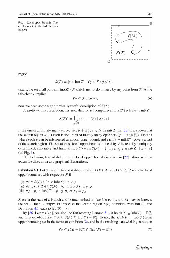
Fig. 1 Local upper bounds. Thecircles mark F , the bullets marklub(F)
f(M)
z
S(F)
z
region
S(F) = {z ∈ int(Z) | ∀q ∈ F : q � z},that is, the set of all points in int(Z)\F which are not dominated by any point fromF . Whilethis clearly implies
YN ⊆ F ∪ S(F), (6)
now we need some algorithmically useful description of S(F).To motivate this description, first note that the set complement of S(F) relative to int(Z),
S(F)c =⋃
q∈F{z ∈ int(Z) | q ≤ z}
is the union of finitely many closed sets q + Rm+, q ∈ F , in int(Z). In [22] it is shown that
the search region S(F) itself is the union of finitely many open sets (p − int(Rm+)) ∩ int(Z)
where each p can be interpreted as a local upper bound, and each p − int(Rm+) covers a partof the search region. The set of these local upper bounds induced by F is actually a uniquelydetermined, nonempty and finite set lub(F) with S(F) = ⋃
p∈lub(F){z ∈ int(Z) | z < p}(cf. Fig. 1).
The following formal definition of local upper bounds is given in [22], along with anextensive discussion and graphical illustrations.
Definition 4.1 Let F be a finite and stable subset of f (M). A set lub(F) ⊆ Z is called localupper bound set with respect to F if
(i) ∀z ∈ S(F) : ∃p ∈ lub(F) : z < p(ii) ∀z ∈ (int(Z)) \ S(F) : ∀p ∈ lub(F) : z ≮ p(iii) ∀p1, p2 ∈ lub(F) : p1 � p2 or p1 = p2
Since at the start of a branch-and-bound method no feasible points x ∈ M may be known,the set F then is empty. In this case the search region S(∅) coincides with int(Z), andDefinition 4.1 leads to lub(∅) = {z}.
By [26, Lemma 3.4], see also the forthcoming Lemma 5.1, it holds F ⊆ lub(F) − Rm+,
and thus we obtain YN ⊆ F ∪ S(F) ⊆ lub(F) − Rm+. Hence, the set UB := lub(F) is an
upper bounding set in the sense of condition (2), and in the resulting sandwiching condition
YN ⊆ (LB + Rm+) ∩ (lub(F) − R
m+) (7)
123
204 Journal of Global Optimization (2021) 80:195–227
it remains to find a suitable lower bounding set LB. We remark that, in the course of abranch-and-bound method, algorithms from [8,22] may be employed to efficiently calculateand update the local upper bound sets lub(F) with respect to the appearing provisionalnondominated sets F .
5 Lower bounding sets for partial upper image sets
Before we turn to the construction of an overall lower bounding set LB which satisfiesthe necessary relation YN ⊆ LB + R
m+ from the sandwiching condition (2), recall that inthe single objective case the overall lower bound �b for the minimal value v is defined as�b = minX ′∈L �b′ with the partial lower bounds �b′ for f on the subsets M(X ′) of M(X). Inaddition to their role in the definition of the overall lower bound �b, the values �b′ are alsoneeded to discard sets M(X ′) with �b′ > ub, since due to minx∈M(X ′) f (x) = v′ ≥ �b′ >
ub ≥ v those sets cannot contain minimal points. To develop a natural generalization of thepartial lower bound �b′ to a partial lower bounding set LB ′ in the multiobjective setting, letus first transfer the latter discarding argument.
5.1 Discarding by partial upper image sets and local upper bounds
Before lower bounding sets are introduced at all, we need a generalization of the fact that aset M(X ′) with minx∈M(X ′) f (x) > ub cannot contain minimal points. In a set formulationthe latter discarding condition can be rewritten as {ub} ∩ ( f (M(X ′)) + R+) = ∅ with thepartial image set f (M(X ′)) of f on M(X ′) and its corresponding partial upper image setf (M(X ′)) + R+. From the discussion on upper bounding sets in Sect. 4.2 one may expectthat the appropriate generalization to the multiobjective setting claims that the condition
lub(F) ∩ (f (M(X ′)) + R
m+) = ∅ (8)
rules out the existence of efficient points in M(X ′), so that X ′ can be discarded from L. Thisis indeed the case. For the proof of the correctness of this discarding condition we need thefollowing two lemmata.
Lemma 5.1 [21,26] Let F be a finite and stable subset of f (M). Then for every q ∈ F andfor every j ∈ {1, ...,m} there is a point p ∈ lub(F) with q j = p j and qk < pk for allk ∈ {1, ...,m} \ { j}.For the present paper the main consequence of Lemma 5.1 is the relation F ⊆ lub(F)−R
m+.
Lemma 5.2 For any subbox X ′ the discarding condition (8) implies
F ∩ (f (M(X ′)) + R
m+) = ∅. (9)
Proof Assume that for some subbox X ′ the condition (9) is violated. Then there exist someq ∈ F and some y ∈ f (M(X ′)) with y ≤ q . Moreover, by Lemma 5.1 there exists a localupper bound p ∈ lub(F)with q ≤ p. This yields y ≤ q ≤ p and, thus, p ∈ f (M(X ′))+R
m+,so that X ′ violates (8) as well. This shows the assertion. �
The main idea of the following result was already presented in [26]. We include its shortproof for completeness.
123
Journal of Global Optimization (2021) 80:195–227 205
Proposition 5.3 Let F be a finite and stable subset of f (M), and let X ′ be a subbox of X.Then (8) implies
YN ∩ (f (M(X ′)) + R
m+) = ∅. (10)
In particular, f (M(X ′)) cannot contain any nondominated point of MOP so that X ′ can bediscarded.
Proof Assume that (8) holds, but some yN ∈ YN lies in f (M(X ′)) + Rm+. Then, on the one
hand, since yN is not dominated by any point in f (M(X)), it must lie in f (M(X ′)). On theother hand, by (6) the point yN either belongs to F or to the search region S(F). The firstcase implies yN ∈ F ∩ f (M(X ′)) which is impossible by Lemma 5.2. In the second case,by Definition 4.1(i) there exists some local upper bound p ∈ lub(F) with p > yN , whichyields p ∈ yN + R
m+ ⊆ f (M(X ′)) + Rm+, in contradiction to (8). This shows (10), of which
the second assertion is an immediate consequence. �Observe that Proposition 5.3 correctly covers also the case of an empty set M(X ′). Also notethat, as in Sect. 4.1, we cannot replace the set lub(F) in (8) byF , since simple examples showthat f (M(X ′)) may contain nondominated points if only the weaker condition (9) holds.
Subsequently we shall need an algorithmically tractable version of at least a sufficientcondition for (8). As a preparation for this as well as for some later developments, for anyz ∈ R
m and a compact set A ⊆ Rm let us consider the auxiliary optimization problem
mint
t s.t. z + te ∈ A + Rm+. (D(z, A))
Its infimum ϕA,e(z) is known as Tammer-Weidner functional [15]. In the present paper wewill abbreviate it by ϕA(z), since we shall exclusively use the direction e. In the case A = ∅the feasible set of D(z, A) is empty, and we follow the usual convention to formally defineϕ∅(z) := +∞. The following two lemmata are based on [7, Proposition 1.41] and [16,Section 2.3].
Lemma 5.4 For any nonempty compact set A ⊆ Rm and z ∈ R
m the feasible set of D(z, A)
possesses the form [ϕ,+∞)with some ϕ ∈ R. In particular, D(z, A) is solvable with optimalpoint as well as optimal value ϕ, and ϕ coincides with ϕA(z).
Lemma 5.5 Let A ⊆ Rm be compact. Then z ∈ A + R
m+ holds if and only if the infimumϕA(z) of D(z, A) satisfies ϕA(z) ≤ 0.
Note that the latter result correctly covers the case A = ∅. The following reformulation ofProposition 5.3 with the help of Lemma 5.5 allows us to check its assumption (8) by solvinga finite number of one-dimensional optimization problems. In fact, the continuity of f and gtogether with the compactness of any subbox X ′ imply the compactness of the partial imageset f (M(X ′)), so that we arrive at the following form of the discarding condition.
Proposition 5.6 Let F be a finite and stable subset of f (M), and let X ′ be a subbox of X. Iffor each p ∈ lub(F) the infimum ϕ f (M(X ′))(p) of
mint
t s.t. p+ te ∈ f (M(X ′))+Rm+ (D(p, f (M(X ′))))
satisfies ϕ f (M(X ′))(p) > 0, then X ′ can be discarded.
Discarding tests basing on Proposition 5.6 may obviously stop to compute the infimaϕ f (M(X ′))(p) of all p ∈ lub(F) as soon as the result ϕ f (M(X ′))(p) ≤ 0 occurs for some p ∈
123
206 Journal of Global Optimization (2021) 80:195–227
lubF , because then the set X ′ cannot be discarded. While in general all values ϕ f (M(X ′))(p),p ∈ lub(F), have to be checked for positivity to guarantee that X ′ may be discarded, in thecaseM(X ′) = ∅ it is of course sufficient to stop these computations afterϕ f (M(X ′))(p) = +∞occurs for the first tested p ∈ lub(F).
We remark that algorithmically the problem D(p, f (M(X ′))) should be treated in itsequivalent lifted formulation
mint,x
t s.t. p + te ≥ f (x), x ∈ M(X ′). (11)
5.2 Discarding by relaxed partial upper image sets and local upper bounds
Unfortunately, for general continuous functions f and g and any p ∈ Rm it may not be
algorithmically tractable to determine the globally minimal value of D(p, f (M(X ′))) or ofits lifted version (11). Instead, sufficient conditions for ϕ f (M(X ′))(p) > 0 can be obtained bychecking the infimum of some tractable relaxation of D(p, f (M(X ′))) for positivity.
A natural approach to the construction of such a relaxation first returns to the generalcondition (8) which we had seen to generalize the requirement ub < minx∈M(X ′) f (x) fromthe single objective case. Also there, in general it is not algorithmically tractable to determinethe value minx∈M(X ′) f (x) so that, instead, for an efficiently computable lower bound �b′ ofminx∈M(X ′) f (x) one only checks the sufficient condition ub < �b′.
In analogy to this, in the multiobjective case we try to find a compact set LB ′ ⊆ Rm with
f (M(X ′))+Rm+ ⊆ LB ′ +R
m+ and such that LB ′ +Rm+ possesses, for example, a polyhedral
or convex smooth description. Then for any p ∈ Rm the condition p /∈ f (M(X ′)) + R
m+ is aconsequence of p /∈ LB ′ + R
m+. Hence, in a branch-and-bound framework any such set LB ′plays the role of a partial lower bound �b′ from the single objective case, which motivatesthe following definition.
Definition 5.7 Let X ′ be a subbox of X . Then any compact set LB ′ ⊆ Rm with f (M(X ′))+
Rm+ ⊆ LB ′ + R
m+ is called partial lower bounding set for f (M(X ′)).
In fact, Proposition 5.3 immediately implies the following discarding test.
Proposition 5.8 Let F be a finite and stable subset of f (M), let X ′ be a subbox of X, andlet LB ′ be some partial lower bounding set for f (M(X ′)). If
lub(F) ∩ (LB ′ + R
m+) = ∅ (12)
holds, then X ′ can be discarded.
By Lemma 5.5 and due to the assumed tractable structure of LB ′, the condition (12) canbe checked efficiently via the positivity of the infima ϕLB′(p) of
mint
t s.t. p+ te ∈ LB ′ +Rm+ (D(p, LB ′))
for all p ∈ lub(F). The following tractable discarding test hence follows fromProposition 5.8.
Theorem 5.9 (General discarding test) Let F be a finite and stable subset of f (M), let X ′ bea subbox of X, and let LB ′ be some partial lower bounding set for f (M(X ′)). If ϕLB′(p) > 0holds for all p ∈ lub(F), then X ′ can be discarded.
As mentioned before, whenever a discarding test for X ′ based on Proposition 5.8 orTheorem 5.9 fails, we may at least check whether some point x ′ ∈ X ′ lies in M(X ′). If this
123
Journal of Global Optimization (2021) 80:195–227 207
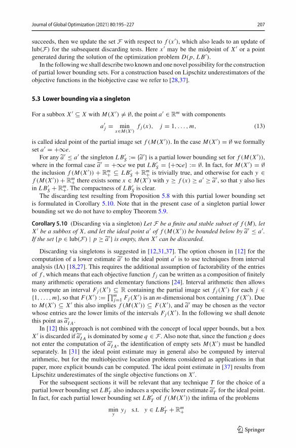
succeeds, then we update the set F with respect to f (x ′), which also leads to an update oflub(F) for the subsequent discarding tests. Here x ′ may be the midpoint of X ′ or a pointgenerated during the solution of the optimization problem D(p, LB ′).
In the followingwe shall describe two known and one novel possibility for the constructionof partial lower bounding sets. For a construction based on Lipschitz underestimators of theobjective functions in the biobjective case we refer to [28,37].
5.3 Lower bounding via a singleton
For a subbox X ′ ⊆ X with M(X ′) �= ∅, the point a′ ∈ Rm with components
a′j = min
x∈M(X ′)f j (x), j = 1, . . . ,m, (13)
is called ideal point of the partial image set f (M(X ′)). In the case M(X ′) = ∅ we formallyset a′ = +∞e.
For any a′ ≤ a′ the singleton LB ′S := {a′} is a partial lower bounding set for f (M(X ′)),
where in the formal case a′ = +∞e we put LB ′S = {+∞e} := ∅. In fact, for M(X ′) = ∅
the inclusion f (M(X ′)) + Rm+ ⊆ LB ′
S + Rm+ is trivially true, and otherwise for each y ∈
f (M(X ′)) + Rm+ there exists some x ∈ M(X ′) with y ≥ f (x) ≥ a′ ≥ a′, so that y also lies
in LB ′S + R
m+. The compactness of LB ′S is clear.
The discarding test resulting from Proposition 5.8 with this partial lower bounding setis formulated in Corollary 5.10. Note that in the present case of a singleton partial lowerbounding set we do not have to employ Theorem 5.9.
Corollary 5.10 (Discarding via a singleton) Let F be a finite and stable subset of f (M), letX ′ be a subbox of X, and let the ideal point a′ of f (M(X ′)) be bounded below by a′ ≤ a′.If the set {p ∈ lub(F) | p ≥ a′} is empty, then X ′ can be discarded.
Discarding via singletons is suggested in [12,31,37]. The option chosen in [12] for thecomputation of a lower estimate a′ to the ideal point a′ is to use techniques from intervalanalysis (IA) [18,27]. This requires the additional assumption of factorability of the entriesof f , which means that each objective function f j can be written as a composition of finitelymany arithmetic operations and elementary functions [24]. Interval arithmetic then allowsto compute an interval Fj (X ′) ⊆ R containing the partial image set f j (X ′) for each j ∈{1, . . . ,m}, so that F(X ′) := ∏m
j=1 Fj (X ′) is an m-dimensional box containing f (X ′). Dueto M(X ′) ⊆ X ′ this also implies f (M(X ′)) ⊆ F(X ′), and a′ may be chosen as the vectorwhose entries are the lower limits of the intervals Fj (X ′). In the following we shall denotethis point as a′
I A.In [12] this approach is not combined with the concept of local upper bounds, but a box
X ′ is discarded if a′I A is dominated by some q ∈ F . Also note that, since the function g does
not enter the computation of a′I A, the identification of empty sets M(X ′) must be handled
separately. In [31] the ideal point estimate may in general also be computed by intervalarithmetic, but for the multiobjective location problems considered as applications in thatpaper, more explicit bounds can be computed. The ideal point estimate in [37] results fromLipschitz underestimates of the single objective functions on X ′.
For the subsequent sections it will be relevant that any technique T for the choice of apartial lower bounding set LB ′
T also induces a specific lower estimate a′T for the ideal point.
In fact, for each partial lower bounding set LB ′T of f (M(X ′)) the infima of the problems
miny
y j s.t. y ∈ LB ′T + R
m+
123
208 Journal of Global Optimization (2021) 80:195–227
with j ∈ {1, . . . ,m} form a vector a′T ≤ a′, that is, a specific lower estimate for the ideal
point of f (M(X ′)). Therefore we obtain the induced singleton partial lower bounding setLB ′
T ,S := {a′T }.
Clearly, in view of Corollary 5.10 a subbox X ′ can be discarded if {p ∈ lub(F) | p ≥ a′T }
is empty. However, due to the relation LB ′T + R
m+ ⊆ a′T + R
m+ we may also modify thegeneral discarding test from Theorem 5.9 as follows.
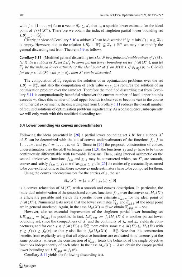
Corollary 5.11 (Modified general discarding test) LetF be a finite and stable subset of f (M),let X ′ be a subbox of X, let LB ′
T be some partial lower bounding set for f (M(X ′)), and leta′T be the induced lower estimate of the ideal point of f on M(X ′). If ϕLB′
T(p) > 0 holds
for all p ∈ lub(F) with p ≥ a′T , then X ′ can be discarded.
The computation of a′T requires the solution of m optimization problems over the set
LB ′T + R
m+, and also the computation of each value ϕLB′T(p) requires the solution of an
optimization problem over the same set. Therefore the modified discarding test from Corol-lary 5.11 is computationally beneficial whenever the current number of local upper boundsexceedsm. Since this number of local upper bounds is observed to become vast in the courseof numerical experiments, the discarding test fromCorollary 5.11 reduces the overall numberof required solutions of optimization problems significantly. As a consequence, subsequentlywe will only work with this modified discarding test.
5.4 Lower bounding via convex underestimators
Following the ideas presented in [26] a partial lower bounding set LB ′ for a subbox X ′of X can be determined with the aid of convex underestimators of the functions f j , j =1, . . . ,m, and gi , i = 1, . . . , k, on X ′. Since in [26] the proposed construction of convexunderestimators uses the αBB technique from [1,3], the functions f j and gi have to be twicecontinuously differentiable with factorable Hessians. Then, using interval arithmetic on thesecond derivatives, functions f j,α and gi,α may be constructed which, on X ′, are smooth,convex and satisfy f j,α ≤ f j aswell as gi,α ≤ gi . In [26] the entries of g are actually assumedto be convex functions, so that there no convex underestimators have to be computed for them.
Using the convex underestimators for the entries of g, the set
Mα(X ′) := {x ∈ X ′ | gα(x) ≤ 0}is a convex relaxation of M(X ′) with a smooth and convex description. In particular, theindividual minimization of the smooth and convex functions f j,α over the convex setMα(X ′)is efficiently possible and yields the specific lower estimate a′
αBB for the ideal point off (M(X ′)). Numerical tests reveal that the lower estimates a′
I A and a′αBB of the ideal point
are in general unrelated. Again, in the case Mα(X ′) = ∅ we obtain a′αBB = +∞e.
However, also an essential improvement of the singleton partial lower bounding setLB ′
αBB,S = {a′αBB} is possible. In fact, LB ′
αBB := fα(Mα(X ′)) is another partial lowerbounding set, since the compactness of X ′ and the continuity of fα and gα yields its com-pactness, and for each y ∈ f (M(X ′)) + R
m+ there exists some x ∈ M(X ′) ⊆ Mα(X ′) withy ≥ f (x) ≥ fα(x), so that y also lies in fα(Mα(X ′)) + R
m+. Note that this constructionbenefits from explicitly using that all objective functions are evaluated simultaneously at thesame points x , whereas the construction of a′
αBB treats the behavior of the single objectivefunctions independently of each other. In the case Mα(X ′) = ∅ we obtain the empty partiallower bounding set LB ′
αBB = fα(∅).Corollary 5.11 yields the following discarding test.
123
Journal of Global Optimization (2021) 80:195–227 209
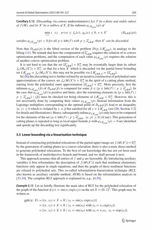
Corollary 5.12 (Discarding via convex underestimators) Let F be a finite and stable subsetof f (M), and let X ′ be a subbox of X. If the infimum ϕLB′
αBB(p) of
mint,x
t s.t. p+te ≥ fα(x), gα(x) ≤ 0, x ∈ X ′ (DαBB(p))
satisfies ϕLB′αBB
(p) > 0 for all p ∈ lub(F) with p ≥ a′αBB, then X ′ can be discarded.
Note that DαBB(p) is the lifted version of the problem D(p, LB ′αBB), in analogy to the
lifting (11). We remark that here the computation of a′αBB requires the solution of m convex
optimization problems, and the computation of each value ϕLB′αBB
(p) requires the solutionof another convex optimization problem.
It is not hard to see that the set {a′αBB} + R
m+ may be essentially larger than its subsetfα(Mα(X ′)) + R
m+, so that for a box X ′ which is discarded via the partial lower boundingset LB ′
αBB = fα(Mα(X ′)), this may not be possible via LB ′αBB,S = {a′
αBB}.In [26] this discarding test is further refined by an iterative construction of polyhedral outer
approximations of the convex set fα(M(X ′)) + Rm+ in the spirit of a cutting plane method,
starting from the polyhedral outer approximation {a′αBB} + R
m+. More precisely, first theinfimum ϕLB′
αBB( p) of DαBB( p) is computed for some p ∈ {p ∈ lub(F) | p ≥ a′
αBB}. Inthe case that ϕLB′
αBB( p) is positive and finite, also the remaining elements in {p ∈ lub(F) |
p ≥ a′αBB} \ { p} must be checked for being elements of LB ′
αBB + Rm+. However, this is
not necessarily done by computing their values ϕLB′αBB
(p). Instead information from theLagrange multipliers corresponding to the optimal point of DαBB( p) lead to an inequality〈a, y〉 ≤ b which is violated by y = p but satisfied for all y ∈ LB ′
αBB (see [26, Section 3.2]for details and illustrations).Hence, subsequently infimaϕLB′
αBB(p)only have to be computed
for the elements of the set {p ∈ lub(F) | p ≥ a′αBB , 〈a, p〉 ≤ b} (if any). This generation of
cutting planes is repeated as long as local upper bounds p with ϕLB′αBB
(p) > 0 are identifiedand speeds up the discarding test significantly.
5.5 Lower bounding via a linearization technique
Instead of constructing polyhedral relaxations of the partial upper image set f (M(X ′))+Rm+
by the generation of cutting planes to a convex relaxation, there is also a more direct methodto generate polyhedral relaxations. To the best of our knowledge this has not yet been usedin the framework of multiobjective branch-and-bound, and we shall present it next.
This approach assumes that all entries of f and g are factorable. By introducing auxiliaryvariables it first reformulates the description of f (M(X ′)) such that nonlinear elementaryfunctions only appear in single equations, and then the graphs of these nonlinear functionsare relaxed to polyhedral sets. This so-called reformulation-linearization technique (RLT,also known as auxiliary variable method; AVM) is based on the reformulation analysis in[33,34]. The complete RLT approach is explained in, e.g., [4,35].
Example 5.13 Let us briefly illustrate the main idea of RLT for the polyhedral relaxation ofthe graph of the function ψ(x) = sin(x1 exp(x2)) on the set X = [0, 1]2. This graph may bewritten as
gph(ψ, X) = {(x, x3) ∈ X × R | x3 = sin(x1 exp(x2))}= {(x, x3) ∈ X × R | x3 = sin(x4) with x4 = x1 exp(x2)}= {(x, x3) ∈ X × R | x3 = sin(x4) with x4 = x1x5, x5 = exp(x2)}.
123
210 Journal of Global Optimization (2021) 80:195–227
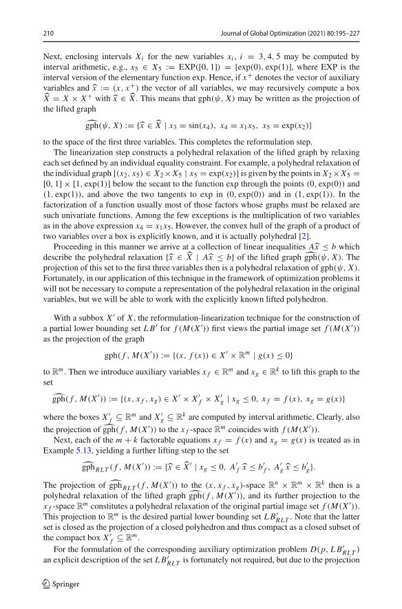
Next, enclosing intervals Xi for the new variables xi , i = 3, 4, 5 may be computed byinterval arithmetic, e.g., x5 ∈ X5 := EXP([0, 1]) = [exp(0), exp(1)], where EXP is theinterval version of the elementary function exp. Hence, if x+ denotes the vector of auxiliaryvariables and x := (x, x+) the vector of all variables, we may recursively compute a boxX = X × X+ with x ∈ X . This means that gph(ψ, X) may be written as the projection ofthe lifted graph
gph(ψ, X) := {x ∈ X | x3 = sin(x4), x4 = x1x5, x5 = exp(x2)}to the space of the first three variables. This completes the reformulation step.
The linearization step constructs a polyhedral relaxation of the lifted graph by relaxingeach set defined by an individual equality constraint. For example, a polyhedral relaxation ofthe individual graph {(x2, x5) ∈ X2×X5 | x5 = exp(x2)} is given by the points in X2×X5 =[0, 1] × [1, exp(1)] below the secant to the function exp through the points (0, exp(0)) and(1, exp(1)), and above the two tangents to exp in (0, exp(0)) and in (1, exp(1)). In thefactorization of a function usually most of those factors whose graphs must be relaxed aresuch univariate functions. Among the few exceptions is the multiplication of two variablesas in the above expression x4 = x1x5. However, the convex hull of the graph of a product oftwo variables over a box is explicitly known, and it is actually polyhedral [2].
Proceeding in this manner we arrive at a collection of linear inequalities Ax ≤ b whichdescribe the polyhedral relaxation {x ∈ X | Ax ≤ b} of the lifted graph gph(ψ, X). Theprojection of this set to the first three variables then is a polyhedral relaxation of gph(ψ, X).Fortunately, in our application of this technique in the framework of optimization problems itwill not be necessary to compute a representation of the polyhedral relaxation in the originalvariables, but we will be able to work with the explicitly known lifted polyhedron.
With a subbox X ′ of X , the reformulation-linearization technique for the construction ofa partial lower bounding set LB ′ for f (M(X ′)) first views the partial image set f (M(X ′))as the projection of the graph
gph( f , M(X ′)) := {(x, f (x)) ∈ X ′ × Rm | g(x) ≤ 0}
to Rm . Then we introduce auxiliary variables x f ∈ R
m and xg ∈ Rk to lift this graph to the
set
gph( f , M(X ′)) := {(x, x f , xg) ∈ X ′ × X ′f × X ′
g | xg ≤ 0, x f = f (x), xg = g(x)}where the boxes X ′
f ⊆ Rm and X ′
g ⊆ Rk are computed by interval arithmetic. Clearly, also
the projection of gph( f , M(X ′)) to the x f -space Rm coincides with f (M(X ′)).
Next, each of the m + k factorable equations x f = f (x) and xg = g(x) is treated as inExample 5.13, yielding a further lifting step to the set
gphRLT ( f , M(X ′)) := {x ∈ X ′ | xg ≤ 0, A′f x ≤ b′
f , A′g x ≤ b′
g}.The projection of gphRLT ( f , M(X ′)) to the (x, x f , xg)-space R
n × Rm × R
k then is apolyhedral relaxation of the lifted graph gph( f , M(X ′)), and its further projection to thex f -space R
m constitutes a polyhedral relaxation of the original partial image set f (M(X ′)).This projection to R
m is the desired partial lower bounding set LB ′RLT . Note that the latter
set is closed as the projection of a closed polyhedron and thus compact as a closed subset ofthe compact box X ′
f ⊆ Rm .
For the formulation of the corresponding auxiliary optimization problem D(p, LB ′RLT )
an explicit description of the set LB ′RLT is fortunately not required, but due to the projection
123
Journal of Global Optimization (2021) 80:195–227 211
property we may as well solve the lifted problem
mint ,x
t s.t. p+te ≥ x f , xg ≤ 0, A′f x ≤ b′
f , A′g x ≤ b′
g, x ∈ X ′, (DRLT (p))
that is, a box constrained linear program. Corollary 5.11 thus yields the following discardingtest, where the entries of the corresponding lower estimate a′
RLT of the ideal point of f onM(X ′) are the optimal values of the m linear optimization problems
minx
(x f ) j s.t. xg ≤ 0, A′f x ≤ b′
f , A′g x ≤ b′
g, x ∈ X ′
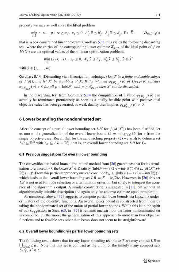
with j ∈ {1, . . . ,m}.Corollary 5.14 (Discarding via a linearization technique) Let F be a finite and stable subsetof f (M), and let X ′ be a subbox of X. If the infimum ϕLB′
RLT(p) of DRLT (p) satisfies
ϕLB′RLT
(p) > 0 for all p ∈ lub(F) with p ≥ a′RLT , then X ′ can be discarded.
In the discarding test from Corollary 5.14 the computation of a value ϕLB′RLT
(p) canactually be terminated prematurely as soon as a dually feasible point with positive dualobjective value has been generated, as weak duality then implies ϕLB′
RLT(p) > 0.
6 Lower bounding the nondominated set
After the concept of a partial lower bounding set LB ′ for f (M(X ′)) has been clarified, letus turn to the generalization of the overall lower bound �b = minX ′∈L �b′ for v from thesingle objective case. Recall that for the sandwiching property (2) we wish to define a setLB ⊆ R
m with YN ⊆ LB + Rm+, that is, an overall lower bounding set LB for YN .
6.1 Previous suggestions for overall lower bounding
The convexification based branch-and-bound method from [26] guarantees that for its termi-nation tolerance ε > 0 the boxes X ′ ∈ L satisfy (lub(F)−(ε/2)e−int(Rm+))∩( fα(M(X ′))+Rm+) = ∅. From this particular property one can concludeYN ⊆ (lub(F)−(ε/2)e−int(Rm+))c
which leads to the overall lower bounding set LB = F − (ε/2)e. However, in [26] this setLB is not used for node selection or a termination criterion, but solely to interpret the accu-racy of the algorithm’s output. A similar construction is suggested in [11], but without analgorithmically suitable description and again only for an error estimate upon termination.
As mentioned above, [37] suggests to compute partial lower bounds via Lipschitz under-estimators of the objective functions. An overall lower bound is constructed from them bytaking the nondominated set of the union of partial lower bounds. While this is in the spiritof our suggestion in Sect. 6.3, in [37] it remains unclear how the latter nondominated setis computed. Furthermore, the generalization of this approach to more than two objectivefunctions and to feasible sets other than boxes does not seem to be straightforward.
6.2 Overall lower bounding via partial lower bounding sets
The following result shows that for any lower bounding technique T we may choose LB =⋃X ′∈L LB ′
T . Note that this set is compact as the union of the finitely many compact setsLB ′
T , X′ ∈ L.
123
212 Journal of Global Optimization (2021) 80:195–227
Lemma 6.1 For any lower bounding technique T and partial lower bounding sets LB′T for
f (M(X ′)) define LBT := ⋃X ′∈L LB ′
T . Then the inclusion
YN ⊆ LBT + Rm+
holds.
Proof Corresponding to any yN ∈ YN there exists some efficient point xE ∈ M(X) withyN = f (xE ). Assume that the subbox X ′
E with xE ∈ M(X ′E ) does not lie in L. Then it has
been discarded, and since all discussed discarding tests are based on the general condition(12) from Proposition 5.8 with the set of local upper bounds lub(F) of some provisionalnondominated set F , the box X ′
E also satisfies (8) with this set lub(F). Proposition 5.3 thusyields YN ∩ ( f (M(X ′
E )) + Rm+) = ∅ which contradicts yN ∈ f (M(X ′
E )). Consequentlythere is some X ′
E ∈ L with yN ∈ f (M(X ′E )) which implies
yN ∈ f (M(X ′E )) + R
m+ ⊆ LB ′T ,E + R
m+ ⊆(
⋃
X ′∈LLB ′
T
)
+ Rm+
and shows the assertion. �In view of YN �= ∅ Lemma 6.1 particularly guarantees LBT �= ∅. More importantly,
together with (7) we have shown that the desired enclosing property (2) for the nondominatedset YN may in fact be formulated as
YN ⊆ (LBT + R
m+) ∩ (
lub(F) − Rm+), (14)
that is, the enclosure E(LBT , lub(F)) satisfies (2).In the single objective case it is clear that not only the function value v = f (xmin) of
any minimal point xmin lies in the enclosing interval [�b, ub], but also the function valuef (xub) = ub of the currently best known feasible point. In the multiobjective setting thiscorresponds to the set E(LBT , lub(F)) not only enclosing the nondominated set YN , but alsothe provisional nondominated set F = f (Xub). The following result verifies this.
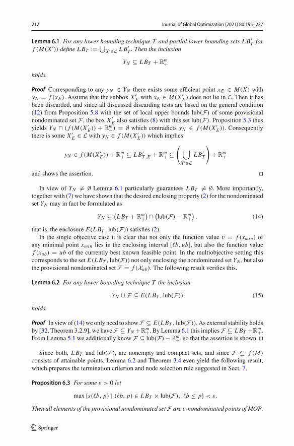
Lemma 6.2 For any lower bounding technique T the inclusion
YN ∪ F ⊆ E(LBT , lub(F)) (15)
holds.
Proof In viewof (14)we only need to showF ⊆ E(LBT , lub(F)). As external stability holdsby [32, Theorem 3.2.9], we haveF ⊆ YN +R
m+. By Lemma 6.1 this impliesF ⊆ LBT +Rm+.
From Lemma 5.1 we additionally know F ⊆ lub(F) − Rm+, so that the assertion is shown. �
Since both, LBT and lub(F), are nonempty and compact sets, and since F ⊆ f (M)
consists of attainable points, Lemma 6.2 and Theorem 3.4 even yield the following result,which prepares the termination criterion and node selection rule suggested in Sect. 7.
Proposition 6.3 For some ε > 0 let
max {s(�b, p) | (�b, p) ∈ LBT × lub(F), �b ≤ p} < ε.
Then all elements of the provisional nondominated setF are ε-nondominated points of MOP.
123
Journal of Global Optimization (2021) 80:195–227 213
6.3 Overall lower bounding by nondominated ideal point estimates
For efficient handling of the set LBT + Rm+ = ⋃
X ′∈L(LB ′
T + Rm+)in the definition of
the enclosure E(LBT , lub(F)) as well as in the resulting termination criterion and nodeselection rule, one should take into account that many boxes X ′ ∈ Lmay be redundant in itsdescription. In the single objective case this corresponds to the fact that most X ′ ∈ L satisfy�b′ > �b = minX ′∈L �b′, so that we are only interested in a box X ′ with �b′ = �b. Usuallythe latter box is unique. In the multiobjective setting one cannot expect the existence of asingle box X ′ with LB ′
T + Rm+ = LBT + R
m+, but several boxes X ′ may be nonredundant,namely the ones for which the sets LB ′
T are ‘nondominated’ in some sense.A situation for which nondominance among the sets LB ′
T , X′ ∈ L, is easily defined is the
case of singleton sets LB ′T . Hence, for each X ′ ∈ L let us again consider the lower estimate
a′T for the ideal point of f (M(X ′)) induced by LB ′
T . Recall that LB′T ,S = {a′
T } is a singletonpartial lower bounding set for f (M(X ′)), so that by Lemma 6.1 the finite set
LBT ,S = {a′T | X ′ ∈ L}
is an overall lower bounding set, that is, YN ⊆ LBT ,S + Rm+ holds.
Let us now consider only boxes X ′ ∈ L which correspond to the nondominated points ofLBT ,S , that is, to the (unique) stable subset LBT ,S,N of LBT ,S so that no element of LBT ,S,N
is dominated by some point in LBT ,S .
Lemma 6.4 With the nondominated set LBT ,S,N of LBT ,S the inclusions
LBT + Rm+ ⊆ LBT ,S + R
m+ ⊆ LBT ,S,N + Rm+
hold.
Proof The first inclusion is valid because of
LBT + Rm+ =
(⋃
X ′∈LLB ′
T
)
+ Rm+ =
⋃
X ′∈L(LB ′
T + Rm+) ⊆
⋃
X ′∈L({a′
T } + Rm+)
=(
⋃
X ′∈L{a′
T })
+ Rm+ = LBT ,S + R
m+.
Furthermore, for each y ∈ LBT ,S + Rm+ there is some X ′ ∈ L with a′
T ≤ y. As |L| < ∞,either a′
T ∈ LBT ,S,N holds or there exists some a ∈ LBT ,S,N with a ≤ a′T ≤ y. This shows
the second inclusion. �The first inclusion in the assertion of Lemma 6.4 means that, as expected, LBT ,S is a coarseroverall lower bound for YN ∪ F than LBT . The second inclusion implies that the ‘relevant’boxes for the definition of LBT ,S + R
m+ are the ones from the sublist
LN := {X ′ ∈ L | a′T ∈ LBT ,S,N }.
The combination of Lemma 6.2 with Lemma 6.4 and (3) immediately yields the nextresult.
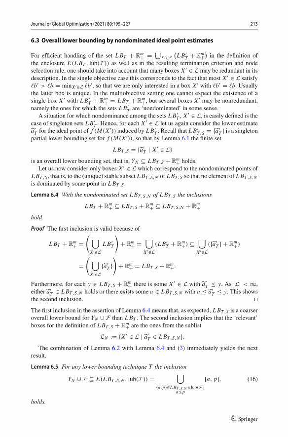
Lemma 6.5 For any lower bounding technique T the inclusion
YN ∪ F ⊆ E(LBT ,S,N , lub(F)) =⋃
(a,p)∈LBT ,S,N×lub(F)a≤p
[a, p]. (16)
holds.
123
214 Journal of Global Optimization (2021) 80:195–227
7 Termination criterion, node selection rule, and conceptual algorithm
In view of Lemma 6.5 and Theorem 3.4 we can now state the basis for the terminationcriterion of the multiobjective branch-and-bound method.
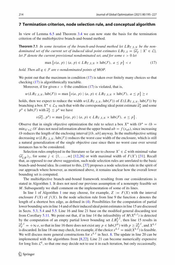
Theorem 7.1 In some iteration of the branch-and-bound method let LBT ,S,N be the non-dominated set of the current set of induced ideal point estimates LBT ,S = {a′
T | X ′ ∈ L},let F denote the current provisional nondominated set, and for some ε > 0 let
max{s(a, p) | (a, p) ∈ LBT ,S,N × lub(F), a ≤ p
}< ε (17)
hold. Then all q ∈ F are ε-nondominated points of MOP.
We point out that the maximum in condition (17) is taken over finitely many choices so thatchecking (17) is algorithmically tractable.
Moreover, if for given ε > 0 the condition (17) is violated, that is,
w(LBT ,S,N , lub(F)) = max{s(a, p) | (a, p) ∈ LBT ,S,N × lub(F), a ≤ p
} ≥ ε
holds, then we expect to reduce the width w(LBT ,S,N , lub(F)) of E(LBT ,S,N , lub(F)) bybranching a box X� ∈ LN such that with the corresponding ideal point estimate a�
T and somep� ∈ lub(F) with a�
T ≤ p� we have
s (a�T , p�) = max
{s(a, p) | (a, p) ∈ LBT ,S,N × lub(F), a ≤ p
}.
Observe that in single objective optimization the rule to select a box X� with �b� = �b =minX ′∈L �b′ does not need information about the upper bound ub = f (xub), since increasing�b reduces the length of the enclosing interval [�b, ub] anyway. In the multiobjective settingdecreasing w(LBT ,S,N , lub(F)) reduces the worst case width of the enclosure, which is stilla natural generalization of the single objective case since there no worst case over severalinstances has to be considered.
Selection rules employed in the literature so far are to choose X ′ ∈ L with minimal value(a′
LB′) j , for some j ∈ {1, . . . ,m} [12,26] or with maximal width of F(X ′) [31]. Recallthat, as opposed to our above suggestion, such node selection rules are unrelated to the basicbranch-and-bound idea. In contrast to this, [37] proposes a node selection rule in the spirit ofour approach where however, as mentioned above, it remains unclear how the overall lowerbounding set is computed.
The multiobjective branch-and-bound framework resulting from our considerations isstated in Algorithm 1. It does not need our previous assumption of a nonempty feasible setM . Subsequently we shall comment on the implementation of some of its lines.
In line 1 of Algorithm 1 one may choose, for example, Z := F(X) with the intervalenclosure F(X) of f (X). In the node selection rule from line 9 the function s denotes thelength of a shortest box edge, as defined in (4). Possibilities for the computation of partiallower bounding sets in line 14 andof their induced ideal point estimates in line 15 are discussedin Sects. 5.3, 5.4 and 5.5. Line 16 and line 21 base on the modified general discarding testfrom Corollary 5.11. We point out that, if in line 14 the infeasibility of M(Xk,�) is detectedby the computation of an empty partial lower bounding set LBk,�
T , then line 15 results in
ak,�T = +∞ e, so that in line 16 there does not exist any p ∈ lub(Fk)with p ≥ ak,�T , and Xk,�
is discarded. In line 18 onemay check, for example, if the choice xk,� = mid(Xk,�) is feasible.We will discuss more general constructions for xk,� in Sect. 8. The update in line 20 can beimplemented with the algorithms from [8,22]. Line 21 can become numerically expensivefor long lists Lk , so that one may decide not to use it in each iteration, but only occasionally.
123
Journal of Global Optimization (2021) 80:195–227 215
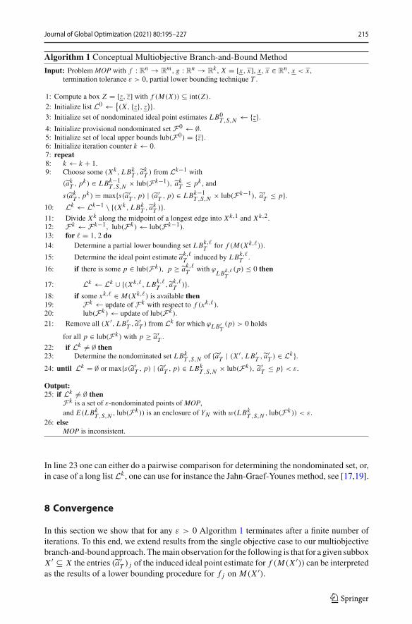
Algorithm 1 Conceptual Multiobjective Branch-and-Bound Method
Input: Problem MOP with f : Rn → R
m , g : Rn → R
k , X = [x, x], x, x ∈ Rn , x < x ,
termination tolerance ε > 0, partial lower bounding technique T .
1: Compute a box Z = [z, z] with f (M(X)) ⊆ int(Z).2: Initialize list L0 ← {
(X , {z}, z)}.3: Initialize set of nondominated ideal point estimates LB0
T ,S,N ← {z}.4: Initialize provisional nondominated set F0 ← ∅.5: Initialize set of local upper bounds lub(F0) = {z}.6: Initialize iteration counter k ← 0.7: repeat8: k ← k + 1.9: Choose some (Xk , LBk
T , akT ) from Lk−1 with
(akT , pk ) ∈ LBk−1T ,S,N × lub(Fk−1), akT ≤ pk , and
s (akT , pk ) = max{s (a′T , p) | (a′
T , p) ∈ LBk−1T ,S,N × lub(Fk−1), a′
T ≤ p}.10: Lk ← Lk−1 \ {(Xk , LBk
T , akT )}.11: Divide Xk along the midpoint of a longest edge into Xk,1 and Xk,2.12: Fk ← Fk−1, lub(Fk ) ← lub(Fk−1).13: for � = 1, 2 do14: Determine a partial lower bounding set LBk,�
T for f (M(Xk,�)).
15: Determine the ideal point estimate ak,�T induced by LBk,�T .
16: if there is some p ∈ lub(Fk ), p ≥ ak,�T with ϕLBk,�T
(p) ≤ 0 then
17: Lk ← Lk ∪ {(Xk,�, LBk,�T , ak,�T )}.
18: if some xk,� ∈ M(Xk,�) is available then19: Fk ← update of Fk with respect to f (xk,�).20: lub(Fk ) ← update of lub(Fk ).21: Remove all (X ′, LB′
T , a′T ) from Lk for which ϕLB′
T(p) > 0 holds
for all p ∈ lub(Fk ) with p ≥ a′T .
22: if Lk �= ∅ then23: Determine the nondominated set LBk
T ,S,N of {a′T | (X ′, LB′
T , a′T ) ∈ Lk }.
24: until Lk = ∅ or max{s (a′T , p) | (a′
T , p) ∈ LBkT ,S,N × lub(Fk ), a′
T ≤ p} < ε.
Output:25: if Lk �= ∅ then
Fk is a set of ε-nondominated points of MOP,and E(LBk
T ,S,N , lub(Fk )) is an enclosure of YN with w(LBkT ,S,N , lub(Fk )) < ε.
26: elseMOP is inconsistent.
In line 23 one can either do a pairwise comparison for determining the nondominated set, or,in case of a long listLk , one can use for instance the Jahn-Graef-Younes method, see [17,19].
8 Convergence
In this section we show that for any ε > 0 Algorithm 1 terminates after a finite number ofiterations. To this end, we extend results from the single objective case to our multiobjectivebranch-and-bound approach. Themain observation for the following is that for a given subboxX ′ ⊆ X the entries (a′
T ) j of the induced ideal point estimate for f (M(X ′)) can be interpretedas the results of a lower bounding procedure for f j on M(X ′).
123
216 Journal of Global Optimization (2021) 80:195–227
In preparation of the convergence proof we briefly review the definition and some impor-tant properties of such lower bounding procedures in the single objective branch-and-boundframework. As common in global optimization, a sequence of boxes (Xk) is called exhaustiveif we have Xk+1 ⊆ Xk for all k ∈ N, and limk diag(Xk) = 0 where diag(X ′) denotes thediagonal length of a box X ′ ⊆ X . The following definitions are taken from [20].
Definition 8.1 Let f : Rn → R, g : R
m → Rk and M(X) = {x ∈ X | g(x) ≤ 0}.
(a) A function � from the set of all subboxes X ′ of X to R ∪ {+∞} is called M-dependentlower bounding procedure if �(X ′) ≤ inf x∈M(X ′) f (x) holds for all subboxes X ′ ⊆ Xand any choice of the functions f and g.
(b) An M-dependent lower bounding procedure is called convergent if every exhaustivesequence of boxes (Xk) and all choices of f and g satisfy
limk
�(Xk) = limk
infx∈M(Xk )
f (x).
We remark that for any exhaustive sequence of boxes (Xk) the set⋂
k∈N Xk is a singleton,say {x}. In the case x /∈ M(X) we have M(Xk) = ∅ for all sufficiently large k, so that withthe usual convention infx∈∅ f (x) = +∞ the convergence of a lower bounding procedurethen requires limk �(Xk) = +∞. Moreover, if in the case x ∈ M(X) we have xk ∈ Xk
for all k, then in view of limk diag(Xk) = 0 the sequence (xk) also converges to x , and theconvergence of � and continuity yield
limk
�(Xk) = limk
infx∈M(Xk )
f (x) = f (x) = limk
f (xk). (18)
Basically all lower bounding procedures that are commonly used in global optimizationare convergent in the sense of Definition 8.1, in particular the ones considered throughout thisarticle, that is, interval arithmetic [18,27], convex relaxations via the αBB method [1,3] aswell as lower bounds based on linearization techniques as described in [4,33–35]. Note thatin the above case x /∈ M(X) these lower bounding procedures even satisfy �(Xk) = +∞ foralmost all k, thus implying the convergence property limk �(Xk) = +∞. While this strongerproperty is employed for discarding inconsistent subproblems in line 16 of Algorithm 1, wewill not use it in our convergence analysis.
As mentioned above, in Algorithm 1 the entries (a′T ) j of the induced ideal point estimate
for f (M(X ′)) are the results �T , j (X ′) of a lower bounding procedure �T , j for f j on M(X ′).For the following let �T (X ′) denote the vector with entries �T , j (X ′), so that we may writea′T = �T (X ′).We start by showing that problems with empty feasible sets are handled by our branch-
and-bound method as expected.
Lemma 8.2 Let the feasible set of problemMOP be empty and assume that in Algorithm 1 theentries of the induced ideal point estimates are computed by some convergent M-dependentlower bounding procedure. Then for any ε > 0 Algorithm 1 terminates after a finite numberof iterations.
Proof We assume the contrary and derive a contradiction. First of all, note that due to theabsenceof feasible points the local upper bounds are never updated, so thatwehave lub(Fk) ={z} in each iteration k.
Under our assumption that the algorithm does not terminate it is well-known from thetheory of spatial branch-and-bound methods that an exhaustive sequence of boxes (Xkν ) isgenerated. Since none of these boxes contains a point from M(X), the convergence of the
123
Journal of Global Optimization (2021) 80:195–227 217
lower bounding procedure yields �T (Xkν ) = akν
T > z for some sufficiently large ν. Thus inline 16 of Algorithm 1 the box Xkν is discarded. For that reason, the sequence of boxes (Xkν )
actually terminates after finitely many iterates and cannot be exhaustive. �Analogously to the single objective case, we must assume that in line 18 of Algorithm 1
feasible points are eventually available to improve the local upper bounds. This is formallystated in the following assumption, which we shall discuss in some detail after the proof ofconvergence.
Assumption 8.3 There exist some δ > 0 and some procedure so that for all boxes X ′ ⊆ Xcreated by Algorithm 1 with diag(X ′) < δ and M(X ′) �= ∅ a feasible point x ′ ∈ M(X ′) canbe computed.
Lemma 8.4 Let the feasible set of problemMOP be nonempty, assume that in Algorithm 1 theentries of the induced ideal point estimates are computed by some convergent M-dependentlower bounding procedure, and let Assumption 8.3 hold. Then for any ε > 0 Algorithm 1terminates after a finite number of iterations.
Proof Assume that the algorithmdoes not terminate. Then it generates an exhaustive sequenceof boxes (Xkν ) all of which contain a feasible point. Note that otherwise the sequence ofboxes would terminate after finitely many iterations, for a similar reason as in the proofof Lemma 8.2 (see, e.g., [20] for a more detailed explanation). As the sequence (Xkν ) isexhaustive and due to Assumption 8.3, for all sufficiently large ν a point xkν ∈ M(Xkν )
is available in line 18 of Algorithm 1. Since the image point f (xkν ) is used to update theprovisional nondominated set in line 19, it either becomes an element of Fkν or it is ignoredsince it is dominated by some point from Fkν . In any case, there is some qkν ∈ Fkν with
qkν ≤ f (xkν ). (19)
Due to (18), for some sufficiently large ν ∈ N we additionally have
f (xkν ) − �T (Xkν ) ≤ ε
2e, (20)
where e again stands for the all ones vector. Finally, as the termination criterion was violatedin iteration kν − 1, the ideal point estimate akν
T ∈ LBkν−1T ,S,N and the local upper bound
pkν ∈ lub(Fkν−1) with akν
T ≤ pkν , in which the maximum is attained, satisfy
pkν − �T (Xkν ) = pkν − akν
T ≥ εe,
and thus�T (Xkν ) + ε
2e ≤ pkν − ε
2e. (21)
The combination of (19), (20) and (21) yields the chain of inequalities
qkν ≤ f (xkν ) ≤ �T (Xkν ) + ε
2e ≤ pkν − ε
2e < pkν
and, thus, qkν < pkν . This contradicts property (ii) of Definition 4.1 and, hence, the assertionis shown. �From Lemma 8.2 and Lemma 8.4 we immediately obtain the main convergence theorem ofthe present article.
123
218 Journal of Global Optimization (2021) 80:195–227
Theorem 8.5 Assume that in Algorithm 1 the entries of the induced ideal point estimatesare computed by some convergent M-dependent lower bounding procedure, and let Assump-tion 8.3 hold. Then for any ε > 0 Algorithm 1 terminates after a finite number of iterations.
Since, as discussed above, in global optimization usually convergent lower boundingprocedures are used, the seemingly restrictive assumption of Theorem 8.5 is Assumption 8.3.In the remainder of this section we shall briefly comment on this. First note that the difficultyof finding feasible points also arises in single objective branch-and-bound methods: In casethat no sufficiently good feasible point is found, the algorithms do not terminate since thegap between upper and lower bound does not drop below the termination tolerance ε.
Usually the objective function is evaluated at feasible points in order to obtain upperbounds at the globally minimal value. These feasible points can be obtained by means ofdifferent approaches. In a very simple case one may check if the midpoint of a box thatis currently examined is feasible and use this for an update of the current upper bound, ifthe objective value is sufficiently good. In practice, commonly a local procedure is used tosolve the original problem locally where, for instance, the midpoint of the current box isused to initialize the starting point. Under Assumption 8.3 one may eventually expect thebox midpoint to lie sufficiently close to the feasible set to make this local concept work.Although this approach in fact works well on many instances of practical interest, in generalthere is no guarantee that always sufficiently good upper bounds are computed in this way.
One possibility to transfer this approach from the single objective case to multiobjectivebranch-and-bound problems might be to consider a scalarization approach and solve theresulting single objective problem locally. However, although this attempt might work inpractice, we prefer to not follow this line of research here since the drawback of this approachfrom the single objective case still remains and, in general, there is no proof of convergence.
Instead, in single objective optimization it is often proposed to accept so-called εM -feasiblepoints, meaning that a point x ∈ X is accepted if gi (x) ≤ εM , i ∈ {1, . . . , k}, holds for somepredefined value εM > 0. Unfortunately, a reasonable value for εM is hard to determine inadvance, since even for εM close to zero usually one cannot be sure that an εM -feasible pointis actually close to the feasible set.
For that reason, so-called upper bounding procedures have been developed that ensureAssumption 8.3 and, thus, termination of a branch-and-bound method by computing a con-vergent sequence of upper bounds, as for instance proposed in [20] for the purely inequalityconstrained case. For problems that also involve equality constraints we refer to [14]. Thesetechniques can be adapted to multiobjective problems which is, however, beyond the scopeof the present paper.
9 Numerical illustrations
The present section provides a brief proof of concept for Algorithm 1. Note that we neitheraim at studying its numerical behavior for increasing dimensions m and n, nor do we intendto compare the performance of the lower bounding procedures from Sects. 5.3, 5.4 and 5.5among each other or in comparison to other lower bounding procedures like, for example,Lipschitz based underestimators. In fact, a thorough numerical study is beyond the scope ofthe present paper and postponed to future research. In contrast, the aim of the article at handis the introduction of a general framework which allows to consider such comparisons in thefirst place.
123
Journal of Global Optimization (2021) 80:195–227 219
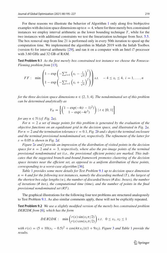
For these reasons we illustrate the behavior of Algorithm 1 only along five biobjectiveexampleswith decision space dimensions up to n = 4,where for threemerely box constrainedinstances we employ interval arithmetic as the lower bounding technique T , while for thetwo instances with additional constraints we test the linearization technique from Sect. 5.5.The box removal step from line 21 is performed only in every 50th iteration to speed up thecomputation time. We implemented the algorithm in Matlab 2019 with the Intlab Toolbox(version 6) for interval arithmetic [29], and ran it on a computer with an Intel i7 processorwith 3.60 GHz and 32 GB of RAM.
Test Problem 9.1 As the first merely box constrained test instance we choose the Fonseca-Fleming problem from [13],
FF : min
⎛
⎜⎜⎝
1 − exp
(
−∑ni=1
(xi − 1√
n
)2)
1 − exp
(
−∑ni=1
(xi + 1√
n
)2)
⎞
⎟⎟⎠ s.t. − 4 ≤ xi ≤ 4, i = 1, . . . , n
for the three decision space dimensions n ∈ {2, 3, 4}. The nondominated set of this problemcan be determined analytically as
YN ={(
1 − exp(−4(t − 1)2)1 − exp(−4t2)
)
| t ∈ [0, 1]}
for any n ∈ N (cf. Fig. 2a).For n = 2 a set of image points for this problem is generated by the evaluation of the
objective functions on an equidistant grid in the decision space, and illustrated in Fig. 2a.For n = 2 and the termination tolerance ε = 0.1, Fig. 2b and c depict the terminal enclosureand the terminal provisional nondominated set, respectively. The refinement of the latter forε = 0.05 is shown in Fig. 2d.
Figure 2e and f provide an impression of the distribution of visited points in the decisionspace for n = 2 and n = 3, respectively, where also the pre-image points of the terminalprovisional nondominated set (i.e., the provisional efficient points) are marked. This indi-cates that the suggested branch-and-bound framework promotes clustering of the decisionspace iterates near the efficient set, as opposed to a uniform distribution of these points,corresponding to a worst-case algorithm [36].
Table 1 provides some more details for Test Problem 9.1 up to decision space dimensionn = 4 and for the following test instances, namely the discarding method (T ), the largest ofthe shortest box edge lengths (w), the number of discarded boxes (# disc. boxes), the numberof iterations (# iter.), the computational time (time), and the number of points in the finalprovisional nondominated set (#F).
The graphical illustrations for the following four test problems are structured analogouslyto Test Problem 9.1. As also similar comments apply, these will not be explicitly repeated.
Test Problem 9.2 We use a slightly modified version of the merely box constrained problemDEB2DK from [6], which has the form
DEB2DK : min
(r(x) sin(x1π/2)r(x) cos(x1π/2)
)
s.t . 0 ≤ x1, x2 ≤ 1
with r(x) = (5 + 10(x1 − 0.5)2 + cos(4πx1))(1 + 9x2). Figure 3 and Table 1 provide theresults.
123
220 Journal of Global Optimization (2021) 80:195–227
(a) (b)
(c)
(e) (f)
(d)
Fig. 2 Test problem FF (Fonseca–Fleming)
Test Problem 9.3 This problem consists of two Shekel functions which are well known fromevaluations of single-objective global optimization algorithms (see, e.g., [28]).
Shekel : min
(− 0.10.1+(x1−0.1)2+2(x2−0.1)2
− 0.10.14+20((x1−0.45)2+(x2−0.55)2)
− 0.10.15+40((x1−0.55)2+(x2−0.45)2)
− 0.10.1+(x1−0.3)2+(x2−0.95)2
)
s.t. 0 ≤ x1, x2 ≤ 1.
123
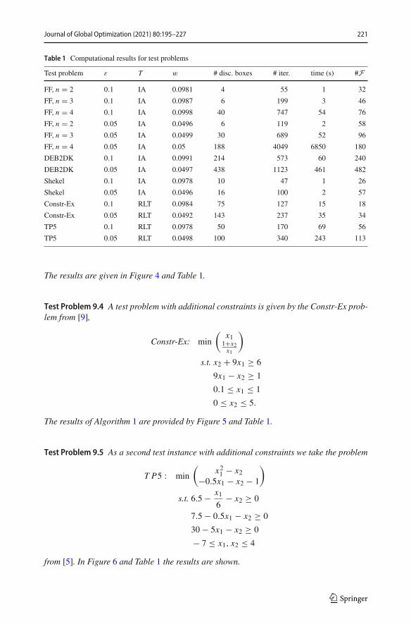
Journal of Global Optimization (2021) 80:195–227 221
Table 1 Computational results for test problems
Test problem ε T w # disc. boxes # iter. time (s) #F
FF, n = 2 0.1 IA 0.0981 4 55 1 32
FF, n = 3 0.1 IA 0.0987 6 199 3 46
FF, n = 4 0.1 IA 0.0998 40 747 54 76
FF, n = 2 0.05 IA 0.0496 6 119 2 58
FF, n = 3 0.05 IA 0.0499 30 689 52 96
FF, n = 4 0.05 IA 0.05 188 4049 6850 180
DEB2DK 0.1 IA 0.0991 214 573 60 240
DEB2DK 0.05 IA 0.0497 438 1123 461 482
Shekel 0.1 IA 0.0978 10 47 1 26
Shekel 0.05 IA 0.0496 16 100 2 57
Constr-Ex 0.1 RLT 0.0984 75 127 15 18
Constr-Ex 0.05 RLT 0.0492 143 237 35 34
TP5 0.1 RLT 0.0978 50 170 69 56
TP5 0.05 RLT 0.0498 100 340 243 113
The results are given in Figure 4 and Table 1.
Test Problem 9.4 A test problem with additional constraints is given by the Constr-Ex prob-lem from [9],
Constr-Ex: min
(x1
1+x2x1
)
s.t. x2 + 9x1 ≥ 6
9x1 − x2 ≥ 1
0.1 ≤ x1 ≤ 1
0 ≤ x2 ≤ 5.
The results of Algorithm 1 are provided by Figure 5 and Table 1.
Test Problem 9.5 As a second test instance with additional constraints we take the problem
T P5 : min
(x21 − x2
−0.5x1 − x2 − 1
)
s.t. 6.5 − x16
− x2 ≥ 0
7.5 − 0.5x1 − x2 ≥ 0
30 − 5x1 − x2 ≥ 0
− 7 ≤ x1, x2 ≤ 4
from [5]. In Figure 6 and Table 1 the results are shown.
123
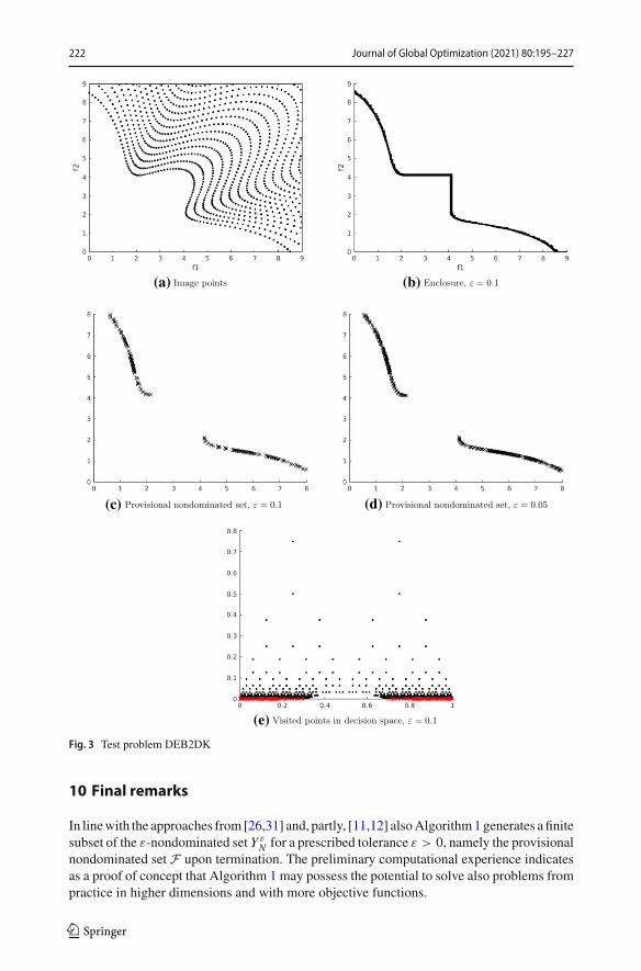
222 Journal of Global Optimization (2021) 80:195–227
(a) (b)
(c) (d)
(e)
Fig. 3 Test problem DEB2DK
10 Final remarks
In linewith the approaches from [26,31] and, partly, [11,12] alsoAlgorithm1generates afinitesubset of the ε-nondominated set Y ε
N for a prescribed tolerance ε > 0, namely the provisionalnondominated set F upon termination. The preliminary computational experience indicatesas a proof of concept that Algorithm 1 may possess the potential to solve also problems frompractice in higher dimensions and with more objective functions.
123
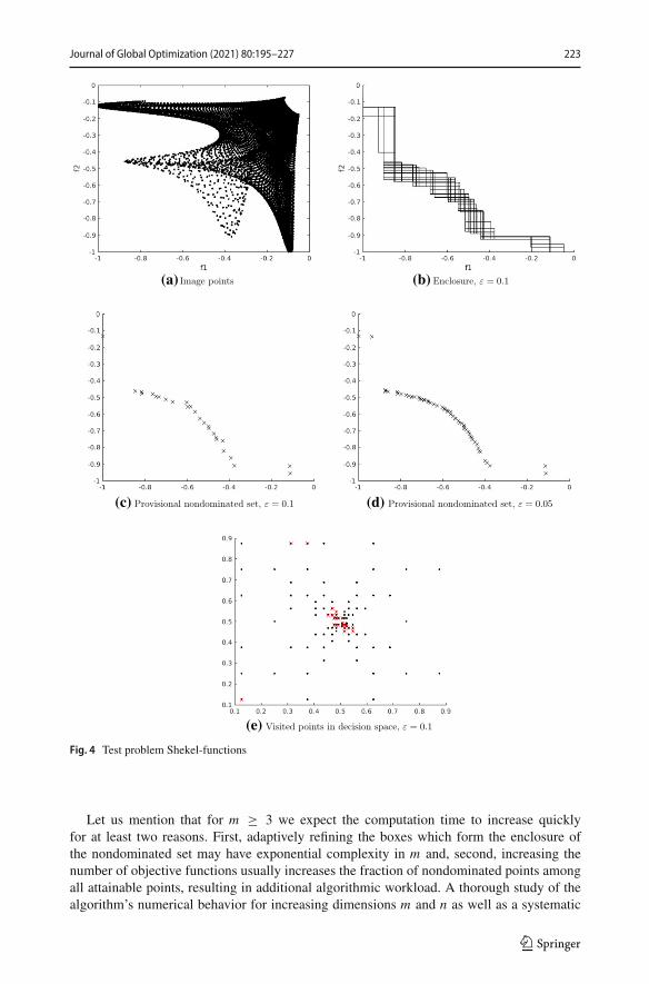
Journal of Global Optimization (2021) 80:195–227 223
(e)
(c) (d)
(a) (b)
Fig. 4 Test problem Shekel-functions
Let us mention that for m ≥ 3 we expect the computation time to increase quicklyfor at least two reasons. First, adaptively refining the boxes which form the enclosure ofthe nondominated set may have exponential complexity in m and, second, increasing thenumber of objective functions usually increases the fraction of nondominated points amongall attainable points, resulting in additional algorithmic workload. A thorough study of thealgorithm’s numerical behavior for increasing dimensions m and n as well as a systematic
123
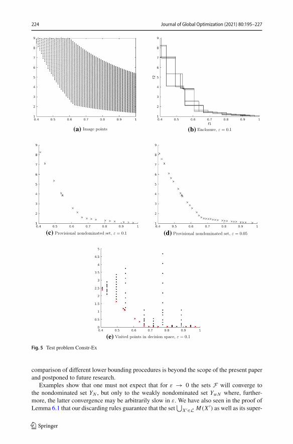
224 Journal of Global Optimization (2021) 80:195–227
(a) (b)
(c)
(e)
(d)
Fig. 5 Test problem Constr-Ex
comparison of different lower bounding procedures is beyond the scope of the present paperand postponed to future research.
Examples show that one must not expect that for ε → 0 the sets F will converge tothe nondominated set YN , but only to the weakly nondominated set YwN where, further-more, the latter convergence may be arbitrarily slow in ε. We have also seen in the proof ofLemma 6.1 that our discarding rules guarantee that the set
⋃X ′∈L M(X ′) as well as its super-
123
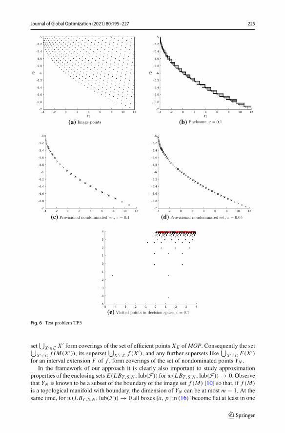
Journal of Global Optimization (2021) 80:195–227 225
(a) (b)
(c)
(e)
(d)
Fig. 6 Test problem TP5
set⋃
X ′∈L X ′ form coverings of the set of efficient points XE ofMOP. Consequently the set⋃X ′∈L f (M(X ′)), its superset
⋃X ′∈L f (X ′), and any further supersets like
⋃X ′∈L F(X ′)
for an interval extension F of f , form coverings of the set of nondominated points YN .In the framework of our approach it is clearly also important to study approximation
properties of the enclosing sets E(LBT ,S,N , lub(F)) forw(LBT ,S,N , lub(F)) → 0. Observethat YN is known to be a subset of the boundary of the image set f (M) [10] so that, if f (M)
is a topological manifold with boundary, the dimension of YN can be at most m − 1. At thesame time, for w(LBT ,S,N , lub(F)) → 0 all boxes [a, p] in (16) ‘become flat at least in one
123
226 Journal of Global Optimization (2021) 80:195–227
direction’ and thus at most (m − 1)-dimensional. This fits well to the expected dimension ofYN .
However, in general one may not expect that the enclosures E(LBT ,S,N , lub(F)) uni-formly approximate the nondominated set YN for w(LBT ,S,N , lub(F)) → 0. This is duetheir different connectedness structure. In fact, examples like Test Problem 9.2 and Test Prob-lem 9.3 show that, as opposed to the convex case [10], in the nonconvex case the set YN maybe disconnected while E(LBT ,S,N , lub(F)) is connected.
One way to construct a subset of E(LBT ,S,N , lub(F))with the same connectedness struc-ture as YN may be to intersect it with the above union of interval enclosures
⋃
X ′∈LF(X ′) ⊇ YN
for sufficiently small boxes F(X ′), X ′ ∈ L. However, in our framework this is not desirableas we wish to avoid the effort of constructing such small boxes in the first place.
Wewould also like tomention that our branch-and-bound framework can be generalized tothe presence of equality constraints in the description of the feasible set ofMOP. The crucialmodifications for this are appropriate generalizations of the lower bounding procedures aswell as meeting Assumption 8.3 for the convergence proof. As the details of this are mainlytechnical, we did not include them in the present paper for the clarity of presentation.
Acknowledgements Open Access funding enabled and organized by Projekt DEAL. The authors wish tothank the two anonymous referees and Anne-Sophie Reichhardt for their valuable comments and remarks onan earlier version of this manuscript.
Data Availability Statement Data sharing not applicable to this article as no datasets were generated oranalysed during the current study.
Open Access This article is licensed under a Creative Commons Attribution 4.0 International License, whichpermits use, sharing, adaptation, distribution and reproduction in any medium or format, as long as you giveappropriate credit to the original author(s) and the source, provide a link to the Creative Commons licence,and indicate if changes were made. The images or other third party material in this article are included in thearticle’s Creative Commons licence, unless indicated otherwise in a credit line to the material. If material isnot included in the article’s Creative Commons licence and your intended use is not permitted by statutoryregulation or exceeds the permitted use, you will need to obtain permission directly from the copyright holder.To view a copy of this licence, visit http://creativecommons.org/licenses/by/4.0/.
References
1. Adjiman, C.S., Dallwig, S., Floudas, C.A., Neumaier, A.: A global optimization method, aBB, for generaltwice-differentiable constrained NLPs: I. Theoretical advances. Comput. Chem. Eng. 22, 1137–1158(1998)
2. Al-Khayyal, F.A., Falk, J.E.: Jointly constrained biconvex programming. Math. Oper. Res. 8, 273–286(1983)
3. Androulakis, I.P., Maranas, C.D., Floudas, C.A.: αBB: a global optimization method for general con-strainted nonconvex problems. J. Glob. Optim. 7, 337–363 (1995)
4. Belotti, P.: Disjunctive cuts for nonconvex MINLP. In: Lee, J., Leyffer, S. (eds.) Mixed Integer NonlinearProgramming, pp. 117–144. Springer, Berlin (2012)
5. Binh, T.: A multiobjective evolutionary algorithm: the study cases. In: Proceedings of the 1999 Geneticand Evolutionary Computation Conference, pp 127–128 (1999)
6. Branke, J., Deb, K., Dierolf, H., Osswald, M.: Finding knees in multi-objective optimization. In: ParallelProblem Solving from Nature: PPSN VIII, Springer, pp 722–731 (2004)
7. Chen, G., Huang, X., Yang, X.: Vector Optimization. Springer, Berlin (2005)
123
Journal of Global Optimization (2021) 80:195–227 227
8. Dächert, K., Klamroth, K., Lacour, R., Vanderpooten, D.: Efficient computation of the search region inmulti-objective optimization. Eur. J. Oper. Res. 260, 841–855 (2017)
9. Deb, K.: Multi-objective optimization using evolutionary algorithms. Wiley, New York (2001)10. Ehrgott, M.: Multicriteria Optimization. Springer, Berlin (2005)11. Evtushenko, YuG, Posypkin, M.A.: Method of non-uniform coverages to solve the multicriteria optimiza-
tion problems with guaranteed accuracy. Autom. Remote Control 75, 1025–1040 (2014)12. Fernández, J., Tóth, B.: Obtaining the efficient set of nonlinear biobjective optimization problems via
interval branch-and-bound methods. Comput. Optim. Appl. 42, 393–419 (2009)13. Fonseca, C.A., Fleming, P.J.: Multiobjective genetic algorithms made easy: selection sharing and mating
restriction. In: Proceedings of the 1st International Conference on Genetic Algorithms in EngineeringSystems: Innovations and Applications, pp 45–52. IEEE Press, Piscataway, NJ (1995)
14. Füllner, C., Kirst, P., Stein, O.: Convergent upper bounds in global minimization with nonlinear equalityconstraints. Math. Program. (2020). https://doi.org/10.1007/s10107-020-01493-2
15. Gerth (Tammer), C., Weidner, P.: Nonconvex separation theorems and some applications in vector opti-mization. J. Optim. Theory Appl. 67, 97–320 (1990)
16. Göpfert, A., Riahi, H., Tammer, C., Zalinescu, C.: Variational Methods in Partially Ordered Spaces. CMSBooks. Springer, New York (2003)
17. Günther, C., Popovici, N.: New algorithms for discrete vector optimization based on the Graef–Younesmethod and cone-monotone sorting functions. Optimization 67, 975–1003 (2018)
18. Hansen, E., Walster, G.W.: Global Optimization Using Interval Analysis. Marcel Dekker Inc., New York(2004)
19. Jahn, J., Rathje, U.: Graef–Younes method with backward iteration. In: Küfer, K.-H., et al. (eds.) Mul-ticriteria Decision Making and Fuzzy Systems-Theory. Methods and Applications, pp. 75–81. Shaker,Aachen (2006)
20. Kirst, P., Stein, O., Steuermann, P.: Deterministic upper bounds for spatial branch-and-bound methods inglobal minimization with nonconvex constraints. TOP 23, 591–616 (2015)
21. Klamroth, K.: Personal communication (2017)22. Klamroth, K., Lacour, R., Vanderpooten, D.: On the representation of the search region in multi-objective
optimization. Eur. J. Oper. Res. 245, 767–778 (2015)23. Loridan, P.: ε-solutions in vector minimization problems. J. Optim. Theory Appl. 43, 265–276 (1984)24. McCormick, G.P.: Computability of gobal solutions to factorable nonconvex programs: part I—convex
underestimating problems. Math. Program. 10, 147–175 (1976)25. Miettinen, K.: Nonlinear Multiobjective Optimization. Springer, Berlin (1998)26. Niebling, J., Eichfelder, G.: A branch-and-bound based algorithm for nonconvex optimization problems.
SIAM J. Optim. 29, 794–821 (2019)27. Neumaier,A.: IntervalMethods for Systems of Equations. CambridgeUniversity Press, Cambridge (1990)28. Pardalos, P., Žilinskas, A., Žilinskas, J.: Non-convex Multi-Objective Optimization. Springer, Berlin
(2017)29. Rump, S.M.: INTLAB-interval laboratory. In: Csendes, T. (ed.) Developments in Reliable Computing,
pp 77–104. Springer, Dordrecht (1999)30. Ruzika, S., Wiecek, M.M.: Approximation methods in multiobjective programming. J. Optim. Theory
Appl. 126, 473–501 (2005)31. Scholz, D.: The multicriteria big cube small cube method. TOP 18, 286–302 (2010)32. Sawaragi, Y., Nakayama, H., Tanino, T.: Theory of Multiobjective Optimization. Elsevier, Amsterdam
(1985)33. Smith, E., Pantelides, C.: Global optimisation of nonconvex MINLPs. Comput. Chem. Eng. 21, 791–796
(1997)34. Smith, E., Pantelides, C.: A symbolic reformulation/spatial branch-and-bound algorithm for the global
optimisation of nonconvex MINLPs. Comput. Chem. Eng. 23, 457–478 (1999)35. Tawarmalani,M., Sahinidis, N.V.: Convexification andGlobal Optimization in ContinuousMixed-Integer
Nonlinear Programming. Springer, Dordrecht (2002)36. Žilinskas, A.: On the worst-case optimal multi-objective global optimization. Optim. Lett. 7, 1921–1928
(2013)37. Žilinskas, A., Žilinskas, J.: Adaptation of a one-step worst-case optimal univariate algorithm of bi-
objective Lipschitz optimization to multidimensional problems. Commun. Nonlinear Sci. Numer. Simul.21, 89–98 (2015)
Publisher’s Note Springer Nature remains neutral with regard to jurisdictional claims in published maps andinstitutional affiliations.
123