A General Framework fFor Error Analysis iIn …good/papers/408.pdf · A General Framework fFor Error Analysis iIn Measurement-Bbased GIS, ... errors in indirect measurements, a geodetic

A general framework for error analysis in measurement-based GIS ------Part 1

1

A General Framework fFor Error Analysis iIn Measurement-Bbased

GIS, Part 1: The Basic Measurement-Error Model aAnd Related Concepts

Yee Leung Department of Geography and Resource Management, Center for Environmental Policy

and Resource Management, and Joint Laboratory for Geoinformation Science, The Chinese University of Hong Kong, Hong Kong

E-mail: [email protected]

Jiang-Hong Ma Faculty of Science, Xi’an Jiaotong University and Chang’an University, Xi’an, P.R. China

E-mail: [email protected]

Michael F. Goodchild Department of Geography, University of California, Santa Barbara, California, U.S.A.

E-mail: [email protected] Abstract. This is the first part of our four-part series of papers which proposes a general framework

for error analysis in measurement-based geographical information systems (MBGIS). The purpose of

the series is to investigate the fundamental issues involved in measurement error (ME) analysis in

MBGIS, and to provide a unified and effective treatment of errors and their propagations in various

interrelated GIS and spatial operations. Part 1 deals with the formulation of the basic ME model

together with the law of error propagation. Part 2 investigates the classic point-in-polygon problem

under ME. Continued onto Part 3 is the analysis of ME in intersections and polygon overlays. In Part

4, error analyses in length and area measurements are made. In the present part, a simple but general

model for ME in MBGIS is introduced. An approximate law of error propagation is then formulated.

A simple, unified, and effective treatment of error bands for a line segment is made under the name of

“covariance-based error band”. A new concept, called “maximal allowable limit”, which guarantees

invariance in topology or geometric-property of a polygon under ME is also advanced. To handle

errors in indirect measurements, a geodetic model for MBGIS is proposed and its error distribution

problem is studied on the basis of the basic ME model as well as the approximate law of error

propagation. Simulation experiments all substantiate the effectiveness of the proposed theoretical

construct.

Keywords: Covariance-based error band, error propagation, geodetic model, geographical information

systems, maximal allowable limit, measurement error

1. Introduction Geographical information science in general and geographical information system (GIS) in

particular have developed into a major discipline that fosters theoretical investigations and practical

Comment [v1]: “Propagation” may be more suitable


2

tools for the management, analysis and display of spatial information. With the ever increasing volume

of geo-referenced data being generated, transferred, and utilized, the amount of uncertainty embedded

in spatial databases has become a major issue of crucial theoretical importance and practical

consideration. It is apparent that the oblivious use of error-laden spatial data without considering the

intrinsic uncertainty involved will lead to serious consequences in concepts and practices.

Uncertainty (in attribute values and in positions) in spatial databases generally involves accuracy,

statistical precision, and bias in initial values or in the estimated coefficients in statistically calibrated

equations. Most importantly, spatial uncertainty includes the estimation of errors (both in position and

in attribute) in the final output that result from the propagation of external (initial value) uncertainty

and internal (model) uncertainty.

Therefore, research on uncertainty in spatial data intends to investigate how uncertainties arise and

distribute through GIS operations, and to assess the plausible effects on subsequent decision-making.

It is thus important to be able to track the occurrence and propagation of uncertainties (Goodchild,

1991; UCGIS, 1996). Apparently, map accuracy is closely related to spatial uncertainty, and its

assessment and provision are essential to end users (Keefer et al., 1991). Research on accuracy must

be associated with errors in GIS. Thus the study of errors in GIS has been extensive and diverse (see

for example, Goodchild and Gopal, 1989; Leung and Yan, 1998; Mowrer and Congalton, 2000;

Stanislawski et al., 1996; Veregin, 1989; Wolf and Ghilani, 1997; Zhang and Goodchild, 2002). In a

broader context, a study in spatial statistical analysis is given in by Cressie (1993). The error

taxonomy recognizes that different classes of spatial data exhibit different types of errors, and errors

may be introduced and propagated in various stages of data manipulation and spatial processing.

Errors in spatial databases are complex and multivariate. They can generally be reckoned as

the inherent error and the operational error. Inherent error is the error present in source documents,

including the accumulated error in the map used as input to a GIS. Operational error, categorized as

positional and identification errors, is produced through the data capture and manipulation functions of

a GIS or is introduced during the process of data entry and occurs throughout data manipulation and

spatial modeling. Digitizing, for example, is one mechanism of data input that introduces error into


3

maps. Its magnitude and impact upon digital map accuracy has not been well studied (Chrisman,

1982). In fact, it is often overlooked or assumed to be negligible.

Since GIS databases, at the most general level, are based on a model of geographical data, errors

can be classified into spatial, temporal and thematic error. From the modeling point of view, they can

also be classified as either systematic or random. Systematic errors usually follow physical laws and

they can be removed by model modification. It is however impossible to avoid random errors in

measurements entirely (Wolf and Ghilani, 1997). Such random error is also called measurement error

(ME), which is one of the most important problems in the use of geo-referenced data.

It should be noted that a feature of conventional vector-based data is the representation of position

by derived coordinates, rather than by original measurements. In such coordinate-based GIS, an

important problem is the determination of error structures of location coordinates. It is a basis of error

analysis. If it is unable tocannot be solved, it will then be impossible to perform error propagation or to

estimate uncertainties in derived products. To overcome the difficulties in uncertainty management

intrinsic to conventional GIS, the concept of a measurement-based GIS (MBGIS) has been proposed

in by Goodchild (1999). Under this concept, a MBGIS is a system that provides access to

measurements used to determine the locations of objects, to the geographical procedures

(transformation functions) that link measurements to quantities to be measured, and to the rules used

to determine interpolated positions. It also provides access to the locations which may either be stored,

or derived on the fly. The basic idea is to retain details of measurements so that error analysis can be

made possible, and corrections to positions can be appropriately propagated through the database.

To make MBGIS a reality, it is essential to develop a general framework within which a rigorous

approach, particularly the statistical approach, to measurement error analysis and error propagation

can be formulated. By extendingExtended on the theory of ME (Neuilly and CETAMA, 1999) and its

analysis in the context of GIS (Heuvelink, 1998; Heuvelink et al., 1989), we propose in the present

study a formal basis for estimating how errors in a location can be propagated through various GIS

operations, and how errors in the corresponding products can be estimated.


4

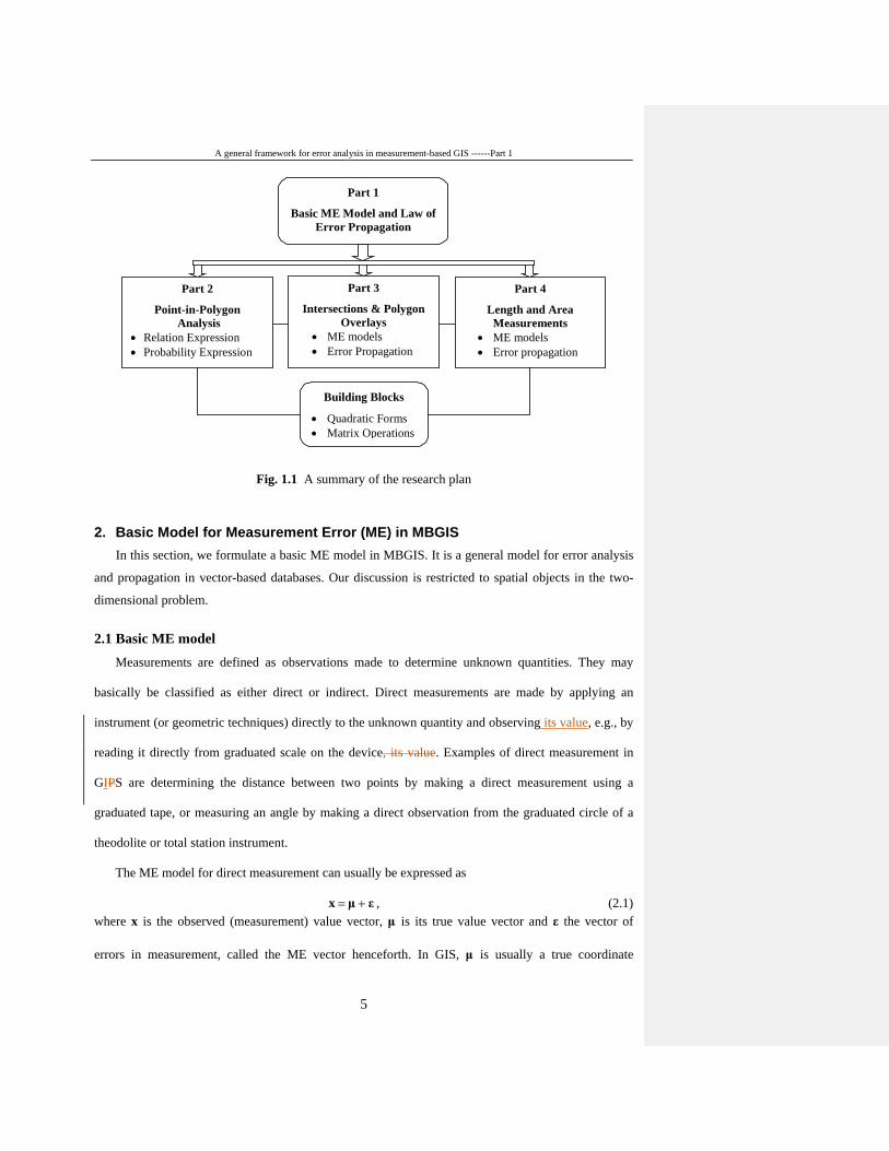
Our research work is organized into four parts (see Fig. 1.1). The purpose of this four-part series

of papers is to explore the fundamental issues involved in error analysis in MBGIS, and to render a

consistent and effective treatment of errors and their propagations in a variety of interrelated GIS and

spatial operations. We formulate in Part 1 a basic measurement error model on which formal analysis

of error propagation can be made, and ME models for various GIS operations can be constructed. On

the basis of the basic ME model, we also scrutinize the concepts of error band for a line segment, and

propose a new error-band construct, and together with a concept of maximal allowable limit for

positional error. To be able to analyze geodetic problems, a geodetic model for MBGIS is also

constructed and substantiated by numerical examples. In Part 2, we investigate the classic point-in-

polygon problem with a new perspective. We propose conditions under which the problem should be

addressed and re-open the issue of the error band for a line segment with a new view point. To make

point-in-polygon analysis under ME operable, we formulate an algebra-based probability model that

can compute probabilities by circumventing the difficulties and complexities of the geometric methods

that deal with polygons directly. In Part 3, we examine the problems surrounding line-in-polygon and

polygon-on-polygon overlays. We first formulate an approximate law for error propagation in

intersection coordinates which forms the basis for the analysis of error propagation in polygon

overlays. To further extend the scope of our analysis, we analyze in Part 4 the relative errors in length

and area measurements in MBGIS. In addition to the substantiation by numerical examples, we derive

the approximate law of error propagation in length measurements and the exact law of error

propagation in area measurements.

In what remains in this part of the four-part series, we first formulate the basic measurement error

model in MBGIS, and examine the concept of the error band for a line segment in Section 2. A

geodetic model for MBGIS is then proposed in Section 3, with a substantiation by through three

applications. We then conclude Part 1 with a summary and a prelude to Part 2.

Comment [v2]: we have not done this


5

Part 1

Basic ME Model and Law of Error Propagation

Part 4

Length and Area Measurements

• ME models • Error propagation

Part 2

Point-in-Polygon Analysis

• Relation Expression • Probability Expression

Part 3

Intersections & Polygon Overlays

• ME models • Error Propagation

Building Blocks

• Quadratic Forms • Matrix Operations

Fig. 1.1 A summary of the research plan

2. Basic Model for Measurement Error (ME) in MBGIS In this section, we formulate a basic ME model in MBGIS. It is a general model for error analysis

and propagation in vector-based databases. Our discussion is restricted to spatial objects in the two-

dimensional problem.

2.1 Basic ME model

Measurements are defined as observations made to determine unknown quantities. They may

basically be classified as either direct or indirect. Direct measurements are made by applying an

instrument (or geometric techniques) directly to the unknown quantity and observing its value, e.g., by

reading it directly from graduated scale on the device, its value. Examples of direct measurement in

GIPS are determining the distance between two points by making a direct measurement using a

graduated tape, or measuring an angle by making a direct observation from the graduated circle of a

theodolite or total station instrument.

The ME model for direct measurement can usually be expressed as

εμx += , (2.1) where x is the observed (measurement) value vector, μ is its true value vector and ε the vector of

errors in measurement, called the ME vector henceforth. In GIS, μ is usually a true coordinate


6

representation of a location, while x is the measured coordinates of the location. Indirect

measurements are obtained when it is difficult or impossible to make direct measurements. Under such

a situation, the quantity desired is determined from its mathematical (functional) relationship to direct

measurements. During this procedure, the errors that were present in the original direct observations

are distributed by the computational process into the indirect values. As a result, indirect

measurements contain errors that are functions of the original errors. This distribution of errors from

direct measurements is called error propagation (Wolf and Ghilani, 1997).

Interpolation of locations of spatial objects can be viewed as indirect measurement. A location y

may be interpolated between measured locations. Indirect measurements occur, for example, when the

position of some feature recognizable on an aerial photograph is established with respect to registered

tics or control points. They also occur when a surveyor establishes the location of a boundary by

linking surveyed monuments with a mathematical straight line.

In general, we can eliminate systematic errors which follow physical laws. So, it is reasonable to

assume that only random errors remain in the direct observations. In MBGIS, we essentially need to

derive the basic propagation equation for random errors.

Let x pR∈ be the set of p measurements which can be measured directly, y qR∈ be q required

quantities to be measured, and f (a well-defined geographical procedure, called the operation function,

or, more generally, the transformation function) be the function linking these measurements x to the

quantities y so that

)(xy f= . Once x is measured and f is known, y and the associated error distribution are uniquely and

automatically determined. The inverse of f is denoted by 1−f , that is, the function that allows

measurements x to be determined from the quantities y. This reciprocal relationship between x and y

will prove to be instrumental in error analysis and database maintenance. The basic ME model for

indirect measurement can simply be expressed as

)(XY f= , (2.2)

xx εμX += , ) ,(~ xx Σ0ε , (2.3) :)I(

Formatted


7

where xμ is the true-value vector, X the random measurement-value vector, Y the indirect

measurement-value vector obtained by f, and xε the random ME vector with zero mean 0 and the

variance-covariance matrix xΣ . To simplify, the variance-covariance matrix will be called the

covariance matrix henceforth. According to (2.2), Y is random and its error covariance matrix yΣ is

propagated from xΣ . However, it should be noted that in general yΣ also depends on the true-value

vector xμ . To see it, model (I) can be expressed as

yyxxyxxxx fEff εμεμεεμεμXY +=+++=+== )()]([ )()( , where )]([ xxy fE εμμ +≡ is dependent on xε through the expectation, and )( xxyy εμεε +≡ is

dependent on xε through a function ) ( ⋅yε . Therefore, the dependence of yμ on xε is weaker than

that of yε . Although such dependence does not occur in most cases, it should not be omitted in the

general sense. Since yΣ )cov( yε≡ )](cov[ xxy εμε += , it is often a general function of xΣ and xμ ,

i.e., yΣ );( xxF μΣ= and is dependent on xμ . In particular, when )(xf is linear in x, i.e.,

xBax )( +=f , where a and B are a constant vector and matrix respectively, we have xy μBaμ += ,

xy εBε = , and yΣ T BΣB x= .

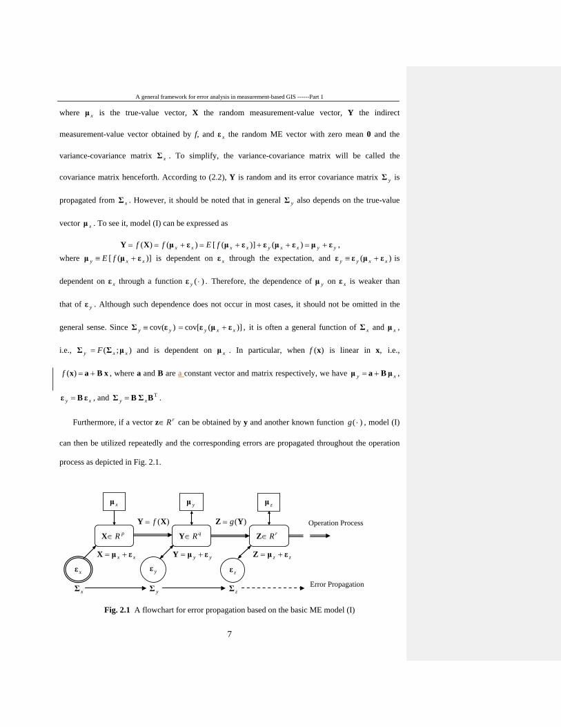
Furthermore, if a vector z rR∈ can be obtained by y and another known function ) ( ⋅g , model (I)

can then be utilized repeatedly and the corresponding errors are propagated throughout the operation

process as depicted in Fig. 2.1.

)(XY f= )(YZ g= xx εμX += yy εμY += zz εμZ += xΣ yΣ zΣ

Fig. 2.1 A flowchart for error propagation based on the basic ME model (I)

xμ yμ

xε yε

X pR∈

zμ

zε

Y qR∈ Z rR∈

Operation Process

Error Propagation


8

2.2 Approximate law of error propagation

When the transformation function )(xy f= is completely known, error propagation can

theoretically be determined in terms of this functional relationship. In this case, we can divide it

intoconsider two situations: (1) the error distribution of Y can be derived exactly from the relationship

)(XY f= , e.g., the area measurement of a triangle discussed in Leung et al. (2003d); and (2) the error

distribution cannot be exactly obtained or it is too complex to be derived because of nonlinearity of f.

In practice, the latter situation often occurs. The focus of this subsection is to derive an approximate

law of error propagation.

In case of nonlinearity, the basic idea generally adopted is to seek a linear (or second-order)

approximation to )(xy f= . First and second order Taylor methods, for example, may be analytical

approaches to solve problems in GIS. Rosenblueth’s method, on the other hand, may be an alternative

to the first- order Taylor method. If analytical expressions are not a concern, a Monte Carlo method

may be employed for easy implementation. (see Heuvelink, 1998 for a discussion).

For its analytical clarity and general applicability, we first employ the Taylor method to derive a

general approximate equation for error propagation. Consider a transformation function )(xfy = in p

variables pp Rxx ∈= T

1 ),,( x , where Ry ∈ . If this function has continuous derivatives up to (n+1)-

order, then it can be expanded into a Taylor series about a point =a pp Raa ∈T

1 ),,( as:

n

n

jaxax

p

jp

k kkkp Rxxf

xax

jxxff

pp

+

′′

′∂∂

−== ∑ ∑=

=′=′=0

,,

11

1

11

),,(

)(!

1),,()(

x , (2.4)

where nR is, called the remainder after n+1 terms. So the first-order approximation of )(xf is

∑= =′=′

′∂

′′∂−+==

p

k axaxk

pkkpp

ppx

xxfaxaafxxff

1 ,,

111

11

),,()(),,(),,(~)(~

x ,

or xbx aacf +=)(~ , (2.5)

where ∑= =′=′

′∂

′′∂−≡

m

k axaxk

pkpa

ppx

xxfaaafc

1 ,,

11

11

),,(),,(

, (2.6)

Comment [M F3]: Shouldn’t linear be first-order (constant is zero-order)? Or are you saying “linear (first-order) or second-order”?


9

pp axaxp

pp

pa x

xxf

x

xxf

=′=′×

′∂

′′∂

′∂

′′∂≡

,,

1

1

1

111

),,(,,

),,(

b . (2.7)

Iit should be noted that ca in (2.6) is a constant and ba in (2.7) is a constant matrix, and they are

independent of x. Since (2.5) is an approximation to )(xfy = , we have

xb aacy +≈ . (2.8) If we consider )(xy f= , i.e., q functions )(xii fy = in x ),,1( qi = which are approximated by

the first-order Taylor expansion (2.5), then we can express them into a vector-matrix form as:

xb iaiai cy , , +≈ , qi ,,1= , i.e., xb

b

,

1,

,

1,1

+

≈

qa

a

qa

a

q c

c

y

y , (2.9)

or xBcy aa +≈ , (2.10)

where T1 ),,( qyy =y , T

,1, ),,( qaaa cc =c , and the coefficient matrix

pp axaxj

piqaa

pqa x

xxf

=′=′×

′∂

′′∂=≡

,,

1TT,

T1,

11

),,(),,(

bbB (2.11)

is called a Jacobian matrix, which is a matrix of partial derivatives with respect to each of the

components (For simplicity and without confusion, we henceforth use iy for both the singular and

plural form of iy , (i.e., rather than using iy ’s for plural), and the same applies to all other relevant

symbols).

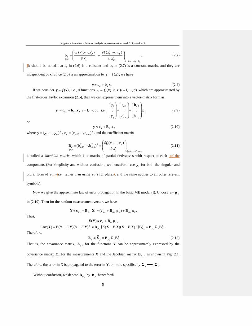
Now we give the approximate law of error propagation in the basic ME model (I). Choose xμa =

in (2.10). Then for the random measurement vector, we have

XBcY xx µµ +≈ xx xxx

εBμBc ) ( µµµ ++= . Thus,

xaaE μBcY )( +≈ , TTTT ]) )( ([ ) )( ()(Cov

xxxx xEEEEEE µµµµ BΣBBXXXXBYYYYY =−−≈−−= . Therefore,

T~xx xyy µµ BΣBΣΣ ≡≈ . (2.12)

That is, the covariance matrix, yΣ , for the functions Y can be approximately expressed by the

covariance matrix xΣ for the measurements X and the Jacobian matrix xµB , as shown in Fig. 2.1.

Therefore, the error in X is propagated to the error in Y, or more specifically xΣ yΣ .

Without confusion, we denote xµB by µB henceforth.


10

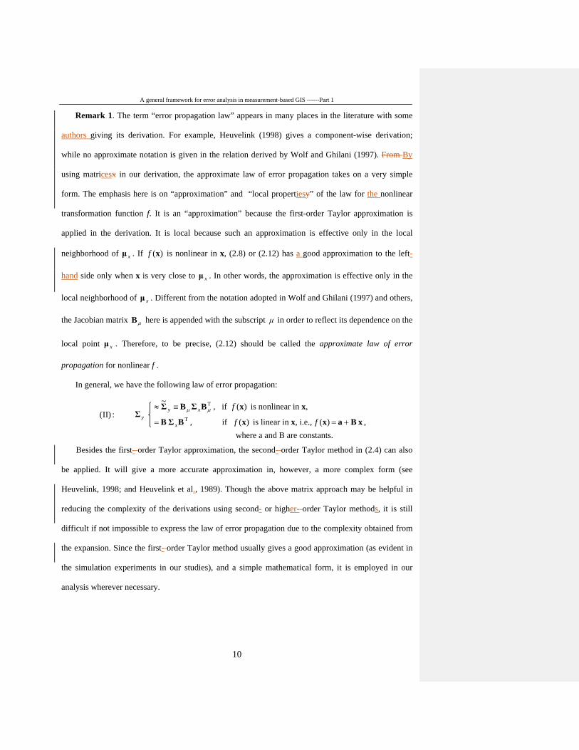
Remark 1. The term “error propagation law” appears in many places in the literature with some

authors giving its derivation. For example, Heuvelink (1998) gives a component-wise derivation;

while no approximate notation is given in the relation derived by Wolf and Ghilani (1997). From By

using matricesx in our derivation, the approximate law of error propagation takes on a very simple

form. The emphasis here is on “approximation” and “local propertiesy” of the law for the nonlinear

transformation function f. It is an “approximation” because the first-order Taylor approximation is

applied in the derivation. It is local because such an approximation is effective only in the local

neighborhood of xμ . If )(xf is nonlinear in x, (2.8) or (2.12) has a good approximation to the left-

hand side only when x is very close to xμ . In other words, the approximation is effective only in the

local neighborhood of xμ . Different from the notation adopted in Wolf and Ghilani (1997) and others,

the Jacobian matrix µB here is appended with the subscript μ in order to reflect its dependence on the

local point xμ . Therefore, to be precise, (2.12) should be called the approximate law of error

propagation for nonlinear f .

In general, we have the following law of error propagation:

T~µµ BΣBΣ xy ≡≈ , if )(xf is nonlinear in x,

T BΣB x= , if )(xf is linear in x, i.e., xBax )( +=f , where a and B are constants.

Besides the first- order Taylor approximation, the second- order Taylor method in (2.4) can also

be applied. It will give a more accurate approximation in, however, a more complex form (see

Heuvelink, 1998; and Heuvelink et al., 1989). Though the above matrix approach may be helpful in

reducing the complexity of the derivations using second- or higher- order Taylor methods, it is still

difficult if not impossible to express the law of error propagation due to the complexity obtained from

the expansion. Since the first- order Taylor method usually gives a good approximation (as evident in

the simulation experiments in our studies), and a simple mathematical form, it is employed in our

analysis wherever necessary.

:)II( yΣ


11

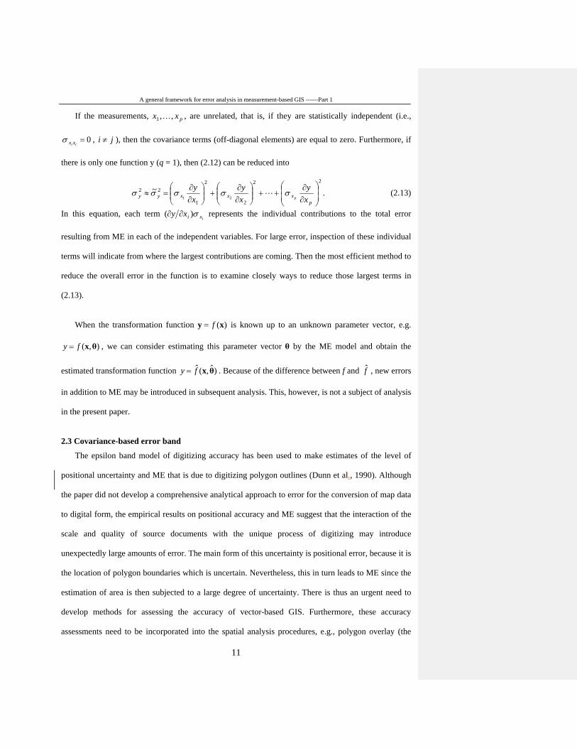
If the measurements, pxx ,,1 , are unrelated, that is, if they are statistically independent (i.e.,

0=ii xxσ , ji ≠ ), then the covariance terms (off-diagonal elements) are equal to zero. Furthermore, if

there is only one function y (q = 1), then (2.12) can be reduced into

22

2

2

1

2221

~

∂∂

++

∂∂

+

∂∂

=≈p

xxxyy xy

xy

xy

pσσσσσ . (2.13)

In this equation, each term ixixy σ)( ∂∂ represents the individual contributions to the total error

resulting from ME in each of the independent variables. For large error, inspection of these individual

terms will indicate from where the largest contributions are coming. Then the most efficient method to

reduce the overall error in the function is to examine closely ways to reduce those largest terms in

(2.13).

When the transformation function )(xy f= is known up to an unknown parameter vector, e.g.

),( θxfy = , we can consider estimating this parameter vector θ by the ME model and obtain the

estimated transformation function )ˆ,(ˆ θxfy = . Because of the difference between f and f̂ , new errors

in addition to ME may be introduced in subsequent analysis. This, however, is not a subject of analysis

in the present paper.

2.3 Covariance-based error band

The epsilon band model of digitizing accuracy has been used to make estimates of the level of

positional uncertainty and ME that is due to digitizing polygon outlines (Dunn et al., 1990). Although

the paper did not develop a comprehensive analytical approach to error for the conversion of map data

to digital form, the empirical results on positional accuracy and ME suggest that the interaction of the

scale and quality of source documents with the unique process of digitizing may introduce

unexpectedly large amounts of error. The main form of this uncertainty is positional error, because it is

the location of polygon boundaries which is uncertain. Nevertheless, this in turn leads to ME since the

estimation of area is then subjected to a large degree of uncertainty. There is thus an urgent need to

develop methods for assessing the accuracy of vector-based GIS. Furthermore, these accuracy

assessments need to be incorporated into the spatial analysis procedures, e.g., polygon overlay (the


12

sliver polygon problem) and point-in-polygon operations, used in GIS. Compared to raster-based GIS,

error analysis in vector-based GIS is much more complex.

There are a few uncertainty models for a line segment. They are for example the epsilon error

band (the commonly used buffer zone) (Perkal, 1956; Perkal, 1966; Blakemore, 1984), the error band

model (Shi, 1994; Shi et al, 1999), the σε error band and mε error band (Tong et al., 1999), and the

positional uncertainty model of line segments (Alesheikh and Li, 1996; Alesheikh et al., 1999). Some

of these concepts are either too simple for analysis or too complex in derivation. Moreover, they

usually depict a particular rather than the general version of the error band for a line segment. In fact,

the basic problems around the issue are: (a) What exactly is an error band for a line segment? (b) Can

probability be assigned to an error band? (c) What should the error band for a line segment be? We

intend to give an answer to these questions in here and Part 2 of the present series of studies.

Actually, a simple and unified error band model can be strictly established from the concept of

covariance. We call it the covariance-based error band and give its derivation and discussion as

follows:

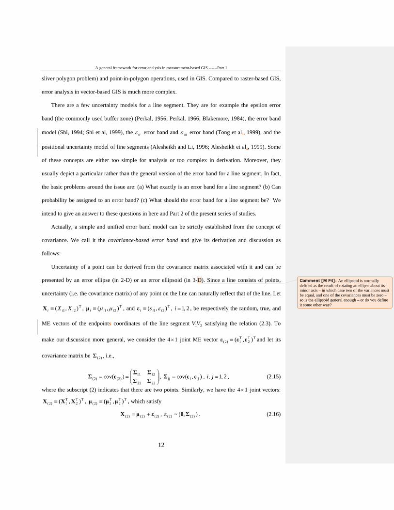
Uncertainty of a point can be derived from the covariance matrix associated with it and can be

presented by an error ellipse (in 2-D) or an error ellipsoid (in 3-D). Since a line consists of points,

uncertainty (i.e. the covariance matrix) of any point on the line can naturally reflect that of the line. Let

T21 ),( iii XX≡X , T

21 ),( iii µµ≡μ , and T21 ),( iii εε≡ε , 2 ,1=i , be respectively the random, true, and

ME vectors of the endpoints coordinates of the line segment 21VV satisfying the relation (2.3). To

make our discussion more general, we consider the 14 × joint ME vector TT2

T1)2( ),( εεε ≡ and let its

covariance matrix be )2(Σ , i.e.,

=≡

2221

1211)2()2( )cov(

ΣΣΣΣ

εΣ , ) ,cov( jiij εεΣ ≡ , 2 ,1, =ji , (2.15)

where the subscript (2) indicates that there are two points. Similarly, we have the 14 × joint vectors: TT

2T1)2( ),( XXX ≡ , TT

2T1)2( ),( μμμ ≡ , which satisfy

)2()2()2( εμX += , ),(~ )2()2( Σ0ε . (2.16)

Comment [M F4]: An ellipsoid is normally defined as the result of rotating an ellipse about its minor axis – in which case two of the variances must be equal, and one of the covariances must be zero – so is the ellipsoid general enough – or do you define it some other way?


13

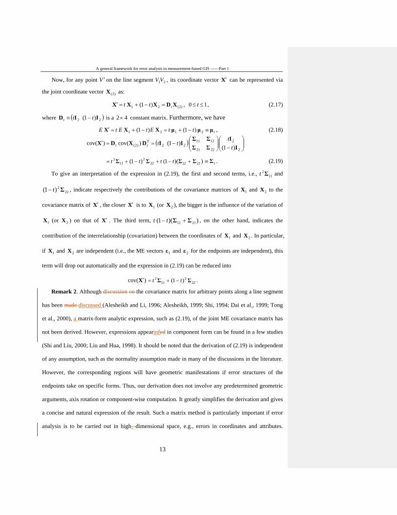
Now, for any point V ′ on the line segment 21VV , its coordinate vector X′ can be represented via

the joint coordinate vector )2(X as:

)2(21 )1( XDXXX ttt =−+=′ , 10 ≤≤ t , (2.17)

where ( )22 )1( IID ttt −≡ is a 42 × constant matrix. Furthermore, we have

2121 )1( )1( μμXXX ttEtEtE −+=−+=′ tμ≡ , (2.18)

( )

−

−==′

2

2

2221

121122

T)2( )1(

)1( )cov()cov(I

IΣΣΣΣ

IIDXDXt

ttttt

))(1( )1( 2112222

112 ΣΣΣΣ +−+−+= tttt tΣ≡ . (2.19)

To give an interpretation of the expression in (2.19), the first and second terms, i.e., 112Σt and

222)1( Σt− , indicate respectively the contributions of the covariance matrices of 1X and 2X to the

covariance matrix of X′ , the closer X′ is to 1X (or 2X ), the bigger is the influence of the variation of

1X (or 2X ) on that of X′ . The third term, ))(1( 2112 ΣΣ +− tt , on the other hand, indicates the

contribution of the interrelationship (covariation) between the coordinates of 1X and 2X . In particular,

if 1X and 2X are independent (i.e., the ME vectors 1ε and 2ε for the endpoints are independent), this

term will drop out automatically and the expression in (2.19) can be reduced into

)cov(X′ 222

112 )1( ΣΣ tt −+= .

Remark 2. Although discussion on the covariance matrix for arbitrary points along a line segment

has been made discussed (Alesheikh and Li, 1996; Alesheikh, 1999; Shi, 1994; Dai et al., 1999; Tong

et al., 2000), a matrix-form analytic expression, such as (2.19), of the joint ME covariance matrix has

not been derived. However, expressions appearinfed in component form can be found in a few studies

(Shi and Liu, 2000; Liu and Hua, 1998). It should be noted that the derivation of (2.19) is independent

of any assumption, such as the normality assumption made in many of the discussions in the literature.

However, the corresponding regions will have geometric manifestations if error structures of the

endpoints take on specific forms. Thus, our derivation does not involve any predetermined geometric

arguments, axis rotation or component-wise computation. It greatly simplifies the derivation and gives

a concise and natural expression of the result. Such a matrix method is particularly important if error

analysis is to be carried out in high- dimensional space, e.g., errors in coordinates and attributes.


14

Component-wise derivation will get to be too tedious and complicated to derive a simple and general

form for the error structure and the associated error propagation.

If we assume that )2(ε is distributed as a normal distribution, i.e., )2(ε ),0(~ )2(4 ΣN , both of 1ε

and 2ε are then normal and iii εΣε 1T − 22~ χ , 2 ,1=i , where the notation 2

pχ denotes the chi-square

distribution with p degrees of freedom. The confidence region for iμ with confidence probability

)1( α− can be constructed as:

:)({)( xVRi ≡α })()( ,),( 2,2

1TT21 αχ≤−−≡ −

iiixx μxΣμxx , 2 ,1=i , (2.20)

since αχχ ααα −=≤=≤−−=∈ −− 1][ ])()[( ])([ 2

,21T2

,21T)(

iiiiiiiiii PPRVP εΣεμXΣμXX , where 2,2 αχ

is the upper α -quantile of the chi-square distribution 22χ with 2 degrees of freedom. The shape of the

confidence region is elliptical. When =α e−1/2, this ellipse is called standard error ellipse (Alesheikh

and Li, 1996) or error ellipse (Wolf and Ghilani, 1997), which has confidence probability 0.393469.

Based on )(1

αR and )(2αR , we can construct a larger region as follows:

:)({)(}2,1{ xVR ≡α there is a real number t ( 10 ≤≤ t ) such that })()( 2

,21T

αχ≤−− −ttt μxΣμx }. (2.21)

It is obvious that )(}2,1{

αR is the union of confidence regions (ellipses) for all points on the line segment.

On this basis, we give the following definition for the error band of a line segment:

Definition 1. Assume that the joint ME vector )2(ε of the endpoints coordinates of a line segment

is normal. We call the region )(}2,1{

αR in (2.21) the covariance-based α -error band for the line segment,

henceforth notated as Cov-error band for short.

Such a band can be viewed as the confidence region for the line segment. Although its confidence

probability cannot be exactly described, simulation experiments show that it is appropriate and

effective to characterize uncertainties of a line segment (see Example 2.1). Moreover, it renders a

unified treatment of uncertainty in line segments. For example, when 2211 ΣΣ = 22

2112 IΣΣ ε=== ,

)(}2,1{

αR becomes the classical epsilon band; when 22

2211 IΣΣ σ== and =12Σ 0Σ =21 , )(}2,1{

αR

becomes the error band model. With varying )2(Σ , the Cov-error band forms varying shapes. In other

words, the Cov-error band has no fixed shape. Its shape depends on the structure of the joint ME


15

covariance matrix. This is why we can appropriately call it the Cov-error band. Therefore, the Cov-

error band in (2.21) is our answer to the question: “What exactly is an error band for a line segment? ”.

It should be noted that the confidence level of the Cov-error band is not α−1 nor 2)1( α−

although both of the confidence region )(1

αR and )(2αR for the endpoints 1μ and 2μ have confidence

level α−1 . The reason is that the random event { )(111 )( αRV ∈X and )(

222 )( αRV ∈X } is not equal to

the random event { :),( 21 XXL )(}2,1{

αR⊆ } since { )(111 )( αRV ∈X and )(

222 )( αRV ∈X } does not imply

{ 21VV )(}2,1{

αR⊆ } and vice versa, where ),( 21 XXL is the set of points on the random line segment

21VV . Thus, our answer to the question “Can probability be assigned to an error band? ” is “no” unless

a certain relaxation is made in the delimitation of the Cov-error band (to be discussed in Part 2), which

in turn becomes our answer to “What should the error band for a line segment be? ”.

Remark 3. The idea of using covariance to formulate error bands is indeed not new. Most error

band models in the literature are in one way or the other involved with the covariance matrix,

particularly Alesheikh and Li (1996) and Alesheikh et al. (1999). However, there lacks a strict and

indepth treatment that can take us through the error band problem on the basis of the covariance

matrices of the endpoints and the covariation of the endpoints is lacking.

Example 2.1 We use a numerical example to substantiate the concept of Cov-error band. Let the

true coordinate vector of the endpoints of a line segment be T1 ) 0 ,0(=μ and T

2 ) 4 ,6(=μ , and the

corresponding ME covariance matrices be respectively

=

09.0054.0054.004.0

11Σ , and

=

16.00016.0

22Σ ,

that is, 2.0,1 =σ , 3.0,2 =σ , 4.02,1, == σσ , 9.0,12 =ρ , and 012, =ρ . Here and henceforth, “,” in the

subscript is used to separate our reference to the endpoints coordinate vectors 1X and 2X . The

subscript to the left of “,” refers to the coordinate(s) of 1X and subscript to the right of “,” refers to the

coordinate(s) of 2X . For example, ,1σ means the standard deviation of the first coordinate of 1X , 2,σ

means the standard deviation of the second coordinate of 2X , and ,12ρ means the correlation

coefficient of the first and second coordinates of 2X . Fig. 2.2(a) shows the ellipses of the endpoints


16

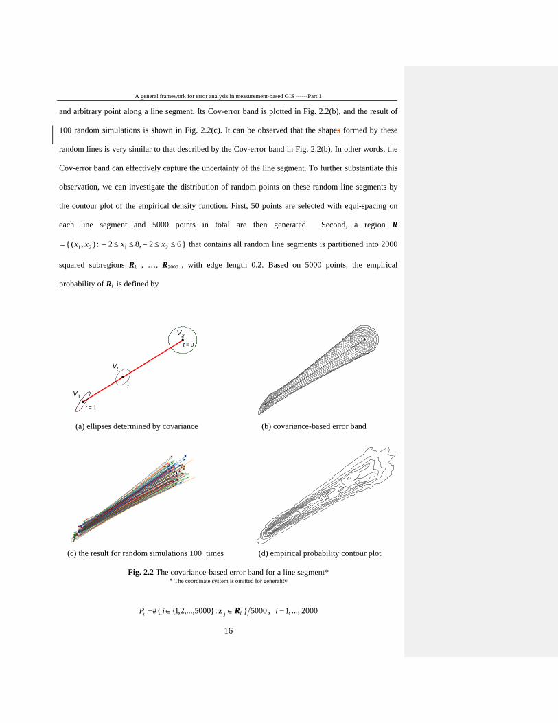
and arbitrary point along a line segment. Its Cov-error band is plotted in Fig. 2.2(b), and the result of

100 random simulations is shown in Fig. 2.2(c). It can be observed that the shapes formed by these

random lines is very similar to that described by the Cov-error band in Fig. 2.2(b). In other words, the

Cov-error band can effectively capture the uncertainty of the line segment. To further substantiate this

observation, we can investigate the distribution of random points on these random line segments by

the contour plot of the empirical density function. First, 50 points are selected with equi-spacing on

each line segment and 5000 points in total are then generated. Second, a region R

} 62 ,82 :),( { 2121 ≤≤−≤≤−= xxxx that contains all random line segments is partitioned into 2000

squared subregions R1 , …, R2000 , with edge length 0.2. Based on 5000 points, the empirical

probability of Ri is defined by

(a) ellipses determined by covariance (b) covariance-based error band

(c) the result for random simulations 100 times (d) empirical probability contour plot

Fig. 2.2 The covariance-based error band for a line segment* * The coordinate system is omitted for generality

∈∈= ji jP z:}5000,...,2,1{{# Ri 5000} , 2000 ..., ,1=i

V2

V1

t

t = 1

t = 0

Vt


17

i.e., iP is the relative frequency of the 5000 points falling into Ri . We can then plot the contour lines

of the empirical probability indicating the spatial distribution of a certain probability level (Fig.

2.2(d)). Obviously, the plot is consistent with the Cov-error band (Fig.2.2 (b)). So, the Cov-error bands

are effective in capturing the uncertainty of a line segment.

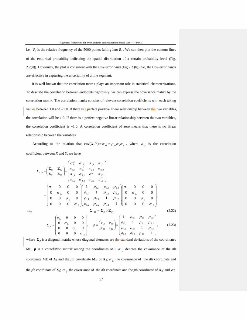
It is well known that the correlation matrix plays an important role in statistical characterizations.

To describe the correlation between endpoints rigorously, we can express the covariance matrix by the

correlation matrix. The correlation matrix consists of relevant correlation coefficients with each taking

values between 1.0 and −1.0. If there is a perfect positive linear relationship between the two variables,

the correlation will be 1.0. If there is a perfect negative linear relationship between the two variables,

the correlation coefficient is −1.0. A correlation coefficient of zero means that there is no linear

relationship between the variables.

According to the relation that yxxyxyYX σσρσ ==),cov( , where xyρ is the correlation

coefficient between X and Y, we have

=

=

22,12,2,22,1

12,21,1,21,1

2,21,22,2,12

2,11,1,122,1

2221

1211)2(

σσσσσσσσσσσσσσσσ

ΣΣΣΣ

Σ

=

2,

1,

,2

,1

12,2,22,1

12,1,21,1

2,21,2,12

2,11,1,12

2,

1,

,2

,1

000000000000

11

11

000000000000

σσ

σσ

ρρρρρρρρρρρρ

σσ

σσ

,

i.e., σσ ΣρΣΣ )2( = , (2.22)

≡

2,

1,

,2

,1

000000000000

σσ

σσ

σΣ ,

11

11

12,2,22,1

12,1,21,1

2,21,2,12

2,11,1,12

2221

1211

=

≡

ρρρρρρρρρρρρ

ρρρρ

ρ , (2.23)

where σΣ is a diagonal matrix whose diagonal elements are the standard deviations of the coordinates

ME, ρ is a correlation matrix among the coordinates ME, ji,σ denotes the covariance of the ith

coordinate ME of X1 and the jth coordinate ME of X2; ,ijσ the covariance of the ith coordinate and

the jth coordinate of X1; ij,σ the covariance of the ith coordinate and the jth coordinate of X2; and 2,iσ


18

and 2,iσ are variances of the ith coordinates of X1 and X2 respectively. For the correlation coefficients

ρ , similar notations are likewise defined.

It should be noted that both of the correlation coefficients 2,1ρ and 1,2ρ are in general not equal

since =2,1ρ ),(cor 2211 XX and =1,2ρ ),(cor 2112 XX . Thus the correlation matrix 12ρ between 1ε

and 2ε is itself not symmetric. Moreover, the correlation matrix ρ is positive semidefinite, especially,

positive definite in most cases that it is nonsingular. Although each element in ρ is a correlation

coefficient that may theoretically vary between 1 and -1, we still need to observe a restriction: the

positive semidefiniteness of ρ must be guaranteed. This case is different from that of a single

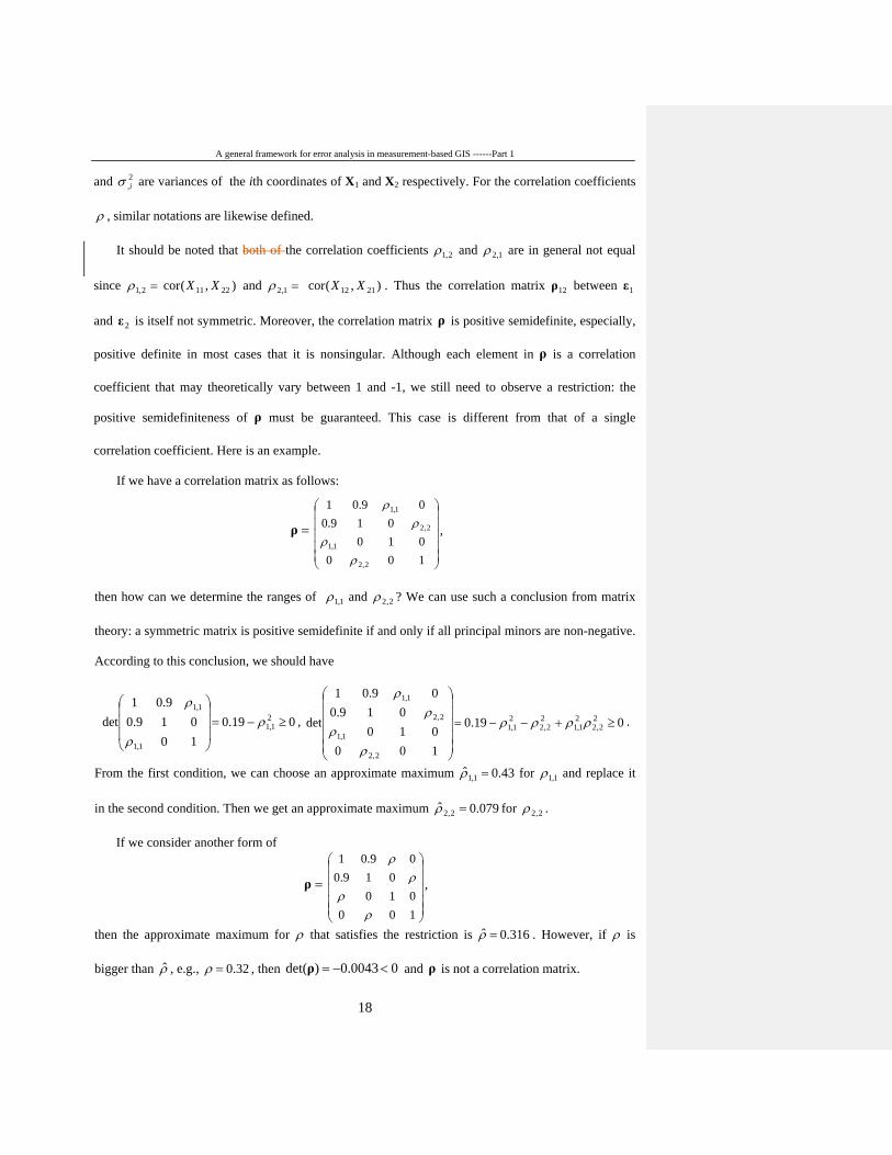
correlation coefficient. Here is an example.

If we have a correlation matrix as follows:

=ρ

100010

019.009.01

2,2

1,1

2,2

1,1

ρρ

ρρ

,

then how can we determine the ranges of 1,1ρ and 2,2ρ ? We can use such a conclusion from matrix

theory: a symmetric matrix is positive semidefinite if and only if all principal minors are non-negative.

According to this conclusion, we should have

019.010019.0

9.01det 2

1,1

1,1

1,1

≥−=

ρ

ρ

ρ, 019.0

100010

019.009.01

det 22,2

21,1

22,2

21,1

2,2

1,1

2,2

1,1

≥+−−=

ρρρρ

ρρ

ρρ

.

From the first condition, we can choose an approximate maximum 43.0ˆ 1,1 =ρ for 1,1ρ and replace it

in the second condition. Then we get an approximate maximum 079.0ˆ 2,2 =ρ for 2,2ρ .

If we consider another form of

=ρ

100010

019.009.01

ρρ

ρρ

,

then the approximate maximum for ρ that satisfies the restriction is 316.0ˆ =ρ . However, if ρ is

bigger than ρ̂ , e.g., 32.0=ρ , then 00043.0)det( <−=ρ and ρ is not a correlation matrix.


19

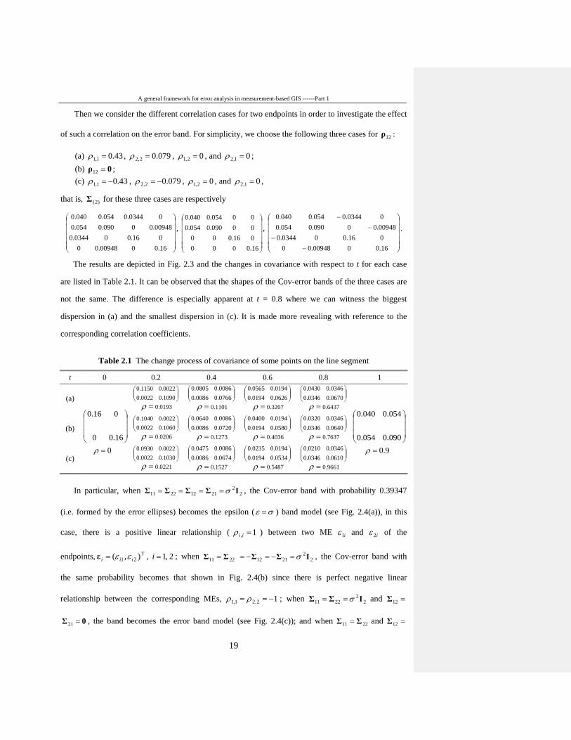
Then we consider the different correlation cases for two endpoints in order to investigate the effect

of such a correlation on the error band. For simplicity, we choose the following three cases for 12ρ :

(a) 43.01,1 =ρ , 079.02,2 =ρ , 02,1 =ρ , and 01,2 =ρ ; (b) 0ρ =12 ; (c) 43.01,1 −=ρ , 079.02,2 −=ρ , 02,1 =ρ , and 01,2 =ρ ,

that is, )2(Σ for these three cases are respectively

16.0000948.00016.000344.0

00948.00090.0054.000344.0054.0040.0

,

16.0000016.00000090.0054.000054.0040.0

,

−−

−−

16.0000948.00016.000344.000948.00090.0054.000344.0054.0040.0

.

The results are depicted in Fig. 2.3 and the changes in covariance with respect to t for each case

are listed in Table 2.1. It can be observed that the shapes of the Cov-error bands of the three cases are

not the same. The difference is especially apparent at t = 0.8 where we can witness the biggest

dispersion in (a) and the smallest dispersion in (c). It is made more revealing with reference to the

corresponding correlation coefficients.

Table 2.1 The change process of covariance of some points on the line segment

t 0 0.2 0.4 0.6 0.8 1

(a)

1090.00022.00022.01150.0

=ρ 0.0193

0766.00086.00086.00805.0

=ρ 0.1101

0626.00194.00194.00565.0

=ρ 0.3207

0670.00346.00346.00430.0

=ρ 0.6437

(b)

1060.00022.00022.01040.0

=ρ 0.0206

0720.00086.00086.00640.0

=ρ 0.1273

0580.00194.00194.00400.0

=ρ 0.4036

0640.00346.00346.00320.0

=ρ 0.7637

(c)

1030.00022.00022.00930.0

=ρ 0.0221

0674.00086.00086.00475.0

=ρ 0.1527

0534.00194.00194.00235.0

=ρ 0.5487

0610.00346.00346.00210.0

=ρ 0.9661

In particular, when 2211 ΣΣ = 22

2112 IΣΣ σ=== , the Cov-error band with probability 0.39347

(i.e. formed by the error ellipses) becomes the epsilon ( σε = ) band model (see Fig. 2.4(a)), in this

case, there is a positive linear relationship ( 1, =iiρ ) between two ME i1ε and i2ε of the

endpoints, T21 ),( iii εε=ε , 2 ,1=i ; when 2211 ΣΣ = 2

22112 IΣΣ σ=−=−= , the Cov-error band with

the same probability becomes that shown in Fig. 2.4(b) since there is perfect negative linear

relationship between the corresponding MEs, 12,21,1 −== ρρ ; when 22

2211 IΣΣ σ== and =12Σ

0Σ =21 , the band becomes the error band model (see Fig. 2.4(c)); and when 2211 ΣΣ = and =12Σ

0 16.00

016.0

=

ρ 9.0 090.0054.0

054.0040.0

=

ρ


20

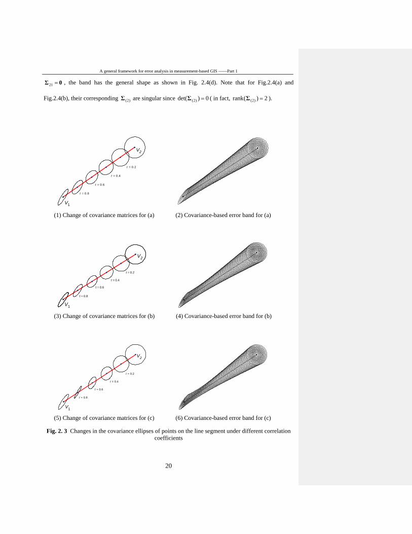
0Σ =21 , the band has the general shape as shown in Fig. 2.4(d). Note that for Fig.2.4(a) and

Fig.2.4(b), their corresponding )2(Σ are singular since 0)det( )2( =Σ ( in fact, 2)(rank )2( =Σ ).

Fig. 2. 3 Changes in the covariance ellipses of points on the line segment under different correlation

coefficients

(1) Change of covariance matrices for (a) (2) Covariance-based error band for (a) (3) Change of covariance matrices for (b) (4) Covariance-based error band for (b) (5) Change of covariance matrices for (c) (6) Covariance-based error band for (c)

V1

V2

t = 0.8

t = 0.6

t = 0.4

t = 0.2

t = 0.2

V2

t = 0.4

t = 0.6

t = 0.8

V1

V2

t = 0.2

t = 0.4

t = 0.6

t = 0.8

V1


21

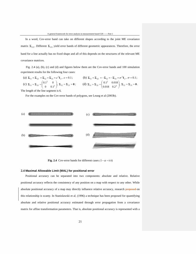
In a word, Cov-error band can take on different shapes according to the joint ME covariance

matrix )2(Σ . Different )2(Σ yield error bands of different geometric appearances. Therefore, the error

band for a line actually has no fixed shape and all of this depends on the structures of the relevant ME

covariance matrices.

Fig. 2.4 (a), (b), (c) and (d) and figures below them are the Cov-error bands and 100 simulation

experiment results for the following four cases:

(a) 2211 ΣΣ = 22

2112 IΣΣ ε=== , 1.0=ε ; (b) 2211 ΣΣ = 22

2112 IΣΣ σ=−=−= , 1.0=σ ;

(c)

== 2

2

2211 1.0001.0ΣΣ , 0ΣΣ == 2112 ; (d)

== 2

2

2211 2.0018.0018.01.0ΣΣ , 0ΣΣ == 2112 .

The length of the line segment is 6.

For the examples on the Cov-error bands of polygons, see Leung et al (2003b).

Fig. 2.4 Cov-error bands for different cases ( α−1 = 0.9) 2.4 Maximal Allowable Limit (MAL) for positional error

Positional accuracy can be separated into two components: absolute and relative. Relative

positional accuracy reflects the consistency of any position on a map with respect to any other. While

absolute positional accuracy of a map may directly influence relative accuracy, research proposed on

this relationship is scanty. In Stanislawski et al. (1996) a technique has been proposed for quantifying

absolute and relative positional accuracy estimated through error propagation from a covariance

matrix for affine transformation parameters. That is, absolute positional accuracy is represented with a

)a(

)b(

)c(

)d(


22

certainty region (propagated error ellipses) for transformed points, and relative accuracy is represented

with confidence intervals for distance and azimuth values computed between transformed points.

Since these two classes of accuracy are related, when a one class of error is investigated the other

class should be considered. It is well known that one of the important characteristics of a spatial object

is its topological (or geometrical) property which involves relative error. Although we can tolerate a

certain degree of ME in locations, ME must be restricted in a certain range so that it will not distort the

original topology. That is, it is necessary to put a limit on ME in order to guarantee that the topology

of a spatial object is invariant under ME. We call such limit the maximal allowable limit (MAL) for

ME. For example, if two points A and B are in a straight line and have a relative locational relationship

(e.g., A is the left of B), their measurements A’ and B’ may no longer maintain the original (true)

locational relationship or may even enter into an opposite relationship (e.g., A’ is to the right of B’)

due to exceedingly large ME. Such measurements are thus reality distorting. Therefore, large ME may

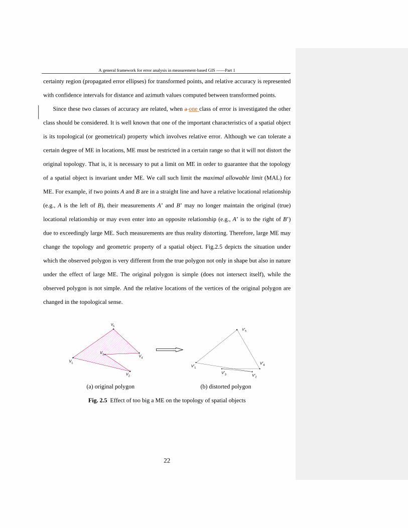
change the topology and geometric property of a spatial object. Fig.2.5 depicts the situation under

which the observed polygon is very different from the true polygon not only in shape but also in nature

under the effect of large ME. The original polygon is simple (does not intersect itself), while the

observed polygon is not simple. And the relative locations of the vertices of the original polygon are

changed in the topological sense.

V5

V4V3

V2

V1

V'1

V'5

V'3 V'2

V'4

(a) original polygon (b) distorted polygon

Fig. 2.5 Effect of too big a ME on the topology of spatial objects


23

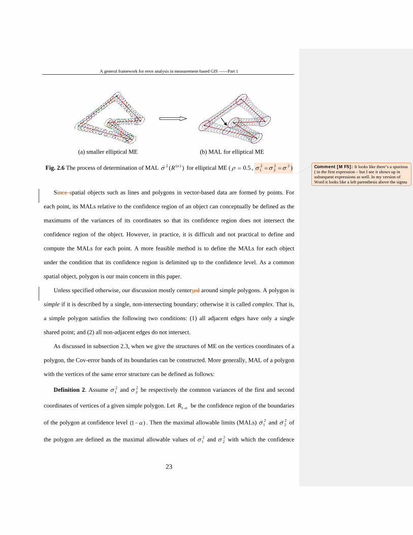
Fig. 2.6 The process of determination of MAL )( )(2 ασ R for elliptical ME ( 5.0=ρ , 22

221 σσσ == )

Since spatial objects such as lines and polygons in vector-based data are formed by points. For

each point, its MALs relative to the confidence region of an object can conceptually be defined as the

maximums of the variances of its coordinates so that its confidence region does not intersect the

confidence region of the object. However, in practice, it is difficult and not practical to define and

compute the MALs for each point. A more feasible method is to define the MALs for each object

under the condition that its confidence region is delimited up to the confidence level. As a common

spatial object, polygon is our main concern in this paper.

Unless specified otherwise, our discussion mostly centersed around simple polygons. A polygon is

simple if it is described by a single, non-intersecting boundary; otherwise it is called complex. That is,

a simple polygon satisfies the following two conditions: (1) all adjacent edges have only a single

shared point; and (2) all non-adjacent edges do not intersect.

As discussed in subsection 2.3, when we give the structures of ME on the vertices coordinates of a

polygon, the Cov-error bands of its boundaries can be constructed. More generally, MAL of a polygon

with the vertices of the same error structure can be defined as follows:

Definition 2. Assume 21σ and 2

2σ be respectively the common variances of the first and second

coordinates of vertices of a given simple polygon. Let α−1R be the confidence region of the boundaries

of the polygon at confidence level )1( α− . Then the maximal allowable limits (MALs) 21σ and 2

2σ of

the polygon are defined as the maximal allowable values of 21σ and 2

2σ with which the confidence

(a) smaller elliptical ME (b) MAL for elliptical ME

Comment [M F5]: It looks like there’s a spurious ( in the first expression – but I see it shows up in subsequent expressions as well. In my version of Word it looks like a left parenthesis above the sigma


24

region (given by α−1R ) of each vertexices does not intersect the confidence regions (bands) of its

disjoint edges, and are denoted by )( )(21

ασ R and )( )(22

ασ R .

Since a confidence level is attached to the confidence regions, we may consider it as the

confidence level of MAL.

Thus as long as the ME variances 21σ and 2

2σ are not greater than 21σ and 2

2σ respectively, the

observed polygon in the presence of ME will not change the topological property of the original (true)

polygon (i.e., the situation in Fig.2.5 will not occur) at the confidence level )1( α− and their

difference results only from errors in position of the vertices. In this definition, the confidence region

of the boundaries (line segments) of a polygon can be formed by any error bands of its edges.

According to the advantages of the Cov-error bands, we will use the Cov-error bands as a basis for the

formulation of the confidence regions of the boundaries of a polygon. Unfortunately, the confidence

level of a Cov-error band cannot be determined analytically at present. An approximation to the Cov-

error bands proposed in Leung et al (2003b) can however enables us to give a lower bound of the

confidence level.

In general, it may not be easy to determine directly the MAL. Since the shape of the confidence

region of a polygon depends on the structure of ME at the vertices, the ME structure becomes a key to

obtain MALs more easily. Under certain particular situations of ME, the determination of MALs can

indeed be simplified. For example, if all of the MEs of the vertices have positive linear relationships

and have circular ME, i.e., 22

21 ii σσ = 2σ≡ , the well-known epsilon-band is chosen (see Fig. 2.4(a))

and the corresponding MAL can be computed by distance. When 22

21 ii σσ = 2σ≡ and the correlation

coefficient ρ between 1iε and 2iε is fixed at a certain value, e.g., 0.5, the determination of MAL

using the Cov-error band is illustrated in Fig.2.6. It can be observed that the larger is the confidence

level, the wider are the Cov-error bands and the smaller are the corresponding MALs (see Leung et al

(2003b)).


25

MAL is thus a useful concept, particularly for ME simulation and modeling in order to control the

allowable range of ME. However, we may not need to consider MAL in practice if ME is sufficiently

small.

3. A geodetic model for MBGIS Based on the basic ME model (I) and error propagation law (II), we establish in this section a

geodetic model for MBGIS and substantiate it with three simple applications in geodesy.

3.1 A geodetic model for MBGIS

A MBGIS may be defined as one that provides access to the measurements m used to determine

the locations of objects, to the function f, and to the rules used to determine interpolated positions. It

also provides access to the locations, which may either be stored, or derived on the fly from

measurements.

We consider the cases that these positions are indirectly measured by an instrument and some

control points or monuments that are established with great accuracy by geodetic survey. Actually, a

MBGIS can be constructed with reference to a geodetic model, which is formulated in such a way that

locations are arranged in a hierarchy (see Fig. 3.1). At the top of the hierarchy is a small number of

control points. From these a much larger number of locations are established by measurements,

through a process of densification. Since these measurements are not as accurate as those used to

establish the monuments, the second tier of locations is also less accurately known. Further

measurements using even less accurate instruments are used to register aerial photographs, lay out

boundary lines, and determine the contents of geographic databases.

Since there will be strong correlations in errors between any locations whose lineages share part or

the entire tree, all points inherit the errors present in the monuments, but distance between points that

share the same monument are not affected by errors in the location of the monument itself. Through

the hierarchical structure of the data and the measurement methods, we can derive the law or

approximate law for error propagation at every location. Thus it is possible to analyze uncertainties in

the results of some GIS operations such as overlay and area measurement because of inaccuracies in

positioning.

Comment [M F6]: In the original paper I was careful to stress that the use of the term “geodetic” did not imply that geodesy still uses this approach – it reflects a highly simplified model of traditional surveying – it might be better to use another word, perhaps hierarchical?


26

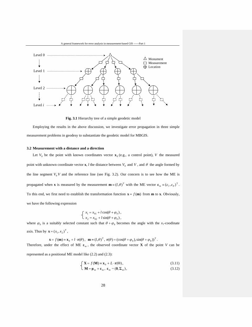
Based on the above discussion, a MBGIS can be formally structured as a hierarchy. As depicted in

Fig. 3.1, let )(ix denote the location at level i in the hierarchy. Then locations at level i+1 are derived

from locations at levels less than or equal to i through equations of the form:

),( )()()1( iii

i f xmx =+ . (3.1) The top (or root) of the tree are locations )0(x which are monuments that anchor the tree. At each level

the measurements )(im constitute the trunks, the locations to be measured are the corresponding

leaves, and the functions if are stored, and the locations )(ix are either stored or derived as needed.

For a multi-level MBGIS with different measurements and functions in various levels, the

propagation of error from the first level (can be from any level less than or equal to i through the tree)

can be carried out via the relation between )1( +ix and )(ix depicted in (3.1).

Now we establish the ME model from the root )0(x to any location )(ix and discuss its error

propagation problems. Let )(iM , )(imε and )(i

mμ be respectively the random measurement vector, the

ME vector and the true value vector of )(im , and let )(iX be the random measurement vector of )(ix ,

)cov( )()( im

im εΣ ≡ . Then, )(iM can be expressed as

)(iM += )(imμ

)(imε , ) ,(~ )()( i

mi

m Σ0ε . (3.2) Since )0(x is the monument, it can be viewed as constant without ME. For the sake of having

unified notations, we let )0()1( MM ≡ , )0(

)1( mμμ ≡ , )0()1( mεε ≡ , and )0(

)1()1( )cov( mΣεΣ =≡ . Thus we have

the ME model for )1(x :

),()( )0()0(0)1(1

)1( xMMX fg ≡= , (3.3)

)1(M += )1(μ )1(ε , ) ,(~ )1()1( Σ0ε , (3.4) which is just the basic ME model (I). So, by similar procedure, the corresponding approximate law for

error propagation can be established as:

T)1(

)1()1()1()1()1(

~)cov( µµ BΣBΣXΣ ≡≈≡ xx ,

where )1(µB is the Jacobian matrix of )( )1(1 Mg at )1(M )1(μ= .

According to (3.1) and (3.2), we can obtain the composite function 2g as follows:

)()),(,(),( )2(2)0()0(

0)1(

1)1()1(

1)2( MxMMXMX gfff === ,

:)1M.(


27

where )),(,()( )0()0(0

)1(1)2(2 xMMM ffg ≡ defined by 0f and 1f is a function of the joint ME vector

≡)2(M TT)1(T)0( ),( MM . Similarly, we can define the symbols )2(μ and )2(ε , and obtain the ME

model, like (I), for )2(x : )( )2(2

)2( MX g= , (3.5)

)2(M += )2(μ )2(ε , ) ,(~ )2()2( Σ0ε , (3.6) and the approximate law of error propagation is:

T)2(

)2()2()2()2()2(

~)cov( µµ BΣBΣXΣ ≡≈≡ xx ,

where )2(µB is the Jacobian matrix of )( )2(2 Mg at )2(M )2(μ= , )cov( )2()2( εΣ ≡ , ≡)2(ε

TT)1(T)0( ),( mm εε ,

and )(imε ( 1 ,0=i ) are defined by (3.2). The propagation relation between the error covariance matrices

)0()1( mΣΣ = and )2(Σ is given by

= )1(T

)1(),1(

)1(),1()1()2(

mm

m

ΣΣΣΣ

Σ .

Recursively, we have )),(,(),( )2()2(

2)1(

1)1()1(

1)( −−

−−

−−−

− == iii

ii

iii

i fff XMMXMX )())),(,,(,( )(

)0()0(0

)2(2

)1(1 ii

ii

ii gfff MxMMM === −

−−

− , (3.7) which results in the general ME model:

)( )()(

iii g MX = , (3.8)

)()()( iii εμM += , ) ,(~ )()( ii Σ0ε , (3.9) and

T)(

)()()()()(

~)cov(ii i

ix

iix µµ BΣBΣXΣ ≡≈≡ , (3.10)

where )( iµB is the Jacobian matrix of )( )(iig M at )(iM )(iμ= , )cov( )()( ii εΣ ≡ , ≡)(iε

TT)1(T)1( ),( −

−i

mi εε TT)1(T)2(T)0( ) ,,,( −−= i

mi

mm εεε , and )(imε ( ii , ,0 = ) are defined by (3.2). The propagation relation

between the successive error covariance matrices is given by

= −

−−

−−−)1(T

)1(),1(

)1(),1()1()( i

mimi

imiii ΣΣ

ΣΣΣ .

Obviously, both of the ME model )1M.( and )2M.( can be unified into )M.( i . The corresponding

approximate laws of error propagation can also be unified into (3.10). The models )M.( i and (3.10)

provide an effective tool for error propagation from the root )0(x to any location )(ix at level i. They

form the basis for error analysis in the geodetic model for MBGIS. Moreover, using a similar

approach, we can formulate the ME model and the approximate law of error propagation from any

location )(ix at level i to the location derived from )(ix at level higher than i.

:)2M.(

:)M.( i


28

Level 0 Monument Measurement Location Level 1 Level 2 Level i

Fig. 3.1 Hierarchy tree of a simple geodetic model

Employing the results in the above discussion, we investigate error propagation in three simple

measurement problems in geodesy to substantiate the geodetic model for MBGIS.

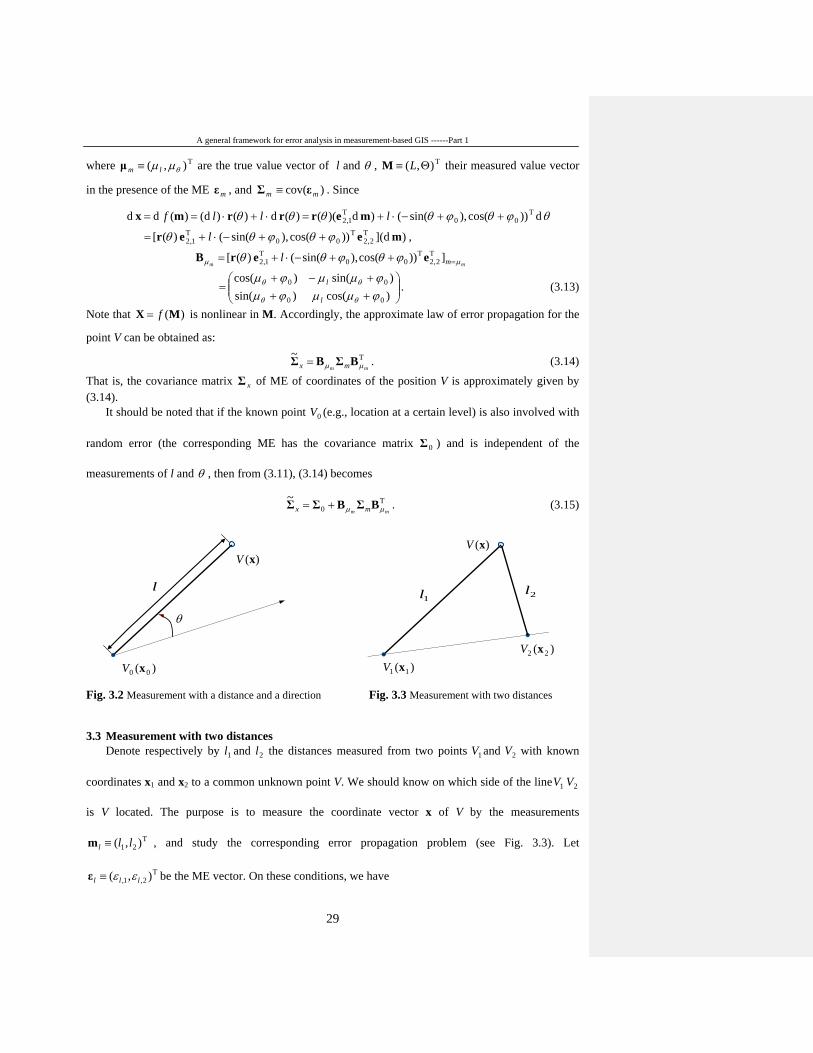
3.2 Measurement with a distance and a direction

Let 0V be the point with known coordinates vector 0x (e.g., a control point), V the measured

point with unknown coordinate vector x, l the distance between 0V and V , and θ the angle formed by

the line segment 0V V and the reference line (see Fig. 3.2). Our concern is to see how the ME is

propagated when x is measured by the measurement T),( θl≡m with the ME vector T),( θεε lm ≡ε .

To this end, we first need to establish the transformation function )(mx f= from m to x. Obviously,

we have the following expression

)cos( 0011 ϕθ ++= lxx , )sin( 0022 ϕθ ++= lxx ,

where 0ϕ is a suitably selected constant such that 0ϕθ + becomes the angle with the x1-coodinate

axis. Thus by T21 ),( xx=x ,

)()( 0 θrxmx ⋅+≡= lf , T),( θl≡m , T00 ))sin(),(cos()( ϕθϕθθ ++=r .

Therefore, under the effect of ME mε , the observed coordinate vector X of the point V can be

represented as a positional ME model like (2.2) and (2.3):

)()( 0 Θ⋅+≡= rxMX Lf , (3.11) mm εμM += , ),(~ mm Σ0ε , (3.12)


29

where T),( θµµ lm ≡μ are the true value vector of l and θ , T),( Θ≡ LM their measured value vector

in the presence of the ME mε , and mΣ )cov( mε≡ . Since

θϕθϕθθθθ d))cos(),sin(() d)(()( d)() d()( d d T00

T1,2 ++−⋅+=⋅+⋅== lllf merrrmx

) d]())cos(),sin(( )([ T2,2

T00

T1,2 meer ϕθϕθθ ++−⋅+= l ,

mm ml µµ ϕθϕθθ =++−⋅+= ]))cos(),sin(( )([ T

2,2T

00T

1,2 eerB

+++−+

=)cos()sin()sin()cos(

00

00

ϕµµϕµϕµµϕµ

θθ

θθ

l

l . (3.13)

Note that )(MX f= is nonlinear in M. Accordingly, the approximate law of error propagation for the

point V can be obtained as: T~

mm mx µµ BΣBΣ = . (3.14)

That is, the covariance matrix xΣ of ME of coordinates of the position V is approximately given by (3.14).

It should be noted that if the known point 0V (e.g., location at a certain level) is also involved with

random error (the corresponding ME has the covariance matrix 0Σ ) and is independent of the

measurements of l and θ , then from (3.11), (3.14) becomes

T0

~mm mx µµ BΣBΣΣ += . (3.15)

Fig. 3.2 Measurement with a distance and a direction Fig. 3.3 Measurement with two distances 3.3 Measurement with two distances

Denote respectively by 1l and 2l the distances measured from two points 1V and 2V with known

coordinates x1 and x2 to a common unknown point V. We should know on which side of the line 1V 2V

is V located. The purpose is to measure the coordinate vector x of V by the measurements

T21 ),( lll ≡m , and study the corresponding error propagation problem (see Fig. 3.3). Let

T2,1, ),( lll εε≡ε be the ME vector. On these conditions, we have

)(xV

)( 00 xV

θ

l

)(xV

1l 2l

)( 11 xV)( 22 xV


30

)()( T2iiil xxxx −−= , 2 ,1=i ,

which can be viewed as an equation ,(xlF ml 0) = . According to the implicit function theorem, we can

obtain the required transformation function (lf=x ml ) . Thus, the positional ME model is

)( llf MX = , (3.16) lll εμM += , ),(~ ll Σ0ε , (3.17)

where T2,1, ),( lll µµ≡μ is the true vector of lm , Ml T

21 ),( LL≡ the observed vector of lm under the

ME.

Although the explicit expression of ) ( ⋅lf is not given, the Jacobian matrix can still be obtained.

Indeed, by differentiating the above equalities, we have

) d()() (d T xxx iii ll −= , 2 ,1=i , which can be rewritten in matrix form as

(d 0

0) d(

)()(

2

1T

2

T1

=

−−

ll

xxxxx )lm , i.e., (d

00

)()( d

2

11

T2

T1

−−

=−

ll

xxxxx )lm . (3.18)

Therefore,

lµBl

ll

μxxxx

−−

=−

2

11

T2

T1

00

)()(

−−

=−

2,

1,1

T2

T1

00

)()(

l

l

x

x

μμ

xμxμ

. (3.19)

It should be noted that T2,1, ),( xxx µµ≡μ in (3.19) is determined by )()( T2

, ixixil xμxμ −−=µ ,

2 ,1=i , i.e., xμ is the true coordinate vector of the unknown point V. Accordingly, lµB is only

dependent on lμ . The approximate law for error propagation is

T~ll lx µµ BΣBΣ = . (3.20)

Fig. 3.4 An angle and two azimuths Fig. 3.5 Measurement with two angles

)( 11 xV)( 22 xV

)(xV

1θ

2x )(xV

)( 22 xV)( 11 xV

1θ 2θ


31

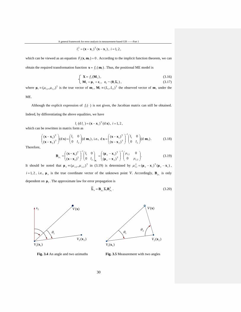
3.4 Measurement with two angles

In surveying, a useful concept is azimuths or angles. For example, the positions of widely spaced

stations can be computed from measured angles and a minimal number of measured distances called

baselines (Wolf and Ghilani, 1997). The azimuth of an object is the angular distance along the horizon

to the location of the object. By convention, azimuth is measured from north towards the east along

the horizon (see Fig. 3.4). We will utilize such a concept in order to make our conclusions suitable to

such a task.

First, we introduce an equation for angle observation. In Fig. 3.4, the azimuths of V(x) and )( 22 xV

with respect to )( 11 xV can be used to represent an angle 1θ between two line segments:

1θ Dxxxx

xxxx

VVV +

−

−−

−

−=∠≡ −−

2,12

1,111

2,12,2

1,11,2121 tantan , (3.21)

where D is a constant that depends on the quadrants in which V and 2V occur (for details, see Wolf

and Ghilani (1997)), here V and 2V correspond to the backsight and foresight station respectively, and

1V the instrument station, T2,1, ),( iii xx=x , 2 ,1=i , T

21 ),( xx=x .

Now assume that the unknown point V is measured by two angles 1θ and 2θ in 1V and 2V ,

respectively. Then for 2θ we have also the corresponding equation

2θ Dxxxx

xxxx

VVV +

−

−−

−

−=∠≡ −−

2,22,1

1,21,11

2,22

1,21121 tantan . (3.22)

They can be formed into a new multivariate equation 0),( =θθ mxF , where T21 ),( θθθ ≡m is the

measurement. Once again, the implicit function theorem can be applied. The transformation function

)( θθ mx f= is formally generated. In the presence of the ME vector T2,1, ),( θθθ εε≡ε , the positional

ME model is

)( θθ MX f= , (3.23) θθθ εμM += , ),(~ θθ Σ0ε , (3.24)

where T2,1, ),( θθθ µµ≡μ is the true vector of θm , T

21 ),( ΘΘ≡θM the observed vector of θm under

the ME θε .

Differentiating (3.21) and (3.22), and by straightforward calculation, we obtain

)(d)(d )()(d )( 12

1,12,1221,11 θxlxxxxxx =−−− ,

)(d)(d )()(d )( 22

2,21,2112,22 θxlxxxxxx =−−− ,

where )()( T2, iiixl xxxx −−= , 2 ,1=i . Solving this system for T

21 )d,d(d xx=x , we obtain


32

=x d ) (d 0

0)(

)(2

2,

21,

1

1,212,22

1,112,12θm

−−−

−−− −

x

x

ll

xxxxxxxx

.

Thus,

θ

θµ

μθ

B=

−

−−−

−−−= 2

2,

21,

1

1,212,22

1,112,12

00

)()(

x

x

ll

xxxxxxxx

( )θμθxxxx

xxxx =−−

−−= 1

22,2

21,

21)( )(

| |1

xx ll

( ))( )( | |

11

22,2

21,

21xμxμ

xμxμ−−

−−= xlxl

xxµµ , (3.25)

T~θθ µθµ BΣBΣ =x . (3.26)

Similar to (3.19), xμ in (3.25) is determined by )()( T2, ixixil xμxμ −−=µ , 2 ,1=i , where 1,lµ and

2,lµ are true edges VV1 and VV2 of the triangle formed by the edge 21VV and the two true angles 1,θµ

and 2,θµ (see Fig. 3.5).

Based on two angles 1θ and 2θ measured from known (or control) points, it has been determined

that the position of the unknown point can be uniquely determined. The propagated ME is

approximately given by (3.26). However, if additional measurement point (e.g., V3) is available, the

determination of the position of an unknown point can be strengthened by the adjustment of the least

squares method (Wolf and Ghilani, 1997). The trilateration (distance measurements) and triangulation

(angle measurements) adjustments in surveying are all performed by additional measurements.

To show the applicability of these models, we give the following simulation experiment as an

example:

Example 3.1 Suppose that two known points are )( 11 xV and )( 22 xV , T1 ) 1 ,1 (=x , T

2 ) 1 ,5 (=x ,

an unknown point V to be measured is above the line segment V1V2 , and the true position of the

unknown point V is T) 3 ,2 (=xμ . The true distances are 5)()( 1T

11, =−−= xμxμ xxlµ ,

13)()( 2T

22, =−−= xμxμ xxlµ , T) 13 ,5(=lμ . From the relation

)()( T2iiil xxxx −−= , 2 ,1=i ,

we can get for T21 ) ,( xx=x

)(3 22

218

11 llx −+= ,

21

)23232256(1 42

22

21

22

41

218

12 llllllx −⋅⋅+⋅+−⋅+−+= .


33

Thus we can obtained the transformation function )(LX f= and the ME model:

−⋅⋅+⋅+−⋅+−+

−+≡=

=

21

)23232256(1

)(3)( 4

222

21

22

41

218

1

21

218

1

2

1

LLLLLLLL

fXX

ll MX ,

+

=+=

=

2,

1,

2

1

135

l

llll L

Lεε

εμM ,

Assume that ) ,(~ 2 ll N Σ0ε , 22 IΣ σ=l , and 2.0=σ . According to (3.19) and (3.20), we have

lµBl

ll

μxxxx

−−

=−

2

11

T2

T1

00

)()(

−=

−

=−

135313252

81

13005

2321 1

,

T~ll lx µµ BΣBΣ =

=

=

03625.00025.000250.00450.0

3229

161

161

89

2σ .

To substantiate the effectiveness of xΣ~ , by 10000 random simulations we obtain the following

sample mean and sample covariance matrix

=

99164.200108.2

X , =xΣ̂

03640.000418.000418.004483.0 .

Obviously, the difference between the simulated covariance matrix xΣ̂ and the propagated covariance

matrix xΣ~ is very small. Therefore, xΣ~ can approximately represent the covariance matrix of the ME

vector of the position to be measured.

4. Conclusion

We have proposed in this part of the four-part series of papers a general framework for error

analysis in measurement-based GIS within which the basic ME model has been constructed and the

law of error propagation has been derived. A simple, strict and unified error band model for a line,

called the “covariance-based error band”, has been formulated and its different shapes have been

investigated under various situations for the joint ME covariance matrix. It has been demonstrated that

the covariance-based error band has no fixed shape. Many of the existing error band models are just

special cases of the covariance-based error band. A related concept, called the “ maximal allowable

limit”, has been proposed to guarantee topology invariance under ME and to make error analysis

logically consistent. Extendinged on the basic ME model, we have also constructed a geodetic model

for MBGIS and study its ME model and the corresponding law of error propagation. Three simple

applications in geodesy with simulated data have been made to show their effectiveness.


34

On the basis of the theoretical and experimental results discussed in the present part of the series,

we will investigate the point-in-polygon issue under ME in the second part, and by doing so will

develop along which a new perspective on the error band for a line segment will also be formed.

References Alesheikh, A.A. and R. Li. 1996. Rigorous uncertainty models of line and polygon objects in GIS,

Proceedings of GIS/LIS ’96, Denver, CO, pp. 906-920. Alesheikh, A.A., J.A.R. Blais, M.A. Chapman, and H. Karimi. 1999. Rigorous geospatial data

uncertainty models for GISs. In Spatial Accuracy Assessment: Land Information Uncertainty in Natural Resources, K. Lowell and A. Jaton (eds), pp. 195-202, Chelsea, Michigan: Ann Arbor Press.

Blakemore, M. 1984. Generalization and error in spatial data bases, Cartographica, 21,131-139. Chrisman, N.R. 1982. A theory of cartographic error and its measurement in digital data bases. Proc.

Aut-Carto 5. Crystal City, Virginia, pp. 159-168. Cressie, N.A.C. 1993. Statistics for Spatial Data, Revised Edition. John Wiley & Sons, New York. Dai, H., W. Liu, and D. Du. 1999. A united model of visualizing positional uncertainties for spatial

objects within vector GIS. In Shi, W.Z., Goodchild, M.F. and Fisher, P.F. (Eds), Proceedings of the International Symosium on Spatial Data Quality ’99, Hong Kong: Hong Kong Polytechnic University, 1-9.

Dunn, R., A.R. Harrison, and J.C. White. 1990. Positional accuracy and measurement error in digital databases of land use: an empirical study. Int. J. Geographical Information Systems, 4(4), 385-398.

Goodchild, M.F. and S. Gopal. (Eds). 1989. Accuracy of Spatial Databases, London: Taylor & Francis.

Goodchild, M.F. 1991. Issues of quality and uncertainty, In Muller, J.C.(Ed), Advances in Cartography, London and New York: Elservier Science, 113-139.

Goodchild, M.F. 1999. Measurement-based GIS, In Shi, W.Z., Goodchild, M.F. and Fisher, P.F. (Eds), Proceedings of the International Symosium on Spatial Data Quality ’99, Hong Kong: Hong Kong Polytechnic University, 1-9.

Heuvelink, G.B.M., P.A. Burrough, and A. Stein. 1989. Propagation of errors in spatial modeling with GIS. Int. J. Geographical Information Systems, 3, 303-322.

Heuvelink, G.B.M. 1998. Error Propagation in Environmental Modelling with GIS, London: Taylor & Francis.

Keefer, B.J., J.L. Smith, and T.G. Gregoire. 1991. Modeling and evaluating the effects of stream mode digitizing errors on map variables. Photogrammetric Engineering and Remote Sensing, 57(7), 957-963.

Leung, Y., and J.P. Yan. 1998. A locational error model for spatial features. Int. J. Geographical Information Science, 12, 607-620.

Leung, Y., and J.P. Yan. 1997. Point-in-polygon analysis under certainty and uncertainty. GeoInformatica, 1, 93-114.

Leung, Y., J. H. Ma, and M.F. Goodchild. 2003b. A general framework for error analysis in measurement-based GIS---Part 2: the algebraic-based probability model for point-in-polygon analysis. (unpublished paper)


35

Leung, Y., J. H. Ma, and M.F. Goodchild. 2003c. A general framework for error analysis in measurement-based GIS---Part 3: error analysis in intersections and overlays. (unpublished paper)

Leung, Y., J. H. Ma, and M.F. Goodchild. 2003d. A general framework for error analysis in measurement-based GIS---Part 4: error analysis in length and area measurements. (unpublished paper)

Liu, D., and Hua H. 1998. The more discussion to the modeling uncertainty of line primitives in GIS. Acta Geodaetica et Cartographica Sinca, 27(1): 45-49.

Mowrer, H. T. and Congalton, R. G. (eds). 2000. Quantifying Spatial Uncertainty in Natural Resources: Theory and Applications for GIS and Remote Sensing. Chelsea (Michigan): Ann Arbor Press.

Neuilly, M. and CETAMA. 1999. Modelling and Estimation of Measurement Errors, Hampshire (UK), New York: Intercept Ltd.

Perkal, J. 1956. On epsilon length, Bulletin de i’Academie Polonaise des Sciences, 4: 399-403. Perkal, J. 1966. On the length of empirical curves, Discussion Paper Number 10, Michigan Inter-

University Community of Mathematical Geography. Shi, W. (1994). Modeling Positional and Thematic Uncertainties in Intergration of Remote Sensing

and GIS, Ph.D. Thesis, ITC Publication No. 22. ITC, The Netherlands. Shi, W., Ehlers, M., and Tempfli, K. 1999. Analytical modeling positional and thematic uncertainties

in the intergration of remote sensing and geographical information systems, Transactions in GIS, 3(2): 119-136.

Shi, W., and W. Liu. 2000. A stochastic process-based model for the positional error of line segments in GIS. Int. J. Geographical Information Science, 14(1): 51-66.

Stanislawski, L.V., B.A. Dewitt & R. S. Shrestha 1996. Estimating positional accuracy of data layers within a GIS through error propagation. Photogrammetric Engineering and Remote Sensing, 62(4), 429-433.

Tong, X., Shi, W., and Liu, D. 1999. Development of error models for transition curves in GIS. In Shi, W.Z., Goodchild, M.F. and Fisher, P.F. (Eds), Proceedings of the International Symosium on Spatial Data Quality ’99, Hong Kong: Hong Kong Polytechnic University, 299-307.

Tong, X., Shi, W., and Liu, D. 2000. Positional error of line primitives: incorporating the error of parameters in GIS. In Forer, P., Yeh, A.G.O. and He, J. (Eds), Proceedings of 9th International Symosium on Spatial Data Quality , Beijing: The Study Group on Geographical Information Science of the International Geographical Union, August 10-12, Errors 6a.3-12.

University Consortium for Geographic Information Science (UCGIS). 1996. Research priorities for geographic information science, Cartography and Geographic Information Science, 23, 115-127.

Veregin, H. 1989. A taxonomy of error in spatial databases. Technical Paper 89-12, National Center for Geographic Information & Analysis, Geography Department, University of California, Santa Barbara, California.

Veregin, H. 1989b. A review of error models for vector to raster conversion. The Operational Geographer, 7(1), 11-15.

Wolf, P.R. and Ghilani, C.D. 1997. Adjustment Computations: Statistics and Least Squares in Surveying and GIS, New York: John Wiley & Sons, Inc.

Documents

A General Framework fFor Error Analysis iIn …good/papers/408.pdf · A General Framework fFor Error Analysis iIn Measurement-Bbased GIS, ... errors in indirect measurements, a geodetic