Embed Size (px)
Citation preview
A General Framework for Estimating Graphlet Statistics via
Random Walk
Xiaowei Chen1, Yongkun Li2, Pinghui Wang3, John C.S. Lui11The Chinese University of Hong Kong
2University of Science and Technology of China3Xi’an Jiaotong University
1{xwchen, cslui}@cse.cuhk.edu.hk, [email protected], [email protected]
ABSTRACTGraphlets are induced subgraph patterns and have been fre-quently applied to characterize the local topology structuresof graphs across various domains, e.g., online social networks(OSNs) and biological networks. Discovering and computinggraphlet statistics are highly challenging. First, the massivesize of real-world graphs makes the exact computation ofgraphlets extremely expensive. Secondly, the graph topol-ogy may not be readily available so one has to resort to webcrawling using the available application programming inter-faces (APIs). In this work, we propose a general and novelframework to estimate graphlet statistics of “any size”. Ourframework is based on collecting samples through consecu-tive steps of random walks. We derive an analytical boundon the sample size (via the Chernoff-Hoeffding technique)to guarantee the convergence of our unbiased estimator. Tofurther improve the accuracy, we introduce two novel opti-mization techniques to reduce the lower bound on the samplesize. Experimental evaluations demonstrate that our meth-ods outperform the state-of-the-art method up to an orderof magnitude both in terms of accuracy and time cost.
1. INTRODUCTIONGraphlets are defined as induced subgraph patterns in
real-world networks [23]. Unlike some global properties suchas degree distribution, the frequencies of graphlets provideimportant statistics to characterize the local topology struc-tures of networks. Decomposing networks into small k-node graphlets has been a fundamental approach to char-acterize the local structures of real-world complex networks.Graphlets also have numerous applications ranging from bi-ology to network science. Applications in biology includeprotein detection [21], biological network comparison [28]and disease gene identification [22]. In network science,the researchers have applied graphlets for web spam detec-tion [5], anomaly detection [4], as well as social networkstructure analysis [34].
This work is licensed under the Creative Commons Attribution-
NonCommercial-NoDerivatives 4.0 International License. To view a copy
of this license, visit http://creativecommons.org/licenses/by-nc-nd/4.0/. For
any use beyond those covered by this license, obtain permission by emailing
Proceedings of the VLDB Endowment, Vol. 10, No. 3
Copyright 2016 VLDB Endowment 2150-8097/16/11.
Research Problem. In most applications, relative fre-quencies among various graphlets are sufficient. One suchexample is building graphlet kernels for large graph com-parison [32]. In this work, we focus on relative graphletfrequencies discovery and computation. More specifically,we propose efficient sampling methods to compute the per-centage of a specific k-node graphlet type within all k-nodegraphlets in a given graph. The percentage of a particulark-node graphlet type is called the “graphlet concentration”or “graphlet statistics”.
Challenges. The straightforward approach to computethe graphlet concentration is via exhaustive counting. How-ever, there exist a large number of graphlets even for amoderately sized graph. For example, Facebook [1] in ourdatasets with 817K edges has 9⇥ 10
9 4-node graphlets and2⇥ 10
12 5-node graphlets. Due to the combinatorial explo-sion problem, how to count graphlets efficiently is a longstanding research problem. Some techniques, such as lever-aging parallelism provided by multi-core architecture [3], ex-ploiting combinatorial relationships between graphlets [13],and employing distributed systems [33], have been applied tospeed up the graphlet counting. However, these exhaustivecounting algorithms are not scalable because they need toexplore each graphlet at least once. Even with those highlytuned algorithms, exhaustive counting of graphlets has pro-hibitive computation cost for real-world large graphs. Analternative approach is to adopt “sampling algorithms” toachieve significant speedup with acceptable error. Severalmethods based on sampling have been proposed to addressthe challenge of graphlet counting [14, 37, 35, 6, 36, 9].
Another challenge is the restricted access to the completegraph data. For example, most OSNs’ service providers areunwilling to share the complete data for public use. Theunderlying network may only be available by calling someapplication programming interfaces (APIs), which supportthe function to retrieve a list of user’s friends. Graph sam-pling through crawling is widely used in this scenario toestimate graph properties such as degree distribution [17,19, 11], clustering coefficient [12] and size of graphs [15]. Inthis work, we assume that the graph data has to be exter-nally accessed, either through remote databases or by callingAPIs provided by the operators of OSNs.
The aim of this work is to design and implement effi-cient random walk-based methods to estimate graphlet con-centration for restricted accessed graphs. Note that estimat-ing graphlet concentration is a more complicated task thanestimating other graph properties such as degree distribu-tion. For degree distribution, one can randomly walk on
253

the graph to collect node samples and then remove the bias.For graphlet concentration, one needs to consider the var-ious local structures. A single node sample cannot tell usinformation about the local structures. We need to map arandom walk to a Markov chain, and carefully define thestate space and its transition matrix so as to ensure thatthe state space contains all the k-node graphlets.
1.1 Related Works and Existing Problems.Previous studies on graphlet counts or concentration in-
clude sampling methods for (1) memory-based graphs [31,14, 37, 29], (2) streaming graphs [36, 2], and (3) restrictedaccessed graphs [12, 6, 35]. The state-of-the-art samplingmethods for memory-based graphs are wedge sampling [31]and path sampling [14]. Wedge sampling in [31] generatesuniformly random wedges (i.e., paths of length two) fromthe graphs to estimate triadic measures (e.g., number oftriangles, clustering coefficient). Later on, Jha et al. [14]extended the idea of wedge sampling and proposed pathsampling to estimate the number of 4-node graphlets in thegraphs. However, both of wedge sampling and path sam-pling need to access the whole graph data, which rendersthem impractical for restricted accessed graphs.
Estimating graphlet counts for streaming graphs has beenstudied in [36, 2]. Ahmed et al. [2] proposed the graph sam-ple and hold method to estimate the triangle counts in thegraphs. Wang et al. [36] proposed a method to infer thenumber of any k-node graphlets in the graph with a setof uniformly sampled edges from the graph stream. Thesestreaming sampling methods access each edge at least onceand are not applicable to restricted accessed graphs.
Most relevant to our framework are previous random walk-based methods [12, 6, 35] designed for graphs with restrictedaccess. Hardiman and Katzir[12] proposed a random walk-based method to estimate the clustering coefficient, whichis a variant of the 3-node graphlet concentration we study.Bhuiyan et al. [6] proposed GUISE, which is based on theMetropolis-Hasting random walk on a subgraph relationshipgraph, whose nodes are all the 3, 4, 5-node subgraphs. Theyaimed to estimate 3, 4, 5-node graphlet statistics simultane-ously, but GUISE suffers from rejection of samples. In [35],authors proposed three random walk-based methods: sub-graph random walk (SRW ), pairwise subgraph random walk(PSRW ), and mix subgraph sampling (MSS). MSS is an ex-tension of PSRW to estimate k � 1, k, k + 1-node graphletsjointly. The simulation results show that PSRW outper-forms SRW in estimation accuracy. To the best of ourknowledge, PSRW is the state-of-the-art random walk-basedmethod to estimate graphlet statistics for restricted graphs.
We denote the subgraph relationship graph in [35] as G(d),and each element in G(d) is a d-node connected subgraphsin the original graph. The main idea of PSRW is to col-lect k-node graphlet samples through two consecutive stepsof a simple random walk on G(k�1) to the estimate k-nodegraphlet concentration. One drawback of PSRW is its inef-ficiency of choosing neighbors during the random walk. Forexample, PSRW performs the random walk on G(3) to esti-mate 4-node graphlet concentration. Populating neighborsof nodes in G(3) is about an order of magnitude slower thanchoosing random neighbors of nodes in G(2). If one can fig-ure out how to estimate 4-node graphlet concentration withrandom walks on G(2), the time cost can be reduced dra-matically. Furthermore, since PSRW is more accurate than
the simple random walk on G(k) (SRW ) when estimatingk-node graphlet concentration, we have reasons to believethat random walks on G(d) with smaller d have the poten-tial to achieve higher accuracy. Faster random walks andmore accurate estimation motivate us to propose more ef-ficient sampling methods based on random walks on G(d)
to estimate k-node graphlet concentration. Different fromPSRW, we seek for d that is smaller than k � 1.
1.2 Our ContributionsNovel framework. In this paper, we propose a novelframework to estimate the graphlet concentration. Our frame-work is provably correct and makes no assumption on thegraph structures. The main idea of our framework is tocollect samples through consecutive steps of a random walkon G(d) to estimate k-node graphlet concentration, here dcan be any positive integer less than k, and PSRW is just aspecial case where d = k�1. We construct the subgraph re-lationship graph G(d) on the fly, and we do not need to knowthe topology of the original graph in advance. In fact, onecan view d as a parameter of our framework. As mentionedin [35], it is non-trivial to analyze and remove the samplingbias when randomly walking on G(d) where d is less thank � 1. The analysis method in PSRW cannot be applied tothe situation where d < k � 1. Our work is not a simpleextension of PSRW. More precisely, we propose a new andgeneral framework which subsumes PSRW as a special case.When choosing the appropriate parameter d, our methodssignificantly outperform the state-of-the-art methods.Efficient optimization techniques. We also introducetwo novel optimization techniques to further improve theefficiency of our framework. The first one, correspondingstate sampling (CSS), modifies the re-weight coefficient andimproves the efficiency of our estimator. The second tech-nique integrates the non-backtracking random walk in ourframework. Simulation results show that our optimizationtechniques can improve the estimation accuracy.Provable guarantees. We give detailed theoretical anal-ysis on our unbiased estimators. Specifically, we derive ananalytic Chernoff-Hoeffding bound on the sample size. Thetheoretical bound guarantees the convergence of our meth-ods and provides insight on the factors which affect the per-formance of our framework.Extensive experimental evaluation. To further vali-date our framework, we conduct extensive experiments onreal-world networks. In Section 6, we demonstrate thatour framework with an appropriate chosen parameter d ismore accurate than the state-of-the-art methods. For 3-node graphlets, our method with the random walk on Goutperforms PSRW up to 3.8⇥ in accuracy. For 4, 5-nodegraphlets, our methods outperform PSRW up to 10⇥ in ac-curacy and 100⇥ in time cost.
2. PRELIMINARY
2.1 Notations and DefinitionsNetworks can be modeled as a graph G = (V,E), where
V is the set of nodes and E is the set of edges. For a nodev 2 V , d
v
denotes the degree of node v, i.e., the numberof neighbors of node v. A graph with neither self-loops normultiple edges is defined as a simple graph. In this work,we consider simple, connected and undirected graphs.
254
Induced subgraph. A k-node induced subgraph is a sub-graph G
k
= (Vk
, Ek
) which has k nodes in V together withany edges whose both endpoints are in V
k
. Formally, we haveVk
⇢ V , |Vk
| = k and Ek
={(u, v) : u, v 2 Vk
^ (u, v) 2 E}.Subgraph relationship graph. In [6, 35], the authorsproposed the concept of subgraph relationship graph. Herewe adopt the definition in [35] and define the d-node sub-graph relationship graph G(d) as follows. Let H(d) denotethe set of all d-node connected induced subgraphs of G.For s
i
, sj
2 H(d), there is an edge between si
and sj
ifand only if they share d � 1 common nodes in G. We useR(d) to denote the set of edges among all elements in H(d).Then we define G(d)
= (H(d), R(d)). Specially, we define
G(1)= G,H(1)
= V,R(1)= E when d = 1. If the origi-
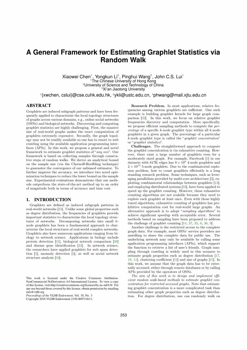
nal graph G is connected, then G(d) is also connected [35,Theorem 3.1]. Figure 1 shows an example of G(2) and G(3)
for a 4-node graph G. Let H(2) denote all 2-node inducedsubgraphs of G, then the node set of G(2) is H(2), i.e., nodepairs {(1, 2), (1, 3), (1, 4), (2, 3), (3, 4)}. Note that there is anedge between node pair (1, 2) and (2, 3) in G(2) because theyshare node 2 in G.
1 2
4 3
e1
e2
e3
e4 e5
G
1 2 2 3
3 41 4
1 3
G(2)
14
3
21
4
23
4
12
3
G(3)
Figure 1: Original graph G and its 2 and 3-nodesubgraph relationship graph G(2) and G(3).
In general, constructing G(d) is impractical due to in-tensive computation cost. However, for our random walk-based framework, there is no need to construct G(d) in ad-vance since we can generate the neighborhood subgraphs ofs 2 H(d) on the fly according to the definition of G(d).Isomorphic. Two graphs G = (V,E) and G0
= (V 0, E0)
are isomorphic if there exists a bijection ' : V ! V 0 with(v
i
, vj
) 2 E , ('(vi
),'(vj
)) 2 E0 for all vi
, vj
2 V . Sucha bijection map is called an isomorphism, and we write iso-morphic G and G0 as G ' G0.
Definition 1. Graphlets are formally defined as connected,non-isomorphic, induced subgraphs of a graph G.
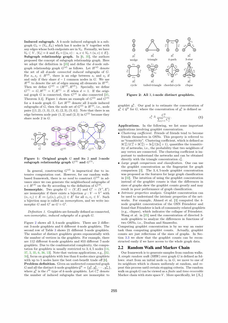
Figure 2 shows all 3, 4-node graphlets. There are 2 differ-ent 3-node graphlets and 6 different 4-node graphlets. Thesecond row of Table 3 shows 21 different 5-node graphlets.The number of distinct graphlets grows exponentially withthe number of vertices in the graphlets. For example, thereare 112 different 6-node graphlets and 853 different 7-nodegraphlets. Due to the combinatorial complexity, the compu-tation for graphlets is usually restricted to 3, 4, 5 nodes [14,37, 3, 35, 6, 36, 13]. Note that various applications, e.g., [32,34], focus on graphlets with less than 6 nodes since graphletswith up to 5 nodes have the best cost-benefit trade off [6].Problem definition. Given an undirected connected graphG and all the distinct k-node graphlets Gk
= {gk1 , gk2 , · · · , gkm},where gk
i
is the ith type of k-node graphlets. Let Ck
i
denotethe number of induced subgraphs that are isomorphic to
1
2
3
g31wedge
1
2 3
g32triangle
1
23
4
e 1
e2e3
g414-path
2
1
3 4
e1
e2
e3
g423-star
1
2 3
4
e2
e3
e 4
e1
g43cycle
3
2
1 4e1
e2 e3
e4
g44tailed-triangle
2
3
4
1e1
e2 e3
e4
e5
g45chordal-cycle
2 3
4
1
e 1 e3
e4
e2e5e6
g46clique
Figure 2: All 3, 4-node distinct graphlets.
graphlet gki
. Our goal is to estimate the concentration ofgki
2 Gk for G, where the concentration of gki
is defined as
cki
, Ck
iPm
j=1 Ck
j
. (1)
Applications. In the following, we list some importantapplications involving graphlet concentration.• Clustering coefficient. Friends of friends tend to become
friends themselves in OSNs. This property is referred toas “transitivity”. Clustering coefficient, which is defined as3C3
2/(C31 +3C3
2 ) = 3c32/(2c32 +1), quantifies the transitiv-
ity of networks, i.e., the probability that two neighbors ofany vertex are connected. The clustering coefficient is im-portant to understand the networks and can be obtaineddirectly with the triangle concentration c32.
• Large graph comparison and classification. One can usethe graphlet concentration as the fingerprint for graphcomparison [3]. The 3, 4, 5-node graphlet concentrationwas proposed as the features for large graph classificationin [32]. The intuition of using the graphlet concentrationinstead of the graphlet counts is that the differences insizes of graphs skew the graphlet counts greatly and mayresult in poor performance of graph classification.
• Intrinsic properties analysis. Graphlet concentration canbe used to understand the intrinsic properties of the net-works. For example, Ahmed et al. [3] computed the 4-node graphlet concentration of the OSN Friendster andfound that Friendster is lack of community related graphlets(e.g., cliques), which indicates the collapse of Friendster.Wang et al. in [35] used the concentration of directed 3-node graphlets to analyze the differences in functions oftwo OSNs, i.e., Douban and Sinaweibo.
Computing graphlet concentration is by no way an easiertask than computing graphlet counts. Actually, graphletcounts are just reflections of the sizes of graphs. In Sec-tion 3.3 we show that the graphlet counts can be recon-structed easily if we have access to the whole graph data.
2.2 Random Walk and Markov ChainOur framework is to generate samples from random walks.
A simple random walk (SRW) over graph G is defined as fol-lows: start from an initial node v0 in G, we move to one ofits neighbors which is chosen uniformly at random, and re-peat this process until certain stopping criteria. The randomwalk on graph G can be viewed as a finite and time-reversibleMarkov chain with state space V . More specifically, let {X
t
}
255
be the Markov chain representing the visited nodes of therandom walk on G, the transition probability matrix P ofthis Markov chain is defined as
P(i, j) =
(1di, if (i, j) 2 E,
0, otherwise.
The SRW has a unique stationary distribution ⇡⇡⇡ where ⇡(v) =dv2|E| for v 2 V [20, 26]. The stationary distribution is vitalfor correcting bias of samples generated by random walks.Strong Law of Large Numbers. Below, we review theStrong Law of Large Numbers (SLLN) for Markov chainwhich serves as the theoretical foundation for our randomwalk-based framework. For a Markov chain with finite statespace S and stationary distribution ⇡⇡⇡, we define the expec-tation of the function f : S ! R with respect to ⇡⇡⇡ as
µ = E⇡
⇡
⇡
[f ] ,X
X2S
f(X)⇡(X).
The subscript ⇡⇡⇡ indicates that the expectation is calculatedwith the assumption that X ⇠ ⇡⇡⇡. Let
µn
=
1
n
nX
s=1
f(Xs
)
denote the sample average of f(X) over a run of the Markovchain. The following theorem SLLN ensures that the samplemean converges almost surely to its expected value.
Theorem 1. [10, 17] For a finite and irreducible Markovchain with stationary distribution ⇡⇡⇡, we have
µn
! E⇡
⇡
⇡
[f ] almost surely (a.s.)
as n!1 regardless of the initial distribution of the chain.
The SLLN is the fundamental basis for most random walk-based graph sampling methods, or more formally, MarkovChain Monte Carlo (MCMC) samplers, e.g., [19, 6, 12]. TheSLLN guarantees the asymptotic unbiasedness of the esti-mators based on any finite and irreducible Markov chain.Mixing Time. The mixing time of a Markov chain is thenumber of steps it takes for a random walk to approach itsstationary distribution. We adopt the definition of mixingtime in [24, 25, 8]. The mixing time is defined as follows.
Definition 2. The mixing time ⌧(✏) (parameterized by ✏)of a Markov chain is defined as
⌧(✏) = max
Xi2Smin{t : |⇡⇡⇡ �Pt⇡⇡⇡(i)|1 < ✏},
where ⇡⇡⇡ is the stationary distribution of the Markov chain,⇡⇡⇡(i) is the initial distribution when starting from state X
i
2S, Pt is the transition matrix after t steps and | · | is thevariation distance between two distributions1.
Later on, we will use the mixing time based Chernoff-Hoeffdingbound [8] to compute the needed sample size to guaranteethat our estimate is within (1 ± ✏) of the true value withprobability at least 1� �.
1The variation distance between two distributions d1 andd2 on a countable state space S is given by |d1 � d2|1 ,12
Px2S |d1(x)� d2(x)|.
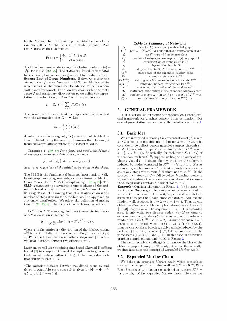
Table 1: Summary of NotationsG G = (V,E), underlying undirected graph
G(d) G(d)=(H(d),R(d)), d-node subgraph relationship graphgki
the ith type of k-node graphletsCk
i
number of subgraphs isomorphic to gki
in graph Gcki
concentration of graphlet gki
in Gdv
degree of node v in GdX
degree of state X, X is also a node in G(d)
M(l) state space of the expanded Markov chainX(l) state in state space M(l)
V (X(l)) set of graph G’s nodes contained in state X(l)
s(X(l)) subgraph induced by node set V (X(l)
)
⇡⇡⇡ stationary distribution of the random walk⇡⇡⇡e stationary distribution of the expanded Markov chain↵k
i
number of states X(l) in M(l) s.t. s ' gki
, s(X(l)) = s.
C(s) set of states X(l) in M(l) s.t. s(X(l)) = s.
3. GENERAL FRAMEWORKIn this section, we introduce our random walk-based gen-
eral framework for graphlet concentration estimation. Forease of presentation, we summary the notations in Table 1.
3.1 Basic IdeaWe are interested in finding the concentration of gk
i
, wherek � 3 (since it is not difficult to find for k = 1 or 2). Thecore idea is to collect k-node graphlet samples through l=k�d+1 consecutive steps of the random walk on G(d), whered 2 {1, . . . , k � 1}. Specifically, for each state X
i
(i � l) ofthe random walk on G(d), suppose we keep the history of pre-viously visited l � 1 states, then we consider the subgraphinduced by nodes contained in X(l)
= (Xi�l+1, . . . , Xi
) asa k-node graphlet sample. Note that we only consider con-secutive l steps which visit k distinct nodes in V . If theconsecutive l steps on G(d) fail to collect k distinct nodes inV , we just continue the random walk until we find l consec-utive steps which contain k distinct nodes in V .Example: Consider the graph in Figure 1. (a) Suppose wewant to get 3-node graphlet samples and choose a randomwalk on G. Then l = 3�1+1 = 3, i.e., we need to walk for 3steps on G to get the 3-node graphlet samples. Assume therandom walk sequence is 1! 2! 1! 4! 3. Then we canobtain two 3-node graphlet samples induced by {2, 1, 4} and{1, 4, 3} respectively. The sequence 1 ! 2 ! 1 is discardedsince it only visits two distinct nodes. (b) If we want toexplore possible graphlets g4
i
and have decided to perform arandom walk on G(2) (i.e., d = 2). Assume we make l = 3
transitions on the following states: (1, 2) ! (1, 3) ! (3, 4),then we can obtain a 4-node graphlet sample induced by thenode set {1, 2, 3, 4}, because {1, 2, 3, 4} is contained in thethree states (1, 2), (1, 3) and (3, 4). In this case, the obtainedgraphlet sample corresponds to g45 in Figure 2.
The main technical challenge is to remove the bias of theobtained graphlet samples. To analyze the bias theoretically,we first introduce the concept of expanded Markov chain.
3.2 Expanded Markov ChainWe define an expanded Markov chain which remembers
consecutive l steps of the random walk on G(d)= (H(d), R(d)
).Each l consecutive steps are considered as a state X(l)
=
(X1, · · · , Xl
) of the expanded Markov chain. Here we use
256
the superscript “l” to denote the length of the random walkblock. Each time the random walk on G(d) makes a transi-tion, the expanded Markov chain transits to the next state.Assume the expanded Markov chain is currently at stateX(l)
i
= (X1, · · · , Xl
), it means the random walker is at Xl
.If the walker jumps to X(l+1), i.e., one of the neighbors ofX
l
, then the expanded Markov chain transits to the stateX(l)
i+1 = (X2, · · · , Xl+1). Let N = H(d) denote the statespace for the random walk and M(l) denote the state spacefor the corresponding expanded Markov chain. The statespace M(l) consists of all possible consecutive l steps of therandom walk. More formally, M(l)
= {(X1, · · · , Xl
) : Xi
2N , 1 i l s.t. (X
i
, Xi+1) 2 R(d) 81 i l � 1} ✓
N ⇥ · · ·⇥N . For example, if we perform a random walk onG, any (u, v) and (v, u) where e
uv
2 E are states in M(2).Note that the expanded Markov chain describes the sameprocess as the random walk. The reason we define it here isfor the convenience of deriving unbiased estimator.
The bias caused by the non-uniform sampling probabili-ties of the graphlet samples arises from two aspects. First,the states in the expanded Markov chain have unequal sta-tionary probabilities. Second, a graphlet sample correspondsto several states in the expanded Markov chain. To derivethe unbiased estimator of the graphlet concentration, weneed to compute the stationary distribution and the num-ber of states corresponding to the same graphlet sample.Stationary distribution. Let ⇡⇡⇡ denote the stationary dis-tribution of the random walk and ⇡⇡⇡e denote the stationarydistribution of the expanded Markov chain. d
X
is number ofneighbors of state X in G(d). The following theorem statesthat ⇡⇡⇡e is unique and its value can be computed with ⇡⇡⇡.
Theorem 2. The stationary distribution ⇡⇡⇡e exists and isunique. For any X(l)
= (X1, · · · , Xl
) 2M(l), we have
⇡e
(X(l)) =
8>><
>>:
dXl
2|R(d)| if l = 1,1
2|R(d)| if l = 2,1
2|R(d)|1
dX2· · · 1
dXl�1if l > 2
(2)
The proof is in the technical report [7]. In fact, ⇡⇡⇡e can bederived directly using conditional probability formula. Forthe state X(l)
= (X1, · · · , Xl
), X1 is visited with probability⇡(X1) =
dX1
2|R(d)| during the random walk and ⇡e
(X(l)) can
be written as dX1
2|R(d)| ⇥1
dX1⇥ · · ·⇥ 1
dXl.
Example: Still using the graph in Figure 1 as an exam-ple, if we walk on G(2) and visit states X1 = (1, 2), X2 =
(1, 3), X3 = (3, 4), then the corresponding state X(3)1 in
M(3) is (X1, X2, X3). The number of edges in G(2) is 8.The degrees of X1, X2, X3 are 3, 4, 3 respectively. Then thestationary distribution of X(3)
1 is 1/16 · 1/4 = 1/64.State corresponding coefficient. Let V (X(l)
) representthe set of graph G’s nodes contained in the state X(l), ands(X(l)
) be the subgraph induced by V (X(l)). We define X(l)
as the corresponding state for the subgraph s(X(l)). A key
observation is that a subgraph may have several correspond-ing states in M(l). For example, if we perform a randomwalk on G, then a triangle induced by {u, v, w} in G has 6corresponding states (u, v, w), (u,w, v), (v, u, w), (w, v, u),(v, w, u), (w, u, v) in M(3). To describe this idea formally,we define the state corresponding coefficient ↵k
i
.
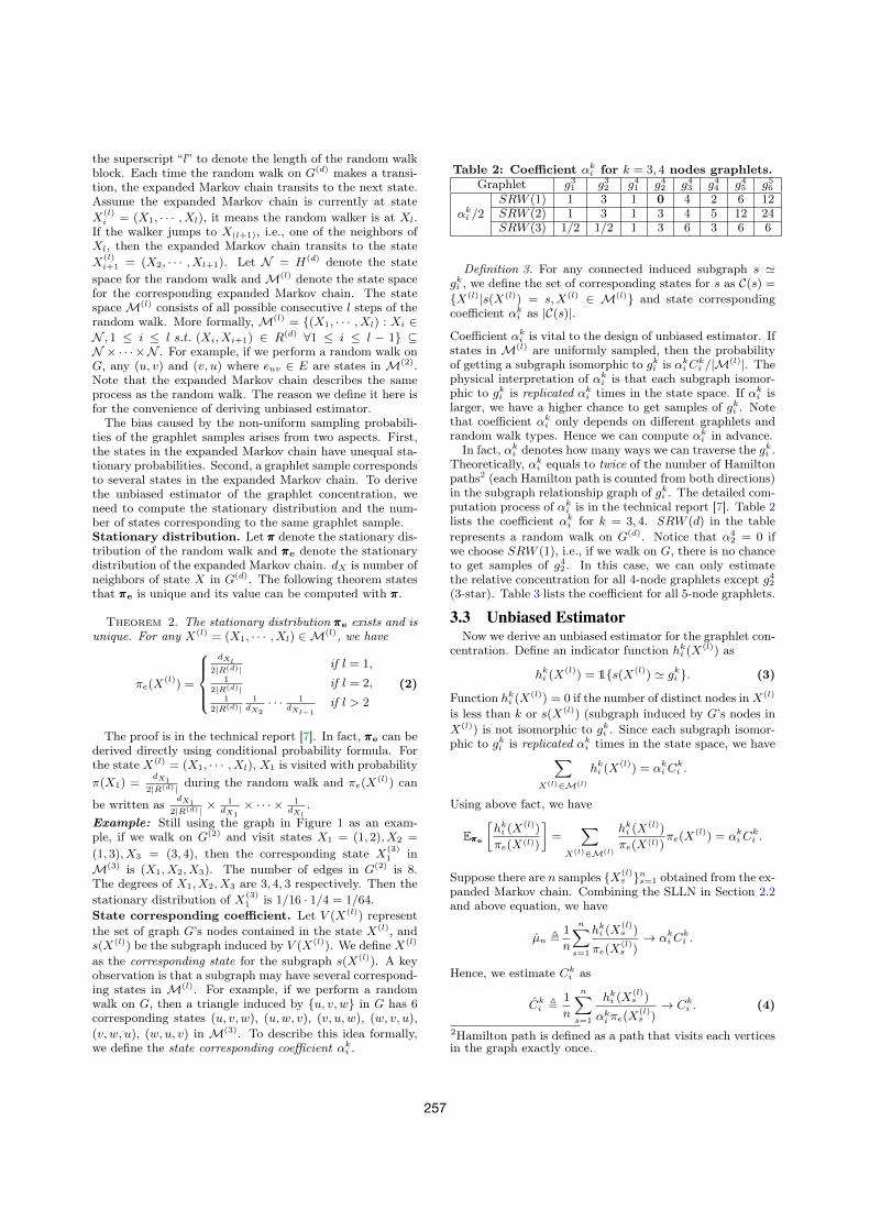
Table 2: Coefficient ↵k
i
for k = 3, 4 nodes graphlets.Graphlet g31 g32 g41 g42 g43 g44 g45 g56
↵k
i
/2SRW (1) 1 3 1 0 4 2 6 12
SRW (2) 1 3 1 3 4 5 12 24
SRW (3) 1/2 1/2 1 3 6 3 6 6
Definition 3. For any connected induced subgraph s 'gki
, we define the set of corresponding states for s as C(s) ={X(l)|s(X(l)
) = s,X(l) 2 M(l)} and state correspondingcoefficient ↵k
i
as |C(s)|.
Coefficient ↵k
i
is vital to the design of unbiased estimator. Ifstates in M(l) are uniformly sampled, then the probabilityof getting a subgraph isomorphic to gk
i
is ↵k
i
Ck
i
/|M(l)|. Thephysical interpretation of ↵k
i
is that each subgraph isomor-phic to gk
i
is replicated ↵k
i
times in the state space. If ↵k
i
islarger, we have a higher chance to get samples of gk
i
. Notethat coefficient ↵k
i
only depends on different graphlets andrandom walk types. Hence we can compute ↵k
i
in advance.In fact, ↵k
i
denotes how many ways we can traverse the gki
.Theoretically, ↵k
i
equals to twice of the number of Hamiltonpaths2 (each Hamilton path is counted from both directions)in the subgraph relationship graph of gk
i
. The detailed com-putation process of ↵k
i
is in the technical report [7]. Table 2lists the coefficient ↵k
i
for k = 3, 4. SRW (d) in the tablerepresents a random walk on G(d). Notice that ↵4
2 = 0 ifwe choose SRW (1), i.e., if we walk on G, there is no chanceto get samples of g42 . In this case, we can only estimatethe relative concentration for all 4-node graphlets except g42(3-star). Table 3 lists the coefficient for all 5-node graphlets.
3.3 Unbiased EstimatorNow we derive an unbiased estimator for the graphlet con-
centration. Define an indicator function hk
i
(X(l)) as
hk
i
(X(l)) = 1{s(X(l)
) ' gki
}. (3)
Function hk
i
(X(l)) = 0 if the number of distinct nodes in X(l)
is less than k or s(X(l)) (subgraph induced by G’s nodes in
X(l)) is not isomorphic to gki
. Since each subgraph isomor-phic to gk
i
is replicated ↵k
i
times in the state space, we haveX
X
(l)2M(l)
hk
i
(X(l)) = ↵k
i
Ck
i
.
Using above fact, we have
E⇡
⇡
⇡e
hk
i
(X(l))
⇡e
(X(l))
�=
X
X
(l)2M(l)
hk
i
(X(l))
⇡e
(X(l))
⇡e
(X(l)) = ↵k
i
Ck
i
.
Suppose there are n samples {X(l)s
}ns=1 obtained from the ex-
panded Markov chain. Combining the SLLN in Section 2.2and above equation, we have
µn
, 1
n
nX
s=1
hk
i
(X(l)s
)
⇡e
(X(l)s
)
! ↵k
i
Ck
i
.
Hence, we estimate Ck
i
as
ˆCk
i
, 1
n
nX
s=1
hk
i
(X(l)s
)
↵k
i
⇡e
(X(l)s
)
! Ck
i
. (4)
2Hamilton path is defined as a path that visits each verticesin the graph exactly once.
257
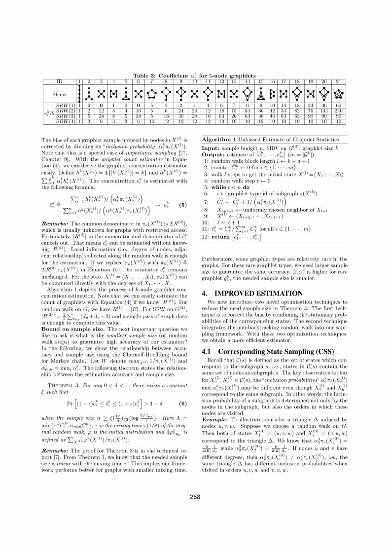
Table 3: Coefficient ↵5i
for 5-node graphletsID 1 2 3 4 5 6 7 8 9 10 11 12 13 14 15 16 17 18 19 20 21
Shape
↵5i
/2
SRW (1) 1 0 0 1 2 0 5 2 2 4 4 6 7 6 6 10 14 18 24 36 60SRW (2) 1 2 12 5 4 16 5 6 24 24 12 18 15 54 36 42 34 82 76 144 240
SRW (3) 1 5 24 8 5 24 5 16 30 24 16 63 26 63 30 43 63 63 90 90 90
SRW (4) 1 3 6 3 3 6 10 12 12 12 12 10 10 10 12 10 10 10 10 10 10
The bias of each graphlet sample induced by nodes in X(l) iscorrected by dividing its “inclusion probability” ↵k
i
⇡e
(X(l)).
Note that this is a special case of importance sampling [27,Chapter 9]. With the graphlet count estimator in Equa-tion (4), we can derive the graphlet concentration estimatoreasily. Define hk
(X(l)) = 1{|V (X(l)
)| = k} and ↵k
(X(l)) =
P|Gk|i=1 ↵k
i
hk
i
(X(l)). The concentration ck
i
is estimated withthe following formula:
cki
,P
n
s=1 hk
i
(X(l)s
)/⇣↵k
i
⇡e
(X(l)s
)
⌘
Pn
s=1 hk
(X(l)s
)/⇣↵k
(X(l)s
)⇡e
(X(l)s
)
⌘ ! cki
. (5)
Remarks: The common denominator in ⇡e
(X(l)) is 2|R(d)|,
which is usually unknown for graphs with restricted access.Fortunately, |R(d)| in the numerator and denominator of ck
i
cancels out. That means cki
can be estimated without know-ing |R(d)|. Local information (i.e., degree of nodes, adja-cent relationship) collected along the random walk is enoughfor the estimation. If we replace ⇡
e
(X(l)) with ⇡
e
(X(l)) ,
2|R(d)|⇡e
(X(l)) in Equation (5), the estimator ck
i
remainsunchanged. For the state X(l)
= (X1, · · · , Xl
), ⇡e
(X(l)) can
be computed directly with the degrees of X1, · · · , Xl
.Algorithm 1 depicts the process of k-node graphlet con-
centration estimation. Note that we can easily estimate thecount of graphlets with Equation (4) if we know |R(d)|. Forrandom walk on G, we have R(1)
= |E|. For SRW on G(2),|R(2)| = 1
2
Peuv
(du
+dv
�2) and a single pass of graph datais enough to compute this value.Bound on sample size. The next important question welike to ask is what is the smallest sample size (or randomwalk steps) to guarantee high accuracy of our estimator?In the following, we show the relationship between accu-racy and sample size using the Chernoff-Hoeffding boundfor Markov chain. Let W denote max
X
(l) 1/⇡e
(X(l)) and
↵min = min
i
↵k
i
. The following theorem states the relation-ship between the estimation accuracy and sample size.
Theorem 3. For any 0 < � < 1, there exists a constant⇠ such that
Pr
h(1� ✏)ck
i
cki
(1 + ✏)cki
i> 1� � (6)
when the sample size n � ⇠(W⇤ )
⌧
✏
2 (logk'k⇡⇡⇡e
�
). Here ⇤ =
min{↵k
i
Ck
i
,↵minCk}, ⌧ is the mixing time ⌧(1/8) of the orig-
inal random walk, ' is the initial distribution and k'k⇡
⇡
⇡eis
defined asP
X
(l) '2(X(l)
)/⇡e
(X(l)).
Remarks: The proof for Theorem 3 is in the technical re-port [7]. From Theorem 3, we know that the needed samplesize is linear with the mixing time ⌧ . This implies our frame-work performs better for graphs with smaller mixing time.
Algorithm 1 Unbiased Estimate of Graphlet StatisticsInput: sample budget n, SRW on G(d), graphlet size kOutput: estimate of
⇥ck1 , · · · , ckm
⇤(m = |Gk|)
1: random walk block length l k � d+ 1
2: counter ˆCk
i
0 for i 2 {1, · · · ,m}3: walk l steps to get the initial state X(l)
=(X1,· · · ,Xl
)
4: random walk step t 0
5: while t < n do6: i graphlet type id of subgraph s(X(l)
)
7: ˆCk
i
ˆCk
i
+ 1/⇣↵k
i
⇡e
(X(l))
⌘
8: Xl+t+1 uniformly chosen neighbor of X
l+t
9: X(l) (Xt+2, · · · , Xl+t+1)
10: t t+ 1
11: cki
=
ˆCk
i
/P
m
j=1ˆCk
j
for all i 2 {1, · · · ,m}12: return
⇥ck1 , · · · , ckm
⇤
Furthermore, some graphlet types are relatively rare in thegraphs. For these rare graphlet types, we need larger samplesize to guarantee the same accuracy. If ↵k
i
is higher for raregraphlet gk
i
, the needed sample size is smaller.
4. IMPROVED ESTIMATIONWe now introduce two novel optimization techniques to
reduce the need sample size in Theorem 3. The first tech-nique is to correct the bias by combining the stationary prob-abilities of the corresponding states. The second techniqueintegrates the non-backtracking random walk into our sam-pling framework. With these two optimization techniques,we obtain a more efficient estimator.
4.1 Corresponding State Sampling (CSS)Recall that C(s) is defined as the set of states which cor-
respond to the subgraph s, i.e., states in C(s) contain thesame set of nodes as subgraph s. The key observation is thatfor X(l)
a
, X(l)b
2 C(s), the “inclusion probabilities” ↵k
i
⇡e
(X(l)a
)
and ↵k
i
⇡e
(X(l)b
) may be different even though X(l)a
and X(l)b
correspond to the same subgraph. In other words, the inclu-sion probability of a subgraph is determined not only by thenodes in the subgraph, but also the orders in which thesenodes are visited.Example: To illustrate, consider a triangle � induced bynodes u, v, w. Suppose we choose a random walk on G.Then both of states X(3)
1 = (u, v, w) and X(3)2 = (v, u, w)
correspond to the triangle �. We know that ↵32⇡e
(X(3)1 ) =
62|E|
1dv
while ↵32⇡e
(X(3)2 ) =
62|E|
1du
. If nodes u and v havedifferent degrees, then ↵3
2⇡e
(X(3)1 ) 6= ↵3
2⇡e
(X(3)2 ), i.e., the
same triangle � has different inclusion probabilities whenvisited in orders u, v, w and v, u, w.
258
Based on this observation3, we define “sampling probabil-ity” p(X(l)
) for the subgraph induced by nodes in X(l). Thevalue of p(X(l)
) only depends degrees of nodes in X(l).
Definition 4. For a state X(l) and a subgraph s = s(X(l)),
we define the sampling probability for s as
p(X(l)) ,
X
X
(l)j 2C(s)
⇡e
(X(l)j
).
In the following, we prove that if we substitute ↵k
i
⇡e
(X(l))
with p(X(l)) in Equation (4), we still obtain an unbiased
estimator of Ck
i
.
Lemma 4. For a specific subgraph s ' gki
, we have
E⇡
⇡
⇡e [1
↵k
i
⇡e
X(l)1{V (X(l)
) = V (s)}] =
E⇡
⇡
⇡e [1
p(X(l))
1{V (X(l)) = V (s)}]
Lemma 4 can be proved directly using the definition. It istrivial to verify that the function hk
i
(X(l)) in Equation (3)
is the linear combination of function 1{V (X(l)) = V (s)}.
Using the linearity of expectation and the result in Lemma 4,we have
E⇡
⇡
⇡e
hk
i
(X(l))
p(X(l))
�= E
⇡
⇡
⇡e
hk
i
(X(l))
↵k
i
⇡e
(X(l))
�.
Hence, we can rewrite the estimator in Equation (4) as
1
n
nX
s=1
hk
i
(X(l)s
)
p(X(l)s
)
! Ck
i
a.s. (7)
Similarly, we estimate graphlet concentration asP
n
s=1 hk
i
(X(l)s
)/p(X(l)s
)
Pn
s=1 hk
(X(l)s
)/p(X(l)s
)
! cki
a.s. (8)
Remarks: The pseudo code of computing p(X(l)) is pre-
sented in the technical report [7]. The estimator in Equa-tion (7) corrects the bias of graphlet samples using the sam-pling probability p(X(l)
) instead of ↵k
i
⇡e
(X(l)). It indicates
that the probability that a subgraph s is generated by therandom walk actually equals to
PX
(l)j 2C(s) ⇡e
(X(l)j
).
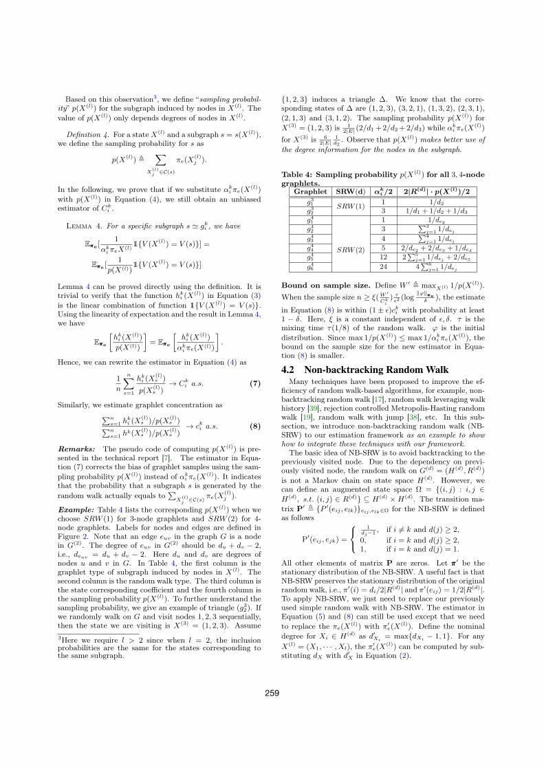
Example: Table 4 lists the corresponding p(X(l)) when we
choose SRW (1) for 3-node graphlets and SRW (2) for 4-node graphlets. Labels for nodes and edges are defined inFigure 2. Note that an edge e
uv
in the graph G is a nodein G(2). The degree of e
uv
in G(2) should be du
+ dv
� 2,i.e., d
euv = du
+ dv
� 2. Here du
and dv
are degrees ofnodes u and v in G. In Table 4, the first column is thegraphlet type of subgraph induced by nodes in X(l). Thesecond column is the random walk type. The third column isthe state corresponding coefficient and the fourth column isthe sampling probability p(X(l)
). To further understand thesampling probability, we give an example of triangle (g32). Ifwe randomly walk on G and visit nodes 1, 2, 3 sequentially,then the state we are visiting is X(3)
= (1, 2, 3). Assume3Here we require l > 2 since when l = 2, the inclusionprobabilities are the same for the states corresponding tothe same subgraph.
{1, 2, 3} induces a triangle �. We know that the corre-sponding states of � are (1, 2, 3), (3, 2, 1), (1, 3, 2), (2, 3, 1),(2, 1, 3) and (3, 1, 2). The sampling probability p(X(l)
) forX(3)
= (1, 2, 3) is 12|E| (2/d1+2/d2+2/d3) while ↵k
i
⇡e
(X(l))
for X(3) is 62|E|
1d2
. Observe that p(X(l)) makes better use of
the degree information for the nodes in the subgraph.
Table 4: Sampling probability p(X(l)) for all 3, 4-node
graphlets.Graphlet SRW(d) ↵k
i /2 2|R(d)| · p(X(l))/2
g31 SRW (1)
1 1/d2g32 3 1/d1 + 1/d2 + 1/d3g41 1 1/d
e2
g42
SRW (2)
3P3
j=1 1/dejg43 4
P4j=1 1/dej
g44 5 2/de2 + 2/d
e3 + 1/de4
g45 12 2
P5j=1 1/dej + 2/d
e5
g46 24 4
P6j=1 1/dej
Bound on sample size. Define W 0 , max
X
(l) 1/p(X(l)).
When the sample size n � ⇠(W0
C
ki)
⌧
✏
2 (logk'k⇡⇡⇡e
�
), the estimate
in Equation (8) is within (1± ✏)cki
with probability at least1 � �. Here, ⇠ is a constant independent of ✏, �. ⌧ is themixing time ⌧(1/8) of the random walk. ' is the initialdistribution. Since max 1/p(X(l)
) max 1/↵k
i
⇡e
(X(l)), the
bound on the sample size for the new estimator in Equa-tion (8) is smaller.
4.2 Non-backtracking Random WalkMany techniques have been proposed to improve the ef-
ficiency of random walk-based algorithms, for example, non-backtracking random walk [17], random walk leveraging walkhistory [39], rejection controlled Metropolis-Hasting randomwalk [19], random walk with jump [38], etc. In this sub-section, we introduce non-backtracking random walk (NB-SRW) to our estimation framework as an example to showhow to integrate these techniques with our framework.
The basic idea of NB-SRW is to avoid backtracking to thepreviously visited node. Due to the dependency on previ-ously visited node, the random walk on G(d)
= (H(d), R(d))
is not a Markov chain on state space H(d). However, wecan define an augmented state space ⌦ = {(i, j) : i, j 2H(d), s.t. (i, j) 2 R(d)} ✓ H(d) ⇥H(d). The transition ma-trix P0 , {P 0
(eij
, elk
)}eij ,elk2⌦ for the NB-SRW is defined
as follows
P
0(e
ij
, ejk
) =
8<
:
1dj�1 , if i 6= k and d(j) � 2,
0, if i = k and d(j) � 2,1, if i = k and d(j) = 1.
All other elements of matrix P are zeros. Let ⇡⇡⇡0 be thestationary distribution of the NB-SRW. A useful fact is thatNB-SRW preserves the stationary distribution of the originalrandom walk, i.e., ⇡0
(i) = di
/2|R(d)| and ⇡0(e
ij
) = 1/2|R(d)|.To apply NB-SRW, we just need to replace our previouslyused simple random walk with NB-SRW. The estimator inEquation (5) and (8) can still be used except that we needto replace the ⇡
e
(X(l)) with ⇡0
e
(X(l)). Define the nominal
degree for Xi
2 H(d) as d0Xi
= max{dXi � 1, 1}. For any
X(l)= (X1, · · · , Xl
), the ⇡0e
(X(l)) can be computed by sub-
stituting dX
with d0X
in Equation (2).
259
Applying NB-SRW helps us eliminate some “invalid” statesfrom the state space. For example, if we want to estimate3-node graphlet concentration using SRW (1), we need towalk for 3 steps on G to collect a sample. It is possible forus to get only 2 distinct nodes from 3 steps. We call suchsamples as invalid samples. The invalid samples do not con-tribute to the estimation. If we apply NB-SRW here, it isless likely to get such invalid samples. Hence NB-SRW helpsto improve the estimation efficiency of our framework.
5. IMPLEMENTATION DETAILSWe explain how to obtain neighbors of currently visited
state (subgraph) s 2 H(d) on the fly. Obtaining a uniformlychosen neighbor of a node in G or G(2) takes O(1) time.We give details about the random walk on G(2). The set ofneighbors of e
uv
is N(euv
) = {euw
: w 2 N(u)\v} [ {evz
:
z 2 N(v)\u}. Recall that N(v) denotes the set of neighborsof v 2 V . To ensure each neighbor of e
uv
is chosen uniformly,we first select one of u and v with probability d
u
/(du
+ dv
)
and dv
/(du
+dv
) respectively. Suppose we have chosen nodeu, we then randomly select a node w 2 N(u). If w 6= v, e
uw
is proposed as the next step after euv
. Otherwise, we restartthe process until we obtain a neighbor of e
uv
. Based onabove discussion, we know that getting a uniformly sampledneighbor of a state in G(2) can be done in constant time.
To obtain a randomly chosen neighbor of s in G(d), we canreplace one node v
i
in V (s) with a node vj
2 [v2V (s)\viN(v)
and ensure the connectivity of this new subgraph inducedby node set {v
j
} [ V (s)\vi
. Here V (s) is the node set ofthe subgraph s. However, to ensure the neighbors of s areuniformly sampled, we need to generate all neighbors of swhen d > 2, which requires d merge operations over d � 1
adjacent lists of nodes in the currently visited subgraph.Hence, the time complexity of selecting a random neighborfor a state in G(d) is simply O(d2 |E|
|V | ) when d > 2.According to Algorithm 1, we also need to identify the
graphlet type of the obtained samples at each step. Werefer interested readers to the implementation details andtime complexity analysis in the technical report [7].
Note that our framework does not need any preprocessingof the graph data. The time complexity of our framework isO(n) when d 2 and O(nd2 |E|
|V | ) when d > 2 for the k-nodegraphlets. Here n is the random walk steps.
6. EXPERIMENTAL EVALUATIONWe evaluate the performance of our framework on 3, 4, 5-
node graphlets. The algorithms are implemented in C++ andwe run experiments on a Linux machine with Intel 3.70GHzCPU. We aim to answer the following questions.Q1: How accurate is our framework? Do the optimization
techniques really improve the accuracy?Q2: How does the random walk on G(d) affect the perfor-
mance? What is the best parameter d for 3, 4, 5-nodegraphlets?
Q3: Does our framework provide more accurate estimationthan the state-of-the-art methods?
6.1 Experiment SetupWe use publicly available real-world networks to evaluate
our framework. We focus on undirected graphs by removingthe directions of edges if the graphs are directed. We onlyretain the largest connected component (LCC) of the graphs
and discard the rest nodes and edges. The detailed infor-mation about the LCC of the graphs is reported in Table 5.
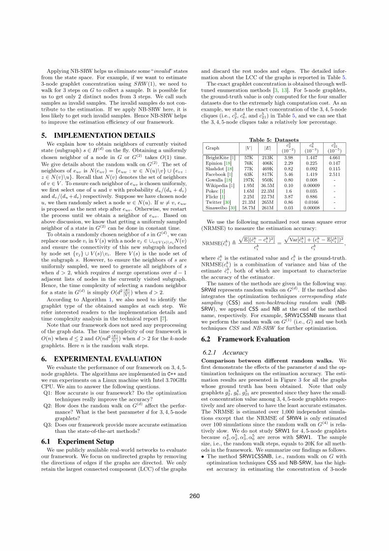
The exact graphlet concentration is obtained through well-tuned enumeration methods [3, 13]. For 5-node graphlets,the ground-truth value is only computed for the four smallerdatasets due to the extremely high computation cost. As anexample, we state the exact concentration of the 3, 4, 5-nodecliques (i.e., c32, c46, and c521) in Table 5, and we can see thatthe 3, 4, 5-node cliques take a relatively low percentage.
Table 5: DatasetsGraph |V | |E| c32
(10�2)c46
(10�3)c521
(10�5)BrightKite [1] 57K 213K 3.98 1.447 4.661Epinion [18] 76K 406K 2.29 0.225 0.147Slashdot [18] 77K 469K 0.82 0.092 0.115Facebook [1] 63K 817K 5.46 1.419 2.511Gowalla [18] 197K 950K 0.80 0.008 -Wikipedia [1] 1.9M 36.5M 0.10 0.00009 -Pokec [1] 1.6M 22.3M 1.6 0.035 -Flickr [1] 2.2M 22.7M 3.87 0.886 -Twitter [30] 21.3M 265M 0.86 0.0166 -Sinaweibo [30] 58.7M 261M 0.03 0.00008 -
We use the following normalized root mean square error(NRMSE) to measure the estimation accuracy:
NRMSE(cki
) ,p
E[(cki
� cki
)
2]
cki
=
pVar[ck
i
] + (cki
� E[cki
])
2
cki
,
where cki
is the estimated value and cki
is the ground-truth.NRMSE(ck
i
) is a combination of variance and bias of theestimate ck
i
, both of which are important to characterizethe accuracy of the estimator.
The names of the methods are given in the following way.SRWd represents random walks on G(d). If the method alsointegrates the optimization techniques corresponding statesampling (CSS) and non-backtracking random walk (NB-
SRW), we append CSS and NB at the end of the methodname, respectively. For example, SRW1CSSNB means thatwe perform the random walk on G(1) (i.e., G) and use bothtechniques CSS and NB-SRW for further optimization.
6.2 Framework Evaluation
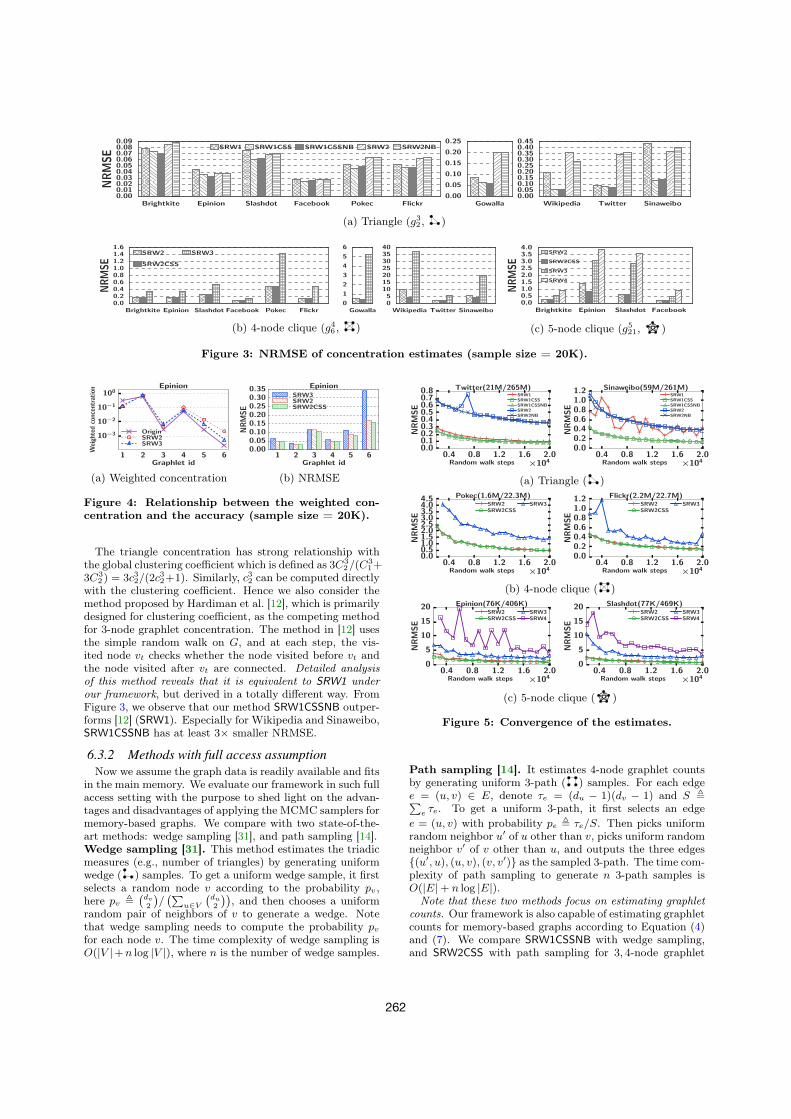
6.2.1 Accuracy
Comparison between different random walks. Wefirst demonstrate the effects of the parameter d and the op-timization techniques on the estimation accuracy. The esti-mation results are presented in Figure 3 for all the graphswhose ground truth has been obtained. Note that onlygraphlets g32 , g46 , g521 are presented since they have the small-est concentration value among 3, 4, 5-node graphlets respec-tively and are observed to have the least accurate estimates.The NRMSE is estimated over 1,000 independent simula-tions except that the NRMSE of SRW4 is only estimatedover 100 simulations since the random walk on G(4) is rela-tively slow. We do not study SRW1 for 4, 5-node graphletsbecause ↵4
2,↵52,↵
53,↵
56 are zeros with SRW1. The sample
size, i.e., the random walk steps, equals to 20K for all meth-ods in the framework. We summarize our findings as follows.• The method SRW1CSSNB, i.e., random walk on G with
optimization techniques CSS and NB-SRW, has the high-est accuracy in estimating the concentration of 3-node
260
graphlets. The method SRW2CSS has the best perfor-mance in estimating 4, 5-node graphlet concentration.
• The best methods in our framework provide accurate es-timates. The NRMSE of SRW1CSSNB for graphlet g32 isin the range 0.025 ⇠ 0.13. The NRMSE of SRW2CSS
for graphlets g46 , g521 is in the range 0.08 ⇠ 4.3, and 0.20 ⇠0.86 respectively. Note that we only use 20K random walksteps. The sample size is small compared with the graphsize. E.g., we only exploit 0.03% nodes of Sinaweibo.
• For the same graphlets, the random walk on G(d) withsmaller d outputs better estimates. E.g., SRW1 outputsestimates of c32 which has 3.8⇥ smaller NRMSE than thatof SRW2 for Twitter; SRW2 produces estimates of c46 with10⇥ smaller NRMSE than SRW3 for Gowalla. In con-clusion, we should choose d = {1, 2, 2} for 3, 4, 5-nodegraphlets respectively.
• The optimization technique CSS improves the accuracy ofestimates a lot while the performance gain of NB-SRW isnegligible. For example, SRW1CSS reduces the NRMSEof SRW1 more than 3 times for Wikipedia and Sinaweibowhen estimating the triangle (g32) concentration.
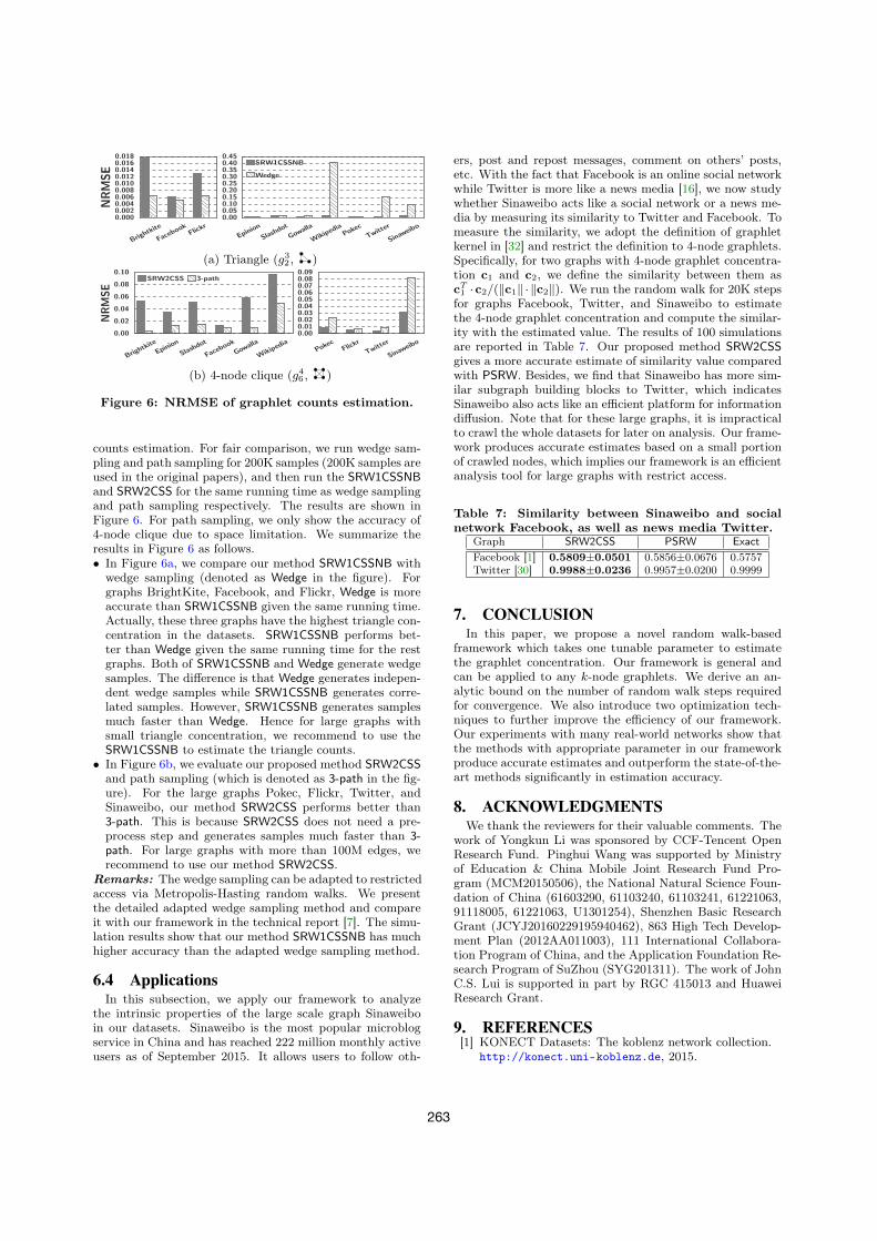
Weighted concentration and accuracy. We now in-troduce the concept of weighted concentration to explainhow the parameter d affects the performance. From Equa-tion (4), we know that 1
n
Pn
s=1h
ki (X
(l)s )
⇡e(X(l)s )! ↵k
i
Ck
i
. To furtherunderstand the performance of our framework, we define theweighted concentration for graphlet gk
i
as ↵k
i
Ck
i
/(P
m
j=1 ↵k
j
Ck
j
).As an example, we plot the weighted concentration of 4-nodegraphlets for Epinion in Figure 4a. From Figure 4, we knowthe parameter d and the concentration value affect the per-formance of our framework in the following way.• Effect of the parameter d. Compared with the origi-
nal concentration, the weighted version lifts the percent-age of relatively rare graphlets, i.e., g43 ( ), g45 ( ),and g46 ( ). For the graphs Epinion, the weighted con-centration of SRW2 is much larger than that of SRW3
for graphlets g45 , g46 , while for graphlet g43 , the weighted
concentration of SRW3 is slightly higher than that ofSRW2. For example, the weighted concentration for g46with SRW2 is about 8⇥ higher than the original one whileSRW3 only increases the concentration 2⇥ higher. Inother words, SRW2 increases the probability of getting asample of g46 about 8⇥ higher compared with uniform sam-pling of graphlets, while SRW3 only increases the prob-ability about 2⇥ higher. Consequently, the NRMSE ofSRW2 in estimating c46 is 2⇥ smaller than that of SRW3.From Theorem 3 we know that more samples are needed toachieve specific accuracy for graphlets with smaller ↵k
i
Ck
i
.Hence the error of the estimation for rare graphlets is themajor error source. If we are able to assign rare graphletshigher weighted concentration, the overall performance isless likely to degenerate. Based on above discussion, weconclude that random walks on G(d) with smaller d havebetter overall performance since they have a higher chanceof getting the relatively rare graphlets.
• Effect of the concentration value. From Figure 4b wecan see that SRW2 and SRW2CSS perform better thanSRW3 for all the 4-node graphlets except g43 (becausethe weighted concentration of g43 computed with SRW3 ishigher than that of SRW2). Besides, the smaller the con-centration value, the higher the estimation error, which isconsistent with our analysis in Theorem 3.
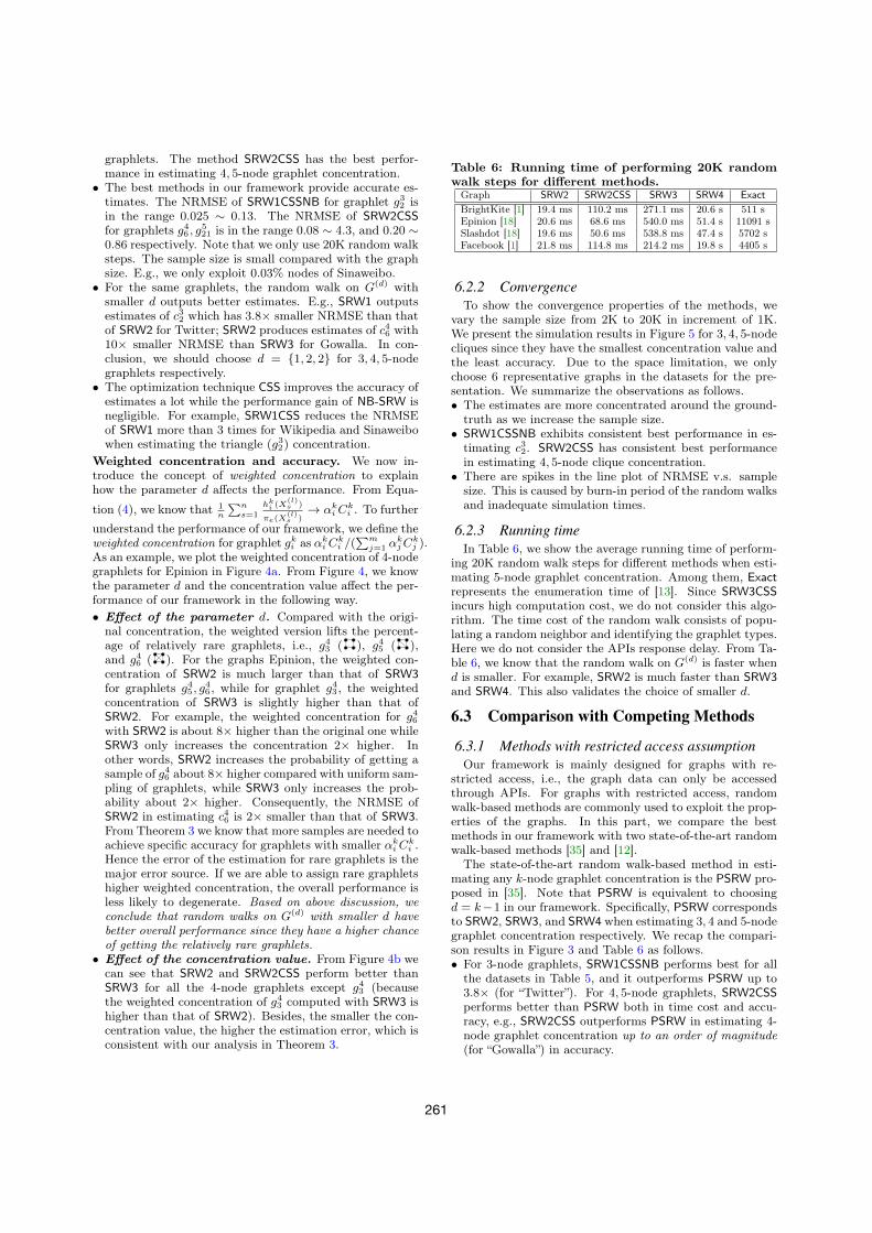
Table 6: Running time of performing 20K randomwalk steps for different methods.
Graph SRW2 SRW2CSS SRW3 SRW4 Exact
BrightKite [1] 19.4 ms 110.2 ms 271.1 ms 20.6 s 511 sEpinion [18] 20.6 ms 68.6 ms 540.0 ms 51.4 s 11091 sSlashdot [18] 19.6 ms 50.6 ms 538.8 ms 47.4 s 5702 sFacebook [1] 21.8 ms 114.8 ms 214.2 ms 19.8 s 4405 s
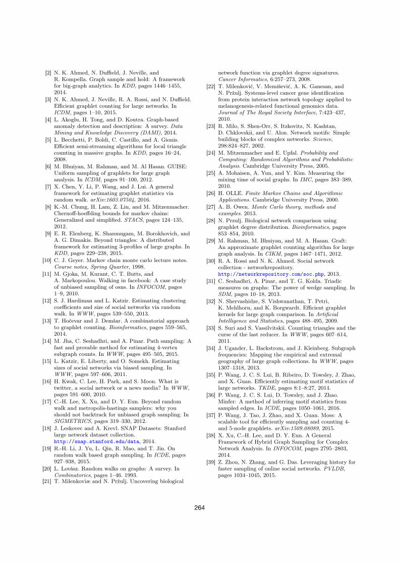
6.2.2 Convergence
To show the convergence properties of the methods, wevary the sample size from 2K to 20K in increment of 1K.We present the simulation results in Figure 5 for 3, 4, 5-nodecliques since they have the smallest concentration value andthe least accuracy. Due to the space limitation, we onlychoose 6 representative graphs in the datasets for the pre-sentation. We summarize the observations as follows.• The estimates are more concentrated around the ground-
truth as we increase the sample size.• SRW1CSSNB exhibits consistent best performance in es-
timating c32. SRW2CSS has consistent best performancein estimating 4, 5-node clique concentration.
• There are spikes in the line plot of NRMSE v.s. samplesize. This is caused by burn-in period of the random walksand inadequate simulation times.
6.2.3 Running time
In Table 6, we show the average running time of perform-ing 20K random walk steps for different methods when esti-mating 5-node graphlet concentration. Among them, Exact
represents the enumeration time of [13]. Since SRW3CSS
incurs high computation cost, we do not consider this algo-rithm. The time cost of the random walk consists of popu-lating a random neighbor and identifying the graphlet types.Here we do not consider the APIs response delay. From Ta-ble 6, we know that the random walk on G(d) is faster whend is smaller. For example, SRW2 is much faster than SRW3
and SRW4. This also validates the choice of smaller d.
6.3 Comparison with Competing Methods
6.3.1 Methods with restricted access assumption
Our framework is mainly designed for graphs with re-stricted access, i.e., the graph data can only be accessedthrough APIs. For graphs with restricted access, randomwalk-based methods are commonly used to exploit the prop-erties of the graphs. In this part, we compare the bestmethods in our framework with two state-of-the-art randomwalk-based methods [35] and [12].
The state-of-the-art random walk-based method in esti-mating any k-node graphlet concentration is the PSRW pro-posed in [35]. Note that PSRW is equivalent to choosingd = k�1 in our framework. Specifically, PSRW correspondsto SRW2, SRW3, and SRW4 when estimating 3, 4 and 5-nodegraphlet concentration respectively. We recap the compari-son results in Figure 3 and Table 6 as follows.• For 3-node graphlets, SRW1CSSNB performs best for all
the datasets in Table 5, and it outperforms PSRW up to3.8⇥ (for “Twitter”). For 4, 5-node graphlets, SRW2CSS
performs better than PSRW both in time cost and accu-racy, e.g., SRW2CSS outperforms PSRW in estimating 4-node graphlet concentration up to an order of magnitude(for “Gowalla”) in accuracy.
261
Brightkite Epinion Slashdot Facebook Pokec Flickr0.000.010.020.030.040.050.060.070.080.09
NRM
SE
SRW1 SRW1CSS SRW1CSSNB SRW2 SRW2NB
Gowalla0.00
0.05
0.10
0.15
0.20
0.25
Wikipedia Twitter Sinaweibo0.000.050.100.150.200.250.300.350.400.45
(a) Triangle (g32 , )
Brightkite Epinion Slashdot Facebook Pokec Flickr0.00.20.40.60.81.01.21.41.6
NRM
SE
SRW2
SRW2CSS
SRW3
Gowalla0
1
2
3
4
5
6
Wikipedia Twitter Sinaweibo05
10152025303540
(b) 4-node clique (g46 , )
Brightkite Epinion Slashdot Facebook0.00.51.01.52.02.53.03.54.0
NRM
SE
SRW2
SRW2CSS
SRW3
SRW4
(c) 5-node clique (g521, )
Figure 3: NRMSE of concentration estimates (sample size = 20K).
1 2 3 4 5 6Graphlet id
10�3
10�2
10�1
100
Wei
ghte
dco
ncen
trat
ion Epinion
OriginSRW2SRW3
(a) Weighted concentration
1 2 3 4 5 6Graphlet id
0.000.050.100.150.200.250.300.35
NRM
SE
EpinionSRW3SRW2SRW2CSS
(b) NRMSE
Figure 4: Relationship between the weighted con-centration and the accuracy (sample size = 20K).
The triangle concentration has strong relationship withthe global clustering coefficient which is defined as 3C3
2/(C31+
3C32 ) = 3c32/(2c
32+1). Similarly, c32 can be computed directly
with the clustering coefficient. Hence we also consider themethod proposed by Hardiman et al. [12], which is primarilydesigned for clustering coefficient, as the competing methodfor 3-node graphlet concentration. The method in [12] usesthe simple random walk on G, and at each step, the vis-ited node v
t
checks whether the node visited before vt
andthe node visited after v
t
are connected. Detailed analysisof this method reveals that it is equivalent to SRW1 underour framework, but derived in a totally different way. FromFigure 3, we observe that our method SRW1CSSNB outper-forms [12] (SRW1). Especially for Wikipedia and Sinaweibo,SRW1CSSNB has at least 3⇥ smaller NRMSE.
6.3.2 Methods with full access assumption
Now we assume the graph data is readily available and fitsin the main memory. We evaluate our framework in such fullaccess setting with the purpose to shed light on the advan-tages and disadvantages of applying the MCMC samplers formemory-based graphs. We compare with two state-of-the-art methods: wedge sampling [31], and path sampling [14].Wedge sampling [31]. This method estimates the triadicmeasures (e.g., number of triangles) by generating uniformwedge ( ) samples. To get a uniform wedge sample, it firstselects a random node v according to the probability p
v
,here p
v
,�dv2
�/�P
u2V
�du2
��, and then chooses a uniform
random pair of neighbors of v to generate a wedge. Notethat wedge sampling needs to compute the probability p
v
for each node v. The time complexity of wedge sampling isO(|V |+n log |V |), where n is the number of wedge samples.
0.4 0.8 1.2 1.6 2.0Random walk steps �104
0.00.10.20.30.40.50.60.70.8
NRM
SE
Twitter(21M/265M)SRW1SRW1CSSSRW1CSSNBSRW2SRW2NB
0.4 0.8 1.2 1.6 2.0Random walk steps �104
0.00.20.40.60.81.01.2
NRM
SE
Sinaweibo(59M/261M)SRW1SRW1CSSSRW1CSSNBSRW2SRW2NB
(a) Triangle ( )
0.4 0.8 1.2 1.6 2.0Random walk steps �104
0.00.51.01.52.02.53.03.54.04.5
NRM
SE
Pokec(1.6M/22.3M)SRW2SRW2CSS
SRW3
0.4 0.8 1.2 1.6 2.0Random walk steps �104
0.00.20.40.60.81.01.2
NRM
SE
Flickr(2.2M/22.7M)SRW2SRW2CSS
SRW3
(b) 4-node clique ( )
0.4 0.8 1.2 1.6 2.0Random walk steps �104
0
5
10
15
20
NRM
SE
Epinion(76K/406K)SRW2SRW2CSS
SRW3SRW4
0.4 0.8 1.2 1.6 2.0Random walk steps �104
0
5
10
15
20
NRM
SE
Slashdot(77K/469K)SRW2SRW2CSS
SRW3SRW4
(c) 5-node clique ( )
Figure 5: Convergence of the estimates.
Path sampling [14]. It estimates 4-node graphlet countsby generating uniform 3-path ( ) samples. For each edgee = (u, v) 2 E, denote ⌧
e
= (du
� 1)(dv
� 1) and S ,Pe
⌧e
. To get a uniform 3-path, it first selects an edgee = (u, v) with probability p
e
, ⌧e
/S. Then picks uniformrandom neighbor u0 of u other than v, picks uniform randomneighbor v0 of v other than u, and outputs the three edges{(u0, u), (u, v), (v, v0)} as the sampled 3-path. The time com-plexity of path sampling to generate n 3-path samples isO(|E|+ n log |E|).
Note that these two methods focus on estimating graphletcounts. Our framework is also capable of estimating graphletcounts for memory-based graphs according to Equation (4)and (7). We compare SRW1CSSNB with wedge sampling,and SRW2CSS with path sampling for 3, 4-node graphlet
262
Brightk
ite
Facebo
okFlic
kr0.0000.0020.0040.0060.0080.0100.0120.0140.0160.018
NRM
SE
Epinion
Slashd
ot
Gowalla
Wikipedi
aPoke
c
Sinaw
eibo
0.000.050.100.150.200.250.300.350.400.45
SRW1CSSNB
Wedge
(a) Triangle (g32 , )
Brightk
ite
Epinion
Slashd
ot
Facebo
ok
Gowalla
Wikipedi
a0.00
0.02
0.04
0.06
0.08
0.10
NRM
SE
SRW2CSS 3-path
Pokec
Flickr
Sinaw
eibo
0.000.010.020.030.040.050.060.070.080.09
(b) 4-node clique (g46 , )
Figure 6: NRMSE of graphlet counts estimation.
counts estimation. For fair comparison, we run wedge sam-pling and path sampling for 200K samples (200K samples areused in the original papers), and then run the SRW1CSSNB
and SRW2CSS for the same running time as wedge samplingand path sampling respectively. The results are shown inFigure 6. For path sampling, we only show the accuracy of4-node clique due to space limitation. We summarize theresults in Figure 6 as follows.• In Figure 6a, we compare our method SRW1CSSNB with
wedge sampling (denoted as Wedge in the figure). Forgraphs BrightKite, Facebook, and Flickr, Wedge is moreaccurate than SRW1CSSNB given the same running time.Actually, these three graphs have the highest triangle con-centration in the datasets. SRW1CSSNB performs bet-ter than Wedge given the same running time for the restgraphs. Both of SRW1CSSNB and Wedge generate wedgesamples. The difference is that Wedge generates indepen-dent wedge samples while SRW1CSSNB generates corre-lated samples. However, SRW1CSSNB generates samplesmuch faster than Wedge. Hence for large graphs withsmall triangle concentration, we recommend to use theSRW1CSSNB to estimate the triangle counts.
• In Figure 6b, we evaluate our proposed method SRW2CSS
and path sampling (which is denoted as 3-path in the fig-ure). For the large graphs Pokec, Flickr, Twitter, andSinaweibo, our method SRW2CSS performs better than3-path. This is because SRW2CSS does not need a pre-process step and generates samples much faster than 3-
path. For large graphs with more than 100M edges, werecommend to use our method SRW2CSS.
Remarks: The wedge sampling can be adapted to restrictedaccess via Metropolis-Hasting random walks. We presentthe detailed adapted wedge sampling method and compareit with our framework in the technical report [7]. The simu-lation results show that our method SRW1CSSNB has muchhigher accuracy than the adapted wedge sampling method.
6.4 ApplicationsIn this subsection, we apply our framework to analyze
the intrinsic properties of the large scale graph Sinaweiboin our datasets. Sinaweibo is the most popular microblogservice in China and has reached 222 million monthly activeusers as of September 2015. It allows users to follow oth-
ers, post and repost messages, comment on others’ posts,etc. With the fact that Facebook is an online social networkwhile Twitter is more like a news media [16], we now studywhether Sinaweibo acts like a social network or a news me-dia by measuring its similarity to Twitter and Facebook. Tomeasure the similarity, we adopt the definition of graphletkernel in [32] and restrict the definition to 4-node graphlets.Specifically, for two graphs with 4-node graphlet concentra-tion c1 and c2, we define the similarity between them ascT1 ·c2/(kc1k ·kc2k). We run the random walk for 20K stepsfor graphs Facebook, Twitter, and Sinaweibo to estimatethe 4-node graphlet concentration and compute the similar-ity with the estimated value. The results of 100 simulationsare reported in Table 7. Our proposed method SRW2CSS
gives a more accurate estimate of similarity value comparedwith PSRW. Besides, we find that Sinaweibo has more sim-ilar subgraph building blocks to Twitter, which indicatesSinaweibo also acts like an efficient platform for informationdiffusion. Note that for these large graphs, it is impracticalto crawl the whole datasets for later on analysis. Our frame-work produces accurate estimates based on a small portionof crawled nodes, which implies our framework is an efficientanalysis tool for large graphs with restrict access.
Table 7: Similarity between Sinaweibo and socialnetwork Facebook, as well as news media Twitter.
Graph SRW2CSS PSRW Exact
Facebook [1] 0.5809±0.0501 0.5856±0.0676 0.5757Twitter [30] 0.9988±0.0236 0.9957±0.0200 0.9999
7. CONCLUSIONIn this paper, we propose a novel random walk-based
framework which takes one tunable parameter to estimatethe graphlet concentration. Our framework is general andcan be applied to any k-node graphlets. We derive an an-alytic bound on the number of random walk steps requiredfor convergence. We also introduce two optimization tech-niques to further improve the efficiency of our framework.Our experiments with many real-world networks show thatthe methods with appropriate parameter in our frameworkproduce accurate estimates and outperform the state-of-the-art methods significantly in estimation accuracy.
8. ACKNOWLEDGMENTSWe thank the reviewers for their valuable comments. The
work of Yongkun Li was sponsored by CCF-Tencent OpenResearch Fund. Pinghui Wang was supported by Ministryof Education & China Mobile Joint Research Fund Pro-gram (MCM20150506), the National Natural Science Foun-dation of China (61603290, 61103240, 61103241, 61221063,91118005, 61221063, U1301254), Shenzhen Basic ResearchGrant (JCYJ20160229195940462), 863 High Tech Develop-ment Plan (2012AA011003), 111 International Collabora-tion Program of China, and the Application Foundation Re-search Program of SuZhou (SYG201311). The work of JohnC.S. Lui is supported in part by RGC 415013 and HuaweiResearch Grant.
9. REFERENCES[1] KONECT Datasets: The koblenz network collection.
http://konect.uni-koblenz.de, 2015.
263
[2] N. K. Ahmed, N. Duffield, J. Neville, andR. Kompella. Graph sample and hold: A frameworkfor big-graph analytics. In KDD, pages 1446–1455,2014.
[3] N. K. Ahmed, J. Neville, R. A. Rossi, and N. Duffield.Efficient graphlet counting for large networks. InICDM, pages 1–10, 2015.
[4] L. Akoglu, H. Tong, and D. Koutra. Graph-basedanomaly detection and description: A survey. DataMining and Knowledge Discovery (DAMI), 2014.
[5] L. Becchetti, P. Boldi, C. Castillo, and A. Gionis.Efficient semi-streaming algorithms for local trianglecounting in massive graphs. In KDD, pages 16–24,2008.
[6] M. Bhuiyan, M. Rahman, and M. Al Hasan. GUISE:Uniform sampling of graphlets for large graphanalysis. In ICDM, pages 91–100, 2012.
[7] X. Chen, Y. Li, P. Wang, and J. Lui. A generalframework for estimating graphlet statistics viarandom walk. arXiv:1603.07504, 2016.
[8] K.-M. Chung, H. Lam, Z. Liu, and M. Mitzenmacher.Chernoff-hoeffding bounds for markov chains:Generalized and simplified. STACS, pages 124–135,2012.
[9] E. R. Elenberg, K. Shanmugam, M. Borokhovich, andA. G. Dimakis. Beyond triangles: A distributedframework for estimating 3-profiles of large graphs. InKDD, pages 229–238, 2015.
[10] C. J. Geyer. Markov chain monte carlo lecture notes.Course notes, Spring Quarter, 1998.
[11] M. Gjoka, M. Kurant, C. T. Butts, andA. Markopoulou. Walking in facebook: A case studyof unbiased sampling of osns. In INFOCOM, pages1–9, 2010.
[12] S. J. Hardiman and L. Katzir. Estimating clusteringcoefficients and size of social networks via randomwalk. In WWW, pages 539–550, 2013.
[13] T. Hočevar and J. Demšar. A combinatorial approachto graphlet counting. Bioinformatics, pages 559–565,2014.
[14] M. Jha, C. Seshadhri, and A. Pinar. Path sampling: Afast and provable method for estimating 4-vertexsubgraph counts. In WWW, pages 495–505, 2015.
[15] L. Katzir, E. Liberty, and O. Somekh. Estimatingsizes of social networks via biased sampling. InWWW, pages 597–606, 2011.
[16] H. Kwak, C. Lee, H. Park, and S. Moon. What istwitter, a social network or a news media? In WWW,pages 591–600, 2010.
[17] C.-H. Lee, X. Xu, and D. Y. Eun. Beyond randomwalk and metropolis-hastings samplers: why youshould not backtrack for unbiased graph sampling. InSIGMETRICS, pages 319–330, 2012.
[18] J. Leskovec and A. Krevl. SNAP Datasets: Stanfordlarge network dataset collection.http://snap.stanford.edu/data, 2014.
[19] R.-H. Li, J. Yu, L. Qin, R. Mao, and T. Jin. Onrandom walk based graph sampling. In ICDE, pages927–938, 2015.
[20] L. Lovász. Random walks on graphs: A survey. InCombinatorics, pages 1–46. 1993.
[21] T. Milenkoviæ and N. Pržulj. Uncovering biological
network function via graphlet degree signatures.Cancer Informatics, 6:257–273, 2008.
[22] T. Milenković, V. Memišević, A. K. Ganesan, andN. Pržulj. Systems-level cancer gene identificationfrom protein interaction network topology applied tomelanogenesis-related functional genomics data.Journal of The Royal Society Interface, 7:423–437,2010.
[23] R. Milo, S. Shen-Orr, S. Itzkovitz, N. Kashtan,D. Chklovskii, and U. Alon. Network motifs: Simplebuilding blocks of complex networks. Science,298:824–827, 2002.
[24] M. Mitzenmacher and E. Upfal. Probability andComputing: Randomized Algorithms and ProbabilisticAnalysis. Cambridge University Press, 2005.
[25] A. Mohaisen, A. Yun, and Y. Kim. Measuring themixing time of social graphs. In IMC, pages 383–389,2010.
[26] H. OLLE. Finite Markov Chains and AlgorithmicApplications. Cambridge University Press, 2000.
[27] A. B. Owen. Monte Carlo theory, methods andexamples. 2013.
[28] N. Przulj. Biological network comparison usinggraphlet degree distribution. Bioinformatics, pages853–854, 2010.
[29] M. Rahman, M. Bhuiyan, and M. A. Hasan. Graft:An approximate graphlet counting algorithm for largegraph analysis. In CIKM, pages 1467–1471, 2012.
[30] R. A. Rossi and N. K. Ahmed. Social networkcollection - networkrepository.http://networkrepository.com/soc.php, 2013.
[31] C. Seshadhri, A. Pinar, and T. G. Kolda. Triadicmeasures on graphs: The power of wedge sampling. InSDM, pages 10–18, 2013.
[32] N. Shervashidze, S. Vishwanathan, T. Petri,K. Mehlhorn, and K. Borgwardt. Efficient graphletkernels for large graph comparison. In ArtificialIntelligence and Statistics, pages 488–495, 2009.
[33] S. Suri and S. Vassilvitskii. Counting triangles and thecurse of the last reducer. In WWW, pages 607–614,2011.
[34] J. Ugander, L. Backstrom, and J. Kleinberg. Subgraphfrequencies: Mapping the empirical and extremalgeography of large graph collections. In WWW, pages1307–1318, 2013.
[35] P. Wang, J. C. S. Lui, B. Ribeiro, D. Towsley, J. Zhao,and X. Guan. Efficiently estimating motif statistics oflarge networks. TKDE, pages 8:1–8:27, 2014.
[36] P. Wang, J. C. S. Lui, D. Towsley, and J. Zhao.Minfer: A method of inferring motif statistics fromsampled edges. In ICDE, pages 1050–1061, 2016.
[37] P. Wang, J. Tao, J. Zhao, and X. Guan. Moss: Ascalable tool for efficiently sampling and counting 4-and 5-node graphlets. arXiv:1509.08089, 2015.
[38] X. Xu, C.-H. Lee, and D. Y. Eun. A GeneralFramework of Hybrid Graph Sampling for ComplexNetwork Analysis. In INFOCOM, pages 2795–2803,2014.
[39] Z. Zhou, N. Zhang, and G. Das. Leveraging history forfaster sampling of online social networks. PVLDB,pages 1034–1045, 2015.
264