Embed Size (px)
Citation preview
A GENERALIZED SIMULATION MODEL FOR THE
DESIGN OF A CONVEYOR SYSTEM
by
Asif Manzoor Shaikh
Thesis submitted to the Faculty of the
Virginia Polytechnic Institute and State University
in partial fulfillment of the requirements for the degree of
MASTER OF SCIENCE
in
Industrial E~gineering and Operations Research
APPROVED:
DT. R. A. Wysk, Chairman
Dr. R. P. Davis Dr. P. M. Ghare
May,1982
Blacksburg, Virginia
ACKNOWLEDGEMENTS
The author wishes to express his gratefulness to the
Manufacturing Engineering faculty of the Industrial Engi-
neering and Operations Research Department of Virginia Poly-
technic Institute and State University. The author is espe-
cially indebted to Dr. Richard Wysk for his supervision and
suggestions. His efforts to motivate me to work hard and
fast towards completion of this study is greatly appreci-
ated. I also wish to express my thanks to Dr. Robert P.
Davis, and Dr. P. M. Ghare for their time and interest in my
work.
I would also like to thank Dr. Tanchoco for his gui-
dance during my graduate studies.
Special thanks are also due to Donna Lovern and Laura
Moran-Lopez for preparing this report in a short period of
time.
ii
CONTENTS
ACKNOWLEDGEMENTS Chapter
ii
1. INTRODUCTION
Advances in material handling
Page 1
systems . . . . . . . . . . . . . . . . . . . . . . . . . . . . . . . . . 4 Conveyors . . . . . . . . . . . . . . . . . . . . . . . . . . . . . . . 8 Advances in conveyor systems ............. 11 Planning for a material handling system .. 12
1. Linear programming ................. 14 2. Dynamic programming ................. 15 3. Queueing theory ..................... 16 4. Conveyor theory ..................... 16 5. Simulation . . . . . . . . . . . . . . . . . . . . . . . . . 17
2. PROBLEM STATEMENT AND OBJECTIVES ............ 18
3 .
4.
Objectives . . . . . . . . . . . . . . . . . . . . . . . . . . . . . . 21 Organization of research ................. 22
LITERATURE REVIEW ........................... Deterministic models Probabilistic models
SOLUTION METHODOLOGY
24
25 27
33
Classification of conveyors ............. 34 Basic conveyor segments ................. 36 Simulation language ..................... 43 Summary of proposed methods ............. 44
5. SIMULATION MODEL ............................ 45
Modeling procedure ...................... 45 Modeling Assumptions and constraints ..... 48 Examples . . . . . . . . . . . . . . . . . . . . . . . . . . . . . . . . . 49 Control variables ....................... 70
6. CONCLUSION 72
Recommendations for future research 74
BIBLIOGRAPHY . . . . . . . . . . . . . . . . . . . . . . . . . . . . . . . . . . . . . . . 76
APPENDIX A. PROGRAM LISTING 84
iii
APPENDIX B. EXAMPLES: INPUT AND OUTPUT ............. 136
APPENDIX C. USER'S MANUAL ......................... 173
VITA . . . . . . . . . . . . . . . . . . . . . . . . . . . . . . . . . . . . . . . . . . . . . . . 209
ABSTRACT
iv
Table
1
2
3
4
5
6
7
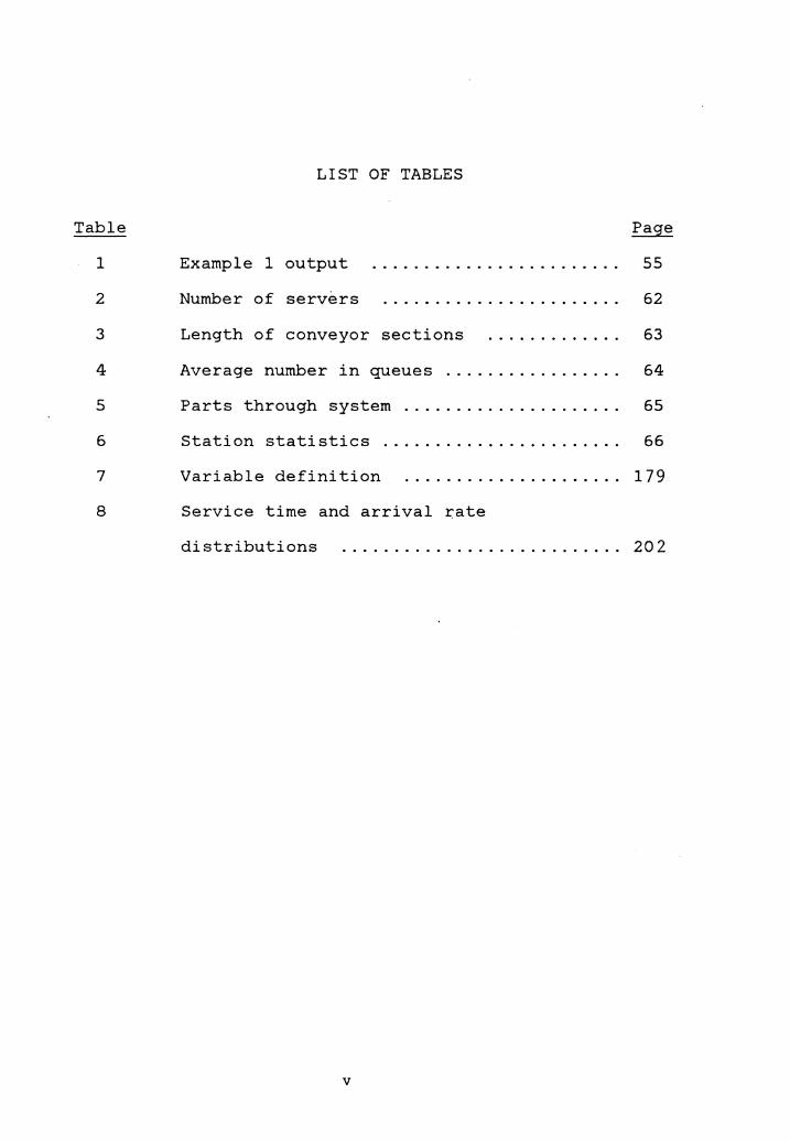
LIST OF TABLES
Example 1 output
Number of servers
Length of conveyor sections
Average number in queues ................ .
Parts through system .................... .
Station stati sties ...................... .
Variable definition
8 Service time and arrival ~ate
distributions
v
Page
55
62
63
64
65
66
179
202
Figure
1
2
3a
3b
3c
3d
3e
3f
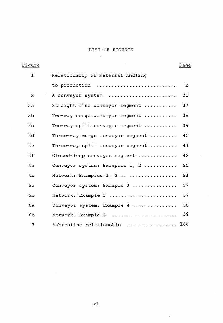
LIST OF FIGURES
Relationship of material hndling
to production
A conveyor system
Straight line conveyor segment
Two-way merge conveyor segment
Two-way split conveyor segment
Three-way merge conveyor segment
Three-way split conveyor segment
Closed-loop conveyor segment
2
20
37
38
39
40
41
42
4a Conveyor system: Examples l, 2 ..........• 50
4b Network: Examples 1, 2 . .. . . . . . . . . . . • . . . . . • 51
Sa Conveyor system: Example 3 ............... 57
Sb Network: Example 3 . . . . . . . . . . . . . . . . . . . . . . . 57
6a Conveyor system: Example 4 ............... 58
6b Network: Example 4 ....................... 59
7 Subroutine relationship 188
vi
Chapter 1
INTRODUCTION
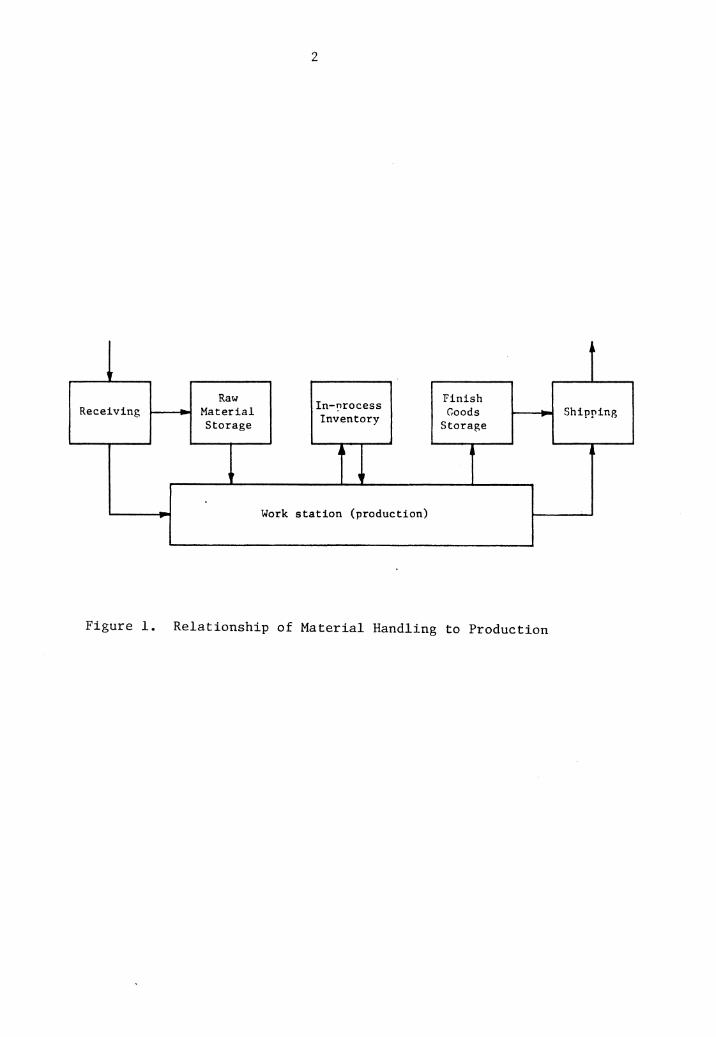
A typical manufacturing facility contains work sta-
tion( s), storage, and receiving and shipping linked by a
material handling system. The simplest manufacturing facil-
ity consists of a receiving dock, service station, and ship-
ping dock (Figure 1). The movement of parts between any two
points in a facility is accomplished using various types of
material handling equipment. The time a unit spends in a
facility is dependent on the effectiveness of the material
handling system being used in that facility.
Material .handling is concerned with: motion, time,
quantity, and space [SJ. Moving material in the most effi-
cient manner, controlling the prqduction time, satisfying
the demand for the manufacturing processes, and utilizing
the available space efficiently are the basis of efficient
material handling.
The material handling system to be used becomes criti-
cal as a business grows. The design and selection of a
material handling system cannot be overlooked if economic
manufacture is desired. Material handling directly affects
the production in terms of manufacturing costs, product
quality and flow, and product traceability. A properly
designed material handling system can reduce costs, increase
1
2
.
Raw Finish Receiving Material In-i:irocess Goods - Shipping
Storage Inventory Storage
,, I
. Work station (production)
Figure 1. Relationship of Material Handling to Production
3
capacity, and improve working conditions. Increased capac-
ity may result in better space utilization, improved layout,
and/or higher equipment utilization. In the past, material
handling costs have been reduced which usually reduced pro-
duction costs. This trend is declining. In some companies,
the material handling cost may be as much as 80-90% of the
labor cost (37).
A variety of material handling equipment is used in
industry. A combination of several types of this equipment
usually make up a material handling system. Apple (5) clas-
sifies different handling equipment under three main types
as:
1. Conveyors.
2. Cranes and Hoists.
3. Industrial trucks.
There are sub-classifications under each. Material handling
systems in operation today are combinations of several types
of equipment which are generally categorized as:
1. Fixed-path handling equipment.
2. Limited area handling equipment.
3. Mobile equipment. (52)
Conveyors, storage/retrieval systems, and monorails are a
few types of the first class. Examples of limited-area
equipment include cranes and hoists while the variable path
equipment covers all forms of industrial trucks and perhaps
towline systems.
4
ADVANCES IN MATERIAL HANDLING SYSTEMS-COMPUTER CONTROLS IN
MATERIAL HANDLING
During the last two decades, material handling systems
have advanced technologically in an extraordinary fashion.
These advancements have contributed significantly in ware-
housing in terms of automation and design. With that trend,
attention is now also being given to processing areas
(actual assembly areas). It is apparent that some trends
have developed. For instance:
1. Automatic and remote controlled equipment,
2. Handling integrated into processing,
3. Handling systems replacing mechanization of indivi-
dual handling tasks,
4. Communication capabilitie~ integrated into equip-
ment,
5. High speed, large capacity, flexible, and better
controlled conveyors,
6. Cranes with remote, and electric or computer con-
trol,
7. Unit handling, and
8. Use of robots. [5]
With the trend toward more sophisticated controls, use
of computers, and microprocessors that diagnose their own
troubles, and progress in other aspects of hardware and
5
applications, better ways for material handling continue to
offer improved operations [ 22] . The trend is toward more
simplified, yet more sophisticated, controls.
Material flow and the optimization of the handling
equipment are the primary functions of the controller today.
These computers respond very quickly to operation require-
ments such as the storage and retrieval of parts, sortation,
transportation, and tracking of every part in the system.
Computer applications have contributed to the advent of
Automatic Storage and Retrieval Systems (ASRS). An ASRS is
an automated warehouse with the storage and retrieval of
parts done either partially or completely automatic. Sto-
rage cells or shelves are used to store parts. Computer
controlled cranes, self-guided stock or order selectors are
used to accomplish the job of storage and retrieval. The
position of each type of part and their quantities are
stored in the memory of the computer. Space has always been
of major concern, and now narrow aisle concepts and use of
guided industrial trucks have shown improvement in space
utilization. The hardware consists of two major parts: 1) A
mini-computer system with disks and tape data storage, video
display terminals and printers, 2) a data terminal that can
be mounted on a guided vehicle. A dual processor would
offer unique security, reliability and data integrity capa-
bilities of substantial values to any warehousing operation
6
[62]. By means of advanced telecommunication technology,
warehouse personnel can remain in constant communication
with the computer system from anywhere in the warehouse.
Carousels are usually used where space is a constraint.
Shelves or bins are used to place parts in this "mini-ware-
house". These multi level bins rotate along a fixed path.
Each part may have a fixed location of storage. Storage and
retrieval of parts is partially or completely automatic.
The location and guanti ties of parts are stored in the
memory of the computer. The storage and retrieval process
is performed by rotating and bringing the desired bin to a
loading/unloading station. Carousels are also being used in
manufacturing environments. Work stations are located
around the carousel so operators have· easy access to the
parts.
Several systems are available for part identification
and tracking. Magnetic and optical sensors, or decoders,
are commonly used for reading identification labels. Pr in-
ters are used to print the labels. Many systems are also
capable of handling inventory and order-entry transactions,
which adds a new dimension to inventory control or the sta-
tus of an order being picked.
In the area of receiving, a software module enables the
system to capture all material as it is taken from the
receiving dock. A radio data terminal is used to identify
7
quantity and storage location of the material. This type of
receiving handles material that does not need individual
tracking [ 62] .
For material flow within the shop, computer controlled
conveyor systems are commonly used. Parts are automatically
moved from work center to work center throughout the system
on a prescribed route. Cartrack systems are also becoming
available and very soon will compete with conveyors. Mono-
tonous and dangerous handling tasks are easily performed
with this equipment.
Computer controlled, robot-like, variable path indus-
trial vehicles generally identified as Automatic Guided Veh-
icles (AGV) will be a major part of future material handling
systems. Currently, AGV systems are primarily used in ware-
housing environments [37).
Automated material handling systems have also contri-
buted in the development of Flexible Machining Systems
(FMS). An FMS consists of a group of work stations linked
by an automated material handling system. Work stations are
usually NC machines. This integrated system is computer
controlled. An important feature of an FMS is that it can
process a variety of different part types simultaneously at
the various work stations.
8
CONVEYORS
There are hundreds of types of material handling equip-
ment and more are being invented every day. It is estimated
that presently there are:
240 types of conveyor,
60 types of trucks and vehicles,
100 types of cranes and hoists,
70 types of containers and racks, and
100 types of auxiliary equipment. or
570 types of material handling equipment [S].
In this section some of the common types of conveyors
are described.
Apple [ 5].
Many definitions have been adopted from
1. Belt Conveyors. An endless fabric, rubber, plastic,
leather, or metal belt operating over belt idlers or sliding
bed for handling materials, packages, or objects placed
directly on the belt. Mesh belts are commonly used in food
processing plants. Flat, portable, and troughed are three
types of belts. Belt conveyor is used for assembly lines,
elevate or lower obje~ts.
2. Bucket Conveyors. Gravity discharged and pivoted are
two types of conveyors of this class of conveyors. Buckets
attached between two endless chains which operate in suita-
9
ble guides or casing in horizontal, vertical, inclined, or a
combination of these paths over drive, corner, and take-up
terminals. Used for heavy and bulk material, and also for
wet and greasy material.
3. Cable conveyors. Overhead Tramway is used when space
is a constraint. Hooks are attached to wheels which move on
a rod.
4. Chain Conveyors. A variety of conveyors fall under
this category. Apron, arm, car type, flight, pallet, roll-
ing, trolley are just to name a few, capable of handling
almost any material.
5. Gravity Chute. A slide
objects as they are moved from
shaped so that it guides
one location to another.
Used for inter-flow and inter level moves.
6. Pneumatic Conveyors. Pipeline, air-activated grav-
ity, and tube are examples of this class of conveyors. Used
for dry material, storage of bulky material, and extra
safety.
7. Roller Conveyors. Mostly used among all types of
conveyors. Supports the load on a series of rollers, turn-
ing on fixed bearings, and mounted between side rails at
fixed intervals. Distance between rollers is dependent on
the size of the object moved. Some example of roller conve-
yors are:
a. Accordian
b. Gravity
10
c. Live
d. Portable
e. Spiral
8. Screw Conveyors. Conveyor consists of a continuous
or broken-blade helix or screw fastened to a shaft (pipe)
and rotated in a trough so that the revolving screw advances
the material.
9. Vibrating Conveyors. A trough or a tube flexibly
supported and vibrated at a relatively high frequency and
small amplitude to convey material (used mostly for hot
objects and gaseous materials).
10. Wheel Conveyors. Gravity, live, and spiral are
three types of this class of conveyors. These conveyors
support the load on a series of skate-·like wheels, mounted
on common shafts in a frame or on parallel spaced rails, and
with the wheels spaced to accomodate the size of the load to
be carried (very similar to roller conveyors).
11
ADVANCES IN CONVEYOR SYSTEMS
Conveyor systems technology has advanced tremendously
in the last decade. Photoelectric sensors and programmable
controllers of the fiber-optic type are used in conjunction
with conveyors for assembly line production. Line shaft
conveyors and conveyors with the capability to make 90
degree turns are playing an important role in live roller
technology. Different types of mechanisms are available to
powerize a conveyor line. Powered accumulating conveyors
which can automatically separate products are also availa-
ble. Accumulating conveyors are used in industry where pro-
ducts must not make any contact with each other. This is
the only type of material handling equipment which can be
used in a 'super clean' electronic industry where any con-
tact of metals generates enough particals to damage the pro-
duct. The electronic industry was probably the last indus-
try introduced to automated material handling.
12
PLANNING FOR A MATERIAL HANDLING SYSTEM
An analytical approach is usually taken in the search
for a solution to the material handling problem. It is
sometimes called the engineering approach. While systemat-
ics may vary, a pattern similar to the following does exist
in most approaches:
1. Identify the problem and the objectives.
2. Determine and collect the appropriate data.
3. Develop alternative solutions.
4. Evaluate alternatives and make a decision.
5. Implement the solution and follow-up for improve-
ments.
Many approaches have appeared in various texts and papers;
but probably, the best and most widely applied approach is
systematic handling analysis (SHA), developed by Muther and
Haganas (59]. Bascially SHA consists of:
1. A framework of phases which organize the project
work.
2. A pattern of procedures to develop material han-
dling plans.
3. A set of conventions.
If these methodologies are applied properly, an effective
solution to a material handling problem can be found.
Unless properly applied more problems and erroneous results
may be obtained.
13
Some of the more common graphical techniques used for
the analysis of material handling problems, and to determine
the relationships between operations, criticality of an
operation, flow of product etc. are given below:
1. Operation Process Chart
2. Flow Process Chart
3. From-to Chart
4. Flow Diagram
5. Critical Path Method
Details on these and others may be found in texts on plant
layout, facilities planning and motion study [ 7, 50, 53,
83].
Another family of techniques is used
alternatives and is usually referred to
Techniques. These are more mathematical
for evaluating
as Quantitative
and operations
research-oriented procedures. Most of these techniques
guarantee a near optimal solution and are divided into these
categories:
1. Deterministic
A. Linear systems
B. Non-linear systems
2. Probabilistic
Some of these techniques will be discussed briefly. It is
very important that a proper technique is chosen and used
correctly.
14
1. LINEAR PROGRAMMING
Linear programming is very frequently used to determine
the best allocation of resources available to accomplish an
objective. The functions expressing the relationships bet-
ween variables must be linear. Linear programming can be
applied to almost all material handling systems. Thompson
[ 85] modeled a scheduling problem as a linear programming
problem.
Integer progamming, transportation programming, and
assignment models are important classes of general linear
programs.
A. INTEGER PROGRAMMING. A special case of linear pro-
gram where variables must be integers. Special cases when
only certain specific variables must be integers (called
mixed-integer program) can also be handled. The model quar-
antees an optimum solution. Phillips and Lytton [66] solved
a decision problem using integer programming.
B. TRANSPORTATION PROGRAMMING. A class of integer pro-
grams is transportation models. Transportation algorithms
are used to minimize the cost of distributing a commodity
from one point to another point. The supply and demand, at
each source and destination are known. This model was
developed to support warehouses and find the best schedule.
15
Restriction of shipment only from a source to destination
and not the other way around may not be realistic.
C. ASSIGNMENT MODEL. Problem of assigning n jobs to n
machines, usually known as the assignment problem, is
another class of integer programs. This is a very useful
technique in layout problems. Problems with dependent
machines are unsol veable. Problems with unequal jobs or
machines can also be handled easily. Aly and Litwhiler [3]
developed an allocation model using this technique and
applied to the public sector.
D. TRAVELING SALESMAN PROBLEM. A special case of
integer program involves finding an optimal route is known
the traveling salesman problem. Each location or facility
is to be visited only once and route must terminate at the
point of origin. No backtracking is allowed. Gensch [27)
applied this technique to solve a static time time-con-
strained scheduling problem.
2. DYNAMIC PROGRAMMING.
Dynamic programming is new among these mathematical
techniques and is designed primarily to improve the computa-
tional efficiency. The basic idea of the technique is to
decompose the problem into smaller subproblems. The dynamic
programming approach changes one problem in n variables into
n problems, each in one variable. The problem is solved in
16
stages and a decision is made at each stage. It is applied
to network routing problems, production scheduling, etc. It
has advantages over conventional procedures in solving mul-
tistage decision problems. Rosenman and Gero [ 78] used a
dynamic programming approach to solve design problems.
3. QUEUEING THEORY
Queueing models account for the random flow in a sys-
tem. Wai ting line or queueing theory assumes parts enter
the system at some rate, move through different service
channels where they are serviced in the fashion in which
they are ordered, and then terminate. The arrival and ser-
vice can be probabilistic. Most of the models make an
assumption of Poison arrival rate and service rate which is
not very realistic. Greshwin and Berman [28] analyzed
transfer lines using Queueing Theory techniques. Solberg
[ 81] developed "CAN-Q" to analyze flows through material
handling systems.
4. CONVEYOR THEORY
Morris [53] classifies conveyors into four categories:
A. Constant speed, irreversible conveyors (open-loop)
B. Operator controlled, reversible conveyors (open-loop)
C. Power and free systems (open loop)
D. Closed-loop, irreversible, continuous operating system.
17
Open-loop systems can be modelled mathematically by using
previously described techniques. Closed-loop system are not
feasible to be described mathematically. Conveyor theory
will be discussed later in the literature review (Chapter
3).
5. SIMULATION
It is always helpful to know how a system is going to
work before its implementation. It is normally too expen-
sive and time consuming to experiment with full scale sys-
tems. Simulation is the tool most often used in making
decisions about the performance of a potential solution.
Simulation cannot guarantee optimality, but the best practi-
cal solution can be found. Many simulation models have been
developed to analyze particular systems [10, 24, 79, 84].
Maxwell [ 44] criticizes these techniques by, "Simula-
tion has been and will continue to be a prime approach to
the problems an industrial engineer, involved in material
handling, faces. Optimization techniques based upon linear
programming (especially flow networks since they capture
inventory relationships) increasingly offer the potential
for avoiding a simulation effort. Queueing approaches
require further development, and most importantly empirical
verification."
Chapter 2
PROBLEM STATEMENT AND OBJECTIVES
Perhaps the most critical step in planning a material
handling system is the evaluation of a proposed system
design. Evaluation of a facility layout, the routing and
scheduling of an AGV system, or the design of a conveyor
system are not easy tasks; but it is advantageous to know
how a particular design or configuration will operate and
perform before it is implemented. Among material handling
equipment, conveyor systems are employed universally (per-
haps more than any other type of material handling equip-
ment). In evaluating the performance of conveyor systems,
design and operational problems are two major areas of
interest for an analyst. These two problems are inseparable
and should be studied together.
There are a number of evaluation techniques (Chapter
1), and it is very important that a proper methodology is
applied to avoid incorrect results and further problems. A
conveyor system, if it meets the objectives under the const-
raints imposed, is said to be operating satisfactorily. An
objective can be in terms of cost, profit, space, through-
put, etc. Additionally, there may be some constraints,
i.e., space, monetary, etc. A mathematical model may seem
to be the easiest way to analyze the problem but is gener-
18
19
ally difficult to do in the case of a complex conveyor sys-
tern. The difficulty encountered is that the conveyor is
part of a large system. The system includes equipment par-
ameters as well as such considerations as spacing, waiting
space allowances, and sequencing of loading and unloading
stations etc. It is also extremely difficult to handle the
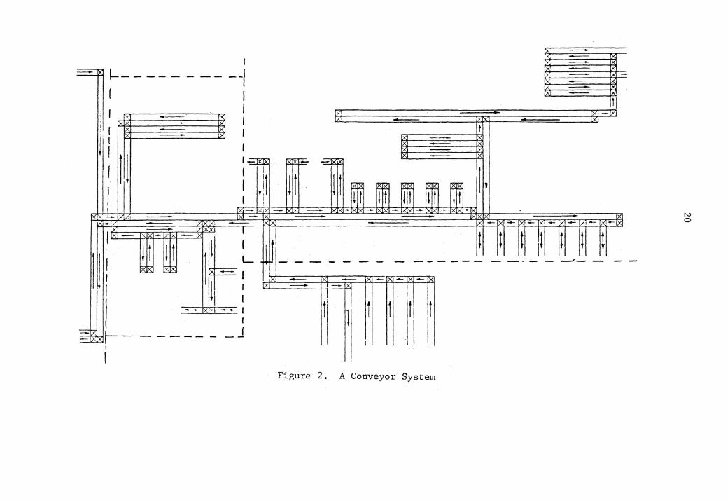
random variables in mathematical models. The layout shown
in Figure 2 is very complex. It includes straight line con-
veyors as well as recirculating or closed loop conveyor sec-
tions. To model this layout as a mathematical program and
include all details may not be possible. Solving this system
to obtain a performance measure may even be a larger prob-
lem.
Perhaps the best way to judge the merit of a particular
design or configuration
[ 9] . Simulation provides
is by simulating its performance
feedback on the present concept
and can be used to make revisions toward a better design.
Unlike other mathematical programs, it is much easier
to include randomness of variables and other detail in a
simulation model. Discrete, continuous, or both types of
material flows can be handled easily. Recirculation and
storage of parts can also be included in the simulation
model.
In modeling continuous systems where one is concerned
with time-dependent variables, general purpose languages
such as BASIC and FORTRAN tend to be used most of the time.
I ~. - !)
)'" - )<
~x !---- -- - - -- --1 X' - x ' - :x -x - " - )
r I XI - :,,.
:1 ' x I t I
1>1 f)(I -1Y -- f'<I I ,, - XI IXI I x !XI ,, I x - TYi I t
j : 1; - :x1 lv"I -~ I)(
I lx'l - IX [)(j - , IX
I =tK!8 l'XT - x ~~~ ~~
( I I
. r I 1 !1 1 t l t ~~ [8~ ~~ ~~ r8::8 I I I I i ! it i f i t i t I I
I IX•- X. IY. - IVI>'. - •Y•Y - y v -CV v - '"" - y - x-rx
IX " _,__ IYL/1 - !xi - > IX lX1 x _./: - v, - " x -"- IX - ·x -- IX1 ~ Y -r/1 x -rXl
xi - I/ y I
it ti 11x1 - '<1x - :YIX IX
~~ t t t t t ! 1 l t ill l I - - - - - - - - ------ - - ... - - ___,_ - -
~18: Zt8 ! I I
ll1 : ,x - :x - x-><-1x-iX'
I IY - - )(
I I
I r ! I t t ! t - )(\":! - I 1 I I I ~x r- - ---- - _J
=-X,;"g -I . I
I
Figure 2. A Conveyor System
N 0
21
An example of a continuous system is a stacker crane, used
in an ASRS, where one may account for the speed and velocity
of the crane. One often must account for hundreds of enti-
ties simultaneously, and monitor changes in their attributes
as they progress through the system. A discrete simulation
language is best used in such cases. Examples of discrete
languages are: GPSS from IBM, SIMSCRIPT from Rand, GASP and
SLAM from Pritsker, and ECSL from the University of Birming-
ham, England [9].
OBJECTIVES
The objective of this research is to develop a simula-
tion package to study and analyze conveyor systems. There
is a need for a large-scale, general purpose simulation
model that can cope with the complexity of actual conveyor
systems. This model should also allow for tradeoff studies
in the design stages as well as the analysis of operational
problems of existing conveyors [ 58]. A simulation model
will be developed to test the performance of conveyor sys-
tems. The objective is two-fold. The first objective is to
develop programming modules which model various conveyor
types and conveyor segments. The second objective is to
compile these modules into a system model to simulate the
proposed layout, shown in Figure 2, as well as some variant
designs. Different conveyor types, for example: belt and
22
gravity roller conveyors, have different operational charac-
teristics and cannot be modeled as one type of conveyor.
Similarly the model must account for different configura-
tions, like straight line and recirculating conveyors.
ORGANIZATION OF RESEARCH
The layout in Figure 2 is very complex and includes
different configurations of conveyor lines. For example:
straight line conveyor, recirculating or loop conveyor,
intersecting and dividing (splitting) conveyors, etc.
Therefore, this layout will be very helpful in testing the
simulation model. A part of this layout is used as an exam-
ple of the application of the simulation model. The simula-
tion study goal is to maximize the flow rates of the product
on the assembly line given the conveyor system layout and
assembly times that are planned for each work station.
Using the example, an analysis to determine any bottlenecks
in the conveyor system is performed. Solutions for elimi-
nating the bottlenecks are also discussed. The analysis
also includes estimation of average contents and utilization
of the conveyor sections, optimization of parts input rate,
minimizing delays, estimating the average flow time, etc.
The assembly line process consists of a group of work
stations through which a product moves in a predefined
sequence. The product is transported via conveyor sections.
23
If the work station storage area is available, it enters the
station. Otherwise, it is recycled on the conveyor sec-
tions. When an assembly (subassembly) is complete, the
assembled part enters the conveyor system and leaves an
opening for another unassembled part to enter that worksta-
tion. All parts are on carriers. Empty carriers are
returned to the point of origin (entry).
The remainder of this thesis is organized into four
major parts. Chapter 3 presents an overview of literature.
Some techniques used in analysis of conveyor systems are
dicussed. This chapter is divided into two areas: 1) Deter-
ministic models, and 2) Probabilistic models.
In Chapter 4, a discussion of how the problem under
consideration may be solved is presented. How the problem
is formulated and modeled is discussed in Chapter 5. Varia-
bles and simulation model are also discussed. Input and out-
put for specific examples is given. A small portion of the
layout shown in Figure 2 is simulated to show how the model
can be used for planning and design purposes.
Chapter 6 contains a brief summary of the research and
a discussion on how the model can be applied to other mater-
ial handling systems in addition to conveyor systems. Future
developements and model expansions are also discussed.
Chapter 3
LITERATURE REVIEW
The design and implementation of a conveyor system is a
very complex process. Evaluating proposed designs is very
critical. Many papers have been published and texts have
been written on the analysis of conveyor systems. In Chap-
ter 1, some techniques for analysis were mentioned. This
chapter gives an overview of the literature and discusses
some research contributions using different analysis techni-
ques. The chapter is divided into two major areas.
1. Deterministic models
2. Probabilistic models
Under these two topics, models with single and multiple
loading and unloading stations (service channels), discrete
and continuous flow of material, and storage areas (banks)
are discussed.
Since the late 19SO's, the birth of conveyor theory, a
lot of work has been done in developing mathematical, net-
work, and simulation models for the analysis of conveyor
systems. Kwo's work [41) on conveyor theory is probably the
earliest work published. He realized the need for analyti-
cal approaches in the study of conveyors. After his appeal
for analytical approaches, a number of papers were published
in the early 1960's [35, 41, 42, 46, 75, 77). Most of these
24
25
early publications were by authors who were also employed as
engineers in industry. Thus, conveyor theory developed from
a concern within industry to develop analytical models of
real world problems [58]. The majority of the work done has
concentrated on constant flow-through conveyor systems.
1. Deterministic Models
One of the very first published works on the analysis
of conveyor systems concentrated on compatibility of the
design of the conveyor with the input and output rates of
parts on the conveyor. Kwo's [41,42] model analyzes a con-
veyor system with one loading station and one unloading sta-
tion, and time-varying patterns of material flow through the
conveyor system. The solution is feasible under some very
restrictive input-output patterns. However, it is not a
general solution procedure. Kwo' s work is considered a
milestone and is further studied by others.
Kwo's model led to a mathematical analysis of the prob-
lem by Muth [54]. He divided the problem into two separate
problems as: 1) continuous loading, and 2) discretely spaced
loading. He also extended his results for single loading
and unloading stations to the case of multiple loading and
unloading stations [ 55, 56]. A difference equation, to
describe material flow along the conveyor, whose solution
yields the conditions under which the conveyor is operable
for general periodic input and output patterns, is used.
26
Moodie, Sadowski, and Hill, Jr. [49] developed an
integer programming model which can be used to determine
optimal (or near optimal) design configurations for unload-
ing of a high speed, mixed product production line. The
procedure is a practical application of integer programming.
The methodology is applied to a conveyor system with one
loading station and multiple unloading stations. Simulation
experiments proved that the results were, in fact, good
designs.
Morgan [51] analyzed the steady-state behavior of two -
link conveyor systems. He considered the systems with
intermediate storage, the mean flow, and the number of car-
riers in queues. For the single carrier in the first link
systems, a set of linear equations are used to determine the
desired values. An approximation method is used for systems
with large number of carriers.
Mitsumori [48] considered a conveyor line with n work
stations. He modeled the system as a mathematical program-
ming problem. Optimization of the conveyor-in sequence is
shown as maximizing the minimum operation time for all work
stations and semi-finished parts.
Ratliff [73] considered a class of production schedul-
ing problems. He discussed how these can be modeled as net-
work flow problems. He assumed that the parts are produced
in batches. He also restricted the cost functions to be
separable and convex.
27
Maxwell and Wilson [ 45] introduced a new methodology
for the analysis of material handling systems. They devel-
oped a network flow model to analyze the flow dynamics of
fixed path material handling systems. The problem is formu-
lated as a cost minimization problem and can also be formu-
lated as a flow maximization problem. Continuous, accummu-
lation, discrete carrier chain, and power and free conveyor
systems can be analyzed by this technique. Even though this
problem has some special characteristics which do not permit
the use of network flow algorithms, it has opened a new area
of research in terms of network flow analysis of material
handling systems.
2. Probabilistic Models
Perhaps the first probabilistic model was developed by
Mayer (46). His model includes n service channels, closed
loop conveyor, and discrete flow of multiple i terns. Al 1
carriers are discretely spaced and are empty when they
arrive at the first station. The conveyor is used to trans-
port the uni ts produced from the workstations to the next
stage. Units are placed in carriers as they are finished.
A nearest available carrier is selected, otherwise, the unit
is placed on the floor. He conducted the analysis with car-
rier capacity of one, and two units. White (86) considered
the general case of a carrier with capacity of x units. He
28
defines the design parameters and indicates how the optimum
values of these parameters can be determined. In addition
to Mayer's model, Morris [53] includes multiple loading and
unloading stations. A conservation of flow approach was
employed to develop the performance measures for the system.
His model was validated by White and Woodbury [ 87] using
simulation.
Some researchers have concentrated on individual work
stations [75,
models of a
76, 77].
loading
They have developed probabilistic
and/or unloading work station. No
delays are allowed. Temporary storage areas are assumed to
avoid delays in loading/unloading operations. The research
focused on the effect of various storage and retrieval dis-
ciplines on production. Beightler and Crisp, and Reis, Bren-
nan, and Crisp [8, 74] modeled a single work station as a
Markov process to analyze the effect of various storage and
retrieval disciplines on the in-process storage require-
ments. [ 8] assumed stationary Bernoulli arrivals but Crisp,
Skieth, and Barnes [19) later proved using simulation that
this assumption could not be validated.
Queueing theory has also been used by many in analyzing
conveyor systems. Disney [23] formulated the two unloading
stations conveyor system as a multichannel queueing problem.
Pritsker [69] generalized Disney's work tom unloading sta-
tions. Disney assumed M/M/m queue, but Pritsker considered
29
M/G/m and D/M/m queues. Pri tsker also used simulation to
allow recirculation with storage allowed only at the last
station. Gregory and Litton [31] formulated the case of m
dissimilar work stations and ordered entry with random arri-
vals as a queueing model and showed that in order to minim-
ize the lost uni ts the work stations should be ordered by
descending service rate. Recirculation is not allowed. All
the work quoted in this paragraph addresses queueing systems
and makes an assumption of non-recirculation, which is very
unrealistic [58].
Proctor, Elsayed, and Ragab [71] investigated the
steady-state behaviour of a two-channel ordered entry conve-
yor system. They analyzed the conveyor system both mathe-
matically, using the principles of the ·queueing theory, and
by simulating it. Storage is allowed only at the second
service center. Elsayed and Proctor [25] also investigated
the steady-state behaviour of two and three channel conveyor
systems with n types of Poisson distributed arrivals, and
two different queueing disciplines.
Agee and Cullinane [2] developed an economic model to
determine the optimum number of loading and unloading sta-
tions and conveyor length. The study is based on a single
loading and a single unloading point with multiple loading
(or unloading) stations allowed at the loading (or unload-
ing) point. A nonstationary Poisson process is assumed and
30
blocking could occur only when the conveyor is full. A
transient analysis is conducted using numerical methods.
Muth [57) analyzed a closed loop conveyor system having
a single loading station, a single unloading station, and
discrete, time-varying input and output flows. It is shown
that the output flow is varied less than the input flow with
a suitable decision rule for unloading.
also allowed.
Recirculation is
Perhaps the only probabilistic analysis which consid-
ered not only Poisson but non-Poisson arrivals as well is
carried out by Matsui and Shingu [ 43]. They analyzed and
developed an unloading policy in a conveyor system with
Poisson and non-Poisson arrivals. The policy minimizes
delay time per unit produced. The results also would be
useful in designing other queueing systems.
Buzacott [12) analyzed an automatic transfer line with
in-process storage consisting of two or three work stations.
He performed a Markov chain analysis and studied the effect
of buffer capacity on the production. He also studied the
line without inventory banks [13) and also with the problem
of breakdowns [14).
Phillips and Skei th [ 67] analyzed a conveyor system
using simulation techniques. They included m service chan-
nels, and recirculation and storage at each channel. This
model was also used to validate the results of Pri tsker.
31
Gourley and Terrell [ 29, 30] developed a modular general
purpose simulation model to study constant-speed, discretely
loaded, and recirculating conveyors. The model is extended
by Chen and Terrell [17] to include multiple loop conveyor
systems which service multiple floors.
GERT and queueing theory is applied together in an ana-
lysis of a conveyor system by Ohta [63]. Service time dis-
tributions are bounded in the discrete conveyor model. No
storage is allowed at the work stations and there is no
recirculation. The model is described by states with Marko-
vian property. The model provides important information in
the system design.
A queueing network analysis program by Solberg [ 81],
CAN-Q can be used to analyze the network flow in a conveyor
system. This evaluation program models the system as a net-
work. Nodes may represent work stations and arcs may repre-
sent flow of parts.
Considerable amount of work has been done in developing
simulation packages for the analysis of production lines.
Possibly the two most significant efforts are by Illinois
Institute of Technology Research Institute [l], and by Phil-
lips, et al [68]. [68] developed Generalized Manufacturing
Simulator (GEMS). Even though it is not specifically
designed for production line analysis, one can represent the
system as a network and apply GEMS. GEMS also requires user
32
to learn modeling in order to use it. On the other hand the
Generalized Assembly Line Simulator (GALS) by [l] is specif-
ically developed for the production line analysis and it
does not require the user to understand any computer lan-
guage or network modeling technique. The user only inputs
necessary parameters in order to execute. GALS, however,
has a drawback that it does not handle material handling
component of production line.
Chapter 4
SOLUTION METHODOLOGY
There are about 240 types of conveyors available today.
Developing programming modules for each and every conveyor
system may not be an easy task and will certainly not be an
efficient way to model these systems. Also, organizing and
keeping track of these many modules in a model may create
problems. A solution to the problem is to categorize the
conveyor types to reduce the programming effort as well as
the compiling effort of the modules into a system model.
A general-purpose model is applicable to many different
conveyor system designs. There are a large number of sys-
terns which differ in design, making it impossible to develop
simulation modules for each separately. A system is made-up
of many conveyor segments. If systems are decomposed into
smaller segments (modules), there will probably be very few
segments with significantly different characteristics.
Developing modules for a few segments and then putting them
together to make-up a system is much easier than developing
separate modules for individual systems.
To summarize the above, as many conveyor types as pos-
sible are classified into as few of classes as possible.
This simplifies the problem of developing a programming
module for each conveyor type. Conveyor systems are broken
33
34
down into smaller conveyor segments, and simulation modules
for these segments are developed. This reduces the problem
to developing modules for a few conveyor segments rather
than the entire systems.
CLASSIFICATION OF CONVEYORS
Conveyors can be classified according to many different
criteria. In this study, conveyors are classified according
to their operating characteristics. Conveyor types fall
into the following categories:
1. Continuous Flow (e.g. Gravity chute)
2. Discretely-spaced (e.g. Belt conveyor)
3. Discretely-spaced Fixed Cycle (e.g. Screw conveyor,
drag-line)
Some of the characteristics of these three classes are
described.
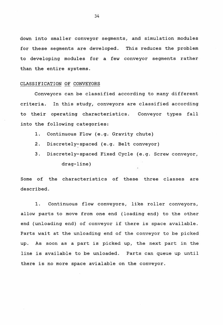
1. Continuous flow conveyors, like roller conveyors,
allow parts to move from one end (loading end) to the other
end (unloading end) of conveyor if there is space available.
Parts wait at the unloading end of the conveyor to be picked
up. As soon as a part is picked up, the next part in the
line is available to be unloaded. Parts can queue up until
there is no more space avialable on the conveyor.
35
2. Discretely-spaced conveyors, like belt conveyors,
operate in the same manner as the continuous flow conveyors
except that there is some distance between parts. When a
part reaches the unloading end of the conveyor and is not
unloaded, it stops the conveyor and no other part can
advance until the first part is picked up from the unloaded
end.
3. Discretely-spaced fixed cycle conveyors, like
bucket conveyors, operate like the previous class of conve-
yors. The only difference is that parts can only be loaded
at fixed points on the conveyor.
The types of conveyors described in Chapter 1 may be
included in these classes as follows:
Class
1
2
3
Conveyor ~
Gravity Chute
Pneumatic
Roller
Vibrating
Wheel
Belt
Chain
Bucket
Cable
Screw
36
BASIC CONVEYOR SEGMENTS
Although
design, they
many conveyor systems differ in overall
all have common basic segments. In other
words, most systems have the same basic segments. For exam-
ple, the layout shown in Figure 2 has three main areas.
Each is different from the other in overall design, but all
of them have the same basic segments such as straight-line
conveyor, intersecting conveyor, etc.
most basic segments are identified.
In this section the
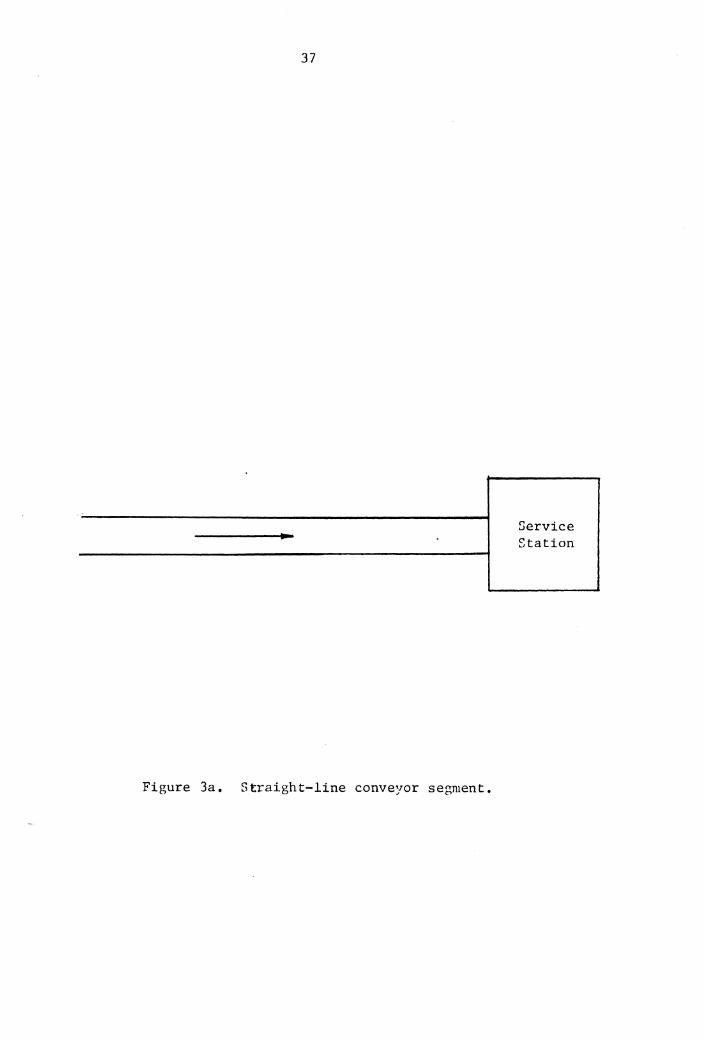
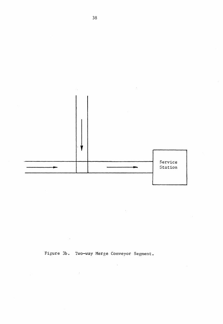
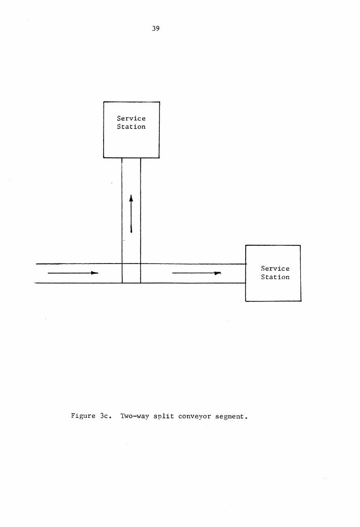
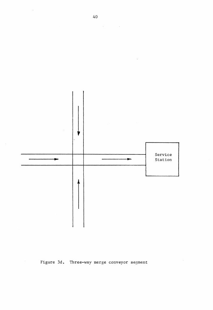
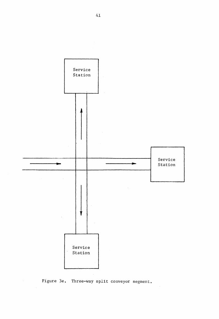
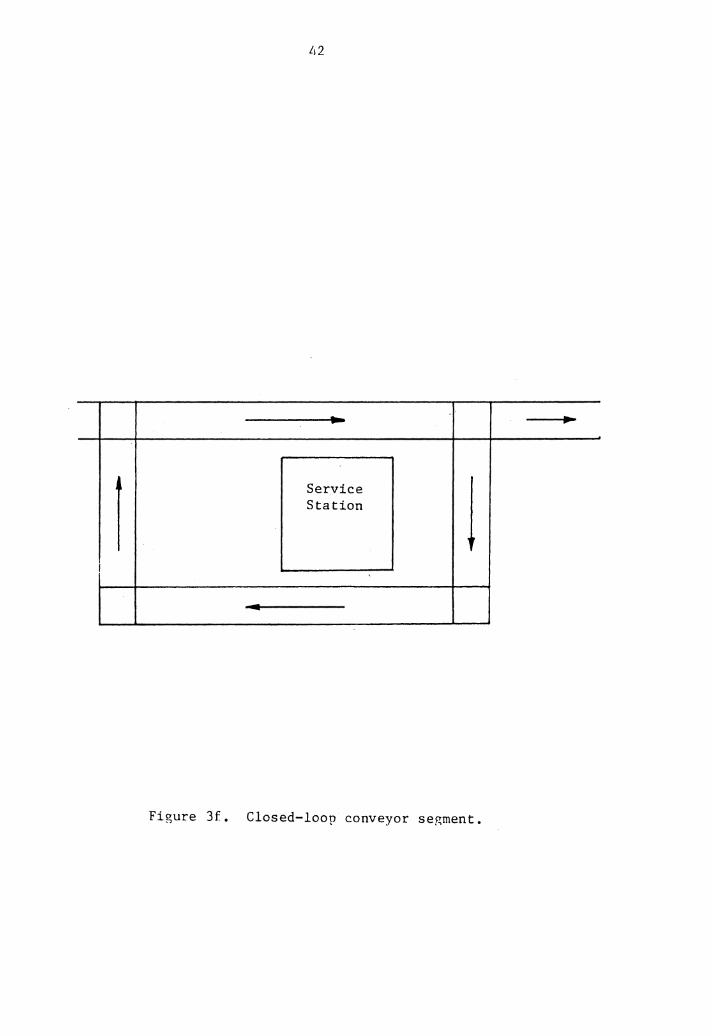
Perhaps the most common and the most basic segment is a
straight line conveyor. Two-way merge and split, three-way
merge and split, arid closed-loop are other segments. These
are shown in Figures 3a through 3f. By arranging these seg-
ments properly, one can design an entire system.
Given the three classe·s and these segments, programming
modules are developed for the feasible combinations. For
example: class 1 conveyors can be used in designing any
segment, but class 3 conveyors cannot be used to design
merging, intersecting, or closed loop conveyors. The feasi-
ble combinations are as follows:
37
Figure 3a. Straight-line conveyor segment,
Service Station
38
• If
Service . Station
Figure 3b. Two-way Merge Conveyor Segment.
39
Service Station
1 Service - -· Station
Figure 3c. Two-way split conveyor segment.
40
,
Service - - Station -
..
Figure 3d. Three-way merge conveyor segment
Service Station
.
Service Station
41
Figure 3e. Three-way split conveyor segment.
Service Station
L~2
...
l Service
l Station
I
.
Figure Jf. Closed-loop conveyor segment.
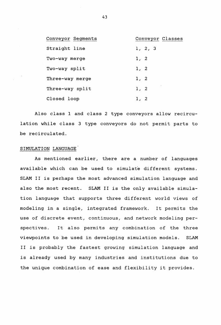
43
Conveyor Segments Conveyor Classes
Straight line l, 2, 3
Two-way merge l, 2
Two-way split 1, 2
Three-way merge 1, 2
Three-way split 1, 2
Closed loop 1, 2
Also class 1 and class 2 type conveyors allow recircu-
lation while class 3 type conveyors do not permit parts to
be recirculated.
SIMULATION LANGUAGE
As mentioned earlier, there are a number of languages
available which can be used to simulate different systems.
SLAM II is perhaps the most advanced simulation language and
also the most recent. SLAM II is the only available simula-
tion language that supports three different world views of
modeling in a single, integrated framework. It permits the
use of discrete event, continuous, and network modeling per-
spectives. It also permits any combination of the three
viewpoints to be used in developing simulation models. SLAM
II is probably the fastest growing simulation language and
is already used by many industries and institutions due to
the unique combination of ease and flexibility it provides.
44
SUMMARY OF PROPOSED METHODS
The objective of this study is to develop a simulation
model to study and analyze conveyor systems. Conveyors are
categorized into three classes. Six segments which differ
in design are the foundations of most of the system designs.
Feasible combinations of conveyor classes and segments are
modeled within a SLAM II framework. These programming
modules are compiled into a system model. This model will
be tested by applying it to variant designs.
Chapter 5
SIMULATION MODEL
This problem can be formulated by using the discrete-e-
vent or network portions of SLAM. The network portion of
SLAM is conceptually easier to use but is not efficient
(computationally) when dealing with larger systems. The
discrete-event portion of SLAM is not as easy to use but
adds flexibility in modeling larger systems. Conveyor sys-
tems can also be formulated by using both portions together.
A decision on which modeling technique to use was made after
testing the ease and flexibility of modeling. It was
decided to formulate the problem using discrete-event SLAM.
MODELING PROCEDURE:
The simulation model is structurally divided into three
sections, each section corresponding to a different class of
conveyors. This simplified the programming efforts and also
made it easier to debug the model. Each section is basi-
cally the same except for a few minor details to distinguish
among the three classes of conveyors.
Conveyor systems are treated as networks. Nodes repre-
sent a merging or splitting point (intersection) and also
the service areas (stations, machines) . Conveyor sections
are represented as arcs. When a part, or entity, enters the
system, it is assigned some attributes which are modified as
45
46
it moves through the system. An entity is assigned its
proper route in terms of the service areas it needs to
visit. The model transforms this in terms of nodes and arcs
in the network.
Dijkstra's shortest path algorithm is used to determine
the path between two stations. This path is in terms of
nodes and arcs in the network, and is assigned to attributes
of an entity.
Basically the model moves parts from conveyor to conve-
yor, and from station to station. There is no major differ-
ence in the concepts of modeling the three classes of conve-
yors. In all three cases, 'look ahead' methodology is
employed. If there is no space on the conveyor, or the sta-
tion, where a part is supposed to go next, it is stopped in
the system. The only difference among the three sub-systems
is the detail required before moving a part. Consider the
following cases when a part needs to move from a conveyor,
or a station to another conveyor or station. The modeling
differences in modeling the three classes of conveyors fol-
lows.
1. A part has just arrived in the system and needs to
go to conveyor 1. If there is no space on conveyor 1, it
will not be put onto the conveyor. It will wait in a file
(queue). For class 2 conveyors, an additional check is made
to see if conveyor 1 is running or not. If not, the part
47
will wait in a queue. For class 3 conveyors, in addition to
the above two conditions, another condition must be met
before the part can be placed on the conveyor. It is
required that the part must wait for a loading point on the
conveyor before a test on the status of conveyor (availabil-
ity of space and working condition) is made.
2. Now consider the case where a part needs to go from
one conveyor 1 to another conveyor 2, which precedes 1. If
the part is not able to go to 2, it stays on 1 and also
blocks the parts following it on 1. For classes 2 and 3,
when this happens, conveyor 1 also stops moving and it
delays the movement.of parts on it.
3. Further consider the case where a part has just
finished service at station 1 and needs.to go to conveyor 2,
which precedes conveyor 1. When the part cannot leave the
station, because of any of conditions given in case 1, it
will stay at the station and will block the server from
serving any more parts. When there is a space on conveyor 2
and if it is functioning, the part which is blocking a ser-
ver will have priority over any other parts on conveyor 1 to
be loaded onto conveyor 2.
4. Consider the case in which a part has reached a
sevice station and needs to be served there. If the server
is busy and recirculation is allowed, it will continue mov-
ing if possible, otherwise it will be stopped. If recircu-
48
lation is not allowed, it will stop there and wait until
served. It will stop the parts following it.
Modeling Assumptions and Constraints.
1. Conveyor speed is constant.
2. Different types of parts are allowed in the system.
A part is different from another part if they fol-
low different routes. All parts, same type or
different types, have the same dimensions (unit
load). It is easier to check how much space is
available on a conveyor by just looking at the num-
ber of parts on the conveyor.
3. All queues are arranged according to first come
first serve priority. Only the priority on service
queues can be changed using SLAM input statements
(discussed later).
4. There is no pre-emption allowed in the service.
5. At present all yields are 100%. There are no bad
parts produced.
6. There may be identical and independent servers at a
station. If two servers at a station have diffe-
rent service times, they should be treated as two
different stations.
7. A service area, or station, has only one queue, and
all servers share that common queue.
49
8. At present, there is only one location for a ser-
vice area.
9. At present, there is only one entrance for a part
type.
10. A node can have a maximum of 4 arcs eminating and
departing. In other words, a node can be linked
with a maximum of 4 other nodes.
11. Service times and interarrival times can be any of
the following type:
a. Constant,
b. Random,
c. Exponentially distributed,
d. Uniformally distributed,
e. Triangularly distributed, ·and
f. Normally distributed.
EXAMPLES:
Small conveyor systems are used to discuss input and
output for the three classes of conveyors and how one can
use the model. Another system is simulated to discuss how
the model can help in designing or improving the design of a
system.
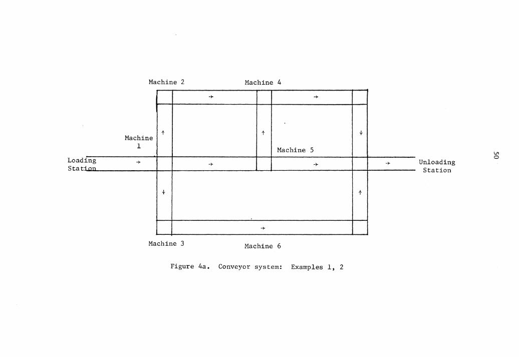
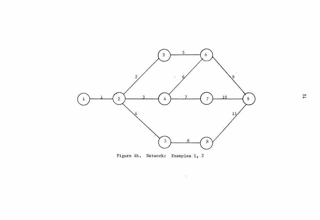
1). A conveyor system, shown in Figure 4a, has six
different stations which serve three different types of
parts. Figure 4b represents the network form of the system.
Load Stat
:lng ; nn
Machine 2 Machine 4
-+ -+
t t Machine
1 Machine 5 -+ -+ -+
+
-+ -
Machine 3 Machine 6
Figure 4a. Conveyor system: Examples 1, 2
+
-+
t
-1
-Unloading Station
\J1 0
':r:!
I-'·
OQ
i:: ti
!Tl
.p.. CT' z !Tl
rt
~
0 ti ~
trj >: PJ El 'Q .....
!Tl
00
Ul
I-' .. N
52
Arc numbers are placed over each arc. How the conveyor sys-
tern is converted into a network is described here.
information about the system is given below.
Also,
Each conveyor section is represented as an arc in the
system. Each station is represented as a node. If a sta-
tion is in the middle of a conveyor section, a node, repre-
senting the station, is dividing the two arcs which repre-
sent the conveyor. In this case, one conveyor is split into
two conveyors. Any junction of two or more conveyors is
also represented as a node. The loading and unloading sta-
tions are also nodes even if the loading/unloading time is
zero.
In Figure 4b, nodes and their description are as fol-
lows:
Node 1 Loading station
Node 2 Machine center 1
Node 3 Machine center 2
Node 4 Splitting point
Node 5 Machine center 3
Node 6 Machine center 4
Node 7 Machine center 5
Node 8 Machine center 6
Node 9 Unloading station
Only node 4 is not considered a station.
53
Input:
Appendix B contains input and output for the examples.
First, consider the input to example 1.
1. SLAM Input. This will not be discussed here. The user
can consult the SLAM manual or text [ 70] . The variables
which are dependent upon the conveyor system are discussed
in Appendix C.
2. MODEL Input. Input to the model is unformated and
described in detail in Appendix C. Limitations on some of
the variables are also mentioned.
Output:
There are three parts of the output. First is the SLAM
echo report. The second is the intermediate results. SLAM
summary report is the third part of the output.
SLAM echo report is basically to check the input data
and SLAM variables. This is explained in detail in SLAM
text [ 70]. Intermediate results will always give statistics
for how much time a unit spends on a conveyor and how many
units are on a conveyor. Average, standard deviat~on, etc.
is printed out.
the formula.
Conveyor Utilization
Conveyor utilization can be calculated by
Ave. number on Conveyor Capacity of conveyor x 100%
54
As can be seen from Table 1, conveyor 1 was utilized
71. 77% in example 1.
Conveyor Utilization = 2.153 x 100% 3.000
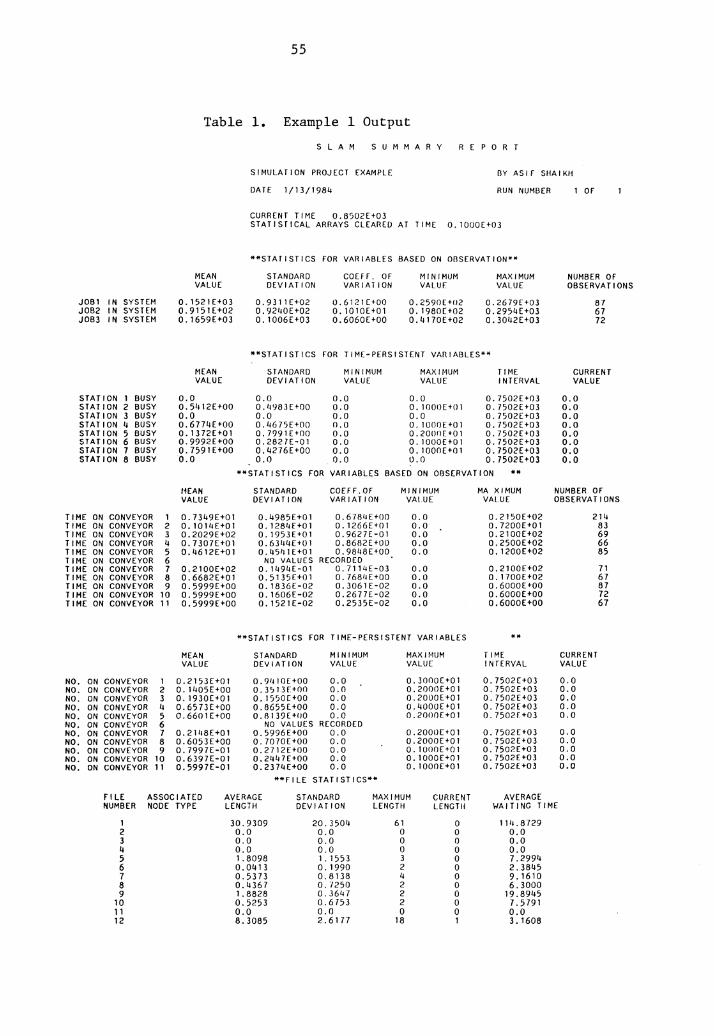
Table 1 summarizes the output of example 1. The SLAM sum-
mary report provides statistics on how much time each part
of a particular type spends in the system. It also gives
statistics on how many servers at a station are busy. The
user can determine other statistics by simple calculations.
An important part of the SLAM summary report is file
statistics. This indicates how many parts are waiting at a
station and how long do they wait. Consider exaple l; User
may neglect statistics on files l, 2, and 3. File 1 is used
when a part is waiting to move from a station to a conveyor,
or from another conveyor if the node between the two conve-
yors is not a station. Files 2 and 3 are not used for class
1 conveyors. Fi le 4 through the maximum number of user
defined files are used when a part is waiting for service at
a station or while waiting to go to another conveyor which
is not available. The last file, file 12, is of no interest
to the user, it is the event calender.
All this information can be helpful in making design
decisions and evaluting alternatives. This will be dis-
cussed later.
JOB1 IN SYSTEM JOB2 IN SYSTEM JOB3 IN SYSTEM
STATION 1 BUSY STATION 2 BUSY STATION 3 BUSY STATION lj BUSY STATION 5 BUSY STATION 6 BUSY STATION 7 BUSY STATION 8 BUSY
TIME ON CONVEYOR 1 TIME ON CONVEYOR 2 TIME ON CONVEYOR 3 TIME ON CONVEYOR 4 TIHE ON CONVEYOR 5 TIME ON CONVEYOR 6 TIME ON CONVEYOR 7 TIME ON CONVEYOR 8 TIME ON CONVEYOR 9 TIME ON CONVEYOR 10 TIME ON CONVEYOR 11
NO. ON CONVEYOR 1 NO. ON CONVEYOR 2 NO. ON CONVEYOR 3 NO. ON CONVEYOR 4 NO. ON CONVEYOR 5 NO. ON CONVEYOR 6 NO. ON CONVEYOR 7 NO. ON CONVEYOR 8 NO. ON CONVEYOR 9 NO. ON CONVEYOR 10 NO. ON CONVEYOR 11
55
Table 1. Example 1 Output S L A M S U M M A R Y R E P 0 R T
SIMULATION PROJECT EXAMPLE
DATE 1/13/ 1984
llY ASIF SHAIKH
RUN NUMIJER
CURRENT TIME 0.8502E+03 STATISTICAL ARRAYS CLEARED AT TIME 0. 1000E+03
**STATISTICS FOR VAHIABLES BASED ON OllSERVATION•*
MEAN STANDARD COEF F. OF MINIMUM MAXIMUM VALUE DEVIATION VARIATION VALUE VALUE
0. 1521[+03 0.9311[+02 0.6121[+00 0.2590E+o2 0.2679£+03 0.9151[+02 D. 92110E+02 0. 1010E+01 0. 1980[+02 0.2954E+03 0. 1659E+03 0.1006E+03 0.6060E+OO 0.4170E+02 0. 3042E+03
**STATISTICS FOR TIME-PERSISTENT VARIABLES**
MEAN STANDARD MINIMUM MAXIMUM TIME VALUE DEV I AT I ON VALUE VALUE INTERVAL
0.0 0.0 0.0 0.0 o. 7502E+03 0. 51112E+OO 0.4983E+OO 0.0 0.1000E+01 0. 7502E+03 o.o 0.0 0.0 0.0 0. 7502E+03 0.6774E+OO 0.4675E+OO 0.0 0. lOOOE+Oi 0.7502E+03 0.1372E+01 0. 7991E+OO 0.0 0.200()[+D1 D. 7502E+03 0.9992E+OO 0.2827E-D1 0.0 D. lOOOE+OI o. 7502E+03 o. 7591E+oo 0.42l6E+OO o.o 0. 1OOOE+O1 0. 7502E+03 0.0 0.0 0.0 o.o 0. 7502E+03
**STATISTICS FOR VARIABLES BASED ON OBSERVATION **
MEAN STANDARD COEFF.OF MINIMUM MA XIMUM VALUE DEVIATION VARIATION VAlUE VALUE
0. 7349E+01 0.4985E+01 0.6784E+OO 0.0 0.2150E+02 0.101l1E+OI 0. 1284f+O 1 0.1266E+OI 0.0 0. 7200E+01 0.2029E+02 0.1953E+01 0.9627E-01 0.0 0.2100E+02 0. 7307E+01 0.63114E+01 0. 8682E+OO 0.0 0.2500E+02 0.4612E+01 0. 4511lE+O1 0.9848E+OO 0.0 0. 1200E+02
NO VALUES RECORDED 0.2100E+02 0.1494E-01 0.7114E-03 0.0 0.2100E+02 0.6682E+01 0.5135E+01 0. 76811E+OO 0.0 0. 1700E+02 0.5999E+OO 0.1836E-02 0.3061E-02 0.0 0.6000E+OO o.5999E+oo 0.1606E-02 0.2677E-02 0.0 0.6000E+OO 0.5999E+OO 0. 1521E-02 0.2535E-02 o.o 0.6000E+OO
**STATISTICS FOR TIME-PERSISTENT VARIABLES .... MEAN STANDARD MINIMUM MAXIMUM TIME VALUE DEVIATION VALUE VALUE INTERVAL
0.2153E+01 0. 9111 OE+OO 0.0 0.3000E+01 0. 7502[+03 0. 1405E+OO 0.3513F+OO 0.0 0.2000E+OI 0. 7502E+03 0.1930E+01 0. 15~0[+00 0.0 0.2000E+01 0. 7502E+03 o. 6573E+oo 0.8655E+OO 0.0 0.4000E•01 0. 7502E+03 0.6601E+OO O.Rl39E+OO 0.0 0.2000[+01 0. 7502f+03
NO VALUES RECORDED 0. 2 Jl18E+Ol 0.5996E+OO 0.0 0.2000E+01 0. 7502E+03 0.6053E+OO D. 7070E+OO 0.0 0.2000E+01 0. 7502E+03 0. 7997E-01 0. 2712E+OO 0.0 0. I OOOE+O 1 0. 7502E+03 0.6397E-01 0.2447E+OO 0.0 0.1000E+01 0. 7502E+03 0.5997E-01 0.2374E+OO o.o 0. IOOOE+Ol o. 7502E+03
**FILE STATISTICS**
OF
NUMBER OF OBSERVATIONS
87 67 72
CURRENT VALUE
0.0 0.0 o.o 0.0 0.0 0.0 0.0 0.0
NUMBER OF OBSERVATIONS
214 83 69 66 85
71 67 87 72 67
CURRENT VALUE
0.0 0.0 o.o 0.0 0.0
0.0 o.o 0.0 o.o 0.0
FILE ASSOC I A TEO AVERAGE STANDARD MAXIMUM CURRENT AVERAGE NUMBER NOOE TYPE LENGTH DEVIATION LENGTH LENGTH WAITING TIME
1 30.9309 20.35011 61 0 1111.8729 2 0.0 0.0 0 0 o.o 3 0.0 0.0 0 0 0.0 4 0.0 0.0 0 0 0.0 5 1.8098 1. 1553 3 0 7.2994 6 0.0413 0. 1990 2 0 2. 3845 7 0.5373 0.8138 4 0 9. 1610 8 0.4367 0. 7250 2 0 6. 3000 9 1. 8828 0.3647 2 0 19.8945
10 0.5253 0.6753 2 0 7. 5 791 11 0.0 0.0 0 0 0.0 12 8.3085 2. 6177 18 1 3. 1608
56
2). Same conveyor system is simulated but a class 2
conveyor is used.
before.
Output contains the same information as
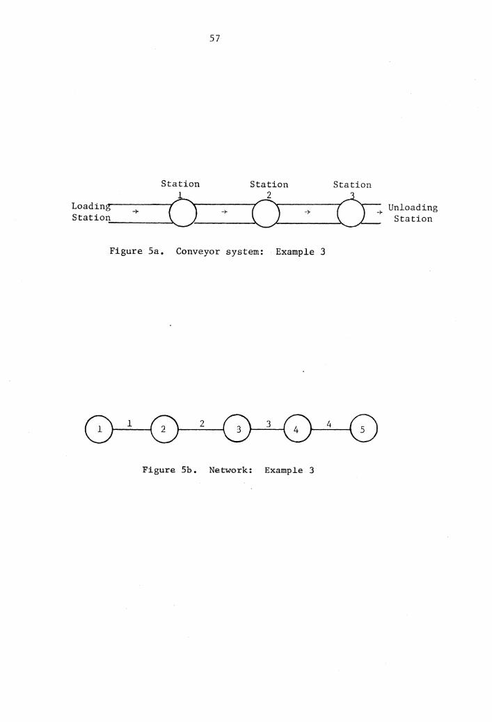
3). Consider a class 3 conveyor system, shown in Figure
Sa. There is a little difference in interpreting the out-
put. File 1 is used for parts waiting to enter the system.
File 3 is used to hold parts while they are waiting to go
from a station to a conveyor. Fi le 2 and 12 are of no
interest to user.
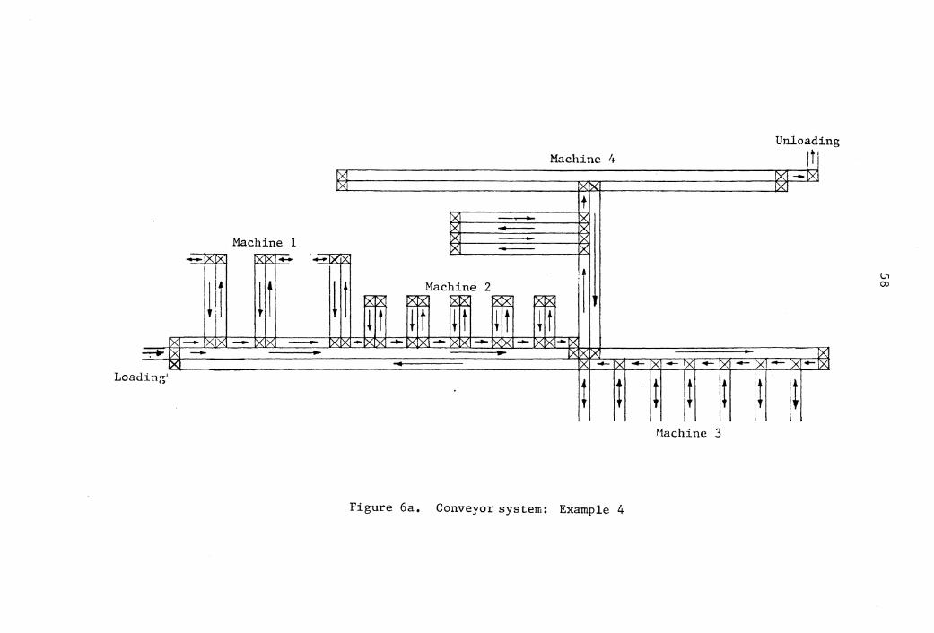
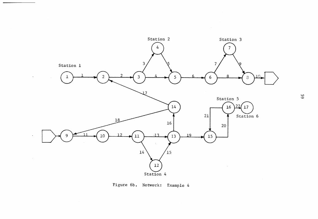
4). This example is to explain how the model helps in
design and evaluaton of alternatives. A part of Figure 2
layout, shown in Figure 6a is used for these purposes. This
is transformed into network shown in Figure 6b.
Since the model only allows single location for a sta-
tion, some adjustments are made in the layout to fit the
model. Multi-located stations are those stations which have
servers at more than one location. Station 2 has three ser-
vers at different places and each serving a different queue.
It is assumed that these servers can be combined at one
location and can be served through one queue. In making
these adjustments, some conveyor sections are oriented
differently than the layout shown in Figure 6a, and some
have their capacity varied. User must also realize that the
accessibility of some servers has also increased since parts
do not travel to another location for service.
Station l
Load in,..------~ Station ______ ,
57
Station 2
Figure Sa. Conveyor system: Example 3
Figure Sb. Network: Example 3
Station
Unloading Station
Machine /} M IYI '>I '\{
t '>t -........- ~
'>t - ~
Machine 1 ){ - ~
x - )( - XIX ~~~ ~~~ I : l · !11 l! l 1
Machine 2 s:~ 8~ ~~ ~~ ~8:
I t I i t i t + t + t IX!-+ 1XIY - XY - Yx ... xv _., x y -- >< y -- xx -- xx -1x
~IYI - - IX xx fXI x ...__
x ---Load
t t
Figure 6a. Conveyor system: Example 4
'x -- I)( -- x- y
t 11 I t t Machine 3
Unloading
Iii IYl -- IXI M
IXI - rx -IXI
t
\..11 00
60
The system is simulated with deterministic and proba-
bilistic inter-arrival and service times. Execution time
difference between the two models (deterministic, probabil-
istic), for this conveyor system, is approximately 2.50 sec-
onds. This may vary with the size of the system being simu-
lated.
Four runs, with probabilistic times, are included in
Appendix B. The output and control variables are discussed
in this section.
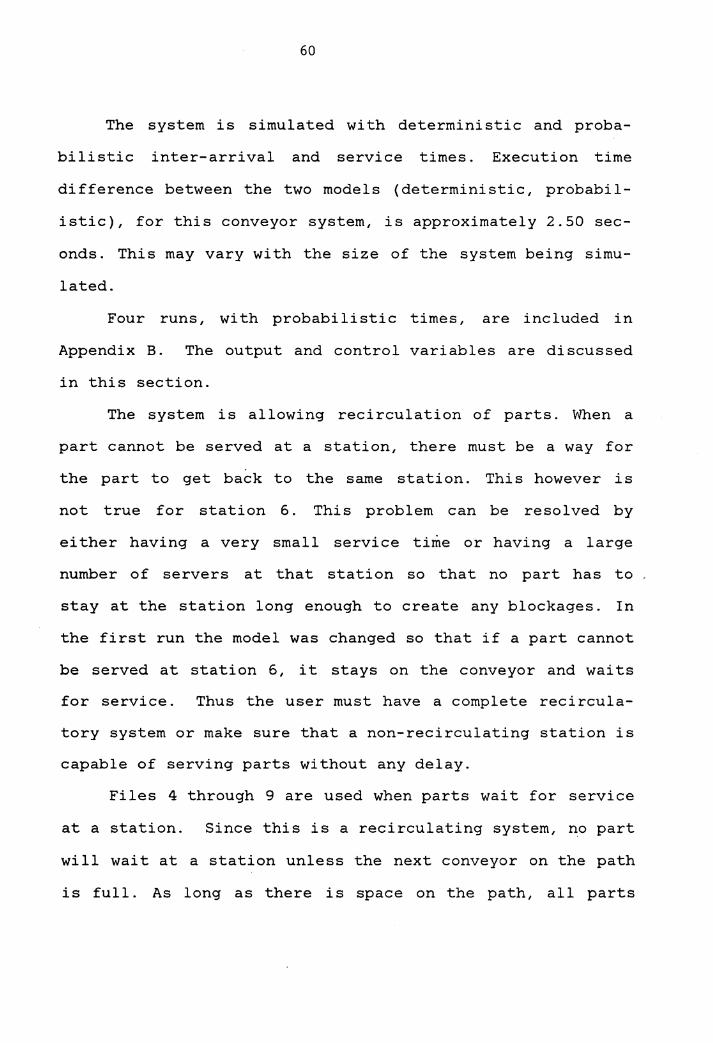
The system is allowing recirculation of parts. When a
part cannot be served at a station, there must be a way for
the part to get back to the same station. This however is
not true for station 6. This problem can be resolved by
either having a very small service time or having a large
number of servers at that station so that no part has to
stay at the station long enough to create any blockages. In
the first run the model was changed so that if a part cannot
be served at station 6, it stays on the conveyor and waits
for service. Thus the user must have a complete recircula-
tory system or make sure that a non-recirculating station is
capable of serving parts without any delay.
Files 4 through 9 are used when parts wait for service
at a station. Since this is a recirculating system, no part
will wait at a station unless the next conveyor on the path
is full. As long as there is space on the path, all parts
61
will continue moving and no entity will be placed in files.
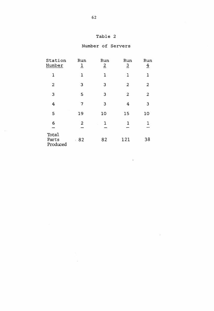
Table 2 lists all the combinations of the number of servers
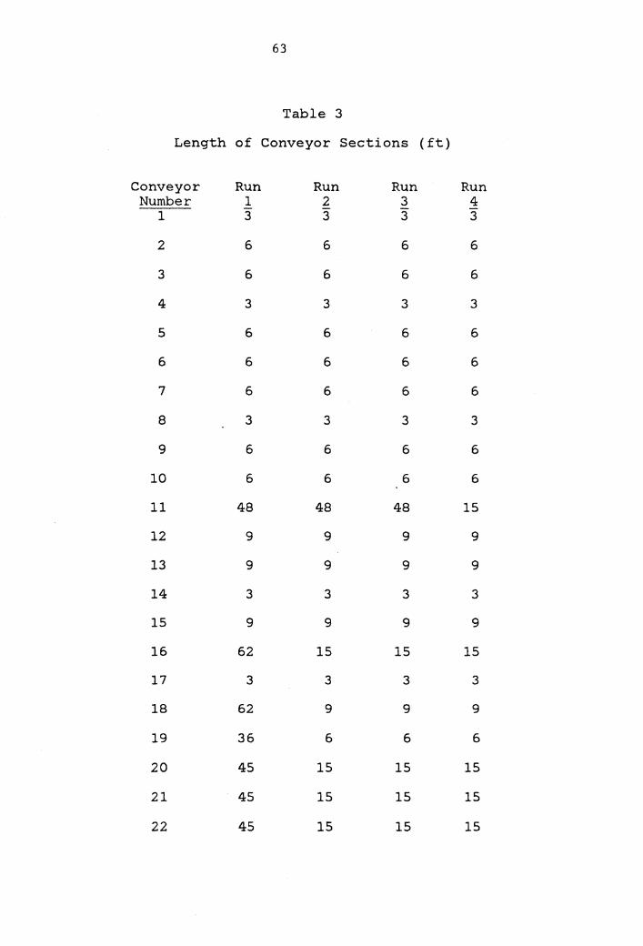
tried. Table 3 lists length of each conveyor section used
in four runs. Table 4 summarizes the average number of
parts in files. As mentioned, run 1 is the only run where
station 6, or file 9, has some entities waiting for service.
This system is never completely full, therefore, no part is
placed in any file (runs l, 2, and 3 only). If a part is
placed in a file, information on how long it waits in the
queue, how many parts are waiting now, average number of
parts waiting, and at the most how many parts are waiting,
etc. is provided in the output (see Appendix B).
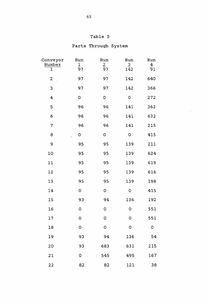
Table 5 indicates how many parts went through different
conveyor sections. Information on how long a part stayed on
a conveyor section is provided in the output (see Appendix
B).
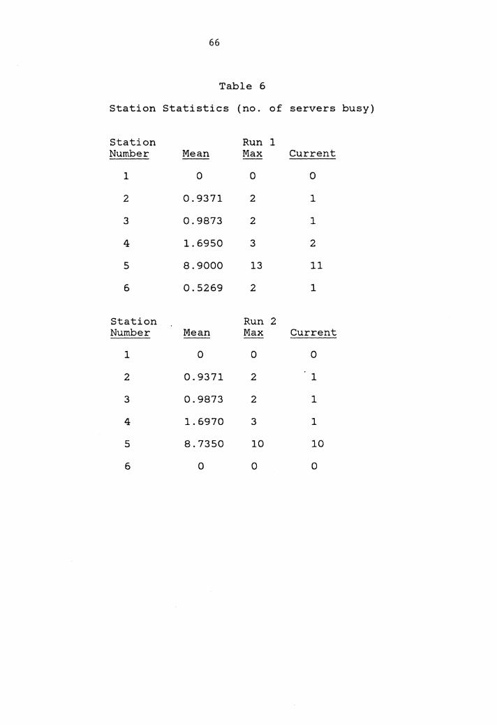
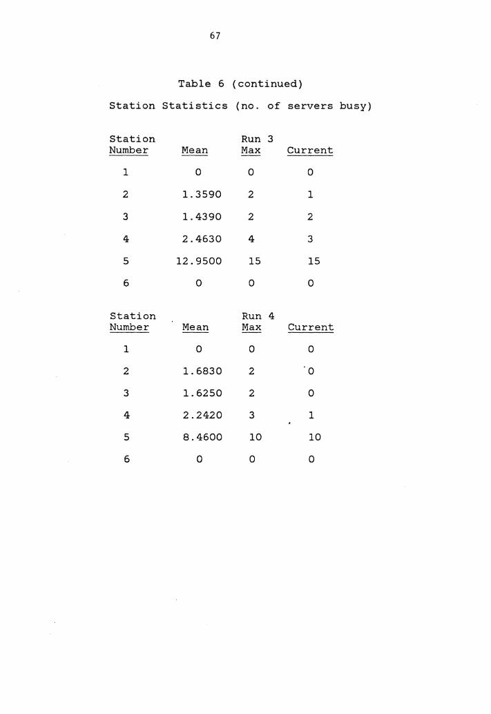
Table 6 indicates average, maximum, and current number
of servers busy at each station.
After the first simulation run, it is clear that no
part had to wait at any station or conveyor section. Every
part went through the system without any delay. Of note, the
same results were obtained when this system was simulated
using a GPSS simulation model. This is good if the designer
wants a system which ,in case of any machine breakdown will
still perform without any delays. On the other hand the
62
Table 2
Number of Servers
Station Run Run Run Run Number 1 2 3 4
1 1 1 1 1
2 3 3 2 2
3 5 3 2 2
4 7 3 4 3
5 19 10 15 10
6 2 1 1 1
Total Parts 82 82 121 38 Produced
63
Table 3
Length of Conveyor Sections (ft)
Conveyor Run Run Run Run Number 1 2 3 4
1 3 3 3 3
2 6 6 6 6
3 6 6 6 6
4 3 3 3 3
5 6 6 6 6
6 6 6 6 6
7 6 6 6 6
8 3 3 3 3
9 6 6 6 6
10 6 6 6 6
11 48 48 48 15
12 9 9 9 9
13 9 9 9 9
14 3 3 3 3
15 9 9 9 9
16 62 15 15 15
17 3 3 3 3
18 62 9 9 9
19 36 6 6 6
20 45 15 15 15
21 45 15 15 15
22 45 15 15 15
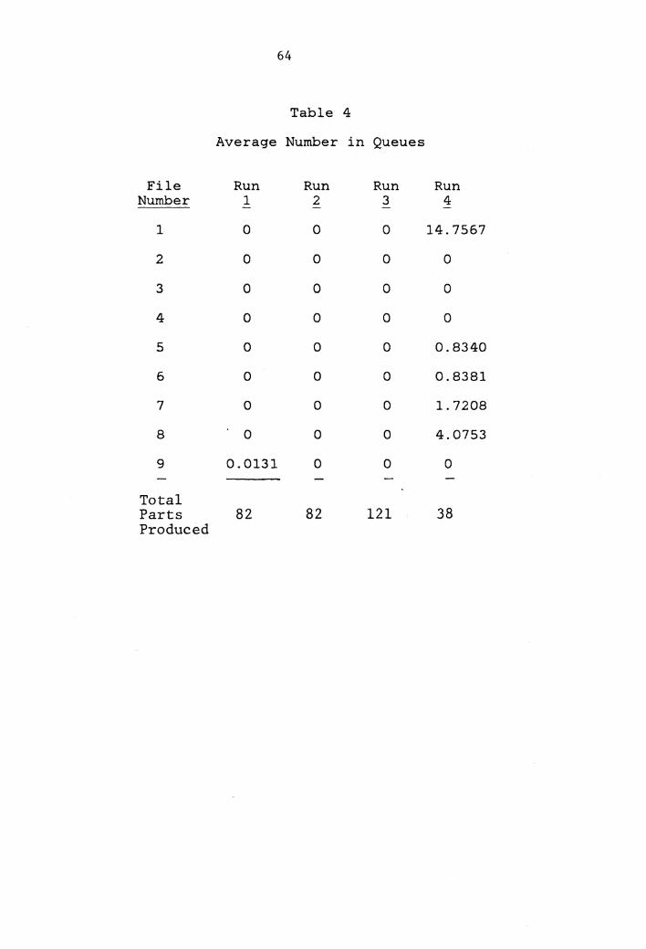
64
Table 4
Average Number in Queues
File Run Run Run Run Number 1 2 3 4
1 0 0 0 14.7567
2 0 0 0 0
3 0 0 0 0
4 0 0 0 0
5 0 0 0 0.8340
6 0 0 0 0.8381
7 0 0 0 1.7208
8 0 0 0 4.0753
9 0.0131 0 0 0
Total Parts 82 82 121 38 Produced
65
Table 5
Parts Through System
Conveyor Run Run Run Run Number 1 2 3 4
1 97 97 142 91
2 97 97 142 640
3 97 97 142 366
4 0 0 0 272
5 96 96 141 362
6 96 96 141 632
7 96 96 141 215
8 0 0 0 415
9 95 95 139 211
10 95 95 139 624
11 95 95 139 619
12 95 95 139 616
13 95 95 139 198
14 0 0 0 415
15 93 94 136 192
16 0 0 0 551
17 0 0 0 551
18 0 0 0 0
19 93 94 136 54
20 93 683 631 215
21 0 545 495 167
22 82 82 121 38
66
Table 6
Station Statistics (no. of servers busy)
Station Run 1 Number Mean Max Current
1 0 0 0
2 0.9371 2 1
3 0.9873 2 1
4 1.6950 3 2
5 8.9000 13 11
6 0.5269 2 1
Station Run 2 Number Mean Max Current
1 0 0 0
2 0.9371 2 1
3 0.9873 2 1
4 1. 6970 3 1
5 8.7350 10 10
6 0 0 0
67
Table 6 (continued)
Station Statistics (no. of servers busy)
Station Run 3 Number Mean Max Current
1 0 0 0
2 1. 3590 2 1
3 1. 4390 2 2
4 2.4630 4 3
5 12.9500 15 15
6 0 0 0
Station Run 4 Number Mean Max Current
1 0 0 0
2 1.6830 2 0
3 1. 6250 2 0
4 2. 2420 3 1
5 8.4600 10 10
6 0 0 0
68
designer can certainly make changes in the system, and still
have a good system (performance criteria is required to make
any judgements). Number of servers can be reduced at some
stations. Some conveyor sections may be eliminated, and
some may be reduced in length. In terms of changes, the fol-
lowing may be said about any system:
1. vary conveyor speed,
2. vary capicity of conveyor sections,
3. vary number of servers at stations,
4. vary input rate, etc.
In this example, one may want to increase the input
rate, reduce the number of servers, and/or reduce the capac-
ity of some conveyor sections to increase the flow through
the system.
Consider run 2, the service time at station 6 is zero,
so no part has to wait there any more. The number of servers
have been changed to 1, 3, 3, 3, 10, 1 at stations 1 through
6 respectively. The results have not changed much, except
now there are some parts being recirculated at station 5 on
conveyor sections 20 and 21. Some conveyor sections are not
being used at all. There may be two reasons for this. The
first is that the section is not on the shortest path, and
the second is that the section is to be used for recircula-
tion. Sections 4, 8, 14, 16, 17, 18, and 21 are to be used
only for recirculation. Since no part is recirculated on 4,
69
8, 14, 16, 17, and 18, no statistics is obtained on these
sections.
Now consider run 3, the input rate is increased and the
number of servers have been changed to 1, 2, 2, 4, 15, 1 at
respective stations. The results are not different from the
previous runs.
Consider run 4, the length of conveyor sections and
input rate have been changed. This run is to explain how one
can determine if there are any blockages. Conveyor sections
have been reduced in length and input rate has been
increased to fill the system quickly. Let the length of the
sections 1 through 22 be 3, 6, 6, 3, 6, 6, 6, 3, 6, 6, 15,
9, 9, 3, 9, 15, 3, 9, 6, 15, 15, and 15 respectively. The
input rate is almost doubled. Number of.servers are 1, 2, 2,
3, 10, and 1 at respective stations. Information on where
blockages are created can be obtained. For example; section
20 has a capacity of 6 parts. There are 6 parts on conveyor
20. No other part can come onto conveyor 20, thus conveyor
19, which follows conveyor 20, has been blocked. Other sec-
tions have also been blocked due to either no space on the
next conveyor or no server available at a station the part
is at. The sections which are blocked are l, 2, 3, 5, 6, 7,
9, 11, 12, 13, 15, and 19.
This is a proposed layout and the operational behavior
of the system is not known. Some changes are made to fit the
70
model. It is not possible to predict how the system will
behave without a detailed study of the system. Before making
decisions about the system based on simulation, several
replications are necessary. Based on one run, the following
can be said about the system:
1. An increase in input rate increases the flow
through the system.
2. An increase in input rate may increase the
delay times.
3. A decrease in number of servers at some sta-
tions does not affect the performance of the system.
4. A decrease in number of servers at some sta-
tions increases flow and waiting time.
5. Some conveyor sections may be eliminated and
some may be reduced in length.
The analyst using the model should have performance
criteria before any changes can be made in the system.
Control Variables
Some of the control variables are mentioned in the
examples above.
variables are:
The variables are discussed here. These
1. Conveyor speed
2. Conveyor length, or capacity
3. Number of servers
4. service time distribution
71
5. Input rate to the system
6. Output rate from the system
Operational behavior of any system is controlled by
these variables. By varying any one of these variables, one
can change the behavior of the system. Production capacity,
waiting time, utilization, contents, etc. may be controlled
by these variables.
If one is interested in slowing down the output rate
from a system, conveyor speed may be reduced, conveyor
length may be increased, number of servers may be reduced,
etc. Thus the model can provide answers to questions like
what happens if this, or how can this be done, etc. by var-
ying the proper variables.
Chapter 6
CONCLUSION
In this study a simulation model is developed in SLAM
I I to study and analyze conveyor systems. The model is
capable of simulating different conveyor systems. Conveyors
are classified into three classes which include a majority
of conveyor types available today. Conveyors are classified
according to their operational characteristics, and are
decomposed into smaller segments (subsystems). Programming
modules for these segments are easier to develop than model-
ing the entire systems. These modules help study the char-
acteristics of different configurations or designs. Once
the methodology is clearly understood, these modules are
compiled into a system.
The model is tested by applying it to different conve-
yor systems. Some of the examples are included in this
report to help explain the mechanism of the model. Input
and output of the examples are discussed to help a potential
user interpret the results of the model.
Even though the model is a simulation model, it can be
used as a design evaluation tool. An example is presented
to show how the model can be used for these purposes. When
used in a deterministic environment, the simulator is capa-
ble of providing system measures very quickly. For small
72
73
systems, the compiling and execution time is approximately 3
seconds. This time is about 5 second for large systems of
about 50 nodes. The compiling and execution time is compa-
rative against other deterministic models like GALS, and
DYNAFLO, which uses 'Out of Kilter' algorithm.
The simualtion model developed in this study is tested
on conveyor systems since that branch of material handling
is the center of attention here. This does not mean that
this model is limited to conveyor systems. With a little
modification in the model, it can be applied to any fixed
path material handling system. This model may very well be
suited for simulating monorail and storage/retrieval sys-
tems. Users may have to do some more coding to be able to
achieve this, but it certainly is not a very complicated
thing to do.
This model can also be used to simulate automatic
guided vehicle systems. With a little more work to incorpo-
rate, decision making at crossings, this model could be
applied to that branch of material handling. When two vehi-
cles cross (or reach) an intersectin at the same time, it is
not always true that the same rule is applied to make a
decision on which vehicle should go first. This decision is
usually based on the status of the system and also on the
priorities given to the vehicles. Currently, the model is
using a first in first out rule. Parts are always served in
74
the order of arrival at a station. At an intersection, pri-
ority is given to the part which reaches that intersection
first. This is one area where improvement is needed since
first in first out rule is not applicable to all conveyor
systems.
RECOMMENDATIONS FOR FUTURE RESEARCH
The model needs to be improved in many different areas.
The following is a description of what can be done in the
future to improve the model.
1. As mentioned above, the model needs to have the capabil-
ity of imposing_ multiple decision making rules at inter-
sections and also at work stations.
2. The model can be expanded to allow parts of different
sizes or different dimensions (no restriction of unit
load). This will increase the potential use of the
model since a number of real life systems are not res-
tricted to single dimension parts.
3. Multiple entry-points for a part are also needed in the
model.
4. The model can also be excluded from the assumption of
identical servers at a station.
ple operations at a station.
This will allow multi-
5. The model can also include the possibility of a conveyor
failure or station breakdown. This will increase the
75
reliability of the conveyor system designed using the
model.
6. All the parts produced at a station are not always good
parts. There is a possibility of producing bad parts.
This can also be included in the model.
7. Multiple queues for a station are also a possibility and
will increase the capabilities of the model.
8. Multiple locations for a station can also be included in
the model.
9. Sometimes it is desireable to route parts on a prede-
fined path rather than the shortest path. User should
have the capaoi li ty of overriding the shortest path
rule.
10. Visual output can also help the user understand the sys-
tem. This model can interface with graphics routines
and produce a visual description of the system at diffe-
rent stages during a simulation period.

BIBLIOGRAPHY
[ 1] Advanced Manufacturing Methods Group, "Introductory User's Manual for GALS'', Illinois Institute of Technol-ogy Research Institute, Chicago, 1978.
[2] Agee, M. H. and Cullinane, T. P., "Analyzing Two Link Materials Handling Systems for Short Run Production Jobs", presented at the 4lst National Meeting of ORSA, New Orleans, LA {1972).
[3] Aly, A. A. and Litwhiler, Jr., D. W., "Police Briefing Station: A Location Problem", AIIE Transactions, Vol. 11, No. 1, pp. 12-22.
[4] Anderson, D. R. and Moodie, C. L., "Optimal Buffer Storage Capacity in Production Line Systems", Interna-tional Journal of Production Research, Vol. 7, No. 3, pp. 233-240 {1~69).
[ 5] Apple, J. M., Material Handling Systems Design, The Ronald Press Company, New York {1972).
[ 6] Armstrong, R. D., Cook, W. D. ,· and Saipe, "Optimal Batching in a Semi-Automated Order System", Journal of Operational Research, Vol. 8, pp. 711-720 {1979).
A. L. I
Picking 30, No.
[7] Bedworth, D. D., Industrial Systems: Planning, Analy-sis, Control, The Ronald Press Company, New York {1973).
[8] Beightler, C. S. and Crisp, R. M., "A Discrete-Time Queueing Analysis of Conveyor-Serviced Production Sta-tion", Operations Research, Vol. 16, No. 5, pp. 986-1001 { 1968) .
[ 9] Barton, J. E. , "Try Simulations for Sizing Up Sys-tems--Before It's Too Late", Production Engineering, Vol. 27, No. 12, pp. 42-45.
[ 10] Biles, W. E. , "Simulation of Material Handling Manu-facturing", Unit and Bulk Material Handling, ASME Cen-tury 2, Emerging Technology conference, San Francisco, CA., August 19~21, 1980, pp. 241-246.
76
77
[ 11] Bournazos, M. and Singh, G., "Material Handling Sys-tems", Highway Road Construction International, Vol. 44, No. 1802, pp. 18-19, 22-23, 25 (1976).
[12] Buzacott, J. A., "Automatic Transfer Lines with Buffer Stocks", International Journal of Production Research, Vol. 5, No. 3, pp. 183-200.
[13] Buzacott, J. A., "Prediction of the Efficiency of Pro-duction Systems without Internal Storage", Interna-tional Journal of Production Research, Vol. 6, No. 3, pp . 173 -18 8 .
[14] Buzzacott, J. A., "Methods of Reliability Analysis of Production Systems Subject to Breakdowns", Operations Research and Reliability, ed. by D. Grouchko, Gordon and Breach, pp. 211-232 (1971).
[15] Buzacott, J. A. and Shantikumar, J. G., "Models for Understanding Flexible Manufacturing Systems", AIIE Transactions, Vol. 12, No. 4, pp. 339-349 (1980).
[16] Carew, V. E., "Economic Considerations for Automating Unit Handling and Storage 11 , ASME Paper n-80-WA/MH-14 presented at the Winter Annual Meeting, Nov. 16-21, 1980, Chicago, IL.
[ 17] Chen, T. C. and Terrell, M. P., "A Modular General Purpose Approach to the Simulation of Complex Multi-Loop, Multi-Floor Conveyor System", Presented at the 1st National Computers and Industrial Engineering Con-ference, Tulsa, OK (1976).
[18] Conway, R. W., Maxwell, W. L., and Miller, L. W., Theory of Scheduling, Addi son-Wesley, Reading, Massa-chusetts (1967).
[19] Crisp, R. M., Skeith, R. W., and Barnes, J. W., "A Simulated Study of Conveyor-Serviced Production Sta-tions", International Journal of Production Reseach, Vol. 7, No. 4, pp. 301-309 (1969).
[20] Donnenbring, D. G. and Khumawala, B. M., "An Investi-gation of Branch and Bound Methods for Solving the Segregated Storage Problem", AIIE Transactions, Vol. 5, No. 3, pp. 265-274.
[21] Dantzig, G. B., Harvey, R. P., Landsdowne, Z. F., Robinson, D. W., and Maier, S. F., "Formulating and Solving the Network Design Problem by Decomposition", Transportation Research-B, Vol. 13B, pp. 5-17 (1979).
[22] Devore, J. Industrial (1978).
78
C. , "Better Ways Engineering, Vol.
for Materials Handling", 10, No. 9, pp. 31-41
[23] Disney, R. L., "Some Multichannel Queueing Problems with Ordered Entry", Journal of Industrial Engineering, Vol. 13, No. 1, pp. 46-48 (1962).
[24] Douglas, D. E., Mazzara, M. T., and Myers, L. J., "A GPSS V Simulation of a Computer Controlled Warehouse Picking System", Proceedings Winter Simulation Confer-ence, Vol. 2, pp. 708-719 (1978), Florida.
[25] Elsayed, E. A. and Proctor, C. L., "Ordered Entry and Random Choice Conveyors with Multiple Poisson Inputs", International Journal of Production Research, Vol. 15, No. 5, pp. 439-451.
[26) Francis, R. L. and White, J. A., Facility Layout and Location: An Analytical Approach, Prentice-Hall Inc., Englewood Cliffs, New Jersey (1974).
[27) Gensch, D. H., "An Industrial Application of the Trav-eling Salesman's Subtour Problem", AI IE Transactions, Vol. 10, 10, No. 4, pp. 362-370 (1978).
[ 28] Greshwin, S. B. and Berman, 0. 11 Analysis of Transfer Lines Consisting of Two Unreliable Machines with Random Processing Times and Finite Storage Buffers", AIIE Transactions, Vol. 13, No. l, pp. 2-11 (1981).
[29) Gourley, R. L. and Terrell, M. P., "A Modular Utility Simulation Model Used to Test and Analyze Proposed Con-veyor Layouts 11 , Joint ORSA/TIMS National Meeting, San Juan, Puerto Rico (1974).
(30) Gourley, R. L. and Terrell, M. P., "A Modular General Purpose Approach to the Simulation of Constant Speed Discretely Spaced Recirculating Conveyor Systems", 1974 Systems Engineering Conference, AIIE, Minneapolis, Min-nesota.
[31) Gregory, G. and Litton, C. D., "A Conveyor Model with Exponential Service Times", International Journal of Production Research, Vol. 13, No. l, pp. 1-7 (1975).
[ 32] Groover, M. P. , Automation, Production Systems, and Computer-Aided Manufacturing, Prentice-Hall Inc., Englewood Cliffs, New Jersey (1980).
79
[ 33] Hamada, N., "Optimal Scheduling and Evaluation of Computer-Controlled Automated Warehouse System", Elec-trical Engineering in Japan, Vol. 96, No. 2,----pp. 111-120 (1976).
[34] Hamada, N., "Optimal Scheduling of the Packing System in an Automated Warehouse and Its Evaluation'', Electri-cal Engineering in Japan, Vol. 96, No. 6, pp. 145-153 (1976).
[ 35] Helgeson, W. R., "Planning for the Use of Overhead Monorail Non-Reversing Loop Type Conveyor Systems for Storage and Delivery", The Journal of Industrial Engi-neering, Vol. 11, No. 6, pp. 480-492 (1960).
[36] Hill, I., "Who Should be Involved in the Material Han-dling Organization?", Industrial Engineering, Vol. 13, No. 4, p. 44-50 (1981).
[37] Hill, J. M., "Computers and AS/RS Revolutionize Ware-housing", Industrial Engineering, Vol. 12, No. 6, pp. 34-45 (1980).
[38] Hogg, G. L. and Phillips, D. T., "Scheduling Multi-Cavity Die Casting Machines with Two Levels of Set-up Cost", Proceedings - AI IE 1977 Spring Annual Confer-ence, Dallas, Texas, May 24-27, pp:
[39] Hutchinson, G. K., "Flexible Manufacturing Systems in the United States", ASME Joint Automatic Control con-ference, Denver, June 17-20, 1979.
[40] Kimbler, D. L. and Wysk, R. A., "Aplications of Opera-tions Research in Manufacturing Systems", Proceedings -1980 Fall IE Conference, Minneapolis, Minnesota, Dec. 7-10, pp. 181-189.
[41] Kwo, T. T., "A Theory of Conveyors", Management Sci-ence, Vol. 5, No. l, pp. 51-71 (1958).
[42] Kwo, T. T., "A Method for Designing Irreversible Over-head Loop Conveyors", The Journal of Industrial Engi-neering, Vol. 11, No. 6, pp. 459-466 (1960).
[ 43] Matsui, M. and Shingu, 1 T. , "A Queueing Analysis of Conveyor - Serviced Production Station and the Optimal Range Strategy", AIIE Transactions, Vol. 10, No. 1, pp. 89-95.
80
[44) Maxwell, W. L., "Solving Material Handling Design Problems with OR", Industrial Engineering, Vol. 13, No. 4, pp. 58-66 (1981).
[45) Maxwell, W. L. and Wilson, R. C., "Dynamic Network Flow Modelling of Fixed Path Material Handling Sys-tems", AIIE Transactions, Vol. 13, No. l, pp. 12-21 (1981).
[46) Mayer, H., "Introduction to Conveyor Theory", Western Electric Engineer, Vol. 4, No. l, pp. 43-47 (1960).
[47) Mayer, R. J. and Talavage, J. J., "The Optimal Plan-ning of Computerized Manufacturing Systems; Simulation of a Computerized Manufacturing System, Report No. 4, NSF Grant No. APR74 15256, Nov. 1976.
[ 48] Mi tsumori, S., "Optimum Schedule Control of Conveyor Line", IEEE transactions Automatic Control, Vol. AC14, No. 6, pp. 633-639 (1969).
[49) Moodie, C. L., Sadowski, R. P., and Hill, Jr., T. W., "Optimal Design for Production Facilities," AI IE Tran-sactions, Vol. 5, No. 3, pp. 230-236.
[SO] Moore, J. Plant Layout and Design, Macmillan Publish-ing Co., Inc., New York (1962).
[ 51] Morgan, J. T., "Two-Link Material Handling System", Operations Research, Vol. 14, No. 1, pp. 16-24.
[52) Morgan, Jr., F. C., "Design an Optimum Flow In-process Handling System", Industrial Engineering, Vol. 13, No. 4, pp. 94-98 (1981).
[53] Morris, W. T., Analysis for Materials Handling Manage-ment, Richard D. Irwin, Inc. (1962).
[54] Muth, terns", (1972).
E. J., "Analysis AIE Transactions,
of Closed-Loop Conveyor Sys-Vol. 4, No. 2, pp. 134-143
[ 55] Muth, E. J., "Analysis of Closed-Loop Conveyor Sys-tems, the Discrete Flow Case", AI IE Transactions, Vol. 6, No. 1., pp. 73-82 (1974).
[56) Muth, E. J., "Modeling and System Analysis of Multis-tation Closed-Loop Conveyors", International Journal of Production Research, Vol. 13, No. 6, pp. 559-566 (1975).
81
[57] Muth, E. J., "A Model of a Closed-Loop Conveyor with Random Material Flow", AI IE Transactions, Vol. 9, No. 4, pp. 345-351 (1977).
[58] Mu th, E . J . and White, J . A. , Survey", AIIE Transactions, Vol. (1979).
"Conveyor Theory: A 11, No. 4, pp. 270-277
[59] Muther, R. and Haganas, K., Systematic Handling Analy-sis, Management and Industrial Research Publication, Missouri (1978).
[60] Neible, B. W., Motion and Time Study, R. D. Irwin, Inc., Illinois (1976).
[61] Nof, S. Y., Whinston, A. B., and Bullers, W. I., "Con-trol and Decision Support in Automatic Manufacturing Systems", AIIE Transactions, Vol. 12, No. 2, pp. 156-167 (1980).
[62] Occhipinti, V. M., "The Application of Computer Tech-nology to Distribution", ASME paper n-80-WA/MH-14, pre-sented at the Winter Annual Meeting, Nov. 16-21, 1980, Chicago, IL.
[63] Ohta, H., "GERT Analysis of a Single Conveyor System", International Journal of Production Research (GB), Vol. 17, No. 4, pp. 405-410.
[64] Pearman, A. D., "The Structure of the Solution Set to Network Optimization Problems", Transportation Research-B, Vol. 13B, pp. 81-90 (1979).
[65] Phillips, D. T., "Simulation of Material Handling Sys-tems: When and Which Methodology", Industrial Engi-neering, Vol. 12, No. 9, pp. 64-77 (1980).
[66] Phillip, D. T. and Lytton, R. L., "A Resource Con-strained Capital Budgeting Model for State Highway Rehabi li tat ion and Maintenance 11 , Proceedings AI IE 1977 Spring Annual Conference, Dallas, Texas, May 24-27, pp. 297-304.
[67] Phillips, D. T. and Skeith, R. W., "Ordered Entry Queueing Networks with Multiple Servers and Multiple Queues", AIIE Transactions, Vol. l, No. 4, pp. 333-342 (1969).
[68] Phillips, D. T., et al, "GEMS: A Generalized Manufac-turing Simulator", Proceedings of the Sixth NSF Gran-
82
tee's Conference on Production Research and Technology, West Lafayette, IN, September, 1978.
[69] Pritsker, A. A. B., "Application of Multichannel Queueing Results to the Analysis of Conveyor Systems", Journal of Industrial Engineering, Vol. 17, No. 7, pp. 14-21 (1966).
[70] Pritsker, Simulation (1979).
A. A. B. and Pegden, C. and SLAM, John Wiley
D. I
and Introduction to Sons, New York
[71] Proctor, C. L., Elsayed, E. L., and Ragab, A. M., "A Two Channel Closed Loop Conveyor with Multiple Poisson Input and Storage at the Second Channel", Modeling and Simulation, Vol. 7, Pt. 1, Pitt. PA., 26-27 April (1976), pp. 195-200.
[72] Proctor, C. L., El Sayed, E. A., and Elayat, H. A., "A Conveyor System with Homogeneous and Heterogeneous Ser-vers with Dual Input", International Journal of Produc-tion Research, .Vol. 15, No. l, pp. 73-85 (1977).
[ 73] Ratliff, H. D., "Network Models for Production Sche-duling Problems with Convex Cost and Batch Processing", AIIE Transactions, Vol. 10, No. 1, _pp. 104-108.
[74] Reis, I. L., Brennan, J. J., and Crisp, R. M., "A Mar-kovian Analysis for Delay at Conveyor Serviced Produc-tion Stations", International Journal of Production Research, Vol. 5, No. 2, pp. 201-211 (1967).
[75] Reis, I. L., Dunlap, L. L., and Schneider, "Conveyor Theory: The Individual Station", The of Industrial Engineering, Vol. 14, No. 4, pp. (1963).
M. H. I
Journal 212-217
(76] Reis, I. L. and Hatcher, J.M., "Probabilistic Conve-yor Analysis", International Journal of Production Res-erach, Vol. 2, No. 3, pp. 186-194 (1963).
['77] Reis, I. L. and Schneider, M. H., "Probabilistic Con-veyor Decisions", Kansas State University Experiment Station Special Bulletin No. 19 (1962).
(78] Rosenman, M. A. and Gero, J. S., "Heuristic Nonserial Dynamic Programming for Large Problems", Engineering Optimization, Vol. 4, pp. 167-178 (1980).
83
[ 79] Runner, J. A. and Leimkuhler, F. F., "The Optimal Planning of Computerized Manufacturing Systems: CAMS A Simulation Analysis Model for Computer-Aided Manufac-turing Systems", Report No. 13, NSF Grant No. APR74 15256, Dec. 1978.
[ 80] Schruben, L. W. and Moser, P. I., 11 Study of an Auto-mated Materials Handling System", Proceedings Winter Simulation Conference, Vol. 2, pp. 700-707 (1978), Flo-rida.
[81] Solberg, J. J., "Quantitative Design Tools for Compu-terized Manufacturing Systems", Sixth North American Metalworking Research Conference Proceedings, April 1978.
[82] Stecke, K. E. and Solberg, J. J., "The Optimal Plan-ning of Computerized Manufacturing Systems; Scheduling of Operations in a Computerized Manufacturing System", Report No. 10, NSF Grant No. APR74 15256, Dec. 1977.
[83] Taha, H. A., Operations Research, Macmillan Publishing Co., Inc., New York (1976).
[84] Taylor III, B. W., Moore, L. J., and Hammesfahr, R. D., "Global Analysis of a Multi-Product, Multi-Line Production System Using Q-GERT Modeling and Simula-tion", AIIE Transactions, Vol. 12, No. 2, pp. 145-155 (1980).
[85] Thompson, J. A., "A Linear Programming Model for Labor Planning", Proceedings - AIIE 1978 Spring Annual Con-ference, Toronto, Canada, May 25-26, pp. 289-296.
[86] White, J. A., "Conveyor Theory: A Normative Approach", School of Industrial and Systems Engineering paper, Georgia Institute of Technology (1976).
[87] White, J. A. and Woodbury, W. C., "Validation of a Conservation of Flow Approach in Modelling a Recircu-lating Conveyor", School of Industrial and Systems Engineering paper, Georgia Institute of Technology (1976).
APPENDIX A
PROGRAM LISTING
84
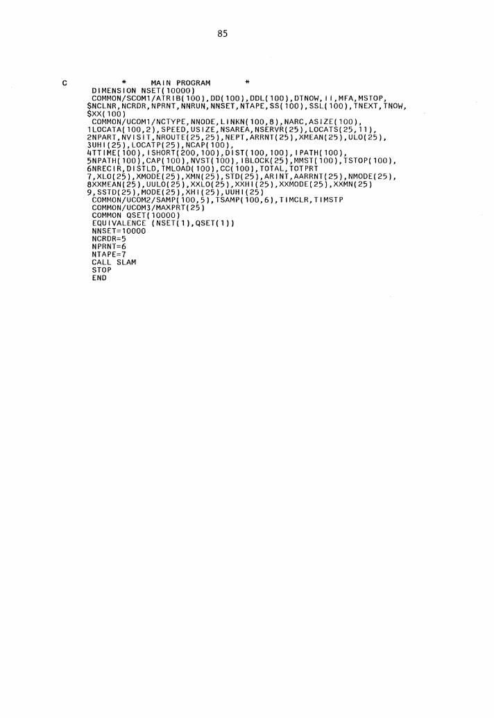
85
C * MAIN PROGRAM * DIMENSION NSET(10000) COMMON/SCOM1/ATRIB(100),DD(100),DDL(100),DTNOW, I l,MFA,MSTOP,
$NCLNR,NCRDR,NPRNT,NNRUN,NNSET,NTAPE,SS(100),SSL(100),TNEXT,TNOW, $XX(100)
COMMON/UCOM1/NCTYPE,NNODE,LINKN(100,8),NARC,ASIZE(100), 1LOCATA(100,2),SPEED,USIZE,NSAREA,NSERVR(25),LOCATS(25,11), 2NPART,NVISIT,NROUTE(25,25),NEPT,ARRNT(25),XMEAN(25),UL0(25), 3UHl(25),LOCATP(25),NCAP(100), 4TT I ME( 100), I SHORT( 200, 100), DI ST( 100, 100), I PATH( 100), 5NPATH( 100), CAP( 100), NVST( 100), I BLOCK( 25), MMST( 100), TSTOP( 100). 6NRECIR,DISTLD, TMLOAD(100),CC(100), TOTAL,TOTPRT 7,XL0(25),XMODE(25),XMN(25),STD(25),ARINT,AARRNT(25),NMODE(25), 8XXMEAN(25),UUL0(25),XXL0(25),XXHl(25),XXMODE(25),XXMN(25) 9,SSTD(25),MODE(25),XH1(25),UUHl(25)
COMMON/UCOM2/SAMP(100,5), TSAMP(100,6),TIMCLR,TIMSTP COMMON/UCOM3/MAXPRT(25) COMMON QSET(10000) EQUIVALENCE (NSET(1),QSET(1)) NNSET=10000 NCRDR=5 NPRNT=6 NTAPE=7 CALL SLAM STOP END
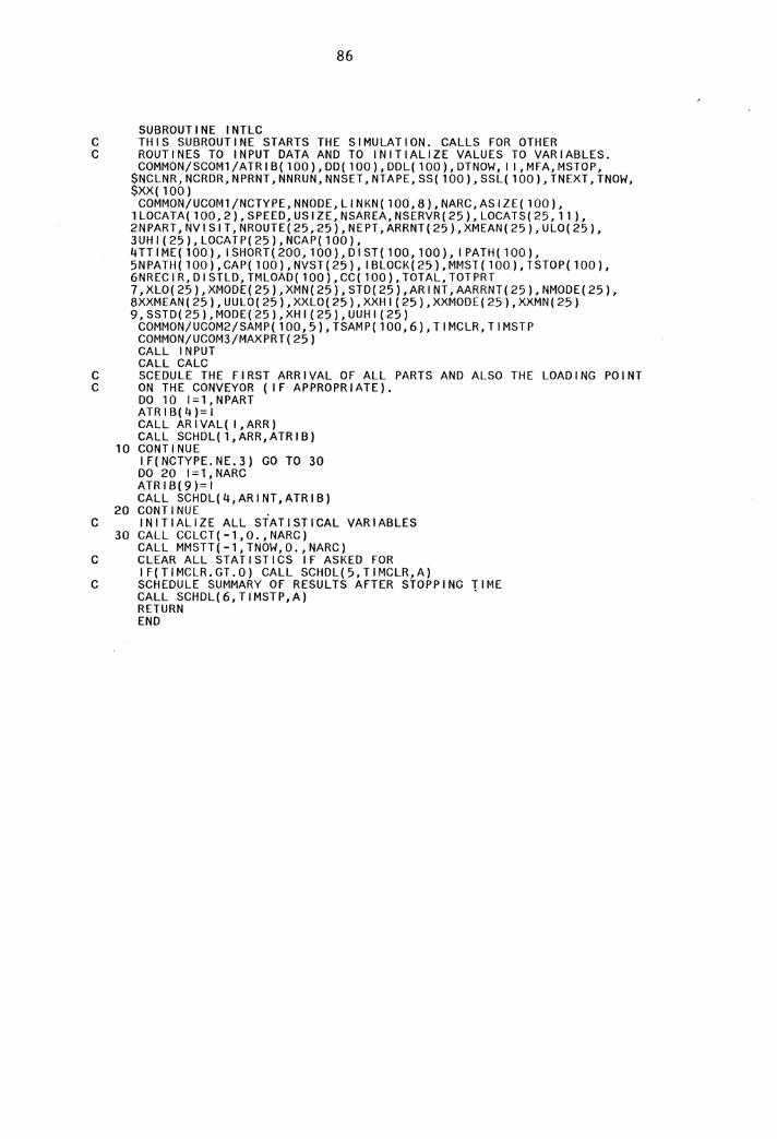
86
SUBROUTINE INTLC C THIS SUBROUTINE STARTS THE SIMULATION. CALLS FOR OTHER C ROUTINES TO INPUT DATA AND TO INITIALIZE VALUES TO VARIABLES.
COMMON/SCOM1/ATRIB(100),DD(100),DDL(100),DTNOW, I l,MFA,MSTOP, $NCLNR,NCRDR,NPRNT,NNRUN,NNSET,NTAPE,SS(100),SSL(100),TNEXT,TNOW, $XX(100)
COMMON/UCOM1/NCTYPE,NNODE,LINKN(100,8),NARC,ASIZE(100), 1LOCATA(100,2),SPEED,USIZE,NSAREA,NSERVR(25),LOCATS(25,11), 2NPART,NVISIT,NROUTE(25,25),NEPT,ARRNT(25),XMEAN(25),UL0(25), 3UHl(25),LOCATP(25),NCAP(100), 4TTIME(100), ISHORT(200,100),DIST(100,100), IPATH(100), 5NPATH(100),CAP(100),NVST(25), IBLOCK(25),MMST(100),TSTOP(100), 6NRECIR,DISTLD,TMLOAD(100),CC(100),TOTAL,TOTPRT 7,XL0(25),XMODE(25),XMN(25),STD(25),ARINT,AARRNT(25),NMODE(25), 8XXMEAN(25),UUL0(25),XXL0(25),XXHl(25),XXMODE(25),XXMN(25) 9,SSTD(25),MODE(25),XH1(25),UUHl(25)
COMMON/UCOM2/SAMP(100,5),TSAMP(100,6),TIMCLR,TIMSTP COMMON/UCOM3/MAXPRT(25) CALL INPUT CALL CALC
C SCEDULE THE FIRST ARRIVAL OF ALL PARTS AND ALSO THE LOADING POINT C ON THE CONVEYOR (IF APPROPRIATE).
DO 10 1=1,NPART ATRIB(4)=1 CALL ARIVAL( l,ARR) CALL SCHDL(l,ARR,ATRIB)
10 CONTINUE IF(NCTYPE.NE.3) GO TO 30 DO 20 1=1,NARC ATRIB(9)=1 CALL SCHDL(4,ARINT,ATRIB)
20 CONTINUE . C INITIALIZE ALL STATISTICAL VARIABLES
30 CALL CCLCT(-1,0.,NARC) CALL MMSTT(-1,TNOW,O.,NARC)
C CLEAR ALL STATISTICS IF ASKED FOR IF(TIMCLR.GT.O) CALL SCHDL(5,TIMCLR,A)
C SCHEDULE SUMMARY OF RESULTS AFTER STOPPING TIME CALL SCHDL(6,TIMSTP,A) RETURN END
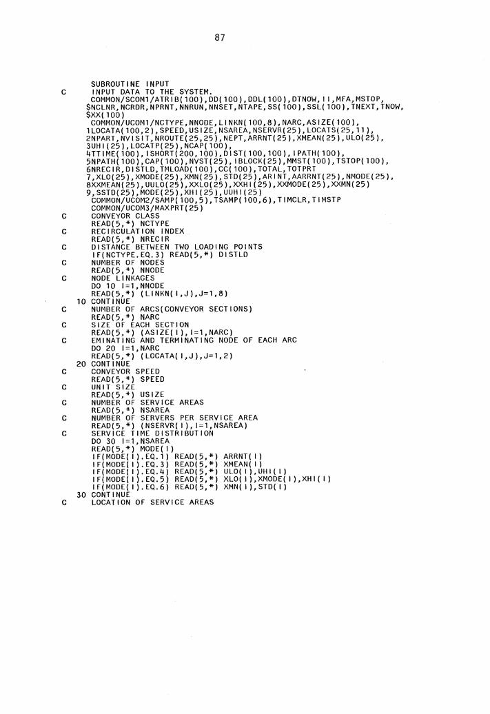
87
SUBROUTINE INPUT C INPUT DATA TO THE SYSTEM.
COMMON/SCOM1/ATRIB(100),DD(100),DDL(100),DTNOW, I l,MFA,MSTOP, $NCLNR,NCRDR,NPRNT,NNRUN,NNSET,NTAPE,SS(100),SSL(100), TNEXT, TNOW, $XX(100)
COMMON/UCOM1/NCTYPE,NNODE,LINKN(100,8),NARC,ASIZE(100), 1LOCATA(100,2),SPEED,USIZE,NSAREA,NSERVR(25),LOCATS(25,11), 2NPART,NVISIT,NROUTE(25,25),NEPT,ARRNT(25),XMEAN(25),UL0(25), 3UHl(25),LOCATP(25),NCAP(100), 4TT IME( 100), I SHORT( 200, 100), DI ST( 100, 100), I PATH( 100), 5NPATH(100),CAP(100),NVST(25), IBLOCK(25),MMST(100),TSTOP(100), 6NRECIR,DISTLD,TMLOAD(100),CC(100),TOTAL,TOTPRT 7,XL0(25),XMODE(25),XMN(25),STD(25),ARINT,AARRNT(25),NMODE(25), 8XXMEAN(25),UUL0(25),XXL0(25),XXHl(25),XXMODE(25),XXMN(25) 9,SSTD(25),MODE(25),XHl(25),UUHl(25)
COMMON/UCOM2/SAMP(100,5),TSAMP(100,6),TIMCLR,TIMSTP COMMON/UCOM3/MAXPRT(25)
C CONVEYOR CLASS READ(5,*) NCTYPE
C RECIRCULATION INDEX READ(5,*) NRECIR
C DISTANCE BETWEEN TWO LOADING POINTS IF(NCTYPE.EQ.3) READ(5,*) DISTLD
C NUMBER OF NODES READ(5,*) NNODE
C NODE LINKAGES DO 10 1=1,NNODE READ(5,*) (LINKN( l,J),J=1,8)
10 CONTINUE C NUMBER OF ARCS(CONVEYOR SECTIONS)
READ(5,*) NARC C SIZE OF EACH SECTION
READ(5,*) (ASIZE( I), 1=1,NARC) C EMINATING AND TERMINATING NODE OF EACH ARC
DO 20 1=1,NARC READ(5,*) (LOCATA( l,J),J=1,2)
20 CONTINUE C CONVEYOR SPEED
READ(5,*) SPEED C UNIT SIZE
READ(5,*) USIZE C NUMBER OF SERVICE AREAS
READ(5,*) NSAREA C NUMBER OF SERVERS PER SERVICE AREA
READ(5,*) (NSERVR( I), 1=1,NSAREA) C SERVICE TIME DISTRIBUTION
DO 30 1=1,NSAREA READ(5,*) MODE( I) IF(MODE(l).EQ.1) READ(5,*) ARRNT(I) IF(MODE( l).EQ.3) READ(5,*) XMEAN( I) IF(MODE(l).EQ.4) READ(5,*) ULO(l),UHl(I) IF( MODE( I ).EQ.5) READ(5,*) XLO( I ),XMODE( I ),XHI( I) IF(MODE(l).EQ.6) READ(5,*) XMN(l),STD(I)
30 CONTINUE C LOCATION OF SERVICE AREAS
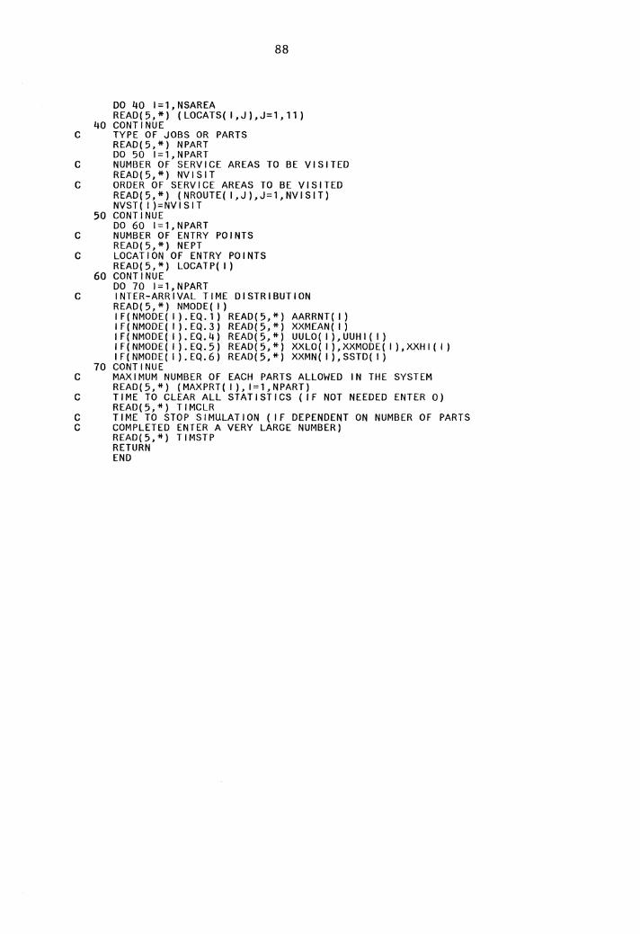
88
DO 40 1=1,NSAREA READ(5,*) (LOCATS( l,J),J=l,11)
40 CONTINUE C TYPE OF JOBS OR PARTS
READ(5,*) NPART DO 50 1=1,NPART
C NUMBER OF SERVICE AREAS TO BE VISITED READ(5,*) NVISIT
C ORDER OF SERVICE AREAS TO BE VISITED READ(5,*) (NROUTE( l,J),J=1,NVISIT) NVST( I )=NVISIT
50 CONTINUE DO 60 1=1,NPART
C NUMBER OF ENTRY POINTS READ(5,*) NEPT
C LOCATION OF ENTRY POINTS READ(5,*) LOCATP( I)
60 CONTINUE DO 70 1=1,NPART
C INTER-ARRIVAL TIME DISTRIBUTION READ(5,*) NMODE( I) IF(NMODE(l).EQ.1) READ(5,*) AARRNT(I) IF( NMODE( I). EQ. 3) READ( 5, *) XXMEAN( I) IF(NMODE( I ).EQ.4) READ(5,*) UULO( I ),UUHI( I) IF( NMODE( I). EQ. 5) READ( 5, *) XXLO( I ),XXMODE( I) ,XXH I (I) IF(NMODE( I ).EQ.6) READ(5,*) XXMN( I ),SSTD( I)
70 CONTINUE C MAXIMUM NUMBER OF EACH PARTS ALLOWED IN THE SYSTEM
READ(5,*) (MAXPRT( I), 1=1,NPART) C TIME TO CLEAR ALL STATISTICS (IF NOT NEEDED ENTER 0)
READ(5,*) TIMCLR C TIME TO STOP SIMULATION (IF DEPENDENT ON NUMBER OF PARTS C COMPLETED ENTER A VERY LARGE NUMBER)
READ(5,*) TIMSTP RETURN END
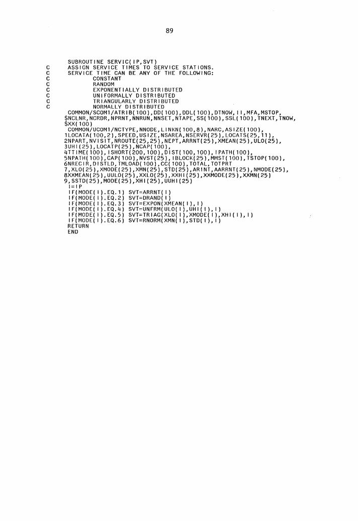
89
SUBROUTINE SERVIC( IP,SVT) C ASSIGN SERVICE TIMES TO SERVICE STATIONS. C SERVICE TIME CAN BE ANY OF THE FOLLOWING: C CONSTANT C RANDOM C EXPONENTIALLY DISTRIBUTED C UNIFORMALLY DISTRIBUTED C TRIANGULARLY DISTRIBUTED C NORMALLY DISTRIBUTED
COMMON/SCOM1/ATRIB(100),DD(100),DDL(100),DTNOW, I l,MFA,MSTOP, $NCLNR,NCRDR,NPRNT,NNRUN,NNSET,NTAPE,SS(100),SSL(100),TNEXT,TNOW, $XX(100)
COMMON/UCOM1/NCTYPE,NNODE,LINKN(100,8),NARC,ASIZE(100), 1LOCATA(100,2),SPEED,USIZE,NSAREA,NSERVR(25),LOCATS(25,11), 2NPART,NVISIT,NROUTE(25,25),NEPT,ARRNT(25),XMEAN(25),UL0(25), 3UHl(25),LOCATP(25),NCAP(100), 4TT I ME( 100), I SHORT( 200, 100), DI ST( 100, 100), I PATH( 100), 5N PA TH ( 100), CAP ( 100), NVST ( 25), I BLOCK( 25), MMST ( 100), TSTOP( 100), 6NRECIR,DISTLD,TMLOAD(100),CC(100), TOTAL,TOTPRT 7,XL0(25),XMODE(25),XMN(25),STD(25),ARINT,AARRNT(25),NMODE(25), 8XXMEAN(25),UUL0(25),XXL0(25),XXHl(25),XXMODE(25),XXMN(25) 9,SSTD(25),MODE(25),XHl(25),UUHl(25)
l=IP IF(MODE(l).EQ.1) SVT=ARRNT(I) IF(MODE(l).EQ.2) SVT=DRAND(I) IF( MODE( I ).EQ.3) SVT=EXPON(XMEAN( I), I) IF( MODE( I ).EQ.4) SVT=UNFRM(ULO( I ),UHi( I), I) I F(MODE( I). EQ.5) SVT=TRIAG(XLO( I ),XMODE( I ),XH I (I), I) IF( MODE( I ).EQ.6) SVT=RNORM(XMN( I ),STD( I), I) RETURN END
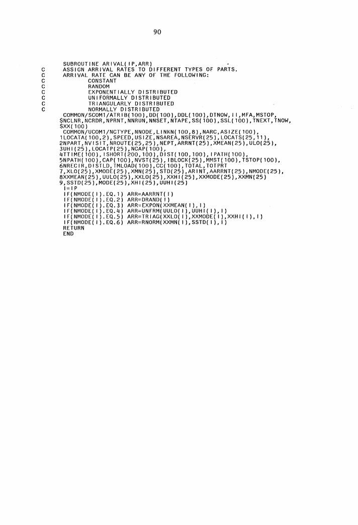
90
SUBROUTINE ARIVAL( IP,ARR) C ASSIGN ARRIVAL RATES TO DIFFERENT TYPES OF PARTS. C ARRIVAL RATE CAN BE ANY OF THE FOLLOWING: C CONSTANT C RANDOM C EXPONENTIALLY DISTRIBUTED C UNIFORMALLY DISTRIBUTED C TRIANGULARLY DISTRIBUTED C NORMALLY DISTRIBUTED
COMMON/SCOM1/ATRI B( 100), DD( 100), DDL( 100), DTNOW, I I, MFA, MSTOP, $NCLNR,NCRDR,NPRNT,NNRUN,NNSET,NTAPE,SS(100),SSL(100),TNEXT,TNOW, $XX(100)
COMMON/UCOM1/NCTYPE,NNODE,LINKN(100,8),NARC,ASIZE(100), 1LOCATA(100,2),SPEED,USIZE,NSAREA,NSERVR(25),LOCATS(25,11), 2NPART,NVISIT,NROUTE(25,25),NEPT,ARRNT(25),XMEAN(25),UL0(25), 3UHl(25),LOCATP(25),NCAP(100), 4TTIME( 100), ISHORT(200, 100), DIST( 100, 100), I PATH( 100), 5NPATH( 100), CAP( 100), NVST(25), I BLOCK( 25), MMST( 100 ), TSTOP( 100), 6NRECIR,DISTLD,TMLOAD(100),CC(100),TOTAL,TOTPRT 7, XLO( 25), XMODE( 25), XMN( 25), STD( 25) ,AR I NT, AARRNT( 25), NMODE( 25), 8XXMEAN(25),UUL0(25),XXL0(25),XXH1(25),XXMODE(25),XXMN(25) 9,SSTD(25),MODE(25),XHl(25),UUHl(25)
l=IP IF(NMODE( I ).EQ.1) ARR=AARRNT( I) IF(NMODE( l).EQ.2) ARR=DRAND( I) IF(NMODE( I ).EQ.3) ARR=EXPON(XXMEAN( I), I) IF( NMODE( I). EQ. 4) ARR=UNFRM( UULO( I), UUH I ( I), I) IF( NMODE( I). EQ. 5) ARR= TR I AG( XXLO( I ),XXMODE( I) ,XXH I ( I), I) IF( NMODE( I). EQ. 6) ARR=RNORM(XXMN( I), SSTD( I), I) RETURN END
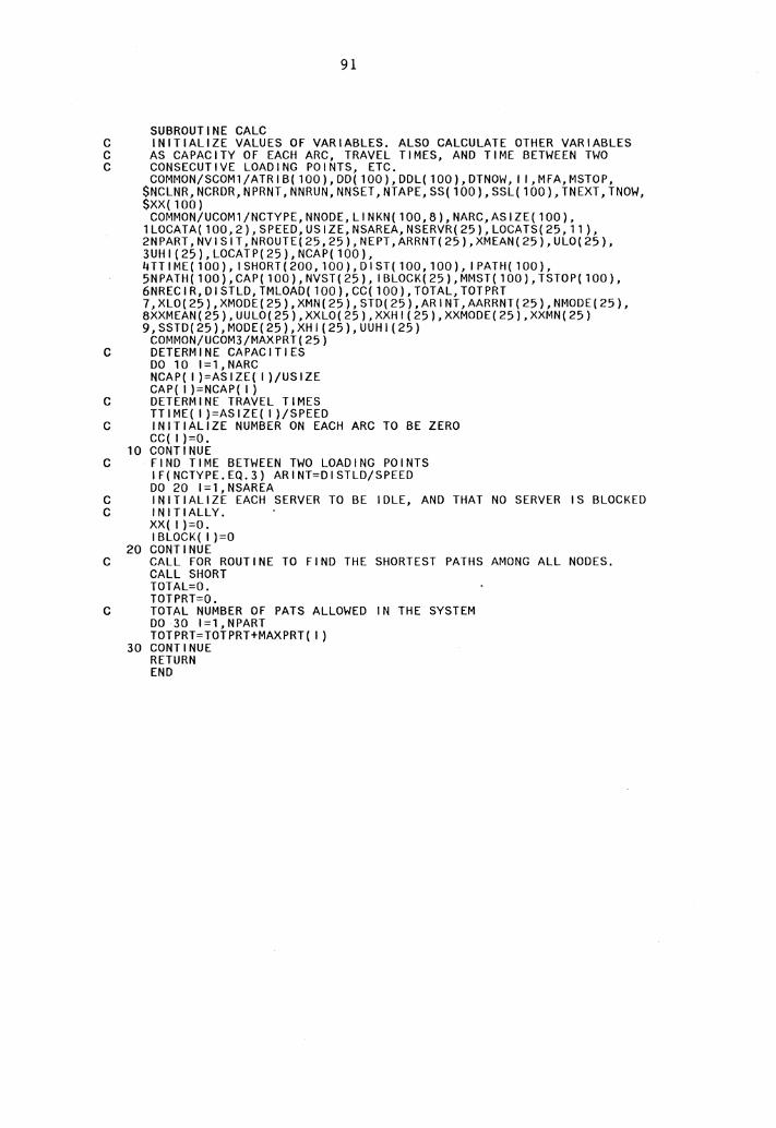
91
SUBROUTINE CALC C INITIALIZE VALUES OF VARIABLES. ALSO CALCULATE OTHER VARIABLES C AS CAPACITY OF EACH ARC, TRAVEL TIMES, AND TIME BETWEEN TWO C CONSECUTIVE LOADING POINTS, ETC.
COMMON/SCOMl/ATRIB(lOO),DD(lOO),DDL(lOO),DTNOW, I l,MFA,MSTOP, $NCLNR,NCRDR,NPRNT,NNRUN,NNSET,NTAPE,SS(100),SSL(100),TNEXT,TNOW, $XX(100)
COMMON/UCOMl/NCTYPE,NNODE,LINKN(l00,8),NARC,ASIZE(lOO), 1LOCATA(100,2),SPEED,USIZE,NSAREA,NSERVR(25),LOCATS(25,11), 2NPART,NVISIT,NROUTE(25,25),NEPT,ARRNT(25),XMEAN(25),UL0(25), 3UHl(25),LOCATP(25),NCAP(100), 4TT IME( 100) I I SHORT( 200, 100)' DIST( 100, 100) I I PATH( 100)' 5NPATH( 100),CAP( 100),NVST(25), IBLOCK(25),MMST( 100), TSTOP( 100), 6NRECIR,DISTLD, TMLOAD(lOO),CC(lOO),TOTAL,TOTPRT 7,XL0(25),XMODE(25),XMN(25),STD(25),ARINT,AARRNT(25),NMODE(25), 8XXMEAN(25),UUL0(25),XXL0(25),XXHl(25),XXMODE(25),XXMN(25) 9,SSTD(25),MODE(25),XHl(25),UUHl(25)
COMMON/UCOM3/MAXPRT(25) C DETERMINE CAPACITIES
DO 10 1=1, NARC NCAP( I )=ASIZE( I )/USIZE CAP( I )=NCAP( I)
C DETERMINE TRAVEL TIMES TTIME( I )=ASIZE( I )/SPEED
C INITIALIZE NUMBER ON EACH ARC TO BE ZERO CC(l)=O.
10 CONTINUE C FIND TIME BETWEEN TWO LOADING POINTS
IF(NCTYPE.EQ.3) ARINT=DISTLD/SPEED DO 20 1=1,NSAREA
C INITIALIZE EACH SERVER TO BE IDLE, AND THAT NO SERVER IS BLOCKED C INITIALLY.
XX(l)=O. I BLOCK( I )=O
20 CONTINUE C CALL FOR ROUTINE TO FIND THE SHORTEST PATHS AMONG ALL NODES.
CALL SHORT TOTAL=O. TOTPRT=O.
C TOTAL NUMBER OF PATS ALLOWED IN THE SYSTEM DO 30 1=1,NPART TOTPRT=TOTPRT+MAXPRT( I )
30 CONTINUE RETURN END
92
SUBROUTINE SHORT C DETERMINE THE SHORTEST PATHS AMONG ALL NODES.
COMMON/SCOMl/ATRIB(lOO),DD(lOO),DDL(lOO),DTNOW, I l,MFA,MSTOP, $NCLNR,NCRDR,NPRNT,NNRUN,NNSET,NTAPE,SS(100),SSL(l00),TNEXT, TNOW, $XX(100)
COMMON/UCOMl/NCTYPE,NNODE,LINKN(l00,8),NARC,ASIZE(lOO), 1LOCATA(100,2),SPEED,USIZE,NSAREA,NSERVR(25),LOCATS(25,11), 2NPART,NVISIT,NROUTE(25,25),NEPT,ARRNT(25),XMEAN(25),UL0(25), 3UHl(25),LOCATP(25),NCAP(100), 4TT I ME( 100), I SHORT( 200, 100), DI ST( 100, 100), I PATH( 100), 5NPATH( 100), CAP( 100), NVST( 25), I BLOCK( 25), MMST( 100), TSTOP( 100), 6NRECIR,DISTLD,TMLOAD(100),CC(100),TOTAL,TOTPRT 7,XL0(25),XMODE(25),XMN(25),STD(25),ARINT,AARRNT(25),NMODE(25), 8XXMEAN(25),UUL0(25),XXL0(25),XXHl(25),XXMODE(25),XXMN(25) 9,SSTD(25),MODE(25),XH1(25),UUHl(25)
DIMENSION INCID(l00,3),NWORK(l00,2),TT(lOO),WW(lOO), *PP(lOO),PL(lOO),DWORK(lOO)
INTEGER TT,WW,PP DATA WW/100*0/,TT/100*0/,PP/100*0/,PL/100*0./,NWORK/200*0/,DWORK/l
100*0./ MNODE=2*NNODE DO 20 1=1,NNODE DO 10 J=6, 8 K=J-5 INCID( l,K)=LINKN( l,J)
10 CONTINUE IF( INCID( I, 1) .GT.O)WW( I )=WW( I )+1 IF( INCID( 1,2).GT.O)WW( I )=WW( I )+1 IF( INCID( 1,3).GT.O)WW( I )=WW( I )+1
20 CONTINUE C FIND THE SHORTEST PATH TO ALL THE NODES FROM NODE K
ITOTAL=3*NNODE · K=l
C REMOVE NODE K FROM MATRIX WW M=l WW(K)=O TT(M)=K PP(M)=O PL(M)=O
C FIND NODES ADJACENT TO THE NODES THAT CURRENTLY HAS PERMANENT C LABEL THAT ARE IN MATRIX WW
25 IC=TT(M) DO 30 MX=l,3 NN=INCID( IC,MX)
C CHECK IF NODE NN EXISTS IF(NN.EQ.O)GO TO 30
C CALCULATE DISTANCE,SET POINTER C IC=PRECEEDING NODE; NN=SUCCEEDING NODE.
I POINT=3*( IC-1) + MX NWORK( IPOINT, l)=IC NWORK( IPOINT,2)=NN
C DISTANCE CALCULATION CALL FINDD( IC,NN) DWORK( I POINT)=DIST( IC,NN)+PL(M)
30 CONTINUE
93
C PICK THE NODE CLOSEST FROM NODE K IF(M.GE.MNODE)GO TO 60 AMIN=lOOOOOOOO. DO 40 KF=l, I TOTAL IF(DWORK(KF).LE.AMIN.AND.DWORK(KF).GT.O. )ISUCC=NWORK(KF,2) IF(DWORK(KF).LE.AMIN.AND.DWORK(KF).GT.O. )IPREC=NWORK(KF,1) IF(DWORK(KF).LE.AMIN.AND.DWORK(KF).GT.O. )AMIN=DWORK(KF)
40 CONTINUE C ASSIGN PERMANENT LABEL TO THE NODE NEAREST FROM K FROM THE SET OF NODES C WHOSE DISTANCES ARE COMPUTED AND ARE IN MATRIX WW
M=M+l TT(M)=ISUCC PP(M)=IPREC PL(M)=AMIN
C DELETE ALL OTHER PATHS LEADING INTO NODE 'ISUCC' THAT ARE NOT THE C SHORTEST PATHS FROM NODE K
WW( ISUCC)=O DO 50 KF=l, I TOTAL IF(NWORK(KF,2).NE. ISUCC)GO TO 50 NWORK(KF,1)=0 NWORK(KF,2)=0 DWORK(KF)=O.
50 CONTINUE C NOW FIND THE NODES INCIDENT FROM 'ISUCC' THAT ARE IN MATRIX WW
GO TO 25 C MINIMUM PATHS HAVE BEEN FOUND FOR ALL NODES FROM NODE K C PLACE PATH AND DISTANCE IN THE SHORTEST PATH MATRIX
60 LT=( 2*K) - 1 LP=2*K DO 70 IX=l,M I SHORT( LT, IX)=TT( IX) LINE=TT( IX) TT( IX)=O I SHORT( LP, IX)=PP( IX) PP( IX)=O PL( IX)=O.
70 WW( IX)=IX C SHORTEST PATH FROM ALL NODES TO ALL OTHER NODES FOUND?
K=K+l IF(K.GT.NNODE)GO TO 80
C NO. SHORTEST PATH NOT YET FOUND FOR ALL NODES. C FIND THE SHORTEST PATH FROM NODE K. RESET M TO
M=l TT(M)=K WW(K)=O GO TO 25
C ALL SHORTEST PATHS ARE FOUND. PRINT OUT THE STRING OF TRACEABLE PATHS. 80 RETURN
END
94
SUBROUTINE FINDD( IC,NN) C FIND THE DISTANT BETWEEN TWO ADJACENT NODES.
COMMON/SCOM1/ATRIB(100),DD(100),DDL(100),DTNOW, I l,MFA,MSTOP, $NCLNR,NCRDR,NPRNT,NNRUN,NNSET,NTAPE,SS(100),SSL(100),TNEXT,TNOW, $XX(100) COMMON/UCOM1/NCTYPE,NNODE,LINKN(100,8),NARC,ASIZE(100),
1LOCATA(100,2),SPEED,USIZE,NSAREA,NSERVR(25),LOCATS(25,11), 2NPART,NVISIT,NROUTE(25,25),NEPT,ARRNT(25),XMEAN(25),UL0(25), 3UHl(25),LOCATP(25),NCAP(100), 4TT IME( 100), I SHORT( 200, 100), DI ST( 100, 100), I PATH( 100), 5NPATH( 100),CAP( 100),NVST(25), IBLOCK(25),MMST( 100), TSTOP( 100), 6NRECIR,DISTLD, TMLOAD(100),CC(100),TOTAL,TOTPRT 7,XL0(25),XMODE(25),XMN(25),STD(25),ARINT,AARRNT(25),NMODE(25), 8XXMEAN(25),UUL0(25),XXL0(25),XXHl(25),XXMODE(25),XXMN(25) 9,SSTD(25),MODE(25),XHl(25),UUHl(25)
DO 10 1=1,NARC C FIRST FIND OUT THE ARC NUMBER BETWEEN THE TWO NODES
NSUC=LOCATA( I, 1) I F(NSUC.NE. IC) GO TO 10 IF(LOCATA(l,2).NE.NN) GO TO 10
C ARC NUMBER FOUND. NRARC=I GO TO 15
10 CONT I NUE C LOOK FOR THE DISTANCE IN THE ARC SIZE MATRIX
15 DIST( IC,NN)=ASIZE(NRARC) RETURN END
95
SUBROUTINE FINDA( IC,NN,NNARC) C FIND OUT THE ARC NUMBER WHICH LINKS NODES IC AND NN
COMMON/SCOMl/ATRIB(lOO),DD(lOO),DDL(lOO),DTNOW, I l,MFA,MSTOP, $NCLNR,NCRDR,NPRNT,NNRUN,NNSET,NTAPE,SS(l00),SSL(l00), TNEXT,TNOW, $XX(100)
COMMON/UCOMl/NCTYPE,NNODE,LINKN(l00,8),NARC,ASIZE(lOO), lLOCATA(l00,2),SPEED,USIZE,NSAREA,NSERVR(25),LOCATS(25,ll), 2NPART,NVISIT,NROUTE(25,25),NEPT,ARRNT(25),XMEAN(25),UL0(25), 3UHl(25),LOCATP(25),NCAP(l00), 4TT IME( 100), I SHORT( 200, 100), DI ST( 100, 100), I PATH( 100), 5NPATH( 100), CAP( 100), NVST( 25), I BLOCK( 25), MMST( 100), TSTOP( 100), 6NRECIR,DISTLD, TMLOAD(100),CC(100),TOTAL,TOTPRT 7,XL0(25),XMODE(25),XMN(25),STD(25),ARINT,AARRNT(25),NMODE(25), 8XXMEAN(25),UUL0(25),XXL0(25),XXHl(25),XXMODE(25),XXMN(25) 9,SSTD(25),MODE(25),XH1(25),UUHl(25)
C SEE IF THE EMINATING NODE CORRESPONDS TO IC DO 10 1=1,NARC NSUC=LOCATA( I, 1) IF(NSUC.NE. IC) GO TO 10
C CHECK FOR THE TERMINATING NODE IF(LOCATA( 1,2).NE.NN) GO TO 10
C ARC NUMBER IS I NNARC=I GO TO 15
10 CONTINUE 15 RETURN
END
96
SUBROUTINE FINDL(NODFR) C FIND THE LAST NODE A PART HAS VISITED
COMMON/SCOM1/ATRIB(100),DD(100),DDL(100),DTNOW, I l,MFA,MSTOP, $NCLNR,NCRDR,NPRNT,NNRUN,NNSET,NTAPE,SS(100),SSL(100),TNEXT,TNOW, $XX(100) COMMON/UCOM1/NCTYPE,NNODE,LINKN(100,8),NARC,ASIZE(100),
1LOCATA(100,2),SPEED,USIZE,NSAREA,NSERVR(25),LOCATS(25,11), 2NPART,NVISIT,NROUTE(25,25),NEPT,ARRNT(25),XMEAN(25),UL0(25), 3UHl(25),LOCATP(25),NCAP(100), 4TT I ME( 100), I SHORT( 200, 100), DI ST( 100, 100), I PATH( 100), 5NPATH( 100), CAP( 100), NVST( 25), I BLOCK(25), MMST( 100), TSTOP( 100), 6NRECIR,DISTLD,TMLOAD(100),CC(100),TOTAL,TOTPRT 7,XL0(25),XMODE(25),XMN(25),STD(25),ARINT,AARRNT(25),NMODE(25), 8XXMEAN(25),UUL0(25),XXL0(25),XXH1(25),XXMODE(25),XXMN(25) 9,SSTD(25),MODE(25),XH1(25),UUHl(25)
C FIND THE LAST ARC VISITED AND THE CURRENT NODE LASTAR=ATRIB(9)+0.5 LASTND=ATRIB(11)+0.5
C FIND THE NODE FROM WHICH THE LAST ARC VISITED EMINATES C AND LEADS TO THE CURRENT NODE
DO 10 1=1,NARC IF( l.NE.LASTAR) GO TO 10 IF(LOCATA( 1,2).EQ.LASTND) GO TO 20
10 CONTINUE CALL ERROR RETURN
C REQUIREQ NODE FOUND 20NODFR=LOCATA(1,1)
RETURN END
97
SUBROUTINE FINDS(NODAT,NSTN,EX) C DETERMINE IF A NODE (NODAT) IS A SERVICE STATION (NSTN)?
COMMON/SCOM1/ATRIB(100),DD(100),DDL(100),DTNOW, I l,MFA,MSTOP, $NCLNR,NCRDR,NPRNT,NNRUN,NNSET,NTAPE,SS(100),SSL(100),TNEXT,TNOW, $XX( 100) .
COMMON/UCOM1/NCTYPE,NNODE,LINKN(100,8),NARC,ASIZE(100), 1LOCATA(100,2),SPEED,USIZE,NSAREA,NSERVR(25),LOCATS(25,11), 2NPART,NVISIT,NROUTE(25,25),NEPT,ARRNT(25),XMEAN(25),UL0(25), 3UHl(25),LOCATP(25),NCAP(100), 4TT IME( 100), I SHORT( 200, 100) I DI ST( 100, 100) I I PATH( 100) I 5NPATH(100),CAP(100),NVST(25), IBLOCK(25),MMST(100),TSTOP(100), 6NRECIR,DISTLD,TMLOAD(100),CC(100),TOTAL,TOTPRT 7,XL0(25),XMODE(25),XMN(25),STD(25),ARINT,AARRNT(25),NMODE(25), 8XXMEAN(25),UUL0(25),XXL0(25),XXHl(25),XXMODE(25),XXMN(25) 9,SSTD(25),MODE(25),XHl(25),UUHl(25)
DO 20 1=1,NSAREA K=1 J=LOCATS( I, 1) DO 10 JJ=1,J K=K+1 IF(LOCATS( l,K).EQ.NODAT) GO TO 30
C NOT A SERVICE STATION EX=O.
10 CONTINUE 20 CONTINUE
RETURN C SERVICE STATION
30 EX=1. NSTN=I RETURN END
98
SUBROUTINE FINDS2(NTHIS,NEXT) C DETERMINE THE NODE NUMBERS FOR NODES WHICH CORRESPOND TO C THE SERVICE STATIONS (NTHIS,NEXT).
COMMON/SCOM1/ATRIB(100),DD(100),DDL(100),DTNOW, I l,MFA,MSTOP, $NCLNR,NCRDR,NPRNT,NNRUN,NNSET,NTAPE,SS(100),SSL(100),TNEXT,TNOW, $XX(100)
COMMON/UCOM1/NCTYPE,NNODE,LINKN(100,8),NARC,ASIZE(100), 1LOCATA(100,2),SPEED,USIZE,NSAREA,NSERVR(25),LOCATS(25,11), 2NPART,NVISIT,NROUTE(25,25),NEPT,ARRNT(25),XMEAN(25),UL0(25), 3UHl(25),LOCATP(25),NCAP(100), 4TT I ME( 100), I SHORT( 200, 100), DI ST( 100, 100), I PATH( 100), 5NPATH( 100), CAP( 100), NVST( 25), I BLOCK( 25) ,MMST( 100), TSTOP( 100), 6NRECIR,DISTLD,TMLOAD(100),CC(100),TOTAL,TOTPRT 7,XL0(25),XMODE(25),XMN(25),STD(25),ARINT,AARRNT(25),NMODE(25), 8XXMEAN(25),UUL0(25),XXL0(25),XXHl(25),XXMODE(25),XXMN(25) 9,SSTD(25),MODE(25),XH1(25),UUHl(25) J=LOCATS(NTHIS,1) IF(J.EQ.1) GO TO 20
10 CALL ERROR RETURN
20 NTHIS=LOCATS(NTHIS,2) K=LOCATS(NEXT,1) IF(K.NE.1) GO TO 10 NEXT=LOCATS(NEXT,2) RETURN END
99
SUBROUTINE EVENT( I) C DIRECTS TO THE PROPER EVENT. SIX EVENTS ARE C ARRIVAL TO CONVEYOR C END OF CONVEYOR C END OF SERVICE C ARRIVAL OF A LOADING POINT (ONLY FOR CLASS 3 TYPE CONVEYORS). C CLEAR STATISTICS C PRINT SUMMARY
GO TO (1,2,3,4,5,6), I CALL ARRIV( I) RETURN
2 CALL CONVR( I) RETURN
3 CALL ENDSV( I ) RETURN
4 CALL LOAD( I) RETURN
5 CALL CLRST RETURN
6 CALL SMMRY RETURN END
100
SUBROUTINE ARRIV( I) C EVENT 1: ARRIVAL TO A CONVEYOR. DIRECT TO THE PROPER ROUTINE
COMMON/SCOM1/ATRIB(100),DD(100),DDL(100),DTNOW, I l,MFA,MSTOP, $NCLNR,NCRDR,NPRNT,NNRUN,NNSET,NTAPE,SS(100),SSL(100),TNEXT,TNOW, $XX(100)
COMMON/UCOM1/NCTYPE,NNODE,LINKN(100,8),NARC,ASIZE(100), 1LOCATA(100,2),SPEED,USIZE,NSAREA,NSERVR(25),LOCATS(25,11), 2NPART,NVISIT,NROUTE(25,25),NEPT,ARRNT(25),XMEAN(25),UL0(25), 3UHl(25),LOCATP(25),NCAP(100), 4TTIME(100), ISHORT(200,100),DIST(100,100), IPATH(100), 5NPATH(100),CAP(100),NVST(25), IBLOCK(25),MMST(100), TSTOP(100), 6NRECIR,DISTLD,TMLOAD(100),CC(100),TOTAL,TOTPRT 7,XL0(25),XMODE(25),XMN(25),STD(25),ARINT,AARRNT(25),NMODE(25), 8XXMEAN(25),UUL0(25),XXL0(25),XXHl(25),XXMODE(25),XXMN(25) 9,SSTD(25),MODE(25),XHl(25),UUHl(25)
GO TO (1,2,3),NCTYPE C CONVEYOR CLASS 1 C IS THIS AN OLD PART ?
IF(ATRIB(7).GT.O.) CALL OLD1 C IS THIS A NEW PART ?
IF(ATRIB(7).EQ.O.) CALL NEW1 RETURN
C CONVEYOR CLASS 2 C IS THIS AN OLD PART ?
2 IF(ATRIB(7).GT.O.) CALL OLD2 C IS THIS A NEW PART ?
IF(ATRIB(7).EQ.O.) CALL NEW2 RETURN
C CONVEYOR CLASS 3 C IS THIS AN OLD PART ?
3 IF(ATRIB(7).GT.O.) CALL OLD3 C IS THIS A NEW PART ?
IF(ATRIB(7).EQ.O.) CALL NEW3 RETURN END
101
SUBROUTINE CONVR( I) C EVENT 2: END OF A CONVEYOR, DIRECT TO THE PROPER ROUTINE.
COMMON/SCOM1/ATRIB(100),DD(100),DDL(100),DTNOW, I l,MFA,MSTOP, $NCLNR,NCRDR,NPRNT,NNRUN,NNSET,NTAPE,SS(100),SSL(100),TNEXT,TNOW, $XX(100) .
COMMON/UCOM1/NCTYPE,NNODE,LINKN(100,8),NARC,ASIZE(100), 1LOCATA(100,2),SPEED,USIZE,NSAREA,NSERVR(25),LOCATS(25,11), 2NPART,NVISIT,NROUTE(25,25),NEPT,ARRNT(25),XMEAN(25),UL0(25), 3UHl(25),LOCATP(25),NCAP(100), 4TT IME( 100), I SHORT( 200, 100), DI ST( 100, 100), I PATH( 100), 5NPATH( 100), CAP( 100), NVST( 25), I BLOCK( 25), MMST( 100), TSTOP( 100), 6NRECIR,DISTLD,TMLOAD(100),CC(100),TOTAL,TOTPRT 7,XL0(25),XMODE(25),XMN(25),STD(25),ARINT,AARRNT(25),NMODE(25), 8XXMEAN(25),UUL0(25),XXL0(25),XXH1(25),XXMODE(25),XXMN(25) 9,SSTD(25),MODE(25),XH1(25),UUHl(25)
GO TO (1,2,3),NCTYPE C CONVEYOR CLASS 1
1 CALL CONVRl RETURN
C CONVEYOR CLASS 2 2 CALL CONVR2
RETURN C CONVEYOR CLASS 3
3 CALL CONVR3 RETURN END
102
SUBROUTINE ENDSV( I) C EVENT 3: END OF SERVICE. DIRECT TO THE PROPER ROUTINE
COMMON/SCOM1/ATRIB(100),DD(100),DDL(100),DTNOW, I l,MFA,MSTOP, $NCLNR,NCRDR,NPRNT,NNRUN,NNSET,NTAPE,SS(100),SSL(100),TNEXT,TNOW, $XX(100) .
COMMON/UCOM1/NCTYPE,NNODE,LINKN(100,8),NARC,ASIZE(100), 1LOCATA(100,2),SPEED,USIZE,NSAREA,NSERVR(25),LOCATS(25,11), 2NPART,NVISIT,NROUTE(25,25),NEPT,ARRNT(25),XMEAN(25),UL0(25), 3UHl(25),LOCATP(25),NCAP(100), 4TTIME( 100), ISHORT(200, 100),DIST( 100, 100), I PATH( 100), 5NPATH( 100), CAP( 100), NVST( 25), I BLOCK( 25), MMST( 100), TSTOP( 100), 6NRECIR,DISTLD,TMLOAD(100),CC(100),TOTAL,TOTPRT 7,XL0(25),XMODE(25),XMN(25),STD(25),ARINT,AARRNT(25),NMODE(25), 8XXMEAN(25),UUL0(25),XXL0(25),XXHl(25),XXMODE(25),XXMN(25) 9,SSTD(25),MODE(25),XHl(25),UUHl(25)
GO TO (1,2,3),NCTYPE C CONVEYOR CLASS 1
1 CALL ENDSVl RETURN
C CONVEYOR CLASS 2 2 CALL ENDSV2
RETURN C CONVEYOR CLASS 3
3 CALL ENDSV3 RETURN END
103
SUBROUTINE NEW1 C A PART HAS JUST ARRIVED IN THE SYSTEM. THIS ROUTINE ASSIGNS C ROUTE, ATTRIBUTE VALUES, ETC.
COMMON/SCOM1/ATRIB(100),DD(100),DDL(100),DTNOW, I l,MFA,MSTOP, $NCLNR,NCRDR,NPRNT,NNRUN,NNSET,NTAPE,SS(100),SSL(100),TNEXT,TNOW, $XX(100)
COMMON/UCOMl/NCTYPE,NNODE,LINKN(l00,8),NARC,ASIZE(lOO), 1LOCATA(100,2),SPEED,USIZE,NSAREA,NSERVR(25),LOCATS(25,11), 2NPART,NVISIT,NROUTE(25,25),NEPT,ARRNT(25),XMEAN(25),UL0(25), 3UHl(25),LOCATP(25),NCAP(100), 4 TT I ME ( 100) I I SHORT ( 200 I 100) I D ! ST ( 100 I 100) I I PA TH ( 1 00) I
5NPATH(100),CAP(100),NVST(25), IBLOCK(25),MMST(100),TSTOP(100), 6NRECIR,DISTLD, TMLOAD(100),CC(100),TOTAL,TOTPRT 7,XL0(25),XMODE(25),XMN(25),STD(25),ARINT,AARRNT(25),NMODE(25), 8XXMEAN(25),UUL0(25),XXL0(25),XXHl(25),XXMODE(25),XXMN(25) 9,SSTD(25),MODE(25),XHl(25),UUHl(25)
COMMON/UCOM2/SAMP(100,5),TSAMP(100,6),TIMCLR,TIMSTP COMMON/UCOM3/MAXPRT(25) IP=ATRIB(4)+0.5
C CHECK FOR THE MAXIMUM NUMBER OF PARTS IN THE SYSTEM IF(MAXPRT( IP).EQ.O) RETURN ATRIB(4)=1P
C SCHEDULE NEXT ARRIVAL CALL ARIVAL( IP,ARR) CALL SCHDL(1,ARR,ATRIB) MAXPRT( IP)=MAXPRT( 1¥)-1
C ASSIGN ATTRIBUTE VALUES ATR I B( 1 )=TNOW ATRIB(2)=NROUTE( IP, 1) ATR I B( 3 )=NROUTE( Ip I 2)
C FIND THE SHORTEST PATH NTHIS=ATRIB(2)+0.5 NEXT=ATRIB(3)+0.5 CALL FINDS2(NTHIS,NEXT) CALL PATH(NTHIS,NEXT,NODPTH) ATRIB(4)=1P ATRIB(5)=1. ATRIB(6)=1. ATRIB(7)=NODPTH ATRIB(8)=TNOW ATRIB(9)=0. K=11 DO 10 1=1, NODPTH ATRIB(K)=NPATH( I) K=K+1
10 CONTINUE NODAT=ATRIB(11)+0.5 NODTO=ATRIB(12)+0.5
C FIND THE NEXT ARC CALL FINDA(NODAT,NODTO,NNARC) ATRIB(10)=NNARC
C IS THERE ANY SPACE ON THE CONVEYOR ? IF(CC(NNARC).GE.CAP(NNARC)) GO TO 20
C YES, INCREMENT NUMBER ON ARC & UPDATE STATS. SCHEDULE NEXT EVENT CC(NNARC)=CC(NNARC)+1. CALL MMSTT(O,TNOW,CC(NNARC),NNARC) CALL SCHDL(2,TTIME(NNARC),ATRIB) RETURN
C NO, PLACE IT IN A QUEUE 20 CALL FILEM(1,ATRIB)
RETURN END
104
SUBROUTINE NEW2 C A PART HAS JUST ARRIVED IN THE SYSTEM. THIS ROUTINE ASSIGNS C ROUTE, ATTRIBUTE VALUES, ETC. USED INSTEAD OF NEW1 BECAUSE OF C CLASS 2 CONVEYOR
COMMON/SCOM1/ATRIB(100),DD(100),DDL(100),DTNOW, I l,MFA,MSTOP, $NCLNR,NCRDR,NPRNT,NNRUN,NNSET,NTAPE,SS(100),SSL(100),TNEXT, TNOW, $XX(100)
COMMON/UCOM1/NCTYPE,NNODE,LINKN(100,8),NARC,ASIZE(100), 1LOCATA(100,2),SPEED,USIZE,NSAREA,NSERVR(25),LOCATS(25,11), 2NPART,NVISIT,NROUTE(25,25),NEPT,ARRNT(25),XMEAN(25),UL0(25), 3UHl(25),LOCATP(25),NCAP(100), 4TT I ME( 100), I SHORT( 200, 100), DI ST( 100, 100), I PATH( 100), 5NPATH( 100),CAP( 100),NVST(25), IBLOCK(25),MMST( 100), TSTOP( 100), 6NRECIR,DISTLD,TMLOAD(100),CC(100),TOTAL,TOTPRT 7,Xl0(25),XMODE(25),XMN(25),STD(25),ARINT,AARRNT(25),NMODE(25), 8XXMEAN(25),UUL0(25),XXL0(25),XXHl(25),XXMODE(25),XXMN(25) 9,SSTD(25),MODE(25),XH1(25),UUHl(25)
COMMON/UCOM2/SAMP(100,5),TSAMP(100,6),TIMCLR,TIMSTP COMMON/UCOM3/MAXPRT(25) IP=ATRIB(4)+0.5
C CHECK FOR THE MAXIMUM NUMBER OF PARTS IN THE SYSTEM IF(MAXPRT( IP).EQ.0) RETURN ATRIB(4)=1P
C SCHEDULE NEXT ARRIVAL CALL ARI VAL( IP,ARR) CALL SCHDL(1,ARR,ATRIB) MAXPRT( IP)=MAXPRT( IP)-1
C ASSIGN ATTRIBUTE VALUES ATR I B( 1 )=TNOW ATR I B( 2 )=NROUTE( IP, 1) ATR I B( 3 )=NROUTE( IP, 2)
C FIND THE SHORTEST PATH NTHIS=ATRIB(2)+0.5 NEXT=ATRIB(3)+0.5 CALL FINOS2(NTHIS,NEXT) CALL PATH(NTHIS,NEXT,NODPTH) ATRIB(4)=1P ATRIB(5)=1. ATRIB(6)=1. ATRIB(7)=NODPTH ATRIB(8)=TNOW ATRIB(9)=0. K=11 DO 10 1=1,NODPTH ATRIB(K)=NPATH( I) K=K+1
10 CONTINUE NODAT=ATRIB(ll)+0.5 NODTO=ATRIB(12)+0.5
C FIND THE NEXT ARC CALL FINDA(NODAT,NODTO,NNARC) ATRIB(lO)=NNARC
C IS CONVEYOR RUNNING ? IF(MMST(NNARC).GT.O) GO TO 20
r, IS THERE ANY SPACE ON THE CONVEYOR ? IF(CC(NNARC).GE.CAP(NNARC)) GO TO 20
C YES, INCREMENT NUMBER ON ARC & UPDATE STATS. SCHEDULE NEXT EVENT CC(NNARC)=CC(NNARC)+l. CALL MMSTT(O,TNOW,CC(NNARC),NNARC)
C IS THERE ANOTHER PART AHEAD ON THE CONVEYOR IF(CC(NNARC).GT.1.) GO TO 30 CALL SCHDL(2, TTIME(NNARC),ATRIB) RETURN
C NO, PLACE IT IN A QUEUE 20 CALL FILEM(1,ATRIB)
RETURN C CONVEYOR WILL STOP BECAUSE THERE IS A PART IN FRONT
30 CALL FILEM(2,ATRIB) RETURN END
105
SUBROUTINE NEW3 C A PART HAS JUST ARRIVED IN THE SYSTEM. THIS ROUTINE ASSIGNS C ROUTE, ATTRIBUTE VALUES, ETC. USED INSTEAD OF NEWl OR NEW2 BECAUSE C CLASS 3 CONVEYOR
COMMON/SCOMl/ATRIB(lOO),DD(lOO),DDL(lOO),DTNOW, I l,MFA,MSTOP, $NCLNR,NCRDR,NPRNT,NNRUN,NNSET,NTAPE,SS(l00),SSL(100),TNEXT,TNOW, $XX(l00)
COMMON/UCOM1/NCTYPE,NNODE,LINKN(100,8),NARC,ASIZE(100), 1LOCATA(l00,2),SPEED,USIZE,NSAREA,NSERVR(25),LOCATS(25,11), 2NPART,NVISIT,NROUTE(25,25),NEPT,ARRNT(25),XMEAN(25),UL0(25), 3UHl(25),LOCATP(25),NCAP(100), 4TT IME( 100), I SHORT( 200, 100), DI ST( 100, 100), I PATH( 100), 5NPATH( 100), CAP( 100), NVST( 100), I BLOCK( 25), MMST( 100), TSTOP( 100), 6NRECIR,DISTLD,TMLOAD(lOO),CC(lOO),TOTAL, TOTPRT 7,XL0(25),XMODE(25),XMN(25),STD(25),ARINT,AARRNT(25),NMODE(25), 8XXMEAN(25),UUL0(25),XXL0(25),XXH1(25),XXMODE(25),XXMN(25) 9,SSTD(25),MODE(25),XHl(25),UUH1(25)
COMMON/UCOM2/SAMP(l00,5),TSAMP(l00,6),TIMCLR,TIMSTP COMMON/UCOM3/MAXPRT(25) IP=ATRIB(4)+0.5
C CHECK FOR THE MAXIMUM NUMBER OF PARTS IN THE SYSTEM IF(MAXPRT( IP).EQ.O) RETURN ATRIB(4)=1P
C SCHEDULE NEXT ARRIVAL CALL ARIVAL( IP,ARR) CALL SCHDL(l,ARR,ATRIB) MAXPRT( IP)=MAXPRT( IP)-1
C ASSIGN ATTRIBUTE VALUES ATRIB( 1 )=TNOW ATR I B( 2 )=NROUTE( IP, 1) ATR I B( 3 )=NROUTE( IP, 2)
C FIND THE SHORTEST PATH NTHIS=ATRIB(2)+0.5 NEXT=ATRIB(3)+0.5 CALL FINDS2(NTHIS,NEXT) CALL PATH(NTHIS,NEXT,NODPTH) ATRIB(4)=1P ATRIB(5)=1. ATRIB(6)=1. ATRIB(7)=NODPTH ATRIB(9)=0. K= 11 DO 10 1=1,NODPTH ATR I B( K)=NPATH( I) K=K+l
10 CONTINUE NODAT=ATRIB(1l)+0.5 NODTO=ATRIB(12)+0.5
C FIND THE NEXT ARC CALL FINDA(NODAT,NODTO,NNARC) ATRIB(10)=NNARC
C WAIT FOR THE LOADING POINT CALL FILEM(l,ATRIB) RETURN END
106
SUBROUTINE OLD1 C AN OLD PART HAS ARRIVED AT A NODE & NEEDS TO GO TO THE NEXT ARC C ON THE ROUTE.
COMMON/SCOM1/ATRIB(100),DD(100),DDL(100),DTNOW, I l,MFA,MSTOP, $NCLNR,NCRDR,NPRNT,NNRUN,NNSET,NTAPE,SS(100),SSL(100), TNEXT,TNOW, $XX(100)
COMMON/UCOM1/NCTYPE,NNODE,LINKN(100,8),NARC,ASIZE(100), 1LOCATA(100,2),SPEED,USIZE,NSAREA,NSERVR(25),LOCATS(25,11), 2NPART,NVISIT,NROUTE(25,25),NEPT,ARRNT(25),XMEAN(25),UL0(25), 3UHl(25),LOCATP(25),NCAP(100), 4TT I ME( 100), I SHORT( 200, 100), DI ST( 100, 100), I PATH( 100), 5N PA TH ( 100), CAP ( 100), NVST ( 25), I BLOCK( 25), MMST ( 100), TSTOP( 100), 6NRECIR,DISTLD,TMLOAD(100),CC(100),TOTAL,TOTPRT 7,XL0(25),XMODE(25),XMN(25),STD(25),ARINT,AARRNT(25),NMODE(25), 8XXMEAN(25),UUL0(25),XXL0(25),XXHl(25),XXMODE(25),XXMN(25) 9,SSTD(25),MODE(25),XH1(25),UUHl(25)
COMMON/UCOM2/SAMP(100,5),TSAMP(100,6),TIMCLR,TIMSTP COMMON/UCOM3/MAXPRT(25)
· C MODIFY ATTRIBUTES NTOT=ATRIB(5)+0.5 NODAT=ATRIB(12)+0.5 ATRIB(11)=ATRIB(12)
C IS THIS NODE A STATION OR NOT ? CALL FINDS(NODAT,NSTN,EX) NFL=NSTN+3 J=NTOT+11 ATRIB(12)=ATRIB(J) NODAT=ATRIB(11)+0.5 NODTO=ATRIB(12)+0.5
C NEXT ARC CALL FINDA(NODAT,NODTO,NNARC) K=ATRIB(9)+0.5 ATR I B( 10 )=NNARC
C IS THERE ANOTHER PART AHEAD OF THIS ONE? IF(EX.EQ.1 .. AND.NNQ(NFL).GT.O) GO TO 10
C NO, IS THERE ANY PLACE ON THE NEXT CONVEYOR IF(CC(NNARC).GE.CAP(NNARC)) GO TO 10
C YES, UPDATE SYSTEM VARIABLES & STATS. SCHEDULE NEXT EVENT CC(K)=CC(K)-1. TCON=TNOW-ATRIB(8) CALL CCLCT(O,TCON,K) CALL MMSTT(O,TNOW,CC(K),K) CC(NNARC)=CC(NNARC)+1. ATRIB(8)=TNOW CALL MMSTT(O,TNOW,CC(NNARC),NNARC) CALL SCHDL(2,TTIME(NNARC),ATRIB)
C MOVE ALL THE PARTS FOLLOWING CALL ADVNC1 RETURN
C IF THERE IS SOMEBODY AHEAD OR THE NEXT CONVEYOR IS FULL, PLACE C PART IN A QUEUE. IF CURRENT NODE IS A STATION, USE STATION QUEUE C OTHERWISE, USE FILE 1 C STOP THE CONVEYOR & NOTE THE TIME
10 IF(EX.EQ.1.) CALL FILEM(NFL,ATRIB) IF(EX.EQ.O.) CALL FILEM(1,ATRIB) RETURN END
107
SUBROUTINE OLD2 C AN OLD PART HAS ARRIVED AT A NODE & NEEDS TO GO TO THE NEXT ARC C ON THE ROUTE. USED INSTEAD OF OLDl. CLASS 2 CONVEYOR
COMMON/SCOMl/ATRIB(lOO),DD(lOO),DOL(lOO),DTNOW, 11,MFA,MSTOP, $NCLNR,NCRDR,NPRNT,NNRUN,NNSET,NTAPE,SS(100),SSL(100),TNEXT,TNOW, $XX(100)
COMMON/UCOM1/NCTYPE,NNODE,LINKN(100,8),NARC,ASIZE(100), 1LOCATA(100,2),SPEED,USIZE,NSAREA,NSERVR(25),LOCATS(25,11), 2NPART,NVISIT,NROUTE(25,25),NEPT,ARRNT(25),XMEAN(25),UL0(25), 3UH1(25),LOCATP(25),NCAP(100), 4TT I ME( 100), I SHORT( 200, 100), DI ST( 100, 100), I PATH( 100), 5NPATH( 100 ), CAP( 100), NVST( 25), I BLOCK( 25) ,MMST( 100), TSTOP( 100), 6NRECIR,DISTLD, TMLOAD(100),CC(100),TOTAL,TOTPRT 7,XL0(25),XMODE(25),XMN(25),STD(25),ARINT,AARRNT(25),NMODE(25), 8XXMEAN(25),UUL0(25),XXL0(25),XXHl(25),XXMODE(25),XXMN(25) 9,SSTD(25),MODE(25),XHl(25),UUHl(25)
COMMON/UCOM2/SAMP(100,5),TSAMP(100,6),TIMCLR,TIMSTP COMMON/UCOM3/MAXPRT(25)
C MODIFY ATTRIBUTES NTOT=ATRIB(5)+0.5 NODAT=ATRIB(12)+0.5 ATRIB(11)=ATRIB(12)
C IS THIS NODE A STATION OR NOT ? CALL FINDS(NODAT,NSTN,EX) NFL=NSTN+3 J=NTOT+11 ATRIB(12)=ATRIB(J) NODAT=ATRIB(11)+0.5 NODTO=ATRIB(12)+0.5
C NEXT ARC CALL FINDA(NODAT,NODTO,NNARC) K=ATRIB(9)+0.5 ATRIB(10)=NNARC
C IS THERE ANOTHER PART AHEAD OF THIS ONE ? IF(EX.EQ.1 .. AND.NNQ(NFL).GT.O) GO TO 10
C IS THE CONVEYOR RUNNING ? IF(MMST(NNARC).GT.0) GO TO 10
C NO, IS THERE ANY PLACE ON THE NEXT CONVEYOR IF(CC(NNARC).GE,CAP(NNARC)) GO TO 10
C YES, UPDATE SYSTEM VARIABLES &STATS. SCHEDULE NEXT EVENT CC(K)=CC(K)-1. TCON=TNOW-ATRIB(8) CALL CCLCT(O,TCON,K) CALL MMSTT(O, TNOW,CC(K),K) CC(NNARC)=CC(NNARC)+1. ATRIB(8)=TNOW CALL MMSTT(O,TNOW,CC(NNARC),NNARC)
C CHECK IF A PART IS AHEAD IF(CC(NNARC).GT.1.) GO TO 20 CALL SCHDL(2,TTIME(NNARC),ATRIB)
C MOVE ALL THE PARTS FOLLOWING CALL ADVNC2 RETURN
C IF THE NEXT CONVEYOR IS NOT RUNNING OR C IF THERE IS SOMEBODY AHEAD OR THE NEXT CONVEYOR IS FULL, PLACE C PART IN A QUEUE, IF CURRENT NODE IS A STATION, USE STATION QUEUE C OTHERWISE, USE FILE 1 C STOP THE CONVEYOR & NOTE THE TIME
10 MMST(K)=1 TSTOP(K)=TNOW IF(EX.EQ,1.) CALL FILEM(NFL,ATRIB) IF(EX.EQ.O.) CALL FILEM(1,ATRIB) RETURN
C THER IS A PART AHEAD WHICH WILL STOP THE CONVEYOR 20 CALL FILEM(2,ATRIB)
CALL ADVNC2 RETURN END
108
SUBROUTINE OLD3 C AN OLD PART HAS ARRIVED AT A NODE & NEEDS TO GO TO THE NEXT ARC C ON THE ROUTE. USED INSTEAD OF OLDl OR OLD2. CLASS 3 CONVEYOR
COMMON/SCOMl / ATR I B( 100), DD( 100), DPL( 100), DTNOW, I I, MFA, MSTOP, $NCLNR,NCRDR,NPRNT,NNRUN,NNSET,NTAPE,SS(lOO),SSL(lOO),TNEXT,TNOW, $XX(100)
COMMON/UCOMl/NCTYPE,NNODE,LINKN(l00,8),NARC,ASIZE(lOO), 1LOCATA(100,2),SPEED,USIZE,NSAREA,NSERVR(25),LOCATS(25,11), 2NPART,NVISIT,NROUTE(25,25),NEPT,ARRNT(25),XMEAN(25),UL0(25), 3UHl(25),LOCATP(25),NCAP(100), 4TT IME( 100), I SHORT( 200, 100), DI ST( 100, 100), I PATH( 100), 5NPATH( 100) ,CAP( 100), NVST( 100), I BLOCK( 25), MMST( 100), TSTOP( 100 ), 6NRECIR,DISTLD,TMLOAD(100),CC(100),TOTAL,TOTPRT 7,XL0(25),XMODE(25),XMN(25),STD(25),ARINT,AARRNT(25),NMODE(25), 8XXMEAN(25),UUL0(25),XXL0(25),XXHl(25),XXMODE(25),XXMN(25) 9,SSTD(25),MODE(25),XHl(25),UUHl(25)
COMMON/UCOM2/SAMP(100,5),TSAMP(100,6),TIMCLR,TIMSTP COMMON/UCOM3/MAXPRT(25)
C MODIFY ATTRIBUTES NTOT=ATRIB(5)+0.5 NODAT=ATRIB(12)+0.5 ATRIB(11)=ATRIB(12)
C FIND OUT THE STATION NUMBER CALL FINDS(NODAT,NSTN,EX) NFL=NSTN+3 J=NTOT+l 1 ATRIB(12)=ATRIB(J) NODAT=ATRIB(ll)+0.5 NODTO=ATRIB(12)+0.5 K=ATRIB(9)+0.5
C NEXT ARC CALL FINDA(NODAT,NODTO,NNARC) ATRIB(lO)=NNARC
C PART MUST WAIT FOR THE NEXT LOADING POINT, PLACE C PART IN A QUEUE. CURRENT NODE IS A STATION, USE STATION QUEUE C STOP THE CONVEYOR & NOTE THE TIME
MMST(K)=l TSTOP( K )=TNOW CALL FILEM(NFL,ATRIB) RETURN END
109
SUBROUTINE CONVR1 C A PART HAS REACHED END OF A CONVEYOR. DETERMINE WHERE DOES IT GO C NEXT ?
COMMON/SCOM1 / ATR I B( 100), DD( 100), DDL( 100), DTNOW, I I, MFA, MS TOP, $NCLNR,NCRDR,NPRNT,NNRUN,NNSET,NTAPE,SS(100),SSL(100),TNEXT,TNOW, $XX( 100)
COMMON/UCOM1/NCTYPE,NNODE,LINKN(100,8),NARC,ASIZE(100), 1LOCATA(100,2),SPEED,USIZE,NSAREA,NSERVR(25),LOCATS(25,11), 2NPART,NVISIT,NROUTE(25,25),NEPT,ARRNT(25),XMEAN(25),UL0(25), 3UHl(25),LOCATP(25),NCAP(100), 4TT I ME( 100), I SHORT( 200, 100), DI ST( 100, 100), I PATH( 100), 5NPATH( 100), CAP( 100), NVST( 25), I BLOCK( 25), MMST( 100), TSTOP( 100), 6NRECIR,DISTLD,TMLOAD(100),CC(100),TOTAL, TOTPRT 7,XL0(25),XMODE(25),XMN(25),STD(25),ARINT,AARRNT(25),NMODE(25), 8XXMEAN(25),UUL0(25),XXL0(25),XXHl(25),XXMODE(25),XXMN(25) 9,SSTD(25),MODE(25),XHl(25),UUHl(25)
COMMON/UCOM2/SAMP(100,5),TSAMP(100,6),TIMCLR,TIMSTP COMMON/UCOM3/MAXPRT(25) ATRIB(5)=ATRIB(5)+1. ATRIB(9)=ATRIB(10)
C HAS IT REACHED THE STATION IT IS SUPPOSED TO GO TO ? IF(ATRIB(5).EQ.ATRIB(7)) GO TO 10
C NO, SEE IF IT CAN BE ADVANCED IN THE SYSTEM CALL SCHDL(1,0.,ATRIB) RETURN
C YES, THIS IS THE STATION 10 NSTN=ATRIB(3)+0.5
J=NSTN+3 C CHECK THE QUEUE OF THE STATION
IF(NNQ(J).GT.O) GO TO 30 C CHECK FOR THE AVAILABILITY OF THE SERVERS.
IBUSY=IBLOCK(NSTN)+XX(NSTN) IF( IBUSY.GE.NSERVR(NSTN)) GO TO 20
C SCEDULE THE END OF SERVICE, ALSO UPDATE THE SYSTEM Nl=ATR1l3(9)+0.5 XX(NSTN)=XX(NSTN)+1. CC(Nl)=CC(N1)-1. TCON=TNOW-ATRIB(8) CALL CCLCT(O,TCON,N1) CALL MMSTT(O,TNOW,CC(N1),N1) XN=N1 l=ATRIB(3)+0.5 CALL SERVIC( l,SVT) CALL SCHDL(3,SVT,ATRIB)
C ADVANCE ALL THE FOLLOWING PARTS CALL ADVNC1 RETURN
C THERE IS NO SERVER AVAILABLE C IS RECIRCULATION ALLOWED?
20 IF(NRECIR.EQ.1) CALL RECIR1 C NO, PLACE IT IN THE QUEUE
IF(NRECIR.EQ.O) CALL FILEM(J,ATRIB) RETURN
C THERE IS ANOTHER PART AHEAD OF IT 30 CALL FILEM(J,ATRIB)
RETURN END
110
SUBROUTINE CONVR2 C A PART HAS REACHED END OF A CONVEYOR. DETERMINE WHERE DOES IT GO C NEXT ? USED INSTEAD OF CONVRl----CLASS 2 CONVEYOR
COMMON/SCOMl/ATR I B( 100), DD( 100), DDL( 100), DTNOW, I I ,MFA,MSTOP, $NCLNR,NCRDR,NPRNT,NNRUN,NNSET,NTAPE,SS(100),SSL(100),TNEXT,TNOW, $XX(100)
COMMON/UCOM1/NCTYPE,NNODE,LINKN(10D,8),NARC,ASIZE(100), 1LOCATA(100,2),SPEED,USIZE,NSAREA,NSERVR(25),LOCATS(25,11), 2NPART,NVISIT,NROUTE(25,25),NEPT,ARRNT(25),XMEAN(25),UL0(25), 3UHl{25),LOCATP(25),NCAP(100), 4TTIME( 100), ISHORT(200, 100),DIST( 100, 100), I PATH{ 100), 5NPATH( 100), CAP( 100), NVST{ 25), I BLOCK{ 25), MMST( 100), TSTOP( 100), 6NRECIR,DISTLD, TMLOAD(100),CC(100),TOTAL,TOTPRT 7,XL0(25),XMODE(25),XMN(25),STD(25),ARINT,AARRNT(25),NMODE(25), 8XXMEAN(25),UUL0(25),XXL0(25),XXHl(25),XXMODE(25),XXMN(25) 9,SSTD(25),MODE(25),XHl(25),UUHl(25)
COMMON/UCOM2/SAMP(100,5),TSAMP(100,6),TIMCLR, TIMSTP COMMON/UCOM3/MAXPRT(25) ATRIB(5)=ATRIB(5)+1. ATRIB(9)=ATRIB(10)
C HAS IT REACHED THE STATION IT IS SUPPOSED TO GO TO ? IF(ATRIB(5).EQ.ATRIB(7)) GO TO 10
C NO, SEE IF IT CAN BE ADVANCED IN THE SYSTEM CALL SCHDL(l,O.,ATRIB) RETURN
C YES, THIS IS THE STATION 10 NSTN=ATRIB(3)+0.5
J=NSTN+3 C CHECK THE QUEUE OF THE STATION
IF(NNQ(J).GT.O) GO TO 30 C CHECK FOR THE AVAILABILITY OF THE SERVERS.
IBUSY=IBLOCK(NSTN)+XX(NSTN) IF( IBUSY.GE.NSERVR(NSTN)) GO TO 20
C SCEDULE THE END OF SERVICE, ALSO UPDATE THE SYSTEM Nl=ATRIB(9)+0.5 XX(NSTN)=XX(NSTN)+l. CC( Nl )=CC( Nl )-1. TCON=TNOW-ATRIB(8) CALL CCLCT(O,TCON,Nl) CALL MMSTT(O,TNOW,CC(Nl),Nl) XN=Nl l=ATRIB(3)+0.5 CALL SERVIC( l,SVT) CALL SCHDL(3,SVT,ATRIB)
C ADVANCE ALL THE FOLLOWING PARTS CALL ADVNC2 RETURN
C THERE IS NO SERVER AVAILABLE C IS RECIRCULATION ALLOWED ?
20 IF(NRECIR.EQ.1) CALL RECIR2 C NO, PLACE IT IN THE QUEUE
IF(NRECIR.EQ.O) CALL FILEM(J,ATRIB) IF(NRECIR.EQ.1) RETURN MMST(Nl)=l TSTOP(Nl)=TNOW RETURN
C THERE IS ANOTHER PART AHEAD OF IT 30 Nl=ATRIB(9)+0.5
MMST(Nl )=1 TSTOP( Nl )=TNOW CALL FILEM(J,ATRIB) RETURN END
111
SUBROUTINE CONVR3 C A PART HAS REACHED END OF A CONVEYOR. DETERMINE WHERE DOES IT GO C NEXT ? USED INSTEAD OF CONVR1, OR CONVR2. CLASS 3 CONVEYOR
COMMON/SCOM1/ATRIB(100),DD(100),DDL(100),DTNOW, I l,MFA,MSTOP, $NCLNR,NCRDR,NPRNT,NNRUN,NNSET,NTAPE,SS(100),SSL(100),TNEXT, TNOW, $XX(100)
COMMON/UCOM1/NCTYPE,NNODE,LINKN(100,8),NARC,ASIZE(100), 1LOCATA(100,2),SPEED,USIZE,NSAREA,NSERVR(25),LOCATS(25,11), 2NPART,NVISIT,NROUTE(25,25),NEPT,ARRNT(25),XMEAN(25),UL0(25), 3UH1(25),LOCATP(25),NCAP(100), 4TT IME( 100), I SHORT( 200, 100), DI ST( 100, 100), I PATH( 100), 5N PA TH ( 100), CAP( 100) I NVST ( 100)' I BLOCK( 25) I MMST ( 100) I TSTOP( 100) I 6NRECIR,DISTLD, TMLOAD(100),CC(100),TOTAL,TOTPRT 7,XL0(25),XMODE(25),XMN(25),STD(25),ARINT,AARRNT(25),NMODE(25), 8XXMEAN(25),UUL0(25),XXL0(25),XXHl(25),XXMODE(25),XXMN(25) 9,SSTD(25),MODE(25),XHl(25),UUHl(25)
COMMON/UCOM2/SAMP(100,5),TSAMP(100,6),TIMCLR,TIMSTP COMMON/UCOM3/MAXPRT(25) ATRIB(5)=ATRIB(5)+1. ATRIB(9)=ATRIB(10)
C HAS IT REACHED THE STATION IT IS SUPPOSED TO GO TO ? IF(ATRIB(5).EQ.ATRIB(7)) GO TO 10
C NO, SEE IF IT CAN BE ADVANCED IN THE SYSTEM CALL SCHDL(1,0.,ATRIB) RETURN
C YES, THIS IS THE STATION 10 NSTN=ATRIB(3)+0.5
J=NSTN+3 C CHECK THE QUEUE OF THE STATION
IF(NNQ(J).GT.O) GO TO 20 C CHECK FOR THE AVAILABILITY OF THE SERVERS.
IBUSY=IBLOCK(NSTN)+XX(NSTN) IF( IBUSY.GE.NSERVR(NSTN)) GO TO 20
C SCEDULE·THE END OF SERVICE, ALSO UPDATE THE SYSTEM N1=ATRIB(9)+0.5 XX(NSTN)=XX(NSTN)+1. CC(N1)=CC(N1)-1. TCON=TNOW-ATRIB(8) CALL CCLCT(O,TCON,N1) CALL MMSTT(O, TNOW,CC(N1),N1) XN=N1 MMST(N1)=0 NSTN=ATRIB(3)+0.5 CALL SERVIC(NSTN,SVT) CALL SCHDL(3,SVT,ATRIB)
C ADVANCE ALL THE FOLLOWING PARTS CALL ADVNC3 RETURN
C THERE IS NO SERVER AVAILABLE, OR C THERE IS ANOTHER PART AHEAD OF IT
20 N1=ATRIB(9)+0.5 MMST( Nl )= 1 TSTOP( Nl )=TNOW CALL FILEM(J,ATRIB) RETURN END
112
SUBROUTINE RECIR1 C A PART NEEDS TO BE RECIRCULATED ON THE CONVEYOR
COMMON/SCOM1/ATR I B( 100), DD( 100), DDL( 100), DTNOW, I I ,MFA, MSTOP, $NCLNR,NCRDR,NPRNT,NNRUN,NNSET,NTAPE,SS(100),SSL(100),TNEXT,TNOW, $XX(100) .
COMMON/UCOM1/NCTYPE,NNODE,LINKN(100,8),NARC,ASIZE(100), 1LOCATA(100,2),SPEED,USIZE,NSAREA,NSERVR(25),LOCATS(25,11), 2NPART,NVISIT,NROUTE(25,25),NEPT,ARRNT(25),XMEAN(25),UL0(25), 3UHl(25),LOCATP(25),NCAP(100), 4TT IME( 100), I SHORT( 200, 100), DI ST( 100, 100), I PATH( 100), 5NPATH(100),CAP(100),NVST(25), IBLOCK(25),MMST(100),TSTOP(100), 6NRECIR,DISTLD,TMLOAD(100),CC(100),TOTAL,TOTPRT 7,XL0(25),XMODE(25),XMN(25),STD(25),ARINT,AARRNT(25),NMODE(25), 8XXMEAN(25),UUL0(25),XXL0(25),XXHl(25),XXMODE(25),XXMN(25) 9,SSTD(25),MODE(25),XHl(25),UUH1(25)
C FIND THE PATH TO GET BACK TO THIS STATION NTHIS=ATRIB(3)+0.5 NEXT=ATRIB(3)+0.5 J=NTHIS+3 CALL FINDS2(NTHIS,NEXT) CALL PATH(NTHIS,NEXT,NODPTH) NODAT=NPATH( 1) NODTO=NPATH(2) CALL FINDA(NODAT,NODTO,NNARC)
C IS THERE ANY PLACE ON THE NEXT CONVEYOR ? lf(CC(NNARC).GE.CAP(NNARC)) GO TO 20
C YES, RECIRCULATE IT CC(NNARC)=CC(NNARC)+1, CALL MMSTT(O, TNOW,CC(NNARC),NNARC) N1=ATRIB(9)+0.5 CC( N1 )=CC( N1 )-1. CALL MMSTT(O,TNOW,CC(N1),N1) TCON=TNOW-ATRIB(8) CALL CC~CT(O,TCON,N1) ATRIB(5)=1. ATRIB(7)=NODPTH ATRIB(8)=TNOW ATRIB(10)=NNARC K=11 DO 10 1=1,NODPTH ATRIB(K)=NPATH( I) K=K+1
10 CONTINUE CALL SCHDL(2,TTIME(NNARC),ATRIB) CALL ADVNC1 RETURN
C NO, CANNOT RECIRCULATE, PLACE IT IN THE QUEUE 20 CALL FILEM(J,ATRIB)
RETURN END
113
SUBROUTINE RECIR2 C A PART NEEDS TO BE RECIRCULATED ON THE CONVEYOR
COMMON/SCOM1/ATRIB(100),DD(100),DDL(100),DTNOW, I l,MFA,MSTOP, $NCLNR,NCRDR,NPRNT,NNRUN,NNSET,NTAPE,SS(100),SSL(100),TNEXT,TNOW, $XX( 100)
COMMON/UCOM1/NCTYPE,NNODE,LINKN(100,8),NARC,ASIZE(100), 1LOCATA(100,2),SPEED,USIZE,NSAREA,NSERVR(25),LOCATS(25,11), 2NPART,NVISIT,NROUTE(25,25),NEPT,ARRNT(25),XMEAN(25),UL0(25), 3UHl(25),LOCATP(25),NCAP(100), 4TT I ME( 100), I SHORT( 200, 100), DI ST( 100, 100), I PATH( 100 ), 5NPATH( 100),CAP( 100),NVST(25), IBLOCK(25),MMST( 100), TSTOP( 100), 6NRECIR,DISTLD, TMLOAD(100),CC(100),TOTAL, TOTPRT 7,XL0(25),XMODE(25),XMN(25),STD(25),ARINT,AARRNT(25),NMODE(25), 8XXMEAN(25),UUL0(25),XXL0(25),XXHl(25),XXMODE(25),XXMN(25) 9,SSTD(25),MODE(25),XHl(25),UUHl(25)
C FIND THE PATH TO GET BACK TO THIS STATION NTHIS=ATRIB(3)+0.5 NEXT=ATRIB(3)+0.5 J=NTH I S+3 CALL FINDS2(NTHIS,NEXT) CALL PATH(NTHIS,NEXT,NODPTH) NODAT=NPATH( 1) NODTO=NPATH(2) CALL FINDA(NODAT,NODTO,NNARC) Nl=ATRIB(9)+0.5
C IS CONVEYOR RUNNING ? IF(MMST(NNARC).GT.O) GO TO 20
C IS THERE ANY PLACE ON THE NEXT CONVEYOR ? IF(CC(NNARC).GE.CAP(NNARC)) GO TO 20
C YES, RECIRCULATE IT CC(NNARC)=CC(NNARC)+l. CALL MMSTT(O,TNOW,CC(NNARC),NNARC) CC( Nl )=CC( Nl )-1. CALL MMSTT(O,TNOW,CC(Nl),Nl) TCON=TNOW-ATRIB(8) CALL CCLCT(O,TCON,Nl) ATRIB(2)=ATRIB(3) ATRIB(5)=1. ATRIB(7)=NODPTH ATRIB(8)=TNOW ATRIB(10)=NNARC K= 11 DO 10 I= 1, NOD PTH ATRIB(K)=NPATH( I) K=K+1
10 CONTINUE C IS A PART AHEAD OF IT
IF(CC(NNARC).GT.1.) GO TO 30 CALL SCHDL(2,TTIME(NNARC),ATRIB) CALL ADVNC2 RETURN
C NO, CANNOT RECIRCULATE, PLACE IT IN THE QUEUE 20 MMST(N1)=1
TSTOP( Nl )=TNOW CALL FILEM(J,ATRIB) RETURN
C A PART IS AHEAD 30 CALL FILEM(2,ATRIB)
CALL ADVNC2 END
114
SUBROUTINE LOAD( I) C A LOADING POINT HAS ARRIVED, CHECK IF THERE IS A PART WAITING C TO BE LOADED ONTO THE CONVEYOR
COMMON/SCOM1/ATR I B( 100), DD( 100), DOL( 100), DTNOW, I I ,MFA, MSTOP, $NGLNR,NGRDR,NPRNT,NNRUN,NNSET,NTAPE,SS(100),SSL(100),TNEXT,TNOW, $XX(100)
COMMON/UCOM1/NCTYPE,NNODE,LINKN(100,8),NARC,ASIZE(100), 1LOCATA(100,2),SPEED,USIZE,NSAREA,NSERVR(25),LOCATS(25,11), 2NPART,NVISIT,NROUTE(25,25),NEPT,ARRNT(25),XMEAN(25),UL0(25), 3UHl(25),LOGATP(25),NGAP(100), 4TT IME( 100), I SHORT( 200, 100), DI ST( 100, 100), I PATH( 100), 5NPATH( 100), GAP( 100), NVST( 100), I BLOGK(25), MMST( 100), TSTOP( 100), 6NRECIR,DISTLD, TMLOAD(100),CC(100), TOTAL,TOTPRT 7,XL0(25),XMODE(25),XMN(25),STD(25),ARINT,AARRNT(25),NMODE(25), 8XXMEAN(25),UUL0(25),XXL0(25),XXH1(25),XXMODE(25),XXMN(25) 9,SSTD(25),MODE(25),XHl(25),UUHl(25)
COMMON/UGOM2/SAMP(100,5),TSAMP(100,6),TIMCLR,TIMSTP COMMON/UCOM3/MAXPRT(25)
G FIND OUT WHICH CONVEYOR IT IS AND SEE IF IT IS MOVING NOW NGON=ATRIB(9)+0.5 IF(MMST(NCON).GT.O) RETURN IF(CG(NCON).GE.CAP(NCON)) RETURN
G CHECK IF IT IS THE FIRST CONVEYOR, OR THE LOADING STATION IF(NCON.GT.1) GO TO 20
G FIRST CONVEYOR ATRIB(9)=NCON
C SCHEDULE NEXT LOADING POINT GALL SGHDL(4,ARINT,ATRIB)
G NOTE THE TIME TMLOAD(NGON)=TNOW
C CHECK THE QUEUE IF( NNQ( 1). EQ. 0) RETURN
G LOAD THE FIRST PART CALL RM.OVE(1,1,ATRIB) ATRIB(8)=TNOW CG(NCON)=CG(NGON)+1. CALL MMSTT(O,TNOW,CC(NCON),NCON)
C CHECK IF A PART IS AHEAD IF( CG( NGON). GT. 1. ) GO TO 10 CALL SCHDL(2,TTIME(NCON),ATRIB) RETURN
G ANOTHER PART IS AHEAD 10 CALL FILEM(2,ATRIB)
RETURN C THIS IS NOT THE FIRST CONVEYOR, CHECK THE PROPER QUEUE FOR C THE PROPER PART TO BE LOADED
20 ATRIB(9)=NGON CALL SCHDL(4,ARINT,ATRIB) TMLOAD(NCON)=TNOW XN=NGON NS=NGON+3
C LOAD THE FIRST PART WAITING AT THE STATION NRANK1=NFIND(1,3,10,0.,XN,O.) IF(NRANK1.GT.0) GO TO 40 NRANK1=NFIND(1,NS,10,0.,XN,O.)
115
IF(NRANKl.EQ.O) RETURN CALL RMOVE(NRANKl,NS,ATRIB) GO TO 60
40 CALL RMOVE(NRANKl,3,ATRIB) 60 Nl=ATRIB(9)+0.5
IF(Nl.GT.O) MMST(Nl)=O CC(NCON)=CC(NCON)+l. CALL MMSTT(O,TNOW,CC(NCON),NCON) IF(Nl.GT.O) CC(Nl)=CC(Nl)-1. TCON=TNOW-ATRIB(B) IF(Nl.GT.O) CALL CCLCT(O,TCON,Nl) IF(Nl.GT.O) CALL MMSTT(O,TNOW,CC(Nl),Nl) ATRIB(B)=TNOW
c IS ANOTHER PART AHEAD? IF(CC(NCON).GT.1.) GO TO 70 CALL SCHDL(2,TTIME(NCON),ATRIB)
c CHECK IF A SERVER WAS BLOCKED IF(ATRIB(5).EQ.l,) GO TO 80 GO TO 90
c ANOTHER PART IS AHEAD 70 CALL FILEM(2,ATRIB)
c CHECK IF A SERVER WAS BLOCKED IF(ATRIB(5).EQ.1.) GO TO 80 GO TO 90
c FREE SERVER 80 NSTN=ATRIB(2)+0.5
IBLOCK(NSTN)=IBLOCK(NSTN)-1 J=NSTN+3
c CHECK THE STATION QUEUE IF(NNQ(J).EQ.O) GO TO 100 CALL COPY(l,J,ATRIB)
c IS THIS THE STATION IT IS SUPPOSED TO GO TO?
c IF(ATRIB(5).NE.ATRIB(7)) RETURN YES, SC~EDULE THE SERVICE . CALL RMOVE(l,J,ATRIB) N1=ATRIB(9)+0.5 XX(NSTN)=XX(NSTN)+l. CC( Nl )=CC( Nl )-1. TCON=TNOW-ATRIB(8) CALL CCLCT(O,TCON,Nl) CALL MMSTT(O,TNOW,CC(Nl),Nl) MMST(Nl )=O NSTN=ATRIB(3)+0.5 CALL SERVIC(NSTN,SVT) CALL SCHDL(3,SVT,ATRIB)
c ADVANCE ALL PARTS FOLLOWING 90 CALL ADVNC3
RETURN c NOBODY IS WAITING AT THE STATION. MOVE THE PARTS ON THE LAST c CONVEYOR. REPEAT PROCEDURE UNTIL POSSIBLE
100 Nl=NSTN-1 MMST(N1 )=O XN=N1 NRANK=NFIND(l,2,10,0.,XN,O.) IF(NRANK.EQ.O) GO TO 110
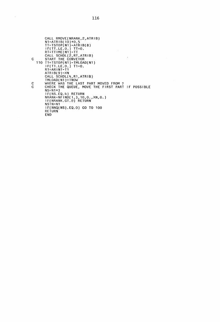
116
CALL RMOVE(NRANK,2,ATRIB) Nl=ATRIB(l0)+0.5 TT=TSTOP(Nl)-ATRIB(8) IF(TT.LE.O.) TT=O. RT=TTIME(Nl)-TT CALL SCHDL(2,RT,ATRIB)
C START THE CONVEYOR 110 Tl=TSTOP(N1)-TMLOAD(Nl)
IF(Tl.LE.O.) T1=0. Rl=AR I NT-T1 ATRIB(9)=XN CALL SCHDL(4,Rl,ATRIB) TMLOAD( Nl )=TNOW
C WHERE WAS THE LAST PART MOVED FROM ? C CHECK THE QUEUE, MOVE THE FIRST PART IF POSSIBLE
NS=N1+3 IF(NS.EQ.4) RETURN NRANK=NFIND(l,3,10,0.,XN,O.) IF(NRANK.GT.O) RETURN NSTN=Nl IF(NNQ(NS).EQ.O) GO TO 100 RETURN END
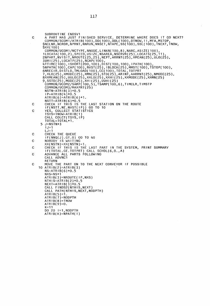
117
SUBROUTINE ENDSVl C A PART HAS JUST FINISHED SERVICE, DETERMINE WHERE DOES IT GO NEXT?
COMMON/SCOMl/ATRI B( 100), DD( 100), DDL( 100), DTNOW, 11, MFA,MSTOP, $NCLNR,NCRDR,NPRNT,NNRUN,NNSET,NTAPE,SS(100),SSL(100),TNEXT,TNOW, $XX(100) .
COMMON/UCOM1/NCTYPE,NNODE,LINKN(100,8),NARC,ASIZE(100), 1LOCATA(100,2),SPEED,USIZE,NSAREA,NSERVR(25),LOCATS(25,11), 2NPART,NVISIT,NROUTE(25,25),NEPT,ARRNT(25),XMEAN(25),UL0(25), 3UHl(25),LOCATP(25),NCAP(100), 4TT IME( 100), I SHORT( 200, 100), DI ST( 100, 100), I PATH( 100), 5NPATH( 100), CAP( 100), NVST( 25), I BLOCK( 25), MMST( 100), TSTOP( 100), 6NRECIR,DISTLD,TMLOAD(100),CC(100),TOTAL,TOTPRT 7,XL0(25),XMODE(25),XMN(25),STD(25),ARINT,AARRNT(25),NMODE(25), 8XXMEAN(25),UUL0(25),XXL0(25),XXHl(25),XXMODE(25),XXMN(25) 9,SSTD(25),MODE(25),XHl(25),UUHl(25)
COMMON/UCOM2/SAMP(100,5),TSAMP(100,6),TIMCLR,TIMSTP COMMON/UCOM3/MAXPRT(25) NSTN=ATRIB(3)+0.5 I P=ATRIB(4)+0.5 ATRIB(6)=ATRIB(6)+1. NSTT=ATRIB(6)+0.5
C CHECK IF THIS IS THE LAST STATION ON THE ROUTE IF(NSTT.NE.NVST( IP)) GO TO 10
C YES, COLLECT STATISTICS TSYS=TNOW-ATRIB(l) CALL COLCT(TSYS, IP) TOTAL=TOTAL+l.
5 J=NSTN+3 IJ=l LJ=l
C CHECK THE QUEUE IF(NNQ(J).GT.O) GO TO 40
c NOBODY rs WAITING XX(NSTN)=XX(NSTN)-1.
C CHECK IF THIS IS THE LAST PART IN THE SYSTEM, PRINT SUMMARY IF(TOTAL.GE.TOTPRT) CALL SCHDL(6,0.,A)
C ADVANCE ALL PARTS FOLLOWING CALL ADVNCl RETURN
C MOVE THE PART ON TO THE NEXT CONVEYOR IF POSSIBLE 10 ATRIB(2)=ATRIB(3)
NS=ATRIB(6)+0.5 NXS=NS+l ATRIB(3)=NROUTE( IP,NXS) NTHIS=ATRIB(2)+0.5 NEXT=ATRIB(3)+0.5 CALL FINDS2(NTHIS,NEXT) CALL PATH(NTHIS,NEXT,NODPTH) ATRIB(5)=1. ATRIB(7)=NODPTH ATRIB(8)=TNOW ATRIB(9)=0. K=l 1 DO 20 1=1,NODPTH ATRIB(K)=NPATH( I)
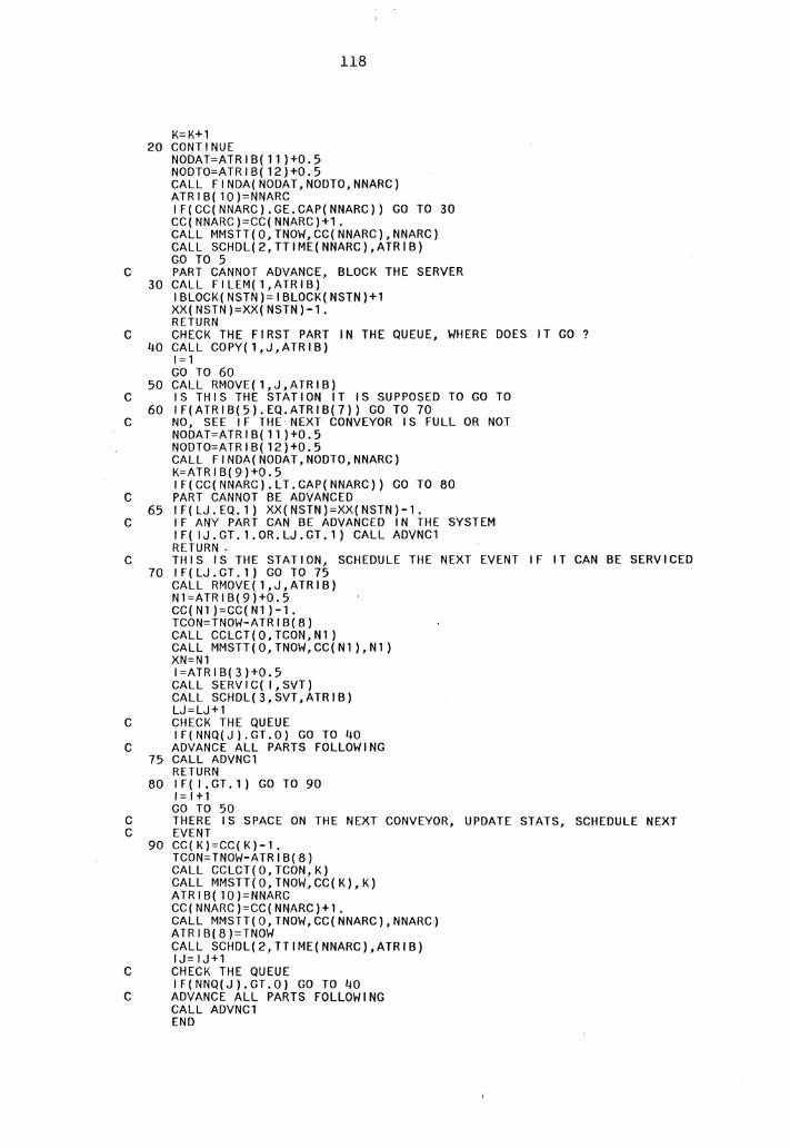
K=K+1 20 CONTINUE
NODAT=ATRIB(11)+0.5 NODTO=ATRIB(12)+0.5
118
CALL FINDA(NODAT,NODTO,NNARC) ATRIB(10)=NNARC IF(CC(NNARC).GE.CAP(NNARC)) GO TO 30 CC(NNARC)=CC(NNARC)+1. CALL MMSTT(O, TNOW,CC(NNARC),NNARC) CALL SCHDL(2,TTIME(NNARC),ATRIB) GO TO 5
C PART CANNOT ADVANCE, BLOCK THE SERVER 30 CALL FILEM(1,ATRIB)
IBLOCK(NSTN)=IBLOCK(NSTN)+1 XX(NSTN)=XX(NSTN)-1. RETURN
C CHECK THE FIRST PART IN THE QUEUE, WHERE DOES IT GO ? 40 CALL COPY(1,J,ATRIB)
1=1 GO TO 60
50 CALL RMOVE(1,J,ATRIB) C IS THIS THE STATION IT IS SUPPOSED TO GO TO
60 IF(ATRIB(5).EQ.ATRIB(7)) GO TO 70 C NO, SEE IF THE NEXT CONVEYOR IS FULL OR NOT
NODAT=ATRIB(1l)+0.5 NODTO=ATRIB(12)+0.5 CALL FINDA(NODAT,NODTO,NNARC) K=ATRIB(9)+0.5 IF(CC(NNARC).LT.CAP(NNARC)) GO TO 80
C PART CANNOT BE ADVANCED 65 IF(LJ.EQ.1) XX(NSTN)=XX(NSTN)-1.
C IF ANY PART CAN BE ADVANCED IN THE SYSTEM IF( IJ.GT.1.0R.LJ.GT.1) CALL ADVNC1 RETURN .
C THIS IS THE STATION, SCHEDULE THE NEXT EVENT IF IT CAN BE SERVICED 70 IF(LJ.GT.1) GO TO 75
CALL RMOVE(1,J,ATRIB) Nl=ATRIB(9)+0.5 CC( N1 )=CC( N1 )-1. TCON=TNOW-ATRIB(8) CALL CCLCT(O,TCON,N1) CALL MMSTT(O, TNOW,CC(N1),N1) XN=N1 l=ATRIB(3)+0.5 CALL SERVIC( l,SVT) CALL SCHDL(3,SVT,ATRIB) LJ=LJ+1
C CHECK THE QUEUE IF(NNQ(J).GT.O) GO TO 40
C ADVANCE ALL PARTS FOLLOWING 75 CALL ADVNC1
RETURN 80 IF( l.GT.1) GO TO 90
1=1+1 GO TO 50
C THERE IS SPACE ON THE NEXT CONVEYOR, UPDATE STATS, SCHEDULE NEXT C EVENT
90 CC(K)=CC(K)-1. TCON=TNOW-ATRIB(8) CALL CCLCT(O,TCON,K) CALL MMSTT(O,TNOW,CC(K),K) ATRIB(10)=NNARC CC(NNARC)=CC(NNARC)+1. CALL MMSTT(O,TNOW,CC(NNARC),NNARC) ATRIB(8)=TNOW CALL SCHDL(2,TTIME(NNARC),ATRIB) IJ=IJ+1
C CHECK THE QUEUE IF(NNQ(J).GT.O) GO TO 40
C ADVANCE ALL PARTS FOLLOWING CALL ADVNC1 END
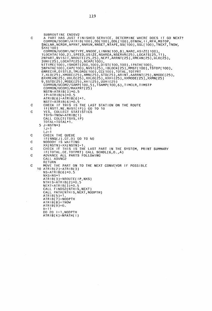
119
SUBROUTINE ENDSV2 C A PART HAS JUST FINISHED SERVICE. DETERMINE WHERE DOES IT GO NEXT?
COMMON/SCOM1/ATRIB(100),DD(100),DDL(100),DTNOW, I l,MFA,MSTOP, $NCLNR,NCRDR,NPRNT,NNRUN,NNSET,NTAPE,SS(100),SSL(100),TNEXT,TNOW, $XX(100)
COMMON/UCOM1/NCTYPE,NNODE,LINKN(100,8),NARC,ASIZE(100), 1LOCATA(100,2),SPEED,USIZE,NSAREA,NSERVR(25),LOCATS(25,11), 2NPART,NVISIT,NROUTE(25,25),NEPT,ARRNT(25),XMEAN(25),UL0(25), 3UHl(25),LOCATP(25),NCAP(100), 4TTIME( 100), I SHORT( 200, 100), DI ST( 100, 100), I PATH( 100), 5NPATH(100),CAP(100),NVST(25), IBLOCK(25),MMST(100),TSTOP(100), 6NRECIR,DISTLD, TMLOAD(100),CC(100),TOTAL,TOTPRT 7,XL0(25),XMODE(25),XMN(25),STD(25),ARINT,AARRNT(25),NMODE(25), 8XXMEAN(25),UUL0(25),XXL0(25),XXHl(25),XXMODE(25),XXMN(25) 9,SSTD(25),MODE(25),XHl(25),UUHl(25)
COMMON/UCOM2/SAMP(100,5),TSAMP(100,6), TIMCLR,TIMSTP COMMON/UCOM3/MAXPRT(25) NSTN=ATRIB(3)+0.5 I P=ATR I B( 4)+0. 5 ATRIB(6)=ATRIB(6)+1. NSTT=ATRIB(6)+0.5
C CHECK IF THIS IS THE LAST STATION ON THE ROUTE IF(NSTT.NE.NVST(IP)) GO TO 10
C YES, COLLECT STATISTICS TSYS=TNOW-ATRIB(1) CALL COLCT(TSYS, IP) TOTAL=TOTAL+1.
5 J=NSTN+3 IJ=1 LJ=1
C CHECK THE QUEUE IF(NNQ(J).GT.O) GO TO 40
C NOBODY IS WAITING XX(NSTN)=XX(NSTN)-1.
C CHECK It THIS IS THE LAST PART IN THE SYSTEM, PRINT SUMMARY IF(TOTAL.GE.TOTPRT) CALL SCHDL(6,0.,A)
C ADVANCE ALL PARTS FOLLOWING CALL ADVNC2 RETURN
C MOVE THE PART ON TO THE NEXT CONVEYOR IF POSSIBLE 10 ATRIB(2)=ATRIB(3)
NS=ATRIB(6)+0.5 NXS=NS+1 ATRIB(3)=NROUTE( IP,NXS) NTHIS=ATRIB(2)+0.5 NEXT=ATRIB(3)+0.5 CALL FINDS2(NTHIS,NEXT) CALL PATH(NTHIS,NEXT,NODPTH) ATRIB(5)=1. ATRIB(7)=NODPTH ATR I B( 8 )=TNOW ATRIB(9)=0. K=l 1 DO 20 1=1,NODPTH ATRIB(K)=NPATH( I)
K=K+1 20 CONTINUE
NODAT=ATRIB(11)+0.5 NODTO=ATRIB(12)+0.5
120
CALL FINDA(NODAT,NODTO,NNARC) ATRIB(10)=NNARC IF(MMST(NNARC).GT.O) GO TO 30 IF(CC(NNARC).GE.CAP(NNARC)) GO TO 30 CC(NNARC)=CC(NNARC)+1. CALL MMSTT(O, TNOW,CC(NNARC),NNARC) IF(CC(NNARC).GT.1.) GO TO 35 CALL SCHDL(2,TTIME(NNARC),ATRIB) GO TO 5
C PART CANNOT ADVANCE, BLOCK THE SERVER 30 CALL FILEM(1,ATRIB)
IBLOCK(NSTN)=IBLOCK(NSTN)+1 XX(NSTN)=XX(NSTN)-1. RETURN
35 CALL FILEM(2,ATRIB) GO TO 5
C CHECK THE FIRST PART IN THE QUEUE, WHERE DOES IT GO ? 40 CALL COPY(1,J,ATRIB)
1=1 GO TO 60
50 CALL RMOVE(1,J,ATRIB) C IS THIS THE STATION IT IS SUPPOSED TO GO TO
60 IF(ATRIB(5).EQ.ATRIB(7)) GO TO 70 C NO, SEE IF THE ~EXT CONVEYOR IS FULL OR NOT
NODAT=ATRIB(11)+0.5 NODTO=ATRIB(12)+0.5 CALL FINDA(NODAT,NODTO,NNARC) K=ATRIB(9)+0.5 IF(MMST(NNARC).GT.O) GO TO 65 IF(CC(NNARC).LT.CAP(NNARC)) GO TO 80
C PART CANNOT BE ADVANCED 65 IF(LJ.EQ.1) XX(NSTN)=XX(NSTN)-1.
C IF ANY PART CAN BE ADVANCED IN THE SYSTEM I F ( I J. GT. 1 . OR. LJ. GT. 1 ) CALL ADVNC2 RETURN
C THIS IS THE STATION, SCHEDULE THE N~XT EVENT IF IT CAN BE SERVICED 70 IF(LJ.GT.1) GO TO 75
CALL RMOVE(1,J,ATRIB) N1=ATRIB(9)+0.5 CC(N1)=CC(N1)-1. TCON=TNOW-ATRIB(8) CALL CCLCT(O,TCON,N1) CALL MMSTT(O,TNOW,CC(N1),N1) XN=N1 MMST(N1)=0 l=ATRIB(3)+0.5 CALL SERVIC( l,SVT) CALL SCHDL(3,SVT,ATRIB) LJ=LJ+1
C CHECK THE QUEUE IF(NNQ(J).GT.O) GO TO 40
121
C ADVANCE ALL PARTS FOLLOWING 75 CALL ADVNC2
RETURN 80 IF( l.GT.1) GO TO 90
1=1+1 GO TO 50
C THERE IS SPACE ON THE NEXT CONVEYOR, UPDATE STATS, SCHEDULE NEXT C EVENT
90 CC(K)=CC(K)-1. TCON=TNOW-ATRIB(8) CALL CCLCT(O,TCON,K) CALL MMSTT(O,TNOW,CC(K),K) ATRIB(10)=NNARC CC(NNARC)=CC(NNARC)+1. CALL MMSTT(O,TNOW,CC(NNARC),NNARC) ATRIB(8)=TNOW IJ= IJ+1 MMST(K)=O IF(CC(NNARC).LE.1.) GO TO 95 CALL FILEM(2,ATRIB) GO TO 96
95 CALL SCHDL(2,TTIME(NNARC),ATRIB) C CHECK THE QUEUE
96 IF(NNQ(J).GT.O) GO TO 40 C ADVANCE ALL PARTS FOLLOWING
GO TO 65 END
122
SUBROUTINE ENDSV3 C A PART HAS JUST FINISHED SERVICE. DETERMINE WHERE DOES IT GO NEXT?
COMMON/SCOM1/ATRIB(100),DD(100),DDL(100),DTNOW, I l,MFA,MSTOP, $NCLNR,NCRDR,NPRNT,NNRUN,NNSET,NTAPE,SS(100),SSL(100),TNEXT,TNOW, $XX(100)
COMMON/UCOM1/NCTYPE,NNODE,LINKN(100,8),NARC,ASIZE(100), 1LOCATA(100,2),SPEED,USIZE,NSAREA,NSERVR(25),LOCATS(25,11), 2NPART,NVISIT,NROUTE(25,25),NEPT,ARRNT(25),XMEAN(25),UL0(25), 3UHl(25),LOCATP(25),NCAP(100), 4TT IME( 100), I SHORT( 200, 100), DI ST( 100, 100), I PATH( 100), 5N PA TH ( 100), CAP( 100), NVST ( 100), I BLOCK( 25), MMST( 100), TSTOP( 100), 6NRECIR,DISTLD,TMLOAD(100),CC(100),TOTAL,TOTPRT 7,XL0(25),XMODE(25),XMN(25),STD(25),ARINT,AARRNT(25),NMODE(25), 8XXMEAN(25),UUL0(25),XXL0(25),XXHl(25),XXMODE(25),XXMN(25) 9,SSTD(25),MODE(25),XHl(25),UUHl(25)
COMMON/UCOM2/SAMP(100,5),TSAMP(100,6),TIMCLR,TIMSTP COMMON/UCOM3/MAXPRT(25) NSTN=ATRIB(3)+0.5 IP=ATRIB(4)+0.5 N1=ATRIB(9)+0.5 ATRIB(6)=ATRIB(6)+1. NSTT=ATRIB(6)+0.5
C CHECK IF THIS IS THE LAST STATION ON THE ROUTE IF(NSTT.NE.NVST( IP)) GO TO 10
C YES, COLLECT STATISTICS TSYS=TNOW-ATRIB(1) CALL COLCT(TSYS, IP) TOTAL=TOTAL+1.
5 J=NSTN+3 C CHECK THE QUEUE
IF(NNQ(J).GT.O) GO TO 30 C NOBODY IS WAITING
XX(NSTN)=XX(NSTN)-1. C CHECK IF.THIS IS THE LAST PART IN THE SYSTEM, PRINT SUMMARY
IF(TOTAL.GE.TOTPRT) CALL SCHDL(6,0.,A) C ADVANCE ALL PARTS FOLLOWING
MMST(N1)=0 CALL ADVNC3 RETURN
C MOVE THE PART ON TO THE NEXT CONVEYOR IF POSSIBLE 10 ATRIB(2)=ATRIB(3)
NS=ATRIB(6)+0.5 NXS=NS+1 ATR I B( 3 )=NROUTE( IP, NXS) NTHIS=ATRIB(2)+0.5 NEXT=ATRIB(3)+0.5 CALL FINDS2(NTHIS,NEXT) CALL PATH(NTHIS,NEXT,NODPTH) ATRIB(5)=1. ATRIB(7)=NODPTH ATRIB(9)=0. K= 11 DO 20 1=1,NODPTH ATRIB(K)=NPATH( I) K=K+1
20 CONTINUE NODAT=ATRIB(11)+0.5 NODTO=ATRIB(12)+0.5
123
CALL flNDA(NODAT,NODTO,NNARC) ATRIB(10)=NNARC
C PART MUST WAIT FOR THE NEXT CONVEYOR LOADING POINT CALL FILEM(3,ATRIB) IBLOCK(NSTN)=IBLOCK(NSTN)+1 XX(NSTN)=XX(NSTN)-1. RETURN
C CHECK THE FIRST PART IN THE QUEUE, WHERE DOES IT GO ? 30 CALL COPY(1,J,ATRIB)
C IS THIS THE STATION IT IS SUPPOSED TO GO TO IF(ATRIB(5).EQ.ATRIB(7)) GO TO 40
C NO C PART CANNOT BE ADVANCED
XX(NSTN)=XX(NSTN)-1. RETURN
C THIS IS THE STATION, SCHEDULE THE NEXT EVENT If IT CAN BE SERVICED 40 CALL RMOVE(1,J,ATRIB)
N1=ATRIB(9)+0.5 CC(Nl)=CC(N1)-1. TCON=TNOW-ATRIB(8) CALL CCLCT(O, TCON,Nl) CALL MMSTT(O,TNOW,CC(N1),N1) MMST(N1)=0 NSTN=ATRIB(3)+0.5 CALL SERVIC(NSTN,SVT) CALL SCHDL(3,SVT,ATRIB)
C ADVANCE ALL PARTS FOLLOWING CALL ADVNC3 RETURN END
124
SUBROUTINE ADVNC1 C A PART AHEAD HAS MOVED IN THE SYSTEM. ALL PARTS FOLLOWING ADVANCE
COMMON/SCOM1/ATRIB(100),DD(100),DDL(100),DTNOW, I l,MFA,MSTOP, $NCLNR,NCRDR,NPRNT,NNRUN,NNSET,NTAPE,SS(100),SSL(100),TNEXT,TNOW, $XX(100)
COMMON/UCOM1/NCTYPE,NNODE,LINKN(100,8),NARC,ASIZE(100), 1LOCATA(100,2),SPEED,USIZE,NSAREA,NSERVR(25),LOCATS(25,11), 2NPART,NVISIT,NROUTE(25,25),NEPT,ARRNT(25),XMEAN(25),UL0(25), 3UHl(25),LOCATP(25),NCAP(100), 4TT I ME( 100), I SHORT( 200, 100), DI ST( 100, 100), I PATH( 100 ), 5NPATH(100),CAP(100),NVST(25), IBLOCK(25),MMST(100),TSTOP(100), 6NRECIR,DISTLD, TMLOAD(100),CC(100),TOTAL,TOTPRT 7,XL0(25),XMODE(25),XMN(25),STD(25),ARINT,AARRNT(25),NMODE(25), 8XXMEAN(25),UUL0(25),XXL0(25),XXHl(25),XXMODE(25),XXMN(25) 9,SSTD(25),MODE(25),XHl(25),UUHl(25)
COMMON/UCOM2/SAMP(100,5),TSAMP(100,6),TIMCLR,TIMSTP COMMON/UCOM3/MAXPRT(25) N1=ATRIB(9)+0.5 XN=N1
C WHERE WAS THE LAST PART MOVED FROM ? 5 NODFR=ATRIB(11)+0.5
IF(ATRIB(9).NE.O .. AND.ATRIB(9).NE.ATRIB(10)) CALL FINDL(NODFR) C WAS THAT A STATION?
6 CALL FINDS(NODFR,NSTN,EX) IJ=1
C WAS THAT STATION ON ITS ROUTE ? IF(ATRIB(9).EQ.O.) GO TO 10 IF(EX.EQ.1.) GO TO 40
C IT WAS ITS OWN STATION OR IT WAS NOT A STATION C CHECK THE QUEUE, MOVE THE FIRST PART IF POSSIBLE
10 NRANK1=NFIND(1,1,10,0.,XN,O.) CN=ATRIB(9) NRANK2=NFIND(1,1,9,0.,CN,O.) IF(NRANK?.EQ.O) GO TO 15 IF(NRANK2.LT.NRANK1) RETURN
15 IF(NRANK1.EQ.O) RETURN C SEE WHERE DOES THE NEXT PART GO
CALL COPY(NRANK1,1,ATRIB) 1=1
20 NODAT=ATRIB(11)+0.5 NOOTO=ATRIB(12)+0.5 CALL FINDA(NODAT,NODTO,NNARC) N1=ATRIB(9)+0.5 ATRIB(10)=NNARC IF(l.GT.1) GO TO 30 IF(CC(NNARC).GE.CAP(NNARC)) RETURN CALL RMOVE(NRANK1,1,ATRIB) I= I +1 GO TO 20
30 CC(NNARC)=CC(NNARC)+1. CALL MMSTT(O,TNOW,CC(NNARC),NNARC) I F ( A TR I B ( 9 ) . NE . 0 . ) CC ( N 1 ) =CC ( N 1 ) - 1 . TCON=TNOW-ATRIB(8) IF( ATR I B( 9). NE. 0.) CALL CCLCT( 0, TCON, N1) IF(ATRIB(9).NE.O) CALL MMSTT(O,TNOW,CC(N1),N1)
125
ATR I B( 8 )=TNOW CALL SCHDL(2, TTIME(NNARC),ATRIB)
C AFTER UPDATING, SEE IF IT IS COMING FROM ITS OWN STATION XN=Nl I F (A TR I B ( 5). GT. 1 . ) GO TO 5
C SEE IF IT WAS BLOCKING ANY SERVER NSTN=ATRIB(2)+0.5 IF( IBLOCK(NSTN).EQ.O) GO TO 5
C FREE THE SERVER IBLOCK(NSTN)=IBLOCK(NSTN)-1
C LAST PART MOVED WAS AT A STATION, NOT ITS OWN 40 J=NSTN+3
NRANK=l IF(NNQ(J).EQ.O) GO TO 10
C SEE WHERE DOES THE NEXT PART IN THE QUEUE GO ? 45 CALL COPY(NRANK,J,ATRIB)
1=1 GO TO 60
50 CALL RMOVE(NRANK,J,ATRIB) C CHECK IF IT IS AT A STATION ON ITS ROUTE
60 IF(ATRIB(5).EQ.ATRIB(7)) GO TO 90 C NO, CHECK THE NEXT CONVEYOR
NODAT=ATRIB(11)+0.5 NODTO=ATRIB(12)+0.5 CALL FINDA(NODAT,NODTO,NNARC) K=ATRIB(9)+0.5 . ATRIB(lO)=NNARC IF(CC(NNARC).LT.CAP(NNARC)) GO TO 70
C THERE IS NO SPACE ON THE NEXT CONVEYOR IF(IJ.GT.1) GO TO 5 GO TO 10
70 I F ( I . GT. 1 ) GO TO 80 l=l+l GO TO 50
C THERE 1g SPACE ON THE NEXT CONVEYOR, UPDATE, & SCHEDULE NEXT EVENT 80 CC(K)=CC(K)-1.
TCON=TNOW-ATRIB(8) CALL CCLCT(O,TCON,K) CALL MMSTT(O,TNOW,CC(K),K) CC(NNARC)=CC(NNARC)+l. CALL MMSTT(O,TNOW,CC(NNARC),NNARC) ATR I B( 8 )=TNOW CALL SCHDL(2,TTIME(NNARC),ATRIB) XN=K IJ=IJ+l
C CHECK THE QUEUE IF(NNQ(J).GT.O) GO TO 40
C ADVANCE ALL PARTS FOLLOWING GO TO 10
C THIS THE STATION, CHECK THE STATUS OF THE SERVERS C SCHEDULE SERVICE IF POSSIBLE
90 IBUSY=IBLOCK(NSTN)+XX(NSTN) IF( IBUSY.GE.NSERVR(NSTN)) GO TO 10 CALL RMOVE(NRANK,J,ATRIB) Nl=ATRIB(9)+0.5 XN=Nl CC( Nl )=CC( Nl )-1. CALL MMSTT(O,TNOW,CC(N1),Nl) TCON=TNOW-ATRIB(8) CALL CCLCT(O, TCON,Nl) XX(NSTN)=XX(NSTN)+l. l=ATRIB(J)+0.5 CALL SERVIC( l,SVT) CALL SCHDL(3,SVT,ATRIB)
C AFTER UPDATING, CHECK THE QUEUE AND ADVANCE ALL PARTS FOLLOWING IF(NNQ(J).GT.O) GO TO 40
GO TO 5 END
126
SUBROUTINE ADVNC2 C A PART AHEAD HAS MOVED IN THE SYSTEM. ALL PARTS FOLLOWING ADVANCE
COMMON/SCOM1/ATRIB(100),DD(100),DDL(100),DTNOW, I l,MFA,MSTOP, $NCLNR,NCRDR,NPRNT,NNRUN,NNSET,NTAPE,SS(100),SSL(100),TNEXT, TNOW, $XX(100)
COMMON/UCOM1/NCTYPE,NNODE,LINKN(100,8),NARC,ASIZE(100), 1LOCATA(100,2),SPEED,USIZE,NSAREA,NSERVR(25),LOCATS(25,11), 2NPART,NVISIT,NROUTE(25,25),NEPT,ARRNT(25),XMEAN(25),UL0(25), 3UHl(25),LOCATP(25),NCAP(100), 4TT I ME( 100), I SHORT( 200, 100), DI ST( 100, 100), I PATH( 100), 5NPATH( 100),CAP( 100),NVST(25), IBLOCK(25),MMST( 100), TSTOP( 100), 6NRECIR,DISTLD,TMLOAD(100),CC(100),TOTAL,TOTPRT 7,XL0(25),XMODE(25),XMN(25),STD(25),ARINT,AARRNT(25),NMODE(25), 8XXMEAN(25),UUL0(25),XXL0(25),XXHl(25),XXMODE(25),XXMN(25) 9,SSTD(25),MODE(25),XHl(25),UUHl(25)
COMMON/UCOM2/SAMP(100,5),TSAMP(100,6),TIMCLR,TIMSTP COMMON/UCOM3/MAXPRT(25)
C SEE IF A PART IS WAITING ON THE CONVEYOR, IF SO ADVANCE IT N1=ATRIB(9)+0.5 XN=N1 NRANK=NFIND(1,2,10,0.,XN,O.) IF(NRANK.EQ.O) GO TO 5 CALL COPY(NRANK,2,ATRIB) IF(MMST(N1).GT.O) GO TO 5 CALL RMOVE(NRANK,2,ATRIB) NODFR=ATRIB(11)+0.5 TT=TSTOP(N1)-ATRIB(8) RT=TTIME(N1 )-TT CALL SCHDL(2,RT,ATRIB) GO TO 6
C WHERE WAS THE LAST PART MOVED FROM ? 5 NODFR=ATRIB(11)+0.5
IF(ATRIB(2).EQ.ATRIB(3)) GO TO 6 IF(ATRIB(9).NE.O .. AND.ATRIB(9).NE.ATRIB(10)) CALL FINDL(NODFR)
C WAS THAT A STATION ? 6 CALL FINDS(NODFR,NSTN,EX)
IJ=1 LJ=1
C WAS THAT STATION ON ITS ROUTE ? I F (A TR I B ( 9). EQ. 0. ) GO TO 10 IF(EX.EQ.1.) GO TO 40
C IT WAS ITS OWN STATION OR IT WAS NOT A STATION C CHECK THE QUEUE, MOVE THE FIRST PART IF POSSIBLE
10 NRANK1=NFIND(1,1,10,0.,XN,O.) CN=ATRIB(9) NRANK2=NFIND(1,1,9,0.,CN,O.) IF(NRANK2.EQ.O) GO TO 15 IF(NRANK2.LT.NRANK1) GO TO 110
15 IF(NRANK1.EQ.O) GO TO 110 C SEE WHERE DOES THE NEXT PART GO
CALL COPY(NRANKl,1,ATRIB) 1=1
20 NODAT=ATRIB(11)+0.5 NODTO=ATRIB(12)+0.5 CALL FINDA(NODAT,NODTO,NNARC)
N1=ATRIB(9)+0.5 ATRIB(10)=NNARC
127
IF( I. GT. 1) GO TO 30 IF(MMST(NNARC).GT.O) GO TO 110 IF(CC(NNARC).GE.CAP(NNARC)) GO TO 110 CALL RMOVE(NRANK1,1,ATRIB) 1=1+1 GO TO 20
30 CC(NNARC)=CC(NNARC)+1. CALL MMSTT(O,TNOW,CC(NNARC),NNARC) I F ( A TR I B ( 9 ) . NE . 0 . ) CC ( N 1 ) =CC ( N 1 ) -1 . TCON=TNOW-ATRIB(8) IF(ATRIB(9).NE.O.) CALL CCLCT(O,TCON,N1) IF(ATRIB(9).NE.O) CALL MMSTT(O,TNOW,CC(N1),N1) ATRIB(8)=TNOW IF(CC(NNARC).LE.1) GO TO 35 CALL FILEM(2,ATRIB) GO TO 36
35 CALL SCHDL(2,TTIME(NNARC),ATRIB) C AFTER UPDATING, SEE IF IT IS COMING FROM ITS OWN STATION
36 XN=N1 MMST(N1)=0 LJ=LJ+1 I F (A TR I B ( 5) . GT. 1 . ) GO TO 10
C SEE IF IT WAS BLOCKING ANY SERVER NSTN=ATRIB(2)+0.5 IF( IBLOCK(NSTN).EQ.O) GO TO 10
C FREE THE SERVER IBLOCK(NSTN)=IBLOCK(NSTN)-1
C LAST PART MOVED WAS AT A STATION, NOT ITS OWN 40 J=NSTN+3
NRANK=1 IF(NNQ(J).EQ.O) GO TO 95
C SEE WHER~ DOES THE NEXT PART IN THE QUEUE GO ? 45 CALL COPY(NRANK,J,ATRIB)
1=1 GO TO 60
50 CALL RMOVE(NRANK,J,ATRIB) C CHECK IF IT IS AT A STATION ON ITS ROUTE
60 IF(ATRIB(5).EQ.ATRIB(7)) GO TO 90 C NO, CHECK THE NEXT CONVEYOR
NODAT=ATRIB(11 )+0.5 NODTO=ATRIB(12)+0.5 CALL FINDA(NODAT,NODTO,NNARC) K=ATRIB(9)+0.5 IF(MMST(K).GT.O) GO TO 65 IF(CC(NNARC).LT.CAP(NNARC)) GO TO 70
C THERE IS NO SPACE ON THE NEXT CONVEYOR 65 IF(IJ.GT.1) GO TO 5
GO TO 10 70 I F ( I . GT. 1 ) GO TO 80
1=1+1 GO TO 50
C THERE IS SPACE ON THE NEXT CONVEYOR, UPDATE, & SCHEDULE NEXT EVENT 80 CC(K)=CC(K)-1.
TCON=TNOW-ATRIB(8) CALL CCLCT(O,TCON,K)
128
CALL MMSTT(O,TNOW,CC(K),K) CC(NNARC)=CC(NNARC)+l. CALL MMSTT(O,TNOW,CC(NNARC),NNARC) ATRIB(8)=TNOW ATR I B( 10 )=NNARC MMST(K)=O IF(CC(NNARC).LE.1.) GO TO 85 CALL FILEM(2,ATRIB) GO TO 86
85 CALL SCHDL(2,TTIME(NNARC),ATRIB) 86 XN=K
IJ=IJ+l C CHECK THE QUEUE
IF(NNQ(J).GT.O) GO TO 40 C ADVANCE ALL PARTS FOLLOWING
GO TO 95 C THIS THE STATION, CHECK THE STATUS OF THE SERVERS C SCHEDULE SERVICE IF POSSIBLE
90 IBUSY=IBLOCK(NSTN)+XX(NSTN) IF( IBUSY.GE.NSERVR(NSTN)) GO TO 95 CALL RMOVE(NRANK,J,ATRIB) Nl=ATRIB(9)+0.5 XN=Nl CC ( N 1 ) =CC ( N 1 ) -1 . MMST(Nl )=O CALL MMSTT(O,TNOW,CC(Nl),Nl) TCON=TNOW-ATRIB(8) CALL CCLCT(O, TCON,Nl) XX(NSTN)=XX(NSTN)+l. IJ= IJ+l IP=ATRIB(3)+0.5 CALL SERVIC( IP,SVT) CALL SCHDL(3,SVT,ATRIB)
C AFTER UPDATING, CHECK THE QUEUE AND ADVANCE ALL PARTS FOLLOWING IF(NNQ(J).GT.0) GO TO 40
95 NRANK=NFIND(l,2,10,0.,XN,O.) IF(NRANK.GT.O) GO TO 100
96 IF(IJ.GT.1) GO TO 5 IF(LJ.LE.1) GO TO 10 RETURN
100 CALL COPY(NRANK,2,ATRIB) Nl=ATRIB(l0)+0.5 IF(MMST(Nl).GT.O) GO TO 96 CALL RMOVE(NRANK,2,ATRIB) Nl=ATR I B( 10 )+O. 5 NODFR=ATRIB(ll)+0.5 TT=TSTOP(Nl)-ATRIB(8) RT=TTIME(N1 )-TT CALL SCHDL(2,RT,ATRIB) I F ( I J. GT. 1 ) GO TO 6
GO TO 10 110 IF(LJ.GT.1) GO TO 95
RETURN END

129
SUBROUTINE ADVNC3 C A PART AHEAD HAS MOVED IN THE SYSTEM. ALL PARTS FOLLOWING ADVANCE
COMMON/SCOM1/ATRIB(100),DD(100),DDL(100),DTNOW, I l,MFA,MSTOP, $NCLNR,NCRDR,NPRNT,NNRUN,NNSET,NTAPE,SS(100),SSL(100),TNEXT,TNOW, $XX(100)
COMMON/UCOM1/NCTYPE,NNODE,LINKN(100,8),NARC,ASIZE(100), 1LOCATA(100,2),SPEED,USIZE,NSAREA,NSERVR(25),LOCATS(25,11), 2NPART,NVISIT,NROUTE(25,25),NEPT,ARRNT(25),XMEAN(25),UL0(25), 3UHl(25),LOCATP(25),NCAP(100), 4TT I ME( 100), I SHORT( 200, 100), DI ST( 100, 100), I PATH( 100), 5NPATH( 100) ,CAP( 100), NVST( 100), I BLOCK( 25), MMST( 100), TSTOP( 100), 6NRECIR,DISTLD,TMLOAD(100),CC(100),TOTAL, TOTPRT 7,XL0(25),XMODE(25),XMN(25),STD(25),ARINT,AARRNT(25),NMODE(25), 8XXMEAN(25),UUL0(25),XXL0(25),XXHl(25),XXMODE(25),XXMN(25) 9,SSTD(25),MODE(25),XH1(25),UUHl(25)
COMMON/UCOM2/SAMP(100,5),TSAMP(100,6),TIMCLR,TIMSTP COMMON/UCOM3/MAXPRT(25)
C SEE IF A PART IS WAITING ON THE CONVEYOR, IF SO ADVANCE IT N1=ATRIB(9)+0.5 XN=N1 IF(MMST(N1 ).GT.O) RETURN NRANK=NFIND(1,2,10,0.,XN,O.) IF(NRANK.EQ.O) GO TO 5 CALL RMOVE(NRANK,2,ATRIB) N1=ATRIB(10)+0.5 TT=TSTOP(N1)-ATRIB(8) IF( TT. LE. 0.) TT=O. RT=TTIME(N1 )-TT CALL SCHDL(2,RT,ATRIB)
C START THE CONVEYOR 5 T1=TSTOP(N1)-TMLOAD(N1)
IF(T1.LE.O.) T1=0. R1=AR I NT-T1 ATRIB(9)~XN CALL SCHDL(4,R1,ATRIB) TMLOAD( N1 )=TNOW
C WHERE WAS THE LAST PART MOVED FROM ? C CHECK THE QUEUE, MOVE THE FIRST PART IF POSSIBLE
6 J=N1+3 IF(J.EQ.4) RETURN NRANK=1
C IF NOTHING IS AT STATION, MOVE THE PARTS ON THE CONVEYOR C FOLLOWING THE STATION.
IF(NNQ(J).EQ.O) GO TO 30 C SEE WHERE DOES THE NEXT PART IN THE QUEUE GO ?
CALL COPY(NRANK,J,ATRIB) C CHECK IF IT IS AT A STATION ON ITS ROUTE
IF(ATRIB(5).EQ.ATRIB(7)) GO TO 10 C NO
RETURN C THIS IS THE STATION, CHECK THE STATUS OF THE SERVERS C SCHEDULE SERVICE IF POSSIBLE
10 IBUSY=IBLOCK(NSTN)+XX(NSTN) I F ( I BUSY. GE. NSERVR ( NSTN) ) RETURN CALL RMOVE(NRANK,J,ATRIB)
Nl=ATRIB(9)+0.5 XN=N1 CC(N1)=CC(N1)-1. MMST(Nl)=O
130
CALL MMSTT(O,TNOW,CC(Nl),Nl) TCON=TNOW-ATRIB(8) CALL CCLCT(O,TCON,Nl) XX(NSTN)=XX(NSTN)+1. NSTN=ATRIB(J)+0.5 CALL SERVIC(NSTN,SVT) CALL SCHDL(J,SVT,ATRIB)
C AFTER UPDATING, ADVANCE ALL PARTS FOLLOWING IF(MMST(Nl).GT.O) RETURN NRANK=NFIND(l,2,10,0.,XN,O.) IF(NRANK.GT.O) GO TO 20 GO TO 5
20 CALL RMOVE(NRANK,2,ATRIB) Nl=ATRIB(10)+0.5 TT=TSTOP(Nl)-ATRIB(8) RT=TTIME(N1 )-TT CALL SCHDL(2,RT,ATRIB)
C START THE CONVEYOR T1=TSTOP(N1)-TMLOAD(N1) IF( T1. LE. 0.) Tl=O. Rl=AR I NT-Tl ATRIB(9)=N1 CALL SCHDL(4,R1,ATRIB) TMLOAD(Nl)=TNOW GO TO 6
C MOVE PARTS ON PRECEEDING CONVEYORS IF POSSIBLE 30 NSTN=N1 40 Nl=NSTN-1
MMST(Nl )=O XN=Nl NRANK=NFIND(l,2,10,0.,XN,0.) IF(NRANK.EQ.O) GO TO 50 CALL RMOVE(NRANK,2,ATRIB) N1=ATRIB(10)+0.5 TT=TSTOP(N1)-ATRIB(8) IF( TT. LE.O.) TT=O. RT=TTIME(N1 )-TT CALL SCHDL(2,RT,ATRIB)
C START THE CONVEYOR 50 Tl=TSTOP(N1)-TMLOAD(N1)
IF( T1. LE. 0.) Tl=O. R1=AR I NT-Tl ATRIB(9)=XN CALL SCHDL(4,R1,ATRIB) TMLOAD( N1 )=TNOW
C WHERE WAS THE LAST PART MOVED FROM ? C CHECK THE QUEUE, MOVE THE FIRST PART IF POSSIBLE
NS=N1+3 IF(NS.EQ.4) RETURN NRANK=NFIND(l,3,10,0.,XN,O.) IF(NRANK.GT.O) RETURN NSTN=N1 IF(NNQ(NS).EQ.O) GO TO 40 RETURN END
131
SUBROUTINE CLRST C CLEAR STATISTICS AFTER THE DESIGNATED TIME
COMMON/SCOMl/ATRIB(lOO),DD(lOO),DDL(lOO),DTNOW, I l,MFA,MSTOP, $NCLNR,NCRDR,NPRNT,NNRUN,NNSET,NTAPE,SS(100),SSL(100),TNEXT,TNOW, $XX(100) COMMON/UCOMl/NCTYPE,NNODE,LINKN(l00,8),NARC,ASIZE(lOO),
1LOCATA(l00,2),SPEED,USIZE,NSAREA,NSERVR(25),LOCATS(25,11), 2NPART,NVISIT,NROUTE(25,25),NEPT,ARRNT(25),XMEAN(25),UL0(25), 3UHl(25),LOCATP(25),NCAP(l00), 4TT IME( 100), I SHORT( 200, 100), DI ST( 100, 100), I PATH( 100), 5NPATH( 100), CAP( 100), NVST( 25), I BLOCK( 25), MMST( 100), TSTOP( 100), 6NRECIR,DISTLD,TMLOAD(lOO),CC(lOO),TOTAL,TOTPRT 7,XL0(25),XMODE(25),XMN(25),STD(25),ARINT,AARRNT(25),NMODE(25), 8XXMEAN(25),UUL0(25),XXL0(25),XXHl(25),XXMODE(25),XXMN(25) 9,SSTD(25),MODE(25),XHl(25),UUHl(25)
COMMON/UCOM2/SAMP(100,5),TSAMP(100,6),TIMCLR,TIMSTP COMMON/UCOM3/MAXPRT(25) CALL CLEAR CALL CCLCT(-1,X,NARC) CALL MMSTT(-1,TNOW,CC(NARC),NARC)
C RE-INITIALIZE THE STATISTICS OF TIME PERSISTENT VARIABLES DO 10 1=1, NARC I F(CC( I ).GT.O.) CALL MMSTT(O, TNOW,CC( I), I)
10 CONT I NUE RETURN END
132
SUBROUTINE SMMRY C PRINT SUMMARY
COMMON/SCOM1/ATRIB(100),00(100),00L(100),DTNOW, I l,MFA,MSTOP, $NCLNR,NCROR,NPRNT,NNRUN,NNSET,NTAPE,SS(100),SSL(100),TNEXT,TNOW, $XX(100)
COMMON/UCOM1/NCTYPE,NNODE,LINKN(100,8),NARC,ASIZE(100), 1LOCATA(100,2),SPEED,USIZE,NSAREA,NSERVR(25),LOCATS(25,11), 2NPART,NVISIT,NROUTE(25,25),NEPT,ARRNT(25),XMEAN(25),UL0(25), 3UHl(25),LOCATP(25),NCAP(100), 4TT I ME( 100), I SHORT( 200, 100), 0 I ST( 100, 100), I PATH( 100), 5NPATH( 100), CAP( 100), NVST( 25), I BLOCK( 25), MMST( 100), TSTOP( 100), 6NRECIR,DISTLD, TMLOAD(100),CC(100),TOTAL,TOTPRT 7,XL0(25),XMODE(25),XMN(25),ST0(25),ARINT,AARRNT(25),NMODE(25), 8XXMEAN(25),UUL0(25),XXL0(25),XXHl(25),XXMODE(25),XXMN(25) 9,SSTD(25),MODE(25),XHl(25),UUHl(25)
COMMON/UCOM2/SAMP(100,5),TSAMP(100,6), TIMCLR,TIMSTP COMMON/UCOM3/MAXPRT(25) WRITE(6, 180) DO 10 1=1,NARC CALL CCLCT(1,A, I)
10 CONTINUE WRITE(6,190) DO 20 1=1,NARC CALL MMSTT( 1, TNOW,CC( I), I)
20 CONTINUE MSTOP=-1 RETURN
180 FORMAT(///,32X, '**STATISTICS FOR VARIABLES BASED ON OBSERVATION $**' ,//,22X, 'MEAN' ,9X, 'STANDARD' ,6X, 'COEFF.OF' ,5X, 'MINIMUM' ,7X, 'MA $XIMUM' ,6X, 'NUMBER OF' ,/,22X, 'VALUE' ,8X, 'DEVIATION' ,5X,'VARIATION', $5X, 'VALUE' ,9X, 'VALUE' ,8X, 'OBSERVATIONS',/)
190 FORMAT(///,32X, '**STATISTICS FOR TIME-PERSISTENT VARIABLES $**' ,//,22X, 'MEAN' ,9X, 'STANDARD' ,6X, 'MINIMUM', 7X, 'MAXIMUM' ,7X, 'TIME $' ,10X, 'CURRENT',/,22X, 'VALUE' ,8X,'DEVIATION' ,5X, 'VALUE',9X, 1 VALUE' $,9X, I INTERVAL' ,6X, 'VALUE',/)
END
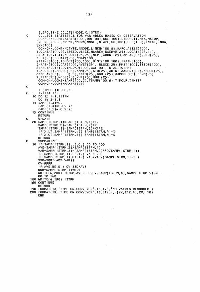
133
SUBROUTINE CCLCT( IMODE,X, ISTRM) C COLLECT STATISTICS FOR VARIABLES BASED ON OBSERVATION
c
COMMON/SCOM1/ATRIB(100),DD(100),DDL(100),DTNOW, I l,MFA,MSTOP, $NCLNR,NCRDR,NPRNT,NNRUN,NNSET,NTAPE,SS(100),SSL(100),TNEXT,TNOW, $XX(100) .
COMMON/UCOM1/NCTYPE,NNODE,LINKN(100,8),NARC,ASIZE(100), 1LOCATA(100,2),SPEED,USIZE,NSAREA,NSERVR(25),LOCATS(25,11), 2NPART,NVISIT,NROUTE(25,25),NEPT,ARRNT(25),XMEAN(25),UL0(25), 3UHl(25),LOCATP(25),NCAP(100), 4 TT I ME ( 1 00), I SHORT ( 200, 100), DI ST ( 1 00, 1 00), I PA TH ( 1 00), 5NPATH( 100), CAP( 100), NVST( 25), I BLOCK( 25), MMST( 100), TSTOP( 100), 6NRECIR,DISTLD,TMLOAD(100),CC(100),TOTAL,TOTPRT 7,XL0(25),XMODE(25J,XMN(25),STD(25),ARINT,AARRNT(25),NMODE(25), 8XXMEAN(25),UUL0(25),XXL0(25),XXHl(25),XXMODE(25);XXMN(25) 9,SSTD(25),MODE(25),XHl(25),UUHl(25)
COMMON/UCOM2/SAMP(100,5),TSAMP(100,6),TIMCLR,TIMSTP COMMON/UCOM3/MAXPRT(25)
IF( IMODE)10,20,30 C INITIALIZE
10 DO 15 I= 1 , I STRM DO 14 J=1,3
14 SAMP( I ,J )=O. SAMP( I ,4)=0.09E75 SAMP( 1,5)=-0.9E75
15 CONTINUE RETURN
C UPDATE 20 SAMP( I STRM, 1 )=SAMP( I STRM, 1 )+1.
SAMP( ISTRM,2)=SAMP( ISTRM,2)+X SAMP( ISTRM,3)=SAMP( ISTRM,3)+X**2 IF(X.LT.SAMP( ISTRM,4)) SAMP( ISTRM,4)=X IF(X.GT.SAMP( ISTRM,5)) SAMP( ISTRM,5)=X RETURN
C SUMMARIZE 30 IF(SAMP(ISTRM,1).LE.O.) GO TO 100
AVE=SAMP( ISTRM,2)/SAMP( ISTRM,1) VAR=SAMP( ISTRM,3)-(SAMP( ISTRM,2)**2/SAMP( ISTRM,1)) IF( SAMP( I STRM, 1). LE. 1.) VAR=O. 0 IF( SAMP( I STRM, 1). GT. 1. ) VAR=VAR/( SAM.P( I STRM, 1 )-1. ) SSD=SQRT(ABS(VAR)) CV=9999. IF(AVE.NE.O.) CV=SSD/AVE NOB=SAMP( ISTRM,1)+0.5 WRITE(6,200) ISTRM,AVE,SSD,CV,SAMP( ISTRM,4),SAMP( ISTRM,5),NOB GO TO 160
1 00 WR I TE ( 6, 190) I STRM 160 CONTINUE
RETURN 190 FORMAT(1X, 'TIME ON CONVEYOR', 13,17X, 'NO VALUES RECORDED') 200 FORMAT( 1X, 1 TI ME ON CONVEYOR', 13, E12. 4, 4( 2X, E12. 4), 2X, 110)
END
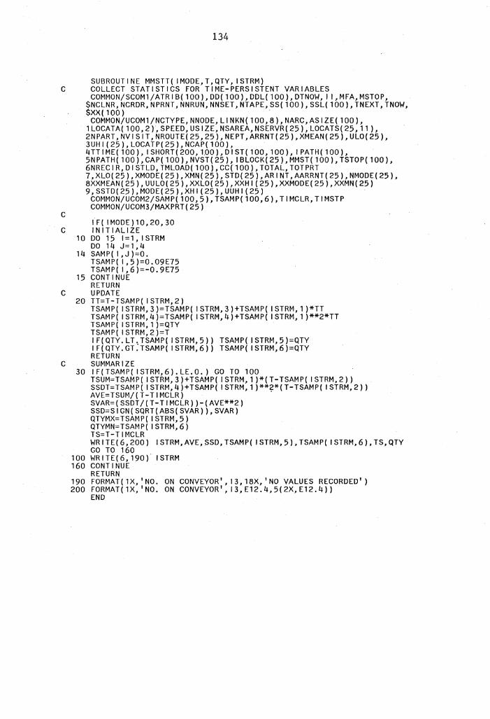
134
SUBROUTINE MMSTT( IMODE,T,QTY, ISTRM) C COLLECT STATISTICS FOR TIME-PERSISTENT VARIABLES
c
COMMON/SCOM1/ATRIB(100),DD(100),DDL(100),DTNOW, I l,MFA,MSTOP, $NCLNR,NCRDR,NPRNT,NNRUN,NNSET,NTAPE,SS(100),SSL(100),TNEXT,TNOW, $XX(100) .
COMMON/UCOM1/NCTYPE,NNODE,LINKN(100,8),NARC,ASIZE(100), 1LOCATA(100,2)~SPEED,USIZE,NSAREA,NSERVR(25),LOCATS(25,11 ), 2NPART,NVISIT,NROUTE(25,25),NEPT,ARRNT(25),XMEAN(25),UL0(25), 3UHl(25),LOCATP(25),NCAP(100), 4TT IME( 100), I SHORT( 200, 1.00), DI ST( 100, 100), I PATH( 100), 5NPATH( 100), CAP( 100), NVST( 25), I BLOCK( 25), MMST( 100), TSTOP( 100), 6NRECIR,DISTLD,TMLOAD(100),CC(100),TOTAL,TOTPRT 7,XL0(25),XMODE(25),XMN(25),STD(25),ARINT,AARRNT(25),NMODE(25), 8XXMEAN(25),UUL0(25),XXL0(25),XXHl(25),XXMODE(25),XXMN(25) 9,SSTD(25),MODE(25),XHl(25),UUHl(25)
COMMON/UCOM2/SAMP(100,5),TSAMP(100,6),TIMCLR,TIMSTP COMMON/UCOM3/MAXPRT(25)
IF( IMODE)10,20,30 C INITIALIZE
10 DO 15 I= 1, I STRM D014J=l,4
14 SAMP( I, J )=O. TSAMP( l,5)=0.09E75 TSAMP( l,6)=-0.9E75
15 CONTINUE RETURN
C UPDATE 20 TT=T-TSAMP( ISTRM,2)
TSAMP( ISTRM,3)=TSAMP( ISTRM,3)+TSAMP( ISTRM,1)*TT TSAMP( ISTRM,4)=TSAMP( ISTRM,4)+TSAMP( ISTRM,1)**2*TT TSAMP( ISTRM,1)=QTY TSAMP( ISTRM,2)=T IF(QTY.LT,TSAMP( ISTRM,5)) TSAMP( ISTRM,5)=QTY IF(QTY.GT.TSAMP( ISTRM,6)) TSAMP( ISTRM,6)=QTY RETURN
C SUMMARIZE 30 IF(TSAMP(ISTRM,6).LE.O.) GO TO 100
TSUM=TSAMP( ISTRM,3)+TSAMP( ISTRM,1)*(T-TSAMP( ISTRM,2)) SSDT=TSAMP( ISTRM,4)+TSAMP( ISTRM,l)**?*(T-TSAMP( ISTRM,2)) AVE=TSUM/(T-TIMCLR) SVAR=(SSDT/(T-TIMCLR))-(AVE**2) SSD=SIGN(SQRT(ABS(SVAR)),SVAR) QTYMX=TSAMP( ISTRM,5) QTYMN=TSAMP( ISTRM,6) TS=T-TIMCLR WRITE(6,200) ISTRM,AVE,SSD, TSAMP( ISTRM,5), TSAMP( ISTRM,6), TS, QTY GO TO 160
100 WRITE(6, 190) ISTRM 160 CONTINUE
RETURN 190 FORMAT(1X, 'NO. ON CONVEYOR', 13,18X, 'NO VALUES RECORDED') 200 FORMAT(1X, 1 NO. ON CONVEYOR',13,E12.4,5(2X,E12.4))
END
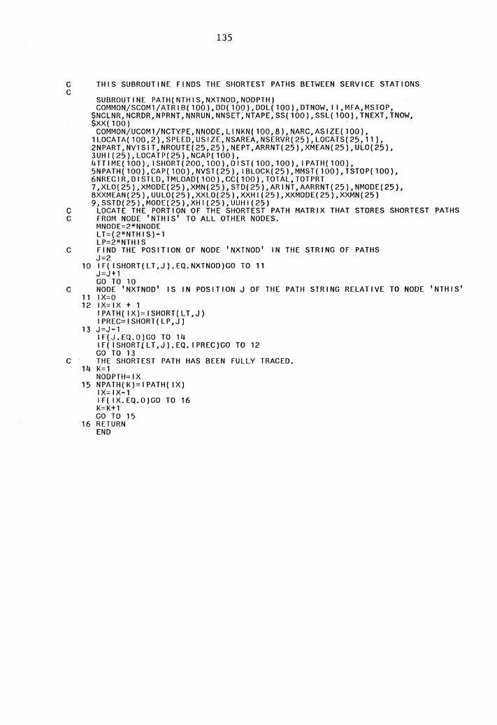
135
C THIS SUBROUTINE FINDS THE SHORTEST PATHS BETWEEN SERVICE STATIONS c
SUBROUTINE PATH(NTHIS,NXTNOD,NODPTH) COMMON/SCOM1/ATRIB(100),DD(100),DDL(100),DTNOW, I l,MFA,MSTOP,
$NCLNR,NCRDR,NPRNT,NNRUN,NNSET,NTAPE,SS(100),SSL(100),TNEXT,TNOW, $XX(100)
COMMON/UCOM1/NCTYPE,NNODE,LINKN{100,8),NARC,ASIZE(100), 1LOCATA(100,2),SPEED,USIZE,NSAREA,NSERVR(25),LOCATS(25,11), 2NPART,NVISIT,NROUTE(25,25),NEPT,ARRNT(25),XMEAN(25),UL0(25), 3UHl(25),LOCATP(25),NCAP(100), 4TT IME( 100), I SHORT( 200, 100), DI ST( 100, 100), I PATH( 100), 5NPATH(100),CAP(100),NVST(25), IBLOCK(25),MMST(100),TSTOP(100), 6NRECIR,DISTLD,TMLOAD(lOO),CC(100),TOTAL,TOTPRT 7,XL0(25),XMODE(25),XMN(25),STD(25),ARINT,AARRNT(25),NMODE(25), 8XXMEAN(25),UUL0(25),XXL0(25),XXHl(25),XXMODE(25),XXMN(25) 9,SSTD(25),MODE(25),XHl(25),UUHl(25)
C LOCATE THE PORTION OF THE SHORTEST PATH MATRIX THAT STORES SHORTEST PATHS C FROM NODE 'NTHIS' TO ALL OTHER NODES.
MNODE=2*NNODE . LT=(2*NTHIS)-1 LP=2*NTHIS
C FIND THE POSITION OF NODE 'NXTNOD' IN THE STRING OF PATHS J=2
10 IF( ISHORT(LT,J).EQ.NXTNOD)GO TO 11 J=J+1 GO TO 10
C NODE 'NXTNOD 1 IS IN POSITION J OF THE PATH STRING RELATIVE TO NODE 'NTHIS' 11 I X=O 12 IX=IX + 1
IPATH( IX)=ISHORT(LT,J) IPREC=ISHORT(LP,J)
13 J=J-1 IF(J.EQ.O)GO TO 14 IF( ISHORTiLT,J).EQ. IPREC)GO TO 12
GO TO 13 C THE SHORTEST PATH HAS BEEN FULLY TRACED.
14 K=1 NODPTH=IX
15 NPATH(K)=IPATH( IX) IX=IX-1 IF( IX. EQ.O)GO TO 16 K=K+l GO TO 15
16 RETURN END

APPENDIX B
EXAMPLES
136
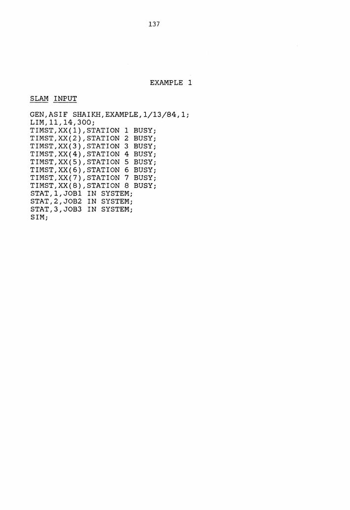
137
EXAMPLE 1
SLAM INPUT
GEN,ASIF SHAIKH,EXAMPLE,l/13/84,l; LIM,11,14,300; TIMST,XX(l},STATION 1 BUSY; TIMST,XX(2},STATION 2 BUSY; TIMST,XX(3},STATION 3 BUSY; TIMST,XX(4},STATION 4 BUSY; TIMST,XX(S},STATION 5 BUSY; TIMST,XX(6},STATION 6 BUSY; TIMST,XX(7},STATION 7 BUSY; TIMST,XX(B},STATION 8 BUSY; STAT,l,JOBl IN SYSTEM; STAT,2,JOB2 IN SYSTEM; STAT,3,JOB3 IN SYSTEM; SIM;
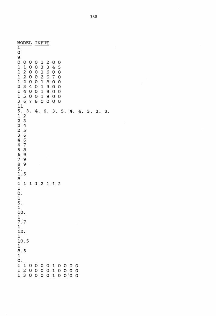
138
MODEL INPUT 1 0 9 0 0 0 0 1 2 0 0 1 1 0 0 3 3 4 5 1 2 0 0 1 6 0 0 1 2 0 0 2 6 7 0 1 2 0 0 1 8 0 0 2 3 4 0 1 9 0 0 1 4 0 0 1 9 0 0 1 5 0 0 1 9 0 0 3 6 7 8 0 0 0 0 11 5. 3. 4. 6. 3 . 5. 4. 4. 3. 3. 3. 1 2 2 3 2 4 2 5 3 6 4 6 4 7 5 8 6 9 7 9 8 9 5. 1. 5 8 1 1 1 1 2 1 1 2 1 0. 1 5. 1 10. 1 7.7 1 12. 1 10.5 1 8.5 1 0. 1 1 0 0 0 0 1 0 0 0 0 1 2 0 0 0 0 1 0 0 0 0 1 3 0 0 0 0 1 0 o·o 0
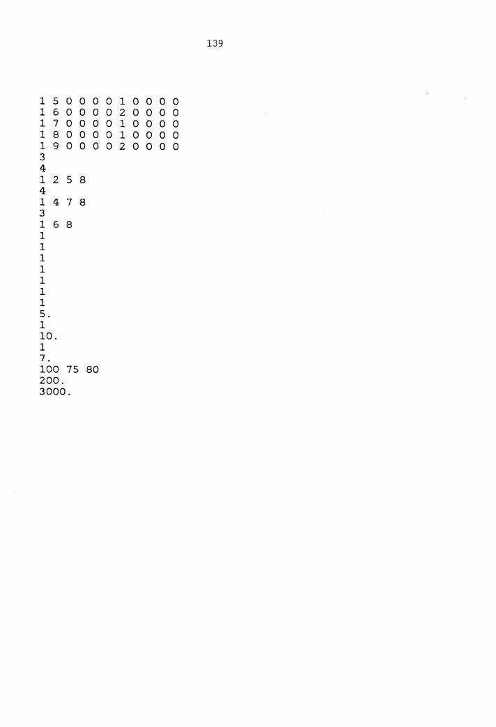
139
1 5 0 0 0 0 1 0 0 0 0 1 6 0 0 0 0 2 0 0 0 0 1 7 0 0 0 0 1 0 0 0 0 1 8 0 0 0 0 1 0 0 0 0 1 9 0 0 0 0 2 0 0 0 0 3 4 1 2 5 8 4 1 4 7 8 3 1 6 8 1 1 1 1 1 1 1 5. 1 10. 1 7. 100 75 80 200. 3000.
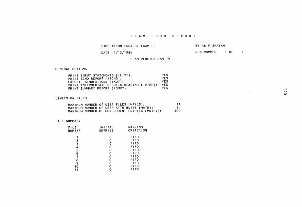
GENERAL OPTIONS
S L A M E C H O
SIMULATION PROJECT EXAMPLE
DATE 1/13/1984 SLAM VERSION jAN 79
PRINT INPUT STATEMENTS ( ILIST): YES PRINT ECHO REPORT (!ECHO): YES EXECUTE SIMULATIONS ( IXQT): YES PRINT INTERMEDIATE RESULTS HEADING ( IPIRH): YES PRINT SUMMARY REPORT ( ISMRY): YES
LIMITS ON FILES
R E P 0 R T
MAXIMUM NUMBER OF USER FILES (MFILS): 11 MAXIMUM NUMBER OF USER ATTRIBUTES (MATR): 14 MAXIMUM NUMBER OF CONCURRENT ENTRIES (MNTRY): 300
FILE SUMMARY
FILE INITIAL RANKING NUMBER ENTRIES CRITERION
1 0 Fl FO 2 0 FIFO 3 0 FIFO 4 0 FIFO 5 0 FIFO 6 0 FIFO 7 0 Fl FO 8 0 FIFO 9 0 FIFO
10 0 FIFO 11 0 FIFO
BY ASIF SHAIKH
RUN NUMBER OF
I-' -l:' 0
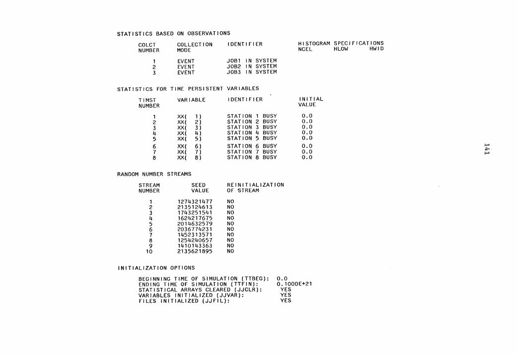
STATISTICS BASED ON OBSERVATIONS
COLCT NUMBER
1 2 3
COLLECTION MODE
EVENT EVENT EVENT
IDENTIFIER
JOB1 IN SYSTEM JOB2 IN SYSTEM JOB3 IN SYSTEM
STATISTICS FOR TIME PERSISTENT VARIABLES
TIMST VARIABLE IDENTIFIER NUMBER
1 XX( 1 ) STATION 1 BUSY 2 XX( 2) STATION 2 BUSY 3 XX( 3) STATION 3 BUSY 4 XX( 4) STATION 4 BUSY
HISTOGRAM SPECIFICATIONS NCEL HLOW HWID
INITIAL VALUE
0.0 0.0 0.0 0.0
5 XX( 5) STATION 5 BUSY 0.0 6 XX( 6) STATION 6 BUSY 0.0 7 XX( 7) STATION 7 BUSY 0.0 8 XX( 8) STATION 8 BUSY o.o
RANDOM NUMBER STREAMS
STREAM SEED REINITIALIZATION NUMBER VALUE OF STREAM
1 1274321477 NO 2 2135124613 NO 3 1743251541 NO 4 1624217675 NO 5 2014632579 NO 6 2036774231 NO 7 1452313571 NO 8 1254240657 NO 9 1410143363 NO
10 2135621895 NO
INITIALIZATION OPTIONS
BEGINNING TIME OF SIMULATION (TTBEG): ENDING TIME OF SIMULATION (TTFIN): STATISTICAL ARRAYS CLEARED (JJCLR): VARIABLES INITIALIZED (JJVAR): FILES INITIALIZED (JJFIL):
0.0 0.1000E+21
YES YES YES
I-' .i:-1-'
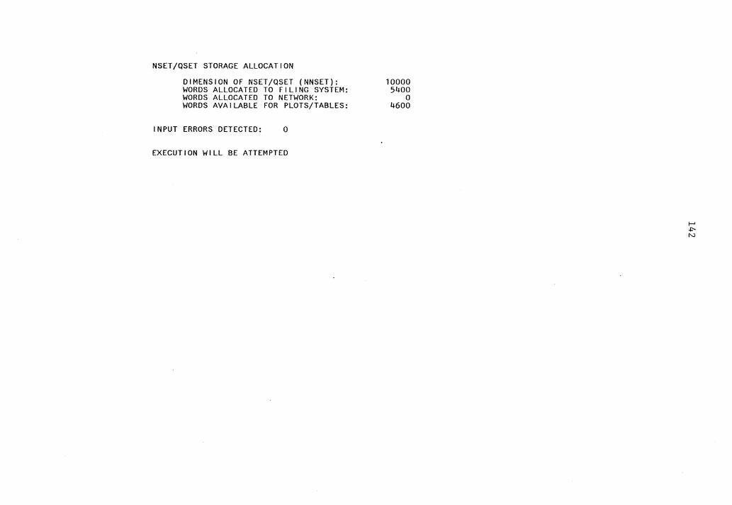
NSET/QSET STORAGE ALLOCATION
DIMENSION OF NSET/QSET (NNSET): WORDS ALLOCATED TO FILING SYSTEM: WORDS ALLOCATED TO NETWORK: WORDS AVAILABLE FOR PLOTS/TABLES:
INPUT ERRORS DETECTED: 0
EXECUTION WILL BE ATTEMPTED
10000 5400
0 4600
f-' -"" N
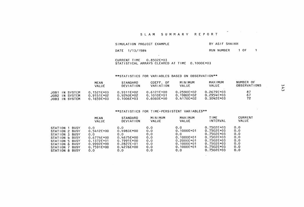
MEAN VALUE
JOBl IN SYSTEM 0.1521E+03 JOB2 IN SYSTEM 0.9151E+02 JOB3 IN SYSTEM 0. 1659E+03
MEAN VALUE
STATION 1 BUSY o.o STATION 2 BUSY 0.5412E+OO STATION 3 BUSY 0.0 STATION 4 BUSY 0. 6774E+OO STATION 5 BUSY 0.1372E+01 STATION 6 BUSY 0.9992E+OO STATION 7 BUSY 0.7591E+OO STATION 8 BUSY o.o
S L A M S U M M A R Y R E P 0 R T
SIMULATION PROJECT EXAMPLE
DATE 1/13/1984
BY ASIF SHAIKH
RUN NUMBER OF
CURRENT TIME 0.8502E+03 STATISTICAL ARRAYS CLEARED AT TIME 0.1000E+03
**STATISTICS FOR VARIABLES BASED ON OBSERVATION**
STANDARD COEFF. OF MINIMUM MAXIMUM NUMBER OF DEVIATION VARIATION VALUE VALUE OBSERVATIONS
0.9311E+02 0.6121E+OO 0.2590E+02 0.2679E+03 87 0.9240E+02 0. 1010E+01 0.1980E+02 0.2954E+03 67 0. 1006E+03 0.6060E+OO 0.4170E+02 0.3042E+03 72
**STATISTICS FOR TIME-PERSISTENT VARIABLES**
STANDARD MINIMUM MAXIMUM TIME CURRENT DEVIATION VALUE VALUE INTERVAL VALUE
o.o 0.0 0.0 0.7502E+03 o.o 0.4983E+OO o.o O. lOOOE+Ol 0.7502E+03 0.0 o.o o.o o.o 0.7502E+03 0.0 0.4675E+OO 0.0 0.1000E+01 0.7502E+03 0.0 0.7991E+OO o.o 0.2000E+01 0.7502E+03 o.o 0.2827E-01 0.0 0. 1000E+01 0.7502E+03 0.0 0.4276E+OO 0.0 O.lOOOE+Ol 0.7502E+03 0.0 0.0 o.o o.o 0.7502E+03 0.0
I-' +:-w
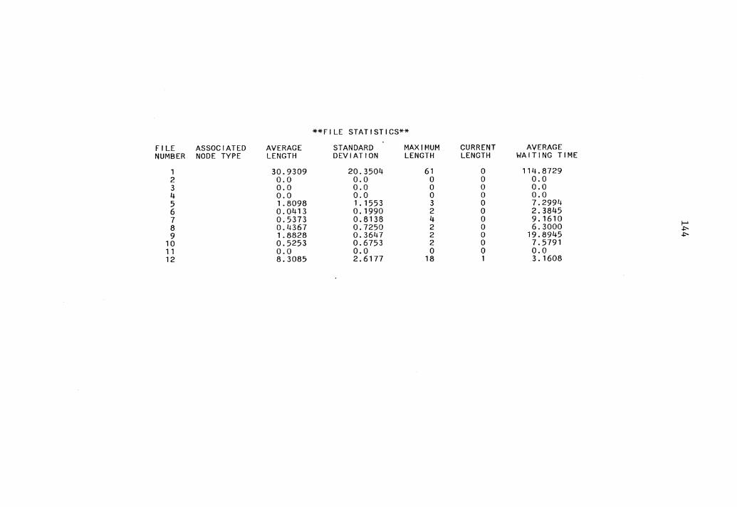
**FILE STATISTICS**
FILE ASSOCIATED AVERAGE STANDARD MAXIMUM CURRENT AVERAGE NUMBER NODE TYPE LENGTH DEVIATION LENGTH LENGTH WAITING TIME
1 30.9309 20.3504 61 0 114.8729 2 0.0 0.0 0 0 0.0 3 0.0 0.0 0 0 0.0 4 0.0 0.0 0 0 0.0 5 1.8098 1 . 1553 3 0 7.2994 6 0.0413 0.1990 2 0 2. 3845 7 0.5373 0.8138 4 0 9.1610 8 0.4367 0.7250 2 0 6.3000 I-' ..,... 9 1. 8828 0.3647 2 0 19.8945 ..,...
10 0.5253 0.6753 2 0 7.5791 11 0.0 0.0 0 0 0.0 12 8.3085 2.6177 18 1 3. 1608
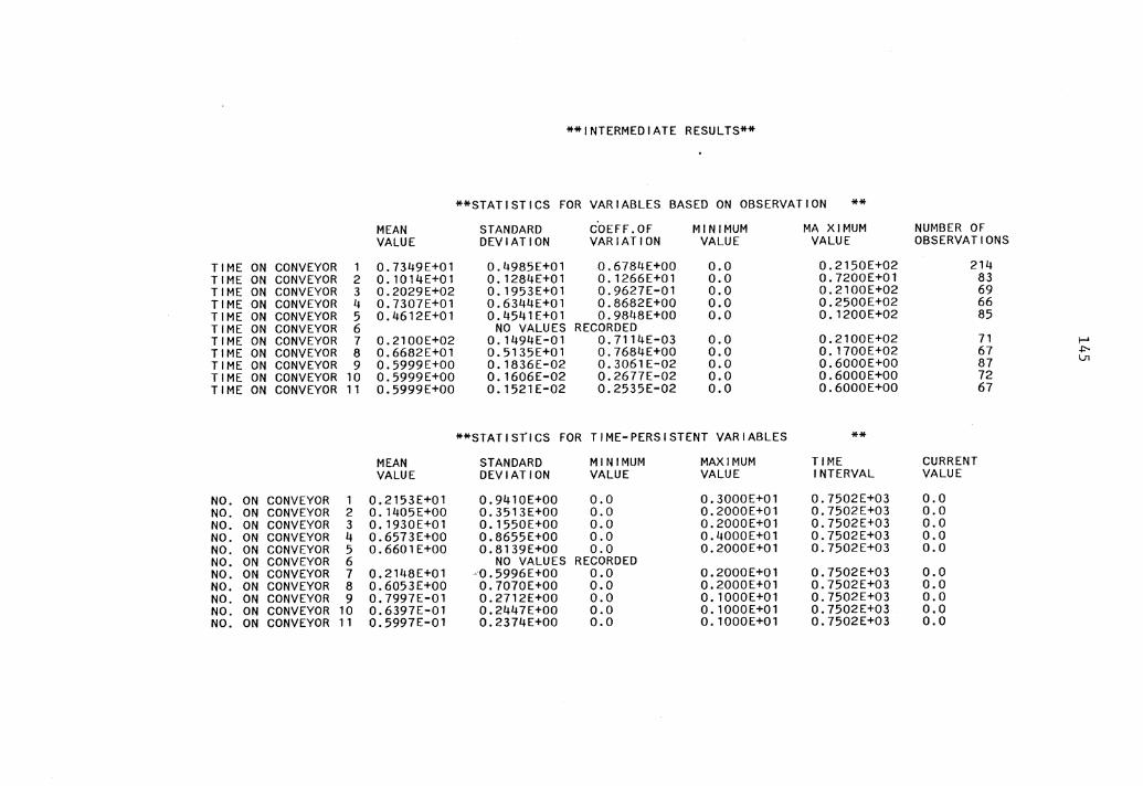
**INTERMEDIATE RESULTS**
**STATISTICS FOR VARIABLES BASED ON OBSERVATION **
MEAN STANDARD COEFF .OF MINIMUM MAXIMUM NUMBER OF VALUE DEVIATION VARIATION VALUE VALUE OBSERVATIONS
TIME ON CONVEYOR 1 0.7349E+01 0.4985E+01 0.6784E+OO 0.0 0.2150E+02 214 TIME ON CONVEYOR 2 0.1014E+01 0.1284E+01 0. 1266E+01 0.0 0.7200E+01 83 TIME ON CONVEYOR 3 0.2029E+02 0.1953E+01 0.9627E-01 0.0 0.2100E+02 69 TIME ON CONVEYOR 4 0. 7307E+01 0.6344E+01 0.8682E+OO 0.0 0.2500E+02 66 TIME ON CONVEYOR 5 0.4612E+01 0.4541E+01 0.9848E+OO 0.0 0.1200E+02 85 TIME ON CONVEYOR 6 NO VALUES RECORDED TIME ON CONVEYOR 7 0.2100E+02 0. 1494E-01 0.7114E-03 0.0 0.2100E+02 71 f-' TIME ON CONVEYOR 8 0.6682E+01 0.5135E+01 0.7684E+OO 0.0 0. 1700E+02 67 +:--TIME ON CONVEYOR 9 0.5999E+OO 0.1836E-02 0.3061E-02 0.0 0.6000E+OO 87 Vl
TIME ON CONVEYOR 10 0.5999E+OO 0.1606E-02 0.2677E-02 0.0 0.6000E+OO 72 TIME ON CONVEYOR 11 0.5999E+OO 0.1521E-02 0.2535E-02 0.0 0.6000E+OO 67
**STATISTICS FOR TIME-PERSISTENT VARIABLES **
MEAN STANDARD MINIMUM MAXIMUM TIME CURRENT VALUE DEVIATION VALUE VALUE INTERVAL VALUE
NO. ON CONVEYOR 1 0.2153E+01 0.9410E+OO 0.0 0.3000E+01 0.7502E+03 0.0 NO. ON CONVEYOR 2 0. 1405E+OO 0.3513E+OO 0.0 0.2000E+01 0.7502E+03 0.0 NO. ON CONVEYOR 3 0.1930E+01 0.1550E+OO o.o 0.2000E+01 0.7502E+03 0.0 NO. ON CONVEYOR 4 0.6573E+OO 0.8655E+OO 0.0 0.4000E+01 0.7502E+03 0.0 NO. ON CONVEYOR 5 0.6601E+OO 0.8139E+OO o.o 0.2000E+01 0.7502E+03 0.0 NO. ON CONVEYOR 6 NO VALUES RECORDED NO. ON CONVEYOR 7 0.2148E+01 -0. 5996E+OO 0.0 0.2000E+01 0.7502E+03 0.0 NO. ON CONVEYOR 8 0.6053E+OO 0.7070E+OO o.o 0.2000E+01 0.7502E+03 0.0 NO. ON CONVEYOR 9 0.7997E-01 0.2712E+OO 0.0 0.1000E+01 0.7502E+03 0.0 NO. ON CONVEYOR 10 0.6397E-01 0.2447E+OO 0.0 0.1000E+01 0.7502E+03 0.0 NO. ON CONVEYOR 11 0.5997E-01 0.2374E+OO 0.0 0. 1000E+01 0.7502E+03 0.0
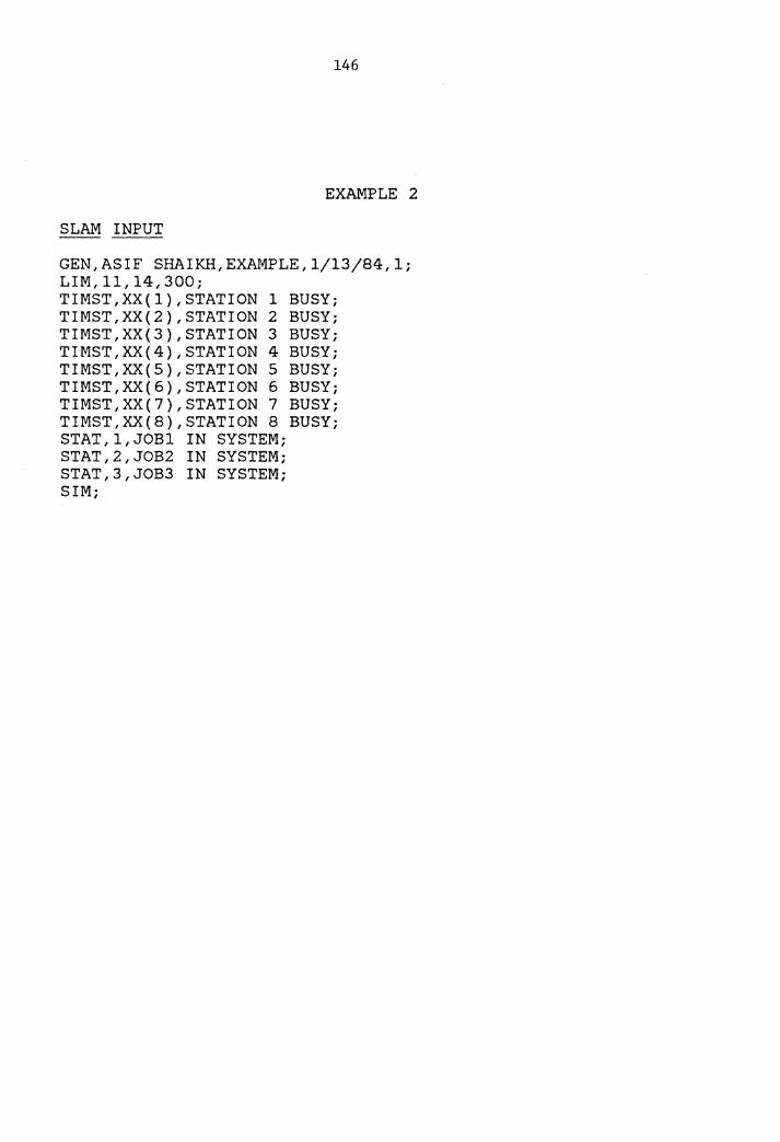
146
EXAMPLE 2
SLAM INPUT
GEN,ASIF SHAIKH,EXAMPLE,1/13/84,l; LIM,11,14,300; TIMST,XX(l},STATION 1 BUSY; TIMST,XX(2),STATION 2 BUSY; TIMST,XX(3),STATION 3 BUSY; TIMST,XX(4),STATION 4 BUSY; TIMST,XX(S},STATION 5 BUSY; TIMST,XX(6),STATION 6 BUSY; TIMST,XX(7),STATION 7 BUSY; TIMST,XX(8),STATION 8 BUSY; STAT,l,JOBl IN SYSTEM; STAT,2,JOB2 IN SYSTEM; STAT,3,JOB3 IN SYSTEM; SIM;

. 147
MODEL INPUT 2 0 9 0 0 0 0 1 2 0 0 1 1 0 0 3 3 4 5 1 2 0 0 1 6 0 0 1 2 0 0 2 6 7 0 1 2 0 0 1 8 0 0 2 3 4 0 1 9 0 0 1 4 0 0 1 9 0 0 1 5 0 0 1 9 0 0 3 6 7 8 0 0 0 0 11 5. 3. 4. 6. 3. 5. 4. 4. 3. 3. 3. 1 2 2 3 2 4 2 5 3 6 4 6 4 7 5 8 6 9 7 9 8 9 5. 1. 5 8 1 1 1 1 2 1 1 2 1 0. 1 5. 1 10. 1 7.7 1 12. 1 10.5 1 8.5 1 0. 1 1 0 0 0 0 1 0 0 0 0 1 2 0 0 0 0 1 0 0 0 0 1 3 0 0 0 0 1 0 0 0 0
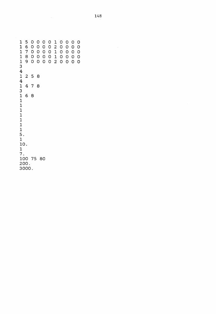
148
1 5 0 0 0 0 1 0 0 0 0 1 6 0 0 0 0 2 0 0 0 0 1 7 0 0 0 0 1 0 0 0 0 1 8 0 0 0 0 1 0 0 0 0 1 9 0 0 0 0 2 0 0 0 0 3 4 1 2 5 8 4 1 4 7 8 3 1 6 8 1 1 1 1 1 1 1 5. 1 10. 1 7. 100 75 80 200. 3000.
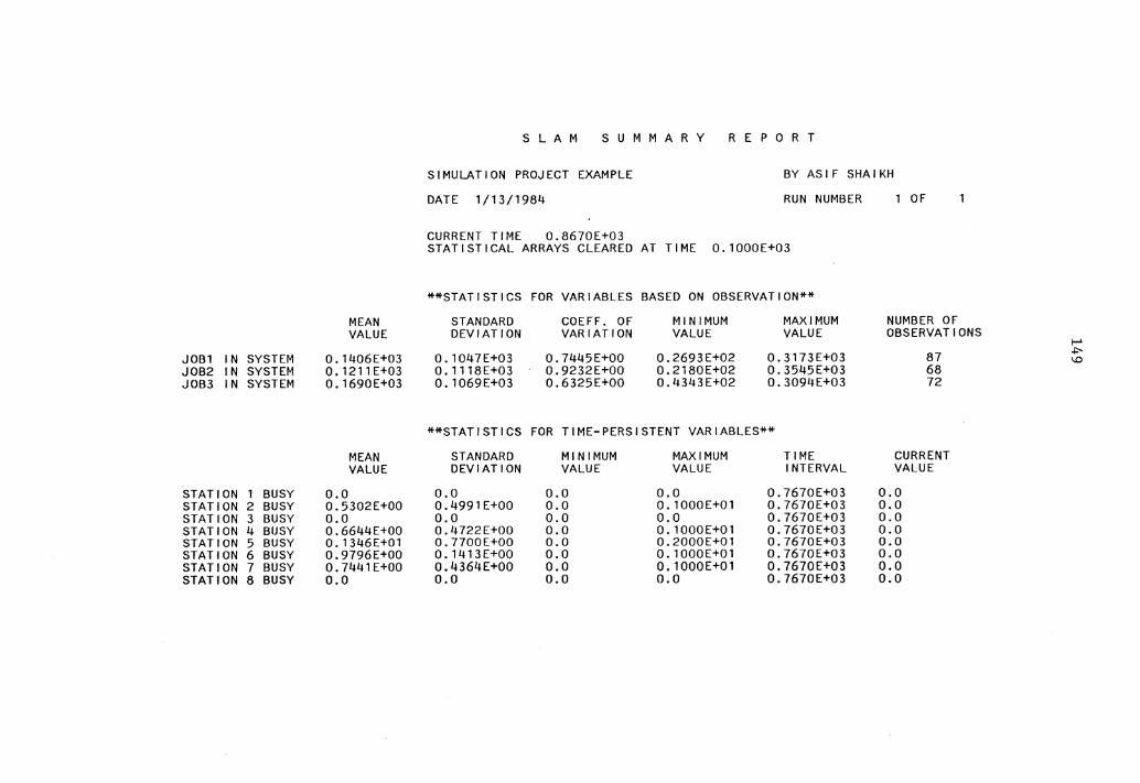
S L A M S U M M A R Y R E P 0 R T
SIMULATION PROJECT EXAMPLE BY ASIF SHAIKH
DATE 1/13/1984 RUN NUMBER OF
CURRENT TIME 0.8670E+03 STATISTICAL ARRAYS CLEARED AT TIME O. 1000E+03
**STATISTICS FOR VARIABLES BASED ON OBSERVATION**
MEAN STANDARD COEFF. OF MINIMUM MAXIMUM NUMBER OF VALUE DEVIATION VARIATION VALUE VALUE OBSERVATIONS .....
JOBl IN SYSTEM 0. l 406E+03 0.1047E+03 0.7445E+OO 0.2693E+02 0. 3173E+03 87 ~ ~
JOB2 IN SYSTEM 0.1211E+03 0.1118E+03 0.9232E+OO 0.2180E+02 0.3545E+03 68 JOB3 IN SYSTEM 0. 1690E+03 0. 1069E+03 0.6325E+OO 0.4343E+02 0.3094E+03 72
**STATISTICS FOR TIME-PERSISTENT VARIABLES**
MEAN STANDARD MINIMUM MAXIMUM TIME CURRENT VALUE DEVIATION VALUE VALUE INTERVAL VALUE
STATION 1 BUSY 0.0 0.0 o.o 0.0 0.7670E+03 0.0 STATION 2 BUSY 0.5302E+OO 0.4991E+OO 0.0 O. lOOOE+Ol 0.7670E+03 0.0 STATION 3 BUSY 0.0 0.0 0.0 0.0 0.7670E+03 0.0 STATION 4 BUSY 0.6644E+OO 0.4722E+OO 0.0 0. lOOOE+Ol 0.7670E+03 0.0 STAT! ON 5 BUSY 0. 1346E+01 0.7700E+OO 0.0 0.2000E+01 0.7670E+03 0.0 STATION 6 BUSY 0.9796E+OO 0.1413E+OO 0.0 O.lOOOE+Ol 0.7670E+03 0.0 STATION 7 BUSY 0.7441E+OO 0.4364E+OO 0.0 O.lOOOE+Ol 0.7670E+03 0.0 STATION 8 BUSY 0.0 0.0 0.0 0.0 0.7670E+03 0.0
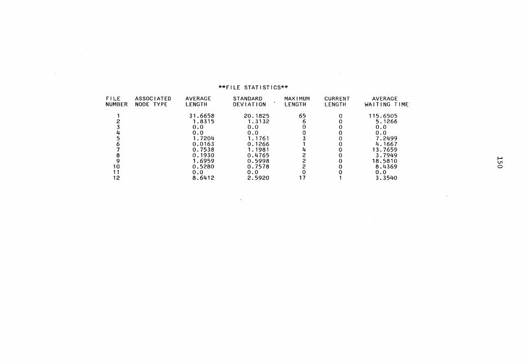
**FILE STATISTICS** FILE ASSOCIATED AVERAGE STANDARD MAXIMUM CURRENT AVERAGE NUMBER NODE TYPE LENGTH DEVIATION LENGTH LENGTH WAITING TIME
1 31.6658 20. 1825 65 0 115.6505 2 1.8315 1.3132 6 0 5. 1266 3 0.0 0.0 0 0 0.0 4 o.o o.o 0 0 0.0 5 1.7204 1.1761 3 0 7.2499 6 0.0163 0. 1266 1 0 4.1667 7 0.7538 1.1981 4 0 13.7659 8 0.1930 0.4765 2 0 3.7949 }-I 9 1.6959 0.5998 2 0 18.5810 Vt
10 0.5280 0.7578 2 0 8.4369 0 11 0.0 0.0 0 0 o.o 12 8.6412 2.5920 17 1 3.3540
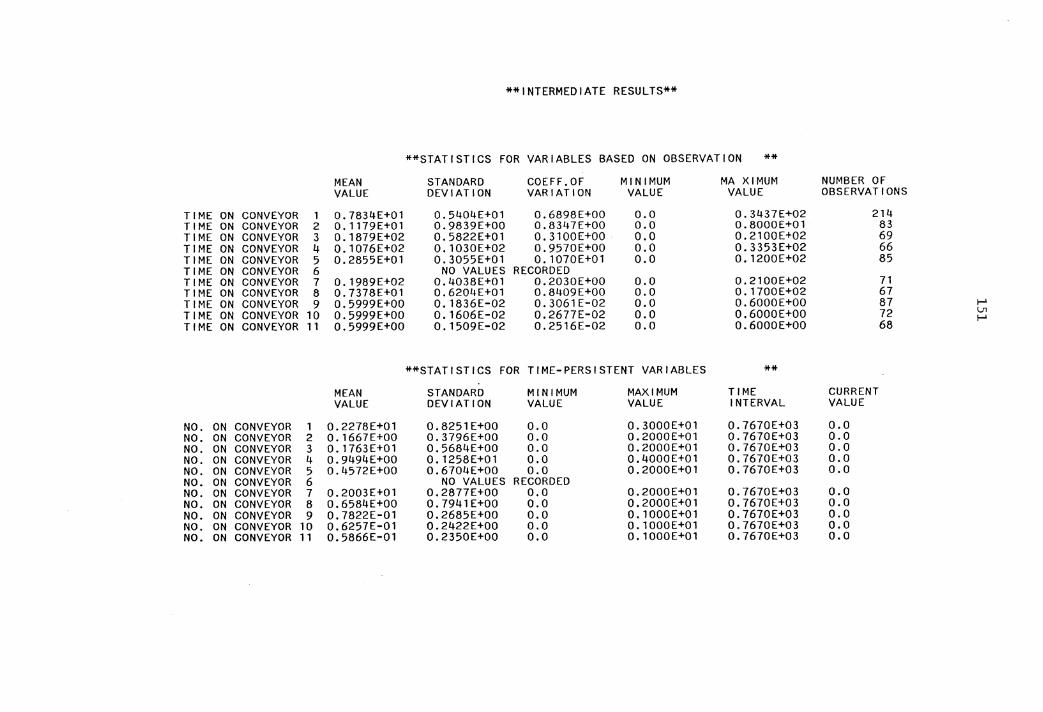
**INTERMEDIATE RESULTS**
**STATISTICS FOR VARIABLES BASED ON OBSERVATION **
MEAN STANDARD COEFF. OF MINIMUM MA XIMUM NUMBER OF VALUE DEVIATION VARIATION VALUE VALUE OBSERVATIONS
TIME ON CONVEYOR 1 0.7834E+01 0.5404E+01 0.6898E+OO o.o 0.3437E+02 214 TIME ON CONVEYOR 2 0.1179E+01 0.9839E+OO 0.8347E+OO o.o 0.8000E+01 83 TIME ON CONVEYOR 3 O. 1879E+02 0.5822E+01 0.3100E+OO o.o 0.2100E+02 69 TIME ON CONVEYOR 4 0. 1076E+02 0. 1030E+02 0.9570E+OO 0.0 0.3353E+02 66 TIME ON CONVEYOR 5 0.2855E+01 0.3055E+01 0.1070E+01 o.o 0.1200E+02 85 TIME ON CONVEYOR 6 NO VALUES RECORDED TIME ON CONVEYOR 7 0.1989E+02 0.4038E+01 0.2030E+OO 0.0 0.2100E+02 71 TIME ON CONVEYOR 8 0.7378E+01 0.6204E+01 0.8409E+OO 0.0 0.1700E+02 67 TIME ON CONVEYOR 9 0.5999E+OO 0.1836E-02 0.3061E-02 0.0 0.6000E+OO 87 l-' TIME ON CONVEYOR 10 0.5999E+OO 0.1606E-02 0.2677E-02 0.0 0.6000E+OO 72 Vl
TIME ON CONVEYOR 11 0.5999E+OO 0. 1509E-02 0.2516E-02 0.0 0.6000E+OO 68 I-'
**STATISTICS FOR TIME-PERSISTENT VARIABLES **
MEAN STANDARD MINIMUM MAXIMUM TIME CURRENT VALUE DEVIATION VALUE VALUE INTERVAL VALUE
NO. ON CONVEYOR 1 0.2278£+01 0.8251E+OO o.o 0.3000E+01 0.7670E+03 0.0 NO. ON CONVEYOR 2 0.1667E+OO 0.3796E+OO o.o 0.2000E+01 0.7670E+03 0.0 NO. ON CONVEYOR 3 0.1763E+01 0.5684E+OO 0.0 0.200QE+01 0.7670E+03 0.0 NO. ON CONVEYOR 4 0.9494E+OO 0. 1258E+01 o.o 0.4000E+01 0.7670E+03 0.0 NO. ON CONVEYOR 5 0.4572E+OO 0.6704E+OO 0.0 0.2000E+01 0.7670E+03 o.o NO. ON CONVEYOR 6 NO VALUES RECORDED NO. ON CONVEYOR 7 0.2003E+01 0.2877E+OO 0.0 0.2000E+01 0.7670E+03 o.o NO. ON CONVEYOR 8 0.6584E+OO 0.7941E+OO 0.0 0.2000E+01 0.7670E+03 o.o NO. ON CONVEYOR 9 0.7822E-01 0.2685E+OO o.o 0. 1000E+01 0.7670E+03 0.0 NO. ON CONVEYOR 10 0.6257E-01 0.2422£+00 o.o O. 1000£+01 0.7670E+03 o.o NO. ON CONVEYOR 11 0.5866E-01 0.2350E+OO o.o O. lOOOE+Ol 0.7670£+03 o.o
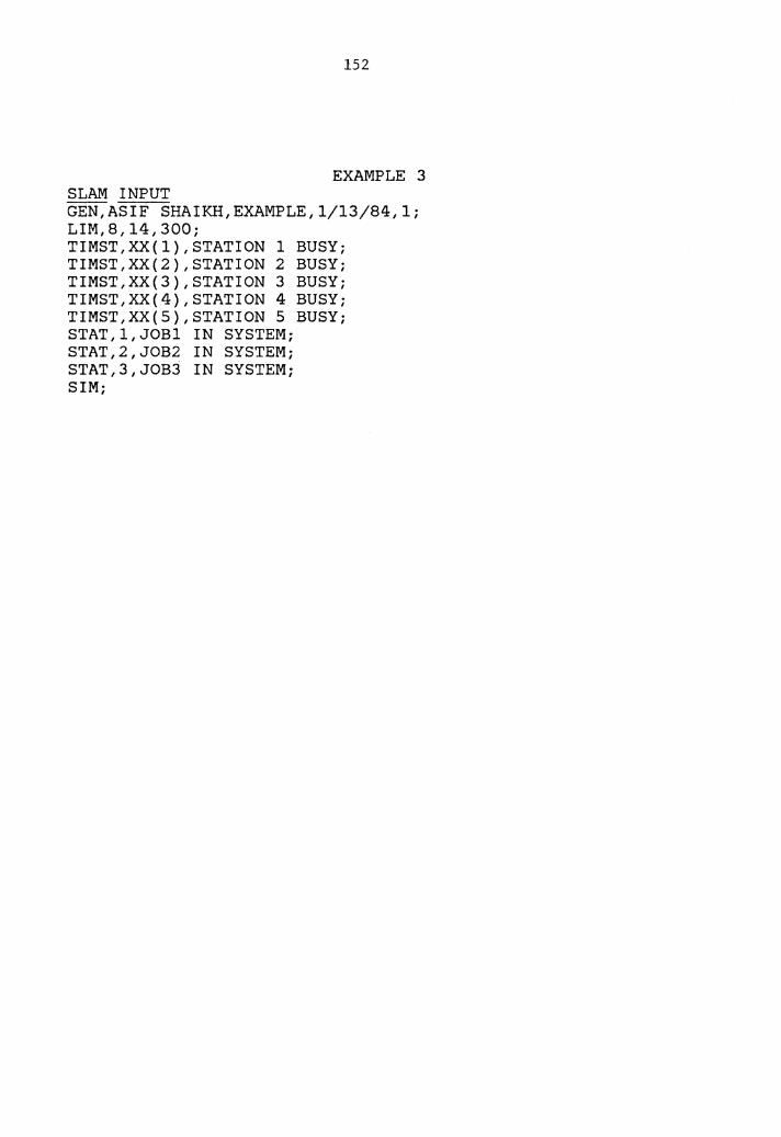
152
EXAMPLE 3 SLAM INPUT GEN,ASIF SHAIKH,EXAMPLE,1/13/84,l; LIM,8,14,300; TIMST,XX(l),STATION 1 BUSY; TIMST,XX(2),STATION 2 BUSY; TIMST,XX(3),STATION 3 BUSY; TIMST,XX(4),STATION 4 BUSY; TIMST,XX(S),STATION 5 BUSY; STAT,l,JOBl IN SYSTEM; STAT,2,JOB2 IN SYSTEM; STAT,3,JOB3 IN SYSTEM; SIM;
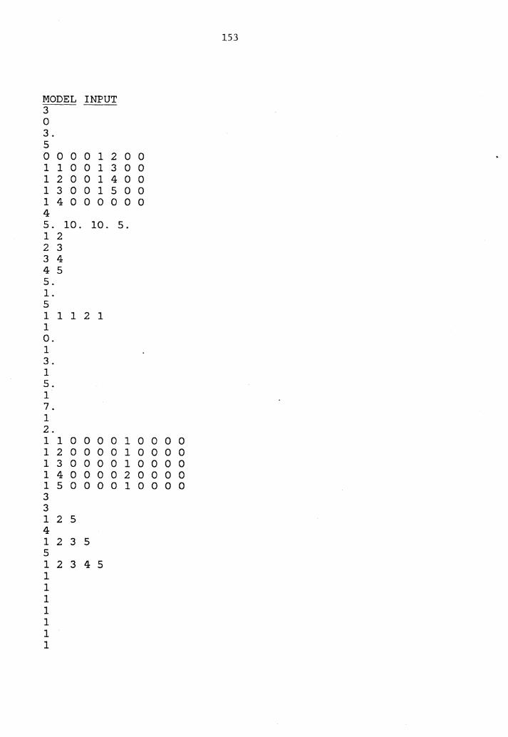
153
MODEL INPUT 3 0 3. 5 0 0 0 0 1 2 0 0 1 1 0 0 1 3 0 0 1 2 0 0 1 4 0 0 1 3 0 0 1 5 0 0 1 4 0 0 0 0 0 0 4 5. 10. 10. 5. 1 2 2 3 3 4 4 5 5. 1. 5 1 1 1 2 1 1 0. 1 3. 1 5. 1 7. 1 2. 1 1 0 0 0 0 1 0 0 0 0 1 2 0 0 0 0 1 0 0 0 0 1 3 0 0 0 0 1 0 0 0 0 1 4 0 0 0 0 2 0 0 0 0 1 5 0 0 0 0 1 0 0 0 0 3 3 1 2 5 4 1 2 3 5 5 1 2 3 4 5 1 1 1 1 1 1 1
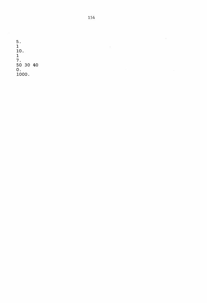
5. 1 10. 1 7. 50 30 40 0. 1000.
154
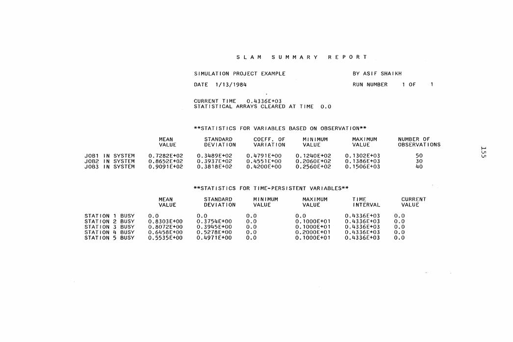
MEAN VALUE
JO Bl IN SYSTEM 0.7282E+02 JOB2 IN SYSTEM 0.8652E+02 JOB3 IN SYSTEM 0.9091E+02
MEAN VALUE
STATION 1 BUSY 0.0 STATION 2 BUSY 0.8303E+OO STATION 3 BUSY 0.8072E+OO STATION 4 BUSY 0.6458E+OO STATION 5 BUSY 0.5535E+OO
S L A M S U M M A R Y R E P 0 R T
SIMULATION PROJECT EXAMPLE
DATE 1 /13/1984
BY ASIF SHAIKH
RUN NUMBER OF
CURRENT TIME 0.4336E+03 STATISTICAL ARRAYS CLEARED AT TIME 0.0
**STATISTICS FOR VARIABLES BASED ON OBSERVATION**
STANDARD COEFF. OF MINIMUM MAXIMUM NUMBER OF DEVIATION VARIATION VALUE VALUE OBSERVATIONS
0.3489E+02 0.4791E+OO 0.1240E+02 0.1302E+03 50 0.3937E+02 0.4551E+OO 0.2060E+02 0.1386E+03 30 0.3818E+02 0.4200E+OO 0.2560E+02 0.1506E+03 40
**STATISTICS FOR TIME-PERSISTENT VARIABLES**
STANDARD MINIMUM MAXIMUM TIME CURRENT DEVIATION VALUE VALUE INTERVAL VALUE
0.0 0.0 0.0 0.4336E+03 0.0 0.3754E+OO 0.0 0. lOOOE+Ol 0.4336E+03 o.o 0.3945E+OO 0.0 O.lOOOE+Ol 0.4336E+03 0.0 0.5278E+OO 0.0 0.2000E+01 0.4336E+03 0.0 0.4971E+OO 0.0 0. lOOOE+Ol 0.4336E+03 0.0
1-' \.J1 \.J1
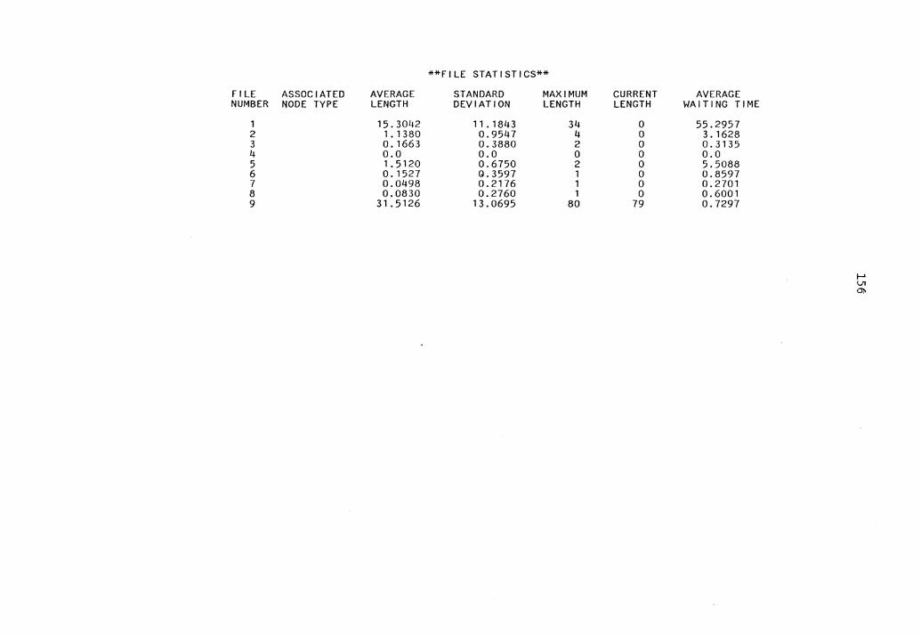
FILE ASSOCIATED AVERAGE NUMBER NODE TYPE LENGTH
1 15.3042 2 1 . 1 380 3 0.1663 4 0.0 5 1.5120 6 0. 1527 7 0.0498 8 0.0830 9 31.5126
**FILE STATISTICS**
STANDARD MAXIMUM DEVIATION LENGTH
11.1843 34 0.9547 4 0.3880 2 0.0 0 0.6750 2 Q.3597 1 0.2176 1 0.2760 1
13.0695 80
CURRENT LENGTH
0 0 0 0 0 0 0 0
79
AVERAGE WAITING TIME
55.2957 3. 1628 0.3135 0.0 5.5088 0.8597 0.2701 0.6001 0.7297
~ Ul <»
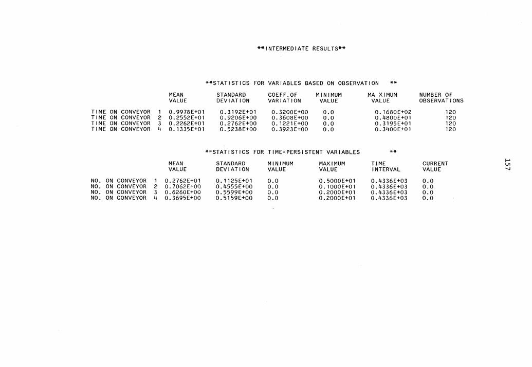
**INTERMEDIATE RESULTS**
**STATISTICS FOR VARIABLES BASED ON OBSERVATION **
MEAN STANDARD COEFF.OF MINIMUM MA XIMUM NUMBER OF VALUE DEVIATION VARIATION VALUE VALUE OBSERVATIONS
TIME ON CONVEYOR 1 0.9978E+01 0.3192E+01 0.3200E+OO o.o 0. 1680E+02 120 TIME ON CONVEYOR 2 0.2552E+01 0.9206E+OO 0.3608E+OO 0.0 0.4800E+01 120 TIME ON CONVEYOR 3 0.2262E+Ol 0.2762E+OO 0.1221E+OO 0.0 0.3195E+Ol 120 TIME ON CONVEYOR 4 0.1335E+01 0.5238E+OO O. 3923E+OO 0.0 0.3400E+01 120
**STATISTICS FOR TIME-PERSISTENT VARIABLES **
MEAN STANDARD MINIMUM MAXIMUM TIME CURRENT f--' ln
VALUE DEVIATION VALUE VALUE INTERVAL VALUE -...J
NO. ON CONVEYOR 1 0.2762E+01 0.1125E+01 0.0 0.5000E+01 0.4336E+03 0.0 NO. ON CONVEYOR 2 0.7062E+OO 0.4555E+OO 0.0 0.1000E+Ol 0.4336E+03 0.0 NO. ON CONVEYOR 3 0.6260E+OO 0.5599E+OO 0.0 0.2000E+01 0.4336E+03 0.0 NO. ON CONVEYOR 4 0.3695E+OO 0.5159E+OO 0.0 0.2000E+01 0.4336E+03 0.0
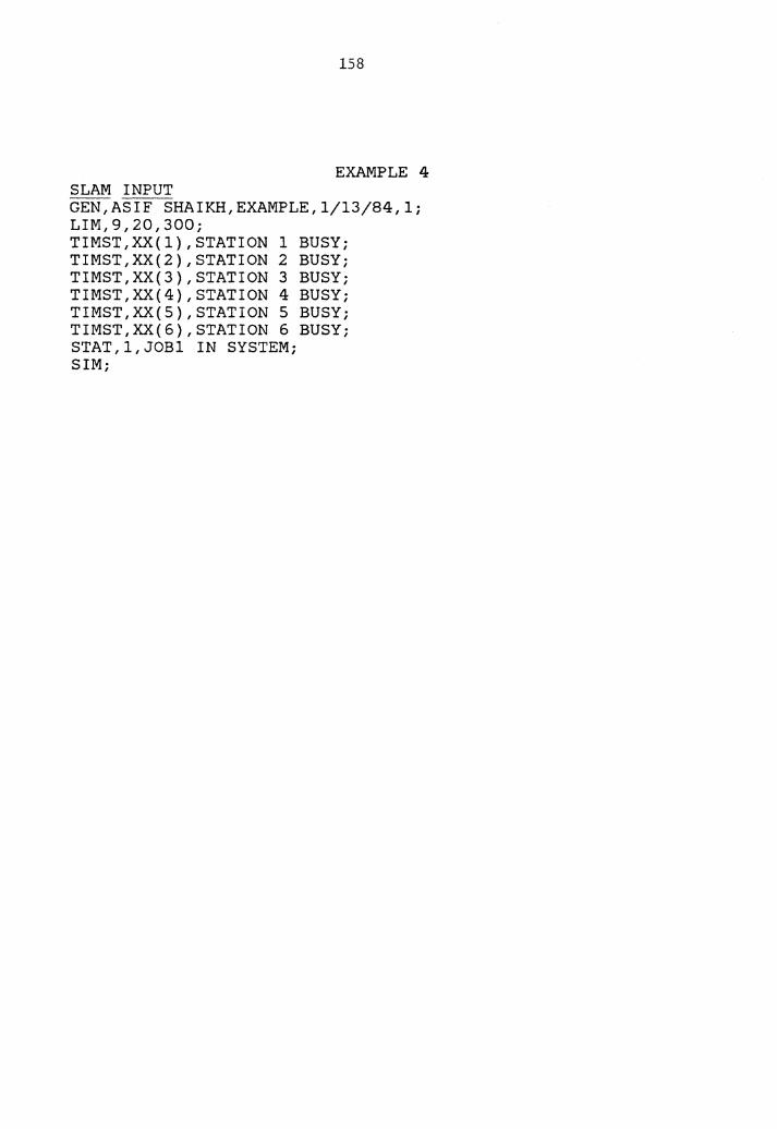
158
EXAMPLE 4 SLAM INPUT GEN,ASIF SHAIKH,EXAMPLE,1/13/84,l; LIM,9,20,300; TIMST,XX(l},STATION 1 BUSY; TIMST,XX(2},STATION 2 BUSY; TIMST,XX(3},STATION 3 BUSY; TIMST,XX(4},STATION 4 BUSY; TIMST,XX(S},STATION 5 BUSY; TIMST,XX(6},STATION 6 BUSY; STAT,l,JOBl IN SYSTEM; SIM;
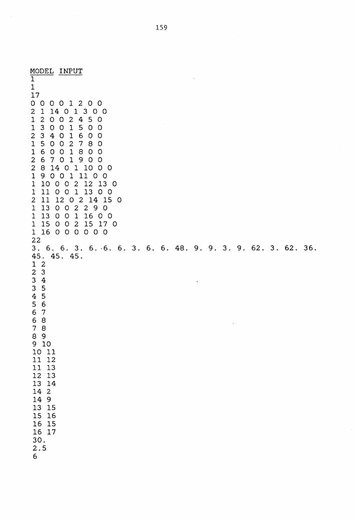
MODEL INPUT 1 1 17 0 0 0 0 1 2 0 0 2 1 14 0 1 3 0 0 1 2 0 0 2 4 5 0 1 3 0 0 1 5 0 0 2 3 4 0 1 6 0 0 1 5 0 0 2 7 8 0 1 6 0 0 1 8 0 0 2 6 7 0 1 9 0 0 2 8 14 0 1 10 0 0 1 9 0 0 1 11 0 0 1 10 0 0 2 12 13 0 1 11 0 0 1 13 0 0 2 11 12 0 2 14 15 0 1 13 0 0 2 2 9 0 1 13 0 0 1 16 0 0 1 15 0 0 2 15 17 0 1 16 0 0 0 0 0 0 22
159
3 . 6 . 6 . 3 . 6 . . 6 . 6 . 3 . 6 . 6 . 48 . 9 . 9 . 3 . 9 . 62 . 3 . 62 . 3 6. 45. 45. 45. 1 2 2 3 3 4 3 5 4 5 5 6 6 7 6 8 7 8 8 9 9 10 10 11 11 12 11 13 12 13 13 14 14 2 14 9 13 15 15 16 16 15 16 17 30. 2.5 6
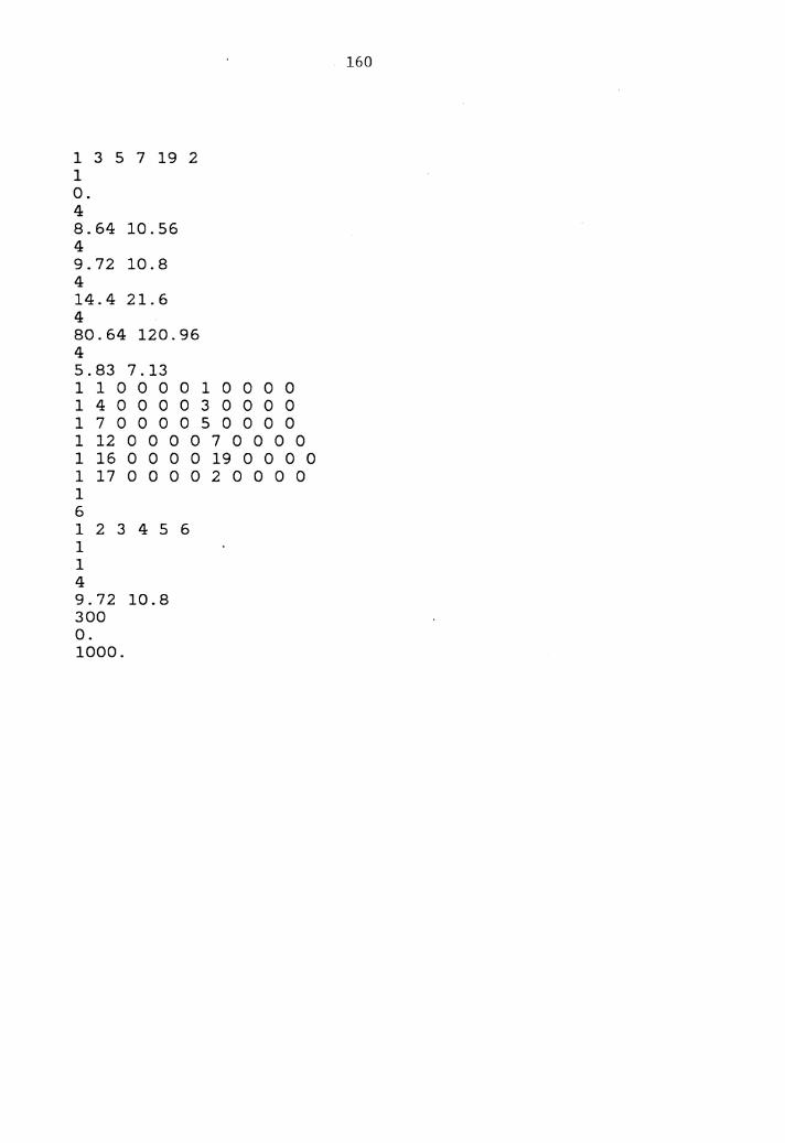
1 3 5 7 19 2 1 0. 4 8.64 10.56 4 9.72 10.8 4 14.4 21.6 4 80.64 120.96 4 5.83 7.13 1 1 0 0 0 0 1 0 0 0 0 1 4 0 0 0 0 3 0 0 0 0 1 7 0 0 0 0 5 0 0 0 0 1 12 0 0 0 0 7 0 0 0 0 1 16 0 0 0 0 19 0 0 0 0 1 17 0 0 0 0 2 0 0 0 0 1 6 1 2 3 4 5 6 1 1 4 9.72 10.8 300 0. 1000.
160

Run 1
**STATISTICS FOR VARIABLES BASED ON OBSERVATION **
MEAN STANDARD COE FF. OF MINIMUM MA XIMUM NUMBER OF VALUE DEVIATION VARIATION VALUE VALUE OBSERVATIONS
T ME ON CONVEYOR 1 0.9989E-01 0.3524E-04 0.3528E-03 o.o O.lOOOE+OO 97 T ME ON CONVEYOR 2 0.2000E+OO 0.6063E-03 0.3032E-02 0.0 0.2000E+OO 97 T ME ON CONVEYOR 3 0.2000E+OO 0.6063E-03 0.3032E-02 0.0 0.2000E+OO 97 T ME ON CONVEYOR 4 NO VALUES RECORDED T ME ON CONVEYOR 5 0.2000E+OO 0.6176E-03 0.3089E-02 0.0 0.2000E+OO 96 T ME ON CONVEYOR 6 0.2000E+OO 0.6176E-03 0.3089E-02 0.0 0.2000E+OO 96 T ME ON CONVEYOR 7 o.2000E+oo 0.6176E-03 0.3089E-02 o.o 0.2000E+OO 96 }--' T ME ON CONVEYOR 8 NO VALUES RECORDED °' T ME ON CONVEYOR 9 0.2000E+OO 0.6127E-03 0.3064E-02 0.0 0.2000E+OO 95 ...... T ME ON CONVEYOR 10 0.2000E+OO 0.6127E-03 0.3064E-02 o.o 0.2000E+OO 95 T ME ON CONVEYOR 11 0.1600E+01 0.2417E-02 0.1511E-02 0.0 0.1600E+01 95 T ME ON CONVEYOR 12 0.2998E+OO o.o o.o o.o 0.3000E+OO 95 T ME ON CONVEYOR 13 0.2998E+OO 0.0 0.0 o.o 0.3000E+OO 95 T ME ON CONVEYOR 14 NO VALUES RECORDED TIME ON CONVEYOR 15 0.2998E+OO 0.0 0.0 o.o 0.3000E+OO 93 TIME ON CONVEYOR 16 NO VALUES RECORDED TIME ON CONVEYOR 17 NO VALUES RECORDED TIME ON CONVEYOR 18 NO VALUES RECORDED TIME ON CONVEYOR 19 0. 1200E+01 O. 1468E-02 0.1224E-02 o.o O. 1200E+01 93 TIME ON CONVEYOR 20 O. 1500E+01 0.0 0.0 0.0 0.1500E+01 93 TIME ON CONVEYOR 21 NO VALUES RECORDED TIME ON CONVEYOR 22 0.1660E+01 0.5949E+OO 0.3584E+OO 0.0 0.4439E+01 82
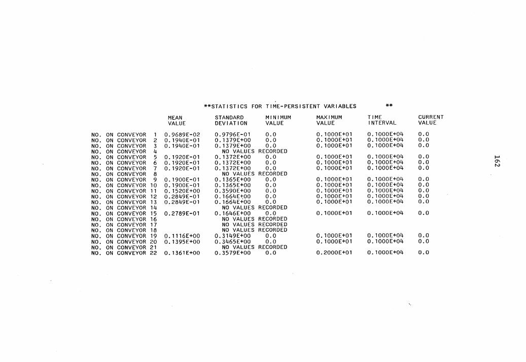
**STATISTICS FOR TIME-PERSISTENT VARIABLES **
MEAN STANDARD MINIMUM MAXIMUM TIME CURRENT VALUE DEVIATION VALUE VALUE INTERVAL VALUE
NO. ON CONVEYOR 1 0.9689E-02 0.9796E-Ol 0.0 0. lOOOE+Ol O. 1000E+04 0.0 NO. ON CONVEYOR 2 0.1940E-Ol 0.1379E+OO 0.0 O.lOOOE+Ol 0.1000E+04 0.0 NO. ON CONVEYOR 3 0.1940E-Ol 0.1379E+OO 0.0 0. lOOOE+Ol O. 1000E+04 0.0 NO. ON CONVEYOR 4 NO VALUES RECORDED NO. ON CONVEYOR 5 0.1920E-Ol 0.1372E+OO 0.0 O. lOOOE+Ol 0.1000E+04 o.o ....... NO. ON CONVEYOR 6 0.1920E-01 0.1372E+OO 0.0 O.lOOOE+Ol 0.1000E+04 0.0 "' NO. ON CONVEYOR 7 0.1920E-Ol 0.1372E+OO 0.0 O.lOOOE+Ol 0.1000E+04 0.0 N
NO. ON CONVEYOR 8 NO VALUES RECORDED NO. ON CONVEYOR 9 0.1900E-Ol 0.1365E+OO 0.0 0. lOOOE+Ol 0. 1000E+04 o.o NO. ON CONVEYOR 10 0.1900E-01 o. 1365E+oo 0.0 O.lOOOE+Ol 0.1000E+04 o.o NO. ON CONVEYOR 11 0.1520E+OO 0.3590E+OO 0.0 O.lOOOE+Ol 0. 1000E+04 0.0 NO. ON CONVEYOR 12 0.2849E-Ol 0. 1664E1;00 0.0 0. lOOOE+Ol 0. 1 OOOE+04 0.0 NO. ON CONVEYOR 13 0.2849E-Ol 0.1664E+OO 0.0 O. lOOOE+Ol 0. 1000E+04 0.0 NO. ON CONVEYOR 14 NO VALUES RECORDED NO. ON CONVEYOR 15 0.2789E-Ol 0.1646E+OO 0.0 0. lOOOE+Ol 0.1000E+04 0.0 NO. ON CONVEYOR 16 NO VALUES RECORDED NO. ON CONVEYOR 17 NO VALUES RECORDED NO. ON CONVEYOR 18 NO VALUES RECORDED NO. ON CONVEYOR 19 0.1116E+OO 0.3149E+OO 0.0 0. 1000E+01 0.1000E+04 0.0 NO. ON CONVEYOR 20 0.1395E+OO o.3465E+oo 0.0 0. lOOOE+Ol 0. 1000E+04 0.0 NO. ON CONVEYOR 21 NO VALUES RECORDED NO. ON CONVEYOR 22 0.1361E+OO 0.3579E+OO 0.0 0.2000E+Ol 0.1000E+04 o.o
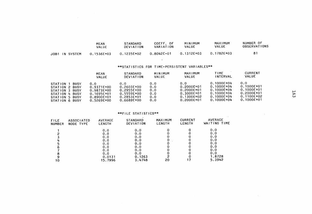
MEAN STANDARD COE FF. OF MINIMUM MAXIMUM NUMBER OF VALUE DEVIATION VARIATION VALUE VALUE OBSERVATIONS
JOBl IN SYSTEM 0.1536E+03 0. 1235E+02 0.8042E-Ol 0. 13 l 2E+03 0.1782E+03 81
**STATISTICS FOR TIME-PERSISTENT VARIABLES**
MEAN STANDARD MINIMUM MAXIMUM TIME CURRENT VALUE DEVIATION VALUE VALUE INTERVAL VALUE
STATION 1 BUSY 0.0 0.0 0.0 0.0 0.1000E+04 0.0 STATION 2 BUSY 0.9371E+OO 0.2603E+OO 0.0 0.2000E+Ol 0.1000E+04 O.lOOOE+Ol STATION 3 BUSY 0.9873E+OO 0.2955E+OO 0.0 0.2000E+Ol 0.1000E+04 0. lOOOE+Ol STATION 4 BUSY 0. 1695E+Ol 0.5559E+OO 0.0 0.3000E+Ol 0. 1000E+04 0.2000E+Ol !--"
°' STATION 5 BUSY 0.8900E+Ol 0.2853E+Ol 0.0 0. 1300E+02 0. 1000E+04 0.1100E+02 (,...)
STATION 6 BUSY 0.5269E+OO 0.6689E+OO o.o 0.2000E+Ol 0.1000E+04 0. lOOOE+Ol
**FILE STATISTICS**
FILE ASSOCIATED AVERAGE STANDARD MAXIMUM CURRENT AVERAGE NUMBER NODE TYPE LENGTH DEVIATION LENGTH LENGTH WAITING TIME
1 o.o 0.0 0 0 0.0 2 0.0 0.0 0 0 0.0 3 0.0 0.0 0 0 0.0 4 0.0 0.0 0 0 0.0 5 o.o 0.0 0 0 0.0 6 0.0 o.o 0 0 0.0 7 0.0 0.0 0 0 0.0 8 0.0 0.0 0 0 0.0 9 0.0131 0. 1263 2 0 1. 8728
10 15.7996 3.4748 20 17 5.3942
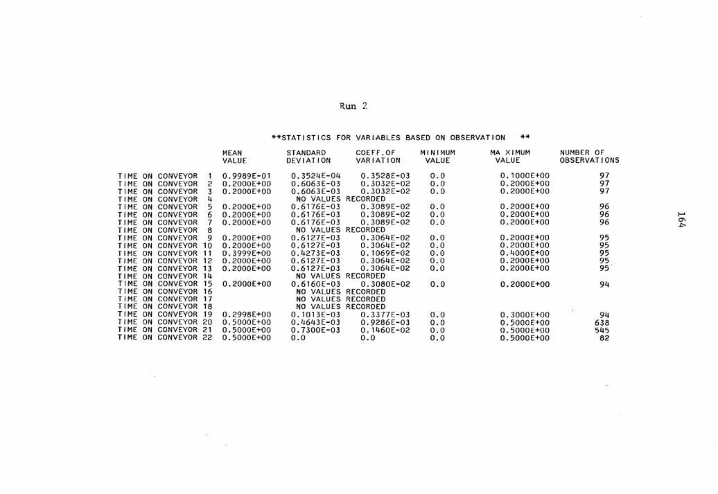
Run 2.
**STATISTICS FOR VARIABLES BASED ON OBSERVATION **
MEAN STANDARD COE FF. OF MINIMUM MA XIMUM NUMBER OF VALUE DEVIATION VARIATION VALUE VALUE OBSERVATIONS
T ME ON CONVEYOR 1 0.9989E-01 0.3524E-04 0.3528E-03 0.0 O.lOOOE+OO 97 T ME ON CONVEYOR 2 0.2000E+OO 0.6063E-03 0.3032E-02 0.0 0.2000E+OO 97 T ME ON CONVEYOR 3 0.2000E+OO 0.6063E-03 0.3032E-02 o.o 0.2000E+OO 97 T ME ON CONVEYOR 4 NO VALUES RECORDED T ME ON CONVEYOR 5 0.2000E+OO 0.6176E-03 0.3089E-02 o.o 0.2000E+OO 96 T ME ON CONVEYOR 6 0.2000E+OO 0.6176E-03 0.3089E-02 0.0 0.2000E+OO 96 ....... T ME ON CONVEYOR 7 0.2000E+OO 0.6176E-03 0.3089E-02 0.0 0.2000E+OO 96 °' -1:'-T ME ON CONVEYOR 8 NO VALUES RECORDED T ME ON CONVEYOR 9 0.2000E+OO 0.6127E-03 0.3064E-02 0.0 0.2000E+OO 95 T ME ON CONVEYOR 10 0.2000E+OO 0.6127E-03 0.3064E-02 0.0 0.2000E+OO 95 T ME ON CONVEYOR 11 0.3999E+OO 0.4273E-03 0. 1069E-02 o.o 0.4000E+OO 95 T ME ON CONVEYOR 12 0.2000E+OO 0.6127E-03 0.3064E-02 0.0 0.2000E+OO 95 T ME ON CONVEYOR 13 0.2000E+OO 0.6127E-D3 0.3064E-02 0.0 0.2000E+OO 95 T ME ON CONVEYOR 14 NO VALUES RECORDED T ME ON CONVEYOR 15 0.2000E+OO 0.6160E-03 0.3080E-02 0.0 0.2000E+OO 94 TIME ON CONVEYOR 16 NO VALUES RECORDED TIME ON CONVEYOR 17 NO VALUES RECORDED TIME ON CONVEYOR 18 NO VALUES RECORDED TIME ON CONVEYOR 19 0.2998E+OO 0.1013E-03 0. 3377E-03 0.0 0.3000E+OO 94 TIME ON CONVEYOR 20 0.5000E+OO 0.4643E-03 0.9286E-03 0.0 0.5000E+OO 638 TIME ON CONVEYOR 21 0.5000E+OO 0.7300E-03 0.1460E-02 0.0 0.5000E+OO 545 TIME ON CONVEYOR 22 0.5000E+OO o.o o.o 0.0 0.5000E+OO 82
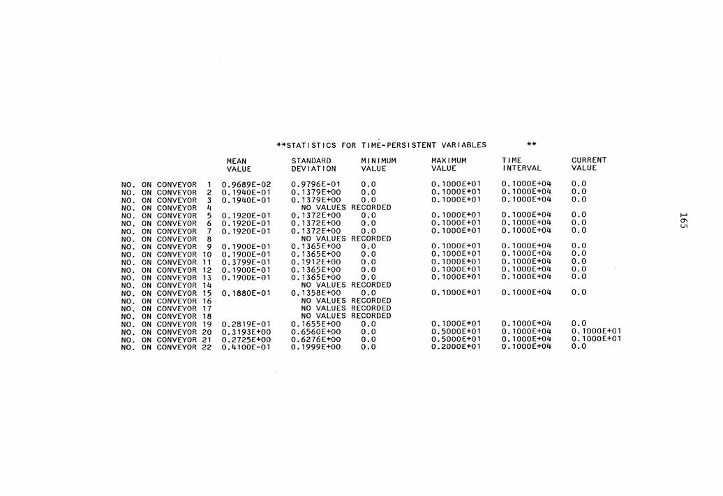
**STATISTICS FOR TIME-PERSISTENT VARIABLES **
MEAN STANDARD MINIMUM MAXIMUM TIME CURRENT VALUE DEVIATION VALUE VALUE INTERVAL VALUE
NO. ON CONVEYOR 1 0.9689E-02 0.9796E-Ol 0.0 0. lOOOE+Ol 0.1000E+04 0.0 NO. ON CONVEYOR 2 0. 1940E-Ol 0.1379E+OO 0.0 0.1000E+01 0. 1000E+04 0.0 NO. ON CONVEYOR 3 0.1940E-Ol 0.1379E+OO 0.0 O.lOOOE+Ol 0.1000E+04 0.0 NO. ON CONVEYOR 4 NO VALUES RECORDED NO. ON CONVEYOR 5 0. 1920E-Ol 0.1372E+OO 0.0 O. lOOOE+Ol 0.1000E+04 0.0 ...... NO. ON CONVEYOR 6 0.1920E-Ol 0.1372E+OO 0.0 O. lOOOE+Ol 0. 1 OOOE+04 0.0 °' NO. ON CONVEYOR 7 O. 1920E-01 0.1372E+OO 0.0 O. lOOOE+Ol 0. 1000E+04 0.0 Vl
NO. ON CONVEYOR 8 NO VALUES RECORDED NO. ON CONVEYOR 9 0.1900E-Ol 0.1365E+OO 0.0 O. lOOOE+Ol 0. 1000E+04 0.0 NO. ON CONVEYOR 10 0.1900E-Ol 0.1365E+OO 0.0 O.lOOOE+Ol O. 1000E+04 o.o NO. ON CONVEYOR 11 0.3799E-Ol 0.1912E+OO 0.0 0.1000E+01 0.1000E+04 0.0 NO. ON CONVEYOR 12 0.1900E-Ol 0.1365E+OO 0.0 O.lOOOE+Ol 0.1000E+04 0.0 NO. ON CONVEYOR 13 0.1900E-Ol 0.1365E+OO 0.0 O.lOOOE+Ol 0.1000E+04 0.0 NO. ON CONVEYOR 14 NO VALUES RECORDED NO. ON CONVEYOR 15 0.1880E-Ol 0.1358E+OO 0.0 O.lOOOE+Ol 0.1000E+04 0.0 NO. ON CONVEYOR 16 NO VALUES RECORDED NO. ON CONVEYOR 17 NO VALUES RECORDED NO. ON CONVEYOR 18 NO VALUES RECORDED NO. ON CONVEYOR 19 0.2819E-01 0.1655E+OO 0.0 0.1000E+01 0.1000E+04 0.0 NO. ON CONVEYOR 20 0.3193E+OO 0.6560E+OO 0.0 0.5000E+Ol O. 1000E+04 O. lOOOE+Ol NO. ON CONVEYOR 21 o.2125E+oo o.6276E+oo 0.0 0.5000E+Ol O. 1000E+04 0. 1 OOOE+Ol NO. ON CONVEYOR 22 0.4100E-Ol 0.1999E+OO 0.0 0.2000E+Ol O. 1000E+04 0.0
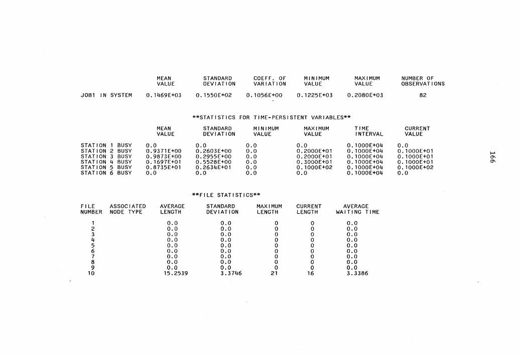
MEAN STANDARD COE FF. OF MINIMUM MAXIMUM NUMBER OF VALUE DEVIATION VARIATION VALUE VALUE OBSERVATIONS
JOB1 IN SYSTEM 0. 1469E+03 O. 1550E+02 0.1056E+OO 0.1225E+03 0.2080[+03 82
**STATISTICS FOR TIME-PERSISTENT VARIABLES**
MEAN STANDARD MINIMUM MAXIMUM TIME CURRENT VALUE DEVIATION VALUE VALUE INTERVAL VALUE
STATION 1 BUSY 0.0 o.o 0.0 0.0 0. 1000E+04 0.0 STATION 2 BUSY 0.9371E+OO 0.2603E+OO 0.0 0.2000E+01 0. 1000E+04 0.1000E+01 1--' STATION 3 BUSY 0.9873E+OO 0.2955E+OO 0.0 0.2000E+01 0.1000E+04 0.1000E+Ol °' STATION 4 BUSY 0.1697E+01 0.5528E+OO o.o 0.3000E+01 0.1000E+04 O. 1000E+01 °' STATION 5 BUSY 0.8735E+01 0.2634E+01 0.0 0. 1000E+02 0.1000E+04 0. 1000E+02 STATION 6 BUSY 0.0 o.o 0.0 0.0 0.1000E+04 0.0
**FILE STATISTICS**
FILE ASSOCIATED AVERAGE STANDARD MAXIMUM CURRENT AVERAGE NUMBER NODE TYPE LENGTH DEVIATION LENGTH LENGTH WA IT .1 NG TI ME
1 0.0 0.0 0 0 0.0 2 0.0 0.0 0 0 0.0 3 0.0 0.0 0 0 0.0 4 0.0 0.0 0 0 0.0 5 o.o 0.0 0 0 0.0 6 0.0 o.o 0 0 0.0 7 0.0 o.o 0 0 0.0 8 0.0 0.0 0 0 o.o 9 o.o 0.0 0 0 0.0
10 15.2539 3.3746 21 16 3.3386
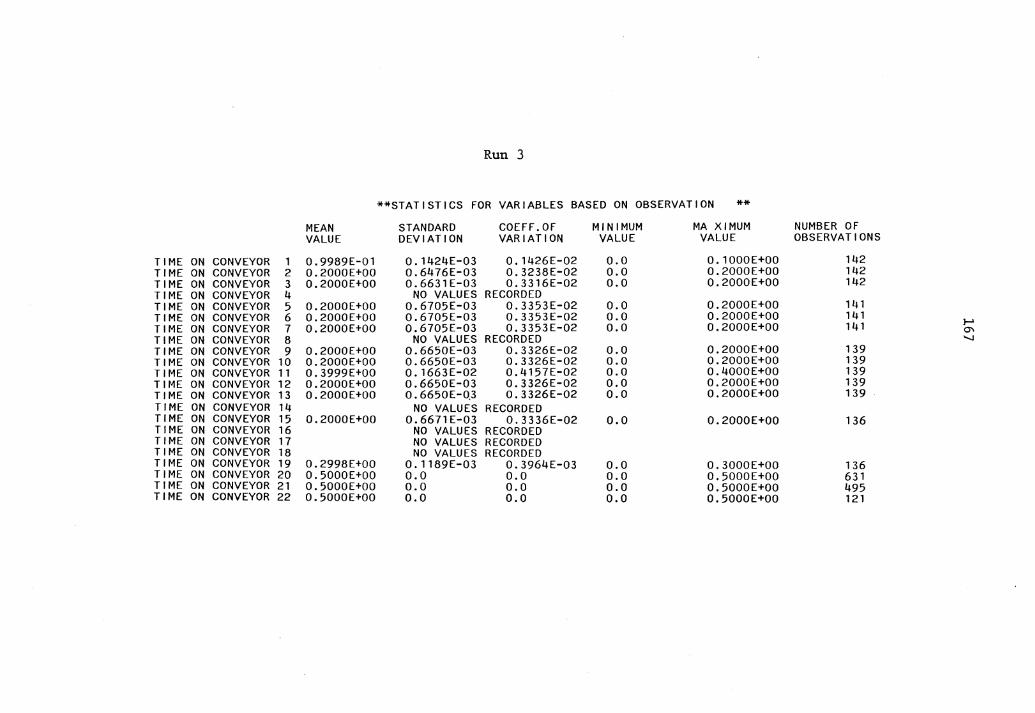
Run 3
**STATISTICS FOR VARIABLES BASED ON OBSERVATION **
MEAN STANDARD COEFF.OF MINIMUM MA XIMUM NUMBER OF VALUE DEVIATION VARIATION VALUE VALUE OBSERVATIONS
TIME ON CONVEYOR 1 0.9989E-01 0. 1424E-03 0.1426E-02 0.0 0.1000E+OO 142 TIME ON CONVEYOR 2 0.2000E+OO 0.6476E-03 0.3238E-02 o.o 0.2000E+OO 142 TIME ON CONVEYOR 3 0.2000E+OO 0.6631E-03 0.3316E-02 0.0 0.2000E+OO 142 TIME ON CONVEYOR 4 NO VALUES RECORDED T ME ON CONVEYOR 5 0.2000E+OO 0.6705E-03 0.3353E-02 0.0 0.2000E+OO 141 T ME ON CONVEYOR 6 0.2000E+OO 0.6705E-03 0.3353E-02 0.0 0.2000E+OO 141 T ME ON CONVEYOR 7 0.2000E+OO 0.6705E-03 0.3353E-02 0.0 0.2000E+OO 141 I-'
O'\ T ME ON CONVEYOR 8 NO VALUES RECORDED "-J
T ME ON CONVEYOR 9 0.2000E+OO 0.6650E-03 0.3326E-02 o.o 0.2000E+OO 139 T ME ON CONVEYOR 10 0.2000E+OO 0.6650E-03 0.3326E-02 0.0 0.2000E+OO 139 T ME ON CONVEYOR 11 0.3999E+OO O. 1663E-02 0.4157E-02 o.o 0.4000E+OO 139 T ME ON CONVEYOR 12 0.2000E+OO 0.6650E-03 0.3326E-02 o.o 0.2000E+OO 139 T ME ON CONVEYOR 13 0.2000E+OO 0. 6650E-0.3 0.3326E-02 0.0 0.2000E+OO 139 T ME ON CONVEYOR 14 NO VALUES RECORDED T ME ON CONVEYOR 15 0.2000E+OO 0.6671E-03 0.3336E-02 0.0 0.2000E+OO 136 T ME ON CONVEYOR 16 NO VALUES RECORDED TIME ON CONVEYOR 17 NO VALUES RECORDED TIME ON CONVEYOR 18 NO VALUES RECORDED TIME ON CONVEYOR 19 0.2998E+OO 0.1189E-03 0.3964E-03 0.0 0.3000E+OO 136 TIME ON CONVEYOR 20 0.5000E+OO o.o 0.0 0.0 0.5000E+OO 631 TIME ON CONVEYOR 21 o.soooE+oo o.o 0.0 o.o 0.5000E+OO 495 TIME ON CONVEYOR 22 0.5000E+OO o.o 0.0 o.o 0.5000E+OO 121
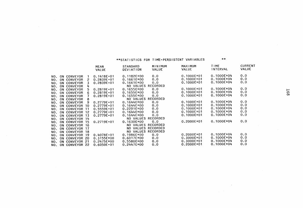
**STATISTICS FOR TIME-PERSISTENT VARIABLES **
MEAN STANDARD MINIMUM MAXIMUM TIME CURRENT VALUE DEVIATION VALUE VALUE INTERVAL VALUE
NO. ON CONVEYOR 1 0. 1418E-Ol 0. 1182E+OO 0.0 O.lOOOE+Ol 0.1000E+04 0.0 NO. ON CONVEYOR 2 0.2839E-Ol 0.1661E+OO 0.0 O.lOOOE+Ol 0.1000E+04 o.o NO. ON CONVEYOR 3 0.2839E-Ol 0.1661E+OO o.o 0. lOOOE+Ol 0.1000E+04 o.o NO. ON CONVEYOR 4 NO VALUES RECORDED NO. ON CONVEYOR 5 0.2819E-Ol O. 1655E+OO 0.0 0. lOOOE+Ol 0.1000E+04 0.0 .J-1 NO. ON CONVEYOR 6 0.2819E-Ol 0.1655E+OO 0.0 O. lOOOE+Ol 0. 1 OOOE+04 o.o Cl'\
NO. ON CONVEYOR 7 0.2819E-Ol 0. 1655E+OO 0.0 O.lOOOE+Ol 0.1000E+04 o.o 00
NO. ON CONVEYOR 8 NO VALUES RECORDED NO. ON CONVEYOR 9 0.2779E-Ol 0.1644E+OO 0.0 0. lOOOE+Ol 0.1000E+04 0.0 NO. ON CONVEYOR 10 0.2779E-Ol 0.1644E+OO 0.0 O. lOOOE+Ol 0. 1000E+04 0.0 NO. ON CONVEYOR 11 0.5559E-Ol 0.2291E+OO 0.0 O.lOOOE+Ol 0.1000E+04 o.o NO. ON CONVEYOR 12 0.2779E-Ol 0.1644E+OO 0.0 O. lOOOE+Ol O.lOOOE+04 0.0 NO. ON CONVEYOR 13 0.2779E-Ol 0.1644E+OO 0.0 O. lOOOE+Ol 0. 1000E+04 0.0 NO. ON CONVEYOR 14 NO VALUES RECORDED NO. ON CONVEYOR 15 0.2719E-Ol 0.1630E+OO 0.0 0.2000E+Ol 0. 1000E+04 o.o NO. ON CONVEYOR 16 NO VALUES RECORDED NO. ON CONVEYOR 17 NO VALUES RECORDED NO. ON CONVEYOR 18 NO VALUES RECORDED NO. ON CONVEYOR 19 0.4078E-Ol 0.1986E+OO 0.0 0.2000E+Ol 0.1000E+04 0.0 NO. ON CONVEYOR 20 0.3155E+OO o.6011E+oo 0.0 0.3000E+Ol 0. 1 OOOE+04 o.o NO. ON CONVEYOR 21 0.2475E+OO 0.5580E+OO 0.0 0.3000E+Ol 0. lOOOE+04 o.o NO. ON CONVEYOR 22 0.6050E-Ol 0.2447E+OO 0.0 0.2000E+Ol 0.1000E+04 0.0
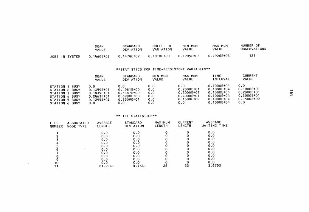
MEAN STANDARD COEFF. OF MINIMUM MAXIMUM NUMBER OF VALUE DEVIATION VARIATION VALUE VALUE OBSERVATIONS
JOB1 IN SYSTEM 0.1460E+03 0.1474E+02 0.1010E+OO 0.1205E+03 0.1926E+03 121
**STATISTICS FOR TIME-PERSISTENT VARIABLES**
MEAN STANDARD MINIMUM MAXIMUM TIME CURRENT VALUE DEVIATION VALUE VALUE INTERVAL VALUE
STATION 1 BUSY 0.0 0.0 0.0 o.o 0.1000E+04 0.0 STATION 2 BUSY 0.1359E+01 0.4981E+OO 0.0 0.2000E+01 0.1000E+04 O. lOOOE+Ol !-' STATION 3 BUSY O. 1439E+01 0.5347E+OO 0.0 0.2000E+01 0.1000E+04 0.2000E+01 CJ' STATION 4 BUSY 0.2463E+01 0.6990E+OO o.o 0.4000E+01 0.1000E+04 0.3000E+01 \0
STATION 5 BUSY 0.1295E+02 0.3909E+01 0.0 0. 1500E+02 0.1000E+04 0. 1500E+02 STATION 6 BUSY o.o o.o 0.0 0.0 O. 1DOOE+04 o.o
**FILE STATISTICS**
FILE ASSOCIATED AVERAGE STANDARD MAXIMUM CURRENT AVERAGE NUMBER NODE TYPE LENGTH DEVIATION LENGTH LENGTH WA I Tl NG Tl ME
1 0.0 0.0 0 0 0.0 2 0.0 0.0 0 0 0.0 3 0.0 0.0 0 0 0.0 4 0.0 0.0 0 0 0.0 5 0.0 0.0 0 0 0.0 6 0.0 0.0 0 0 0.0 7 o.o o.o 0 0 0.0 8 0.0 o.o 0 0 0.0 9 o.o o.o 0 0 0.0
10 o.o 0.0 0 0 0.0 11 21.2247 4.7641 26 22 3.6753
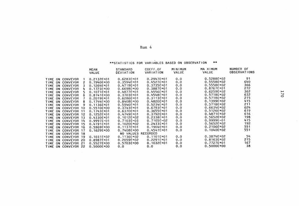
Run 4
**STATISTICS FOR VARIABLES BASED ON OBSERVATION **
MEAN STANDARD COEFF. OF MINIMUM MA XIMUM NUMBER OF VALUE DEVIATION VARIATION VALUE VALUE OBSERVATIONS
T ME ON CONVEYOR 1 0.2132E+01 0.6283E+01 0.2947E+01 0.0 0.5288E+02 91 T ME ON CONVEYOR 2 0.7940E+OO 0.3594E+01 0.4527E+01 0.0 0.5558E+02 640 T ME ON CONVEYOR 3 O. 1264E+01 0.4719E+01 0.3735E+01 0.0 0.5558E+02 366 T ME ON CONVEYOR 4 0. 1723E+OO 0.6698E+OO 0.3887E+01 0.0 0.8767E+01 272 T ME ON CONVEYOR 5 0. 1071 E+Ol 0.4877E+01 0.4556E+01 0.0 0.6259E+02 362 ....... T ME ON CONVEYOR 6 0.8141E+OO 0.3703E+01 0.4548E+01 0.0 0.5718E+02 632 '-l
T ME ON CONVEYOR 7 0.2019E+01 0.6286E+01 0.3113E+01 0.0 0.5718E+02 215 0
T ME ON CONVEYOR 8 0.1744E+OO 0.8408E+OO 0.4820E+01 o.o 0.1399E+02 415 T ME ON CONVEYOR 9 0. 1136E+01 0.5946E+01 0.5234E+01 0.0 0.5718E+02 211 T ME ON CONVEYOR 10 0.5510E+OO 0.3743E+01 0.6793E+01 o.o 0.6634E+02 624 T ME ON CONVEYOR 11 0.1743E+01 0.6370E+01 0.3655E+01 0.0 0.5126E+02 619 T ME ON CONVEYOR 12 0.1252E+01 0.4749E+Q1 0.3792E+01 0.0 0.4871E+02 616 T ME ON CONVEYOR 13 0.4330E+01 0. 1012E+02 0.2338E+01 o.o 0.5652E+02 198 T ME ON CONVEYOR 14 0.9997E-01 0.7103E-03 0.7105E-02 0.0 0.9999E-01 415 T ME ON CONVEYOR 15 0.4191E+01 0.1020E+02 0.2433E+01 0.0 0.5652E+02 192 T ME ON CONVEYOR 16 0.5969E+OO 0.1137E+01 0.1904E+01 o.o 0.2106E+02 551 T ME ON CONVEYOR 17 0. 1629E+OO 0.7408E+OO 0.4547E+01 0.0 0.1040E+02 551 T ME ON CONVEYOR 18 NO VALUES RECORDED TIME ON CONVEYOR 19 0.1031E+02 0. 1136E+02 0.1101E+01 0.0 0.3874E+02 54 TIME ON CONVEYOR 20 0.8987E+01 0.2059E+02 0.2291E+01 0.0 0.8163E+02 215 TIME ON CONVEYOR 21 0.5527E+OO 0.5703E+OO O. 1032E+01 0.0 0.7727E+01 167 TIME ON CONVEYOR 22 0.5000E+OO o.o 0.0 0.0 0.5000E+OO 38
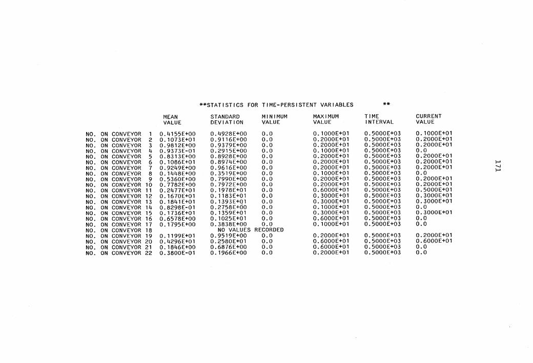
**STATISTICS FOR TIM~-PERSISTENT VARIABLES **
MEAN STANDARD MINIMUM MAXIMUM TIME CURRENT VALUE DEVIATION VALUE VALUE INTERVAL VALUE
NO. ON CONVEYOR 1 0.4155E+OO 0.4928E+OO 0.0 0.1000E+01 0.5000E+03 O. 1000E+01 NO. ON CONVEYOR 2 0.1073E+01 0. 9116E+OO 0.0 0.2000E+01 0.5000E+03 0.2000E+01 NO. ON CONVEYOR 3 0.9812E+OO 0.9379E+OO 0.0 0.2000E+01 0.5000E+03 0.2000E+01 NO. ON CONVEYOR 4 0.9373E-01 0.2915E+OO 0.0 0.1000E+01 0.5000E+03 o.o NO. ON CONVEYOR 5 0.8313E+OO 0.8928E+OO 0.0 0.2000E+01 0.5000E+03 0.2000E+01 NO. ON CONVEYOR 6 0. 1086E+01 0.8974E+OO 0.0 0.2000E+01 0.5000E+03 0.2000E+01 1-' NO. ON CONVEYOR 7 0.9249E+OO 0.9616E+OO 0.0 0.2000E+01 0.5000E+03 0.2000E+01 -...J
NO. ON CONVEYOR 8 0.1448E+OO 0.3519E+OO 0.0 0.1000E+01 0.5000E+03 o.o ........
NO. ON CONVEYOR 9 0.5360E+OO 0.7990E+OO 0.0 0.2000E+01 0.5000E+03 0.2000E+01 NO. ON CONVEYOR 10 0.7782E+OO 0.7972E+OO o.o 0.2000E+01 0.5000E+03 0.2000E+01 NO. ON CONVEYOR 11 0.2477E+01 0. 1978E+01 o.o 0.6000E+01 0.5000E+03 0.5000E+01 NO. ON CONVEYOR 12 0. 1670E+01 0.1183E+01 0.0 0.3000E+01 0.5000E+03 0.3000E+01 NO. ON CONVEYOR 13 0.1841E+01 0.1393E+01 0.0 0.3000E+01 0.5000E+03 0.3000E+01 NO. ON CONVEYOR 14 0.8298E-01 0.2758E+do 0.0 0.1000E+01 0.5000E+03 0.0 NO. ON CONVEYOR 15 0.1736E+01 0.1359E+01 0.0 0.3000E+01 0.5000E+03 0.3000E+01 NO. ON CONVEYOR 16 0.6578E+OO 0.1025E+Ol 0.0 0.6000E+01 0.5000E+03 o.o NO. ON CONVEYOR 17 O. 1795E+OO 0.3838E+OO 0.0 0. 1000E+01 0.5000E+03 o.o NO. ON CONVEYOR 18 NO VALUES RECORDED NO. ON CONVEYOR 19 0.1199E+01 0.9519E+OO 0.0 0.2000E+01 0.5000E+03 0.2000E+01 NO. ON CONVEYOR 20 O. 4296E+01 0.2580E+01 0.0 0.6000E+01 0.5000E+03 0.6000E+01 NO. ON CONVEYOR 21 0.1846E+OO 0.6876E+OO 0.0 0.6000E+01 0.5000E+03 o.o NO. ON CONVEYOR 22 0. 3800E-01 O. 1966E+OO 0.0 0.2000E+01 0.5000E+03 o.o
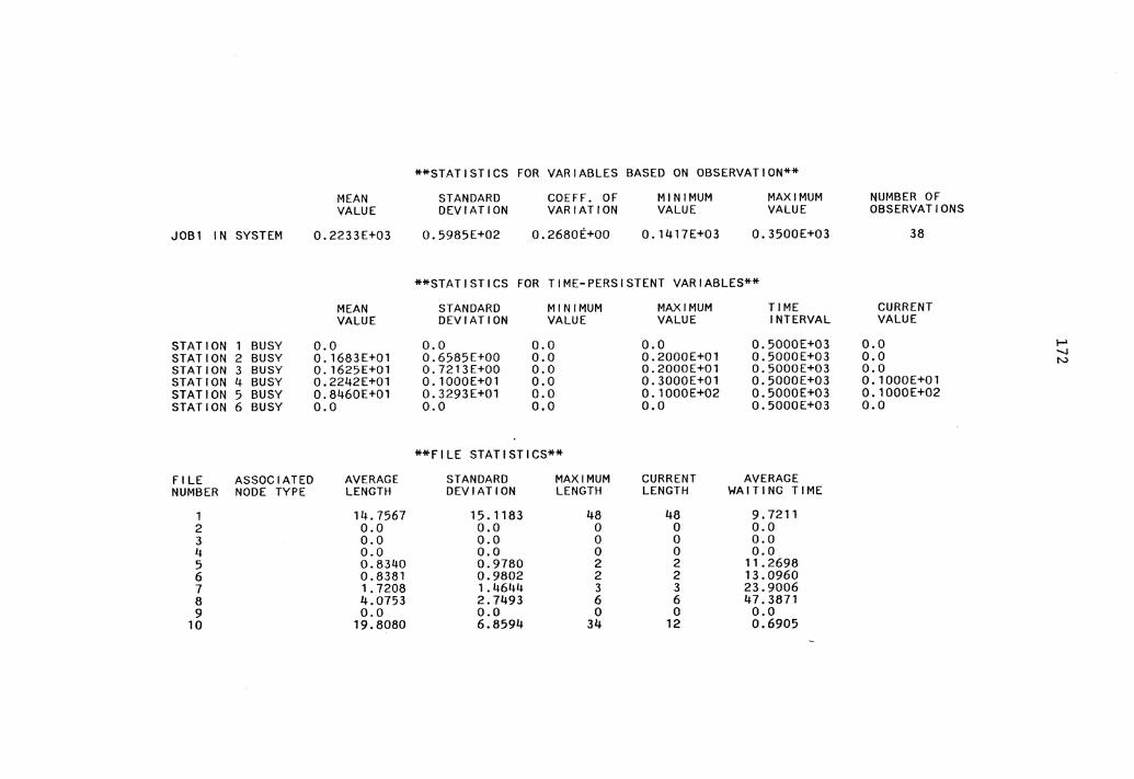
**STATISTICS FOR VARIABLES BASED ON OBSERVATION**
MEAN STANDARD COEFF. OF MINIMUM MAXIMUM NUMBER OF VALUE DEVIATION VARIATION VALUE VALUE OBSERVATIONS
JOBl IN SYSTEM 0.2233E+03 0.5985E+02 0.2680E+OO 0.1417E+03 0.3500E+03 38
**STATISTICS FOR TIME-PERSISTENT VARIABLES**
MEAN STANDARD MINIMUM MAXIMUM TIME CURRENT VALUE DEVIATION VALUE VALUE INTERVAL VALUE
STATION 1 BUSY 0.0 0.0 0.0 0.0 0.5000E+03 0.0 !-"' STATION 2 BUSY 0.1683E+Ol 0.6585E+OO 0.0 0.2000E+Ol 0.5000E+03 0.0 --.!
N STATION 3 BUSY O. 1625E+Ol 0.7213E+OO 0.0 0.2000E+Ol 0.5000E+03 0.0 STATION 4 BUSY 0.2242E+Ol O. lOOOE+Ol 0.0 0.3000E+Ol 0.5000E+03 0. lOOOE+Ol STATION 5 BUSY 0.8460E+Ol 0.3293E+Ol 0.0 0. 1000E+02 0.5000E+03 0. 1000E+02 STATION 6 BUSY 0.0 0.0 0.0 0.0 0.5000E+03 0.0
**FILE STATISTICS**
FILE ASSOCIATED AVERAGE STANDARD MAXIMUM CURRENT AVERAGE NUMBER NODE TYPE LENGTH DEVIATION LENGTH LENGTH WAITING TIME
1 14.7567 15.1183 48 48 9.7211 2 0.0 0.0 0 0 o.o 3 o.o 0.0 0 0 0.0 4 0.0 0.0 0 0 0.0 5 0.8340 0.9780 2 2 11.2698 6 0.8381 0.9802 2 2 13.0960 7 1. 7208 1. 4644 3 3 23.9006 8 4.0753 2.7493 6 6 47.3871 9 0.0 0.0 0 0 0.0
10 19.8080 6.8594 34 12 0.6905
APPENDIX C
USER'S MANUAL
173
174
The design of a material handling system is very criti-
cal if an economic manufacture is desired. Material han-
dling directly affects the production. Perhaps the most
critical step in planning a material handling system is the
evalution of a proposed system design. In evaluating the
performance of conveyor systems, design and operational
problems should be studied together.
This study is conducted to develop a simulation model
in SLAM II to simulate conveyor systems and help the analyst
and designer in evaluation and design of conveyor systems.
The model is capable of simulating different conveyor sys-
tems regardless of what kind of conveyor is being used.
This manual, in conjunction with the report, is to
describe the model (program) and help user understand the
flow of model and relationship among subroutines used. Even
though the program is documented, a brief description of
what each subroutine does is also presented.
Model uses a number of attributes, and files. Descrip-
tion of events and variables is also presented.
Attributes: Attributes play an important role in storing
informatin about a part. There are a number of attributes
associated with each entity. These attributes identify the
part, part route, part path; etc. A description of the
attributes is as follows:
Attribute 1 -Arrival time to the system
Attribute 2
Attribute 3
Attribute 4
Attribute 5
Attribute 6
Attribute 7
Attribute 8
Attribute 9
Attribute 10
Attribute 11
Attribute 12
Attribute 13
Attribute 14
175
-Last station visited (Station I.D.)
-Next station to be visted (Station
I .D.)
-Part type
-Number of nodes visited on the current
path
-Number of stations visited in the sys-
tem
-Total number of nodes on the current
path
-Arrival time on a conveyor section
-Last arc visted (Arc I.D.)
-Next arc to be visited (Arc I.D.)
-Last node visited on the current path
(first node)
-Next node to be visited on the current
path (second node)
-Third node on the path (if any)
-Fourth node on the path (if any) and so
on.
Attributes 11 and onwards are used to store the current
path of a part. For example: if the path between station 2
and 5 is 2, 6, 8, and 15, then
Attribute (11) = 2
Attribute (12) = 6
Attribute (13) = 8
176
Attribute (14) = 15.
After each node is visited attributes 11 and 12 are
assigned to their new values. Thus after the first node, the
values will be
Attribute (11) = 6
Attribute (12) = 8
Attribute (13) = 8
Attribute (14) = 15.
The maximum number of attributes associated with a part
Ii I iS
10 + max (NODPTH). 1
Where (NODPTH). is the number of nodes on a path bet-1
ween two stations for part type i. There is a limit of 100
on the total number of attributes.
Files:
Files are used in storing entities rather than informa-
tion about entities. When an entity cannot advance in the
system, it is placed in a file. A number of files are used
in the model which are used under different conditions and
at different places in the system. Each service areas has a
file to store entities whily they are waiting for service.
When a part is at a node and cannot move in the system it is
placed in file 1 or 3 depending on the class of conveyor.
Examples will help understand the use of files. At the pre-
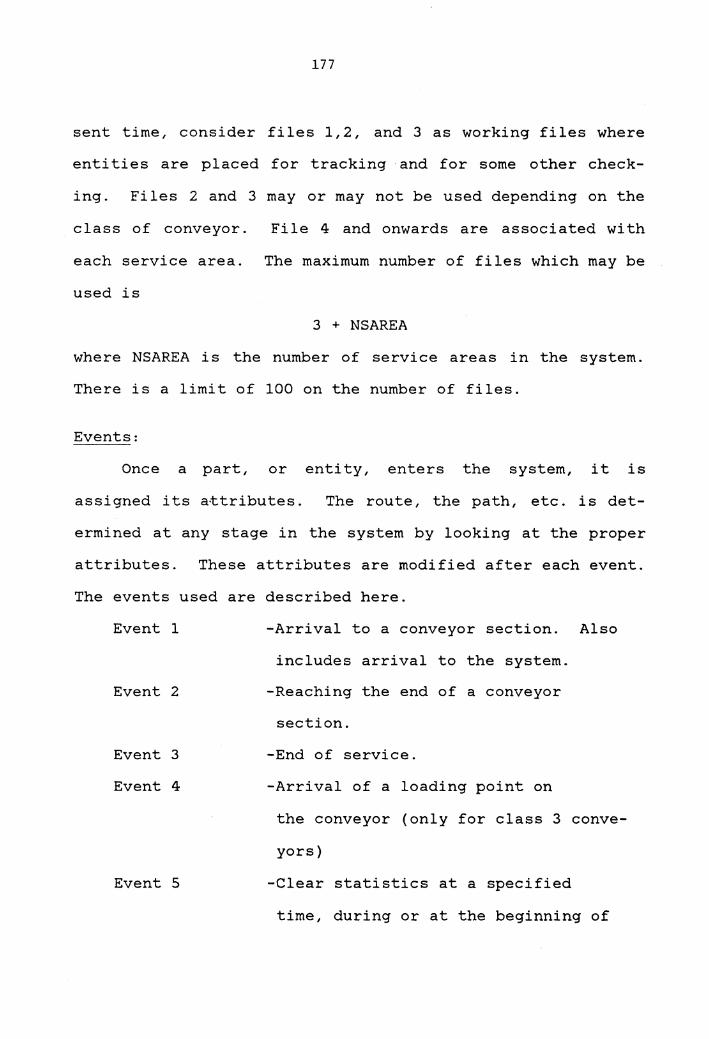
177
sent time, consider files 1,2, and 3 as working files where
entities are placed for tracking and for some other check-
ing. Files 2 and 3 may or may not be used depending on the
class of conveyor. File 4 and onwards are associated with
each service area. The maximum number of files which may be
used is
3 + NSAREA
where NSAREA is the number of service areas in the system.
There is a limit of 100 on the number of files.
Events:
Once a part, or entity, enters the system, it is
assigned its attributes. The route, the path, etc. is det-
ermined at any stage in the system by looking at the proper
attributes. These attributes are modified after each event.
The events used are described here.
Event 1
Event 2
Event 3
Event 4
Event 5
-Arrival to a conveyor section. Also
includes arrival to the system.
-Reaching the end of a conveyor
section.
-End of service.
-Arrival of a loading point on
the conveyor (only for class 3 conve-
yors)
-Clear statistics at a specified
time, during or at the beginning of
178
a simulation period.
Event 6 -End of simulation period.
Global variables, XX(.), are used to define the status
of a service area. For example, if XX(2) has a value 5,
then there are five servers busy at station 2 at that time.
If an XX(.) variable has a value of zero, it means none of
the servers are busy at a specific station at that time.
The variables used in the model are consistent in nota-
tion throughout the model.
Table 7.
These variables are defined in
Detail on what each subroutine does and the linkages
among subroutines is presented in Appendix C. A program
listing is included in Appendix A.
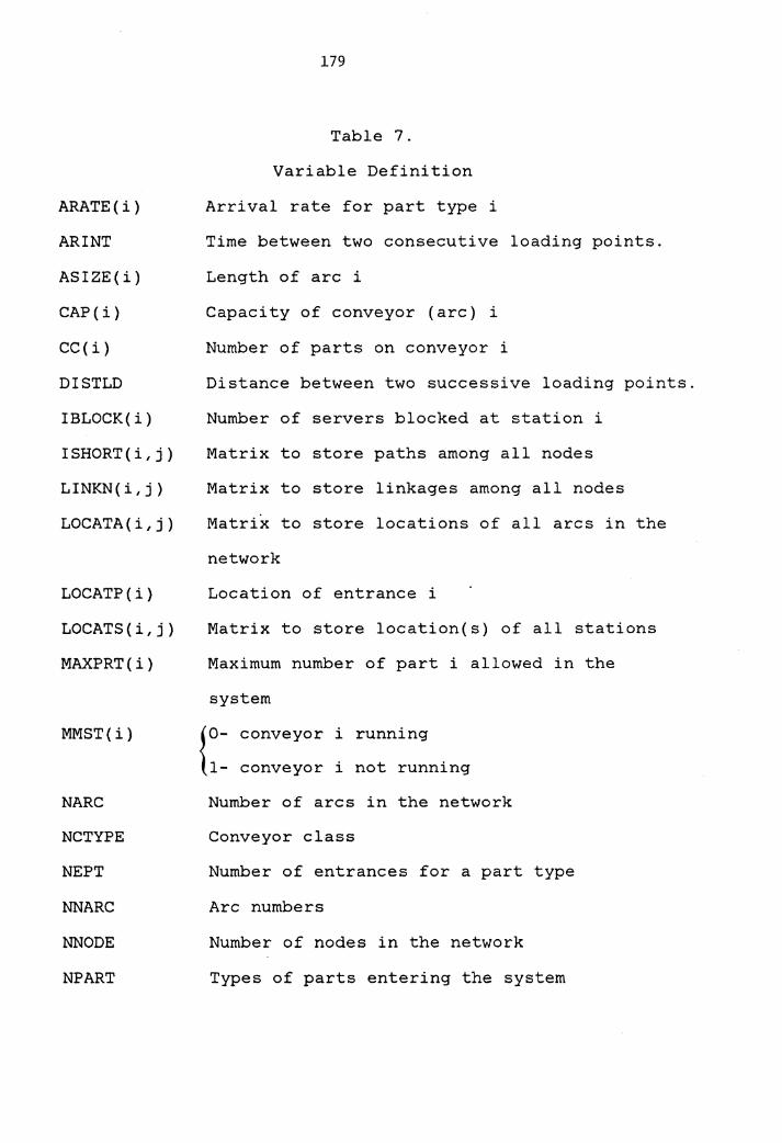
ARATE(i)
ARI NT
ASIZE(i)
CAP(i)
CC(i)
DISTLD
IBLOCK(i)
ISHORT(i,j)
LINKN(i,j)
LOCATA(i,j)
LOCATP(i)
LOCATS(i,j)
MAXPRT(i)
MMST(i)
NARC
NC TYPE
NEPT
NNARC
NNODE
NP ART
179
Table 7.
Variable Definition
Arrival rate for part type i
Time between two consecutive loading points.
Length of arc i
Capacity of conveyor (arc) i
Number of parts on conveyor i
Distance between two successive loading points.
Number of servers blocked at station i
Matrix to store paths among all nodes
Matrix to store linkages among all nodes
Matrix to store locations of all arcs in the
network
Location of entrance i
Matrix to store location(s) of all stations
Maximum number of part i allowed in the
system
{0- conveyor i running
1- conveyor i not running
Number of arcs in the network
Conveyor class
Number of entrances for a part type
Arc numbers
Number of nodes in the network
Types of parts entering the system
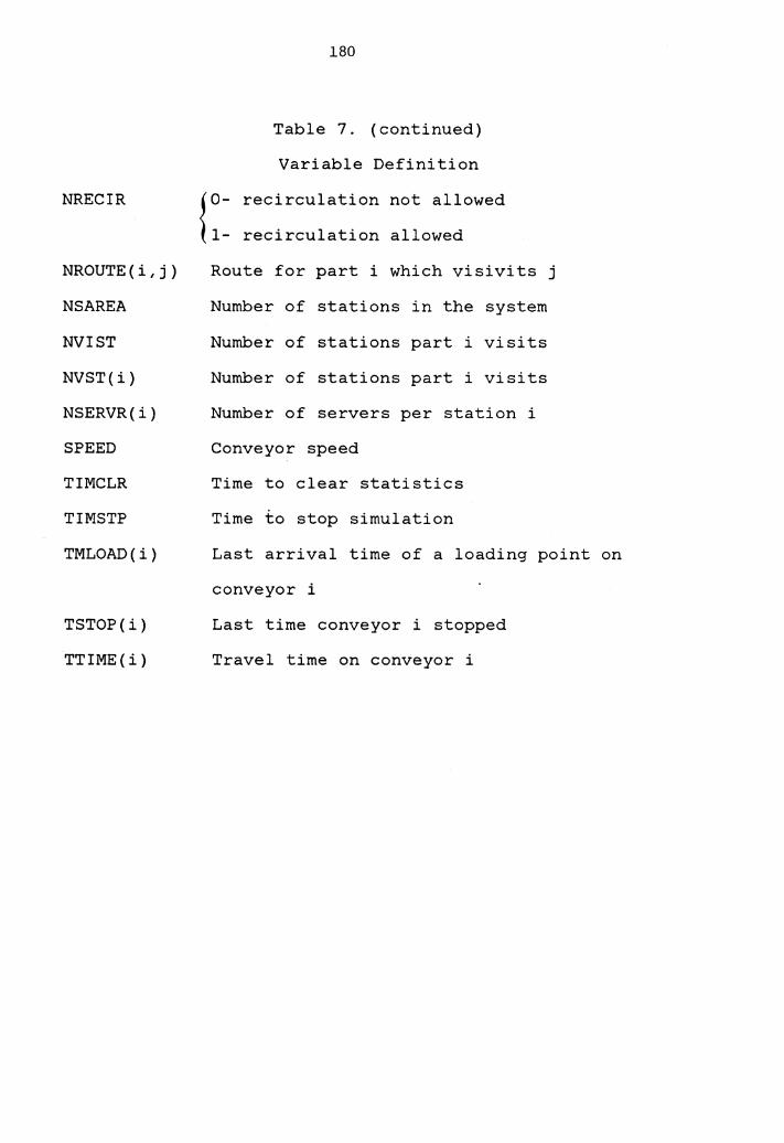
NRECIR
NROUTE(i,j)
NS AREA
NVIST
NVST(i)
NSERVR(i)
SPEED
TIMCLR
TIMSTP
TMLOAD(i)
TSTOP(i)
TTIME(i)
180
Table 7. (continued)
Variable Definition
{0- recirculation not allowed
1- recirculation allowed
Route for part i which visivits j
Number of stations in the system
Number of stations part i visits
Number of stations part i visits
Number of servers per station i
Conveyor speed
Time to clear statistics
Time to stop simulation
Last arrival time of a loading point on
conveyor i
Last time conveyor i stopped
Travel time on conveyor i
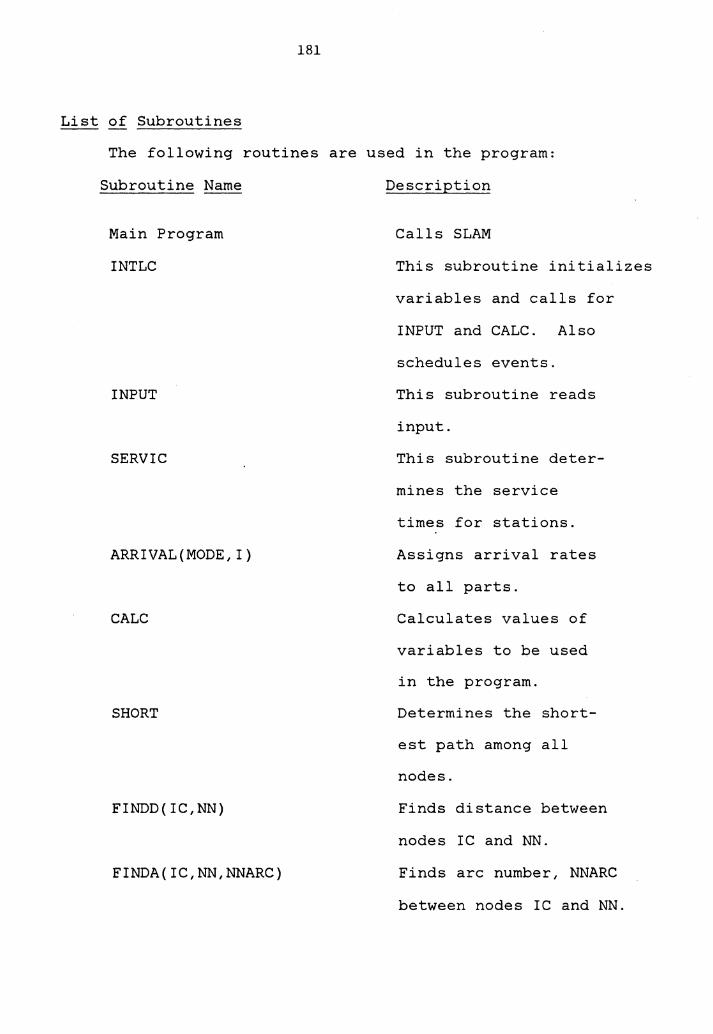
181
List of Subroutines
The following routines are used in the program:
Subroutine Name
Main Program
INTLC
INPUT
SERVIC
ARRIVAL(MODE,I)
CALC
SHORT
FINDD(IC,NN)
FINDA(IC,NN,NNARC)
Description
Calls SLAM
This subroutine initializes
variables and calls for
INPUT and CALC. Also
schedules events.
This subroutine reads
input.
This subroutine deter-
mines the service
times for stations.
Assigns arrival rates
to all parts.
Calculates values of
variables to be used
in the program.
Determines the short-
est path among all
nodes.
Finds distance between
nodes IC and NN.
Finds arc number, NNARC
between nodes IC and NN.
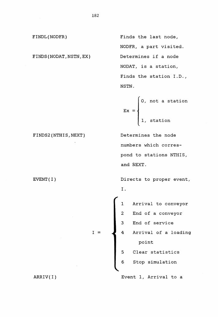
182
FINDL(NODFR)
FINDS(NODAT,NSTN,EX)
FINDS2(NTHIS,NEXT)
EVENT( I)
I =
ARRIV(I)
Finds the last node,
NODFR, a part visited.
Determines if a node
NODAT, is a station,
Finds the station I.D.,
NSTN.
0, not a station
Ex = 1, station
Determines the node
numbers which corres-
pond to stations NTHIS,
and NEXT.
Directs to proper event,
I.
1 Arrival to conveyor
2 End of a conveyor
3 End of service
4 Arrival of a loading
point
5 Clear statistics
6 Stop simulation
Event 1, Arrival to a
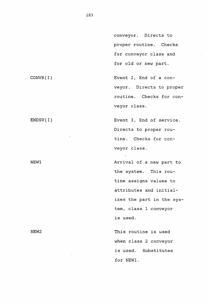
183
CONVR(I)
ENDSV(I)
NEWl
NEW2
conveyor. Directs to
proper routine. Checks
for conveyor class and
for old or new part.
Event 2, End of a con-
veyor. Directs to proper
routine. Checks for con-
veyor class.
Event 3, End of service.
Directs to proper rou-
tine. Checks for con-
veyor class.
Arrival of a new part to
the system. This rou-
tine assigns values to
attributes and initial-
izes the part in the sys-
tem, class 1 conveyor
is used.
This routine is used
when class 2 conveyor
is used. Substitutes
for NEWl.
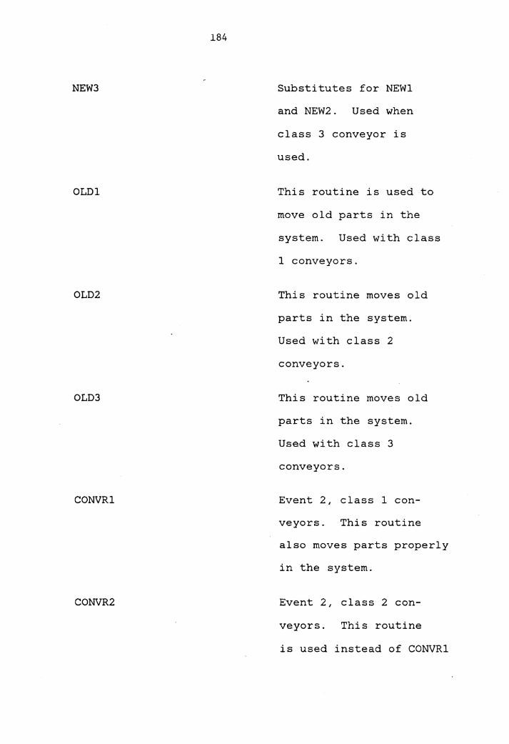
184
NEW3
OLDl
OLD2
OLD3
CONVRl
CONVR2
Substitutes for NEWl
and NEW2. Used when
class 3 conveyor is
used.
This routine is used to
move old parts in the
system. Used with class
1 conveyors.
This routine moves old
parts in the system.
Used with class 2
conveyors.
This routine moves old
parts in the system.
Used with class 3
conveyors.
Event 2, class 1 con-
veyors. This routine
also moves parts properly
in the system.
Event 2, class 2 con-
veyors. This routine
is used instead of CONVRl
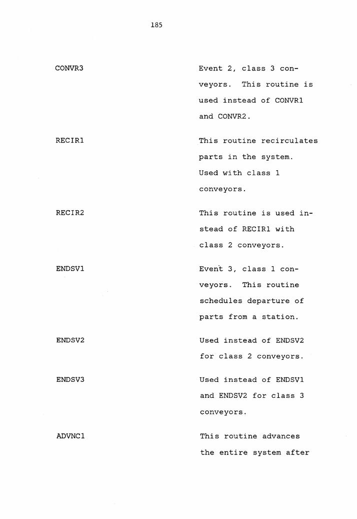
185
CONVR3
RECIRl
RECIR2
ENDSVl
ENDSV2
ENDSV3
ADVNCl
Event 2, class 3 con-
veyors. This routine is
used instead of CONVRl
and CONVR2.
This routine recirculates
parts in the system.
Used with class 1
conveyors.
This routine is used in-
stead of RECIRl with
class 2 conveyors.
Event 3, class 1 con-
veyors. This routine
schedules departure of
parts from a station.
Used instead of ENDSV2
for class 2 conveyors.
Used instead of ENDSVl
and ENDSV2 for class 3
conveyors.
This routine advances
the entire system after
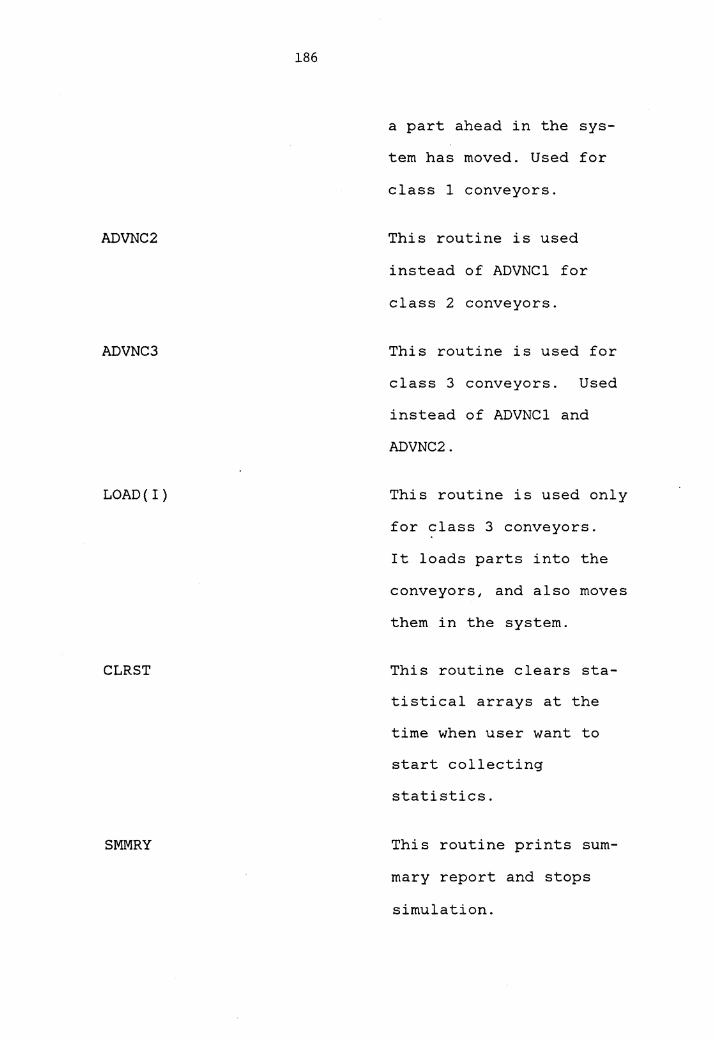
186
ADVNC2
ADVNC3
LOAD( I)
CLRST
SMMRY
a part ahead in the sys-
tem has moved. Used for
class 1 conveyors.
This routine is used
instead of ADVNCl for
class 2 conveyors.
This routine is used for
class 3 conveyors. Used
instead of ADVNCl and
ADVNC2.
This routine is used only
for class 3 conveyors.
It loads parts into the
conveyors, and also moves
them in the system.
This routine clears sta-
tistical arrays at the
time when user want to
start collecting
statistics.
This routine prints sum-
mary report and stops
simulation.
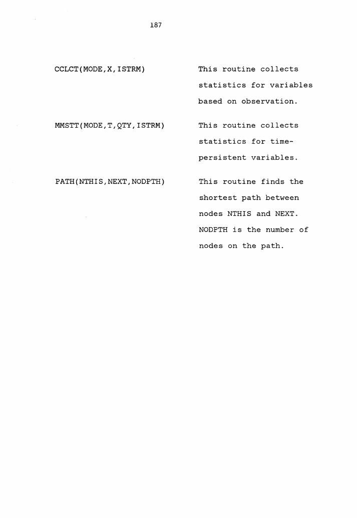
187
CCLCT(MODE,X,ISTRM)
MMSTT(MODE,T,QTY,ISTRM)
PATH(NTHIS,NEXT,NODPTH)
This routine collects
statistics for variables
based on observation.
This routine collects
statistics for time-
persistent variables.
This routine finds the
shortest path between
nodes NTHIS and NEXT.
NODPTH is the number of
nodes on the path.
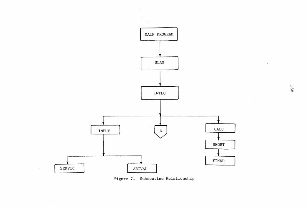
MAIN PROGRAM
SLAM
INTLC
INPUT
SERVIC ARIVAL
Figure 7. Subroutine Relationship
CALC
SHORT
FINDD
I-' co co
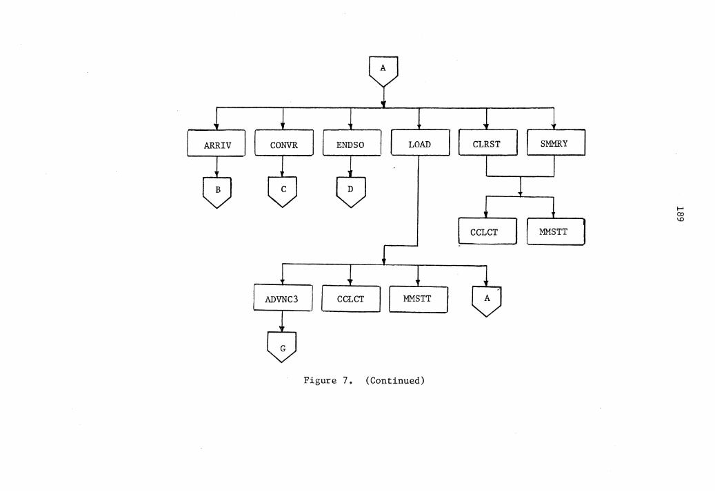
ARR IV CONVR END SO LOAD
ADVNC3 CCL CT MMSTT
Figure 7. (Continued)
CLRST
CCL CT MMSTT
t-' o:i
"°
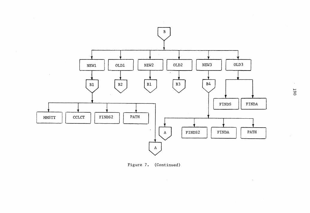
OLDl OLD2
MMSTT CCL CT FINDS2 PATH
Figure 7. (Continued)
NEW3
FINDS
FINDS2 FIND A
FINDA
PATH
..... '° 0
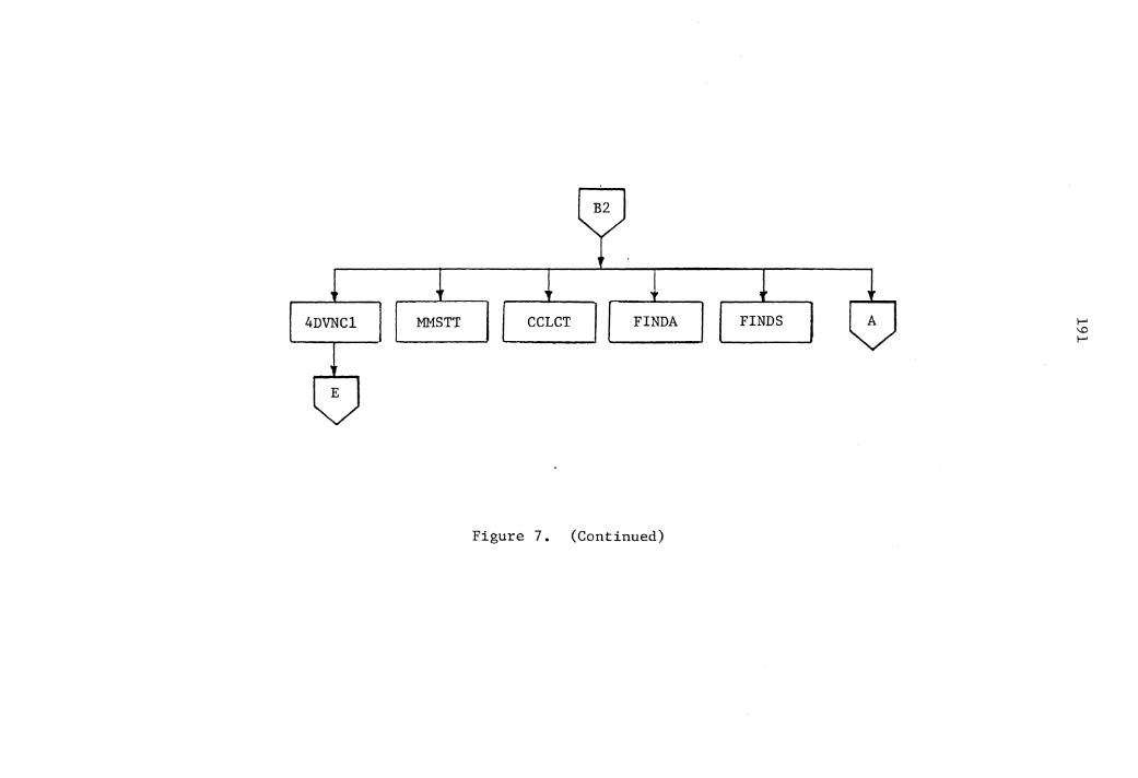
MMSTT CCLCT FINDA
Figure 7. (Continued)
FINDS I-' '° I-'
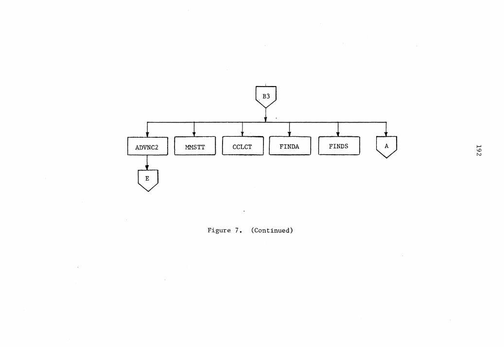
MMSTT CCL CT FINDA
Figure 7. (Continued)
FINDS I-' \.0 N
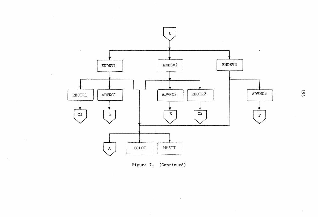
ENDSVl ENDSV2
RECIRl ADVNCl ADVNC2
MMSTT
Figure 7. (Continued)
ENDSV3
RECIR2 ADVNC3 I-'
'° w
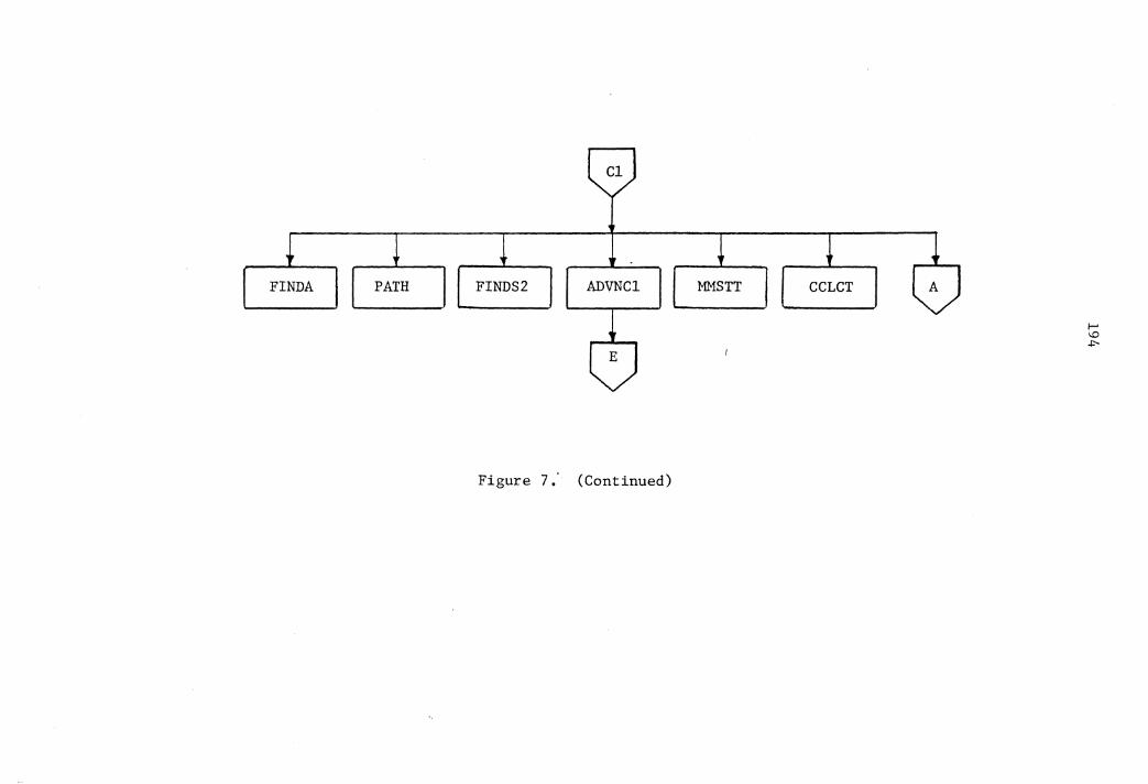
'"rj
'"rj
f-'·
H
(JQ
z i::
t:!
ti
(/)
(!)
N
._....
,......_
(")
E; 0 ::l
rt
~
f-'·
::l
(")
i:: 1--
1 (!)
0.
. '-
'
~ en
t-3
t-3
~61
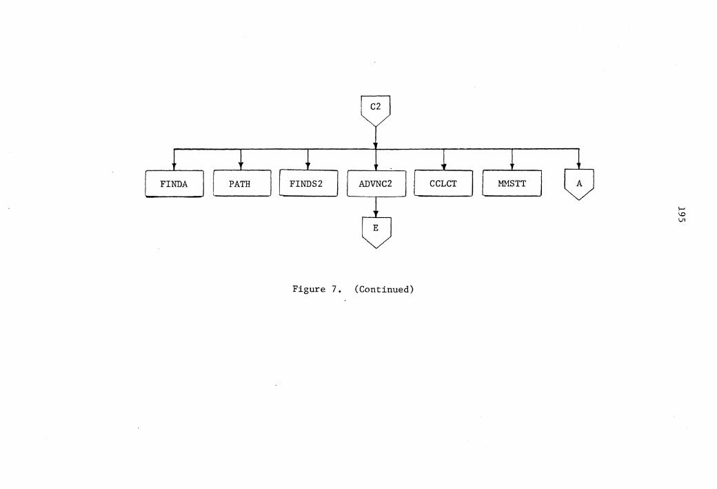
>zj
>zj
I-'·
H
OQ
z
i:: t::I
rt
r:n
ro
N
-...J ,.....
(")
~ 0 ::l
rt
;;§
(")
N
I-'·
(")
::l
N
i:: ro 0..
"-/
(")
(") t""'
(") t-3
~6T
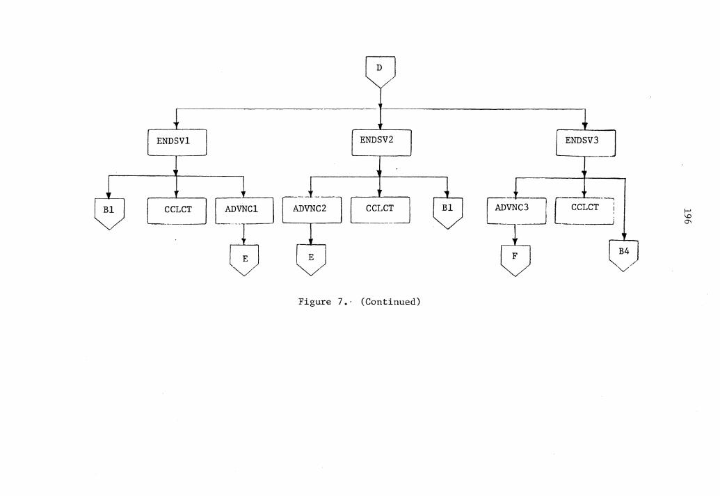
D
ENDSVl ENDSV2
~~ v
ADVNC2
Figure 7.· (Continued)
ENDSV3
[AD~~J [-~CT·--;
~ -- ,.... v ""-v/
I-' \.0 O"\
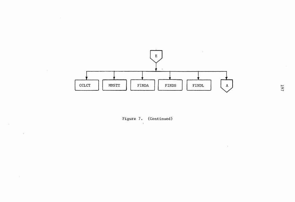
L61
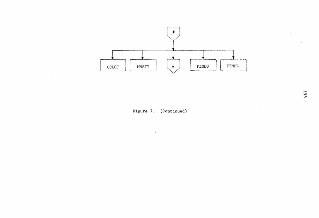
861
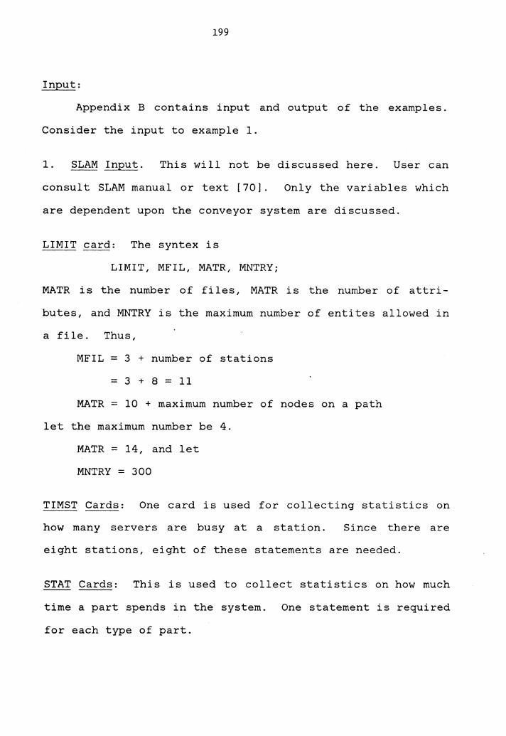
199
Input:
Appendix B contains input and output of the examples.
Consider the input to example 1.
1. SLAM Input. This will not be discussed here. User can
consult SLAM manual or text [70]. Only the variables which
are dependent upon the conveyor system are discussed.
LIMIT card: The syntex is
LIMIT, MFIL, MATR, MNTRY;
MATR is the number of files, MATR is the number of attri-
butes, and MNTRY is the maximum number of entites allowed in
a file. Thus,
MFIL = 3 + number of stations
= 3 + 8 = 11
MATR = 10 + maximum number of nodes on a path
let the maximum number be 4.
MATR = 14, and let
MNTRY = 300
TIMST Cards: One card is used for collecting statistics on
how many servers are busy at a station. Since there are
eight stations, eight of these statements are needed.
STAT Cards: This is used to collect statistics on how much
time a part spends in the system. One statement is required
for each type of part.
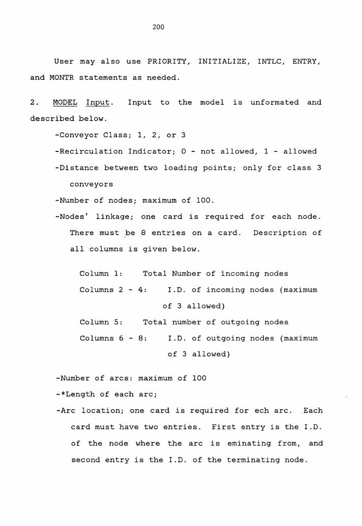
200
User may also use PRIORITY, INITIALIZE, INTLC, ENTRY,
and MONTR statements as needed.
2. MODEL Input. Input to the model is unformated and
described below.
-Conveyor Class; l, 2, or 3
-Recirculation Indicator; 0 - not allowed, 1 - allowed
-Distance between two loading points; only for class 3
conveyors
-Number of nodes; maximum of 100.
-Nodes' linkage; one card is required for each node.
There must be 8 entries on a card. Description of
all columns is given below.
Column 1: Total Number of incoming nodes
Columns 2 4: I.D. of incoming nodes (maximum
of 3 allowed)
Column 5: Total number of outgoing nodes
Columns 6 - 8: I.D. of outgoing nodes (maximum
of 3 allowed)
-Number of arcs: maximum of 100
-*Length of each arc;
-Arc location; one card is required for ech arc. Each
card must have two entries. First entry is the I.D.
of the node where the arc is eminating from, and
second entry is the I.D. of the terminating node.
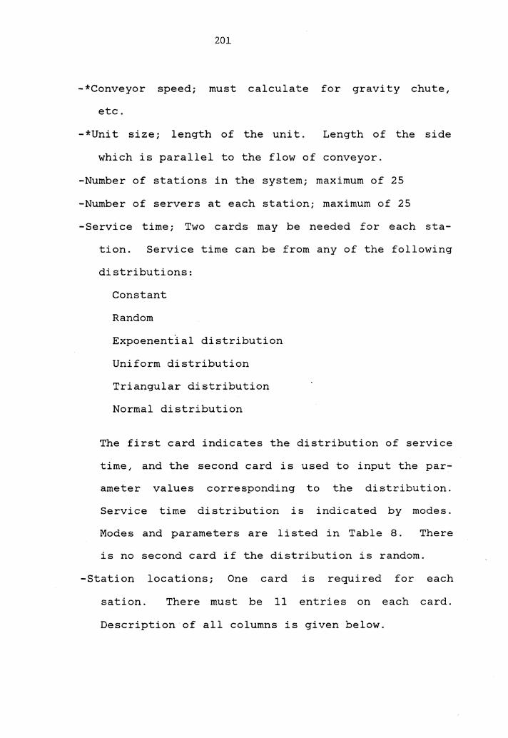
201
-*Conveyor speed; must calculate for gravity chute,
etc.
-*Unit size; length of the unit. Length of the side
which is parallel to the flow of conveyor.
-Number of stations in the system; maximum of 25
-Number of servers at each station; maximum of 25
-Service time; Two cards may be needed for each sta-
tion. Service time can be from any of the following
distributions:
Constant
Random
Expoenential distribution
Uniform distribution
Triangular distribution
Normal distribution
The first card indicates the distribution of service
time, and the second card is used to input the par-
ameter values corresponding to the distribution.
Service time distribution is indicated by modes.
Modes and parameters are listed in Table 8. There
is no second card if the distribution is random.
-Station locations; One card is required for each
sation. There must be 11 entries on each card.
Description of all columns is given below.
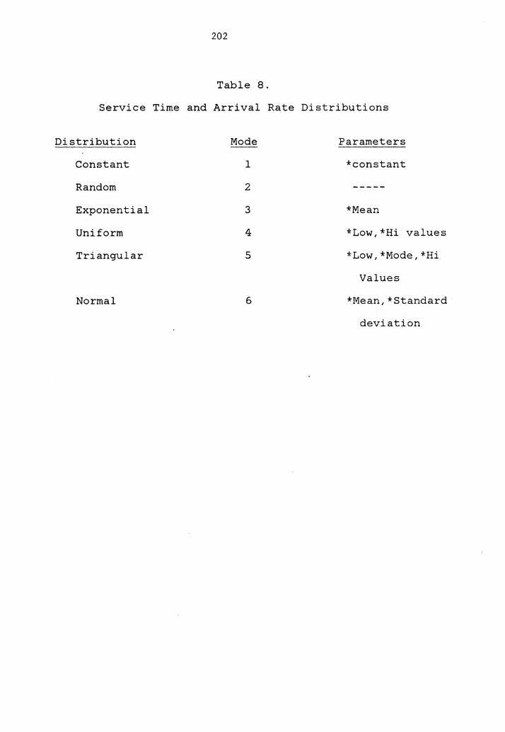
202
Table 8.
Service Time and Arrival Rate Distributions
Distribution
Constant
Random
Exponential
Uniform
Triangular
Normal
Mode
1
2
3
4
5
6
Parameters
*constant
*Mean
*Low,*Hi values
*Low, *Mode, *Hi
Values
*Mean,*Standard
deviation
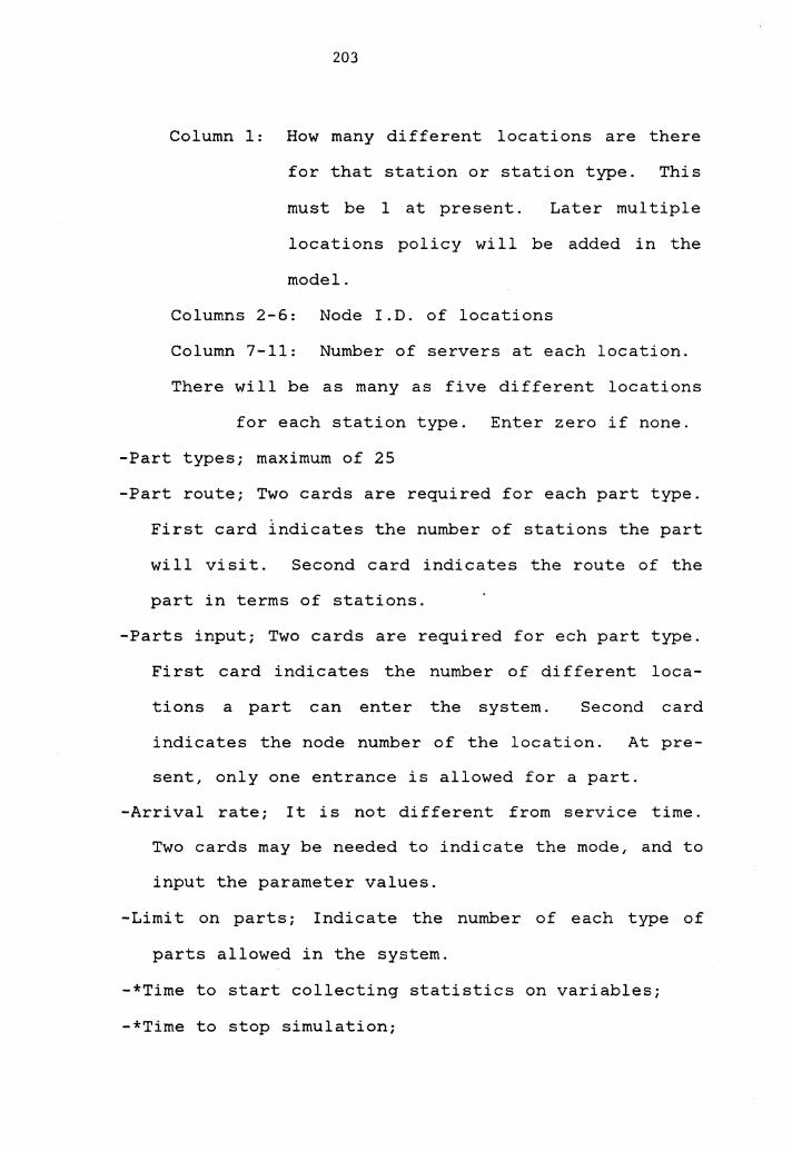
203
Column 1: How many different locations are there
for that station or station type. This
must be 1 at present. Later multiple
locations policy will be added in the
model.
Columns 2-6: Node I.D. of locations
Column 7-11: Number of servers at each location.
There will be as many as five different locations
for each station type. Enter zero if none.
-Part types; maximum of 25
-Part route; Two cards are required for each part type.
First card indicates the number of stations the part
will visit. Second card indicates the route of the
part in terms of stations.
-Parts input; Two cards are required for ech part type.
First card indicates the number of different loca-
tions a part can enter the system. Second card
indicates the node number of the location. At pre-
sent, only one entrance is allowed for a part.
-Arrival rate; It is not different from service time.
Two cards may be needed to indicate the mode, and to
input the parameter values.
-Limit on parts; Indicate the number of each type of
parts allowed in the system.
-*Time to start collecting statistics on variables;
-*Time to stop simulation;
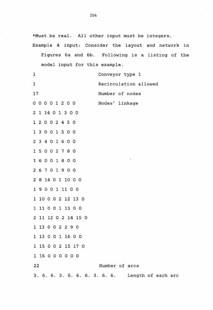
204
*Must be real. All other input must be integers.
Example 4 input: Consider the layout and network in
Figures 6a and 6b. Following is a listing of the
model input for this example.
1 Conveyor type 1
1 Recirculation allowed
17 Number of nodes
0 0 0 0 1 2 0 0
2 1 14 0 1 3 0 0
12002450
1 3 0 0 1 5 0 0
2 3 4 0 1 6 0 b
1 5 0 0 2 7 8 0
1 6 0 0 1 8 0 0
2 6 7 0 1 9 0 0
2 8 14 0 1 10 0 0
1 9 0 0 1 11 0 0
1 10 0 0 2 12 13 0
1 11 0 0 1 13 0 0
2 11 12 0 2 14 15 0
1 13 0 0 2 2 9 0
1 13 0 0 1 16 0 0
1 15 0 0 2 15 17 0
1 16 0 0 0 0 0 0
22
Nodes' linkage
Number of arcs
3. 6. 6. 3. 6. 6. 6. 3. 6. 6. Length of each arc
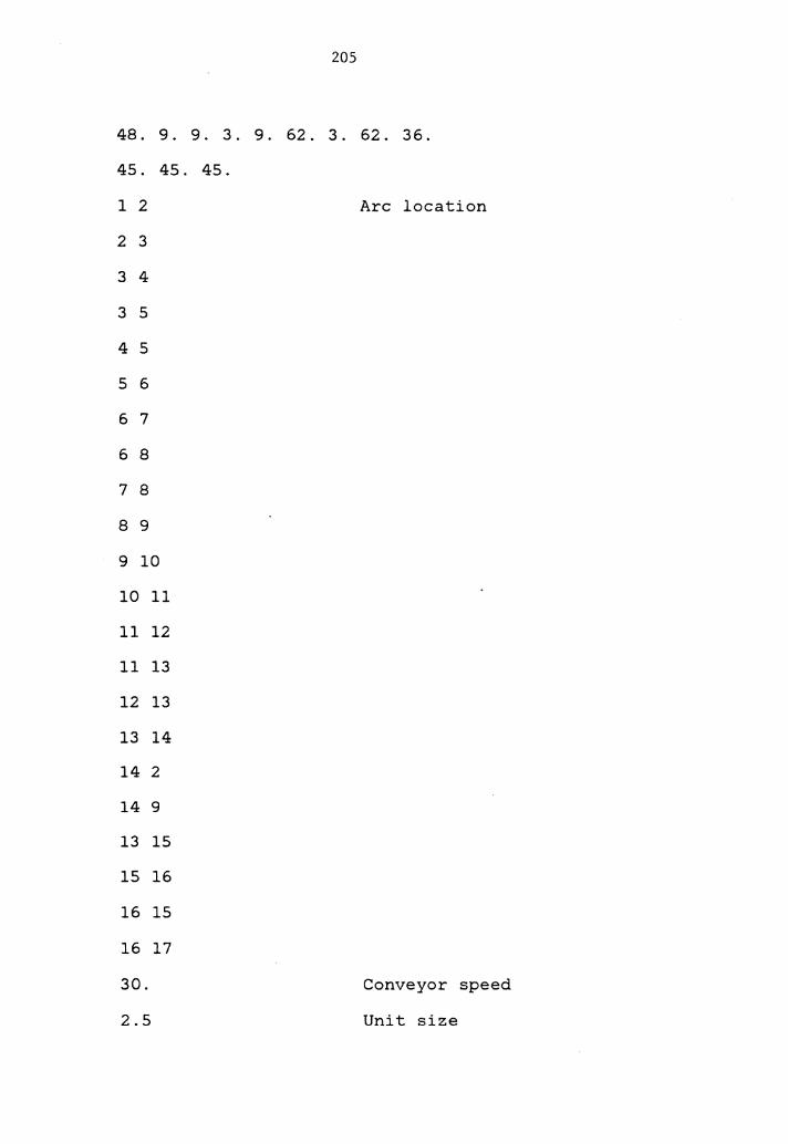
205
48. 9. 9. 3. 9. 62. 3. 62. 36.
45. 45. 45.
1 2
2 3
3 4
3 5
4 5
5 6
6 7
6 8
7 8
8 9
9 10
10 11
11 12
11 13
12 13
13 14
14 2
14 9
13 15
15 16
16 15
16 17
30.
2.5
Arc location
Conveyor speed
Unit size
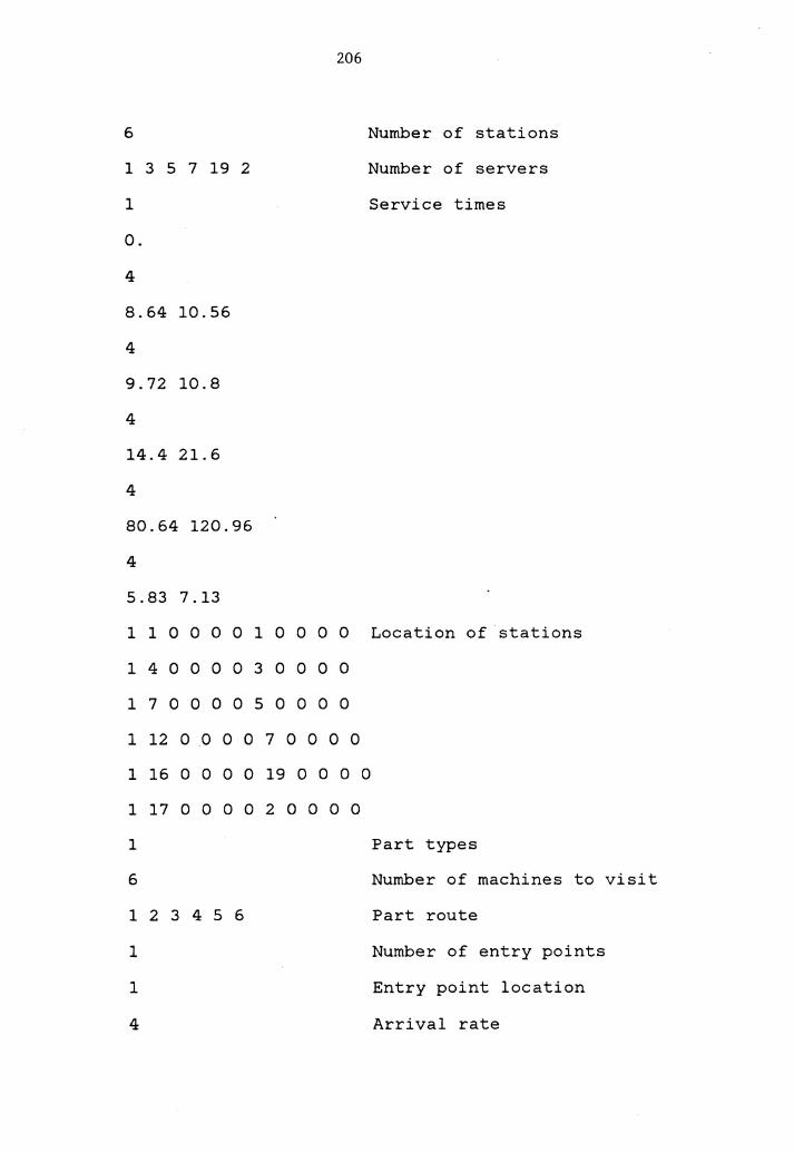
6
1 3 5 7 19 2
1
0.
4
8.64 10.56
4
9.72 10.8
4
14.4 21. 6
4
80.64 120.96
4
5.83 7.13
1 1 0 0 0 0
1 4 0 0 0 0
1 7 0 0 0 0
1 12 0 0 0
1 16 0 0 0
1 17 0 0 0
1
6
123456
1
1
4
0
0
0
1
3
5
206
0 0 0 0
0 0 0 0
0 0 0 0
7 0 0 0 0
Number of stations
Number of servers
Service times
Location of stations
19 0 0 0 0
2 0 0 0 0
Part types
Number of machines to visit
Part route
Number of entry points
Entry point location
Arrival rate
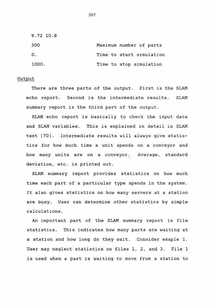
9.72 10.8
300
0.
1000.
Output
207
Maximum number of parts
Time to start simulation
Time to stop simulation
There are three parts of the output. First is the SLAM
echo report. Second is the intermediate results.
summary report is the third part of the output.
SLAM
SLAM echo report is basically to check the input data
and SLAM variables. This is explained in detail in SLAM
text [70]. Inte~mediate results will always give statis-
tics for how much time a unit spends on a conveyor and
how many uni ts are on a conveyor. Average, standard
deviation, etc. is printed out.
SLAM summary report provides statistics on how much
time each part of a particular type spends in the system.
It also gives statistics on how many servers at a station
are busy. User can determine other statistics by simple
calculations.
An important part of the SLAM summary report is file
statistics. This indicates how many parts are waiting at
a station and how long do they wait. Consider exaple 1.
User may neglect statistics on files 1, 2, and 3. File 1
is used when a part is waiting to move from a station to
208
a conveyor, or from another conveyor if the node between
the two conveyors is not a station. Files 2 and 3 are
not used for class 1 conveyors. File 4 through the maxi-
mum number of user defined files are used when a part is
waiting for service at a station or while waiting to go
to another conveyor which is not available. Last file,
file 12, is of no interest to the user.
All this information can be helpful in making design
decisions and evaluting alternatives. This is discussed
in Chapter 5.

The vita has been removed from the scanned document
A GENERALIZED SIMULATION MODEL FOR THE
DESIGN OF A CONVEYOR SYSTEM
by
Asif Manzoor Shaikh
(ABSTRACT)
A simulation model is developed in SLAM II to study and
analyze conveyor systems.. The adequacy of the model is
tested by applying it to a conveyor layout as well as some
variant designs. 1he problem of modeling large systems is
reduced by decomposing the system into smaller segments
(subsystems). Different types of conveyors are considered.
Programming modules are prepared for feasible conveyor types
and segments. These simulation modules are integrated into
a system.