Embed Size (px)
Citation preview

A Generic Theory of the Integer
Quantum Hall Effect
Yu Shen
A Dissertation
Presented to the Faculty
of Princeton University
in Candidacy for the Degree
of Doctor of Philosophy
Recommended for Acceptance
by the Department of
Physics
Adviser: Professor F. D. M. Haldane
September 2017

c© Copyright by Yu Shen, 2017.
All rights reserved.
Abstract
The integer quantum Hall effect (IQHE) is usually modeled by a Galilean or rotation-
ally invariant Hamiltonian. These are not generic symmetries for electrons moving
in a crystal background and can potentially confuse non-topological quantities with
topological ones and identify otherwise distinct geometrical properties. In this thesis
we present a generic theory for the IQHE. First we show that a generic guiding-center
coherent state, defined by a natural metric in each Landau level, has the form of an
antiholomorphic function times an exponential factor. Then by numerically solving
the eigen problem for a quartic Hamiltonian and finding the roots of the antiholomor-
phic part we are able to define a topological spin sn = n + 12
where n is the number
of central roots that are enclosed by the semiclassical orbit. We derive a generic
formula for the Hall viscosity in the absence of rotational symmetry and show that
the previous interpretation of the scalar Hall viscosity as the “intrinsic orbital angu-
lar momentum” breaks down since the concept of angular momentum requires the
presence of rotational symmetry. We also calculate generic electromagnetic responses
and differentiate between universal terms that are diagonal with respect to Landau
level index and non-universal terms that depend on inter-Landau-level mixing. We
conclude that the generic theory offers a fundamental definition for the topological
spin and reveals finer structure in the geometrical properties of the IQHE.
iii

Acknowledgements
The past five years have been one of the most unforgettable chapters in my life. I
feel so lucky and honored to be able to work with Prof. F. D. M. Haldane, one
of the greatest physicists in the world, who has taught me what the true beauty
of physics is. I have always been influenced by his unfading enthusiasm for and
unique perspectives on physical problems. Besides, my research would not have gone
as smoothly without so many enlightening discussions with my colleagues Bo Yang,
Yeje Park and Jie Wang.
Theorist as I am, I had an opportunity to put on my experimentalist hat during
the first summer in Princeton thanks to the generous support by Prof. Robert Austin.
I still remember his jocular personality and lighthearted remark—you are indeed a
theorist. During the last summer, I had an enjoyable collaboration with Yun Tao
Bai to build a course website for Prof. Steven Gubser, who also provided tremendous
help to my job-hunting.
When I first came to Princeton, I met so many wonderful people—Jingke Xu,
Yangle Wu, Jun Xiong, Bo Zhao, Chaney Lin and Liangsheng Zhang, who offered me
helpful advice on how to “survive” in Princeton. I went through various departmental
requirements together with the friends in my cohort—Bin Xu, Suerfu, Ilya Belopolski,
Sarthak Parikh, Lin Fei and Grigory Tarnopolsky. As I became a senior student, I
still learned so much from the junior students—Wudi Wang, Huan He, Yunqin Zheng,
Zhenbin Yang, Jingyu Luo, Zheng Ma, Xue Song, Jiaqi Jiang and Junyi Zhang about
their passion for both physics and life. I must not forget to thank my five-year
roommate, Duyu Chen, an extremely nice person to live with.
I would like to thank Bijie Qiu. I am a better person because of you. I am grateful
for the part of your life you shared with me.
iv

This acknowledgment would be incomplete without expressing my deepest grat-
itude to my parents, who have been supporting me with their unconditional love
wherever I am, whatever I do. I live for myself, and for them.
v

Presentations and Publications
The content in Chap.(2) and Chap.(3) was presented in the APS March Meeting
2016 under the title “Geometry of Landau levels without Galilean or rotational sym-
metry” and the content in Chap.(4) and Chap.(5) was presented in the APS March
Meeting 2017 under the title “Generic Hall viscosity and response functions in the
IQHE”.
Most of the content in this dissertation, co-authored with F.D.M. Haldane, was
submitted to arXiv[21] and Physical Review B.
vi

To my parents.
vii

Contents
Abstract . . . . . . . . . . . . . . . . . . . . . . . . . . . . . . . . . . . . . iii
Acknowledgements . . . . . . . . . . . . . . . . . . . . . . . . . . . . . . . iv
1 Introduction 1
1.1 IQHE . . . . . . . . . . . . . . . . . . . . . . . . . . . . . . . . . . . 1
1.2 FQHE . . . . . . . . . . . . . . . . . . . . . . . . . . . . . . . . . . . 6
1.3 Continuous model . . . . . . . . . . . . . . . . . . . . . . . . . . . . . 14
1.4 Galilean and rotational symmetries . . . . . . . . . . . . . . . . . . . 17
1.5 Road map . . . . . . . . . . . . . . . . . . . . . . . . . . . . . . . . . 18
2 A generic approach 19
2.1 The algebra of Landau orbits and guiding centers . . . . . . . . . . . 19
2.2 Guiding-center coherent states . . . . . . . . . . . . . . . . . . . . . . 25
2.3 A generic Hamiltonian . . . . . . . . . . . . . . . . . . . . . . . . . . 29
2.4 The quartic case . . . . . . . . . . . . . . . . . . . . . . . . . . . . . 32
3 Numerics 35
3.1 Algorithm . . . . . . . . . . . . . . . . . . . . . . . . . . . . . . . . . 35
3.2 Topological spin . . . . . . . . . . . . . . . . . . . . . . . . . . . . . . 39
3.3 The “shift” . . . . . . . . . . . . . . . . . . . . . . . . . . . . . . . . 51
3.4 Nevanlinna theory . . . . . . . . . . . . . . . . . . . . . . . . . . . . 54
viii

4 Hall viscosity 58
4.1 Viscosity . . . . . . . . . . . . . . . . . . . . . . . . . . . . . . . . . . 58
4.2 Hall viscosity . . . . . . . . . . . . . . . . . . . . . . . . . . . . . . . 59
4.3 2D Hall viscosity tensor . . . . . . . . . . . . . . . . . . . . . . . . . 64
4.4 Dipole on the edge . . . . . . . . . . . . . . . . . . . . . . . . . . . . 69
5 Electromagnetic responses 72
5.1 Heisenberg algebra . . . . . . . . . . . . . . . . . . . . . . . . . . . . 72
5.2 Current density operator . . . . . . . . . . . . . . . . . . . . . . . . . 75
5.3 Response functions . . . . . . . . . . . . . . . . . . . . . . . . . . . . 79
5.4 Discussion . . . . . . . . . . . . . . . . . . . . . . . . . . . . . . . . . 82
6 Conclusion 86
Bibliography 88
ix

Chapter 1
Introduction
In this chapter an overview of the integer quantum Hall effect (IQHE) will be pro-
vided. The usual theoretical treatment in the literature where the single-particle
Hamiltonian has a quadratic dispersion will be reviewed in detail in order to see both
its achievements and limitations. We argue that Galilean symmetry and the more
general rotational symmetry are not generic symmetries of electrons moving in a crys-
tal background. The goal of this thesis is then to present a generic theory for the
IQHE without these special symmetries.
1.1 IQHE
The quantum Hall effect (QHE) has been a field of active research since the monu-
mental discovery of the integer case by Klitzing et al. in 1980[26]. The phenomenon is
demonstrated by a two-dimensional electron gas (2DEG) under a constant magnetic
field that is perpendicular to the 2D plane. A 2DEG can be realized at the surface of
a semiconductor (like Si or GaAs) in contact with an insulating material (SiO2 for Si
and AlxGa1−xAs for GaAs). Electrons are confined to the surface by an electrostatic
field normal to the surface. For electrical measurements on a 2DEG, heavily doped
n+ (the plus sign standing for “heavily doped”) contacts are used as current and
1

Figure 1.1: Typical configuration and cross section of a GaAs-AlxGa1−xAs het-erostructure used for Hall-effect measurements[41].
potential probes. A typical sample used for the QHE experiments is shown in Fig.
(1.1).
The curve of the off-diagonal element of the conductivity tensor against the mag-
netic field has the so-called plateaus where it stays at a fixed value (see Fig.(1.2)),
which is an integer number ν, called the filling factor, times a physical constant,
σxy = νe2
h, (1.1)
and dramatic transitions occur between neighboring plateaus with different ν. The
diagonal elements of the conductivity tensor are only nonzero within the transitional
ranges, i.e., the quantum Hall system is a perfect insulator at the plateaus.
The amazing property of the IQHE is that the quantization of the Hall conductiv-
ity is robust to disorders in the system. Laughlin[28] showed that this is guaranteed by
2

Figure 1.2: Experimental curves for the Hall resistance ρxy and the diagonal resistivityρxx[41].
the gauge invariance of the Hamiltonian, a built-in fundamental symmetry. Consider
imposing a periodical boundary condition in one direction on a 2DEG and effectively
making the system into a ribbon-like structure (see Fig.(1.3)). The magnetic field
is still perpendicular to the surface of the ribbon and there is another magnetic flux
Φ threading through the area enclosed by the ribbon. Now imagine that we slowly
crank up the magnetic flux φ, which induces an electric field circulating the ribbon
and because of the Hall conductivity, there will be an electric flow from one open
3

Figure 1.3: Configuration of a two-dimensional loop used for the thought-experimentproving robustness of quantized Hall conductivity[41].
boundary to the other. After we add exactly one more flux quantum
Φ0 = h/e, (1.2)
the transferred charge σxyΦ0 should be an integer multiple of e and we arrive at the
conclusion that σxy should be quantized as in Eq.(1.1).
Thouless et al.[39] gave the Kubo formula for the Hall conductivity within the
framework of band theory and showed that the integer is mathematically the first
Chern number of a U(1) bundle (associated with the arbitrary phase for the eigen-
states) in the first Brillouin zone, which is topologically a torus.
The IQHE is the first example of phases that do not fit in Landau’s symmetry
breaking regime and opens the door to a whole new world of topological phases.
In addition, it is not protected by any symmetry and can be called “intrinsically
topological” compared to, e.g., topological insulators which are protected by time-
reversal symmetry[23].
4

Figure 1.4: Schematic plot of the broadened density of states for the Landau levelsdue to disorders. Extended states sitting at the center are separated from localizedstates along the tails[41].
Interestingly, it’s the presence of disorders that gives rise to the plateaus. The
disorders broaden the Landau levels with extended states sitting at the center sepa-
rated from localized states along the tails. See Fig.(1.4). A phase transition occurs
when the Fermi energy sweeps through the extended states within a Landau level. In
the range of the localized states transport property doesn’t change, and therefore we
see plateaus in the Hall conductivity curve. From a semiclassical point of view, the
phase transition in the IQHE can be considered in a percolation picture. Model the
disorders by a random potential that changes in a length scale much larger than the
magnetic length lB =√
~/eB and the wave-packets of the electrons follow classical
trajectories that are equipotential lines. In this picture localized states correspond
to closed loops while extended states to open orbits. Increasing the Fermi is analo-
5

gous to filling a random landscape with water. When there is only a small amount
of water, only the deepest valleys are filled. As the water level increases the small
“puddles” will grow larger and start to merge. At a certain level a phase transition
occurs where the boundaries of some large “lakes” percolate from one side of the
system to the other. These boundaries are the extended states. Fig.(1.5) illustrates
this process.
Another important feature of the IQHE is the presence of chiral edge currents.
These chiral currents can only exist on the boundary of a 2D system, but not within
an intrinsically 1D system. To understand why these edge modes emerge, we need
the knowledge of Landau levels which is discussed in Sec.(1.3). Here we use classical
mechanics to show that the chirality of the edge states is opposite to that of the
Landau orbits. Fig.(1.6) shows an electron bouncing off the edge of a QHE droplet
and the overall direction (clock-wise) is just opposite to that of the original Landau
orbits (anti-clockwise).
1.2 FQHE
Although the fractional quantum Hall effect (FQHE) will not be the subject of this
thesis, many important concepts that will be used in this thesis originally emerged
from the study of the FQHE.
The FQHE was first discovered by Tsui et al. at 1/3 filling[40] and later at a filling
with an even-denominator 5/2[44] (see Fig.(1.2)). The explanation provided in the
experimental paper[40] was the formation of a Wigner solid or charge-density-wave
state. It was not until Laughlin’s enlightening paper[29] that people really started to
understand the FQHE. By numerically studying a 3-electron system, Laughlin wrote
6

Figure 1.5: Contours of a random potential. Closed dashed lines are around “moun-tain peaks” and closed solid lines are around “valleys”. Filled areas are regions belowa certain level of the potential that increases from top to bottom. The bottom panelshows the extended boundary of the filled area that percolates from one side of thesystem to the other[12].
7

Figure 1.6: A schematic drawing showing anticlockwise Landau orbits (dashed linesare) and clockwise edge currents.
down his famous model wavefunction for the ground state on the Euclidean plane
Ψm =∏i<j
(zi − zj)me−12
∑i |zi|2 , (1.3)
where z = x+iy is the complex coordinate andm is an odd (even) integer for fermionic
(bosonic) systems. He also constructed wavefunctions for charged excitations, namely
quasiholes and quasiparticles. By realizing that
ln |Ψm|2 =∑i<j
2m ln |zi − zj| −∑i
|zi|2 (1.4)
can be interpreted as the energy for a 2D Coulomb gas in a uniform neutralizing
background, he argued that these excitations have a fractional charge 1/m. Later
their statistics were also calculated[2] and they were found to obey fractional statistics
meaning that exchanging two such excitations results in a phase factor not necessarily
8
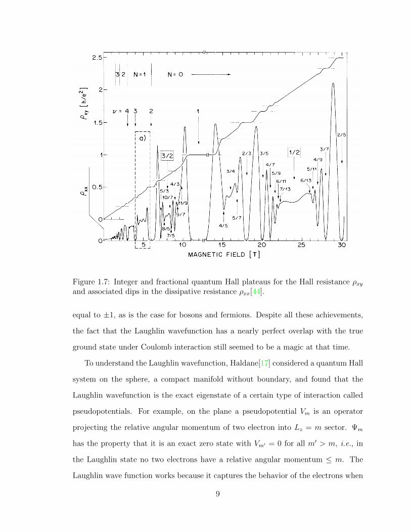
Figure 1.7: Integer and fractional quantum Hall plateaus for the Hall resistance ρxyand associated dips in the dissipative resistance ρxx[44].
equal to ±1, as is the case for bosons and fermions. Despite all these achievements,
the fact that the Laughlin wavefunction has a nearly perfect overlap with the true
ground state under Coulomb interaction still seemed to be a magic at that time.
To understand the Laughlin wavefunction, Haldane[17] considered a quantum Hall
system on the sphere, a compact manifold without boundary, and found that the
Laughlin wavefunction is the exact eigenstate of a certain type of interaction called
pseudopotentials. For example, on the plane a pseudopotential Vm is an operator
projecting the relative angular momentum of two electron into Lz = m sector. Ψm
has the property that it is an exact zero state with Vm′ = 0 for all m′ > m, i.e., in
the Laughlin state no two electrons have a relative angular momentum ≤ m. The
Laughlin wave function works because it captures the behavior of the electrons when
9

they come close to each other. In other words, the FQHE is governed by the short-
range part of the Coulomb interaction. In the same paper, Haldane also proposed
a scheme for constructing a hierarchy of quantum Hall states at different fillings by
proliferating the quasiholes or quasiparticles. For example, a quasiparticle in the 1/3
state can be viewed as a 2/5 droplet surrounded by all the other 1/3 droplets where
a p/q droplet contains p electrons and q flux quanta. A similar construction was also
proposed by Halperin[22]. The composite-fermion approach proposed by Jain is also
an alternative to generate quantum Hall states[25].
The construction of neutral excitations came with the seminal paper by Girvin,
Macdonald and Platzman[13]. The technique used there is closely analogous to Feyn-
man’s theory of superfluid helium. The neutral excitation is created by acting ρq, the
density operator in the momentum space, on the ground state. The expression for
the energy of the excitation is
E(q) =O(q4l4)
S(ql), (1.5)
where S(ql) is the static structure factor. This is called the magneto-roton mode and
Fig.(1.2) shows the structure factor of 1/3 and 1/5 fillings. The peak of the structure
factor gives rise to the minimum of the mode called the roton-minimum. At small
q, the structure factors goes as q4 so there is a finite gap at long wave length. The
ripples at large q will become increasingly violent as the filling factor gets smaller
signifying a possible phase transition to a periodic Wigner crystal[9].
Apart from the Laughlin series and the hierarchy series, there exist other types of
quantum hall states. In their paper, Moore and Read[31] pointed out that the Laugh-
lin wavefunctions were mathematical related to conformal blocks of 2D conformal field
10

Figure 1.8: Static structure factor for Laughlin 1/3 state and 1/5 state. Solid lineis modified-hypernetted-chain calculation. Dashed line is from fit to Monte Carlodata[13]. The peak of the structure factor gives rise to a roton-minimum at finitewave vector in the magneto-roton mode.
theory. They used this observation to construct a state in the form of
ΨMR = Pfaff
(1
zi − zj
)∏i<j
(zi − zj)2e−12
∑i |zi|2 , (1.6)
where the Pfaffian is defined by
Pfaff(Mij) =1
2N/2(N/2)!
∑σ∈SN
sgnσ
N/2∏k=1
Mσ(2k−1),σ(2k) (1.7)
with SN being the permutation group. It is now called the Moore-Read state and
is a candidate for the ground state of 5/2 filling (1/2 filling in the second Landau
level). An amazing property of this state is that it possesses excitations that obey
11

Figure 1.9: Order of slater determinants in the expansion of Laughlin 1/3 state with 3electrons. The root configuration is 1001001, which is always the highest in order, andeach Slater determinant corresponds to a partition (in this case of 10) by transcribingthe position of each electron. The order of the partitions is determined by comparingthe positions from left to right. The lower states can be obtained from squeezing twoelectrons closer to each other from higher states.
non-abelian braiding statistics[6]. They are building blocks of topological quantum
computing[33]. The Read-Rezayi series are even more complicated states[37].
Notice that the model wavefunctions are all written in the first-quantized language.
To transform them into the second-quantized language, i.e., as an expansion in Fock
basis (Slater determinants for fermionic systems) is not straightforward. Bernevig and
Haldane[4] observed that the bosonic version of these model wavefunctions, for both
the ground states and the excitations, were Jack polynomials. These polynomials
are homogeneous and symmetric, constructed from a partition λ (called the “root
configuration”) and a parameter α. Each partition corresponds to a basis state in the
Fock space and only those basis states that are lower in the order compared to the
root configuration can appear in the expansion, where the order is defined by that
of the partition. Fig.(1.9) shows an example. The coefficients of the expansion have
a recursive relation that depends on α, which facilitates numerical generation of the
wavefunctions. Model wavefunctions for neutral excitations constructed with Jack
polynomials were proposed in Ref[45]. The interpretation of the neutral excitations
is that (at least at large q) they are dipole moments formed by a quasiparticle and a
quasihole. See Fig.(1.10).
The jack polynomials are still exact model wavefunctions while the matrix-
product-state (MPS) representation[47] is a useful approximation of the model
12

Figure 1.10: Root configurations of model wavefunctions for neutral excitations forthe Langhlin 1/3 system. The total angular momentum L is calculated with respectto the ground state (with root configuration 1001001 · · · 1001). Note the smallest Lthat can be created is 2. The black dots indicate the positions of quasiparticles whilethe white dots those of quasiholes. They are determined by counting the numberof electrons in three consecutive orbitals. When L increases, the excitation can beroughly viewed as a pair of quasihole and quasiparticle that forms a dipole moment.
wavefunctions that further enables numerical calculations of various properties of
the FQHE. This is closely related to the concept of entanglement spectrum that
was introduced by Li and Haldane[30]. The universality within the entanglement
spectrum of the model wavefunctions are closely related to the fact that they are
identical to conformal blocks of a “bulk CFT” and that the cut that divides the
system into two parts mimics the physical edge where an “edge CFT” describes the
gapless edge excitations, which is investigated by Wen[42].
At first sight the models wavefunctions appear to be rigid in the sense that they
contain no variational parameters. In a geometric description of the FQHE initiated
by Haldane[19], a hidden degree of freedom called the guiding-center metric that de-
fines the shape of the “correlation hole” around an electron can be tuned to minimize
the Coulomb energy. This is numerically done in Ref[46]. Also the zero fluctuation
of this metric gives rise to the gap at zero momentum. This metric is a dynamic
quantity that has nothing to do with that of the underlying manifold. A metric of
13

free choice will be a critical concept in the generic theory for the IQHE presented in
this thesis.
1.3 Continuous model
In this section we want to review the usual Galilean-invariant continuous model to
illustrate some basic concepts and prepare the reader for later (more generic) discus-
sions. Consider a 2DEG living on the infinite 2D Euclidean plane under a uniform
magnetic field B. The dispersion is quadratic, i.e., the Hamiltonian is in the form of
H =1
2m
(p2x + p2y
), px,y = −i~∂x,y − eAx,y. (1.8)
We will use the so-called symmetry gauge Ax = 12By and Ay = −1
2Bx. The commu-
tator of the momentum operators has a simple form,
[px, py] = i~eB, (1.9)
which is reminiscent of the canonical commutator [x, px] = i~. Indeed, we can build
ladder operators out of the momentum operators by
a =px + ipy√
2~eB, a† =
px − ipy√2~eB
, (1.10)
so that [a, a†] = 1. The Hamiltonian is then
H = ~ωc(a†a+ 12), ωc = eB/m. (1.11)
The spectrum is thus equivalent to that of a harmonic oscillator
En = ~ωc(n+ 12), (1.12)
14
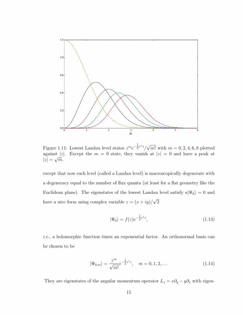
Figure 1.11: Lowest Landau level states zme−12z∗z/√m! with m = 0, 2, 4, 6, 8 plotted
against |z|. Except the m = 0 state, they vanish at |z| = 0 and have a peak at|z| =
√m.
except that now each level (called a Landau level) is macroscopically degenerate with
a degeneracy equal to the number of flux quanta (at least for a flat geometry like the
Euclidean plane). The eigenstates of the lowest Landau level satisfy a|Ψ0〉 = 0 and
have a nice form using complex variable z = (x+ iy)/√
2
|Ψ0〉 = f(z)e−12z∗z, (1.13)
i.e., a holomorphic function times an exponential factor. An orthonormal basis can
be chosen to be
|Ψ0,m〉 =zm√m!e−
12z∗z, m = 0, 1, 2, . . . (1.14)
They are eigenstates of the angular momentum operator Lz = x∂y − y∂x with eigen-
15

Figure 1.12: Landau levels under a rotationally invariant confining potential. TheFermi energy EF is between the 2nd and the 3rd Landau levels and has three inter-sections with the lowest three Landau levels. Theses intersections correspond to threebranches of gapless edge modes.
value m. Notice that the peak of |Ψ0,m| is at |z| =√m (see Fig.(1.11)) so if we add a
rotationally invariant confining potential that increases monotonically with |z| then
we will have a spectrum where (in each Landau level) energy increases with angular
momentum index. See Fig. (1.12). Then if we set the Fermi energy just above the
nth Landau level, it will have n intersections with the lowest n bands, creating n
gapless edge modes.
We want to look at in particular |Ψ0,0〉 = e−12z∗z, which is a coherent state centered
at the origin. If we “raise” the state using a† we will have a series of states
(a†)k|Ψ0,0〉 = (z∗)ke−12z∗z. (1.15)
16

These can be called coherent states in the kth Landau level. In the next chapter we
will see that a coherent state (in any Landau level) will have a generic form
f(z∗)e−12z∗z (1.16)
in the absence of Galilean or rotational symmetry.
1.4 Galilean and rotational symmetries
In the previous section we modeled the IQHE using a quadratic Hamiltonian with
Euclidean metric. That Hamiltonian has both Galilean and rotational symmetries.
A general Galilean-invariant Hamiltonian is
H =1
2mabpapb, (1.17)
where mab is the inverse mass tensor inherited from the band structure. A general
rotationally invariant Hamiltonian is
H =K∑k=1
ck(gabpapb
)k, (1.18)
where the metric is the same for every term. A Hamiltonian in this form can still be
exactly diagonalized using the same technique as in the Galilean invariant case. It’s
just that the energy levels are not evenly separated.
There has been recent interest in geometrical properties of the QHE[7, 8, 1, 15,
10, 11, 16, 38]. A typical field-theoretical model that is used in the literature is
S =
∫d2xdt
√g
[i
2~ψ†∂0ψ −
i
2~(∂0ψ
†)ψ + eA0ψ†ψ − ~2
2mgij(Diψ)†Djψ +
gsB
4mψ†ψ
],
(1.19)
17

which clearly has Galilean symmetry. The Newton-Cartan geometry proposed in
Ref.[38] is also a generalization of the Galilean symmetry. However, these are not
generic symmetries for electrons moving in a crystal background and can only be
viewed as a lowest order expansion of the band structure around a band minimum.
A simple toy model is certainly useful in revealing the basic properties of the QHE,
especially the topological ones since they are, by nature, not related to the presence
or absence of symmetries and a simple model offers an easy way to calculate them.
However, for geometrical properties of the QHE the use of special symmetries might
obscure fine structures in the system and thus can be potentially misleading. We
would like to overcome this obstacle in understanding the IQHE.
1.5 Road map
The purpose of this thesis is to present a generic theory of the IQHE in the absence
of Galilean or rotational symmetry. Preparatory material discussing the algebra of
Landau orbits and guiding centers is provided in Chap.(2). There we also construct
guiding-center coherent states that will be studied in detail later. After that we will
achieve two goals. The first is to properly characterize the coherent state in each
Landau level, which is done numerically in Chap.(3) for a quartic Hamiltonian. A
topological quantity called the topological spin will be introduced there by investi-
gating the root distribution of the antiholomorphic part of the coherent states. The
second goal is to clarify distinct geometrical properties for the IQHE. In Chap.(4) a
generic formula for the Hall viscosity, response to a non-uniform flow velocity field,
will be derived and compared to previous results in the literature. In Chap.(5) we
will calculate generic electromagnetic responses and differentiate between universal
terms that are diagonal in the Landau levels and non-universal terms that depend on
inter-Landau-level mixing. Conclusions can be found in Chap.(6).
18

Chapter 2
A generic approach
Since we want to forfeit Galilean and rotational symmetries, we need a generic ap-
proach to address the IQHE problem. We will first introduce the algebra of Landau
orbits and guiding centers, two independent degrees of freedom. They both possess
a metric of free choice. Then we will define the guiding-center coherent states by
providing a natural choice for the guiding-center metric. After presenting a generic
form of the single-particle Hamiltonian we will look closely at the quartic case, which
will be studied in detail numerically in the next chapter.
2.1 The algebra of Landau orbits and guiding cen-
ters
As mentioned in Sec.(1.3), the 2D dynamic momentum operator is defined as
pa = −i~∂a − eAa(x), (2.1)
19

with the commutator being
[pa, pb] = i~eεabB(x). (2.2)
We have used the fact that
∂aAb − ∂bAa = B(x)εab (2.3)
which is true regardless of gauge choice. We will focus on the case of a uniform
magnetic field B(x) = B and leave perturbations to Chap.(5) where we discuss elec-
tromagnetic response functions. Now decompose the electron coordinate as follows,
xa = Ra + Ra, (2.4)
Ra ≡ (eB)−1εabpb, (2.5)
where Ra is the “guiding-center” coordinate and Ra is the Landau-orbit coordinate.
The physical interpretation of this decomposition is that the guiding-center coordinate
describes the position of the center of the orbit with respect to the origin while the
Landau-level coordinate describes the relative position of the electron to the orbit
center, as shown in Fig.(2.1). An amazing property of this decomposition is that the
two parts are independent degrees of freedom, i.e.,
[Ra, Rb] = 0. (2.6)
20

Figure 2.1: Landau-orbit coordinate R and guiding-center coordinate R.
However these coordinates are not classical quantities, i.e., they have non-trivial
commutators,
[Ra, Rb] = −i~(eB)−1εab, (2.7)
[Ra, Rb] = i~(eB)−1εab, (2.8)
and thus can not be diagonalized simultaneously, unlike the usual coordinate opera-
tors in the Schrodinger picture where x|x〉 = x|x〉. The best we can do is to construct
a coherent state that is physically a fuzzy object saturating Heisenberg’s uncertainty
principle, which is detailed in the next section. Also notice that the commutators have
opposite signs, which is another manifestation of the opposite chiralities of Landau
orbits and edge states (guiding-center flow) mentioned in Sec.(1.1).
21

We can define two sets of harmonic-oscillator operators for Landau-orbit and
guiding-center degrees of freedom respectively,
a =
√eB
2~eaR
a, b =
√eB
2~eaR
a, (2.9)
a† =
√eB
2~e∗aR
a, b† =
√eB
2~e∗aR
a, (2.10)
where the ea, called (complex 2D) frame fields, satisfy
εabe∗aeb = εabe∗aeb = i, (2.11)
so that the harmonic-oscillator operators have the expected commutation relations
[a, a†] = [b, b†] = 1, [a, b] = [a, b†] = 0. This fixes the antisymmetric part of eaeb and
we can define a metric from the symmetric part for both Landau-orbit and guiding-
center sectors,
gab = e∗aeb + e∗b ea, gab = e∗aeb + e∗b ea. (2.12)
These metrics are unimodular meaning that the determinant
det g = 12εacεbdgabgcd (2.13)
is 1. The inverse metrics are then
gab = εacεbdgcd, gab = εacεbdgcd. (2.14)
22

Figure 2.2: Schematic drawing of the effect of three area-preserving generators γ22,γ11, and γ12. γ22 and γ11 translate one of the two momentum operators while γ12 is arotation.
Up until now we have not specified the frame fields or the metrics. In fact different
choices are related by Bogliubov transformations
a′
a′†
=
eiφ1 cosh θ eiφ2 sinh θ
e−iφ2 sinh θ e−iφ1 cosh θ
a
a†
(2.15)
parametrized by three parameters φ1, φ2 and θ. This can also be viewed from the
perspective of area-preserving deformations of the momentum-space
pa → U(β)paU(β)−1. (2.16)
The unitary operator U(β) is defined as
U(β) = exp(iπβabγab), (2.17)
γab = (4~eB)−1{pa, pb}, (2.18)
23

where βab is a real symmetric matrix. The action of the generators can be understood
by calculating their commutators with the momentum operators
[pa, γbc] = 12i(εabpc + εacpb). (2.19)
We can see that γ11 leaves p1 invariant while translates p2 in the direction of p1. γ22
acts in a similar way and γ12 corresponds to a rotation, as illustrated in Fig. (2.2).
These generators obey a Lie-algebra
[γab, γcd] = 12i(εacγbd + εbcγad + εadγbc + εbdγac) (2.20)
that will be useful in deriving the Hall viscosity in Sec. (4.3).
If the system under study has rotational symmetry, it’s natural to identify the
two metrics, then the z-component of the angular momentum operator written as
Lz = b†b− a†a = b†b+ 12− (a†a+ 1
2) (2.21)
is a good quantum number. We have a finer structure of the spectrum now by realizing
that in nth Landau level the smallest Lz is −n, as illustrated in Fig.(2.3).
The differentiation between two independent and fundamentally arbitrary metrics
is critical in our generic description for the IQHE without Galilean or rotational
symmetry. In the next section we will introduce what we think is the most natural
choice for the guiding-center metric in the process of defining guiding-center coherent
states.
24

Figure 2.3: Sketch of the single-particle spectrum for a rotationally invariant quantumHall system. The z-component of the angular momentum Lz = b†b − a†a is a goodquantum number and the lowest Lz for the nth Landau level is −n. a† raises a stateto the next Landau level and lowers Lz by 1 while b† raises a state to the next Lzeigenstate within the same Landau level.
2.2 Guiding-center coherent states
We said at the end of the introductory chapter that we wanted to characterize the
eigenstates at the absence of rotational symmetry. Since a Landau level is macroscop-
ically degenerate (this is due to the existence of two independent sets of algebra), we
need to look at a specific state in each Landau level and a coherent state would be a
good candidate. Then comes the problem of how to construct these coherent states.
We inherit the spirit of a usual coherent state, which is the closest quantum
mechanical state to the classical state, and define here a guiding-center coherent
state with a fixed guiding center
〈Ψn(x, g)|R|〈Ψn(x, g)〉 = x (2.22)
25

Figure 2.4: A coherent state on the guiding-center plane (analogous to the phasespace of a harmonic oscillator). The coordinates of the center of the coherent stateindicate the expectation values of the guiding-center operators. The shape of thecoherent state is determined by the guiding-center metric and the area of the fuzzyregion is πl2B. The combination of this uncertainty with that of the Landau orbits,also πl2B, gives the area per flux quantum 2πl2B.
that satisfies
gab(〈Ψ|RaRb|Ψ〉 − 〈Ψ|Ra|Ψ〉〈Ψ|Rb|Ψ〉) =~eB≡ l2B, (2.23)
i.e., the guiding-center part saturates Heisenberg’s uncertainty principle as an equal-
ity. Fig.(2.4) illustrates such a coherent state on the guiding-center plane (similar to
the phase space of a harmonic oscillator). Without loss of generality, we will only
consider the case x = 0, a coherent state centered at the origin. Notice that the
coherent state explicitly depends on the guiding-center metric and different choices
of the metric correspond to physically distinct states. It turns out that there is a
“natural” choice for each Landau level that is proportional to the expectation value
26
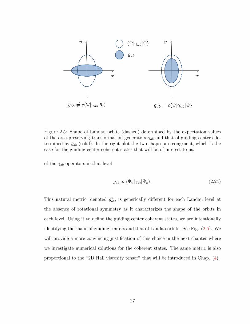
Figure 2.5: Shape of Landau orbits (dashed) determined by the expectation valuesof the area-preserving transformation generators γab and that of guiding centers de-termined by gab (solid). In the right plot the two shapes are congruent, which is thecase for the guiding-center coherent states that will be of interest to us.
of the γab operators in that level
gab ∝ 〈Ψn|γab|Ψn〉. (2.24)
This natural metric, denoted gnab, is generically different for each Landau level at
the absence of rotational symmetry as it characterizes the shape of the orbits in
each level. Using it to define the guiding-center coherent states, we are intentionally
identifying the shape of guiding centers and that of Landau orbits. See Fig. (2.5). We
will provide a more convincing justification of this choice in the next chapter where
we investigate numerical solutions for the coherent states. The same metric is also
proportional to the “2D Hall viscosity tensor” that will be introduced in Chap. (4).
27

We can obtain a more explicit expression for the coherent states by defining a
complex structure on the 2D Euclidean plane
z = eaxa/(√
2lB), (2.25)
and picking a “symmetric” gauge for the vector potential
Aa(x) =1√2i(z∗ea − ze∗a). (2.26)
This gauge is more generic in the sense that it contains an arbitrary field ea that goes
hand in hand with the guiding-center metric gab. Notice that when e = (1, i)/√
2 we
go back to the usual symmetric gauge introduced in Sec.(1.3). Now the guiding-center
harmonic-oscillator operators have explicit expressions
b = 12z∗ + ∂z, b† = 1
2z − ∂z∗ . (2.27)
We use an alternative definition of a coherent state (centered at the origin)
b|Ψn〉 = 0 (2.28)
to obtain a generic form
Ψn(z, z∗) = fn(z∗)e−12z∗z, (2.29)
where the metric dependence is implicit in the definition of z. We see that it is
an anti-holomorphic function times an exponential part. This is quite reminiscent
(but should be differentiated from) the well-known property of lowest Landau level
wavefunctions (a holomorphic function times an exponential factor) mentioned in Sec.
(1.3) .
28

2.3 A generic Hamiltonian
In Sec.(1.4) we clarified what we meant by Galilean and rotational symmetries for a
single-particle Hamiltonian. Now we will introduce a generic Hamiltonian in terms
of the momentum operators
H(p) =n∑k=1
1
(2k)!Ha1a2...a2kpa1pa2 . . . pa2k , (2.30)
where the coefficients Ha1a2...a2k are fully symmetric in the indices. The Hamiltonian
contains only even order terms and has inversion symmetry
H(p) = H(−p). (2.31)
For an arbitrary function f(p) to be well-defined when the two variables pa are non-
commuting, it should be an entire function meaning that for any c-number p0, f(p0+
(p− p0)) expanded in powers of δp = p− p0
f(p) =∞∑n=0
fa1a2...an(p0){δpa1 , . . . , δpan}, (2.32)
where {. . . } is a symmetrized product, is absolutely convergent. The Hamiltonian
defined here is a polynomial in pa so the condition is always satisfied. For it to be
bounded below, the coefficient for the highest term needs to be positive semi-definite,
i.e.,
Aa1a2...a2npa1pa2 . . . pa2n ≥ 0 (2.33)
for all p 6= 0. But we will impose a stricter condition here that for all p 6= 0, ε(λp),
the classical version of H(λp) by treating p as a c-number, is strictly monotonically
increasing for 0 ≤ λ <∞ and unbounded as λ→∞. This constraint guarantees that
29

Figure 2.6: Semiclassical quantization of Landau orbits. The semiclassical orbits areclosed equipotential lines of the dispersion relation ε(p) and the area enclosed by theorbit is quantized according to A(En) = 2π~eB(n+ 1
2).
any curve determined by the equation ε(p) = E > ε(0) is topologically equivalent
to a circle S1 that encloses the origin. The curves are actually classical orbits as the
equations of motion are
dxa
dt=
∂ε
∂pa≡ va,
dpadt
= eBεabvb, (2.34)
so the change in p is always perpendicular to the gradient field v. Bohr-Sommerfeld
quantization can be applied so the area enclosed by these curves are quantized as
A(En) = 2π~eB(n+ 12), (2.35)
and the corresponding En are the Landau level energies. See Fig. (2.6). This will be
revisited for numerical solutions in the next chapter.
30

To diagonalize the Hamiltonian, we still need to transform the momentum opera-
tors to harmonic-oscillator operators a and a†. When rotational symmetry is absent,
there is no “best” choice of the metric gab that puts the Hamiltonian in a readily
diagonalizable form. However, since we introduced a natural metric for the guiding-
center coherent states defined in the last section, using the same metric for gab will
make a and a† expressible with the same complex structure z as
a = 12z + ∂z∗ , a† = 1
2z∗ − ∂z, (2.36)
and a coherent state that is also an eigenstate of a†a with eigenvalue n is
Ψ0n =
(z∗)n√n!e−
12z∗z. (2.37)
Thus a coherent state in the nth Landau level Ψn as an expansion in the Ψ0n, a result
of diagonalizing the Hamiltonian, can be readily expressed as a Taylor expansion in
terms of z∗, i.e.,
Ψn =∞∑k=0
ckΨ0k =
∞∑k=0
ck(z∗)k√k!e−
12z∗z, (2.38)
which is a clean form for further investigation. In the next chapter we will employ
numerical methods to diagonalize the Hamiltonian and obtain the expansion with a
cutoff on the number of available Ψ0n.
31

2.4 The quartic case
From now on we will focus on the simplest non-trivial case where the Hamiltonian
only has quadratic and quartic terms, i.e.,
H = Aab1 papb + Aabcd2 papbpcpd. (2.39)
Let’s look at the quartic term. If we treat the components of p as classical variables,
Aabcd2 papbpcpd is then a homogeneous polynomial of degree four and can be trans-
formed into a univariate polynomial of p1/p2. This polynomial can have: I) two pairs
of complex conjugate roots, II) one pair of complex conjugate roots and a real root
of multiplicity 2, III) two real roots each of multiplicity 2, and IV) one real root of
multiplicity 4. The existence of a pair of complex conjugate roots means the corre-
sponding quadratic form is positive-definite and therefore the coefficient matrix can
be interpreted as a metric. Based on this consideration, those four cases correspond
to four different classes (labeled by Roman numerals) of the quartic term
Aab,cd2,I = gab1 gcd2 + gab2 g
cd1 ,
12(gab1 + gab2 ) = cgab0 , (2.40)
Aab,cd2,II = gab1 uc1u
d1 + ua1u
b1gcd1 , (2.41)
Aab,cd2,III = ua1ub1u
c2u
d2 + ua2u
b2u
c1u
d1, u
a1u
b1 + ua2u
b2 = λgab0 , (2.42)
Aab,cd2,IV = ua1ub1u
c1u
d1, (2.43)
where λ > 0, and c ≥ 1. The contour plots in the momentum space for a typical
member in each class is plotted in Fig.(2.7). It can be seen that only class I has
closed contours so it will be our main focus. There are two metrics gab1 and gab2 in the
definition. After a SL(2, R) transformation, as illustrated in Fig.(2.8), we can put
32

Figure 2.7: Contour plots in the momentum space of a typical member in each classof the quartic term. The quartic terms are I) {5p21 + p22, p
21 + 5p22}, II) {p21, p21 + p22},
III) {p21, p22} and IV) p41. Notice that only the contours for class I are closed.
33

Figure 2.8: Sketch of creating C4 symmetry under a SL(2, R) transformation. Start-ing from gab1 = δab (which can always be achieved under a certain basis), a rotationcan put gab2 into a diagonal form. Then a scaling of one axis can put the two metricsinto the final configuration where gab1 and gab2 are both diagonal and related by a 90degree rotation.
these two metrics in the form
gab1 =
d1 0
0 d2
, gab2 =
d2 0
0 d1
. (2.44)
This is indeed the case for the example provided in Fig.(2.7). The quartic term is
then
H = E0
((γ11 + γ22)
2 + (c− 1){γ11, γ22}). (2.45)
This form has an explicit C4 symmetry under (p1, p2) → (−p2, p1) or γ11 ↔ γ22.
However we should remark that this C4 symmetry is only possessed by a pure quartic
term and has no generic significance.
34

Chapter 3
Numerics
In the previous chapter we introduced a generic form of the single-particle Hamil-
tonian and looked closely at the quartic case. Unfortunately we were not able to
diagonalize the Hamiltonian analytically, so in this chapter we will employ numerical
methods. By imposing a cutoff on the number of available basis states we transform
the problem into matrix diagonalization. After we obtain the eigenstates, which are
in the form of a polynomial in z∗ times a exponential factor, we will look at the root
distribution of that polynomial and define a “topological spin” sn = n+ 12
where n is
the number of the central roots separated from the outer roots by the semiclassical
orbit. Its connection to the “shift” will be explained. At the end of this chapter
we will briefly talk about Nevanlinna theory that studies the zero distribution and
growth rate for solutions of complex differential equations.
3.1 Algorithm
The major steps of the algorithm are shown in Fig.(3.1). In Eq.(2.24) we have specified
the guiding-center metric for the coherent states to be the expectation values of γab.
However, before we diagonalize the Hamiltonian and obtain the eigenstates, we don’t
have that metric at hand. Nonetheless, diagonalization only requires specifying the
35

Landau-orbit metric and the choice doesn’t affect the results (at least when there is no
cutoff). Therefore as a first step, we pick the Euclidean metric δab to define Landau-
orbit harmonic-oscillator operators a and a†. After calculating the expectation values
of γab in a certain Landau level indexed by n, we re-define a and a† using that natural
metric gnab and re-diagonalize the Hamiltonian under the new basis (eigenstates of
a†a). To obtain the frame fields, use
ea = gabeb = iεabe
b, (3.1)
or in matrix form (letting ea ∝ (1, α))
g11 g12
g21 g22
1
α
=
0 i
−i 0
1
α
. (3.2)
We have
ea =
√g222
(1,−g12 − ig22
), (3.3)
and a = eapa/√~eB. If we define
pE1 = (a+ a†)/√
2, pE2 = −i(a− a†)/√
2, (3.4)
then the expectation value of {pEa , pEb } in the nth eigenstate should be the Euclidean
metric δab. This can be checked to make sure that the algorithm is working properly.
We then pick the nth eigenstate, whose natural metric now defines both a† and
b†. The eigenstate has a representation (with a cutoff on the available orbitals)
Ψn =N∑k=0
ck(z∗)k√k!e−
12z∗z, (3.5)
36

where ck are the components of the eigenvector and the complex structure z is asso-
ciated with the natural metric. We will investigate how the cutoff might affect the
eigenstate.
Since the eigenstate is represented as an antiholomorphic polynomial completely
determined by its roots, our idea is to characterize the eigenstate from the perspective
of the distribution of its roots on the complex plane. The algorithm that is used to
find the roots is called Jenkins-Traub algorithm[35]. The basic idea is as follows.
Consider a polynomial
P (z) = zn + an−1zn−1 + · · ·+ a1z + a0 =
p∏j=1
(z − αj)mj (3.6)
where the ai are complex numbers with a0 6= 0. The zero αj has multiplicity mj, j =
1, . . . , p so that∑p
j=1mj = n. We have
P ′(z) =
p∑j=1
mjPj(z), (3.7)
Pj(z) =P (z)
z − αj. (3.8)
Generate a sequence of polynomials H(λ)(z) starting with H(0)(z) = P ′(z), each of
the form
H(λ)(z) =
p∑j=1
c(λ)j Pj(z), (3.9)
and the goal is to let H(λ)(z)→ c(λ)1 P1(z), then a sequence {tλ}
tλ+1 = sλ −P (sλ)
H(λ+1)(sλ), (3.10)
H(λ)(z) =H(λ)(z)∑pj=1 c
(λ)j
, (3.11)
37

Figure 3.1: Diagram of numerical procedures. The Hamiltonian is diagonalized withthe Landau-orbit metric identical to the Euclidean metric. After the natural metricfor a specific Landau level indexed by n is calculated, diagonalize the Hamiltonian fora second time using that metric to define a and a†. The roots of the polynomial part ofthe nth eigenstate (which is in nth Landau level) are then found using Jenkins-Traubalgorithm. For another Landau level n′ 6= n, restart from the second step.
where sλ is an arbitrary sequence, approaches sλ − (sλ − α1) = α1. The H(λ)(z) are
generated by the formula
H(λ+1)(zλ) =1
z − sλ
(H(λ)(z)− H(λ)(sλ)
P (sλ)P (z)
)(3.12)
=P (z)
z − sλ
p∑j=1
c(λ)j
(1
z − αj− 1
sλ − αj
)
=
p∑j=1
c(λ)j
αj − sλPj(z). (3.13)
If we choose sλ so that it approaches α1 (e.g., let sλ = tλ) we will achieve our goal.
38

A practical problem in the process described above is that the factor 1/√k! present
in Eq.(3.5) decays so fast that at k ∼ 170 it already reaches the limit of double-
precision floating-point format. To achieve a higher cutoff, we used the arbitrary-
precision data type provided by the GMP library in the root-finding algorithm.
We also needed to transform the LAPACK routines used for diagonalization into
arbitrary-precision versions and we found an open-source package called MPACK[32]
that suited our purpose.
3.2 Topological spin
In this section we will present numerical results, particularly the distribution of com-
plex roots for a guiding-center coherent state. An important concept dubbed a topo-
logical spin will be introduced to characterize different Landau levels.
Before jumping into the details, let’s get some taste from a benchmark case where
we calculate the roots of an expansion of the modified Bessel function of the first kind
I0(2z) =N∑k=0
1
(k!)2z2k. (3.14)
To mimic the C4 symmetry of a pure quartic term, we will use I0(2z2) instead. The
function I0(z) has inversion symmetry I0(z) = I0(−z) and all its zeros lie on the imag-
inary axis. Therefore the zeros of I0(2z2) should be aligned on four rays emanating
from the origin with arguments ±π/4 and ±3π/4. Fig.(3.2) verifies this (along with
numerical artifacts).
We will start with class I quartic case (for the definition of the four classes, see
Sec.(2.4)). A typical layout of the roots is presented in Fig.(3.3). The central zeros
are organized in a cross shape due to the C4 symmetry. There are n mod 4 degenerate
roots at the origin where n is the Landau-level index, and the degeneracy will be lifted
once we add quadratic terms to the Hamiltonian (as the C4 symmetry is broken). The
39

Figure 3.2: Roots of an expansion of I0(2z2) at cutoff N = 500. The four rays of
roots at arguments ±π/4 and ±3π/4 are true roots while the arcs on the outside aredue to a finite cutoff and will be pushed further outward when the cutoff increases.
feature that also appears in the benchmark case is the presence of four “spikes” that
point to the origin at ±45 and ±135 degrees. The new features are the regions with
quasi-uniform 2D distributions bounded by lines of roots also with nearly constant
density. The precise locations of the roots inside those 2D regions are sensitive to
perturbation of the Hamiltonian, but we believe the very existence of such “dark”
areas is universal.
Note that there are also truncation-dependent features tied to the boundary
|z| ≈ RN , where N is the cutoff, but the structure for |z| � RN becomes inde-
pendent of N as it, and consequently RN , is increased, as illustrated in Fig.(3.4). We
40

−40 −20 0 20 40
−40
−20
0
20
40
Figure 3.3: Root distribution on the complex plane of the coherent state in the 10thLandau level for class I quartic term in Eq.(2.45) with c−1 = 4 at a truncation of 500even-parity states. Ten central zeros, with two being degenerate at the origin, forma cross due to the C4 symmetry. The peripheral zeros also have interesting features,such as four “spikes” pointing to the origin and line charges with constant densitythat bound 2D regions of quasi-uniform distributions. The arcs on the boundary aregenerated due to finite truncation and should not be regarded as part of the zeropattern.
41
−60 −40 −20 0 20 40 60−60
−40
−20
0
20
40
60
N 500 7501000
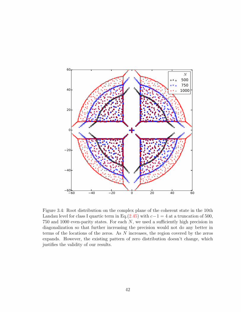
Figure 3.4: Root distribution on the complex plane of the coherent state in the 10thLandau level for class I quartic term in Eq.(2.45) with c−1 = 4 at a truncation of 500,750 and 1000 even-parity states. For each N , we used a sufficiently high precision indiagonalization so that further increasing the precision would not do any better interms of the locations of the zeros. As N increases, the region covered by the zerosexpands. However, the existing pattern of zero distribution doesn’t change, whichjustifies the validity of our results.
42

therefore believe that this calculational method reveals the true structure of roots
of the antiholomorphic non-polynomial function fn(z∗) in a range |z| < R that can
be increased at will at the expense of increasing the floating-point precision of the
numerical diagonalization.
Let’s now look at other features of the distribution. There is a 2D electrostatic
analogy by interpreting
ln |Ψn|2 = 2N∑k=0
ln |z − zk| − z∗z + const., (3.15)
where zk are the roots, as the Coulomb potential at z of a 2D distribution of charges
located at the roots and a neutralizing background charge density 1/π (if each root
carries a unit charge). To visualize that, we show in Fig.(3.5) the contours of ln |Ψn|2.
We see piecewise segments with different curvatures as the 2D regions change effective
background charge density and the linear alignments of roots act as branch cuts.
Notice the “volcano crater” at the center enclosed by an annulus-like region containing
local maxima and saddle points. The free parameter c− 1 controls the shape of the
annulus. A simple calculation reveals that c− 1 > 2 corresponds to a concave shape,
while c− 1 < 2 convex. This annulus is a fattened version of the semiclassical orbit.
Actually if we define a “ridge” inside the annulus as the boundary between two regions
where the gradient field flows toward either the origin or infinity (the local maxima
and the saddle points are all right on the boundary), as shown in Fig. (3.6), we find
that the area enclosed by that ridge is exactly πn with n being the Landau level
index, which corresponds to an area of 2π~eBn on the momentum plane. This is just
the Bohr-Sommerfeld quantization mentioned in Sec.(2.3) shifted by a constant.
To obtain an intuitive understanding of the structure, recall that in the rotation-
ally invariant case, Ψn ∝ (z∗)n exp(−12z∗z) has n zeros at the origin, a ring of maxima
at a radius of√n and a Gaussian tail extending to infinity. With a moderate per-
43

−20 −15 −10 −5 0 5 10 15 20−20
−15
−10
−5
0
5
10
15
20
−20 −15 −10 −5 0 5 10 15 20−20
−15
−10
−5
0
5
10
15
20
Figure 3.5: Contour plots of ln |Ψ10(z, z∗)|2 where Ψ10(z, z
∗) is the coherent state inthe 10th Landau level for class I quartic term (2.45) with c − 1 = 4 > 2 (top) andc − 1 = 1 < 2 (bottom). Both plots show piece-wise contours with the four spikesand the line charges as branch cuts. Another common feature is the existence of fourmaxima along the directions of the central cross and four saddle points along thoseof the spikes. Despite the similarities, the two plots also show qualitatively differentshapes of the semiclassical orbits. We see that c − 1 > 2 corresponds to concaveshapes while c− 1 < 2 to convex ones.
44

Figure 3.6: A “ridge” (dashed) defined as the boundary between two regions wherethe gradient field flows to the origin (inside) or infinity (outside). The roots are thoseof the coherent state in the 10th Landau level for class I quartic term with c− 1 = 2.Contours are also shown. Notice that the local maxima and the saddle points are allright on the ridge. The area enclosed by the ridge is πn, corresponding to an areaof 2π~eB on the momentum plane, which is consistent with (shifted) semiclassicalquantization.
turbation that breaks rotational invariance, the new zeros will only appear where the
original wavefunction has a small amplitude, namely, around the origin or along the
Gaussian tail separated by the peak in between which contains most of the weight of
the wave function. In Fig.(3.7) we show that the peak region can encompass as much
as 90 percent of the total weight.
The existence of a clean separation between the central zeros and the rest of the
pattern by an annulus-like region, or more rigorously a region with Euler characteristic
χ = 0, defined by |Ψn| ≥ V, V ∈ R+, is critical for our definition of a topological spin,
45

−30 −20 −10 0 10 20 30−30
−20
−10
0
10
20
30
Figure 3.7: Black region accounting for 90 percent of the total weight (probability)of |Ψ20|2, the coherent state in the 20th Landau level of the Hamiltonian p2x + p2y +2p4x + 3p4y + 4{p2x, p2y} + {px, p3y}. The annulus is bounded by contours at the samevalue of the amplitude |Ψ20| and cleanly separates the central zeros from the rest ofthe structure.
which is
sn = n+ 12
(3.16)
where n is the number of central zeros. Now we can provide a more convincing
justification for the natural metric used to define the coherent states. If we deform
the metric, at some point the central zeros will leak out of the “crater” region and
the coherent state doesn’t have a semiclassical counterpart anymore. An example is
shown in Fig.(3.8) where the guiding-center metric is chosen to be δab even though
46

Figure 3.8: Contours of ln |Ψ10(z, z∗)|2, a coherent state in the 20th Landau level
with the guiding-center metric gab equal to the Euclidean metric δab while the naturalmetric is extremely squeezed, which can be told from the elongated distribution of thecentral roots and the contours. Those roots are no longer separated from the outerones by an annulus-like region defined by |Ψ10(z, z
∗)| > V where V is a constant.Instead, they are divided into subgroups by those local maxima.
the natural metric is in a extremely elongated shape. The central zeros can not be
enclosed by a region that meets our requirements.
Let’s briefly look at the other three classes of pure quartic term. As mentioned
in Sec.(2.4) the classical orbits for the three classes are not closed. Although the
noncommutativity of pa gives rise to effective quadratic terms for classes II and III,
thus closing the quantum orbits, we expect that a clean separation of the central zeros
cannot be achieved for any of the three classes, which is verified in Fig.(3.9).
We now combine quartic terms with quadratic terms. We adopt a different
parametrization here
H =Ap2x +Bp2y + Cp4x +Dp4y
+ E{p2x, p2y}+ F{px, p3y}+G{p3x, py}. (3.17)
The C4 symmetry generically breaks down. However, as we go to high-energy states,
the quartic terms will eventually dominate and therefore a quasi-C4 symmetry will
47
Class II Class III
−20 −10 0 10 20
−20
−10
0
10
20
−20 −10 0 10 20
−20
−10
0
10
20
Class IV
−20 −10 0 10 20
−20
−10
0
10
20
Figure 3.9: Contour plots of ln |Ψ10(z, z∗)|2 , where Ψ10(z, z
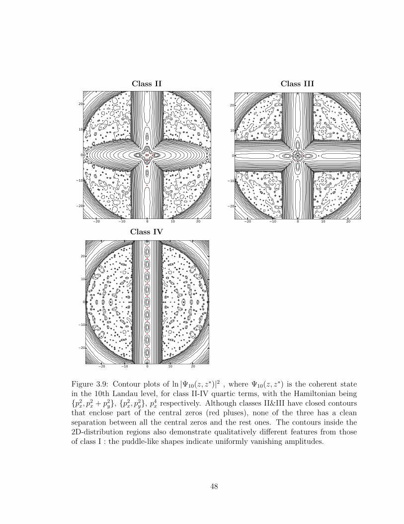
∗) is the coherent statein the 10th Landau level, for class II-IV quartic terms, with the Hamiltonian being{p2x, p2x + p2y}, {p2x, p2y}, p4x respectively. Although classes II&III have closed contoursthat enclose part of the central zeros (red pluses), none of the three has a cleanseparation between all the central zeros and the rest ones. The contours inside the2D-distribution regions also demonstrate qualitatively different features from thoseof class I : the puddle-like shapes indicate uniformly vanishing amplitudes.
48

−40 −20 0 20 40
−40
−20
0
20
40
−40 −20 0 20 40
−40
−20
0
20
40
−40 −20 0 20 40
−40
−20
0
20
40
Figure 3.10: Root distribution on the complex plane of the coherent states in the(from top to bottom) 0th, 2nd and 10th Landau level. The Hamiltonian assumes theform 20p2x + 20p2y + 2p4x + 3p4y + 4{p2x, p2y} + {px, p3y}. As the Landau level index nincreases, the C4 symmetry gradually restores as quartic terms dominate.
49
-40
-20
0
20
40
-40 -20 0 20 40
-40
-20
0
20
40
-40 -20 0 20 40
-40
-20
0
20
40
-40 -20 0 20 40
-40
-20
0
20
40
-40 -20 0 20 40
-40
-20
0
20
40
-40 -20 0 20 40
-10
-5
0
5
10
-10 -5 0 5 10-10
-5
0
5
10
-10 -5 0 5 10-10
-5
0
5
10
-10 -5 0 5 10
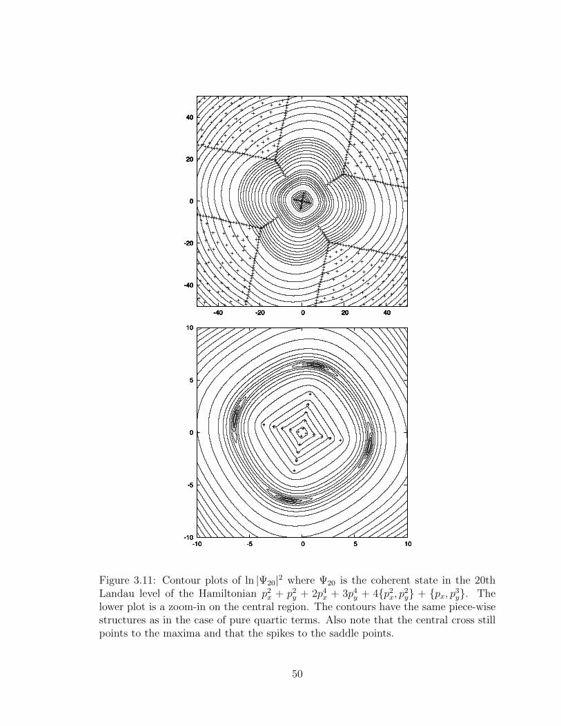
Figure 3.11: Contour plots of ln |Ψ20|2 where Ψ20 is the coherent state in the 20thLandau level of the Hamiltonian p2x + p2y + 2p4x + 3p4y + 4{p2x, p2y} + {px, p3y}. Thelower plot is a zoom-in on the central region. The contours have the same piece-wisestructures as in the case of pure quartic terms. Also note that the central cross stillpoints to the maxima and that the spikes to the saddle points.
50
gradually appear as the Landau index n increases, as shown in Fig.(3.10). Due to this
asymptotic C4 symmetry, the generic features of the root structure and the contours
still hold for a mixture of quadratic and quartic terms, as illustrated in Fig.(3.11).
To make connection with the usual Galilean theory, we remark that as we reduce
the weights of the quartic terms, the central zeros will shrink toward the origin and
the outer zeros will be pushed toward infinity (but the overall pattern doesn’t change),
consistent with the fact that at the limit of a pure quadratic term fn(z∗) becomes a
monomial (z∗)n whose roots all sit at the origin.
3.3 The “shift”
The topological spin introduced in the previous section is related to a topological
quantity called the ”shift” S that was first defined by Wen and Zee[43] in the relation
between the number of electrons Ne and the number of flux quanta Nφ on a manifold
with Euler characteristic χ,
Nφ = ν−1Ne − Sχ/2. (3.18)
The relation between the topological spin and the shift for the IQHE is
∑n
νnsn = S/2. (3.19)
The Euler characteristic is a topological invariant related to the genus, another topo-
logical invariant counting the number of ”handles” in a closed orientable 2D manifold,
by
χ = 2− 2g. (3.20)
51

Figure 3.12: Demonstration of calculation of the guiding-center spin for Laughlin 1/3state. Each composite boson is a 100 segment, and the guiding-center spin is definedas the difference between the angular momentum of a composite boson to that of auniformly distributed droplet, in this case 1
31313.
For example, a sphere has g = 0 and χ = 2, so the nth Landau level will have
2sn = 2n+ 1 extra orbitals. The exact spectrum was first calculated by Haldane[17],
who showed that the orbitals in the nth Landau level on the sphere with a charge-2S
magnetic monopole sitting at the center can be represented by a spin S + n object,
i.e., the degeneracy is 2(S + n) + 1 = 2S + (2n + 1). Another examples is the 2D
torus. It has g = 1 and χ = 0, and therefore the number of available orbitals is still
equal to Nφ. The first exact calculation was by Haldane and Rezayi[20].
For the FQHE, the shift has another contribution coming from the guiding-center
degree of freedom. The guiding-center spin is defined as the residual angular momen-
tum of a composite boson with respect to a uniform distribution of electrons. See
Fig.(3.3).
An explanation from the perspective of the effective theory is that the topological
spin couples to the Gaussian curvature of the underlying manifold and it is the total
effective curvature combining the magnetic field (U(1) curvature) and the Gaussian
curvature that determines the number of available orbitals, as illustrated in Fig.(3.3).
52

Figure 3.13: The effective curvature for a topological spin sn moving on the spherewith a Gaussian curvature Kg. The effective curvature consists of the magneticfield (curvature of U(1) gauge fields) with coupling constant e/~ and the Gaussiancurvature (curvature of the spin connection) with coupling constant sn.
The Gauss-Bonnet theorem states that
∫M
KdA = 2πχ(M), (3.21)
i.e., the integral of the Gaussian curvature K over a closed 2D manifold M is equal
to its Euler characteristic χ(M). As a result, there will be snχ extra orbitals in the
nth Landau level. However, the Gaussian curvature doesn’t need to be that of the
underlying manifold. In his geometrical description of the QHE, Haldane[19] pointed
out that even on a flat manifold there can be Gaussian curvature due to a spatially
varying guiding-center metric that minimizes local interaction.
53

We have seen that the topological spin is a well-defined topological quantity. In
the next chapter where we reformulate the Hall viscosity, we will show that the usual
identification between the scalar viscosity, a non-topological quantity, and the shift
(or equivalently the topological spin) is only a coincidence at the presence of rotational
symmetry and should not be treated as a fundamental identity.
3.4 Nevanlinna theory
In this section we would like to revisit the problem of diagonalizing the Hamiltonian
but from the perspective of solving a complex differential equation. Using the complex
representation for a and a† in Eq.(2.36) and the parametrization for the Hamiltonian
in Eq.(2.45) the eigen-problem
H|Ψ〉 = E|Ψ〉 (3.22)
can be written as a fourth order complex differential equation on the antiholomorphic
part of the wavefunction:
(∂4z∗ + α2(z∗)∂2z∗ + α1(z
∗)∂z∗ + α0(z∗))f(z∗) = 0,
α2 = −(2 +8
c− 1)z∗2,
α1 = −(4 +16
c− 1)z∗,
α0 = z∗4 − 1− 2
c− 1(1− E
E0
). (3.23)
In the mathematical literature Nevanlinna theory has been applied to the study of
global properties of solutions of complex differential equations[27]. One critical result
is that for a complex differential equation of any order with the coefficients being
entire functions of z (holomorphic functions at all finite points over the whole complex
plane), the solutions are guaranteed to be entire functions. This nice property justifies
our power-expansion method in the numerical analysis.
54

To look at the theory in more detail we need to introduce several concepts. Let f
be a meromorphic function not identically equal to 0. Let n(r, f) (the unintegrated
counting function) denote the number of roots f(z) = 0 in |z| ≤ r, each root according
to its multiplicity. We define (the counting function)
N(r, f) ≡∫ r
0
n(t, f)− n(0, f)
tdt+ n(0, f) log r, (3.24)
and (the proximity function)
m(r, f) ≡ 1
2π
∫ 2π
0
log+
∣∣∣∣ 1
f(reiϕ)
∣∣∣∣ dϕ, (3.25)
log+ α ≡ max(0, logα).
The counting function measures how the number of roots grows with r while the
proximity function calculates the average of log+ |1/f | on a circle with radius r. Then
the characteristic function is defined as
T (r, f) ≡ m(r, f) +N(r, f), (3.26)
which leads us to a very important quantity called the order of a meromorphic func-
tion,
σ(f) ≡ lim supr→∞
log T (r, f)
log r. (3.27)
If f is also an entire function, by Liouville’s theorem it is either unbounded or con-
stant. Excluding the constant case, we would generically expect m(r, f) → 0 as
r →∞ and the characteristic function is dominated by the counting function, so the
order is the exponent in the power law N(r, f) ∼ rσ. Notice that 1/f is also a mero-
morphic function, and the corresponding functions n(r, 1/f), N(r, 1/f) and T (r, 1/f)
55

can be defined. The first main theorem states that
T (r, 1/f) = T (r, f) +O(1), (3.28)
which implies that f and 1/f have the same order. For an entire function f , 1/f
doesn’t have roots at finite points, so N(r, 1/f) ≡ 0 and T (r, 1/f) ≡ m(r, 1/f). Now
the order appears in log+ |f | ∼ rσ. We see that the asymptotic growth of an entire
function is closely related to that of the number of its roots.
For an nth order complex differential equation
f (n) + an−1(z)f (n−1) + · · ·+ a1(z)f ′ + a0(z)f = 0 (3.29)
with the coefficients being entire functions, the possible orders for the solutions are
rational numbers. If the coefficients are polynomials
aj(z) =
αj∑i=0
cijzi, j = 0, . . . , n− 1, (3.30)
then the order satisfies
σ(f) ≤ 1 + maxj=0,...,n−1
αjn− j
. (3.31)
Let’s look at our case. Notice that the operators a and a† are linear in z∗ and ∂z∗ ,
which means the total power of z∗ and ∂z∗ is at most n where n is the highest order
term in the Hamiltonian (n=4 for a quartic Hamiltonian). This is equivalent to the
following inequality
αj + j ≤ n, (3.32)
56

which says
σ(f) ≤ 2. (3.33)
This means the counting function N(r, f) can not grow faster than r2 (in our numer-
ical case it appears to grow as r2) or log+|f | can not grow faster than r2, which is
consistent with the fact that f(z∗) exp−12z∗z is a normalizable wavefunction.
57

Chapter 4
Hall viscosity
In the previous chapter we looked at the topological property of the guiding-center
coherent states. From this chapter on, we will start to investigate generic response
functions in the absence of Galilean or rotational symmetry. In particular, this chapter
is devoted to the study of the Hall viscosity, linear response of the stress tensor to a
non-uniform flow velocity field. We will have an overview of viscosity in a classical
fluid and in a quantum Hall fluid. Then by clarifying the definition of the stress
tensor as variation of an action against a strain field, we present a generic formula for
the Hall viscosity that forfeits the concept of “intrinsic orbital angular momentum”
as interpreted in previous work.
4.1 Viscosity
The viscosity of a fluid is the linear response of its stress tensor T ab (current-density
of momentum) to a non-uniform flow velocity field va
T ab(x, t) = ηa cb d(x, t)∂cvd(x, t) +O(v2). (4.1)
58

Notice that we have differentiated between covariant (lower) and contravariant (up-
per) indices, which is essential in clarifying the structure of the viscosity tensor at the
absence of rotational invariance. Both the stress tensor T ab and the viscosity tensor
ηa cb d are locally-defined (implying they should not be related to any topological quan-
tity) mixed-index tensors. The stress tensor appears in the equation of conservation
of momentum density T 0a (assuming the system preserves translational invariance)
∂tT0a + ∂bT
ba = 0, (4.2)
and it is clear that the stress tensor should be a (1,1) tensor.
The viscosity for a classical fluid is usually associated with its “thickness” or
“viscousness” (for example, honey has a much higher viscosity than water), as it
measures the internal resistance or friction against relative motion between different
parts of the fluid and is a source of dissipation of energy, as shown in Fig.(4.1). In the
next section we will investigate the viscosity in a QHE system. It has the amazing
property of being dissipationless and is given the name “Hall viscosity”.
4.2 Hall viscosity
The commonly studied (integer or fractional) quantum Hall systems are gapped in-
compressible fluids. To be more specific, there are two types of gaps (mentioned in
Sec.(1.2)), one for charged excitations and one for neutral excitations. For IQHE,
they are both in the order of the inter-Landau-level energy ~ωc. For FQHE, the
(gapped) charged excitation is a complex object called a quasiparticle that has frac-
tional charge and fractional statistics in the Laughlin series[29] while the neutral
excitation is the well-known magneto-roton mode first proposed by Girvin, MacDon-
ald and Platzman[13], which is interpreted as a dipole consisting of a quasihole and
a quasiparticle. Fig.(4.2) shows the spectrum for filling 1/3.
59
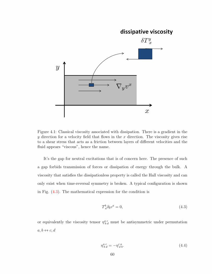
Figure 4.1: Classical viscosity associated with dissipation. There is a gradient in they direction for a velocity field that flows in the x direction. The viscosity gives riseto a shear stress that acts as a friction between layers of different velocities and thefluid appears “viscous”, hence the name.
It’s the gap for neutral excitations that is of concern here. The presence of such
a gap forbids transmission of forces or dissipation of energy through the bulk. A
viscosity that satisfies the dissipationless property is called the Hall viscosity and can
only exist when time-reversal symmetry is broken. A typical configuration is shown
in Fig. (4.3). The mathematical expression for the condition is
T ba∂bva = 0, (4.3)
or equivalently the viscosity tensor ηa cb d must be antisymmetric under permutation
a, b↔ c, d
ηa cb d = −ηc ad b. (4.4)
60

Figure 4.2: Spectrum of 10 electrons in 30 orbitals on the torus with V1 pseudopoten-tial interaction. The Laughlin ground state is set at the origin (zero momentum andzero energy). The magneto-roton mode merges into the multi-roton continuum inthe long wavelength limit. The roton-minimum defines the gap for a FQHE system.(Plot courtesy: F. D. M. Haldane).
The fact that there is no transmission of forces implies that a quantum Hall fluid
does not support a hydrostatic pressure. An external force acting upon the edge will
only modify the velocity of the edge currents and have no impact on the bulk, as
illustrated in Fig.(4.4). Since pressure is the trace of the stress tensor, this dictates
the traceless condition
T aa = 0. (4.5)
Note that a gapped quantum incompressible fluid is quite different than a classical
incompressible liquid. The incompressibility of a classical liquid is just a thought-
61

Figure 4.3: Hall viscosity for a velocity field that flows in the x direction with agradient in the y direction . The stress on the top and bottom surfaces is perpendicularto the flow velocity and therefore there is no dissipation of energy. The stress triesto deform the local fluid while preserving the area, i.e., it is traceless.
experiment where we send the sound-wave velocity to infinity. The consequence is that
the liquid supports a hydrostatic pressure that is instantaneously uniform throughout
the liquid. In contrast, a quantum Hall fluid doesn’t support sound waves due to the
presence of a gap for collective excitations.
These two constraints (dissipationlessness and tracelessness) significantly reduce
the number of free matrix elements in the viscosity tensor. In particular, in 2D we
have 3 independent elements that can be represented by a symmetric rank-2 tensor
62

Figure 4.4: Sketch of a quantum Hall droplet under a external force on the edge thattries to compress the system. The edge flow velocity increases and absorbs the forcewhile the interior feels no impact.
ηHab. This is shown as
ηe fb d = εaeεcfηHabcd, (4.6)
ηHabcd = ηHbacd = ηHabdc = −ηHcdab
= 12ε(εacη
Hbd + εadη
Hbc + εbcη
Had + εbdη
Hac
), (4.7)
where ε ≡ ε12 is the Pfaffian of the 2D Levi-Civita symbol. The tensor ηHab is odd
under time-reversal and will be called the 2D Hall viscosity tensor.
The 2D Hall viscosity tensor was first calculated for the IQHE by Avron, Seiler and
Zograf[3]. Later Read[36] generalized the calculation to include the FQHE assuming
63

rotational symmetry. There ηHab is proportional to the Euclidean metric
ηHab = ηHδab, (4.8)
with the scalar ηH interpreted as the density of “intrinsic orbital angular momentum”
ηH = 12~nes, (4.9)
where ne = ν/2πl2B is the electron density and s is the average orbital angular mo-
mentum. For the IQHE, the orbital angular momentum for the nth Landau level is
numerically equal to the topological spin sn = n + 12
defined in the previous chap-
ter, and this coincidence led to an identification in the literature between the scalar
Hall viscosity and the shift. However, the two quantities have completely different
origins. We elaborated on the topological nature of the shift (or the topological spin)
in Sec.(3.3) while the concept of “angular momentum” depends on the presence of
rotational symmetry. In a generic setting, these two quantities should have no rela-
tions. In the next section we will derive a generic formula for the 2D Hall viscosity
tensor, which is, perhaps not surprisingly, proportional to the natural metric specific
to each Landau level.
4.3 2D Hall viscosity tensor
Let’s revisit the definition of the stress tensor. In a variational approach, the stress
tensor is defined through the variation of an action under an infinitesimal diffeomor-
phism of the matter fields ϕ(x) 7→ ϕ(x′) = ϕ(x+ δu(x)),
δS =
∫d4x√
(−g)T µν∇µδuν , (4.10)
64

where ∇a is the covariant derivative associated with the metric gµν and√
(−g) is the
square root of the determinant of gµν . In field theory the stress tensor is also defined
as the variation against a change in the inverse metric
δS = −12
∫d4x√
(−g)Tµνδgµν . (4.11)
However, it is clear that the two definitions give two tensors of different index place-
ment. We argued in Sec.(4.1) that the stress tensor should be a (1,1) tensor, so
the first definition is fundamental. Then what is wrong with the second definition?
Actually it assumes there is a Lorentz symmetry so that
gµσTσν − T σµgσν = 0, (4.12)
i.e., the tensor Tµν ≡ gµσTσν is symmetric, which is implicit in the second definition.
Notice that the change in the inverse metric under the diffeomorphism is
δgµν = −(gµσ∇σδuν + gνσ∇σδu
µ), (4.13)
with which we can show that the two definition are equivalent when Eq.(4.12) is valid.
To explicitly calculate the stress tensor for a generic Hamiltonian, we will use the
fundamental definition in Eq.(4.10) for an action describing a 2DEG in U(1) gauge
fields A0 and Aa
S =
∫d2xdtL, (4.14)
L =i
2~ψ†∂0ψ −
i
2~(∂0ψ
†)ψ + eA0ψ†ψ −H, (4.15)
65

where the fermionic fields obey the algebra
{ψ(x), ψ(x′)} = {ψ†(x), ψ†(x′)} = 0, (4.16)
{ψ(x), ψ†(x′)} = iδ(2)(x− x′). (4.17)
We have assumed that the underlying manifold is the 2D Euclidean plane, i.e., gab =
δab and√g = 1. The Hamiltonian density H is just the generic form (2.30) written
in the field theoretic language. For example, for a system with Galilean invariance it
is just
H =1
2mab(Daψ)†Dbψ, (4.18)
Da = ~∂a − ieAa. (4.19)
Under an infinitesimal spatial diffeomorphism x′a = xa + δua the U(1)-covariant
derivatives transform as
D′a = (δba − ∂aδub)Db, (4.20)
and the variation of the action is
δS =
∫d2xdt T ab∂aδu
b, (4.21)
T ab =δH
δ(Daψ)†(Dbψ)† +
δHδ(Daψ)
Dbψ + Lδab . (4.22)
For the IQHE, which is essentially a single-particle problem, the stress tensor can be
written in terms of single-particle operators by tracing out the guiding-center part
Tr(eiq·R) = 2πδ2(q`B). (4.23)
66

The result is then (the Lδab term is identically zero and dropped)
T ab =1
2πl2Bτab, (4.24)
τab =1
2{va, pb}, va =
∂H(p)
∂pa= i(~eB)−1εab[pb, H], (4.25)
where H(p) is the single-particle Hamiltonian. The traceless part of the stress tensor
can also be obtained
τab = τab − 12τ ccδ
ab = −iεac[γbc, H(p)], (4.26)
where the γab operators are defined in Eq.(2.19).
Now we are ready to calculate the response of the stress tensor to a spatially-
uniform time-varying shear strain ∂aδub(t) ≡ λba(t). The perturbative Hamiltonian
is
δε(t) = −τab λba(t) = −τabλba(t), (4.27)
where we have used the fact that λaa(t) = 0 (shear strain). According to linear
response theory, the induced stress is determined by the retarded stress-stress corre-
lation function,
τab(t) =
∫dt′Ga c
b d(t− t′)λdc(t′), (4.28)
Ga cb d(t) =
∑n
νn~iΘ(t)〈Ψn|[τab(t), τ cd(0)]|Ψn〉, (4.29)
where Θ(t) is the step function (Θ(t) = 1 for t ≥ 0 and Θ(t) = 0 for t < 0), νn = 0 or
1 is the filling factor for the nth Landau level and Ψn are the eigenstates of H. We
67

then Fourier-transform it into frequency space,
Ga cb d(ω) =
∫dt ei(ω+iη)tGa c
b d(t), (4.30)
where η is an infinitesimal positive number. The Hall viscosity is the response to
the time derivative of the strain, which corresponds to the first order term in the
ω-expansion,
dGa cb d(ω)
dω
∣∣∣∣ω=0
=∑n,n′
~νn(En − En′)2
(〈n|τab|n′〉〈n′|τ cd|n〉 − 〈n|τ cd|n′〉〈n′|τab|n〉)
=∑n
~νnεaeεcf〈n|[γbe, γdf ]|n〉. (4.31)
where En are the Landau level energies and we simplified our notation by |Ψn〉 ≡ |n〉.
Comparing it to the definition of the viscosity (4.1), we arrive at the expression for
the rank-4 tensor
ηHabcd = − i~2πl2B
∑n
νn〈n|[γbc, γde]|n〉. (4.32)
Recall the commutator of the γab operators in Eq.(2.20), and we obtain the expression
for the 2D Hall viscosity tensor
ηHab =~
2πl2B
∑n
νn〈n|γab|n〉. (4.33)
We see that the contribution from each Landau level is proportional to its own natural
metric describing the shape of the orbits in that level. The natural metric has nothing
to do with the topological spin (although we used the natural metric to construct
coherent states that allowed us to define the topological spin). Only when rotational
68

symmetry is restored, all Landau levels have the same metric and
ηHab =~2
1
2πl2B
(∑n
νnsn
)δab, (4.34)
where sn = n+ 12
is numerically equal to the topological spin.
The generic formula has a property that it is diagonal with respect to the Landau
level index and doesn’t depend on inter-Landau-level mixing. In the next chapter
where we calculate electromagnetic responses, we will differentiate between universal
terms that are diagonal and non-universal terms that depend on inter-Landau-level
mixing.
4.4 Dipole on the edge
In the last section we showed that the generic Hall viscosity should not be identified
with the topological spin. However it does have a relation with a property on the
edge. Haldane[18] first pointed out that the Hall viscosity, a quantity defined in the
bulk, is related to the intrinsic dipole moment on the edge. This is a manifestation
of the bulk-edge correspondence.
To understand this relation, note that there is a discontinuity of the Hall viscosity
on the boundary. This discontinuity leaves a net stress force on the boundary, which,
for the boundary to remain static, must be balanced by a force from the electric field
gradient (that induces the velocity gradient) on an intrinsic electric dipole moment
dpa. Let dLa be an infinitesimal line segment on the boundary, then
T badLb = ηa cb d∇cv
ddLb = −dpb∇bEa. (4.35)
69
Using
va =εabEbB
, (4.36)
we have
dpa = B−1εabηHbcdLc. (4.37)
This correspondence allows a calculation of ηHbc from the edge dipole[34]. For the
IQHE, the dipole on the edge is related to the shape of the Gaussian tail and this is
consistent with our generic result Eq.(4.33) where ηHbc is proportional to the natural
metric that describes the shape of the Landau orbits. For the FQHE, apart from
the dipole of the Gaussian tail, there is another contribution coming from the dipole
of orbital occupation number. Fig.(4.4) gives the profile of occupation number for
Laughlin 1/3 state. Toward the edge the occupation number rises to a peak and
then drops steeply. This behavior is due to the squeezing property of the model
wavefunction mentioned in Sec.(1.2).
70

Figure 4.5: Occupation number n(k) for 15 electrons in Lauglin 1/3 state on a cylinderwith varying circumferences L from 12.5 to 22 with an increment of 0.5. The dashedline is the average 1/3.[34]
71

Chapter 5
Electromagnetic responses
In this chapter we will discuss the electromagnetic responses of particle- and current-
density without Galilean or rotational symmetry. We will add ingredients to the
Heisenberg algebra that will come in handy in our calculation. Particularly, a formal
expansion for the current-density operator in momentum space is provided. Then the
generic response functions will be derived and compared with previous results in the
literature. The identification due to Galilean invariance between the 2D Hall viscosity
and the q2 term in the Hall conductivity will be shown to break down in the generic
case and our approach uncovers hidden geometrical properties in the IQHE.
5.1 Heisenberg algebra
In the previous chapters we have made use of the Heisenberg algebra h2 of the momen-
tum operators whose commutator is a c-number. The universal enveloping algebra
U(h2) is spanned by the basis
{1, pa, {pa, pb}, {pa, pb, pc}, . . . } (5.1)
72

where {A,B, . . . , C} is the symmetrized product of n operators normalized so that
{λA, λA, . . . , λA} = n!(λA)n. The single-particle Hamiltonian is built on U(h2). The
Hamiltonian in this chapter will be in its most generic form
h = H(p) ≡∑n
1
n!Ha1,a2,...ann pa1pa2 . . . pan (5.2)
where the coefficients Ha1...ann are fully symmetric in all indices.
When deriving the Hall viscosity formula we used the derivative of the Hamiltonian
with the momentum components. Here we will define the derivative in a more formal
way using the unitary boost operator parametrized by a real c-number vector q
U(q) = U(−q)† = eiq·R, [qa, qb] = 0. (5.3)
Then
U(−q)pU(q) = p + ~q. (5.4)
and the derivatives ha1a2...an of h are defined by
h(q) ≡ U(−q)hU(q) =∞∑n=0
~n
n!ha1a2...anqa1qa2 . . . qan , (5.5)
where the tensor-valued operators ha1a2...an are fully symmetric in their indices. In
particular, the first derivative ha is the velocity operator va. Note also that
U(−q)U(−q′)pU(q′)U(q) = U(−(q + q′))pU(q + q′). (5.6)
From this
U(−q)ha1,...amU(q) =∞∑n=0
~n
n!ha1...amb1...bnqb1 . . . qbn . (5.7)
as in the differentiation of c-number functions, where (f ′)′ = f ′′.
73
Now let a ∈ U(h) be a vector-valued operator and λ be a c-number. Then define
the expansion
H(p + λa) = h+ λh1(a) +O(λ2). (5.8)
The quantity h1(a) can be expressed in two equivalent ways as the nested-commutator
expansions
h1(a) = aa1ha1 +
1
2![pa1 , aa2 ]h
a1a2 +1
3![pa1 , [pa2 , aa3 ]]h
a1a2a3 + . . . (5.9)
= ha1aa1 +1
2!ha1a2 [aa1 , pa2 ] +
1
3!ha1a2a3 [[aa1 , pa2 ], pa3 ] + . . . . (5.10)
This will be useful when we introduce perturbation to the gauge fields and thus to
the momentum operators.
The operator h is also a function of the scale factor B0, the constant magnetic
field, and more properly should be written as h(B0). The magnetization operator
m(p) is defined by
m ≡ − ∂h
∂B0
∣∣∣∣{Hn}
= −12B−10 h1(p)
= −12B−10 v · p = −1
2B−10 p · v = 1
2B−10
(h+ i`−2B εabR
ahRb). (5.11)
If the Hamiltonian is a quadratic operator, h = 12Hab
2 papb, then B0m = −h, i.e. the
shape of the Landau orbits is independent of the scaling of the magnetic field. This
is also true for a rotationally invariant Hamiltonian. Actually for any scalar operator
O ∈ U(h2), one can define the scale derivative
dO ≡ B0∂O
∂B0
= 12
(−i`−2B εabR
aORb −O), (5.12)
and by definition
dh = −B0m. (5.13)
74
Higher orders of derivatives can be recursively defined as
dn+1O ≡ B0∂(dnO)
∂B0
, d1O ≡ dO. (5.14)
Note that if Q ≡ q · R ∈ h, then
QORa − RaOQ = [Q,Ra](O + 2dO) (5.15)
where [Q,Ra] is a c-number,
For IQHE, the only formula we need for the guiding-center part is
Tr(eiq·R) = 2πδ2(q`B) (5.16)
where the trace is over the Hilbert space of the guiding-center, and δ2(x) is the 2D
Dirac delta-function.
5.2 Current density operator
In this section we will derive an expansion of the current-density operator to all orders
in q. Introduce an additional vector potential
Aa(x) =
∫d2q
(2π)2Aa(q)eiq·x, (5.17)
with
δB(x) = ∂1A2(x)− ∂2A1(x), (5.18)
and define the operator
Aa ≡∫
d2q
(2π)2Aa(q)eiq·RU(q). (5.19)
75

The problem of the charged particle moving in the 2D plane x in the presence of a
non-uniform magnetic flux density B0 + δB(x) is then described by the Hamiltonian
H = H(p− eA). (5.20)
The electric charge density operator is given by
J0(x) = e
∫d2q
(2π)2eiq(R−x)U(q), (5.21)
and the electric current-density operator is given by
Ja(x) = e
∫d2q
(2π)2eiq·(R−x)Ja(q). (5.22)
To find the expression for Ja(q), notice the continuity equation (gauge invariance)
requires
(i~)−1[J0(x), h] + ∂aJa(x) = 0, (5.23)
or in the q space
[h, U(q)] = ~qaJa(q). (5.24)
Then the functional form of the expansion of Ja(q) must be
~Ja(q) = −i[αa(q), h] + iεbaqb`2Bβ(q). (5.25)
where
iqaαa(q) = U(q)− 1 (5.26)
or
αa(q) = −i ∂∂qa
(∞∑n=1
1
n
(iq · R)n
n!
)=∞∑n=1
1
n
1
n!
n∑k=1
(iQ)k−1Ra(iQ)n−k. (5.27)
76

This must be satisfied at each order of an expansion in Aa(q) and to leading order
eaJa(q) = h1(eU(q)) +O(A), (5.28)
where e is a c-number unit vector. In this section we focus on the first term h1(eU(q)).
Using (5.9) the explicit form of Ja(q) can be written as
i~Ja = U(q)
([Ra, h] +
1
2![−iQ, [Ra, h]] +
1
3![−iQ, [−iQ, [Ra, h]]] + · · ·
), (5.29)
where Q = q · R as mentioned above. Expanding U(q) and the nested commutators
gives
i~Ja =∞∑m=0
(iQ)m
m!
∞∑n=0
(−1)n1
(n+ 1)!
n∑k=0
(−1)k(n
k
)(iQ)n−k[Ra, h](iQ)k. (5.30)
Recollect the terms in the form of
(iQ)l[Ra, h](iQ)k
and the corresponding coefficient Cl,k is (using l + k = m+ n)
Cl,k =l∑
m=0
1
m!(−1)l+k−m
1
(l + k −m+ 1)!(−1)k
(l + k −m
k
)
=1
k!l!
l∑m=0
(−1)m1
k +m+ 1
(l
m
)=
1
(k + l + 1)!. (5.31)
Now a significantly simplified form for Ja(q) can be written down
i~Ja =∞∑n=0
1
(n+ 1)!
n∑k=0
(iQ)n−k[Ra, h](iQ)k, (5.32)
77

which is further reduced into the desired form:
i~Ja =∞∑n=0
1
(n+ 1)!
((iQ)nRah− hRa(iQ)n − i
n−1∑k=0
(iQ)n−1−k(QhRa − RahQ)(iQ)k
)
=∞∑n=0
1
(n+ 1)!
(1
2{(iQ)n, Ra}h+
1
2[(iQ)n, Ra]h− 1
2h{Ra, (iQ)n}+
1
2h[(iQ)n, Ra]
−i[Q, Ra]n−1∑k=0
(iQ)n−1−k(h+ 2dh)(iQ)k
)
=∞∑n=0
1
(n+ 1)!
([1
2{(iQ)n, Ra}, h
]− i[Q, Ra]
n−1∑k=0
(iQ)n−1−k(2dh)(iQ)k
+i[Q, Ra]
(n
2(iQ)n−1h+
n
2h(iQ)n−1 −
n−1∑k=0
(iQ)n−1−kh(iQ)k
))
= [αa(q), h] + i[Q, Ra]β(q) (5.33)
where
αa(q) =∞∑n=0
1
2(n+ 1)!{(iQ)n, Ra}, (5.34)
β(q) = −∞∑n=0
2
(n+ 1)!
n−1∑k=0
(iQ)n−1−k(dh)(iQ)k +∞∑n=0
1
2(n+ 1)!
n−1∑k=0
[(iQ)n−1−k, [(iQ)k, h]].
(5.35)
The expansion for αa(q) agrees with the universal form (5.27), and the leading
term in β(q) is just −dh = B0m.
78

5.3 Response functions
We are ready to calculate the responses for a non-uniform magnetic field and a non-
zero electric field. The perturbed Hamiltonian is
H = h− e∫
d2q
(2π)2A0(q)U(q)eiq·R − e
∫d2q
(2π)2Aa(q)Ja(q)eiq·R
− e2∫
d2q
(2π)2Aa(−q)Γab(q)Ab(q)eiq·R +O(A3
a), (5.36)
where Γab(q) is a gauge counter-term that is important for ensuring gauge invariance.
It gives the O(A) dependence of the complete current-density operator. Its explicit
form is:
Γab(q) =1
~2∞∑n=0
1
(n+ 2)![
n︷ ︸︸ ︷iQ, · · · [iQ, [Ra, [h, Rb]]] · · · ]
+1
~2∞∑n=0
1
(n+ 2)![
n︷ ︸︸ ︷−iQ, · · · [−iQ, [Ra, [h, Rb]]] · · · ]
=1
~2∞∑k=0
2
(2k + 2)![
n︷ ︸︸ ︷iQ, · · · [iQ, [Ra, [h, Rb]]] · · · ]. (5.37)
The perturbed particle density and current density in the nth Landau level are
δJ0n(x) = − e
2π`2B
(∫d2q
(2π)2χ00n (q)U(q)eiq·x +
∫d2q
(2π)2χ0an (q)Aq(q)eiq·x
), (5.38)
δJan(x) = − e
2π`2B
(∫d2q
(2π)2χ0an (−q)A0(q)eiq·x +
∫d2q
(2π)2χabn (q)Ab(q)eiq·x
), (5.39)
where the correlation functions are density-density
χ00n (q) =
∑n′(6=n)
〈n|U(−q)|n′〉〈n′|Ua(q)|n〉+ 〈n|U(q)|n′〉〈n′|U(−q)|n〉En − En′
, (5.40)
79

density-current
χ0an (q) =
∑n′(6=n)
〈n|U(−q)|n′〉〈n′|Ja(q)|n〉+ 〈n|Ja(q)|n′〉〈n′|U(−q)|n〉En − En′
, (5.41)
current-current
χabn (q) =∑n′( 6=n)
〈n|Ja(−q)|n′〉〈n′|J b(q)|n〉+ 〈n|J b(q)|n′〉〈n′|Ja(−q)|n〉En − En′
, (5.42)
and current-current plus counter-term
χabn (q) = χabn (q) + 〈n|Γab(q)|n〉, (5.43)
and En and |n〉 are eigen-energies and eigenstates. Below we will simplify our notation
by defining
(A,B)n ≡∑n′ 6=n
〈n|A|n′〉〈n′|B|n〉+ 〈n|B|n′〉〈n′|A|n〉En − En′
, (5.44)
so
χ00n (q) = (U(−q), U(q))n, (5.45)
χ0an (q) = (U(−q), Ja(q))n, (5.46)
χabn (q) = (Ja(−q), J b(q))n. (5.47)
We will also denote the expectation value of some operator O in the nth Landau level
by 〈O〉n.
80

Using the expansions of U(q) and Ja(q), these correlation functions are readily
obtained:
χ00n (q) = −(Q,Q)n +O(|q|4), (5.48)
χ0an (q) = −1
~[Q, Ra]
(1− 1
6〈Q2〉n +
1
3(Q, {Q, dh})n −
1
2(Q2, dh)n
)+O(|q|5),
(5.49)
χabn (q) = − 1
~2[Q, Ra][Q, Rb]
(〈dh+ d2h〉n + (dh, dh)n
)+O(|q|4). (5.50)
If we define
χabE,n = − e2
2πl2B(Ra, Rb)n, (5.51)
σabn =1
6sng
abn −
[1
6(Ra, {Rb, dh})n + a↔ b
]+
1
4({Ra, Rb}, dh)n, (5.52)
sngabn =
1
2〈{Ra, Rb}〉n, (5.53)
χM,n =e2l2B2π~2
(〈dh+ d2h〉n + (dh, dh)n
), (5.54)
then
χ00n (q) = −2πl2B
e2qaqbχ
abE,n +O(|q|4), (5.55)
χ0an (q) = −1
~[Q, Ra]
(1− σabn qaqb
)+O(|q|5), (5.56)
χabn (q) = − 2π
e2l2B[Q, Ra][Q, Rb]χM,n +O(|q|4). (5.57)
Now using
[Q, Ra] = il2Bεbaqb, (5.58)
E(q) = iqA0(q), (5.59)
δB(q) = iεabqaAb(q), (5.60)
81

we are able to write down the generic responses (in the absence of rotational sym-
metry) of particle- and current- density against a non-vanishing electric field and a
non-uniform magnetic field:
δJan =1
2πl2B
(1 + σcdn ∂c∂d
)va − χM,nε
ab∂bδB, (5.61)
δJ0n =
1
2πl2B
(δB
B0
+ σabn ∂a∂b lnδB
B0
)− χabE,n∂aEb, (5.62)
where the magnetic length lB is defined with respect to B0 and va = εabEb/B0 is the
flow velocity field. Now the physical meaning of the previously defined quantities are
obvious: χabE (dropping the Landau level index) is the electric susceptibility tensor
that produces a polarization density P a = χabEEb, σab is the tensor in the q2 term of
the Hall conductivity and χM(B0) is the magnetic susceptibility at B0 that produces
an extra magnetic moment density δM = χMδB.
5.4 Discussion
We present here again the generic formula for σab, the q2 term of the Hall conductivity,
σabn =1
6sng
ab −[
1
6(Ra, {Rb, dh})n + a↔ b
]+
1
4({Ra, Rb}, dh)n. (5.63)
The first term is proportional to the inverse of the 2D Hall viscosity tensor ηHab. We
mentioned in the last chapter that terms being diagonal with respect to the Landau
level index are universal as they don’t depend on inter-Landau-level mixing. The
second and the third terms are inter-Landau-level mixing terms, with the second
term between states with opposite parity and the third term the same parity. They
depend on the details of the Hamiltonian and are non-universal. When there is
rotational symmetry, the third term vanishes because the eigenstates are invariant
with respect to rescaling of B0. When Galilean symmetry is present, the second term
82

can be explicitly calculated to be
−[1
6(Ra, {Rb, dh})n + a↔ b] =
4
3sng
ab, (5.64)
which combined with the first term gives
σabn =3
2sng
ab. (5.65)
This agrees with existing results in the literature[1, 38, 24, 5]. However a simple
identification of this tensor as the (inverse) 2D Hall viscosity tensor is not valid for a
realistic system and thus can not be relied on to measure the Hall viscosity.
The electric susceptibility tensor χabE measures the polarization energy at the pres-
ence of a electric field. In a quantum Hall fluid the electric field also induces a flow
velocity va = εabEb/B0 of the guiding centers. From the perspective of the guiding
centers the same energy can be interpreted as the kinetic energy of the guiding centers
and the tensor
mab = B20εacεbdχ
cdE (5.66)
acts as the effective mass of the guiding centers. Fig.(5.1) illustrates this idea. Note
that this effective mass has nothing to do with the effective mass in a Galilean invari-
ant Hamiltonian that is induced from the band structure.
The magnetic susceptibility χM has two terms. The first term is universal and we
can write it as
1
2πl2B〈2mB0
+∂m
∂B0
〉n. (5.67)
83

Figure 5.1: Sketch of the formation of a polarization P as the displacement of thecenter of the wave packet from the original guiding center under an electric field E.The guiding center will have a flow velocity determined by va = εabEb/B. There-fore the induced energy can be considered as either an polarization energy from theLandau-orbit point of view or a kinetic energy from the guiding-center point of view.
The ∂m/∂B0 part accounts for the change in the magnetization m in the nth Landau
level and vanishes for a Galilean system. The second term in χM is inter-Landau-
level mixing and accounts for the change of the Landau-orbit shape under scaling of
the magnetic field when rotational symmetry is absent. Fig.(5.4) summarizes these
different cases.
84

Figure 5.2: Sketch of the magnetization m under a change in the magnetic field. Thearea enclosed by the loops indicate the magnitude of m and the shape is that of theLandau orbits. For a Galilean invariant system, m doesn’t change. For a rotationallyinvariant system, the change in m originates within a single Landau level and theshape of the Landau orbits doesn’t change. In the generic case, the change in m hascontributions both from within the Landau level and from inter-Landau-level mixingthat also changes the shape of the Landau orbits.
85

Chapter 6
Conclusion
We presented a generic theory for the IQHE in the absence of Galilean or rotational
symmetry. We introduced the algebra of Landau orbits and guiding centers, and used
the natural metric of each Landau level to construct guiding-center coherent states.
Then we achieved the following three things:
• By numerically solving the eigen problem for a quartic Hamiltonian and in-
vestigating the root distribution of the polynomial solutions, we defined the
topological spin as the number of central zeros that are enclosed by a fattened
version of the semiclassical orbit.
• We calculated the generic formula for the 2D Hall viscosity tensor and found
that the contribution from each Landau level is proportional to its natural
metric. We also pointed out the identification of the scalar Hall viscosity with
the topological spin is only a coincidence at the presence of rotational symmetry.
• We obtained generic electromagnetic responses and clarified the structure of
the correlation functions. Particularly the q2 term of the Hall conductivity was
shown to differ from the (inverse) 2D Hall viscosity in the generic case as it
contains inter-Landau-mixing terms that are non-universal.
86

These results have clearly shown that the generic approach is able to:
• differentiate between topological and non-topological quantities;
• reveal richer geometrical properties previously hidden by applying special sym-
metries.
A possible direction to carry this research further would be a close study on the
“gravitational anomaly” term that appears in the effective theory for the QHE[8, 1,
14, 10, 16]. Previous work has treated the metric as that of the underlying manifold.
Although the mathematics is well developed in the field theory, that approach doesn’t
explain much about the physical nature of the term. We believe a truly physical
interpretation should be that the metric is a dynamic quantity intrinsic to the system
and something that is able to induce a variation in the metric would be either acoustic
waves of the underlying crystal lattice or the interactive dynamics of the 2DEG itself.
Also Galilean symmetry is not essential to the presence of the term and we would
like to see a generic derivation.
It would certainly be wonderful if we could extend this generic approach to the
FQHE. In fact, all the concepts used in this thesis have their counterparts in the
FQHE and some are indeed mentioned in the discussion. For example, the guiding-
center counterpart of the polarization effect in the electromagnetic responses would be
due to a shift of the position of the electron away from the center of flux attachment
or correlation hole. It is also likely that new concepts, especially geometrical ones,
that have no counterparts in the IQHE can emerge in the FQHE when we pursue a
generic approach.
87

Bibliography
[1] Alexander G. Abanov and Andrey Gromov. Electromagnetic and gravitationalresponses of two-dimensional noninteracting electrons in a background magneticfield. Phys. Rev. B, 90:014435, Jul 2014.
[2] Daniel Arovas, J. R. Schrieffer, and Frank Wilczek. Fractional statistics and thequantum hall effect. Phys. Rev. Lett., 53:722–723, Aug 1984.
[3] J. E. Avron, R. Seiler, and P. G. Zograf. Viscosity of quantum hall fluids. Phys.Rev. Lett., 75:697–700, Jul 1995.
[4] B. Andrei Bernevig and F. D. M. Haldane. Model fractional quantum hall statesand jack polynomials. Phys. Rev. Lett., 100:246802, Jun 2008.
[5] R. R. Biswas. Semiclassical theory of viscosity in quantum hall states.arXiv:1311.7149, Dec 2013.
[6] Parsa Bonderson, Victor Gurarie, and Chetan Nayak. Plasma analogy and non-abelian statistics for ising-type quantum hall states. Phys. Rev. B, 83:075303,Feb 2011.
[7] Barry Bradlyn and N. Read. Low-energy effective theory in the bulk for transportin a topological phase. Phys. Rev. B, 91:125303, Mar 2015.
[8] Barry Bradlyn and N. Read. Topological central charge from berry curvature:Gravitational anomalies in trial wave functions for topological phases. Phys. Rev.B, 91:165306, Apr 2015.
[9] J. M. Caillol, D. Levesque, J. J. Weis, and J. P. Hansen. A monte carlo studyof the classical two-dimensional one-component plasma. Journal of StatisticalPhysics, 28:325–349, June 1982.
[10] T. Can, M. Laskin, and P. Wiegmann. Fractional quantum hall effect in a curvedspace: Gravitational anomaly and electromagnetic response. Phys. Rev. Lett.,113:046803, Jul 2014.
[11] Gil Young Cho, Yizhi You, and Eduardo Fradkin. Geometry of fractional quan-tum hall fluids. Phys. Rev. B, 90:115139, Sep 2014.
88

[12] S. M. Girvin. The quantum hall effect: Novel excitations and broken symmetries.arXiv:cond-mat/9907002, July 1999.
[13] S. M. Girvin, A. H. MacDonald, and P. M. Platzman. Magneto-roton theoryof collective excitations in the fractional quantum hall effect. Phys. Rev. B,33:2481–2494, Feb 1986.
[14] Andrey Gromov and Alexander G. Abanov. Density-curvature response andgravitational anomaly. Phys. Rev. Lett., 113:266802, Dec 2014.
[15] Andrey Gromov and Alexander G. Abanov. Thermal hall effect and geometrywith torsion. Phys. Rev. Lett., 114:016802, Jan 2015.
[16] Andrey Gromov, Gil Young Cho, Yizhi You, Alexander G. Abanov, and EduardoFradkin. Framing anomaly in the effective theory of the fractional quantum halleffect. Phys. Rev. Lett., 114:016805, Jan 2015.
[17] F. D. M. Haldane. Fractional quantization of the hall effect: A hierarchy ofincompressible quantum fluid states. Phys. Rev. Lett., 51:605–608, Aug 1983.
[18] F. D. M. Haldane. Hall viscosity and intrinsic metric of incompressible fractionalhall fluids. arXiv:0906.1854, June 2009.
[19] F. D. M. Haldane. Geometrical description of the fractional quantum hall effect.Phys. Rev. Lett., 107:116801, Sep 2011.
[20] F. D. M. Haldane and E. H. Rezayi. Periodic laughlin-jastrow wave functionsfor the fractional quantized hall effect. Phys. Rev. B, 31:2529–2531, Feb 1985.
[21] F. D. M. Haldane and Y. Shen. Geometry of landau orbits in the absence ofrotational symmetry. arXiv:1512.04502v2, May 2016.
[22] B. I. Halperin. Statistics of quasiparticles and the hierarchy of fractional quan-tized hall states. Phys. Rev. Lett., 52:1583–1586, Apr 1984.
[23] M. Z. Hasan and C. L. Kane. Colloquium. Rev. Mod. Phys., 82:3045–3067, Nov2010.
[24] Carlos Hoyos and Dam Thanh Son. Hall viscosity and electromagnetic response.Phys. Rev. Lett., 108:066805, Feb 2012.
[25] J. K. Jain. Composite-fermion approach for the fractional quantum hall effect.Phys. Rev. Lett., 63:199–202, Jul 1989.
[26] K. v. Klitzing, G. Dorda, and M. Pepper. New method for high-accuracy deter-mination of the fine-structure constant based on quantized hall resistance. Phys.Rev. Lett., 45:494–497, Aug 1980.
[27] Ilpo Laine. Nevanlinna Theory and Complex Differential Equations. Walter deGruyter, 1993.
89

[28] R. B. Laughlin. Quantized hall conductivity in two dimensions. Phys. Rev. B,23:5632–5633, May 1981.
[29] R. B. Laughlin. Anomalous quantum hall effect: An incompressible quantumfluid with fractionally charged excitations. Phys. Rev. Lett., 50:1395–1398, May1983.
[30] Hui Li and F. D. M. Haldane. Entanglement spectrum as a generalization of en-tanglement entropy: Identification of topological order in non-abelian fractionalquantum hall effect states. Phys. Rev. Lett., 101:010504, Jul 2008.
[31] Gregory Moore and Nicholas Read. Nonabelions in the fractional quantum halleffect. Nuclear Physics B, 360(23):362 – 396, 1991.
[32] Maho Nakata. The mpack (mblas/mlapack): a multiple precision arithmetic ver-sion of blas and lapack, version 0.8.0, 2012, see http://mplapack.sourceforget.net.
[33] Chetan Nayak, Steven H. Simon, Ady Stern, Michael Freedman, and SankarDas Sarma. Non-abelian anyons and topological quantum computation. Rev.Mod. Phys., 80:1083–1159, Sep 2008.
[34] YeJe Park and F. D. M. Haldane. Guiding-center hall viscosity and intrin-sic dipole moment along edges of incompressible fractional quantum hall fluids.Phys. Rev. B, 90:045123, Jul 2014.
[35] Anthony Ralston and Philip Rabinowitz. A first course in numerical analysis.DOVER PUBLICATIONS, INC., 2001.
[36] N. Read. Non-abelian adiabatic statistics and hall viscosity in quantum hallstates and px + ipy paired superfluids. Phys. Rev. B, 79:045308, Jan 2009.
[37] N. Read and E. Rezayi. Beyond paired quantum hall states: Parafermions andincompressible states in the first excited landau level. Phys. Rev. B, 59:8084–8092, Mar 1999.
[38] D. T. Son. Newton-cartan geometry and the quantum hall effect.arXiv:1306.0638, June 2013.
[39] D. J. Thouless, M. Kohmoto, M. P. Nightingale, and M. den Nijs. Quantized hallconductance in a two-dimensional periodic potential. Phys. Rev. Lett., 49:405–408, Aug 1982.
[40] D. C. Tsui, H. L. Stormer, and A. C. Gossard. Two-dimensional magnetotrans-port in the extreme quantum limit. Phys. Rev. Lett., 48:1559–1562, May 1982.
[41] Klaus von Klitzing. The quantized hall effect. Rev. Mod. Phys., 58:519–531, Jul1986.
[42] X. G. Wen. Theory of the edge states in fractional quantum hall effects. Int. J.Mod. Phys. B, 06:1711, 1992.
90

[43] X. G. Wen and A. Zee. Shift and spin vector: New topological quantum numbersfor the hall fluids. Phys. Rev. Lett., 69:953–956, Aug 1992.
[44] R. Willett, J. P. Eisenstein, H. L. Stormer, D. C. Tsui, A. C. Gossard, and J. H.English. Observation of an even-denominator quantum number in the fractionalquantum hall effect. Phys. Rev. Lett., 59:1776–1779, Oct 1987.
[45] Bo Yang, Zi-Xiang Hu, Z. Papic, and F. D. M. Haldane. Model wave functionsfor the collective modes and the magnetoroton theory of the fractional quantumhall effect. Phys. Rev. Lett., 108:256807, Jun 2012.
[46] Bo Yang, Z. Papic, E. H. Rezayi, R. N. Bhatt, and F. D. M. Haldane. Bandmass anisotropy and the intrinsic metric of fractional quantum hall systems.Phys. Rev. B, 85:165318, Apr 2012.
[47] Michael P. Zaletel and Roger S. K. Mong. Exact matrix product states forquantum hall wave functions. Phys. Rev. B, 86:245305, Dec 2012.
91
![Anisotropy in the Integer Quantum Hall E ect · 2018-04-24 · ux quantum [19]. The fractional quantum Hall E ect (FQHE) has many unusual properties not found in the integer quantum](https://img.pdfslide.net/doc/110x75/5f528e89fe3e2a4cf715bf97/anisotropy-in-the-integer-quantum-hall-e-ect-2018-04-24-ux-quantum-19-the-fractional.jpg)


![Noncommutative Quantum Field Theoryhep.itp.tuwien.ac.at/~miw/documents/hoffnung-3.pdf · physics to the integer quantum Hall effect [3]. Gauge models on the two-dimensional non-commutative](https://img.pdfslide.net/doc/110x75/5fbfe5b458086349120abf90/noncommutative-quantum-field-miwdocumentshoffnung-3pdf-physics-to-the-integer.jpg)


![Nanoscopic Quantum Rings: ANewPerspective · the gauge-invariance interpretation of the integer quantum Hall effect and the current carrying edge states [5]. The phenomenon is resticted](https://img.pdfslide.net/doc/110x75/5e867ab59dd31030a1203a93/nanoscopic-quantum-rings-the-gauge-invariance-interpretation-of-the-integer-quantum.jpg)