European Journal of Operational Research 211 (2011) 612–622

Contents lists available at ScienceDirect

European Journal of Operational Research

journal homepage: www.elsevier .com/locate /e jor

Innovative Applications of O.R.

A genetic algorithm for the unrelated parallel machine scheduling problemwith sequence dependent setup times

Eva Vallada ⇑, Rubén RuizGrupo de Sistemas de Optimización Aplicada, Instituto Tecnológico de Informática, Universidad Politécnica de Valencia, Edificio 7A, Camino de Vera S/N, 46021 Valencia, Spain

a r t i c l e i n f o a b s t r a c t

Article history:Received 25 June 2009Accepted 4 January 2011Available online 9 January 2011

Keywords:Parallel machineSchedulingMakespanSetup times

0377-2217/$ - see front matter � 2011 Elsevier B.V. Adoi:10.1016/j.ejor.2011.01.011

⇑ Corresponding author. Tel.: +34 96 387 70 07x74E-mail addresses: evallada@eio.upv.es (E. Vallada),

In this work a genetic algorithm is presented for the unrelated parallel machine scheduling problem inwhich machine and job sequence dependent setup times are considered. The proposed genetic algorithmincludes a fast local search and a local search enhanced crossover operator. Two versions of the algorithmare obtained after extensive calibrations using the Design of Experiments (DOE) approach. We review,evaluate and compare the proposed algorithm against the best methods known from the literature.We also develop a benchmark of small and large instances to carry out the computational experiments.After an exhaustive computational and statistical analysis we can conclude that the proposed methodshows an excellent performance overcoming the rest of the evaluated methods in a comprehensivebenchmark set of instances.

� 2011 Elsevier B.V. All rights reserved.

1. Introduction

In the unrelated parallel machine scheduling problem, there is aset N = {1, . . . ,n} of n jobs that have to be processed on exactly onemachine out of a set M = {1, . . . ,m} of m parallel machines. There-fore, each job is made up of one single task that requires a givenprocessing time. Machines are considered unrelated when the pro-cessing times of the jobs depend on the machine to which they areassigned to. This is the most realistic case which is also a general-isation of the uniform and identical machines cases. Moreover, theconsideration of setup times between jobs is very common in theindustry. The setup times considered in this paper are both se-quence and machine dependent, that is, setup time on machine ibetween jobs j and k is different than setup time on the same ma-chine between jobs k and j. In addition, setup time between jobs jand k on machine i is different than setup time between jobs j andk on machine i0.

The most studied optimisation criterion is the minimisation ofthe maximum completion time of the schedule, a criteria that isknown as makespan or Cmax. Summing up, in this paper we dealwith the unrelated parallel machine scheduling problem with se-quence dependent setup times denoted as R/Sijk/Cmax (Pinedo,2008). We propose and evaluate a genetic algorithm that includesa fast local search and a local search enhanced crossover operatoramong other innovative features that, as we will see, result in astate-of-the-art performance for this problem.

ll rights reserved.

911; fax: +34 96 387 74 99.rruiz@eio.upv.es (R. Ruiz).

The remainder of this paper is organised as follows: in Section 2we review the literature on this problem. In Section 3 a Mixed Inte-ger Programing (MIP) model formulation is presented. In Section 4we describe in detail the proposed genetic algorithm and prelimin-ary computational results. In Section 5, a Design of Experimentsapproach is applied in order to calibrate the genetic algorithm. Re-sults of a comprehensive computational and statistical evaluationare reported in Section 6. Finally, conclusions are given inSection 7.

2. Literature review

Parallel machine scheduling problems have been widely studiedin the past decades. However, the case when the parallel machinesare unrelated has been much less studied. Additionally, the consid-eration of sequence dependent setup times between jobs has notbeen considered until recently. In Allahverdi et al. (2008) a recentreview of scheduling problems with setup times is presented,including the parallel machine case. In this section we focus ourattention on the available algorithms for the parallel machinescheduling problems considering setup times.

In the literature, we can find several heuristic and metaheuristicalgorithms for the mentioned problem. However, most of them arefocused on the identical parallel machine case. In Guinet (1993), aheuristic is proposed for the identical parallel machines case withsequence dependent setup times and the objective to minimise themakespan. A tabu search algorithm is given in Franca et al. (1996)with the objective to minimise the total completion time. A threephase heuristic is proposed by Lee and Pinedo (1997) for the same

E. Vallada, R. Ruiz / European Journal of Operational Research 211 (2011) 612–622 613

problem with sequence dependent setup times (independent ofthe machine) and the objective to minimise the sum of weightedtardiness of the jobs. In Kurz and Askin (2001), the authors pro-posed several heuristics and a genetic algorithm to minimisemakespan. Other heuristics for the same problem are those pro-posed by Gendreau et al. (2001) and Hurink and Knust (2001). Inboth cases the objective is to minimise the makespan and in thelatter case precedence constraints are also considered. In Eomet al. (2002) and Dunstall and Wirth (2005) heuristics are proposedfor the family setup times case. In Tahar et al. (2006) a linear pro-gramming approach is proposed where job splitting is also consid-ered. Anghinolfi and Paolucci (2007) and Pfund et al. (2008)present heuristic and metaheuristic methods for the same prob-lem, respectively.

The unrelated parallel machines case with sequence depen-dent setup times has been less studied and only a few paperscan be found in the literature. A tabu search algorithm is givenin Logendran et al. (2007) for the weighted tardiness objective.Another heuristic for the unrelated parallel machine case withthe objective to minimise weighted mean completion time isthat proposed by Weng et al. (2001). Kim et al. (2002) proposeda simulated annealing method with the objective to minimisethe total tardiness. In Kim et al. (2003) and Kim and Shin(2003) a heuristic and tabu search algorithm were proposed withthe objective to minimise the total weighted tardiness and themaximum lateness, respectively. The same problem is also stud-ied in Chen (2005), Chen (2006) and Chen and Wu (2006) whereresource constraints are also considered, with the objective tominimise makespan, maximum tardiness and total tardiness,respectively. In Rabadi et al. (2006) a heuristic for the unrelatedmachine case with the objective to minimise makespan is alsopresented. Rocha de Paula et al. (2007) proposed a method basedon the VNS strategy for both cases, identical and unrelated par-allel machines for the makespan objective. In Low (2005) andArmentano and Felizardo (2007) the authors proposed a simu-lated annealing method and a GRASP algorithm, with the objec-tive to minimise the total flowtime and the total tardiness,respectively.

Regarding the exact methods, there are some papers availablein the literature for the parallel machine problem. However, mostof them are able to solve instances with a few number of jobsand machines (more details in Allahverdi et al. (2008)).

In this paper, we deal with the unrelated parallel machinescheduling problem in which machine and job sequence depen-dent setup times are considered, i.e., the setup times depend onboth, the job sequence and the assigned machine. We evaluateand compare some of the above methods available in the literature.We also propose a genetic algorithm that shows excellent perfor-mance for a large benchmark of instances.

3. MIP mathematical model

In this section, we provide a Mixed Integer Programming (MIP)mathematical model for the unrelated parallel machine schedulingproblem with sequence dependent setup times. Note that thismodel is an adapted version of that proposed by Guinet (1993).We first need some additional notation in order to simplify theexposition of the model.

� pij: processing time of job j, j 2 N at machine i, i 2M.� Sijk: machine based sequence dependent setup time on machine

i, i 2M, when processing job k, k 2 N, after having processed jobj, j 2 N.

The model involves the following decision variables:

Xijk ¼1; if job j precedes job k on machine i

0; otherwise

�

Cij ¼ Completion time of job j at machine i

Cmax ¼Maximum completion time

The objective function is:

min Cmax; ð1Þ

And the constraints are:Xi2M

Xj2 0f g[ Nf g

j – k

Xijk ¼ 1; 8k 2 N; ð2Þ

Xi2M

Xk2N

j – k

Xijk 6 1; 8j 2 N; ð3Þ

Xk2N

Xi0k 6 1; 8i 2 M; ð4Þ

Xh2 0f g[ Nf g

h–k;h–j

Xihj P Xijk; 8j; k 2 N; j – k; 8i 2 M; ð5Þ

Cik þ Vð1� XijkÞP Cij þ Sijk þ pik; 8j 2 0f g [ Nf g; 8k

2 N; j – k; 8i 2 M; ð6Þ

Ci0 ¼ 0; 8i 2 M; ð7Þ

Cij P 0; 8j 2 N; 8i 2 M; ð8Þ

Cmax P Cij; 8j 2 N; 8i 2 M; ð9Þ

Xijk 2 0;1f g; 8j 2 0f g [ Nf g; 8k 2 N; j – k; 8i 2 M: ð10Þ

The objective is to minimise the maximum completion time ormakespan. Constraint set (2) ensures that every job is assigned toexactly one machine and has exactly one predecessor. Notice theusage of dummy jobs 0 as Xi0k, i 2M, k 2 N. With constraint set(3) we set the maximum number of successors of every job toone. Set (4) limits the number of successors of the dummy jobs toa maximum of one on each machine. With Set (5) we ensure thatjobs are properly linked in machine: if a given job j is processedon a given machine i, a predecessor h must exist on the same ma-chine. Constraint set (6) is to control the completion times of thejobs at the machines. Basically, if a job k is assigned to machine iafter job j (i.e., Xijk = 1), its completion time Cik must be greater thanthe completion time of j, Cij, plus the setup time between j and k andthe processing time of k. If Xijk = 0, then the big constant V rendersthe constraint redundant. Sets (7) and (8) define completion timesas 0 for dummy jobs and non-negative for regular jobs, respectively.Set (9) defines the maximum completion time. Finally, set (10) de-fines the binary variables. Therefore, in total, the model containsn2m binary variables, (n + 1)m + 1 continuous variables and2n2m + nm + 2n + 2m constraints. This MIP model will be used laterin the computational experiments.

4. Proposed genetic algorithm

Genetic algorithms (GAs) are bio-inspired optimisation meth-ods (Holland, 1975) that are widely used to solve scheduling prob-lems (Goldberg, 1989). Generally, the input of the GA is a set ofsolutions called population of individuals that will be evaluated.Once the evaluation of individuals is carried out, parents are se-lected and a crossover mechanism is applied to obtain a new gen-eration of individuals (offspring). Moreover, a mutation scheme is

614 E. Vallada, R. Ruiz / European Journal of Operational Research 211 (2011) 612–622

also applied in order to introduce diversification into the popula-tion. The main features of the proposed genetic algorithm are theapplication of a fast local search procedure and a local search en-hanced crossover operator. In the following subsections we reporta detailed description about the developed GA.

4.1. Representation of solutions, initialisation of the population andselection operator

The most commonly used solution representation for the paral-lel machine scheduling problem is an array of jobs for each ma-chine that represents the processing order of the jobs assigned tothat machine. This representation is complete in the sense thatall feasible solutions of the MIP model presented in Section 3 canbe represented (recall that Cmax is a regular criterion and thereforeno machine should be left idle when capable of being occupied by ajob). The GA is formed by a population of Psize individuals, whereeach individual consists of m arrays of jobs (one per machine).

It is also common to randomly generate the initial population ina genetic algorithm. However, a recent trend consists in includingin the population some good individuals provided by some effec-tive heuristics. One of the best heuristics for the parallel machinescheduling problem is the Multiple Insertion (MI) heuristic pro-posed by Kurz and Askin (2001). The MI heuristic starts by orderingthe jobs according to a matrix with the processing and setup times.After the initial solution, each job is inserted in every position ofevery machine and places the job in the position that results inthe lowest makespan. One individual of the population is obtainedby means of the MI heuristic and the remaining ones are randomlygenerated. However, in order to obtain a good initial population,

2

1

Fig. 1. Example of the local search enh

the MI heuristic is applied to the random individuals, that is, foreach random individual each job is inserted in every position ofevery machine and finally the job is placed in the position that re-sults in the best makespan.

Regarding the selection mechanism, in the classical geneticalgorithms, tournament and ranking-like selection operators arecommon. Such operators either require fitness and mapping calcu-lations or the population to be continuously sorted. In this work, amuch simpler and faster selection scheme, called n-tournament, isused (Ruiz and Allahverdi, 2007). In this case, according to aparameter called ‘‘pressure’’, a given percentage of the populationis randomly selected. The individual with the lowest makespan va-lue among the randomly selected percentage of individuals winsthe tournament and is finally selected. This results in a very fastselection operator, since for each individual the Cmax value can bedirectly used as a fitness value.

4.2. Local search enhanced crossover and mutation operators

Once the selection is carried out and the parents have been se-lected, the crossover operator is applied according to a probabilityPc. There are several crossover operators proposed in the literaturefor scheduling problems. In general, the goal of the crossover oper-ator is to generate two good individuals, called offspring, from thetwo selected progenitors. One of the most used crossover operatorsis the One Point Order Crossover adapted to the parallel machinecase. Therefore, for each machine one point p is randomly selectedfrom parent 1 and jobs from the first position to the p position arecopied to the first offspring. Jobs from the point p + 1 position tothe end are copied to the second offspring. In Fig. 1, an example

anced crossover operator (LSEC).

Fig. 2. Example with 7 jobs and 2 machines for the IMI local search.

E. Vallada, R. Ruiz / European Journal of Operational Research 211 (2011) 612–622 615

for 12 jobs and two machines is given (setup times between jobsare not shown for clarity). Two parents are shown and for each ma-chine a point p is selected (Fig. 1(a)). Specifically, point p1 (machine1) is set to 3 and point p2 (machine 2) is set to 4. Therefore, the firstoffspring is formed with the jobs of parent 1 from position 1 to 3 inmachine 1 and jobs from position 1 to 4 in machine 2. The secondoffspring will contain jobs of parent 1 from position 4 to the lastone in machine 1 and from position 5 to the last one in machine2 (Fig. 1(b)). Then, jobs from the parent 2 which are not alreadyin the offspring are inserted in the same order. At this point, it iseasy to introduce a limited local search procedure in the crossoveroperator. When missing jobs are inserted from the parent 2, theyare inserted in every position of the offspring at the same machineand finally the job is placed in the position that results in the min-imum completion time for that machine. In this way we obtain acrossover operator with a limited local search. In Fig. 1(b), jobsfrom parent 2 which are not already in the offspring will be in-serted, that is, jobs 7, 3, 2, 1 of machine 1 from parent 1 are alreadyinserted in offspring 1, so they are not considered. Job 5 will be in-serted in every position of machine 1 and finally will be placed inthe best position (lowest completion time of the machine). In ma-chine 2, jobs 10, 9, 12 and 11 will be inserted in every position ofthe machine 2 and will be placed in the best position. In a similarway, in offspring 2 jobs 7, 3, 2 and 1 will be inserted in every posi-tion of machine 1 and jobs 4, 6 and 8 will be inserted in every posi-tion of machine 2. In Fig. 1(c) we can see the offspring obtainedafter the application of the local search enhanced crossover opera-tor (remember that setup times are not represented). In Section 6,results after testing this local search enhanced crossover operator(LSEC) will be given.

Once we obtain the offspring, a mutation operator can be ap-plied according to a probability (Pm). After short experiments test-ing different mutation operators, the best performance wasobtained by the most usual in scheduling problems, that is, theshift mutation. A machine is randomly selected and then a job isalso randomly selected and re-inserted to a different position ran-domly chosen in the same machine.

4.3. Local search and generational scheme

Local search procedures are widely used in genetic algorithmsas well as in other metaheuristic methods to improve solutions.For the parallel machine scheduling problem with the objectiveto minimise the makespan, it is possible to apply a really fast localsearch procedure based on the insertion neighborhood, the mostused in scheduling problems. We test the inter-machine insertionneighborhood (IMI), which consists of, for all machines, insertionof all the jobs in every position of all the machines. In order to re-duce the computational effort needed by the local search, it is pos-sible to introduce a simple and very efficient speed up procedure:when a job is inserted, it is not necessary to evaluate the completesequence for obtaining the new completion time value of the ma-chine. Let us give an example, we have 7 jobs and 2 machines(Fig. 2), grey blocks represent the setup times between the jobs.Remember that these setup times are both machine and job se-quence dependent. Moreover, these setup times differ betweenmachines 2 and 1. The makespan value for the current shown solu-tion is 21 and a step of IMI local search is applied. For example, wehave that job 1 is going to be inserted on the second position ofmachine 2. To obtain the new completion time of the machines,we only have to remove the processing time of job 1 and the setuptime between job 1 and 3 on machine 1. Then, if we want to insertjob 1 on machine 2, we have to remove the setup time betweenjobs 2 and 4. Finally, we have to add the setup time between job2 and job 1 on machine 2, the processing time of job 1 on machine2, that could be different than the processing time of job 1 on ma-

chine 1, and the setup time between jobs 1 and 4 on machine 2. Sowe can obtain the new completion time of the machines (Fig. 2(b)),with only 3 subtractions and 3 additions and therefore, we can ob-tain the new makespan value (20) which is better than the previ-ous one. In general, for each insertion, the number ofsubtractions and additions will be four and four, respectively, ifthe job is not inserted in the first or last position. For insertionsin the first or last position, the number of subtractions and addi-tions will be three and three, respectively (there is not setup timeat the beginning or the end of the machine sequence).

In total, the proposed local search will contain the followingnumber of steps (inter-machine insertions):Xi2M

Xl2Ml–i

niðnl þ 1Þ;

where ni and nl are the number of jobs assigned to machine i and l,respectively, that is, each job on machine i can be inserted in nl + 1positions on machine l.

During the local search procedure, we have to decide whichmovements are accepted applying an acceptance criterion. In ouralgorithm, local search is based on the previous IMI neighborhood,so two machines are involved in the local search procedure. That is,the neighborhood is examined in the following way: for all the ma-chines, all the jobs assigned to this machine are inserted in all posi-tions of all other machines. However, the examination of theneighborhood is carried out between pairs of machines, that is,jobs assigned to machine 1 are inserted in all positions of machine2 and the acceptance criterion is applied. Then, jobs from machine1 are inserted in all positions of machine 3 and so on. For every pairof machines, the following acceptance criterion based on the newcompletion times of the machines after an insertion is analyzed:

� Completion time of both machines is reduced: this is the idealsituation since if the movement is applied both machinesreduce the completion time. Obviously, the movement isaccepted in this case.� Completion time of one machine is reduced and completion

time of the other machine is increased: in this case we haveto decide the acceptance of the movement. If the amount oftime reduced on one machine is greater than the amount oftime increased on the other machine and the makespan valueis not increased, then the movement is accepted. Specifically:– Ci;C

0i: completion time of machine i before and after the

insertion movement, respectively, i 2M.– Cl;C

0l: completion time of machine l before and after the

insertion movement, respectively, l 2M, l – i.

616 E. Vallada, R. Ruiz / European Journal of Operational Research 211 (2011) 612–622

– Cmax;C0max: makespan of the sequence before and after the

insertion movement, respectively.

Therefore, in this case the movement will be accepted when:

C0i < Ci; i 2 M; ð11Þ

and

C0l > Cl; l 2 M; ð12Þ

and

Ci � C 0i > C 0l � Cl; i; l 2 M; i – l; ð13Þ

and

C0max 6 Cmax; ð14Þ

With expression (11), the new completion time of machine iis reduced. Expression (12) shows that new completion timeof machine l is increased. Expression (13) compares theamount reduced vs. the amount increased and finally, expres-sion (14) tests the new makespan value.

Table 1Variants of the genetic algorithm proposed.

Version Local search enhanced crossover Local search

GAStd1 No NoGAStd2 Yes NoGAStd3 No YesGAStd4 Yes Yes

Table 2Standard parameter values for the four variants of thegenetic algorithm.

Parameter Value

Population size (Psize) 50Selection pressure (Pressure) 30Probability of crossover (Pc) 0.5Probability of mutation (Pm) 0.2Probability of local search (Pls) 0.4

� Completion time of both machines is increased: in this case themovement is not accepted.

Moreover, the IMI local search is applied until local optima, thatis, if after a step of the local search one or more movements are ac-cepted, which means an improvement, the IMI local search is ap-plied again from the beginning. As we can see, applying IMI untillocal optima results in a very intensive and fine tuned local search.This is only possible with the speed-ups and accelerations pro-posed. The local search procedure is applied according to a proba-bility (Pls) to the best individual of the initial population and to theoffspring. The way to accept movements in the local search is animportant feature of the algorithm. We will see in Section 6 the ef-fect of the local search, that improves the results significantly.Moreover, different ways to accept movements were tested obtain-ing much worse results, so the idea to accept movements analyzingthe machines by pairs and when one machine reduces the comple-tion time and the other one increases the completion time, is aninnovative feature of the algorithm.

Another aspect to consider is the way the generated offspringafter selection, crossover and mutation are inserted into the popu-lation. This is usually known as generational scheme. It is usualthat offspring directly replace the parents. In other GAs, this proce-dure is carried out only after having preserved the best individualsfrom the last generation in order to avoid loosing the best solutions(elitist GAs). Another approach is the so called steady state GAswhere the offspring do not replace the parents but different indi-viduals from the population. In the genetic algorithms proposedin this work, the offspring are accepted into the population onlyif they are better than the worst individuals of the populationand if at the same time are unique, i.e., there are no other identicalindividuals already in the population. Otherwise they are rejected.As a result, population steadily evolves to better average makespanvalues while at the same time it contains different solutions, whichhelp in maintaining diversity and in avoiding premature conver-gence to a dominant, sub-optimal individual. This kind of genera-tional scheme was firstly applied in Ruiz et al. (2006) providingvery good results.

4.4. Variants of the proposed genetic algorithm

First, we test a standard genetic algorithm that will be improvedby adding new features. The different versions of the proposedalgorithm share the features explained in the above sections. Dif-ferences among them are mainly related to the crossover operatorand the fast local search procedure. Specifically, we start with a ge-

netic algorithm where the initial population is obtained as it wasexplained in Section 4.1 and new features are added in the follow-ing way:

� GAStd1: standard algorithm where the crossover operator isapplied without the limited local search explained in Section 4.2and there is no local search.� GAStd2: in this case the crossover operator with the limited

local search is applied and there is no local search procedure.� GAStd3: in the third version, crossover operator without the

limited local search and the fast local search procedureexplained in Section 4.3 are applied.� GAStd4: the last version includes the crossover operator with

the limited local search as well as the fast local searchprocedure.

We can see in Table 1 a summary with the features of all theproposed versions. Notice that the objective is to start from a verysimple genetic algorithm and to add new features in order to im-prove the effectiveness.

Regarding the parameters of the algorithms, all four versionshave the same parameter values (standard) that are summarizedin Table 2. These parameters will be later calibrated.

4.5. Benchmark of instances

We tested all the variants of the proposed genetic algorithm un-der a proposed benchmark of instances. The processing times areuniformly distributed between 1 and 99 as it is common in the lit-erature. Regarding the setup times, we generate 4 subsets wherethe setup times are uniformly distributed between 1–9, 1–49, 1–99 and 1–124, respectively. In order to test the behaviour andthe sensitivity to the size of the instance of the different algo-rithms, two sets of instances are generated. The first one, small in-stances, with the following combinations of number of jobs andnumber of machines: n = {6,8,10,12}, m = {2,3,4,5}. The secondone, large instances, where the following values are tested:n = {50,100,150,200,250} and m = {10,15,20,25,30}. We generate10 replicates for each possible combination and in total we have640 small instances and 1000 large instances to test the algo-rithms, all of them are available from http://soa.iti.es.

Moreover, a different set of instances is generated for the cali-bration experiments. In this case, 200 instances are randomly gen-erated in the same way explained before. Only large instances aregenerated for calibration experiments, two replicates for each

E. Vallada, R. Ruiz / European Journal of Operational Research 211 (2011) 612–622 617

combination set of n �m and setup times. These instances are alsoavailable from the same website. This is an important aspect sincecalibrating over final test instances could bias the results. By usinga separated calibration set of instances we ensure that the final re-sults are not skewed by overfitting issues.

4.6. Computational results for the variants of the proposed geneticalgorithm

A first experiment was carried out in order to check the featuresof the proposed genetic algorithm. In Section 4.4 the fourth ver-sions of the algorithm were explained from the most basic to themost advanced. We denote the different algorithms as GAStd1,GAStd2, GAStd3, GAStd4 as in Table 1.

The GAs are coded in Delphi 2007 and run on computers withan Intel Core 2 Duo processor running at 2.4 Ghz with 2 GB of mainmemory. In order to evaluate all the variants, the benchmark of in-stances explained in Subsection 4.5 is used. The stopping criterionis set to a maximum elapsed CPU time of n � (m/2) � 30 ms. There-fore, the computational effort increases as the number of jobsand/or machines increases.

Regarding the response variable for the experiments, the aver-age Relative Percentage Deviation (RPD) is computed for each in-stance according to the following expression:

Relative Percentage DeviationðRPDÞ ¼Methodsol � Bestsol

Bestsol� 100;

ð15Þ

where Bestsol is the best known solution, obtained after all theexperiments carried out throughout the paper, and Methodsol isthe solution obtained with a given version of the algorithm. Werun five replicates of each algorithm. The results for the large in-stances are shown in Table 3 where the 40 instances of eachn �m group have been averaged (recall that the instance set con-tains also different values for the setup times). Worst and best re-sults for each n �m set are in italics and bold face, respectively.

Table 3Average Relative Percentage Deviation (RPD) for variants of the proposed algorithm(large instances).

Instance GAStd1 GAStd2 GAStd3 GAStd4

50 � 10 25.98 25.39 16.84 13.4550 � 15 22.69 22.14 15.51 15.1550 � 20 20.98 21.16 15.42 14.5550 � 25 21.05 20.22 13.74 14.1850 � 30 24.71 24.23 17.01 14.79

100 � 10 31.67 29.86 18.02 10.81100 � 15 27.64 26.60 19.16 16.15100 � 20 24.46 23.93 16.92 16.09100 � 25 19.49 19.55 13.19 13.85100 � 30 18.53 18.19 12.28 12.56150 � 10 31.32 29.67 15.52 8.15150 � 15 28.92 28.06 18.10 13.35150 � 20 25.12 24.37 16.40 14.87150 � 25 19.10 18.78 13.20 12.45150 � 30 16.88 16.53 11.83 11.04200 � 10 29.54 28.28 15.03 7.17200 � 15 27.97 27.21 16.45 11.36200 � 20 24.05 23.17 14.61 12.65200 � 25 19.43 18.86 12.81 11.16200 � 30 16.99 16.24 11.68 10.80250 � 10 29.19 27.70 14.49 7.03250 � 15 27.01 25.56 14.57 9.28250 � 20 23.90 23.30 14.47 11.18250 � 25 19.16 18.18 12.47 10.17250 � 30 16.51 15.94 10.53 9.61

Average 23.69 22.93 14.81 12.07

The first interesting outcome is the great improvement of the algo-rithm as the new features are added, especially when the fast localsearch procedure is included. The second version of the algorithm(GAStd2) which incorporates the crossover operator with the lim-ited local search procedure improves the first version (GAStd1) byalmost a 5%. Regarding the fast local search, if the procedure is in-cluded in GAstd1 obtaining the GAStd3 version, the results aremuch better, specifically by a quite large 97%. Finally, the best re-sults are obtained by the GAStd4 version which includes the cross-over operator with limited local search as well as the local searchprocedure. This method improves the previous version by a 43%.Let us stress that each algorithm is run during the same CPU time,therefore, the results are fully comparable.

In order to validate the results, it is interesting to check wetherthe previous differences in the RPD values are statistically signifi-cant. We apply an analysis of variance (ANOVA), (Montgomery,2007), once the three hypotheses for this statistical test arechecked: normality, homocedasticity and independence of theresiduals. We can see in Fig. 3 the means plot with HSD Tukeyintervals (a = 0.05). We can clearly see that there are statisticallysignificant differences between the average RPD values amongthe variants. We can observe that the fourth version (GAStd4)shows the best performance, that is, the genetic algorithm pro-posed will include the crossover operator with limited local search(LSEC) as well as the local search procedure.

5. Calibration of the GASTd4 algorithm

Calibration of algorithms is one of the most important steps inorder to obtain good results. In the previous Section, we proposedan standard genetic algorithm that was improved by adding newfeatures. After obtaining a good genetic algorithm (GAStd4), in thisSection, a first preliminary calibration experiment is carried outwhere several values are tested for the different parameters. Final-ly, a second more finely-tuned calibration is applied from the re-sults obtained by the first one. Both calibration experiments arecarried out by means of a Design of Experiments (Montgomery,2007).

We use the benchmark of instances explained in Subsection 4.5for both calibration experiments. That is, 200 test instances for thecalibration experiments. Regarding the performance measure, weuse again the Relative Percentage Deviation (RPD) following

Rel

ativ

e Pe

rcen

tage

Dev

iati

on (R

PD)

26

23

20

17

14

11

GAStd4 GAStd3 GAStd2 GAStd1

Fig. 3. Means plot and Tukey HSD intervals at the 95% confidence level for theversions of the standard genetic algorithm proposed (large instances).

Table 5Average Relative Percentage Deviation (RPD) for the proposed algorithms (largeinstances).

Instance GAStd1 GAStd2 GAStd3 GAStd4 GA1 GA2

50 � 10 25.98 25.39 16.84 13.45 12.29 6.9150 � 15 22.69 22.14 15.51 15.15 13.95 8.9250 � 20 20.98 21.16 15.42 14.55 12.58 8.0450 � 25 21.05 20.22 13.74 14.18 12.39 8.4950 � 30 24.71 24.23 17.01 14.79 14.42 10.19

100 � 10 31.67 29.86 18.02 10.81 10.46 6.76100 � 15 27.64 26.60 19.16 16.15 13.95 8.36100 � 20 24.46 23.93 16.92 16.09 13.65 9.79100 � 25 19.49 19.55 13.19 13.85 11.30 7.86100 � 30 18.53 18.19 12.28 12.56 11.31 8.69150 � 10 31.32 29.67 15.52 8.15 8.19 5.75150 � 15 28.92 28.06 18.10 13.35 11.93 8.09150 � 20 25.12 24.37 16.40 14.87 12.66 9.53150 � 25 19.10 18.78 13.20 12.45 10.98 7.89150 � 30 16.88 16.53 11.83 11.04 10.06 8.03200 � 10 29.54 28.28 15.03 7.17 7.56 6.01200 � 15 27.97 27.21 16.45 11.36 10.66 7.20200 � 20 24.05 23.17 14.61 12.65 10.77 8.36200 � 25 19.43 18.86 12.81 11.16 9.86 7.47200 � 30 16.99 16.24 11.68 10.80 9.49 7.09250 � 10 29.19 27.70 14.49 7.03 7.13 5.99250 � 15 27.01 25.56 14.57 9.28 8.97 6.70250 � 20 23.90 23.30 14.47 11.18 10.04 7.72250 � 25 19.16 18.18 12.47 10.17 9.05 7.49250 � 30 16.51 15.94 10.53 9.61 8.10 6.80

Average 23.69 22.93 14.81 12.07 10.87 7.77

618 E. Vallada, R. Ruiz / European Journal of Operational Research 211 (2011) 612–622

expression (15) and the stopping criterion is set to a maximumelapsed CPU time of n � (m/2) � 30 ms as in Section 4.6. We run fivereplicates of each treatment and the results are analysed by meansof an analysis of variance (ANOVA).

The parameters considered in both calibration experiments are:population size (Psize), crossover probability (Pc), mutation proba-bility (Pm), local search probability (Pls) and pressure of the selec-tion operator (Pressure). We can see in Table 4, the values testedfor both calibration experiments (details about the statistical anal-ysis are not shown due to space restrictions). The best combinationof values is in bold face. We can see that the second calibrationexperiment is a refinement of the first one where more valuesare added. In this way, we can check the effect of the calibrationstep. It is also interesting to notice that in the second calibrationexperiment the value of the local search probability is 1, that is,the local search procedure is always applied, which is mainly dueto the fact of being an extremely fast local search.

6. Computational results

After the calibration experiments, two genetic algorithms areobtained with the best combination parameter values for eachone, that we denote as GA1 (GAStd4 after the first calibrationexperiment) and GA2 (GAStd4 after the second calibration experi-ment), respectively. Along this section, the benchmark of instancesused for all the experiments is that proposed in Section 4.5 (set of640 small instances and 1000 large instances). The performancemeasure used is again the Relative Percentage Deviation (RPD) fol-lowing expression (15) and the stopping criterion is set to a max-imum elapsed CPU time of n � (m/2) � t ms as in previous sections.In this case we will test different stopping times (values of t), in or-der to study the effect of CPU time over the results.

A first experiment is carried out just after the calibration in or-der to check its effect. Specifically, the two calibrated algorithms(GA1 and GA2) are compared against the fourth initial proposedvariants (GAStd1, GAStd2, GAStd3 and GAStd4) which were notcalibrated. The parameter t of the stopping criterion is set to 30as in previous experiments. In Table 5 we can see the results. Worstand best results for each n �m set are in italics and bold face,respectively. We can clearly observe that the calibration experi-ments improve the initial algorithms. The results are up to 13% bet-ter if we compare the best initial algorithm (GAStd4) with thealgorithm obtained after the first calibration (GA1). This differenceincreases up to 72% after the second calibration. If we focus ourattention in the two calibrated algorithms, GA2 is 57% better thanGA1. We have to remark that GAStd4, GA1 and GA2 are exactly thesame algorithm, only the parameter values are different. Therefore,the calibration of the algorithms is a really important step since wecan improve the results significantly.

In order to obtain a more exhaustive evaluation of the proposedmethod, we proceed now to compare the two calibrated geneticalgorithms (GA1 and GA2) against other existing methods for thesame problem and the same optimisation objective extracted fromthe literature. Specifically, we compare the results against the mul-tiple insertion heuristic and the genetic algorithm proposed by

Table 4Values tested for the parameters in both calibration experiments (best combination inbold face).

Parameter First calibration Second calibration

Population size (Psize) 20; 40; 60 60; 80Probability of crossover (Pc) 0; 0.25; 0.5 0.5; 1Probability of mutation (Pm) 0; 0.25; 0.5 0.5; 1Probability of local search (Pls) 0; 0.25; 0.5 0.5; 1Pressure (Pressure) 20; 30; 40 10; 20

Kurz and Askin (2001), denoted as MI and GAK, respectively. Theheuristic presented by Rabadi et al. (2006), denoted as Meta, is alsoconsidered.

All the methods have been implemented following the guide-lines and the explanations of the original papers. Nevertheless, inorder to obtain a better picture of the comparison, the heuristicmethod presented by Rabadi et al. (2006) is also calibrated. Thecalibration of this method was carried out in the same way thatthe calibration of the proposed algorithm, explained in Section 5and using the same benchmark of test instances. After 14 CPU daysrunning the Meta heuristic for calibration experiments, its threeparameters were found to be statistically significant. The calibratedheuristic was also included in the computational evaluation and isdenoted by MetaC. More details of the calibration experiments arenot shown due to space restrictions but are available upon requestfrom the authors.

The comparative evaluation was carried out under the samebenchmark of instances explained in Section 4.5 and used in theprevious experiments, that is, the set of 640 small instances and1000 large instances. Regarding the stopping criterion for themetaheuristic methods, is set to a maximum elapsed CPU time ofn � (m/2) � t ms. In this case, all the metaheuristic methods aretested setting different values to t, specifically 10, 30 and 50. In thisway, we can study the behaviour of the methods when the amountof time is decreased or increased. For large instances, the maxi-mum CPU time varies from 2.5 s for 50 jobs and 10 machines to37.5 s for 250 jobs and 30 machines, when the value of t is set to10. When t value is set to 50, maximum CPU time varies from12.5 to 187.5 s. Moreover, all metaheuristic methods are run fiveindependent times over each instance to get an accurate pictureof the results.

6.1. Comparative evaluation for small instances

First, we carry out a comparative evaluation of all the men-tioned methods using the set of 640 small instances. The MIP mod-

GA2 GA1 MIP Meta GAK MetaC MI

0

3

7

11

15

19

23

Rel

ativ

e Pe

rcen

tage

Dev

iatio

n (R

PD)

Fig. 4. Means plot and Tukey HSD intervals at the 95% confidence level for theevaluated methods (small instances).

E. Vallada, R. Ruiz / European Journal of Operational Research 211 (2011) 612–622 619

el explained in Section 3 is also evaluated (denoted as MIP). Weconstruct a model in LP format for each instance in the small set.The resulting 640 models are solved with ILOG-IBM CPLEX 10 onan Intel Core 2 Duo running at 2.4 Ghz each one with 2 GB of mainmemory. The maximum CPU time for the MIP model is set to onehour, that is, if after one hour no optimal solution is obtained,the best current integer solution is returned.

In Table 6, results for small instances are shown for all the eval-uated methods including the MIP model explained in Section 3. Re-sults for the three t values are separated by a slash (t = 10/t = 30/t = 50), except for the MI heuristic method and the MIP modelwhere there is only one value, since heuristic methods do not de-pend on the CPU time. Obviously, if CPLEX obtained the optimalsolution, the RPD value is computed over the optimal makespanvalue. Specifically, the MIP model is able to obtain the optimalsolution for all the instances with six and eight jobs. Regardingthe 10 jobs instances, is able to optimally solve all the instanceswith four and five machines and 11 over 40 and 33 over 40 in-stances with two and three machines, respectively. For 12 jobscase, the MIP model only obtains the optimal solution for 14 in-stances with four machines and 34 instances for five machines.Therefore, the MIP model obtains the optimal solution for 492 overthe 640 small instances.

Regarding the rest of the methods, we can see that the best re-sults are provided by the proposed genetic algorithms, speciallythe GA2 version. In order to validate the results, as in previousexperiments, an analysis of variance (ANOVA), is applied in orderto check if the observed differences are statistically significant.We can see in Fig. 4 the means plot for all t values, on average, withHSD Tukey intervals (a = 0.05). We can see that despite of the dif-ferences observed from the results in Table 6, GA1, GA2 and theMIP model are not statistically different (confidence intervals areoverlapped), that is, on average, the behaviour of the three meth-ods is the same. This result is really important since it supportsthe idea that conclusions can not be obtained from a table of aver-aged results. From the table, we can state that GA2 is over 38% bet-ter than GA1, but when the statistical analysis is applied, theconclusion is much different. Regarding the rest of the methods,we can observe that they show an average and very similar behav-iour, except for the MI heuristic, which performance is clearlyworse for small instances. Note that MetaC deteriorated, for smallinstances, when compared to Meta. As we will see later on, the sit-uation reverses for large instances. It seems that the set of calibra-tion parameters for MetaC should be changed for small instances.

Table 6Average Relative Percentage Deviation (RPD) for the proposed algorithms: setting of t to 1

Instance MI MIP Meta MetaC

6 � 2 13.62 0.00 5.07/5.19/5.29 5.42/5.40/5.36 � 3 19.24 0.00 5.91/6.29/5.92 6.50/6.69/6.36 � 4 18.84 0.00 10.52/9.74/10.33 12.75/12.55/6 � 5 15.49 0.00 10.22/10.95/16.08 11.27/10.78/8 � 2 14.15 0.00 4.09/3.77/3.98 5.24/4.77/4.88 � 3 18.94 0.00 4.50/4.56/4.55 6.11/5.63/5.68 � 4 19.10 0.00 9.22/9.00/8.67 9.81/9.90/9.58 � 5 22.58 0.00 12.14/12.60/11.28 13.31/13.25/

10 � 2 16.56 0.40 2.78/2.76/2.72 3.64/3.60/3.310 � 3 19.89 0.09 4.07/3.96/3.86 5.32/5.42/4.810 � 4 21.17 0.00 5.93/5.85/5.59 7.09/7.05/6.910 � 5 24.38 0.00 9.84/10.15/9.63 1.53/11.69/112 � 2 17.26 1.63 2.16/2.01/1.97 3.22/3.35/3.212 � 3 23.35 3.19 2.64/2.43/2.33 4.25/3.72/4.012 � 4 25.99 2.57 5.87/5.82/5.82 7.51/7.16/7.312 � 5 21.35 0.24 6.71/6.17/6.21 8.93/8.79/8.4

Average 19.49 0.51 6.35/6.33/6.51 7.62/7.49/7.6

However, we avoided over-calibration by using the same set of testinstances.

6.2. Comparative evaluation for large instances

In order to analyze the algorithms when the size of the instanceis increased, experiments are also carried out using the large set ofinstances. In this case MIP model is not tested. In Table 7 we cansee the results for large instances obtained by all the methodswhere the 40 instances of each n �m group have been averaged.Results for the three t values are separated by a slash (t = 10/t = 30/t = 50), as in the previous case. The first interesting outcomeis the great difference in the behaviour of most of the methods. Ifwe focus our attention on the genetic algorithm GAK proposedby Kurz and Askin (2001), we can see that for small instancesshowed a good performance and for large instances is really farfrom the best methods, more than 400%. This characteristic is alsoobserved in other methods of the evaluation. Therefore, all thesemethods are really sensitive to the size of the instance. Regardingthe proposed genetic algorithms, both versions, GA1 and GA2 showa very good performance and provide the best results, that is, theproposed algorithms are robust as regards the size of the instances.

0/30/50 in the stopping criterion only for metaheuristic methods (small instances).

GAK GA1 GA2

9 1.28/1.28/1.28 0.04/0.00/0.00 0.00/0.00/0.003 0.19/0.19/0.19 0.26/0.06/0.15 0.07/0.08/0.0811.24 0.02/0.00/0.00 0.30/0. 57/0.40 0.16/0.37/0.2715.96 2.71/0.48/0.36 0.11/0.21/0.23 0.10/0.12/0.210 1.58/1.58/1.58 0.00/0.02/0.07 0.03/0.00/0.030 1.76/1.23/1.23 0.41/0.34/0.20 0.32/0.31/0.245 11.05/4.99/2.65 0.75/0.77/0.66 0.50/0.41/0.3913.38 20.01/11.79/8.78 0.58/0.65/0.49 0.23/0.11/0.204 2.61/2.61/2.61 0.24/0.13/0.19 0.19/0.07/0.172 7.15/3.21/2.71 0.30/0.40/0.26 0.15/0.18/0.207 16.79/10.57/8.77 0.46/0.53/0.45 0.26/0.30/0.321.19 30.31/23.00/19.45 1.38/1.51/1.16 1.15/1.03/1.155 3.56/2.94/2.94 0.18/0.16/0.21 0.15/0.10/0.091 14.28/9.56/7.77 0.54/0.20/0.22 0.15/0.12/0.086 27.73/22.26/19.61 1.44/1.73/1.29 1.00/0.89/0.754 47.88/39.22/35.85 2.32/1.95/1.98 1.54/1.49/1.50

0 11.81/8.43/7.24 0.58/0.58/0.50 0.37/0.35/0.36

Table 7Average Relative Percentage Deviation (RPD) for the proposed algorithms: setting of t to 10/30/50 in the stopping criterion only for metaheuristic methods (large instances).

Instance MI Meta MetaC GAK GA1 GA2

50 � 10 38.99 26.55/22.87/21.51 22.97/20.05/18.88 234.78/228.64/223,77 13.56/12.31/11.66 7.79/6.92/6.4950 � 15 35.69 31.60/28.17/25.87 28.59/24.23/23.42 333.02/320.22/312.79 13.87/13.95/12.74 12.25/8.92/9.2050 � 20 39.87 41.41/37.06/34.94 38.65/34.41/32.55 432.11/415.55/410.68 12. 92/12.58/13.44 11.08/8.04/9.5750 � 25 41.63 48.53/41.92/40.25 44.96/39.46/36.90 517.66/499.12/490.61 13.18/12.39/11.87 10.48/8.49/8.1050 � 30 50.02 65.75/59.83/57.89 63.51/56.18/52.73 638.63/615.16/603.93 15.16/14.42/14.42 10.98/10.19/9.40

100 � 10 42.81 32.98/30.60/29.91 29.05/26.61/25.53 265.36/257.41/255.16 13.11/10.46/9.68 15.72/6.76/5.54100 � 15 38.43 41.79/38.68/37.31 35.83/33.33/32.20 348.25/340.18/337.81 15.41/13.95/12.94 22.15/8.36/7.32100 � 20 34.31 49.94/45.97/44.84 44.10/40.50/38.43 434.09/423.80/418.56 15.34/13.65/13.60 22.02/9.79/8.59100 � 25 29.09 55.41/51.35/49.67 49.55/45.55/43.42 506.90/493.82/485.80 12.47/11.30/11.29 16.71/7.86/8.07100 � 30 30.04 65.20/60.55/57.68 59.18/54.68/51.84 586.67/570.81/565.94 11.11/11.31/10.98 15.69/8.69/7.90150 � 10 39.90 34.05/32.41/31.70 29.48/27.27/26.37 273.38/269.12/266.95 10.95/8.19/7.69 18.40/5.75/5.28150 � 15 38.82 45.67/43.16/42.15 39.36/36.57/35.07 364.05/356.16/353.70 14.51/11.93/11.78 24.89/8.09/6.80150 � 20 33.75 52.51/49.55/47.63 45.09/41.93/40.68 441.28/430.94/427.80 13.82/12.66/12.49 22.63/9.53/7.40150 � 25 27.77 56.19/52.76/51.66 49.45/45.30/43.59 500.40/491.64/485.53 11.74/10.98/10.12 17.16/7.89/7.05150 � 30 26.49 64.35/60.50/58.11 56.96/51.85/50.12 559.26/546.02/539.84 10.74/10.06/9.72 14.85/8.03/7.17200 � 10 37.73 33.50/31.62/30.72 28.52/26.39/25.68 276.95/274.29/270.74 9.75/7.56/6.17 8.40/6.01/4.24200 � 15 35.94 45.99/43.03/42.45 38.67/36.22/35.01 372.88/367.34/362.06 12. 68/10.66/9.82 10.95/7.20/6.21200 � 20 30.99 52.22/49.41/48.09 43.67/41.48/39.91 444.28/433.86/431.00 12.59/10.77/10.37 11.07/8.36/6.71200 � 25 24.70 58.31/54.55/52.72 49.22/45.52/44.27 504.69/494.26/488.29 11.05/9.86/9.51 9.83/7.47/6.82200 � 30 25.17 63.76/60.23/59.68 55.35/51.54/50.02 560.96/549.97/545.78 10.17/9.49/8.65 9.49/7.09/7.09250 � 10 36.37 34.28/32.69/31.97 28.81/27.31/26.46 286.79/281.90/280.87 9.64/7.13/5.88 8.20/5.99/4.38250 � 15 33.34 45.06/42.86/41.71 37.13/35.40/34.17 374.79/369.68/368.84 11.64/8.97/8.05 9.85/6.70/5.12250 � 20 29.88 53.59/51.49/50.27 44.83/42.03/41.13 453.35/444.10/442.00 11.28/10.04/9.17 10.73/7.72/6.92250 � 25 25.63 58.60/55.16/54.08 48.87/45.50/44.42 504.55/495.54/489.12 10.37/9.05/7.88 9.55/7.49/6.02250 � 30 22.34 64.16/60.81/58.70 54.08/50.73/49.29 558.09/548.40/544.23 9.08/8.10/7.18 8.95/6.80/5.91

Average 33.99 48.86/45.49/44.06 42.64/39.20/37.68 430.93/420.72/416.07 12.25/10.87/10.28 13.59/7.77/6.93

620 E. Vallada, R. Ruiz / European Journal of Operational Research 211 (2011) 612–622

In order to validate the results, we apply again an statistical anal-ysis (ANOVA) as in previous experiments (GAK algorithm is re-moved from the statistical analysis since is clearly worse thanthe remaining ones). In Fig. 5 we can see the means plot for all tvalues, on average, with HSD Tukey intervals (a = 0.05). In thiscase, we can observe that differences between GA1 and GA2 arestatistically significant (confidence intervals are not overlapped).So we can state that GA2 is better than GA1, on average. Specifi-cally, after an statistical analysis focused only on both methodsand not shown in the paper due to space restrictions, we can con-clude that GA2 is the best method when t = 30 and t = 50, by a39.8% and a 48.3%, respectively. However, when t = 10, the bestmethod is GA1, specifically almost a 10% better than GA2. This out-come could be expected since when t = 10 the total amount of CPUtime is really small and we have to remark that local search is al-ways applied in the GA2 algorithm. Therefore, when the amount oftime is really small, GA1 is the best method.

GA2 GA1 MI MetaC Meta0

10

20

30

40

50

Rel

ativ

e Pe

rcen

tage

Dev

iatio

n (R

PD)

Fig. 5. Means plot and Tukey HSD intervals at the 95% confidence level for theevaluated methods (large instances).

Regarding the remaining methods, if we focus our attention onthe heuristic proposed by Rabadi et al. (2006), we can see that thecalibrated version (MetaC) improves the original one (Meta). Morespecifically, MetaC version is up to 16% better than Meta algorithmrun with the original values for the different parameters. Moreover,we want to remark that all the versions of the proposed algorithm,even those not calibrated, obtain results much better than theremaining ones. In this point, one can think that the good perfor-mance of the proposed algorithm is exclusively due to the fast localsearch procedure. In order to test it, a new experiment was carriedout where the fast local search was applied to the MI heuristic byKurz and Askin (2001) and after this, iterations of the local searchstarting from a random solution were run until the stopping crite-rion was met. Results showed that the local search starting fromrandom solutions was not able to improve the solution obtainedby the MI with the local search. Moreover, results reported bythe MI with the local search were really close to those obtained justby the MI heuristic. Therefore, the good performance of the pro-posed genetic algorithm is not only due to the calibration phaseor the fast local search, but due to the innovative features included,specially the crossover operator, and of course the fast local searchand the acceptance criterion of the fast local search.

As regards the rest of the methods, we want to remark the goodresults obtained by the MI heuristic by Kurz and Askin (2001),which overcomes the rest of the algorithms of the comparison,including the GAK algorithm proposed by the authors in the samepaper. This outcome fits with the original paper where the perfor-mance of the GAK was shown to be worse than the performance ofthe MI heuristic when the size of the instance was slightlyincreased.

Another interesting factor to study in the experiments is theparameter t for the metaheuristic methods. Remember that allmetaheuristic methods are run setting the t value parameter to10, 30 and 50. In this way, the CPU time for the stopping criterionis increased and the results can be analyzed from the t parameterpoint of view. We apply an analysis of variance (ANOVA) as in theprevious experiments but in this case we focus our attention on theinteraction between t and algorithm factors. We can see in Fig. 6

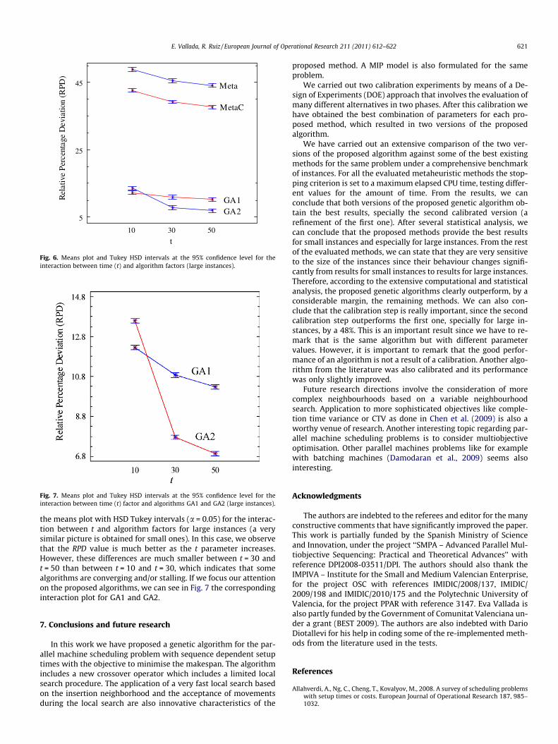
t

GA2GA1

MetaC

Meta

5

25

45

10 30 50

Rel

ativ

e P

erce

ntag

e D

evia

tion

(RPD

)

Fig. 6. Means plot and Tukey HSD intervals at the 95% confidence level for theinteraction between time (t) and algorithm factors (large instances).

Fig. 7. Means plot and Tukey HSD intervals at the 95% confidence level for theinteraction between time (t) factor and algorithms GA1 and GA2 (large instances).

E. Vallada, R. Ruiz / European Journal of Operational Research 211 (2011) 612–622 621

the means plot with HSD Tukey intervals (a = 0.05) for the interac-tion between t and algorithm factors for large instances (a verysimilar picture is obtained for small ones). In this case, we observethat the RPD value is much better as the t parameter increases.However, these differences are much smaller between t = 30 andt = 50 than between t = 10 and t = 30, which indicates that somealgorithms are converging and/or stalling. If we focus our attentionon the proposed algorithms, we can see in Fig. 7 the correspondinginteraction plot for GA1 and GA2.

7. Conclusions and future research

In this work we have proposed a genetic algorithm for the par-allel machine scheduling problem with sequence dependent setuptimes with the objective to minimise the makespan. The algorithmincludes a new crossover operator which includes a limited localsearch procedure. The application of a very fast local search basedon the insertion neighborhood and the acceptance of movementsduring the local search are also innovative characteristics of the

proposed method. A MIP model is also formulated for the sameproblem.

We carried out two calibration experiments by means of a De-sign of Experiments (DOE) approach that involves the evaluation ofmany different alternatives in two phases. After this calibration wehave obtained the best combination of parameters for each pro-posed method, which resulted in two versions of the proposedalgorithm.

We have carried out an extensive comparison of the two ver-sions of the proposed algorithm against some of the best existingmethods for the same problem under a comprehensive benchmarkof instances. For all the evaluated metaheuristic methods the stop-ping criterion is set to a maximum elapsed CPU time, testing differ-ent values for the amount of time. From the results, we canconclude that both versions of the proposed genetic algorithm ob-tain the best results, specially the second calibrated version (arefinement of the first one). After several statistical analysis, wecan conclude that the proposed methods provide the best resultsfor small instances and especially for large instances. From the restof the evaluated methods, we can state that they are very sensitiveto the size of the instances since their behaviour changes signifi-cantly from results for small instances to results for large instances.Therefore, according to the extensive computational and statisticalanalysis, the proposed genetic algorithms clearly outperform, by aconsiderable margin, the remaining methods. We can also con-clude that the calibration step is really important, since the secondcalibration step outperforms the first one, specially for large in-stances, by a 48%. This is an important result since we have to re-mark that is the same algorithm but with different parametervalues. However, it is important to remark that the good perfor-mance of an algorithm is not a result of a calibration. Another algo-rithm from the literature was also calibrated and its performancewas only slightly improved.

Future research directions involve the consideration of morecomplex neighbourhoods based on a variable neighbourhoodsearch. Application to more sophisticated objectives like comple-tion time variance or CTV as done in Chen et al. (2009) is also aworthy venue of research. Another interesting topic regarding par-allel machine scheduling problems is to consider multiobjectiveoptimisation. Other parallel machines problems like for examplewith batching machines (Damodaran et al., 2009) seems alsointeresting.

Acknowledgments

The authors are indebted to the referees and editor for the manyconstructive comments that have significantly improved the paper.This work is partially funded by the Spanish Ministry of Scienceand Innovation, under the project ‘‘SMPA – Advanced Parallel Mul-tiobjective Sequencing: Practical and Theoretical Advances’’ withreference DPI2008-03511/DPI. The authors should also thank theIMPIVA – Institute for the Small and Medium Valencian Enterprise,for the project OSC with references IMIDIC/2008/137, IMIDIC/2009/198 and IMIDIC/2010/175 and the Polytechnic University ofValencia, for the project PPAR with reference 3147. Eva Vallada isalso partly funded by the Government of Comunitat Valenciana un-der a grant (BEST 2009). The authors are also indebted with DarioDiotallevi for his help in coding some of the re-implemented meth-ods from the literature used in the tests.

References

Allahverdi, A., Ng, C., Cheng, T., Kovalyov, M., 2008. A survey of scheduling problemswith setup times or costs. European Journal of Operational Research 187, 985–1032.

622 E. Vallada, R. Ruiz / European Journal of Operational Research 211 (2011) 612–622

Anghinolfi, D., Paolucci, M., 2007. Parallel machine total tardiness scheduling with anew hybrid metaheuristic approach. Computers & Operations Research 34,3471–3490.

Armentano, V., Felizardo, M., 2007. Minimizing total tardiness in parallel machinescheduling with setup times: An adaptive memory-based GRASP approach.European Journal of Operational Research 183, 100–114.

Chen, J., 2005. Unrelated parallel machine scheduling with secondary resourceconstraints. International Journal of Advanced Manufacturing Technology 26,285–292.

Chen, J., 2006. Minimization of maximum tardiness on unrelated parallel machineswith process restrictions and setups. International Journal of AdvancedManufacturing Technology 29, 557–563.

Chen, J., Wu, T., 2006. Total tardiness minimization on unrelated parallel machinescheduling with auxiliary equipment constraints. OMEGA, The InternationalJournal of Management Science 34, 81–89.

Chen, Y.R., Li, X.P., Sawhney, R., 2009. Restricted job completion time varianceminimisation on identical parallel machines. European Journal of IndustrialEngineering 3 (3), 261–276.

Damodaran, P., Hirani, N.S., Velez-Gallego, M.C., 2009. Scheduling identical parallelbatch processing machines to minimise makespan using genetic algorithms.European Journal of Industrial Engineering 3 (2), 187–206.

Dunstall, S., Wirth, A., 2005. Heuristic methods for the identical parallel machineflowtime problem with set-up times. Computers & Operations Research 32,2479–2491.

Eom, D., Shin, H., Kwun, I., Shim, J., Kim, S., 2002. Scheduling jobs on parallelmachines with sequence dependent family set-up times. International Journalof Advanced Manufacturing Technology 19, 926–932.

Franca, P., Gendreau, M., Laporte, G., Mnller, F., 1996. A tabu search heuristic for themultiprocessor scheduling problem with sequence dependent setup times.International Journal of Production Economics 43, 79–89.

Gendreau, M., Laporte, G., Morais-Guimaraes, E., 2001. A divide and merge heuristicfor the multiprocessor scheduling problem with sequence dependent setuptimes. European Journal of Operational Research 133, 183–189.

Goldberg, D.E., 1989. Genetic Algorithms in Search, Optimization and MachineLearning. Addison-Wesley, Reading.

Guinet, A., 1993. Scheduling sequence-dependent jobs on identical parallelmachines to minimize completion time criteria. International Journal ofProduction Research 31, 1579–1594.

Holland, J.H., 1975. Adaptation in Natural and Artificial Systems. The University ofMichigan Press, Ann Arbor.

Hurink, J., Knust, S., 2001. List scheduling in a parallel machine environment withprecedence constraints and setup times. Operations Research Letters 29, 231–239.

Kim, C., Shin, H., 2003. Scheduling jobs on parallel machines: a restricted tabusearch approach. International Journal of Advanced Manufacturing Technology22, 278–287.

Kim, D., Kim, K., Jang, W., Chen, F., 2002. Unrelated parallel machine schedulingwith setup times using simulated annealing. Robotics and Computer IntegratedManufacturing 18, 223–231.

Kim, D., Na, D., Chen, F., 2003. Unrelated parallel machine scheduling with setuptimes and a total weighted tardiness objective. Robotics and ComputerIntegrated Manufacturing 19, 173–181.

Kurz, M., Askin, R., 2001. Heuristic scheduling of parallel machines with sequence-dependent set-up times. International Journal of Production Research 39, 3747–3769.

Lee, Y., Pinedo, M., 1997. Scheduling jobs on parallel machines with sequence-dependent setup times. European Journal of Operational Research 100, 464–474.

Logendran, R., McDonell, B., Smucker, B., 2007. Scheduling unrelated parallelmachines with sequence-dependent setups. Computers & Operations Research34, 3420–3438.

Low, C., 2005. Simulated annealing heuristic for flow shop scheduling problemswith unrelated parallel machines. Computers & Operations Research 32, 2013–2025.

Montgomery, D., 2007. Design and Analysis of Experiments, fifth ed. John Wiley &Sons, New York.

Pfund, M., Fowler, J., Gadkari, A., Chen, Y., 2008. Scheduling jobs on parallelmachines with setup times and ready times. Computers & IndustrialEngineering 54, 764–782.

Pinedo, M., 2008. Scheduling: Theory, Algorithms and Systems, third ed. PrenticeHall, New Jersey.

Rabadi, G., Moraga, R., Salem, A., 2006. Heuristics for the unrelated parallel machinescheduling problem with setup times. Journal of Intelligent Manufacturing 17,85–97.

Rocha de Paula, M., Gómez-Ravetti, M., Robson-Mateus, G., Pardalos, P., 2007.Solving parallel machines scheduling problems with sequence-dependent setuptimes using variable neighbourhood search. IMA, Journal of ManagementMathematics 18, 101–115.

Ruiz, R., Allahverdi, A., 2007. No-wait flowshop with separate setup times tominimize maximum lateness. International Journal of Advanced ManufacturingTechnology 35 (5–6), 551–565.

Ruiz, R., Maroto, C., Alcaraz, J., 2006. Two new robust genetic algorithms for theflowshop scheduling problem. OMEGA, The International Journal ofManagement Science 34, 461–476.

Tahar, D., Yalaoui, F., Chu, C., Amodeo, L., 2006. A linear programming approach foridentical parallel machine scheduling with job splitting and sequence-dependent setup times. International Journal of Production Economics 99,63–73.

Weng, M., Lu, J., Ren, H., 2001. Unrelated parallel machine scheduling with setupconsideration and a total weighted completion time objective. InternationalJournal of Production Economics 70, 215–226.