Embed Size (px)
Citation preview
A GENETIC ALGORITHM FOR THE WEIGHT SETTING
PROBLEM IN OSPF ROUTING
M. ERICSSON, M.G.C. RESENDE, AND P.M. PARDALOS
Abstract. With the growth of the Internet, Internet Service Providers (ISPs)try to meet the increasing traffic demand with new technology and improvedutilization of existing resources. Routing of data packets can affect networkutilization. Packets are sent along network paths from source to destinationfollowing a protocol. Open Shortest Path First (OSPF) is the most commonlyused intra-domain Internet routing protocol (IRP). Traffic flow is routed alongshortest paths, splitting flow at nodes with several outgoing links on a shortestpath to the destination IP address. Link weights are assigned by the networkoperator. A path length is the sum of the weights of the links in the path.The OSPF weight setting (OSPFWS) problem seeks a set of weights thatoptimizes network performance. We study the problem of optimizing OSPFweights, given a set of projected demands, with the objective of minimizingnetwork congestion. The weight assignment problem is NP-hard. We presenta genetic algorithm (GA) to solve the OSPFWS problem. We compare ourresults with the best known and commonly used heuristics for OSPF weightsetting, as well as with a lower bound of the optimal multi-commodity flowrouting, which is a linear programming relaxation of the OSPFWS problem.Computational experiments are made on the AT&T Worldnet backbone withprojected demands, and on twelve instances of synthetic networks.
1. Introduction
With the growth of the Internet, traffic is approximately doubling each year [8].Today, Internet Service Providers (ISPs) try to meet tomorrow’s escalating trafficdemand with new technologies, but primarily with a massive capacity expansion ofalready existing links. There have been spectacular growth rates of traffic, doublingevery three months in the 1995–96 boom, caused by the emerging graphic-intensiveweb browsers. In 2000, the growth rate has recessed to doubling each year. In thenear future, we are likely to see another data traffic boom due to the worldwidespread of the Internet and its use for an increasing number of purposes. Thesedevelopments highlight the importance of Internet traffic engineering, which seeksmore efficient use of existing network resources.
The Internet on a network level is built up of approximately twelve major InternetService Providers (ISPs) worldwide [25]. An ISP is a company that provides accessto the Internet and lets other companies lease bandwidth from their high-speedlines. AT&T Worldnet is an example of a large ISP. The larger ISPs arrangepeering agreements to exchange traffic. Connected to these major backbones arethe regional providers with thousands of local providers. Individual users can alsoget access through online service providers.
Date: October 9, 2001.Key words and phrases. OSPF routing, Internet, metaheuristics, genetic algorithm, path
relinking.1
2 M. ERICSSON, M.G.C. RESENDE, AND P.M. PARDALOS
When one sends or receives data over the Internet, the information is dividedinto small chunks called packets or datagrams. A header, containing the necessarytransmission information, such as the destination Internet Protocol (IP) address, isattached to each packet. The data packets are sent along links between routers onInternet. When a data packet reaches a router, the incoming datagrams are storedin a queue to await processing. The router reads the datagram header, takes theIP destination address and determines the best way to forward this packet for itto reach its final destination [4]. As each packet is treated individually, the orderin which they arrive may not be the same order in which they were sent out. TheInternet Protocol (IP) simply delivers them and it is up to the Transmission ControlProtocol (TCP) to reorder the datagrams.
Routing is a fundamental engineering task on the Internet. It consists in findinga path from a source to a destination host. Routing is complex in large networksbecause of the many potential intermediate destinations a packet might traversebefore reaching its destination [26]. To decrease complexity, the network is dividedinto smaller domains. Considering each domain individually makes the networkmore manageable. Routing domains in today’s Internet are called autonomoussystems (AS). Interior Gateway Protocols (IGP) are used within the AS, whileExterior Gateway Protocols (EGP) are used to route traffic flow between them [4].
The TCP/IP suite has many routing protocols, such as OSPF, BGP, RIP, IGRP,and Integrated IS-IS, all in use in today’s Internet [4, 23]. OSPF, RIP, IGRP, andIS-IS are categorized as IGPs, while BGP is an EGP. A routing table instructs therouter how to forward packets. The routing protocols employ different operations toanalyze different incoming update messages to produce their routing tables. Givena packet with an IP destination address in its header, the router performs a routingtable lookup which returns the IP address of the packet’s next hop.
Open Shortest Path First (OSPF) is the most commonly used intra-domain In-ternet routing protocol [12, 26]. OSPF requires routers to exchange routing infor-mation with all other routers in the AS. Complete network topology knowledge, i.e.the arrangement of all routers and links in the domain, is required. Because eachrouter knows the complete topology, each router can compute all needed shortestpaths [4]. OSPF is a dynamic protocol and quickly detects topological changes inthe AS and calculates new loop-free routes after a short period of convergence [16].
OSPF calculates routes as follows. Each link is assigned a dimensionless metric,called cost or weight. This integer cost ranges from 1 to 65535 (= 216 − 1) and isshown in the link-state database. The cost of a path in the directed graph is thesum of the link costs. Using Dijkstra’s shortest path algorithm [9], OSPF mandatesthat each router computes a tree of shortest paths with itself as the root [16]. Thistree shows the best routes to all destinations in the AS. The destination router inthe first hop is extracted into the IP routing table. In the case of multiple shortestpaths, some vendors have implemented OSPF so that it will use load balancing andsplit the traffic flow over several shortest paths [23].
The link weights are assigned by the network operator. The lower the weight, thegreater the chance that traffic will get routed on that link [4]. Recommendationshave been suggested as to how to assign link weights. Cisco, a major router vendor,by default, assigns OSPF metrics as the inverse of the interface available bandwidth[26]. If each link cost is set to 1, the cost of a path is equal to the number of links(hops) in the path [23]. In this paper, we propose a technique to find good OSPF
A GA FOR WEIGHT SETTING IN OSPF ROUTING 3
routing weight settings for a given network and router-to-router traffic requirements(demand).
OSPF is an IGP and, therefore, is designed to run internal to a single AS. Thereare evolving guidelines on how to best design an OSPF network. In 1991, theguideline was at most 200 routers in a single area [22]. To date, Cisco’s guidelinerecommends no more than six router hops from source to destination, and 30 to100 routers per area [26]. There is no limit in the number of routers per area, butfor OSPF to scale well, less than 40 routers in an area is recommended [26]. AsOSPF uses a CPU-intensive shortest-path algorithm, experience has shown that40 to 50 routers per area is the optimal upper limit for OSPF. Our test problemsrange very realistically from 50 routers (148 links) to 100 routers (503 links). Ouronly real-world network is a realistic version of the AT&T Worldnet backbone. Theinstance we use is a few years old and has 90 routers and 274 links.
The mathematical model of a data communications network is the general rout-ing problem, defined as follows. Consider the capacitated directed graph G =(N,A, c), A ∈ N ×N, c : A → �
, where N and A denote, respectively, the sets ofnodes and arcs. The nodes and arcs represent routers and the capacitated networklinks, respectively. Given the demand matrix D = (dst), with origin-destinationpairs (s, t), where dst is the amount of data traffic to be sent from IP source ad-dress s to IP target address t, the problem is to route this demand on paths in thenetwork while minimizing congestion.
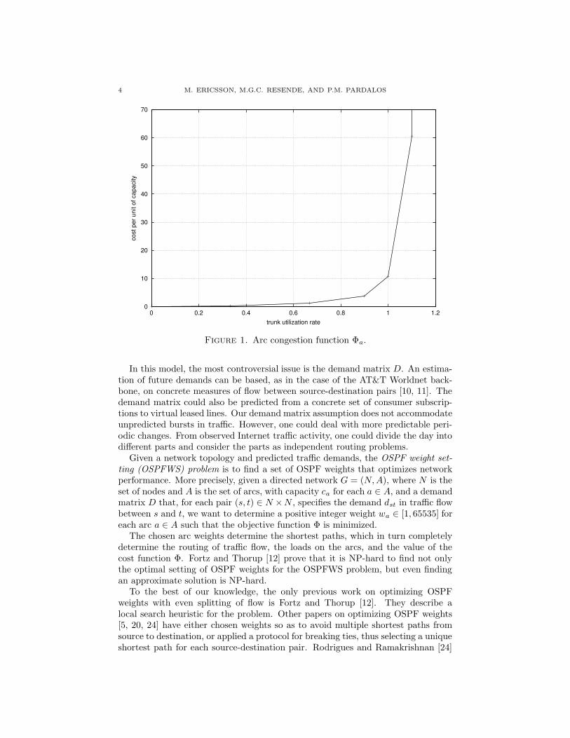
We use the congestion measure proposed by Fortz and Thorup [12]. With eacharc a ∈ A, we associate a cost Φa as a function of the utilization la/ca, i.e. howclose the load la is to the link capacity ca. Our objective is to distribute the flowso as to minimize the sum of the costs over all arcs
Φ =∑
a∈AΦa(la).(1)
Generally, Φ favors sending flow over arcs with small utilization. The cost in-creases progressively as the utilization approaches 100% and then explodes whenmaximum capacity is reached. This approach of heavily penalizing congestion givesus our formal objective.
The cost function Φ is piecewise linear and convex. For each arc a ∈ A, Φa isthe continuous function with Φa(0) = 0 and derivative
Φ′a(la) =
1 for 0 ≤ la/ca < 1/3,3 for 1/3 ≤ la/ca < 2/3,
10 for 2/3 ≤ la/ca < 9/10,70 for 9/10 ≤ la/ca < 1,
500 for 1 ≤ la/ca < 11/10,5000 for 11/10 ≤ la/ca < ∞.
(2)
Function Φa is depicted in Figure 1. Because of the explosive increase in cost asloads exceed capacities, our objective is to keep the maximum utilization maxa∈A la/cabelow 1, if possible.
In the general routing problem, there are no constraints on how flow can bedistributed along the paths, and the problem can be formulated and solved inpolynomial time as a multi-commodity flow problem. Other choices of the objectivefunction are possible, see e.g. Awduche et al. [2].
4 M. ERICSSON, M.G.C. RESENDE, AND P.M. PARDALOS
0
10
20
30
40
50
60
70
0 0.2 0.4 0.6 0.8 1 1.2
cost
per
uni
t of c
apac
ity
trunk utilization rate
Figure 1. Arc congestion function Φa.
In this model, the most controversial issue is the demand matrix D. An estima-tion of future demands can be based, as in the case of the AT&T Worldnet back-bone, on concrete measures of flow between source-destination pairs [10, 11]. Thedemand matrix could also be predicted from a concrete set of consumer subscrip-tions to virtual leased lines. Our demand matrix assumption does not accommodateunpredicted bursts in traffic. However, one could deal with more predictable peri-odic changes. From observed Internet traffic activity, one could divide the day intodifferent parts and consider the parts as independent routing problems.
Given a network topology and predicted traffic demands, the OSPF weight set-ting (OSPFWS) problem is to find a set of OSPF weights that optimizes networkperformance. More precisely, given a directed network G = (N,A), where N is theset of nodes and A is the set of arcs, with capacity ca for each a ∈ A, and a demandmatrix D that, for each pair (s, t) ∈ N ×N , specifies the demand dst in traffic flowbetween s and t, we want to determine a positive integer weight wa ∈ [1, 65535] foreach arc a ∈ A such that the objective function Φ is minimized.
The chosen arc weights determine the shortest paths, which in turn completelydetermine the routing of traffic flow, the loads on the arcs, and the value of thecost function Φ. Fortz and Thorup [12] prove that it is NP-hard to find not onlythe optimal setting of OSPF weights for the OSPFWS problem, but even findingan approximate solution is NP-hard.
To the best of our knowledge, the only previous work on optimizing OSPFweights with even splitting of flow is Fortz and Thorup [12]. They describe alocal search heuristic for the problem. Other papers on optimizing OSPF weights[5, 20, 24] have either chosen weights so as to avoid multiple shortest paths fromsource to destination, or applied a protocol for breaking ties, thus selecting a uniqueshortest path for each source-destination pair. Rodrigues and Ramakrishnan [24]
A GA FOR WEIGHT SETTING IN OSPF ROUTING 5
present a local search procedure similar to that of Fortz and Thorup. They con-sider only a single descent and work with small networks having at most 16 nodesand 18 links. Bley et al. [5] use local search with single descent and considersmall networks with at most 13 links. They simultaneously deal with the problemof designing the network. Lin and Wang [20] present a completely different ap-proach based on Lagrangian relaxation, and consider networks up to 26 nodes. Wetested our algorithm on the test problems used by Fortz and Thorup. The AT&TWorldnet backbone, as well as the other test problems, are described in Section 4.
In this paper, we present a genetic algorithm, which we call GAOSPF, for op-timizing OSPF weights for intra-domain Internet routing. We use similar objec-tive, modeling of the OSPFWS problem, and measure of algorithm performanceas Fortz and Thorup. GAOSPF is tested on the AT&T Worldnet backbone, aswell as on twelve instances of synthetic networks, from three different theoreticalnetwork models. Results are compared to a linear programming (LP) relaxationlower bound and to other commonly used heuristics for weight setting. We alsocompare our results with the local search heuristic of Fortz and Thorup [12]. Formost network instances, GAOSPF finds solutions within a few percent of the LPlower bound. Compared to the commonly used heuristic recommended by Cisco,we are able to increase network capacity by 70% for the AT&T Worldnet back-bone, and over 100% for the most realistic 2-level hierarchical graphs before thenetwork becomes congested. The average possible traffic increase is 52% for all testproblems.
2. Mathematical formulation
In a data communication network, nodes and arcs represent routers and trans-mission links, respectively. Let N and A denote, respectively, the sets of nodesand arcs. Data packets are routed along links, which have fixed capacities. In theOSPFWS problem, we relax the capacity constraint and penalize congestion witha cost function Φ, defined in (1). Each demand from source to destination routerrepresents a commodity. This way, the problem of determining the minimum costrouting of all demands is an uncapacitated multicommodity flow problem [1].
Given a directed network graph G = (N,A) with a capacity ca for each a ∈ A,and a demand matrix D that, for each pair (s, t) ∈ N ×N , gives the demand dstin traffic flow between nodes s and t, then for each pair (s, t) and each arc a, we
associate a variable f(st)a that indicates how much of the traffic flow from s to t
goes over a. Variable la represents the total load on arc a, i.e. the sum of the flowsgoing over a, and Φa is used to model the piecewise linear cost function of arc a[12].
With this notation, the multi-commodity flow problem with increasing linearcosts is formulated as the following linear program:
min Φ =∑
a∈AΦa
6 M. ERICSSON, M.G.C. RESENDE, AND P.M. PARDALOS
subject to
∑
u:(u,v)∈Af
(st)(u,v) −
∑
u:(v,u)∈Af
(st)(v,u) =
−dst if v = s,dst if v = t,0 otherwise,
v, s, t ∈ N,(3)
la =∑
(s,t)∈N×Nf (st)a , a ∈ A,(4)
Φa ≥ la, a ∈ A,(5)
Φa ≥ 3la − 2/3ca, a ∈ A,(6)
Φa ≥ 10la − 16/3ca, a ∈ A,(7)
Φa ≥ 70la − 178/3ca, a ∈ A,(8)
Φa ≥ 500la − 1468/3ca, a ∈ A,(9)
Φa ≥ 5000la − 19468/3ca, a ∈ A,(10)
f (st)a ≥ 0, a ∈ A; s, t ∈ N.(11)
Constraints (3) are flow conservation constraints that ensure routing of the de-sired traffic. Constraints (4) define the load on each arc and constraints (5–10)define the cost on each arc according to the cost function Φ.
This linear program is a relaxation of OSPF routing, as it allows for arbitrarysplitting of flow. It can be solved optimally in polynomial time [17, 18]. In ourcomputational experiments, we solve this LP relaxation optimally to obtain a lowerbound of the optimal OSPFWS solution. We denote this lower bound by LPLB.
Fortz and Thorup [12] show that the largest gap between LPLB and the valueof an optimal solution of the OSPFWS problem is at most 5000. They show that,for a specific family of networks, this gap can approach 5000.
3. GA for the OSPFWS problem
Genetic algorithms (GA) are global optimization techniques derived from theprinciples of natural selection and evolutionary theory [13, 14]. Genetic algorithmshave been theoretically and empirically proven to be robust search techniques [13].Each possible point in the search space of the problem is encoded into a represen-tation suitable for applying the GA. A GA transforms a population of individualsolutions, each with an associated fitness (or objective function value), into a newgeneration of the population, using the Darwinian principle of survival of the fittest.By applying genetic operators, such as crossover and mutation, a GA successivelyproduces better approximations to the solution. At each iteration, a new generationof approximations is created by the process of selection and reproduction [19].
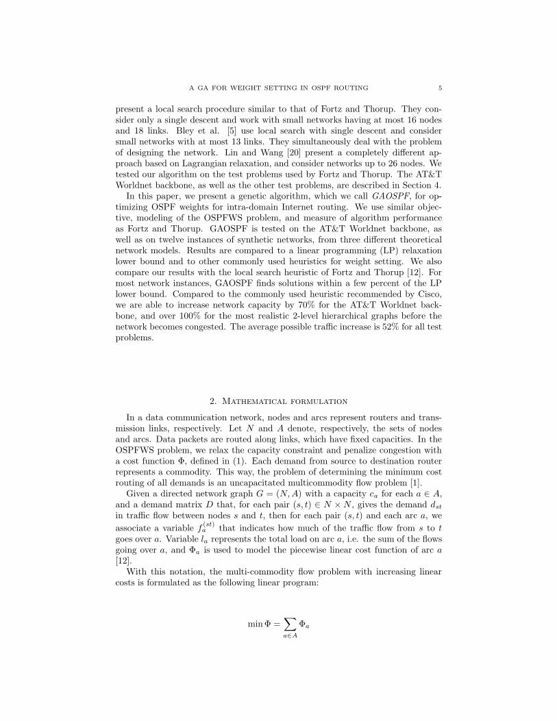
A simple genetic algorithm is described by the pseudo-code in Figure 2. In thispseudo-code, the population at time t is represented by P (t).
The three steps of a GA, according to the pseudo code, are:
1. Randomly create an initial population P (0) of individuals.2. Iteratively perform the following substeps on the current generation of the
population until the termination criterion has been satisfied.(a) Assign fitness value to each individual using the fitness function.(b) Select parents to mate.(c) Create children from selected parents by crossover and mutation.(d) Identify the best-so-far individual for this iteration of the GA.
A GA FOR WEIGHT SETTING IN OSPF ROUTING 7
begint = 0initialize P (0)evaluate P (0)while(not termination-criteria) do
t = t+ 1select P (t) from P (t− 1)alter P (t)evaluate P (t)
endend
Figure 2. Pseudo-code for a simple genetic algorithm
3.1. Implementation of GA for the OSPFWS problem. Next, we describehow the above principles were tailored to produce a genetic algorithm for theOSPFWS problem.
3.1.1. Representation. Since the representation of a solution should be such thatthe genetic operators produce feasible offsprings, encoding is often difficult whentailoring a genetic algorithm for an optimization problem. However, this is not thecase for the OSPFWS problem. A solution to the OSPFWS problem is representedby a point in the discrete search space [1, 65535]|A|. We used the representation ofweights w = 〈w1, w2, . . . , w|A|〉, where wi ∈ [1, 65535] for each arc i = 1, . . . , |A|.All points in the search space represent feasible solutions. As we note later, insteadof using the upper limit of 65535, in our implementation we use a user-definedupper limit MAXWEIGHT.
3.1.2. Initial population. The initial population is generated by randomly choosingfeasible points in the search space [1, 65535]|A|, represented as integer vectors. Inaddition to these randomly generated solutions, we also add the weight settings oftwo other common heuristics. We add UnitOSPF , represented by the unit vector,and InvCapOSPF , represented by the weight vector where each arc weight is setinversely proportional to its arc capacity. Both heuristics are described later.
3.1.3. Evaluation function. The association of each solution to a fitness value isdone through the fitness function. We associate a cost to each individual throughthe cost function Φ. The evaluation function is complex and computationally de-manding, as it includes the process of OSPF routing, needed to determine the arcloads resulting from a given set of weights. This evaluation function is the com-putational bottleneck of the algorithm. Another basic computation needed by thegenetic algorithm is the comparison of different solutions. The fitness value is thesame as the cost value. In other words, “cost” and “fitness” are used in the samesense, i.e. less fitness is better. We now show how we calculate the cost function Φfor a given weight setting {wa}a∈A, and a given graph G = (N,A) with capacities{ca}a∈A, and demands dst ∈ D. We follow closely the procedure given in Fortz andThorup [12].
A given weight setting will completely determine the shortest paths, which inturn determine the OSPF routing, and how much of the demand is sent over which
8 M. ERICSSON, M.G.C. RESENDE, AND P.M. PARDALOS
arcs. The load on each arc gives us the arc utilization, which in turn gives us acost from the cost function Φa. The total cost Φ for all arcs in the network is thefitness value.
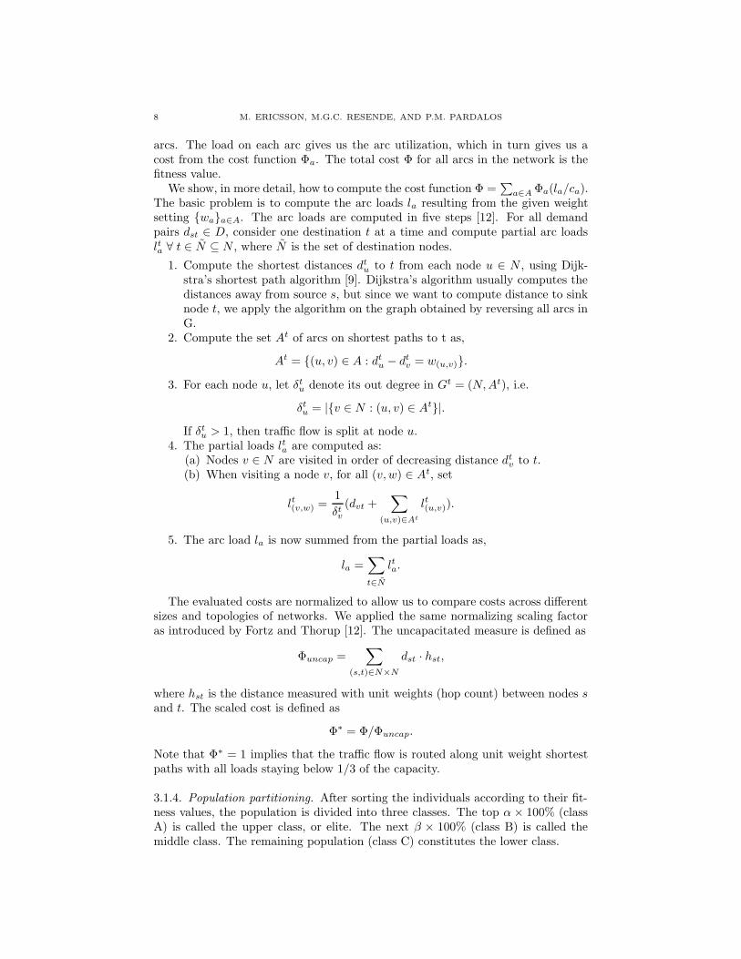
We show, in more detail, how to compute the cost function Φ =∑a∈A Φa(la/ca).
The basic problem is to compute the arc loads la resulting from the given weightsetting {wa}a∈A. The arc loads are computed in five steps [12]. For all demandpairs dst ∈ D, consider one destination t at a time and compute partial arc loadslta ∀ t ∈ N ⊆ N , where N is the set of destination nodes.
1. Compute the shortest distances dtu to t from each node u ∈ N , using Dijk-stra’s shortest path algorithm [9]. Dijkstra’s algorithm usually computes thedistances away from source s, but since we want to compute distance to sinknode t, we apply the algorithm on the graph obtained by reversing all arcs inG.
2. Compute the set At of arcs on shortest paths to t as,
At = {(u, v) ∈ A : dtu − dtv = w(u,v)}.
3. For each node u, let δtu denote its out degree in Gt = (N,At), i.e.
δtu = |{v ∈ N : (u, v) ∈ At}|.If δtu > 1, then traffic flow is split at node u.
4. The partial loads lta are computed as:(a) Nodes v ∈ N are visited in order of decreasing distance dtv to t.(b) When visiting a node v, for all (v, w) ∈ At, set
lt(v,w) =1
δtv(dvt +
∑
(u,v)∈Atlt(u,v)).
5. The arc load la is now summed from the partial loads as,
la =∑
t∈Nlta.
The evaluated costs are normalized to allow us to compare costs across differentsizes and topologies of networks. We applied the same normalizing scaling factoras introduced by Fortz and Thorup [12]. The uncapacitated measure is defined as
Φuncap =∑
(s,t)∈N×Ndst · hst,
where hst is the distance measured with unit weights (hop count) between nodes sand t. The scaled cost is defined as
Φ∗ = Φ/Φuncap.
Note that Φ∗ = 1 implies that the traffic flow is routed along unit weight shortestpaths with all loads staying below 1/3 of the capacity.
3.1.4. Population partitioning. After sorting the individuals according to their fit-ness values, the population is divided into three classes. The top α × 100% (classA) is called the upper class, or elite. The next β × 100% (class B) is called themiddle class. The remaining population (class C) constitutes the lower class.
A GA FOR WEIGHT SETTING IN OSPF ROUTING 9
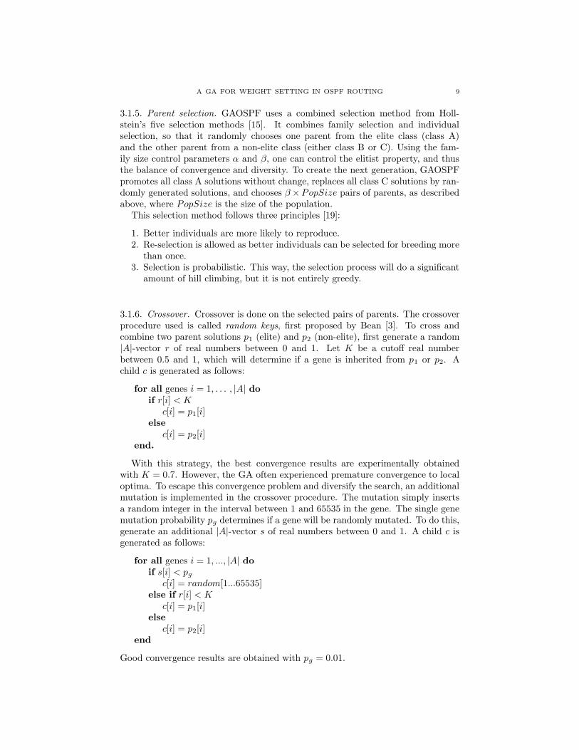
3.1.5. Parent selection. GAOSPF uses a combined selection method from Holl-stein’s five selection methods [15]. It combines family selection and individualselection, so that it randomly chooses one parent from the elite class (class A)and the other parent from a non-elite class (either class B or C). Using the fam-ily size control parameters α and β, one can control the elitist property, and thusthe balance of convergence and diversity. To create the next generation, GAOSPFpromotes all class A solutions without change, replaces all class C solutions by ran-domly generated solutions, and chooses β ×PopSize pairs of parents, as describedabove, where PopSize is the size of the population.
This selection method follows three principles [19]:
1. Better individuals are more likely to reproduce.2. Re-selection is allowed as better individuals can be selected for breeding more
than once.3. Selection is probabilistic. This way, the selection process will do a significant
amount of hill climbing, but it is not entirely greedy.
3.1.6. Crossover. Crossover is done on the selected pairs of parents. The crossoverprocedure used is called random keys, first proposed by Bean [3]. To cross andcombine two parent solutions p1 (elite) and p2 (non-elite), first generate a random|A|-vector r of real numbers between 0 and 1. Let K be a cutoff real numberbetween 0.5 and 1, which will determine if a gene is inherited from p1 or p2. Achild c is generated as follows:
for all genes i = 1, . . . , |A| doif r[i] < K
c[i] = p1[i]else
c[i] = p2[i]end.
With this strategy, the best convergence results are experimentally obtainedwith K = 0.7. However, the GA often experienced premature convergence to localoptima. To escape this convergence problem and diversify the search, an additionalmutation is implemented in the crossover procedure. The mutation simply insertsa random integer in the interval between 1 and 65535 in the gene. The single genemutation probability pg determines if a gene will be randomly mutated. To do this,generate an additional |A|-vector s of real numbers between 0 and 1. A child c isgenerated as follows:
for all genes i = 1, ..., |A| doif s[i] < pg
c[i] = random[1...65535]else if r[i] < K
c[i] = p1[i]else
c[i] = p2[i]end
Good convergence results are obtained with pg = 0.01.
10 M. ERICSSON, M.G.C. RESENDE, AND P.M. PARDALOS
4. Computational results
We describe computational experiments with a C language implementation ofGAOSPF. The genetic algorithm is compared with several heuristics as well as thelinear programming lower bound. Most of the experiments were done on an IBMSP RS6000 system, running AIX v4.3. An additional experiment was done on anSGI Challenge computer (196-MHz MIPS R10000).
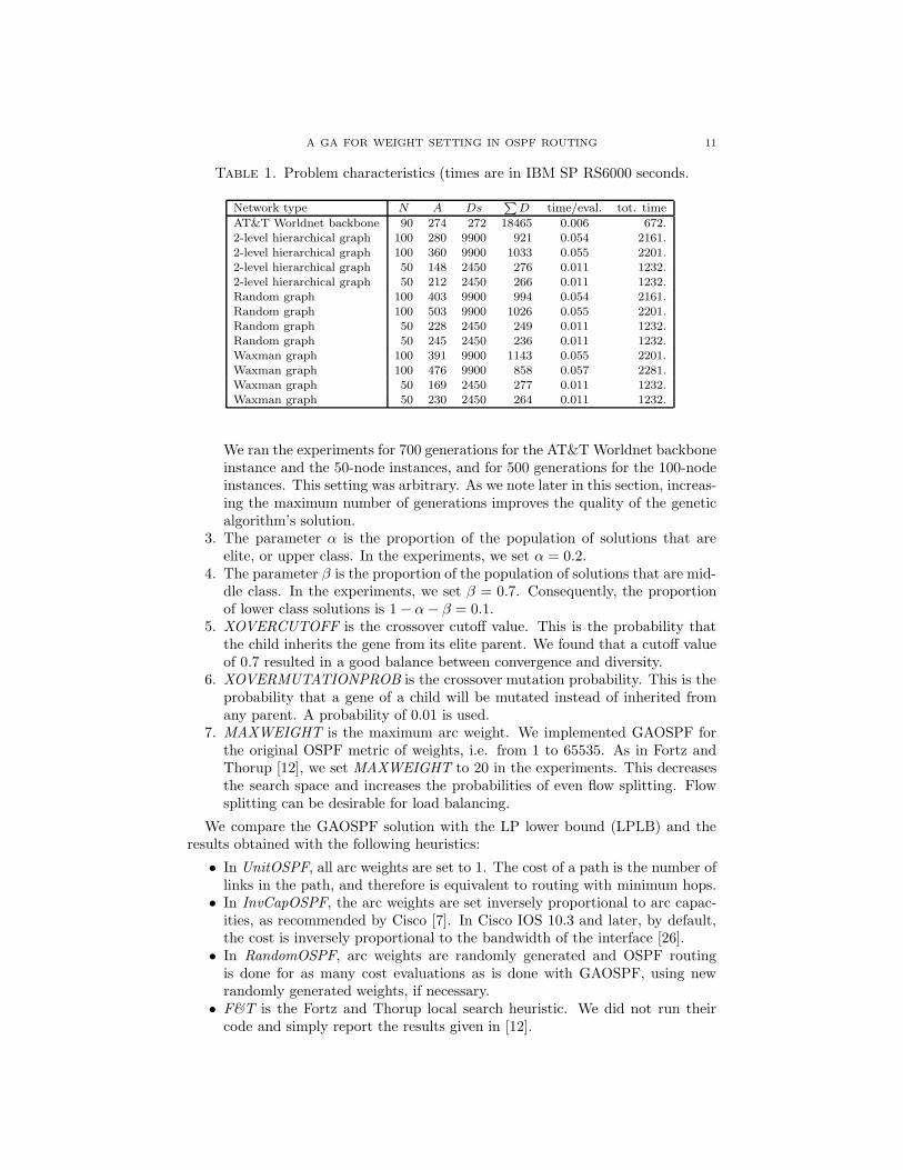
The objective of the experiments was to study the performance of the geneticalgorithm on the test problems used in Fortz and Thorup [12]. These problems con-sist of instances on the AT&T Worldnet backbone network with projected demands,and three flavors of synthetic networks. Problem characteristics are summarized inTable 1. For each problem, the table lists its type, number of nodes (N), number ofarcs (A), number of demand pairs (Ds), sum of demands (
∑D), time (in seconds)
to make one cost evaluation, and product of time for a single cost evaluation (timeeval.) and the total number of evaluations made in the experiments (tot. time).
The AT&T Worldnet backbone is a real-world network of 90 routers and 274links. The 2-level hierarchical networks are generated using the GT-ITM generator[28], based on a model of Calvert et al. [6] and Zegura et al. [29]. Arcs are of twotypes. Local access arcs have capacities equal to 200, while long distance arcs havecapacities equal to 1000. For the random networks, the probability of having an arcbetween two nodes is given by a constant parameter that controls the density of thenetwork. All arc capacities are set to 1000. In the Waxman networks, the nodesare points uniformly distributed in the unit square. The probability of having anarc between nodes u and v is ηe−δ(u,v)/(2θ), where η is a parameter used to controlthe density of the network, δ(u, v) is the Euclidean distance between u and v, andθ is the maximum distance between any two nodes in the network [27]. All arccapacities are set to 1000. Fortz and Thorup generated the demands to force somenodes to be more active senders or receivers than others, thus modeling hot spotson the network. Their generation assigns higher demands to closely located nodespairs. Details can be found in [12].
The cost evaluation of a solution is the computational bottleneck of the al-gorithm. The cost evaluation includes the shortest path evaluations, as well asthe OSPF routing. Recall that in Table 1, the average time (time/eval.), in sec-onds, for each cost evaluation is listed. For example, the total expected runningtime for a run with population size (PopSize) of 200, maximum number of gen-erations (MaxGen) of 700, and elite population parameter α of 0.2, results in(1− α)× PopSize× (MaxGen− 1) + PopSize = 112040 cost evaluations. Underthese parameter settings, on the AT&T Worldnet backbone network, the algorithmwill run for approximately 672 seconds on the IBM SP RS6000 system.
GAOSPF requires that seven parameters be specified:
1. POPSIZE denotes the size of the population. This variable affects the runningtime of the GA. We ran tests with moderate population sizes of 50 up to 500.In the experiments, we set POPSIZE to 200 for the AT&T Worldnet backboneinstance and all 50-node instances, and to 100 for all 100-node instances. Thissetting was arbitrary. Increasing population size usually improves the qualityof the genetic algorithm’s solution.
2. MAXGEN denotes the number of generations. The genetic algorithm usesthis parameter as a stopping criterion. GAOSPF finds good solutions afteronly about 100 generations, but continues to find improvements afterwards.
A GA FOR WEIGHT SETTING IN OSPF ROUTING 11
Table 1. Problem characteristics (times are in IBM SP RS6000 seconds.
Network type N A Ds∑D time/eval. tot. time
AT&T Worldnet backbone 90 274 272 18465 0.006 672.2-level hierarchical graph 100 280 9900 921 0.054 2161.2-level hierarchical graph 100 360 9900 1033 0.055 2201.2-level hierarchical graph 50 148 2450 276 0.011 1232.2-level hierarchical graph 50 212 2450 266 0.011 1232.Random graph 100 403 9900 994 0.054 2161.Random graph 100 503 9900 1026 0.055 2201.Random graph 50 228 2450 249 0.011 1232.Random graph 50 245 2450 236 0.011 1232.Waxman graph 100 391 9900 1143 0.055 2201.Waxman graph 100 476 9900 858 0.057 2281.Waxman graph 50 169 2450 277 0.011 1232.Waxman graph 50 230 2450 264 0.011 1232.
We ran the experiments for 700 generations for the AT&T Worldnet backboneinstance and the 50-node instances, and for 500 generations for the 100-nodeinstances. This setting was arbitrary. As we note later in this section, increas-ing the maximum number of generations improves the quality of the geneticalgorithm’s solution.
3. The parameter α is the proportion of the population of solutions that areelite, or upper class. In the experiments, we set α = 0.2.
4. The parameter β is the proportion of the population of solutions that are mid-dle class. In the experiments, we set β = 0.7. Consequently, the proportionof lower class solutions is 1− α− β = 0.1.
5. XOVERCUTOFF is the crossover cutoff value. This is the probability thatthe child inherits the gene from its elite parent. We found that a cutoff valueof 0.7 resulted in a good balance between convergence and diversity.
6. XOVERMUTATIONPROB is the crossover mutation probability. This is theprobability that a gene of a child will be mutated instead of inherited fromany parent. A probability of 0.01 is used.
7. MAXWEIGHT is the maximum arc weight. We implemented GAOSPF forthe original OSPF metric of weights, i.e. from 1 to 65535. As in Fortz andThorup [12], we set MAXWEIGHT to 20 in the experiments. This decreasesthe search space and increases the probabilities of even flow splitting. Flowsplitting can be desirable for load balancing.
We compare the GAOSPF solution with the LP lower bound (LPLB) and theresults obtained with the following heuristics:
• In UnitOSPF, all arc weights are set to 1. The cost of a path is the number oflinks in the path, and therefore is equivalent to routing with minimum hops.• In InvCapOSPF, the arc weights are set inversely proportional to arc capac-
ities, as recommended by Cisco [7]. In Cisco IOS 10.3 and later, by default,the cost is inversely proportional to the bandwidth of the interface [26].• In RandomOSPF, arc weights are randomly generated and OSPF routing
is done for as many cost evaluations as is done with GAOSPF, using newrandomly generated weights, if necessary.• F&T is the Fortz and Thorup local search heuristic. We did not run their
code and simply report the results given in [12].
12 M. ERICSSON, M.G.C. RESENDE, AND P.M. PARDALOS
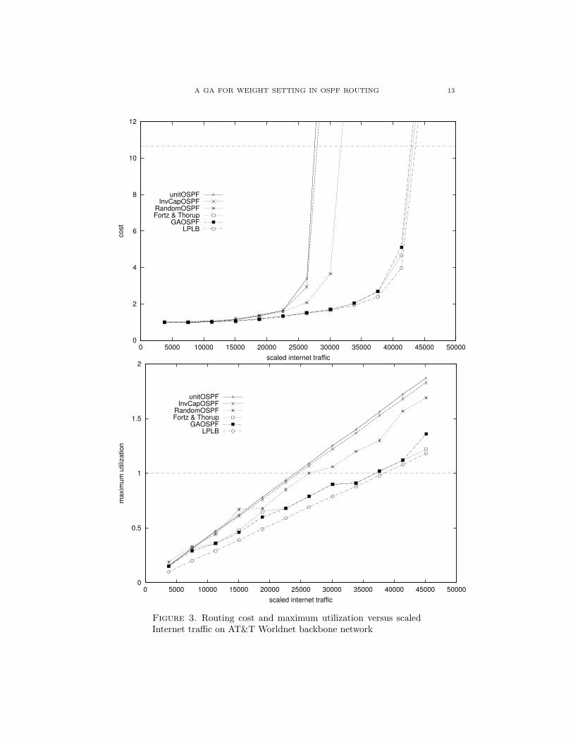
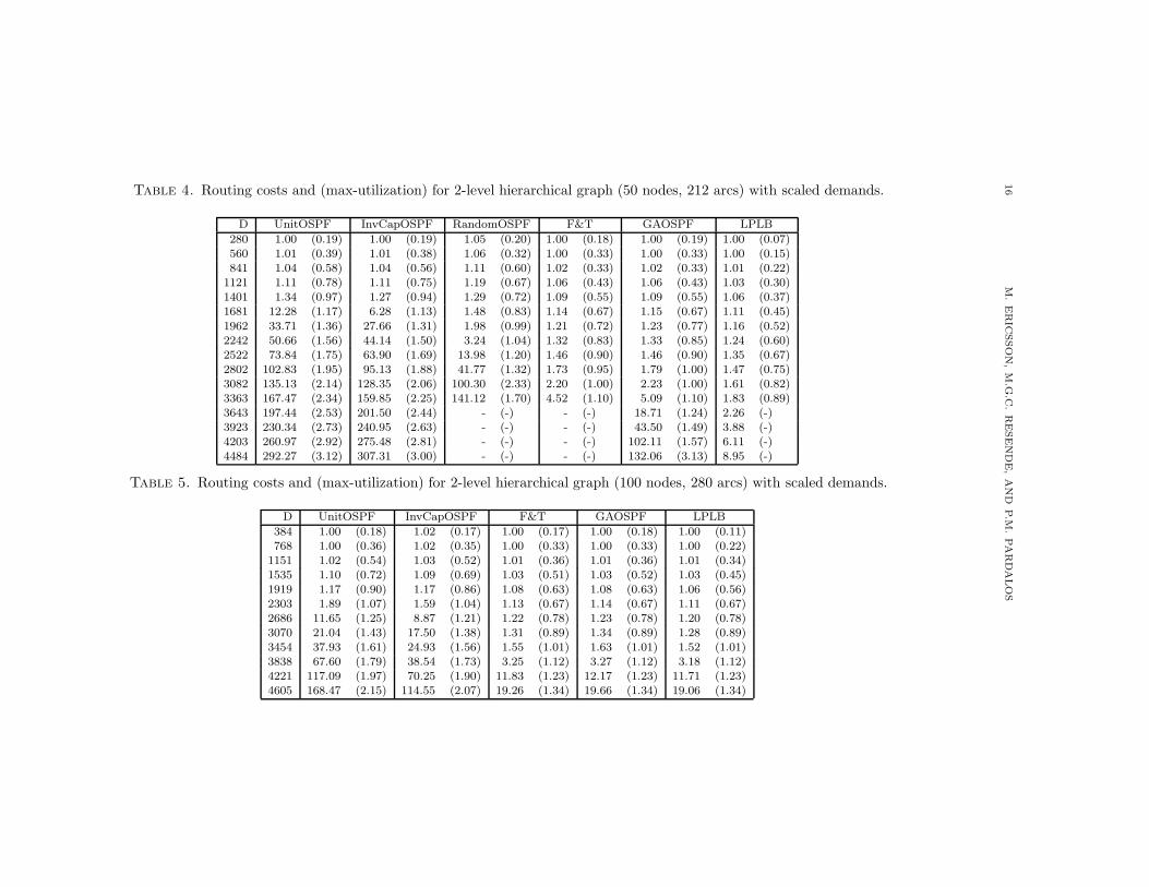
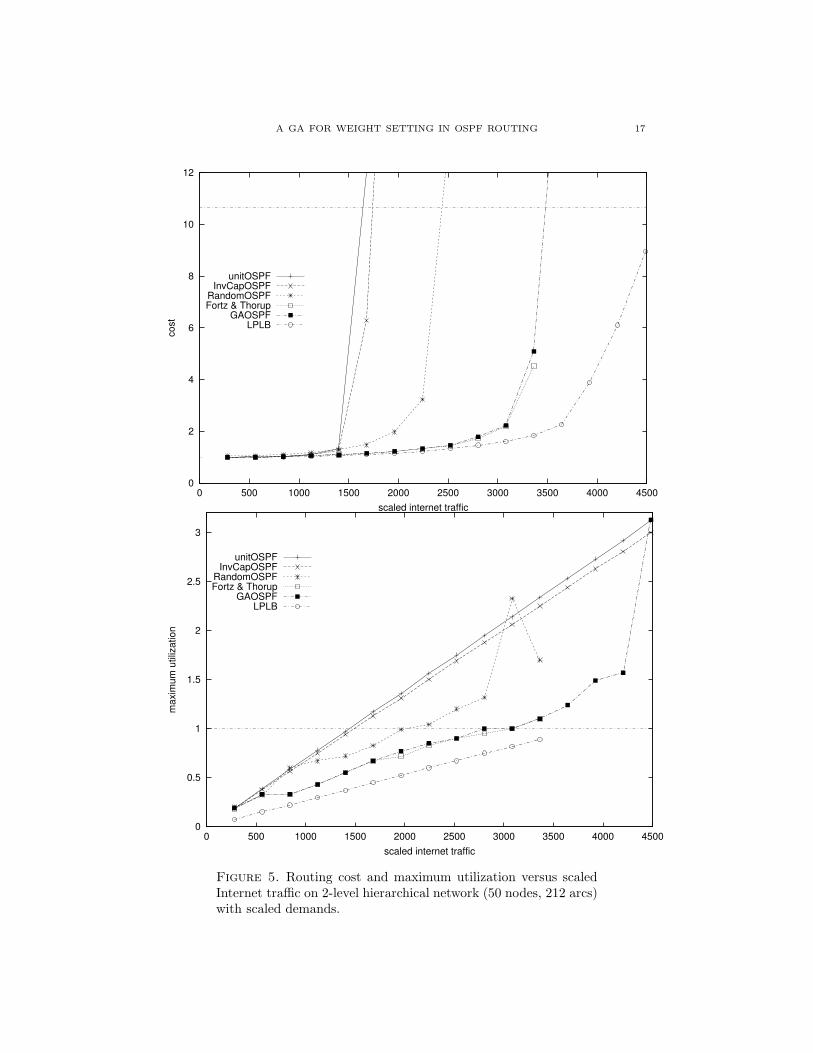
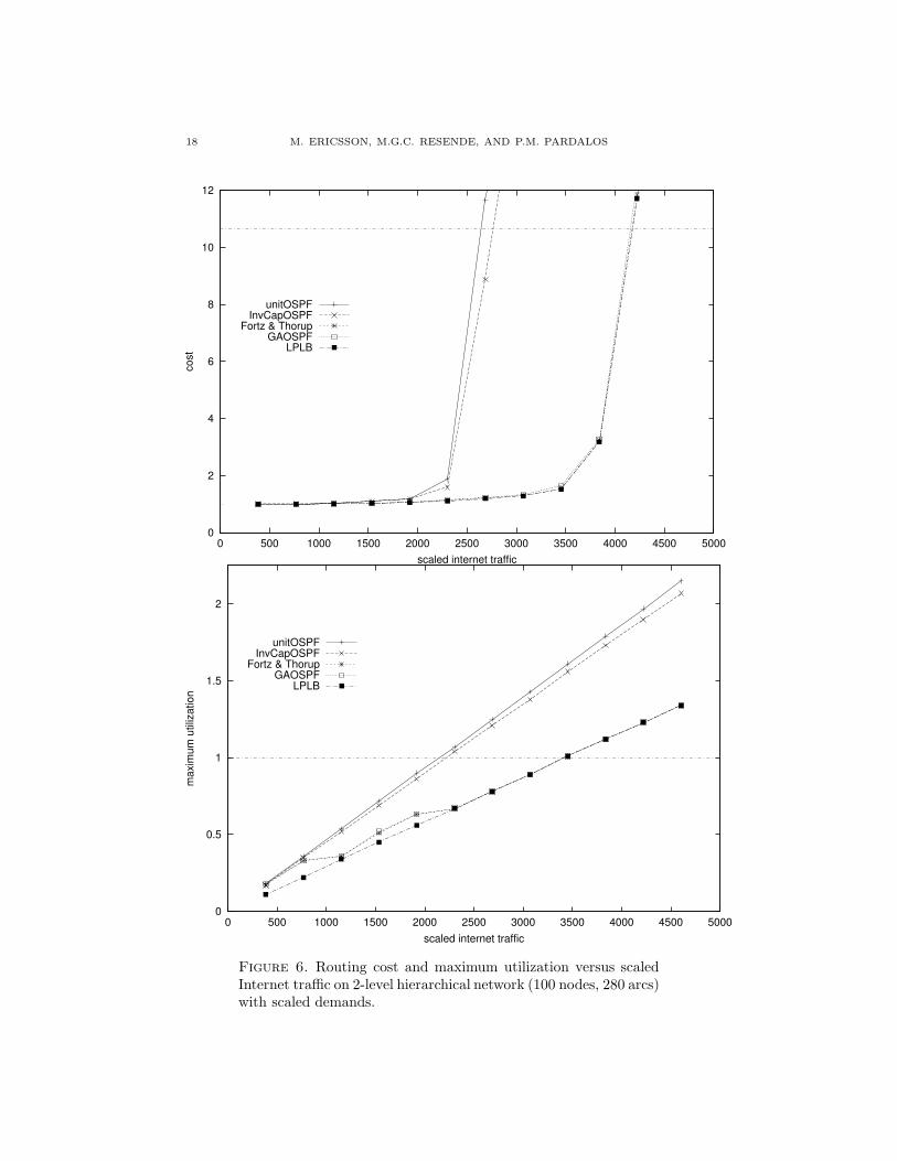
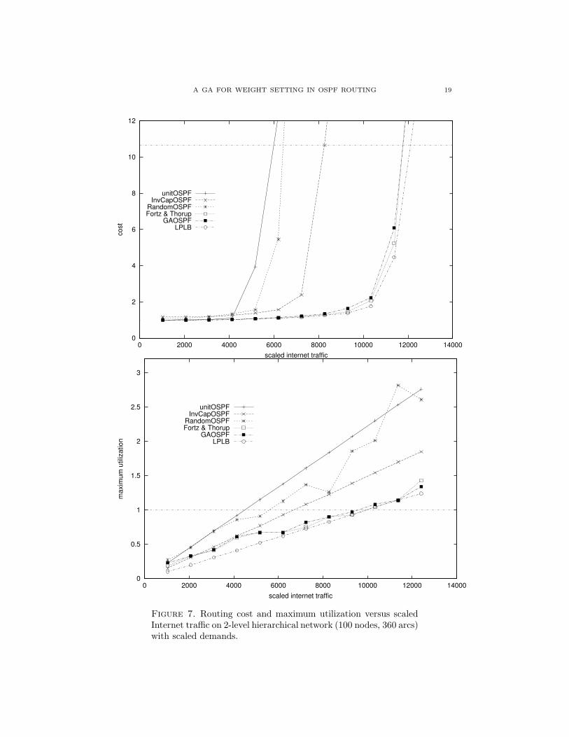
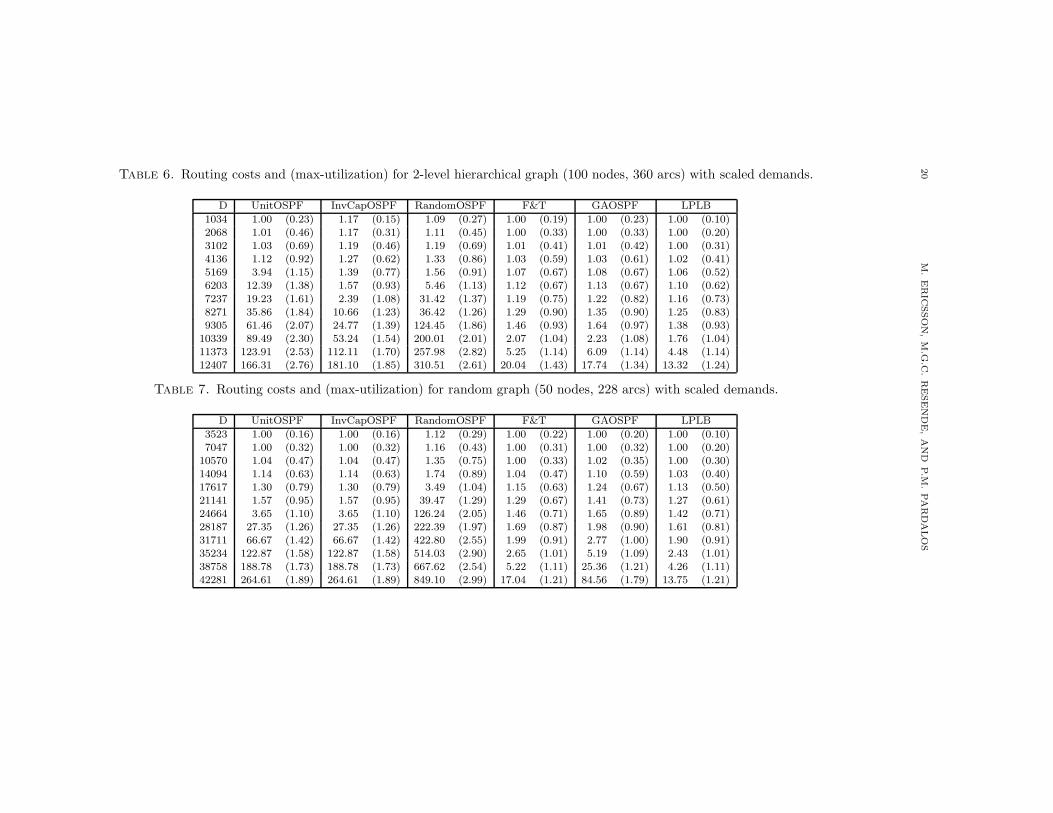
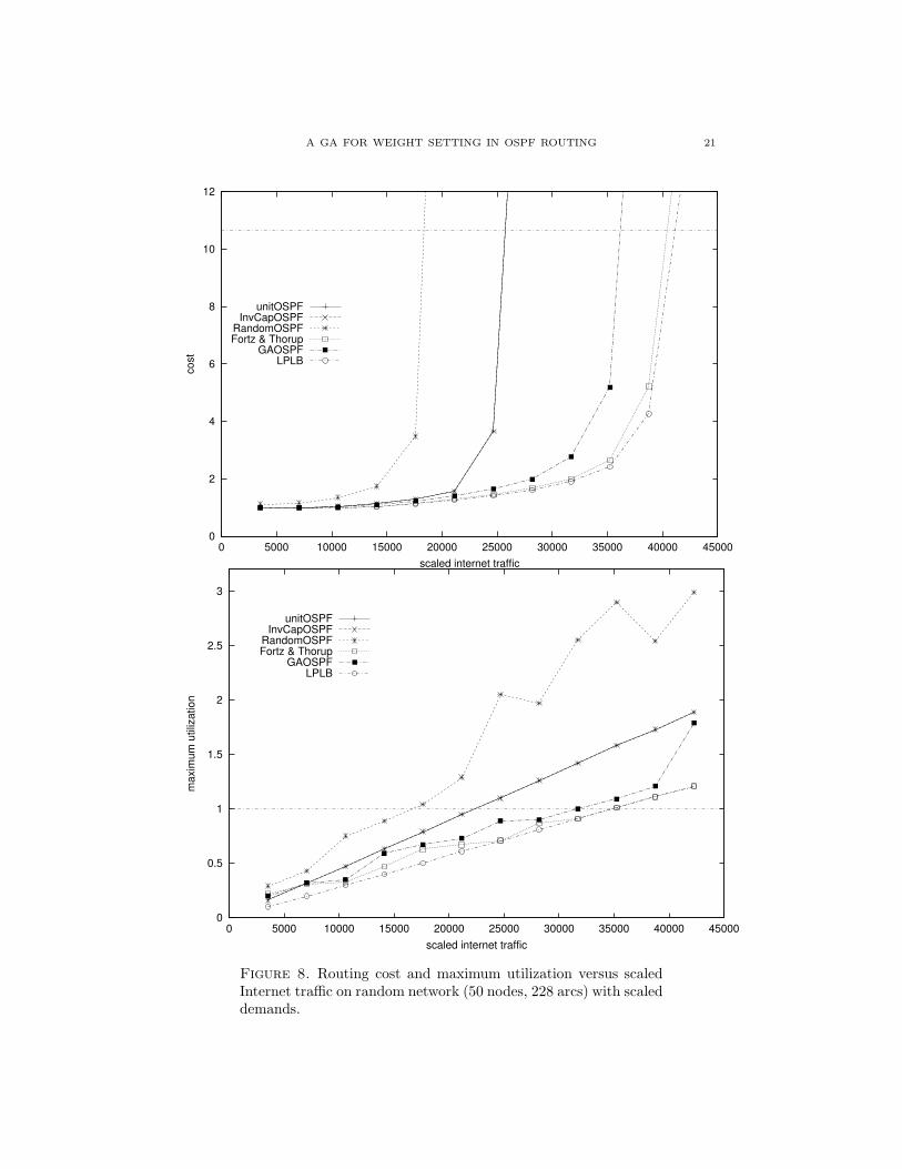
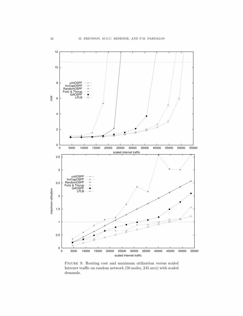
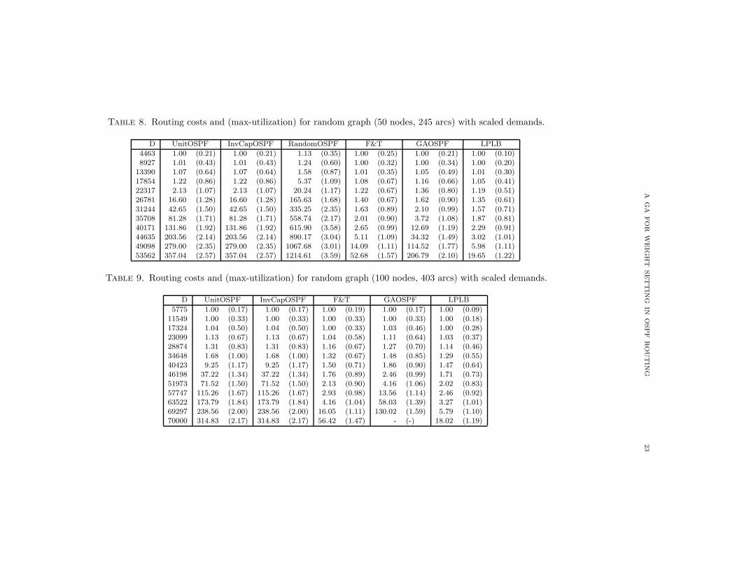
We next present the computational results for the thirteen test problems andthe five heuristics. For each test problem, we present one table and one figure withtwo plots. In the experiments, the heuristics and lower bounding procedure are runusing several levels of Internet traffic. This scaling of Internet traffic is done bysimply multiplying each entry in the demand matrix by a fixed number. We usethe scaling values used in [12].
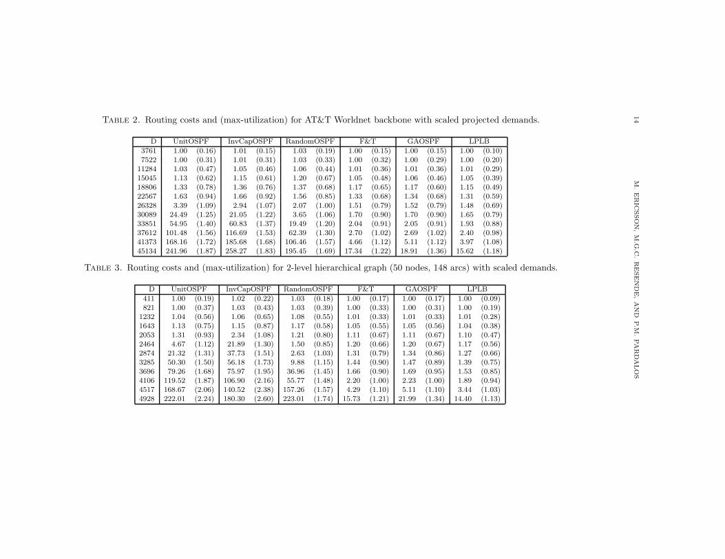
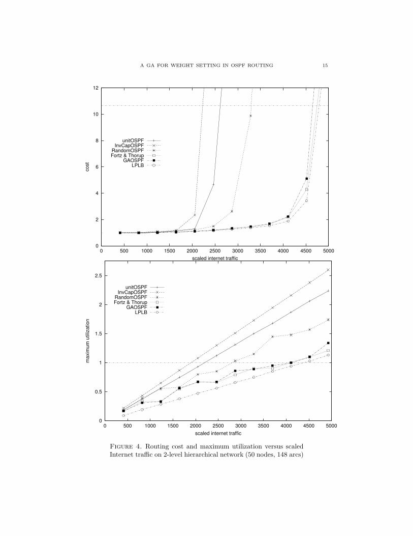
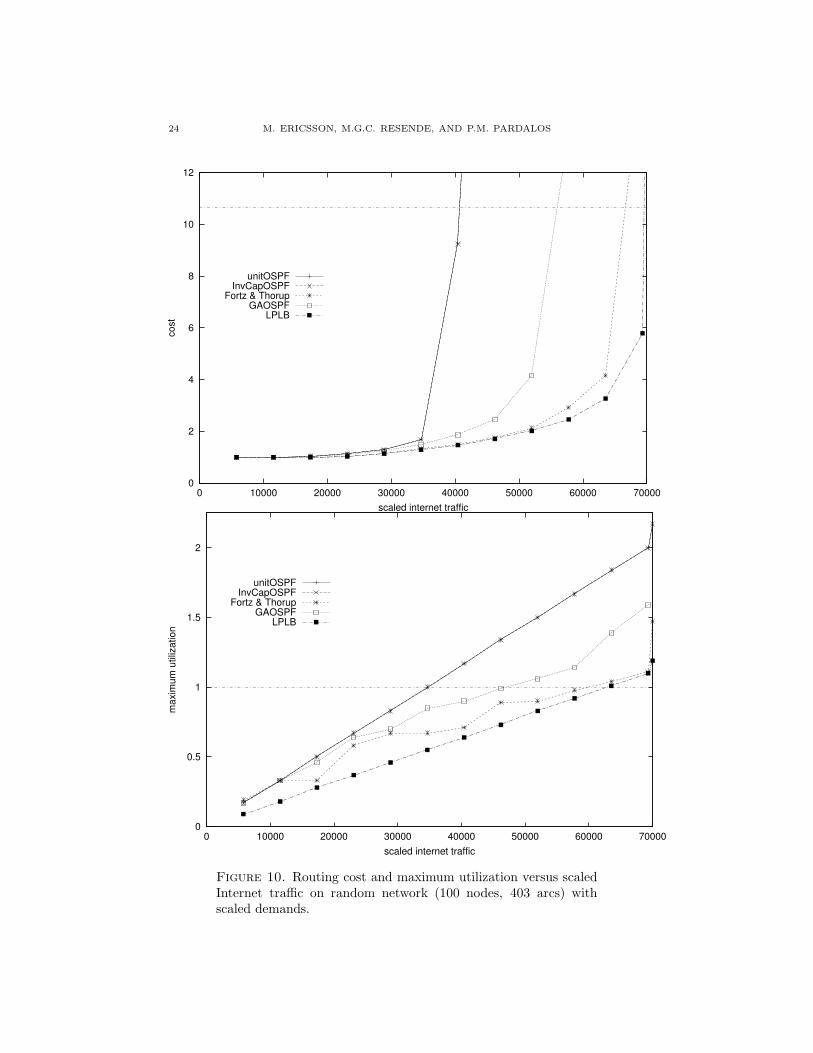
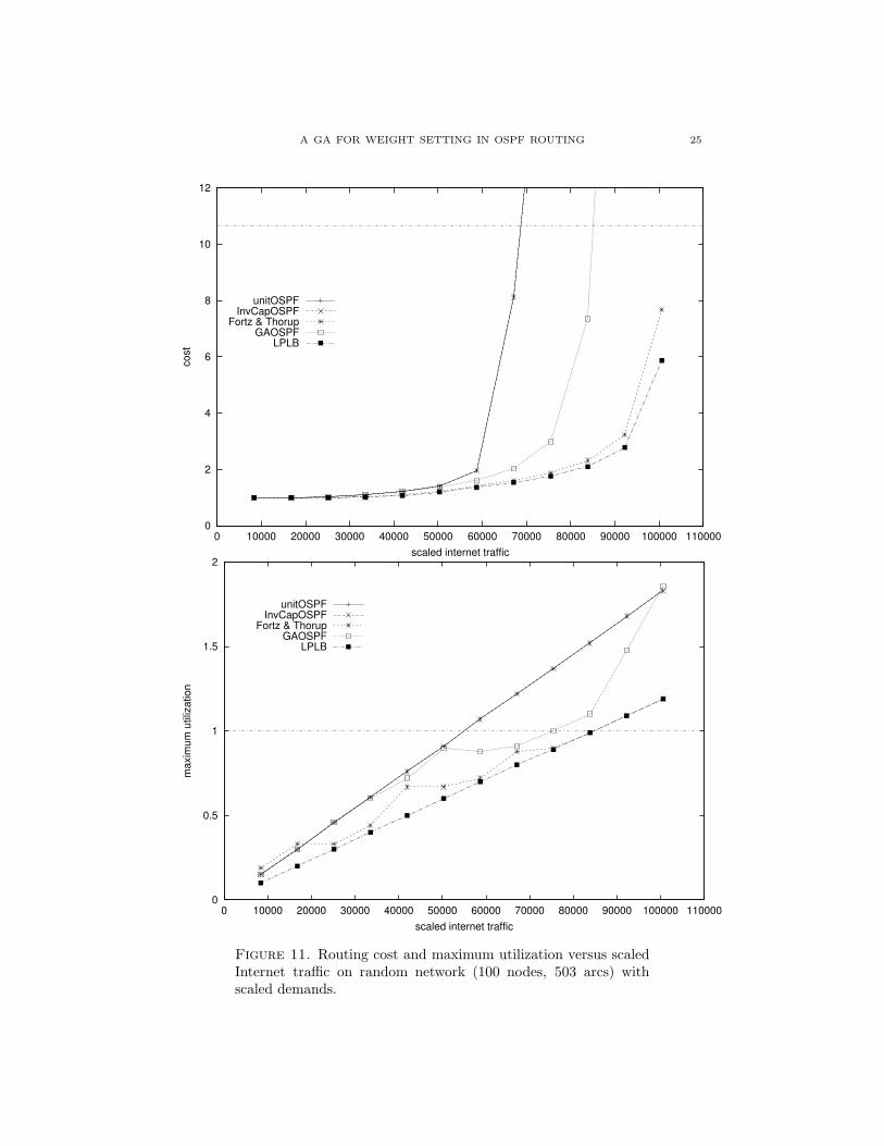
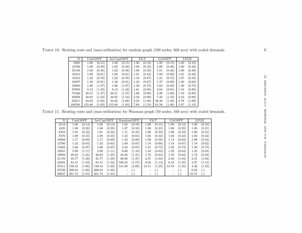
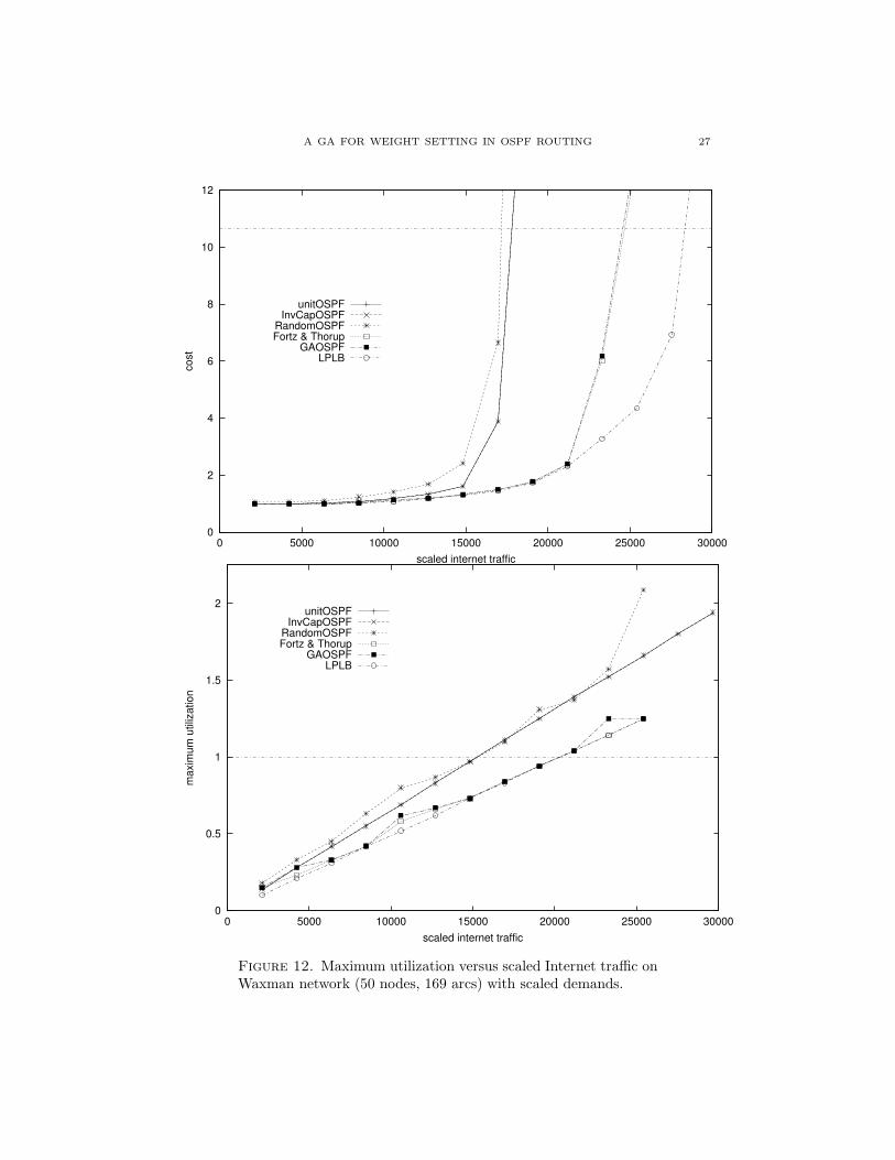
Table 2 and Figure 3 show the results for the AT&T Worldnet backbone networkinstance. Tables 3 – 6 and Figures 4 – 7 show the results for the 2-level hierarchicalnetwork instances. Tables 7 – 10 and Figures 8 – 11 show the results for the randomnetwork instances. Finally, Tables 11 – 14 and Figures 12 – 15 show the results forthe Waxman network instances. In the tables, we present the OSPF routing costsand the maximum utilizations for each of the heuristics and the LP lower bound, asa function of the total demand (D). The routing costs are normalized, as describedearlier, with the normalizing scaling factor Φuncap. In the routing cost figures,the dashed horizontal line corresponds to the threshold of 10.667, when networkcongestion is reached. By maximum utilization, we mean the arc utilization (totaltraffic on the arc load divided by arc capacity) of the maximum utilized arc in thenetwork. The maximum utilizations are listed in parenthesis in the tables.
We make the following remarks regarding the computational experiments. First,we observe that the GAOSPF generally finds good solutions close to the lowerbound. With the exception of the random networks, GAOSPF found solutionswith similar quality as those found by the Fortz and Thorup local search. Thesolutions found by GAOSPF were significantly better than those produced by Uni-tOSPF, InvCapOSPF, and RandomOSPF, and allowed a significant increase ofthe network’s throughput with respect to the throughputs associated with thoseheuristics.
GAOSPF works particularly well for the real-world AT&T Worldnet backboneinstance, where compared to the InvCapOSPF heuristic, it was able to increasenetwork traffic by 70% until the network becomes congested. Recall that InvCa-pOSPF is recommended by Cisco. GAOSPF also produces good solutions on theinstances of the 2-level hierarchical graphs and on the large Waxman graphs, wherethe gap to the lower bound is very small.
For the two instances of the 2-level hierarchical graphs with 50 nodes, GAOSPFproduced an average traffic increase of 105%, when compared with InvCapOSPF.The average traffic increase for all test problems was 52%.
Comparing the UnitOSPF and InvCapOSPF routing schemes, we see that In-vCapOSPF is slightly better than UnitOSPF for most instances. InvCapOSPF istherefore the most challenging of the simple heuristic to compete with.
A GA FOR WEIGHT SETTING IN OSPF ROUTING 13
0
2
4
6
8
10
12
0 5000 10000 15000 20000 25000 30000 35000 40000 45000 50000
cost
scaled internet traffic
unitOSPFInvCapOSPF
RandomOSPFFortz & Thorup
GAOSPFLPLB
0
0.5
1
1.5
2
0 5000 10000 15000 20000 25000 30000 35000 40000 45000 50000
max
imum
util
izat
ion
scaled internet traffic
unitOSPFInvCapOSPF
RandomOSPFFortz & Thorup
GAOSPFLPLB
Figure 3. Routing cost and maximum utilization versus scaledInternet traffic on AT&T Worldnet backbone network
14
M.
ER
ICSSO
N,
M.G
.C.
RE
SE
ND
E,
AN
DP
.M.
PA
RD
AL
OS
Table 2. Routing costs and (max-utilization) for AT&T Worldnet backbone with scaled projected demands.
D UnitOSPF InvCapOSPF RandomOSPF F&T GAOSPF LPLB
3761 1.00 (0.16) 1.01 (0.15) 1.03 (0.19) 1.00 (0.15) 1.00 (0.15) 1.00 (0.10)7522 1.00 (0.31) 1.01 (0.31) 1.03 (0.33) 1.00 (0.32) 1.00 (0.29) 1.00 (0.20)
11284 1.03 (0.47) 1.05 (0.46) 1.06 (0.44) 1.01 (0.36) 1.01 (0.36) 1.01 (0.29)15045 1.13 (0.62) 1.15 (0.61) 1.20 (0.67) 1.05 (0.48) 1.06 (0.46) 1.05 (0.39)18806 1.33 (0.78) 1.36 (0.76) 1.37 (0.68) 1.17 (0.65) 1.17 (0.60) 1.15 (0.49)22567 1.63 (0.94) 1.66 (0.92) 1.56 (0.85) 1.33 (0.68) 1.34 (0.68) 1.31 (0.59)
26328 3.39 (1.09) 2.94 (1.07) 2.07 (1.00) 1.51 (0.79) 1.52 (0.79) 1.48 (0.69)30089 24.49 (1.25) 21.05 (1.22) 3.65 (1.06) 1.70 (0.90) 1.70 (0.90) 1.65 (0.79)33851 54.95 (1.40) 60.83 (1.37) 19.49 (1.20) 2.04 (0.91) 2.05 (0.91) 1.93 (0.88)37612 101.48 (1.56) 116.69 (1.53) 62.39 (1.30) 2.70 (1.02) 2.69 (1.02) 2.40 (0.98)41373 168.16 (1.72) 185.68 (1.68) 106.46 (1.57) 4.66 (1.12) 5.11 (1.12) 3.97 (1.08)45134 241.96 (1.87) 258.27 (1.83) 195.45 (1.69) 17.34 (1.22) 18.91 (1.36) 15.62 (1.18)
Table 3. Routing costs and (max-utilization) for 2-level hierarchical graph (50 nodes, 148 arcs) with scaled demands.
D UnitOSPF InvCapOSPF RandomOSPF F&T GAOSPF LPLB
411 1.00 (0.19) 1.02 (0.22) 1.03 (0.18) 1.00 (0.17) 1.00 (0.17) 1.00 (0.09)821 1.00 (0.37) 1.03 (0.43) 1.03 (0.39) 1.00 (0.33) 1.00 (0.31) 1.00 (0.19)
1232 1.04 (0.56) 1.06 (0.65) 1.08 (0.55) 1.01 (0.33) 1.01 (0.33) 1.01 (0.28)1643 1.13 (0.75) 1.15 (0.87) 1.17 (0.58) 1.05 (0.55) 1.05 (0.56) 1.04 (0.38)2053 1.31 (0.93) 2.34 (1.08) 1.21 (0.80) 1.11 (0.67) 1.11 (0.67) 1.10 (0.47)2464 4.67 (1.12) 21.89 (1.30) 1.50 (0.85) 1.20 (0.66) 1.20 (0.67) 1.17 (0.56)2874 21.32 (1.31) 37.73 (1.51) 2.63 (1.03) 1.31 (0.79) 1.34 (0.86) 1.27 (0.66)3285 50.30 (1.50) 56.18 (1.73) 9.88 (1.15) 1.44 (0.90) 1.47 (0.89) 1.39 (0.75)3696 79.26 (1.68) 75.97 (1.95) 36.96 (1.45) 1.66 (0.90) 1.69 (0.95) 1.53 (0.85)4106 119.52 (1.87) 106.90 (2.16) 55.77 (1.48) 2.20 (1.00) 2.23 (1.00) 1.89 (0.94)4517 168.67 (2.06) 140.52 (2.38) 157.26 (1.57) 4.29 (1.10) 5.11 (1.10) 3.44 (1.03)4928 222.01 (2.24) 180.30 (2.60) 223.01 (1.74) 15.73 (1.21) 21.99 (1.34) 14.40 (1.13)
A GA FOR WEIGHT SETTING IN OSPF ROUTING 15
0
2
4
6
8
10
12
0 500 1000 1500 2000 2500 3000 3500 4000 4500 5000
cost
scaled internet traffic
unitOSPFInvCapOSPF
RandomOSPFFortz & Thorup
GAOSPFLPLB
0
0.5
1
1.5
2
2.5
0 500 1000 1500 2000 2500 3000 3500 4000 4500 5000
max
imum
util
izat
ion
scaled internet traffic
unitOSPFInvCapOSPF
RandomOSPFFortz & Thorup
GAOSPFLPLB
Figure 4. Routing cost and maximum utilization versus scaledInternet traffic on 2-level hierarchical network (50 nodes, 148 arcs)
16
M.
ER
ICSSO
N,
M.G
.C.
RE
SE
ND
E,
AN
DP
.M.
PA
RD
AL
OS
Table 4. Routing costs and (max-utilization) for 2-level hierarchical graph (50 nodes, 212 arcs) with scaled demands.
D UnitOSPF InvCapOSPF RandomOSPF F&T GAOSPF LPLB
280 1.00 (0.19) 1.00 (0.19) 1.05 (0.20) 1.00 (0.18) 1.00 (0.19) 1.00 (0.07)560 1.01 (0.39) 1.01 (0.38) 1.06 (0.32) 1.00 (0.33) 1.00 (0.33) 1.00 (0.15)841 1.04 (0.58) 1.04 (0.56) 1.11 (0.60) 1.02 (0.33) 1.02 (0.33) 1.01 (0.22)
1121 1.11 (0.78) 1.11 (0.75) 1.19 (0.67) 1.06 (0.43) 1.06 (0.43) 1.03 (0.30)1401 1.34 (0.97) 1.27 (0.94) 1.29 (0.72) 1.09 (0.55) 1.09 (0.55) 1.06 (0.37)1681 12.28 (1.17) 6.28 (1.13) 1.48 (0.83) 1.14 (0.67) 1.15 (0.67) 1.11 (0.45)
1962 33.71 (1.36) 27.66 (1.31) 1.98 (0.99) 1.21 (0.72) 1.23 (0.77) 1.16 (0.52)2242 50.66 (1.56) 44.14 (1.50) 3.24 (1.04) 1.32 (0.83) 1.33 (0.85) 1.24 (0.60)2522 73.84 (1.75) 63.90 (1.69) 13.98 (1.20) 1.46 (0.90) 1.46 (0.90) 1.35 (0.67)2802 102.83 (1.95) 95.13 (1.88) 41.77 (1.32) 1.73 (0.95) 1.79 (1.00) 1.47 (0.75)3082 135.13 (2.14) 128.35 (2.06) 100.30 (2.33) 2.20 (1.00) 2.23 (1.00) 1.61 (0.82)3363 167.47 (2.34) 159.85 (2.25) 141.12 (1.70) 4.52 (1.10) 5.09 (1.10) 1.83 (0.89)3643 197.44 (2.53) 201.50 (2.44) - (-) - (-) 18.71 (1.24) 2.26 (-)3923 230.34 (2.73) 240.95 (2.63) - (-) - (-) 43.50 (1.49) 3.88 (-)4203 260.97 (2.92) 275.48 (2.81) - (-) - (-) 102.11 (1.57) 6.11 (-)4484 292.27 (3.12) 307.31 (3.00) - (-) - (-) 132.06 (3.13) 8.95 (-)
Table 5. Routing costs and (max-utilization) for 2-level hierarchical graph (100 nodes, 280 arcs) with scaled demands.
D UnitOSPF InvCapOSPF F&T GAOSPF LPLB
384 1.00 (0.18) 1.02 (0.17) 1.00 (0.17) 1.00 (0.18) 1.00 (0.11)768 1.00 (0.36) 1.02 (0.35) 1.00 (0.33) 1.00 (0.33) 1.00 (0.22)
1151 1.02 (0.54) 1.03 (0.52) 1.01 (0.36) 1.01 (0.36) 1.01 (0.34)1535 1.10 (0.72) 1.09 (0.69) 1.03 (0.51) 1.03 (0.52) 1.03 (0.45)1919 1.17 (0.90) 1.17 (0.86) 1.08 (0.63) 1.08 (0.63) 1.06 (0.56)2303 1.89 (1.07) 1.59 (1.04) 1.13 (0.67) 1.14 (0.67) 1.11 (0.67)2686 11.65 (1.25) 8.87 (1.21) 1.22 (0.78) 1.23 (0.78) 1.20 (0.78)3070 21.04 (1.43) 17.50 (1.38) 1.31 (0.89) 1.34 (0.89) 1.28 (0.89)3454 37.93 (1.61) 24.93 (1.56) 1.55 (1.01) 1.63 (1.01) 1.52 (1.01)3838 67.60 (1.79) 38.54 (1.73) 3.25 (1.12) 3.27 (1.12) 3.18 (1.12)4221 117.09 (1.97) 70.25 (1.90) 11.83 (1.23) 12.17 (1.23) 11.71 (1.23)4605 168.47 (2.15) 114.55 (2.07) 19.26 (1.34) 19.66 (1.34) 19.06 (1.34)
A GA FOR WEIGHT SETTING IN OSPF ROUTING 17
0
2
4
6
8
10
12
0 500 1000 1500 2000 2500 3000 3500 4000 4500
cost
scaled internet traffic
unitOSPFInvCapOSPF
RandomOSPFFortz & Thorup
GAOSPFLPLB
0
0.5
1
1.5
2
2.5
3
0 500 1000 1500 2000 2500 3000 3500 4000 4500
max
imum
util
izat
ion
scaled internet traffic
unitOSPFInvCapOSPF
RandomOSPFFortz & Thorup
GAOSPFLPLB
Figure 5. Routing cost and maximum utilization versus scaledInternet traffic on 2-level hierarchical network (50 nodes, 212 arcs)with scaled demands.
18 M. ERICSSON, M.G.C. RESENDE, AND P.M. PARDALOS
0
2
4
6
8
10
12
0 500 1000 1500 2000 2500 3000 3500 4000 4500 5000
cost
scaled internet traffic
unitOSPFInvCapOSPF
Fortz & ThorupGAOSPF
LPLB
0
0.5
1
1.5
2
0 500 1000 1500 2000 2500 3000 3500 4000 4500 5000
max
imum
util
izat
ion
scaled internet traffic
unitOSPFInvCapOSPF
Fortz & ThorupGAOSPF
LPLB
Figure 6. Routing cost and maximum utilization versus scaledInternet traffic on 2-level hierarchical network (100 nodes, 280 arcs)with scaled demands.
A GA FOR WEIGHT SETTING IN OSPF ROUTING 19
0
2
4
6
8
10
12
0 2000 4000 6000 8000 10000 12000 14000
cost
scaled internet traffic
unitOSPFInvCapOSPF
RandomOSPFFortz & Thorup
GAOSPFLPLB
0
0.5
1
1.5
2
2.5
3
0 2000 4000 6000 8000 10000 12000 14000
max
imum
util
izat
ion
scaled internet traffic
unitOSPFInvCapOSPF
RandomOSPFFortz & Thorup
GAOSPFLPLB
Figure 7. Routing cost and maximum utilization versus scaledInternet traffic on 2-level hierarchical network (100 nodes, 360 arcs)with scaled demands.
20
M.
ER
ICSSO
N,
M.G
.C.
RE
SE
ND
E,
AN
DP
.M.
PA
RD
AL
OS
Table 6. Routing costs and (max-utilization) for 2-level hierarchical graph (100 nodes, 360 arcs) with scaled demands.
D UnitOSPF InvCapOSPF RandomOSPF F&T GAOSPF LPLB
1034 1.00 (0.23) 1.17 (0.15) 1.09 (0.27) 1.00 (0.19) 1.00 (0.23) 1.00 (0.10)2068 1.01 (0.46) 1.17 (0.31) 1.11 (0.45) 1.00 (0.33) 1.00 (0.33) 1.00 (0.20)3102 1.03 (0.69) 1.19 (0.46) 1.19 (0.69) 1.01 (0.41) 1.01 (0.42) 1.00 (0.31)4136 1.12 (0.92) 1.27 (0.62) 1.33 (0.86) 1.03 (0.59) 1.03 (0.61) 1.02 (0.41)5169 3.94 (1.15) 1.39 (0.77) 1.56 (0.91) 1.07 (0.67) 1.08 (0.67) 1.06 (0.52)6203 12.39 (1.38) 1.57 (0.93) 5.46 (1.13) 1.12 (0.67) 1.13 (0.67) 1.10 (0.62)
7237 19.23 (1.61) 2.39 (1.08) 31.42 (1.37) 1.19 (0.75) 1.22 (0.82) 1.16 (0.73)8271 35.86 (1.84) 10.66 (1.23) 36.42 (1.26) 1.29 (0.90) 1.35 (0.90) 1.25 (0.83)9305 61.46 (2.07) 24.77 (1.39) 124.45 (1.86) 1.46 (0.93) 1.64 (0.97) 1.38 (0.93)
10339 89.49 (2.30) 53.24 (1.54) 200.01 (2.01) 2.07 (1.04) 2.23 (1.08) 1.76 (1.04)11373 123.91 (2.53) 112.11 (1.70) 257.98 (2.82) 5.25 (1.14) 6.09 (1.14) 4.48 (1.14)12407 166.31 (2.76) 181.10 (1.85) 310.51 (2.61) 20.04 (1.43) 17.74 (1.34) 13.32 (1.24)
Table 7. Routing costs and (max-utilization) for random graph (50 nodes, 228 arcs) with scaled demands.
D UnitOSPF InvCapOSPF RandomOSPF F&T GAOSPF LPLB
3523 1.00 (0.16) 1.00 (0.16) 1.12 (0.29) 1.00 (0.22) 1.00 (0.20) 1.00 (0.10)7047 1.00 (0.32) 1.00 (0.32) 1.16 (0.43) 1.00 (0.31) 1.00 (0.32) 1.00 (0.20)
10570 1.04 (0.47) 1.04 (0.47) 1.35 (0.75) 1.00 (0.33) 1.02 (0.35) 1.00 (0.30)14094 1.14 (0.63) 1.14 (0.63) 1.74 (0.89) 1.04 (0.47) 1.10 (0.59) 1.03 (0.40)17617 1.30 (0.79) 1.30 (0.79) 3.49 (1.04) 1.15 (0.63) 1.24 (0.67) 1.13 (0.50)21141 1.57 (0.95) 1.57 (0.95) 39.47 (1.29) 1.29 (0.67) 1.41 (0.73) 1.27 (0.61)24664 3.65 (1.10) 3.65 (1.10) 126.24 (2.05) 1.46 (0.71) 1.65 (0.89) 1.42 (0.71)28187 27.35 (1.26) 27.35 (1.26) 222.39 (1.97) 1.69 (0.87) 1.98 (0.90) 1.61 (0.81)31711 66.67 (1.42) 66.67 (1.42) 422.80 (2.55) 1.99 (0.91) 2.77 (1.00) 1.90 (0.91)35234 122.87 (1.58) 122.87 (1.58) 514.03 (2.90) 2.65 (1.01) 5.19 (1.09) 2.43 (1.01)38758 188.78 (1.73) 188.78 (1.73) 667.62 (2.54) 5.22 (1.11) 25.36 (1.21) 4.26 (1.11)42281 264.61 (1.89) 264.61 (1.89) 849.10 (2.99) 17.04 (1.21) 84.56 (1.79) 13.75 (1.21)
A GA FOR WEIGHT SETTING IN OSPF ROUTING 21
0
2
4
6
8
10
12
0 5000 10000 15000 20000 25000 30000 35000 40000 45000
cost
scaled internet traffic
unitOSPFInvCapOSPF
RandomOSPFFortz & Thorup
GAOSPFLPLB
0
0.5
1
1.5
2
2.5
3
0 5000 10000 15000 20000 25000 30000 35000 40000 45000
max
imum
util
izat
ion
scaled internet traffic
unitOSPFInvCapOSPF
RandomOSPFFortz & Thorup
GAOSPFLPLB
Figure 8. Routing cost and maximum utilization versus scaledInternet traffic on random network (50 nodes, 228 arcs) with scaleddemands.
22 M. ERICSSON, M.G.C. RESENDE, AND P.M. PARDALOS
0
2
4
6
8
10
12
0 5000 10000 15000 20000 25000 30000 35000 40000 45000 50000 55000
cost
scaled internet traffic
unitOSPFInvCapOSPF
RandomOSPFFortz & Thorup
GAOSPFLPLB
0
0.5
1
1.5
2
2.5
3
3.5
0 5000 10000 15000 20000 25000 30000 35000 40000 45000 50000 55000
max
imum
util
izat
ion
scaled internet traffic
unitOSPFInvCapOSPF
RandomOSPFFortz & Thorup
GAOSPFLPLB
Figure 9. Routing cost and maximum utilization versus scaledInternet traffic on random network (50 nodes, 245 arcs) with scaleddemands.
AG
AF
OR
WE
IGH
TSE
TT
ING
INO
SP
FR
OU
TIN
G23
Table 8. Routing costs and (max-utilization) for random graph (50 nodes, 245 arcs) with scaled demands.
D UnitOSPF InvCapOSPF RandomOSPF F&T GAOSPF LPLB
4463 1.00 (0.21) 1.00 (0.21) 1.13 (0.35) 1.00 (0.25) 1.00 (0.21) 1.00 (0.10)8927 1.01 (0.43) 1.01 (0.43) 1.24 (0.60) 1.00 (0.32) 1.00 (0.34) 1.00 (0.20)
13390 1.07 (0.64) 1.07 (0.64) 1.58 (0.87) 1.01 (0.35) 1.05 (0.49) 1.01 (0.30)17854 1.22 (0.86) 1.22 (0.86) 5.37 (1.09) 1.08 (0.67) 1.16 (0.66) 1.05 (0.41)22317 2.13 (1.07) 2.13 (1.07) 20.24 (1.17) 1.22 (0.67) 1.36 (0.80) 1.19 (0.51)26781 16.60 (1.28) 16.60 (1.28) 165.63 (1.68) 1.40 (0.67) 1.62 (0.90) 1.35 (0.61)
31244 42.65 (1.50) 42.65 (1.50) 335.25 (2.35) 1.63 (0.89) 2.10 (0.99) 1.57 (0.71)35708 81.28 (1.71) 81.28 (1.71) 558.74 (2.17) 2.01 (0.90) 3.72 (1.08) 1.87 (0.81)40171 131.86 (1.92) 131.86 (1.92) 615.90 (3.58) 2.65 (0.99) 12.69 (1.19) 2.29 (0.91)44635 203.56 (2.14) 203.56 (2.14) 890.17 (3.04) 5.11 (1.09) 34.32 (1.49) 3.02 (1.01)49098 279.00 (2.35) 279.00 (2.35) 1067.68 (3.01) 14.09 (1.11) 114.52 (1.77) 5.98 (1.11)53562 357.04 (2.57) 357.04 (2.57) 1214.61 (3.59) 52.68 (1.57) 206.79 (2.10) 19.65 (1.22)
Table 9. Routing costs and (max-utilization) for random graph (100 nodes, 403 arcs) with scaled demands.
D UnitOSPF InvCapOSPF F&T GAOSPF LPLB
5775 1.00 (0.17) 1.00 (0.17) 1.00 (0.19) 1.00 (0.17) 1.00 (0.09)11549 1.00 (0.33) 1.00 (0.33) 1.00 (0.33) 1.00 (0.33) 1.00 (0.18)17324 1.04 (0.50) 1.04 (0.50) 1.00 (0.33) 1.03 (0.46) 1.00 (0.28)23099 1.13 (0.67) 1.13 (0.67) 1.04 (0.58) 1.11 (0.64) 1.03 (0.37)28874 1.31 (0.83) 1.31 (0.83) 1.16 (0.67) 1.27 (0.70) 1.14 (0.46)34648 1.68 (1.00) 1.68 (1.00) 1.32 (0.67) 1.48 (0.85) 1.29 (0.55)40423 9.25 (1.17) 9.25 (1.17) 1.50 (0.71) 1.86 (0.90) 1.47 (0.64)46198 37.22 (1.34) 37.22 (1.34) 1.76 (0.89) 2.46 (0.99) 1.71 (0.73)51973 71.52 (1.50) 71.52 (1.50) 2.13 (0.90) 4.16 (1.06) 2.02 (0.83)57747 115.26 (1.67) 115.26 (1.67) 2.93 (0.98) 13.56 (1.14) 2.46 (0.92)63522 173.79 (1.84) 173.79 (1.84) 4.16 (1.04) 58.03 (1.39) 3.27 (1.01)69297 238.56 (2.00) 238.56 (2.00) 16.05 (1.11) 130.02 (1.59) 5.79 (1.10)70000 314.83 (2.17) 314.83 (2.17) 56.42 (1.47) - (-) 18.02 (1.19)
24 M. ERICSSON, M.G.C. RESENDE, AND P.M. PARDALOS
0
2
4
6
8
10
12
0 10000 20000 30000 40000 50000 60000 70000
cost
scaled internet traffic
unitOSPFInvCapOSPF
Fortz & ThorupGAOSPF
LPLB
0
0.5
1
1.5
2
0 10000 20000 30000 40000 50000 60000 70000
max
imum
util
izat
ion
scaled internet traffic
unitOSPFInvCapOSPF
Fortz & ThorupGAOSPF
LPLB
Figure 10. Routing cost and maximum utilization versus scaledInternet traffic on random network (100 nodes, 403 arcs) withscaled demands.
A GA FOR WEIGHT SETTING IN OSPF ROUTING 25
0
2
4
6
8
10
12
0 10000 20000 30000 40000 50000 60000 70000 80000 90000 100000 110000
cost
scaled internet traffic
unitOSPFInvCapOSPF
Fortz & ThorupGAOSPF
LPLB
0
0.5
1
1.5
2
0 10000 20000 30000 40000 50000 60000 70000 80000 90000 100000 110000
max
imum
util
izat
ion
scaled internet traffic
unitOSPFInvCapOSPF
Fortz & ThorupGAOSPF
LPLB
Figure 11. Routing cost and maximum utilization versus scaledInternet traffic on random network (100 nodes, 503 arcs) withscaled demands.
26
M.
ER
ICSSO
N,
M.G
.C.
RE
SE
ND
E,
AN
DP
.M.
PA
RD
AL
OS
Table 10. Routing costs and (max-utilization) for random graph (100 nodes, 503 arcs) with scaled demands.
D UnitOSPF InvCapOSPF F&T GAOSPF LPLB
8383 1.00 (0.15) 1.00 (0.15) 1.00 (0.19) 1.00 (0.15) 1.00 (0.10)16766 1.00 (0.30) 1.00 (0.30) 1.00 (0.33) 1.00 (0.30) 1.00 (0.20)25149 1.02 (0.46) 1.02 (0.46) 1.00 (0.33) 1.01 (0.46) 1.00 (0.30)33531 1.09 (0.61) 1.09 (0.61) 1.01 (0.44) 1.09 (0.60) 1.01 (0.40)41914 1.22 (0.76) 1.22 (0.76) 1.10 (0.67) 1.21 (0.72) 1.07 (0.50)50297 1.40 (0.91) 1.40 (0.91) 1.23 (0.67) 1.37 (0.90) 1.20 (0.60)
58680 1.96 (1.07) 1.96 (1.07) 1.40 (0.72) 1.62 (0.88) 1.36 (0.70)67063 8.13 (1.22) 8.13 (1.22) 1.61 (0.88) 2.04 (0.91) 1.54 (0.80)75446 20.51 (1.37) 20.51 (1.37) 1.86 (0.90) 2.98 (1.00) 1.76 (0.89)83829 48.85 (1.52) 48.85 (1.52) 2.32 (0.99) 7.35 (1.10) 2.10 (0.99)92211 94.05 (1.68) 94.05 (1.68) 3.23 (1.09) 30.40 (1.48) 2.78 (1.09)
100594 155.68 (1.83) 155.68 (1.83) 7.68 (1.19) 81.50 (1.86) 5.87 (1.19)
Table 11. Routing costs and (max-utilization) for Waxman graph (50 nodes, 169 arcs) with scaled demands.
D UnitOSPF InvCapOSPF RandomOSPF F&T GAOSPF LPLB
2118 1.00 (0.14) 1.00 (0.14) 1.05 (0.18) 1.00 (0.15) 1.00 (0.15) 1.00 (0.10)4235 1.00 (0.28) 1.00 (0.28) 1.07 (0.33) 1.00 (0.23) 1.00 (0.28) 1.00 (0.21)6353 1.01 (0.42) 1.01 (0.42) 1.11 (0.45) 1.00 (0.33) 1.00 (0.33) 1.00 (0.31)8470 1.08 (0.55) 1.08 (0.55) 1.24 (0.63) 1.02 (0.42) 1.02 (0.42) 1.02 (0.42)
10588 1.17 (0.69) 1.17 (0.69) 1.42 (0.80) 1.09 (0.58) 1.14 (0.62) 1.08 (0.52)12706 1.32 (0.83) 1.32 (0.83) 1.69 (0.87) 1.18 (0.66) 1.19 (0.67) 1.18 (0.62)14823 1.60 (0.97) 1.60 (0.97) 2.42 (0.97) 1.31 (0.73) 1.32 (0.73) 1.29 (0.73)16941 3.90 (1.11) 3.90 (1.11) 6.66 (1.10) 1.48 (0.84) 1.50 (0.84) 1.45 (0.83)19059 20.63 (1.25) 20.63 (1.25) 45.92 (1.31) 1.76 (0.94) 1.78 (0.94) 1.72 (0.94)21176 45.77 (1.39) 45.77 (1.39) 98.08 (1.37) 2.37 (1.04) 2.40 (1.04) 2.31 (1.04)23294 84.41 (1.52) 84.41 (1.52) 198.25 (1.57) 6.02 (1.14) 6.18 (1.25) 3.27 (1.14)25411 139.52 (1.66) 139.52 (1.66) 314.38 (2.09) 13.15 (1.25) 13.79 (1.25) 4.36 (1.25)27529 200.04 (1.80) 200.04 (1.80) - (-) - (-) - (-) 6.93 (-)29647 261.73 (1.94) 261.73 (1.94) - (-) - (-) - (-) 16.75 (-)
A GA FOR WEIGHT SETTING IN OSPF ROUTING 27
0
2
4
6
8
10
12
0 5000 10000 15000 20000 25000 30000
cost
scaled internet traffic
unitOSPFInvCapOSPF
RandomOSPFFortz & Thorup
GAOSPFLPLB
0
0.5
1
1.5
2
0 5000 10000 15000 20000 25000 30000
max
imum
util
izat
ion
scaled internet traffic
unitOSPFInvCapOSPF
RandomOSPFFortz & Thorup
GAOSPFLPLB
Figure 12. Maximum utilization versus scaled Internet traffic onWaxman network (50 nodes, 169 arcs) with scaled demands.
28 M. ERICSSON, M.G.C. RESENDE, AND P.M. PARDALOS
0
2
4
6
8
10
12
0 5000 10000 15000 20000 25000 30000 35000 40000 45000 50000
cost
scaled internet traffic
unitOSPFInvCapOSPF
RandomOSPFFortz & Thorup
GAOSPFLPLB
0
0.5
1
1.5
2
2.5
0 5000 10000 15000 20000 25000 30000 35000 40000 45000 50000
max
imum
util
izat
ion
scaled internet traffic
unitOSPFInvCapOSPF
RandomOSPFFortz & Thorup
GAOSPFLPLB
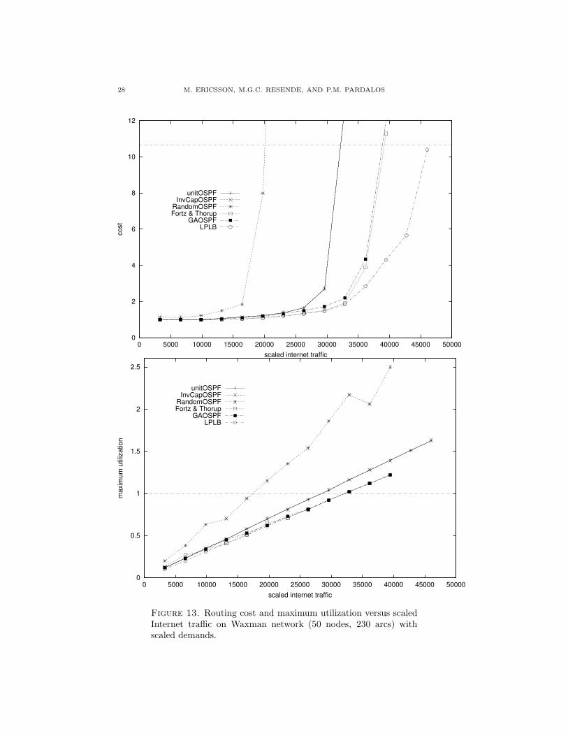
Figure 13. Routing cost and maximum utilization versus scaledInternet traffic on Waxman network (50 nodes, 230 arcs) withscaled demands.
AG
AF
OR
WE
IGH
TSE
TT
ING
INO
SP
FR
OU
TIN
G29
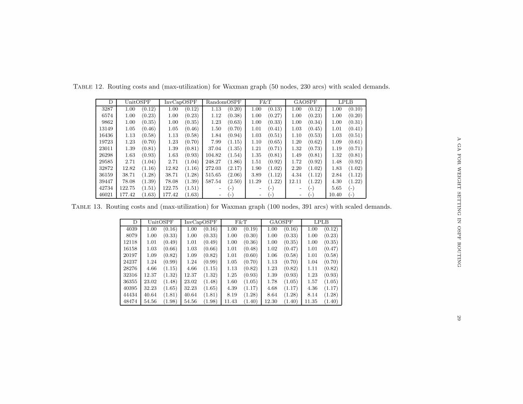
Table 12. Routing costs and (max-utilization) for Waxman graph (50 nodes, 230 arcs) with scaled demands.
D UnitOSPF InvCapOSPF RandomOSPF F&T GAOSPF LPLB
3287 1.00 (0.12) 1.00 (0.12) 1.13 (0.20) 1.00 (0.13) 1.00 (0.12) 1.00 (0.10)6574 1.00 (0.23) 1.00 (0.23) 1.12 (0.38) 1.00 (0.27) 1.00 (0.23) 1.00 (0.20)9862 1.00 (0.35) 1.00 (0.35) 1.23 (0.63) 1.00 (0.33) 1.00 (0.34) 1.00 (0.31)
13149 1.05 (0.46) 1.05 (0.46) 1.50 (0.70) 1.01 (0.41) 1.03 (0.45) 1.01 (0.41)16436 1.13 (0.58) 1.13 (0.58) 1.84 (0.94) 1.03 (0.51) 1.10 (0.53) 1.03 (0.51)19723 1.23 (0.70) 1.23 (0.70) 7.99 (1.15) 1.10 (0.65) 1.20 (0.62) 1.09 (0.61)
23011 1.39 (0.81) 1.39 (0.81) 37.04 (1.35) 1.21 (0.71) 1.32 (0.73) 1.19 (0.71)26298 1.63 (0.93) 1.63 (0.93) 104.82 (1.54) 1.35 (0.81) 1.49 (0.81) 1.32 (0.81)29585 2.71 (1.04) 2.71 (1.04) 248.27 (1.86) 1.51 (0.92) 1.72 (0.92) 1.48 (0.92)32872 12.82 (1.16) 12.82 (1.16) 272.03 (2.17) 1.90 (1.02) 2.20 (1.02) 1.83 (1.02)36159 38.71 (1.28) 38.71 (1.28) 515.65 (2.06) 3.89 (1.12) 4.34 (1.12) 2.84 (1.12)39447 78.08 (1.39) 78.08 (1.39) 587.54 (2.50) 11.29 (1.22) 12.11 (1.22) 4.30 (1.22)42734 122.75 (1.51) 122.75 (1.51) - (-) - (-) - (-) 5.65 (-)46021 177.42 (1.63) 177.42 (1.63) - (-) - (-) - (-) 10.40 (-)
Table 13. Routing costs and (max-utilization) for Waxman graph (100 nodes, 391 arcs) with scaled demands.
D UnitOSPF InvCapOSPF F&T GAOSPF LPLB
4039 1.00 (0.16) 1.00 (0.16) 1.00 (0.19) 1.00 (0.16) 1.00 (0.12)8079 1.00 (0.33) 1.00 (0.33) 1.00 (0.30) 1.00 (0.33) 1.00 (0.23)
12118 1.01 (0.49) 1.01 (0.49) 1.00 (0.36) 1.00 (0.35) 1.00 (0.35)16158 1.03 (0.66) 1.03 (0.66) 1.01 (0.48) 1.02 (0.47) 1.01 (0.47)20197 1.09 (0.82) 1.09 (0.82) 1.01 (0.60) 1.06 (0.58) 1.01 (0.58)24237 1.24 (0.99) 1.24 (0.99) 1.05 (0.70) 1.13 (0.70) 1.04 (0.70)28276 4.66 (1.15) 4.66 (1.15) 1.13 (0.82) 1.23 (0.82) 1.11 (0.82)32316 12.37 (1.32) 12.37 (1.32) 1.25 (0.93) 1.39 (0.93) 1.23 (0.93)36355 23.02 (1.48) 23.02 (1.48) 1.60 (1.05) 1.78 (1.05) 1.57 (1.05)40395 32.23 (1.65) 32.23 (1.65) 4.39 (1.17) 4.68 (1.17) 4.36 (1.17)44434 40.64 (1.81) 40.64 (1.81) 8.19 (1.28) 8.64 (1.28) 8.14 (1.28)48474 54.56 (1.98) 54.56 (1.98) 11.43 (1.40) 12.30 (1.40) 11.35 (1.40)
30 M. ERICSSON, M.G.C. RESENDE, AND P.M. PARDALOS
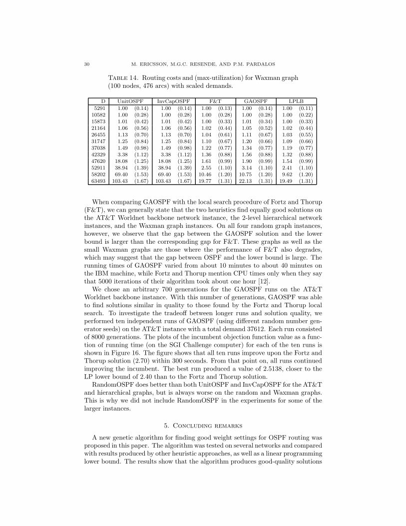
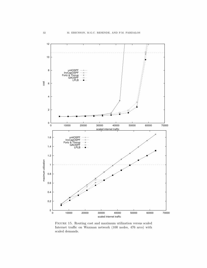
Table 14. Routing costs and (max-utilization) for Waxman graph(100 nodes, 476 arcs) with scaled demands.
D UnitOSPF InvCapOSPF F&T GAOSPF LPLB
5291 1.00 (0.14) 1.00 (0.14) 1.00 (0.13) 1.00 (0.14) 1.00 (0.11)10582 1.00 (0.28) 1.00 (0.28) 1.00 (0.28) 1.00 (0.28) 1.00 (0.22)15873 1.01 (0.42) 1.01 (0.42) 1.00 (0.33) 1.01 (0.34) 1.00 (0.33)21164 1.06 (0.56) 1.06 (0.56) 1.02 (0.44) 1.05 (0.52) 1.02 (0.44)26455 1.13 (0.70) 1.13 (0.70) 1.04 (0.61) 1.11 (0.67) 1.03 (0.55)31747 1.25 (0.84) 1.25 (0.84) 1.10 (0.67) 1.20 (0.66) 1.09 (0.66)37038 1.49 (0.98) 1.49 (0.98) 1.22 (0.77) 1.34 (0.77) 1.19 (0.77)42329 3.38 (1.12) 3.38 (1.12) 1.36 (0.88) 1.56 (0.88) 1.32 (0.88)47620 18.08 (1.25) 18.08 (1.25) 1.61 (0.99) 1.90 (0.99) 1.54 (0.99)52911 38.94 (1.39) 38.94 (1.39) 2.55 (1.10) 3.14 (1.10) 2.41 (1.10)58202 69.40 (1.53) 69.40 (1.53) 10.46 (1.20) 10.75 (1.20) 9.62 (1.20)63493 103.43 (1.67) 103.43 (1.67) 19.77 (1.31) 22.13 (1.31) 19.49 (1.31)
When comparing GAOSPF with the local search procedure of Fortz and Thorup(F&T), we can generally state that the two heuristics find equally good solutions onthe AT&T Worldnet backbone network instance, the 2-level hierarchical networkinstances, and the Waxman graph instances. On all four random graph instances,however, we observe that the gap between the GAOSPF solution and the lowerbound is larger than the corresponding gap for F&T. These graphs as well as thesmall Waxman graphs are those where the performance of F&T also degrades,which may suggest that the gap between OSPF and the lower bound is large. Therunning times of GAOSPF varied from about 10 minutes to about 40 minutes onthe IBM machine, while Fortz and Thorup mention CPU times only when they saythat 5000 iterations of their algorithm took about one hour [12].
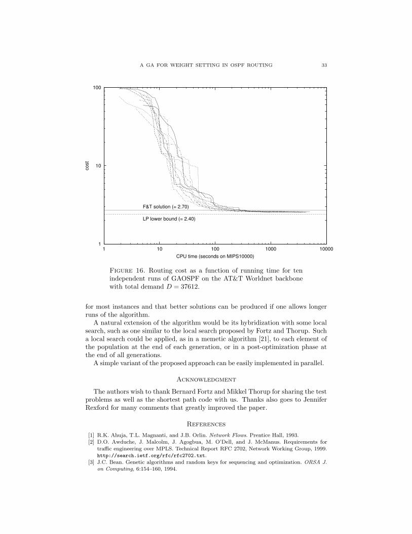
We chose an arbitrary 700 generations for the GAOSPF runs on the AT&TWorldnet backbone instance. With this number of generations, GAOSPF was ableto find solutions similar in quality to those found by the Fortz and Thorup localsearch. To investigate the tradeoff between longer runs and solution quality, weperformed ten independent runs of GAOSPF (using different random number gen-erator seeds) on the AT&T instance with a total demand 37612. Each run consistedof 8000 generations. The plots of the incumbent objection function value as a func-tion of running time (on the SGI Challenge computer) for each of the ten runs isshown in Figure 16. The figure shows that all ten runs improve upon the Fortz andThorup solution (2.70) within 300 seconds. From that point on, all runs continuedimproving the incumbent. The best run produced a value of 2.5138, closer to theLP lower bound of 2.40 than to the Fortz and Thorup solution.
RandomOSPF does better than both UnitOSPF and InvCapOSPF for the AT&Tand hierarchical graphs, but is always worse on the random and Waxman graphs.This is why we did not include RandomOSPF in the experiments for some of thelarger instances.
5. Concluding remarks
A new genetic algorithm for finding good weight settings for OSPF routing wasproposed in this paper. The algorithm was tested on several networks and comparedwith results produced by other heuristic approaches, as well as a linear programminglower bound. The results show that the algorithm produces good-quality solutions
A GA FOR WEIGHT SETTING IN OSPF ROUTING 31
0
2
4
6
8
10
12
0 5000 10000 15000 20000 25000 30000 35000 40000 45000 50000
cost
scaled internet traffic
unitOSPFInvCapOSPF
Fortz & ThorupGAOSPF
LPLB
0
0.5
1
1.5
2
0 5000 10000 15000 20000 25000 30000 35000 40000 45000 50000
max
imum
util
izat
ion
scaled internet traffic
unitOSPFInvCapOSPF
Fortz & ThorupGAOSPF
LPLB
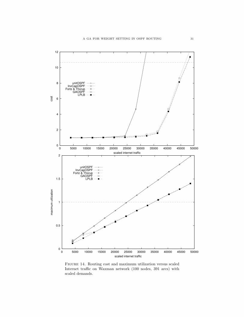
Figure 14. Routing cost and maximum utilization versus scaledInternet traffic on Waxman network (100 nodes, 391 arcs) withscaled demands.
32 M. ERICSSON, M.G.C. RESENDE, AND P.M. PARDALOS
0
2
4
6
8
10
12
0 10000 20000 30000 40000 50000 60000 70000
cost
scaled internet traffic
unitOSPFInvCapOSPF
Fortz & ThorupGAOSPF
LPLB
0
0.2
0.4
0.6
0.8
1
1.2
1.4
1.6
0 10000 20000 30000 40000 50000 60000 70000
max
imum
util
izat
ion
scaled internet traffic
unitOSPFInvCapOSPF
Fortz & ThorupGAOSPF
LPLB
Figure 15. Routing cost and maximum utilization versus scaledInternet traffic on Waxman network (100 nodes, 476 arcs) withscaled demands.
A GA FOR WEIGHT SETTING IN OSPF ROUTING 33
1
10
100
1 10 100 1000 10000
cost
CPU time (seconds on MIPS10000)
F&T solution (= 2.70)
LP lower bound (= 2.40)
Figure 16. Routing cost as a function of running time for tenindependent runs of GAOSPF on the AT&T Worldnet backbonewith total demand D = 37612.
for most instances and that better solutions can be produced if one allows longerruns of the algorithm.
A natural extension of the algorithm would be its hybridization with some localsearch, such as one similar to the local search proposed by Fortz and Thorup. Sucha local search could be applied, as in a memetic algorithm [21], to each element ofthe population at the end of each generation, or in a post-optimization phase atthe end of all generations.
A simple variant of the proposed approach can be easily implemented in parallel.
Acknowledgment
The authors wish to thank Bernard Fortz and Mikkel Thorup for sharing the testproblems as well as the shortest path code with us. Thanks also goes to JenniferRexford for many comments that greatly improved the paper.
References
[1] R.K. Ahuja, T.L. Magnanti, and J.B. Orlin. Network Flows. Prentice Hall, 1993.[2] D.O. Awduche, J. Malcolm, J. Agogbua, M. O’Dell, and J. McManus. Requirements for
traffic engineering over MPLS. Technical Report RFC 2702, Network Working Group, 1999.http://search.ietf.org/rfc/rfc2702.txt.
[3] J.C. Bean. Genetic algorithms and random keys for sequencing and optimization. ORSA J.on Computing, 6:154–160, 1994.
34 M. ERICSSON, M.G.C. RESENDE, AND P.M. PARDALOS
[4] U. Black. IP Routing Protocols, RIP, OSPF, BGP, PNNI & Cisco routing protocols. PrenticeHall, 2000.
[5] A. Bley, M. Grotchel, and R. Wesslay. Design of broadband virtual private networks: Modeland heuristics for the B-WiN. Technical Report SC 98-13, Konrad-Zuse-Zentrum fur Informa-tionstecknik Berlin, 1998. To appear in Proc. DIMACS Workshop on Robust CommunicationNetwork and Survivability, AMS-DIMACS Series.
[6] K. Calvert, M. Doar, and E.W. Zegura. Modeling internet topology. IEEE CommunicationsMagazine, 35:160–163, 1997.
[7] Cisco. Configuring OSPF. Cisco Press, 1997.[8] K.G. Coffman and A.M. Odlyzko. Internet growth: Is there a ”Moore’s Law” for data traffic?
In J. Abello, P.M. Pardalos, and M.G.C. Resende, editors, Handbook of Massive Data Sets,pages 47–93. Kluwer Academic Publishers, 2001.
[9] E. Dijkstra. A note on two problems in connection of graphs. Numerical Mathematics, 1:269–271, 1959.
[10] A. Feldmann, A. Greenberg, C. Lund, N. Reingold, and J. Rexford. NetScope: Traffic engi-neering for IP networks. IEEE Network Magazine, 14:11–19, 2000.
[11] A. Feldmann, A. Greenberg, C. Lund, N. Reingold, J. Rexford, and F. True. Deriving trafficdemands for operational IP networks: Methodology and experience. IEEE/ACM Transac-tions on Networking, 9:265–279, 2001.
[12] B. Fortz and M. Thorup. Increasing internet capacity using local search. Technical report,AT&T Labs Research, 2000. Preliminary short version of this paper published as “InternetTraffic Engineering by Optimizing OSPF weights,” in Proc. IEEE INFOCOM 2000 – TheConference on Computer Communications.
[13] D.E. Goldberg. Genetic Algorithms in Search, Optimization, and Machine Learning.Addison-Wesley, 1989.
[14] J.H. Holland. Adaptation in Natural and Artificial Systems. MIT Press, 1975.[15] R.B. Hollstein. Artificial genetic adaptatiion in computer control systems. PhD thesis, Uni-
versity of Michigan, 1971.[16] Internet Engineering Task Force. Ospf version 2. Technical Report RFC 1583, Network Work-
ing Group, 1994.[17] N.K. Karmarkar. A new polynomial–time algorithm for linear programming. Combinatorica,
4:373–395, 1984.[18] L.G. Khachiyan. A polynomial time algorithm for linear programming. Dokl. Akad. Nauk
SSSR, 244:1093–1096, 1979.[19] J.R. Koza, F.H. Bennett III, D. Andre, and M.A. Keane. Genetic Programming III, Dar-
winian Invention and Problem Solving. Morgan Kaufmann Publishers, 1999.[20] F. Lin and J. Wang. Minimax open shortest path first routing algorithms in networks support-
ing the smds services. In Proc. IEEE International Conference on Communications (ICC),volume 2, pages 666–670, 1993.
[21] P. Moscato. Memetic algorithms. In P.M. Pardalos and M.G.C. Resende, editors, Handbookof Applied Optimization. Oxford University Press, 2001.
[22] J.T. Moy. OSPF protocol analysis. Technical Report RFC 1245, Network Working Group,1991.
[23] J.T. Moy. OSPF, Anatomy of an Internet Routing Protocol. Addison-Wesley, 1998.[24] M. Rodrigues and K.G. Ramakrishnan. Optimal routing in data networks, 1994. Presentation
at International Telecommunication Symposium (ITS).[25] W. Stallings. High-Speed Networks TCP/IP and ATM Design Principles. Prentice Hall, 1998.[26] T.M. Thomas II. OSPF Network Design Solutions. Cisco Press, 1998.[27] B.M. Waxman. Routing of multipoint connections. IEEE J. Selected Areas in Communica-
tions (Special Issue on Broadband Packet Communication), 6:1617–1622, 1998.[28] E.W. Zegura. GT-ITM: Georgia Tech internetwork topology models (software), 1996.
http://www.cc.gatech.edu/fac/Ellen.Zegura/gt-itm/gt-itm.tar.gz.[29] E.W. Zegura, K.L. Calvert, and S. Bhattacharjee. How to model an internetwork. In Proc.
15th IEEE Conf. on Computer Communications (INFOCOM), pages 594–602, 1996.
A GA FOR WEIGHT SETTING IN OSPF ROUTING 35
(M. Ericsson) Department of Mathematics, Division of Optimization and Systems The-ory, Royal Institute of Technology (KTH), Stockholm, Sweden
E-mail address, M. Ericsson: [email protected]
(M.G.C. Resende) Information Sciences Research, AT&T Labs Research, 180 Park Av-enue, Room C241, Florham Park, NJ 07932 USA.
E-mail address, M.G.C. Resende: [email protected]
(P.M. Pardalos) Department of Industrial and Systems Engineering, University ofFlorida, Gainesville, FL 32611 USA.
E-mail address, P.M. Pardalos: [email protected]