A Goodness-of-Fit Approach to Estimating Equivalence Scalesftp.iza.org/dp7209.pdf · A Goodness-of-Fit Approach to Estimating Equivalence Scales . Martin Biewen . University of Tübingen,

DI

SC

US

SI

ON

P

AP

ER

S

ER

IE

S

Forschungsinstitut zur Zukunft der ArbeitInstitute for the Study of Labor

A Goodness-of-Fit Approach to EstimatingEquivalence Scales

IZA DP No. 7209

January 2013

Martin BiewenAndos Juhasz

A Goodness-of-Fit Approach to Estimating Equivalence Scales

Martin Biewen University of Tübingen,

IZA and DIW Berlin

Andos Juhasz University of Tübingen

Discussion Paper No. 7109 February 2013

IZA

P.O. Box 7240 53072 Bonn

Germany

Phone: +49-228-3894-0 Fax: +49-228-3894-180

E-mail: [email protected]

Any opinions expressed here are those of the author(s) and not those of IZA. Research published in this series may include views on policy, but the institute itself takes no institutional policy positions. The IZA research network is committed to the IZA Guiding Principles of Research Integrity. The Institute for the Study of Labor (IZA) in Bonn is a local and virtual international research center and a place of communication between science, politics and business. IZA is an independent nonprofit organization supported by Deutsche Post Foundation. The center is associated with the University of Bonn and offers a stimulating research environment through its international network, workshops and conferences, data service, project support, research visits and doctoral program. IZA engages in (i) original and internationally competitive research in all fields of labor economics, (ii) development of policy concepts, and (iii) dissemination of research results and concepts to the interested public. IZA Discussion Papers often represent preliminary work and are circulated to encourage discussion. Citation of such a paper should account for its provisional character. A revised version may be available directly from the author.

mailto:[email protected]

IZA Discussion Paper No. 7109 February 2013

ABSTRACT

A Goodness-of-Fit Approach to Estimating Equivalence Scales1 We use income satisfaction data in order to estimate equivalence scales. Our method differs from previous attempts to use satisfaction data for this purpose in that it can be used to estimate or evaluate any given parametric equivalence scale. It can also be employed to investigate specific questions related to equivalence scales such as whether these scales are income-dependent or to what extent they depend on specific household characteristics such as whether some household members are in a partner relationship. A further advantage of our approach is that, within a first-differencing nonlinear least-squares framework, we can carry out full statistical inference about the hypotheses under consideration. Our empirical results suggest that household economies of scale are higher than those assumed in commonly used scales such as the OECD or the Luxembourg scale. We also obtain the novel empirical result that economies of scale may decrease (rather than increase) in income, which is what one would expect if the share of consumption goods generating economies of scale (such as housing) decreases with income. JEL Classification: J31, J71, C02, D31 Keywords: income satisfaction, economies of scale, nonlinear least squares Corresponding author: Martin Biewen Department of Economics University of Tübingen Mohlstr. 36 72074 Tübingen Germany E-mail: [email protected]

1 We are grateful to Andrew Oswald for helpful discussions and suggestions, and to Carsten Schröder for help with the literature. The data used in this paper (SOEP v27, 1998-2010) were made available by the German Socio-Economic Panel Study (SOEP) at the German Institute for Economic Research (DIW), Berlin

mailto:[email protected]

1 Introduction

Equivalence scales are used to make the utility of income comparable across heterogeneous house-

holds. They thus play a crucial role in various fields of welfare and public economics such as the

measurement of inequality and poverty, or the design of tax- and welfare systems. In principle,

three main approaches have been used to construct or estimate equivalence scales.2 The first

approach is based on the estimation of consumer demand systems (see, e.g., Muellbauer, 1980,

Pashardes, 1995, and Pendakur, 1999). As shown by Blundell/Lewbel (1991), this approach is

challenged by identification problems unless additional assumptions are made. One such assump-

tion is that the equivalence scale is independent of reference income (‘Independence of Base

Assumption’, Lewbel, 1989, Blackorby/Donaldson, 1993). More general restrictions have been

suggested by Donaldson/Pendakur (2003, 2006). A second approach is based on subjective data

on income or life satisfaction. In one variant, this approach uses survey data that directly lets

respondents describe which income levels they associate with different levels of welfare (e.g., van

Praag, 1968, 1991, Kapteyn/van Praag, 1976, Koulovatianos et al., 2005). A drawback of this

approach is that respondents are asked to make assessments of situations that may be hypo-

thetical to them. This drawback is not present in the second variant of the subjective approach

which only uses information on how satisfied respondents are with their own factual income (e.g.,

Melenberg/van Soest, 1996, Bellemare et al. 2002, Schwarze, 2003, and Bollinger et al., 2012).

The third approach to constructing equivalence scales is an ad-hoc one. It uses ‘expert’ assess-

ments or more or less arbitrary rules-of-thumb in order to define the weights different household

members receive in the equivalence scale. Examples are the so-called OECD equivalence scale or

the Luxembourg (= square-root) equivalence scale (see Atkinson et al., 1995, or OECD, 2005).

Although this latter approach is less evidence-based than the first two approaches, the equivalence

scales resulting from it are by far the most widely used ones in practice.

In this paper, we contribute to the second line of research, i.e. we use income satisfaction data

in order to estimate equivalence scales. Our approach differs from previous approaches in that

it can be used to estimate or evaluate any parametric equivalence scale. We use the simple

idea that there should be some relationship between income satisfaction and equivalized income,

i.e. the household income as perceived by an individual in a household with a given structure.

This relationship will only be correctly specified if the correct equivalence scale is used in order

to compute equivalized income from household income. As the correctly equivalized income is

2See Lewbel/Pendakur (2008a) and Schröder (2009) for overviews.

1

a nonlinear function of the equivalence scale, this leads to a nonlinear least squares problem

which we implement on first-differenced data in order to eliminate time-invariant unobserved

heterogeneity.3 Given the parametric nature of our procedure, we can carry out full statistical

inference about equivalence scale parameters and related hypotheses such as whether equivalence

scales are income dependent or how they depend on specific household features. For example,

we can test whether the exact ages of household members matter, or whether the equivalence

scale crucially depends on whether some of the household members are partners. The latter was

suggested by Bollinger et al. (2012) who argue that in this case, household economies of scale

should be much higher because partners are likely to share the same room, the same bed etc.

Our empirical results suggest that commonly used equivalence scales such as the OECD equiv-

alence scale or the Luxembourg equivalence scale underestimate household economies of scale.

The economies of scale of living together in a household as perceived by the household members

in terms of income satisfaction appear to be substantially higher than for example embodied in

the square-root rule provided by Luxembourg equivalence scale. As in Bollinger et al. (2012),

we also find that the economies of scale in the case of a couple living in one household may be

very large so that in some cases ‘two can live as cheaply as one’. Contrary to some results in the

literature, we find that household economies of scale may decrease with reference income which

is what one would expect if the share of expenditures generating economies of scale (such as

housing) decreases in income. We find that this is true for adults but not for children, for whom

economies of scale increase with income to a certain extent. We also investigate how estimates

of poverty and inequality are affected if the equivalence scales resulting from our method rather

than standard equivalence scales such as the OECD or Luxembourg scale are used. We find that

using the estimated scales may make a substantial difference.

The rest of this paper is structured as follows. In section 2, we discuss some related literature.

Section 3 describes our econometric setup. Section 4 introduces the data used in our empirical

analysis. In section 5, we present our empirical results. Section 6 concludes.

3For a similar idea used in the context of poverty line estimation, see Juhasz (2012).

2

2 Related literature

We briefly review some related literature. We concentrate on contributions that either use sub-

jective income evaluation data or that are concerned with whether or not equivalence scales

are income dependent. The subjective approach to estimating equivalence scales was pioneered

by van Praag (1968) and has generated a large literature, see for example Kapteyn/van Praag

(1976), van Praag/van der Sar (1988), and van Praag (1991) (also called the ‘Leyden school’).

The idea of this approach is to use survey data in which respondents explicitly state what income

level they would consider as a) very bad, b) bad, c) insufficient, d) sufficient, e) good, and f) very

good. This data is then used to estimate a household cost function (of a particular parametric

form), which can be used to derive household equivalence scales. The equivalence scales resulting

from this method are typically quite flat, i.e. imply large economies of scale and small marginal

costs for additional household members (see the discussion in Melenberg/van Soest, 1996).

A related but different approach is followed by Koulovatianos et al. (2005) who directly ask survey

participants how they think equivalence scales look like for different levels of reference income.

They can thus directly investigate whether equivalence scales are income dependent and what

form this dependence takes. Their results suggest that equivalence scales decline with income,

implying that economies of scale are larger for richer households. Another advantage of their

approach is that they can directly test whether the relationship between equivalence scales and

income satisfies restrictions needed to identify equivalence scales from consumption data such as

‘Generalized Equivalence Exactness’ (GESE, Donaldson/Pendakur, 2003). Koulovatianos et al.

(2005) find evidence in favor of such restrictions.

Melenberg/van Soest (1996) and Bellemare et al. (2002) are two examples for studies which use

data on actual income satisfaction in order to estimate equivalence scales. The advantage of this

approach over the ones described in the previous two paragraphs is that it only uses subjective

assessments of situations the respondents actually experience rather than of situations that may

be very hypothetical to them. The focus of Melenberg/van Soest (1996) and Bellemare et al.

(2002) is on the semi-parametric modeling of the relationship between income satisfaction and

household income.4 They conclude that simple parametric models of income satisfaction like

the ordinal probit model are generally rejected in favor of more nonparametric alternatives, but

4Melenberg/van Soest (1996) also provide a comparison of the income satisfaction approach with that of the

‘Leyden school’.

3

that estimated equivalence scales do not depend much on what model and estimation method is

chosen.

Schwarze (2003) seems to be the first one to use panel data for estimating an equivalence scale

from income satisfaction data. Using panel data makes it possible to control for time-invariant

correlated unobserved heterogeneity in the determinants of income satisfaction, which appears to

be a highly relevant point. More concretely, Schwarze (2003) estimates the economies of scale

parameter in what we call a Luxembourg-type scale below by using a fixed-effects logit model

after collapsing income satisfaction into a zero/one-indicator. Schwarze’s approach is related to

the method we use below, but is restricted to the particularly simple form of the Luxembourg-type

scale (which results in a linear form after taking the log).

Bollinger et al. (2012) use panel data on both income satisfaction and general life satisfaction

in order to estimate equivalence scales. They use fixed-effects and random-effects ordered probit

and logit models in order to control for unobserved heterogeneity. Their main point is that

household economies of scale may be much larger than commonly assumed, especially if there

are partners in the household who can share goods to a much larger extent than non-partners.

Bollinger et al.’s method is less general than ours as it requires the equivalence scale to be of a

particular form in order to fit into their framework which is based on the ‘Independence of Base

Assumption’ (Lewbel, 1989, Blackorby/Donaldson, 1993).5

There is a large number of papers that have tested the ‘Independence of Base Assumption’

using consumption data and parametric or nonparametric demand systems. Parametric papers

(Blundell/Lewbel, 1991, Dickens et al., 1993, and semiparametric papers (Blundell et al., 1998,

Pendakur, 1999) generally clearly reject the independence of base assumption. The evidence in

Pendakur (1999) suggests that it may hold for some household types but not for others, especially

those with children. Donaldson/Pendakur (2003) relax the independence of base assumption by

allowing for certain kinds of dependencies between the equivalence scale and reference income

(‘Generalized Equivalence Exactness’, GESE). Although they find that their assumption of GESE

does not exactly hold in their data, their empirical results suggest that household economies of

scale increase with reference income, especially for households with children. Finally, De Ree et

al. (2013) combine the estimation of a parametric demand system with subjective data on income

satisfaction. Their results also suggest that household economies of scale increase in reference

income (or in reference utility, respectively).

5In their data, Bollinger et al. (2012) do not find evidence against this assumption.

4

The question of estimating equivalence scales is also related to a strand of the literature that,

based on collective household models, aims at identifying economies of scale and resource shares

of different household members from consumption data, see Browning et al. (2012), Lew-

bel/Pendakur (2008b), Bargain/Donni (2012), and Dunbar et al. (2013). As described in

Browning et al. (2012) and Dunbar et al. (2013), this involves difficult identification prob-

lems which are typically addressed by making assumptions that are similar to the independence

of base assumption, in particular resource shares and economies of scale are assumed to be inde-

pendent of total expenditures (Lewbel/Pendakur, 2008, Dunbar et al., 2013, and Bargain/Donni,

2012). Using subjective utility data may be a way to avoid these difficulties (but one has to be

willing to make the assumption that utility statements are comparable across persons, see below).

3 Econometric Model

The idea of our approach is quite simple. Let uit denote the income satisfaction of individual

i = 1, . . . , N in period t = 1, . . . , T . We then assume that there is a relationship between income

satisfaction, equivalent income, and possibly other determinants

uit = γ log(eqit(wit, θ)) + z′itβ + αi + εit (1)

eqit(wit, θ) = hhincit/s(wit, θ) (2)

where eqit(wit, θ) is the equivalent income of individual i in period t, zit are characteristics

that may influence income satisfaction in addition to equivalent income, αi are time-invariant

determinants of individual income satisfaction, and εit are time-variant idiosyncratic determinants.

The equivalent income eqit(wit, θ) is computed by dividing household income hhincit by an

equivalence scale s(wit, θ), which may depend on characteristics wit and parameters θ. The

purpose of the equivalence scale is to make household incomes comparable across households

with characteristics wit. Following the literature (e.g., Bellemare et al., 2002, Frijters et al.,

2004, Powdthavee, 2010, Sacks et al., 2010), we generally assume that the relationship between

income and satisfaction is logarithmic, but we also test for this within a more general isoelastic

specification and find the log-specification to be a good choice in most cases (see Layard et al.,

2008, and below).

We adopt a first differencing approach in order to eliminate unobserved time-invariant determi-

5

nants of income satisfaction αi, i.e. we base our estimations on

∆uit = γ∆ log(eqit(wit, θ)) + ∆z′itβ +∆εit. (3)

Note that (1) and (3) are nonlinear regression models because the parameters of the equivalence

scale θ enter the model through eqit(wit, θ) in a nonlinear way. In (3), the parameters (γ, β, θ) can

be consistently estimated using nonlinear least squares, if for the error term ∆εit of the equation,

E(∆εit|∆ log(eqit(wit, θ)),∆zit) = 0 (see Wooldridge (2010), assumption NLS.1). A sufficient

condition for this is that E(εit|zi, wi) = 0 with zi = (zi1, . . . , ziT ) and wi = (wi1, . . . , wiT ),

i.e. the variables wi and zi must be unrelated to the idiosyncratic determinants εit of income

satisfaction. Note that the assumption E(εit|zi, wi) = 0 leaves the relationship between the

unobserved time-invariant effects αi and all other components of the model eqit(wit, θ), zit, wit, εit

completely unrestricted, i.e. the omitted time-invariant determinants of income satisfaction αi

may be arbitrarily correlated with any of the explanatory variables or the idiosyncratic shocks εit.

We note that model (1) assumes a cardinal structure of income satisfaction. In our data (see

next section), such an assumption is easily defended as our income satisfaction variable uses a

scale with eleven points and two clearly defined end points (‘totally happy’ and ‘totally unhappy’)

such that most respondents will probably intend their answer to this survey question to be a

cardinal one. Moreover, Ferrer-i-Carbonell/Frijters (2004) have shown that results using cardinal

models generally do not differ in substantial ways from results using ordinal models. We choose

a cardinal approach because there is no easy way to take proper account of unobserved charac-

teristics αi in existing multinomial or ordinal models (Wooldridge, 2010). A possible solution to

this problem would be to collapse the satisfaction variable into a dichotomous indicator (Winkel-

mann/Winkelmann, 1998, Schwarze, 2003, Ferrer-i-Carbonell/Frijters, 2004, among others) and

to use a fixed effects logit model. This is likely to lead to a considerable drop in efficiency how-

ever, especially in our case. Another option would be to use a flexible ordered logit or probit

model with random effects (Boes/Winkelmann, 2010), which makes stronger distributional and

functional form assumptions. For these reasons, we concentrate on the fixed effects approach

described above.

One should also bear in mind that the use of satisfaction data in order to estimate equivalence

scales requires the assumption that satisfaction statements are comparable across persons. Of

course, the validity of this assumption is open to debate, but given the ‘absolute’ and ‘metric’

nature of our scale (it has got two clearly defined endpoints and a fine grid of eleven points with an

association of equal distances), it seems plausible that survey respondents attach some absolute

6

meaning to their satisfaction statements that corresponds well to how the word ‘satisfied’ is used

in society.

4 Data

We use yearly data from the German Socio-Economic Panel (SOEP). Our dependent variable

is income satisfaction, i.e. the answer to the survey question ‘How satisfied are you with your

household income’ on a scale from 0 to 10. By focussing on income satisfaction we sidestep the

problem that for more general satisfaction measures (such as satisfaction with life), a very large

number of determining factors should be taken into account (for the wide range of these factors

see Frey/Stutzer, 2002, Oswald, 2003, Blanchflower/Oswald, 2004a,b). Equivalence scales are

about equivalizing the utility assigned to income so that it seems adequate to focus on satisfaction

with income rather than on more general satisfaction measures.6

Our income measure is monthly net household income as reported by the household head at

survey time. As potential further covariates of income satisfaction we originally considered a

large number of individual and household characteristics as well as individual or household events.

We excluded variables that did not or that changed only little over time (education, region etc.)

as those are automatically controlled for in our first-differencing procedure. The list of variables

originally considered by us included age, age squared, the number of days spent ill in the previous

year, the number of months spent on unemployment benefits or social assistance in the previous

year, the degree of disability, as well as dummies indicating whether the person was unemployed

at survey time, whether there were other unemployed persons in the household, whether the

person worked part time, whether the person was married, whether the person was married but

separated, in education, retired or out of the labor force. In order to account for possible relative

effects of income satisfaction, we included quartile dummies describing the relative position of

the household in the overall distribution of household incomes.7

We also considered a number of events such as whether the person was newly married, soon

6A related view is that overall satisfaction can be decomposed into different ‘domains’, see Easterlin/Sawangfa

(2007). We also experimented with using general life satisfaction as the dependent variable but found it hard to

obtain statistically significant results.

7We generally found these dummies to be highly significant (see below). Omitting them did not change the

estimates of the equivalence scale parameters much, but they tended to be slightly lower if the quartile dummies

were not included.

7

to be married, newly divorced, soon to be divorced, whether somebody in the household had

died, whether a child recently left the household, whether there was a new born baby in the

household, or whether the person had recently become disabled. In general, we excluded all

variables whose share of nonzero changes over a period of five years was below three percent.

This applied to almost all of the events considered and to many of the other potential covariates

listed above (see results below). We also omitted in our final specifications covariates that were

grossly insignificant. In general, we found that the estimates of our equivalence scale parameters

did not depend much on whether we omitted certain covariates from our regressions. We also

included a full set of time dummies (implying that we omitted age but kept age squared as a

regressor). In order to test whether dynamic effects of income matter, we also tried out adding

the change in equivalent income ∆eqit as a regressor in (1) (i.e. we included ∆(∆eqit) in (3)).

This generally yielded a statistically insignificant coefficient and did not change any of our other

results so that we did not include ∆eqit in our final specification (similar findings were reported

in Layard et al., 2008).

Our sample consists of all individuals with non-missing information on the variables described

above. This excludes individuals under 16 years of age as SOEP questionnaires are only addressed

to individuals aged 16 years or older. Our overall sample period comprises the years 1999 to 2009.

We look at the three subperiods 1999 to 2003, 2002 to 2006, and 2005 to 2009, i.e. we estimate

(3) for each of these subperiods. In order to minimize the influence of outliers, we drop the

top percentile of income observations. We also take account of the clustering of individuals in

households and over time by computing clustered standard errors based on the original household

identifier of the survey. This means we cluster together individuals who either live together in a

given period or who are otherwise related because their households are the result of a household

split in earlier periods. This allows for arbitrary correlation within household clusters as well as

for heteroscedasticity over time (Wooldridge, 2010).

5 Empirical Results

5.1 Estimating and evaluating standard scales

In this section, we apply the framework described above to estimate and evaluate three com-

monly used scales, the Luxembourg (or square-root) scale, the (modified) OECD scale, and the

8

Banks/Johnson-scale (see Atkinson et al., 1995, OECD, 2005, and Banks/Johnson, 1994).

Luxembourg scale

The Luxembourg scale is a special case of the parametric form

s(hhsizeit, α) = (hhsizeit)α, (4)

where in the specific case of the Luxembourg scale, the economies of scale parameter α is set

to one half. We estimate (4) by treating α as a free parameter using the procedure described

above. The estimation results for α are shown in the first column of table 1. Selected results for

other regression parameters are given in the appendix (this is also true for all other specifications

reported below).

— Table 1 around here —

The estimates for the economies of scale parameter are between .28 and .34 and are statistically

significantly different from one half. The results for α are very similar to the estimates in Schwarze

(2003) who also uses SOEP data but who applies the technique of collapsing income satisfaction

into a dichotomous indicator. Note that the economies of scale suggested by these estimates is

much lower than those implied by the Luxembourg scale with α = .5.

OECD scale

Next we estimate the scale

s(hhsizeit, childrenit, a, b) = 1 + a · (hhsizeit − childrenit − 1) + b · childrenit, (5)

where childrenit the number of household members aged 14 years or younger and hhsizeit the

household size as before. The OECD equivalence scale results as a special case with a = .5 and

b = .3, i.e. the first person in the household receives a weight of one, each additional adult8 a

weight of .5 and an additional child receives a weight of .3 (an older choice was a = .7, b = .5,

see Atkinson et al., 1995). The estimates for a and b using the method described above are

shown in the second and third column of table 1. The weight for an additional adult is estimated

at around .17 to .22, that of an additional child at around .08 to .11 The hypothesis of a = .5

8In accordance with the language use associated with the OECD scale, we call household members aged 15

or older ‘adults’.

9

and b = .3 (and that of a = .7, b = .5) is clearly rejected. There also seems to be the tendency

that the estimated weight for an adult is about twice as large as that of a child.

As an illustration that our estimated equivalence scale parameters really reflect underlying struc-

tures in income satisfaction, we decompose the nonlinear least squares problem (3) in two steps.

We first estimate for given a, b linear regressions of ∆uit on ∆eqit(a, b) and ∆zit over a grid of

values for a and b. Among the regressions for all the grid points, we then choose the regression

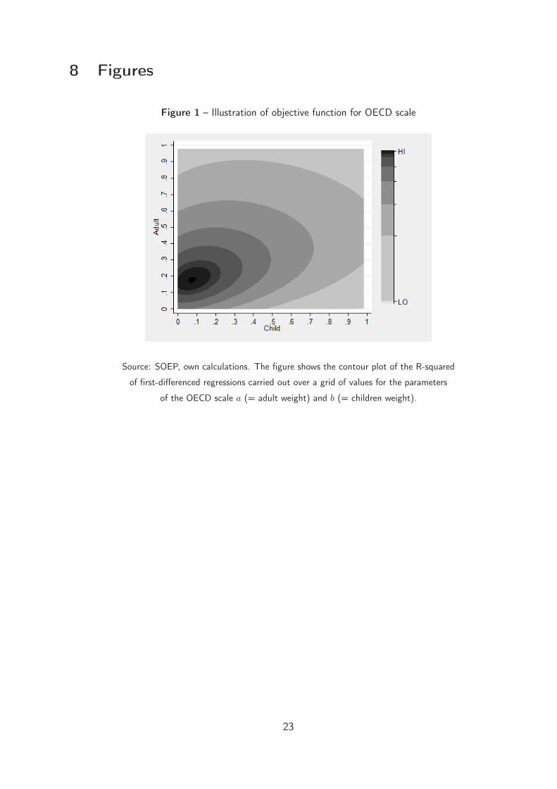
that has the best fit. Figure 1 presents the contour plot of the R-squared of such regressions

over the grid of a and b. One can see that the objective function with respect to the parameters

of the equivalence scale a and b is very well-behaved with a unique optimum at the values that

result from the nonlinear least squares procedure.

— Figure 1 around here —

Banks/Johnson scale

Another popular choice for a parametrized equivalence was suggested by Banks/Johnson (1994).

The scale is defined by

s(adultsit, childrenit, a, b) = (adultsit + η · childrenit)α, (6)

i.e. children receive a weight η when compared to adults, and the economies of scale parameter

is given by α as in the case of the Luxembourg scale. The estimation results for this scale are

shown in the last two columns of table 1. The estimated weight for children is between .4 and

.6, suggesting, as before, that the weight of a child is about half that of an adult. The estimated

economies of scale parameter is very similar to that of the Luxembourg scale. Again, we clearly

reject the hypothesis that α = .5.

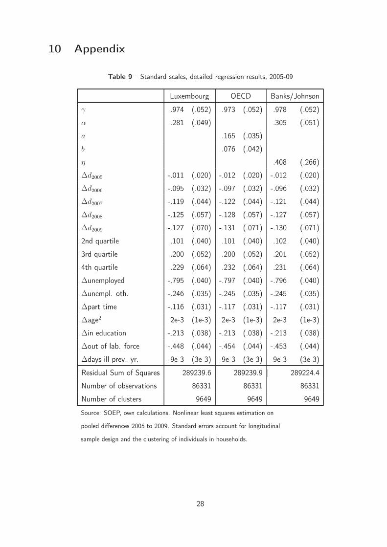
More detailed regression results for the three specifications are given in table 9. The estima-

tion results for other regressors are in line with prior expectations. Interestingly, the estimated

coefficients for the other regressors are practically invariant across the three specifications. The

fit of the different specifications as measured by the sum of squared residuals suggests that the

Banks/Johnson-scale has a slight advantage over the other two specifications.9

9It might make sense to correct for the degrees of freedom (i.e. divide by the number of observations minus the

number of estimated parameters). Given the large number of observations however, this makes little difference.

10

5.2 Iso-elastic specification

As indicated above, we check the robustness of our results with respect to the assumption that

the relationship between income satisfaction and equivalent income is a logarithmic one by nesting

the log-specification in the more general iso-elastic specification (Layard et al., 2008). Equations

(1) and (3) then change to

uit = γ ·eqit(wit, θ)

λ − 1

λ+ z′itβ + αi + εit (7)

∆uit = γ ·∆

[

eqit(wit, θ)λ − 1

λ

]

+∆z′itβ +∆εit. (8)

The iso-elastic specification assumes that marginal income satisfaction with respect to income is

constant and equal to 1− λ. The special case of the log-specification results for λ → 0.


The results for the Luxembourg scale and the OECD scale using the iso-elastic assumption are

reported in table 2 (more detailed results are given in table 10 in the appendix). In two of the cases,

the estimate for λ is slightly below zero, but not statistically significant. For the period 2005 to

2009, the estimate is more negative and statistically significant. Note however, that the estimates

of the equivalence scale parameters are very similar to those obtained in the log-specification so

that it seems insubstantial in the given context whether or not the log-specification or the more

general iso-elastic specification is chosen.

5.3 Details of the household structure

Next, we investigate the role of further household characteristics.

Age of children

We extend the OECD-type scale in order to allow for children of different ages. More specifically,

we estimate

s(hhsizeit, children05it, children613it, a, b1, b2) (9)

= 1 + a · (hhsizeit − children613it − children05it − 1)

+ b1 · children613it + b2 · children05it,

11

where children05it is the number of children aged at most five years, children613it the number

of children aged between 6 and 13 years. The results are shown in table 3 (and in table 11 in

the appendix). They indicate that the weight for younger children is indeed slightly lower than

the weight for older children but the difference is far from being significant. We conjecture that

much larger sample sizes would be required to trace out differences in equivalence weights for

children of different ages.


The role of partners in the household

Following Bollinger et al. (2012), we distinguish between household members who are in a partner

relationship and household members who are not. More specifically, we estimate

s(hhsizeit, partnersit, childrenit, a1, a2, b) (10)

= 1 + a1 · partnersit + a2 · (hhsizeit − partnersit − childrenit − 1)

+ b · childrenit (11)

where partnerit is the number of household members who are the partner of another household

member, divided by two (in order to avoid double counting). The results are shown in table 4

(and in table 11 in the appendix). The weight of an additional adult who is a partner of another

household member is estimated to be very low and statistically insignificant for the periods 1999

to 2003 and 2002 to 2006. This is similar to the results in Bollinger et al. (2012) for British data.

However, for the period 2005 to 2009, the weight of a parter is estimated higher and statistically

different from zero, although still lower than the weight of a non-partner.


5.4 Income dependency

In this section, we use different functional forms in order to test the ‘Independence of Base

Assumption’ (Lewbel, 1989, Blackorby/Donaldson, 1993), i.e. we investigate to what extent the

equivalence scale and its economies of scale depend on reference income. Our framework allows

12

us to carry out such a test as we just have to relate the equivalence scale parameters to the level

of equivalent income.10

Direct estimation Luxembourg scale

In the case of the Luxembourg-type scale

s(hhsizeit, α) = (hhsizeit)α, (12)

assume that the economies of scale parameter α is related to equivalent income as

α = α1 + α2 [log(eqit(hhsizeit, α))− log(q∗)] , (13)

where q∗ is some fixed income level. If α2 6= 0, then the economies of scale α depend either

positively or negatively on the level of reference income (= equivalent income). The parameter α1

represents the economies of scale for a particular fixed level of equivalent income q∗.11 Combining

log(eqit(hhsizeit, α)) = log(hhincit)− α log(hhsizeit) (14)

with (13) and solving for log(eqit(hhsizeit, α)) yields

log(eqit(hhsizeit, α)) =log(hhincit)− α1 log(hhsizeit)− α2 log(q

∗) log(hhsizeit)

1 + α2 log(hhsizeit), (15)

which we insert in first differenced form in (3) in order to estimate α1, α2.

The resulting estimates for α1 and α2 are shown in the first two columns of table 5 (and in table

12 in the appendix). For the period 1999 to 2003, the results suggest that economies of scale

rise with equivalent income in a statistically significant way. For 2002 to 2006 and for 2005 to

2009, the dependency on equivalent income is weaker and only marginally significant. The result

for 1999 to 2003 suggests that a ten percent increase in equivalent income is associated with an

increase of the economies of scale parameter α of around .0336 because

α2 = .336 =∂α

∂ log(eqit)=

∂α∂eqiteqit

=.0336

10

100

=.0336

10%. (16)

This is a small but discernible effect.

10Unfortunately, there seems to be no easy way to test more general restrictions such as ‘Generalized Equivalence

Exactness’ (GESE, Donaldson/Pendakur, 2003).

11This could be any income level of interest, for example 1000 Euros or 2000 Euros. Below, we will set q∗ to

the pooled median of equivalized incomes in the respective 5-year window.

13


Iterative estimation Luxembourg scale

Specifying the relationship between the economies of scale parameter α and the equivalent income

as logarithmic, we were able to obtain a closed form expression for log(eqit), which we could

insert in our estimation equation. For other specifications, this is not possible. If we assume

equivalence scale parameters to be dependent on equivalent income, we face the problem that

equivalent income in turn depends on the equivalence scale parameters. In order to solve that

problem, we pursue an iterative approach.

We first apply this to a linear (rather than log-linear) specification of the relationship between

the economies of scale parameter of the Luxembourg scale

α = α1 + α2

[

eqit(hhsizeit, α)

1000−

q∗

1000

]

. (17)

Again, α1 is the economies of scale parameter for an equivalent income of q∗ and α2 describes by

what amount the economies of scale parameter α changes if equivalent income changes by 1000

Euros. In order to estimate α1 and α2, we use the following iterative procedure. We start with

initial values α0

1and α0

2for α1 and α2 and use these initial values to compute for each individual

their equivalent income eqit(hhsizeit, α0

1, α0

2). Using this equivalent income, we carry out the

nonlinear least squares estimation procedure to obtain new estimates α1

1and α1

2. We use these

new values for α1 and α2 to compute a new estimate of eqit(hhsizeit, α1

1, α1

2) for each individual,

which we insert in another round of nonlinear least squares estimation to obtain new estimates

α2

1and α2

2, and so on. Doing this, our estimates for α1 and α2 converge very quickly to values

that we report in the last two columns of table 5.

The resulting estimates for α1 are very similar to the ones of the log-linear specification and

correspond well to the general estimate for the economies of scale parameter of the Luxembourg

scale in the case without income dependency. The estimates for α2 are also positive, suggesting

a negative relationship between economies of scale and equivalent income as before. As in the

log-linear case, we also observe a falling tendency of the income dependency parameter, but this

time, they are statistically significant for all years.12 Taking the estimate for the period 2002 to

12Note that, due to the iterative procedure, the standard errors are only approximate. Given their very small

size and the fact that they practically do not differ from those of a one-step estimate, it seems unlikely that any

correction would change the finding that α2 is significantly different from zero.

14

2006, we obtain the result that the economies of scale parameter α grows by .077 if the equivalent

income increases by 1000 Euros. Again, this is a small but discernible effect.

Iterative estimation OECD scale

We apply the same idea to the OECD-type scale in which we make the weights for adults and

for children dependent on equivalent income, i.e.

a = a1 + a2

[

eqit(hhsizeit, childrenit, a, b)

1000−

q∗

1000

]

(18)

b = b1 + b2

[

eqit(hhsizeit, childrenit, a, b)

1000−

q∗

1000

]

. (19)

The results are reported in table 6. Again, we generally observe that the weight for additional

household members increases with rising equivalent income, i.e. the economies of scale are falling

in income. However, this is only true for adults. For children, there is the opposite effect, i.e.

the weight of an additional child decreases with income.13


How can these patterns be explained? For additional adults, we find that economies of scale are

falling in income. A possible reason is that the budget share of goods that exhibit particularly

high economies of scale (housing, cars, household appliances etc.) tend to be falling in income.

Another reason could be that the consumption behavior of richer households may be characterized

to a larger extent by individualized consumption patterns (everyone has their own room, car etc.)

which, by definition, results in a lower degree of sharing. To put it differently, poorer households

may feel a stronger necessity to spend their income on sharable goods in order to reach a decent

standard of living. On the other hand, we find the reverse result of rising economies of scale for

children. A possible explanation is that a larger number of children (i.e. two or three children

instead of just one) usually goes hand in hand with a more family oriented way of living in which

family activities (going on holiday together, eating out in expensive restaurants etc.) play a larger

role. Richer households may be in a better situation to finance such common activities. As the

results in table 7 show, the combined effect of adults and children lead to economies of scale that

are rising in income for households with two or more children.

13We also tried including in (18) an interaction term between the term in brackets and the number of children,

but this interaction term was very insignificant.

15

Our result that economies of scale may be decreasing (rather than increasing or being con-

stant) in income for childless households is in contrast to some results in the literature (Donald-

son/Pendakur, 2003, Koulovatianos et al., 2005, De Ree et al., 2013). For example, by directly

asking respondents how they think equivalence scales should vary with income, Koulovatianos et

al. (2005) find that economies of scale are larger for higher incomes. The results in Donald-

son/Pendakur (2003) based on the full estimation of a consumer demand system suggest rising

economies of scale for households with children and constant (or slightly rising) economies of

scale for childless households. These latter results are not so different from ours, especially in

that households with children experience rising economies of scale (also see table 7 and the dis-

cussion below). Using data for Indonesia and not distinguishing between adults and children, De

Ree et al. (2013) also find that economies of scale rise with reference income. Overall, there are

huge methodological and data differences between our study and these contributions so that it is

hard to assess why results differ. All we can say is that our results represent an additional piece of

evidence about the possible income dependency of equivalence scales which may be of particular

interest as it is based on direct satisfaction statements without reference to consumption data or

assumptions such as utility maximization.

5.5 Consequences for inequality and poverty

Table 7 lists the resulting equivalence scales for different household types. As already discussed

above, there are considerable differences between the official Luxembourg and OECD scales and

their estimated counterparts. The estimated Banks/Johnson scale is very similar to the estimated

OECD scale, which is remarkable given their very different structure. The results for the scale

with a special role for partners (averaged over all households in the sample), reflect the fact that

a second adult in the household is often a partner, while a third one is one who is not a partner

of another household member. This results in a discernible jump in the scale between the second

and the third adult, while the addition of a second adult is mostly associated with only a small

increase in weight. Finally, the last nine rows of table 7 demonstrate how economies of scale

vary with income. The results for the linear and log-linear specification of the Luxembourg scale

are very similar, which is reassuring as it shows that our estimates are robust with respect to

functional form specification. The last three rows of table 7 show the results where the income-

dependency of the scale may vary between adults and children. It can be seen that this generally

results in rising economies of scale for households with up to one child, but falling economies of

16

scale for households with two ore more children. Note that this to a certain extent reconciles

our results with those in Donaldson/Pendakur (2003) for Canada who also find that equivalence

scales for household with children significantly fall in income.


In table 8, we investigate how estimates of standard inequality and poverty measures are changed

if we use our estimated scales instead of the OECD or Luxembourg scale. The shift in mean

and median equivalized income shown in the first two columns of the table reflects the general

differences in economies of scale across the different scales. Economies of scale are higher for the

estimated scales than for the standard OECD and Luxembourg scales, leading to considerably

higher values for mean and median equivalized income. As discussed above, economies of scale

are particularly high for the scale incorporating the effect of partners living in the household. The

last two columns show the effect on the Gini coefficient, the mean logarithmic deviation, and

the Theil coefficient. It turns out that the differences in estimated inequality levels between the

standard scales (see the first two rows of table 8) and their estimated counterparts are surprisingly

small (rows three to five). The differences are much larger however, if we compare the standard

scales to the income dependent scales (last three rows in table 8). In the case of the income

dependent scales, inequality is considerably lower. The obvious reason for this is that in our

results, economies of scale generally decrease in income so that poorer households benefit more

from them than richer ones, narrowing the gap between the lower and the upper part of the

distribution. We do find increasing economies of scale for households with two or more children,

but these households represent only a minority of the population.


The second column table 8 shows the results for the poverty rate. We set the poverty line to the

conventional value of 60 percent of the median. As this is a relative definition of poverty, a shift in

household economies of scale has two different effects: one on the poverty line (via the median),

and one on the position of households in the population. It is therefore not surprising that the

estimated standard scales (rows three to five in table 8) which imply higher economies of scale

than the official versions (rows one and two) increase the measured poverty rate as they mainly

lift the poverty line upwards (via a higher median). In the case of the income dependent scales,

the positional effect on households dominates, i.e. low income households generally benefit more

17

from household economies of scale than richer ones, leading to a lower fraction of households

below the poverty line.

6 Conclusion

In this paper, we explore a new way to use income satisfaction data in order to estimate equiva-

lence scales. Our approach differs from previous attempts to use satisfaction data for this purpose

in that it directly considers the relationship between income satisfaction and the correctly equiv-

alized household income. Our method makes it easy to test commonly used parametric forms of

equivalence scales and to investigate specific properties such as the dependence of the scale on

reference income or on further household characteristics. Our implementation using data from

the German Socio-Economic Panel suggests that household economies of scale are higher than

those in commonly used scales such as the OECD or the Luxembourg scale. We also confirm

the hypothesis put forward by Bollinger et al. (2012) that economies of scale are particularly

high if some of the household members are in a partner relationship. Finally, we obtain the

novel empirical result that household economies of scale may decrease (rather than increase or

be constant) in income. We also investigate the consequences of using our method on measures

of poverty and inequality. These seem to be relatively limited in the case of income independent

equivalence scales but substantial if equivalence scales may depend on income.

18

7 Literature

Atkinson, A.B., L. Rainwater, and T.M. Smeeding (1995): Income Distribution in OECD Coun-

tries, OECD Social Policy Studies, No. 18, Paris.

Banks, J., P. Johnson (1994): Equivalence Scale Relativities Revisited, Economic Journal, Vol.

104, 883-890.

Bargain, O., O. Donni (2012): Expenditure on Children: A Rothbarth-Type Method Consistent

with Scale Economies and Parents, European Economic Review, Vol. 56 (4), 792-813.

Bellemare, C., B. Melenberg and A. van Soest (2002): Semi-parametric models for satisfaction

with income, Portuguese Economic Journal, Vol. 1, 181-203.

Blackorby, C, D. Donaldson (1993): Adult-equivalence scales and the economic implementation

of interpersonal comparisons of well-being, Social Choice and Welfare, Vol. 10, 335-361.

Blanchflower, D., A. Oswald (2004a): Well-Being Over Time in Britain and the USA, Journal of

Public Economics, Vol. 88, 1359-1386.

Blanchflower, D., A. Oswald (2004b): Money, Sex, and Happiness: An Empirical Study, Scandi-

navian Journal of Economics, Vol. 106, 393-416.

Blundell, R., Lewbel, A. (1991): The information content of equivalence scales, Journal of

Econometrics, Vol. 50, 49-68.

Blundell, R., A. Duncan, K. Pendakur (1998): Semiparametric estimation of consumer demand,

Journal of Applied Econometrics, Vol. 13, 435-461.

Boes, S., R. Winkelmann (2010): The Effect of Income on General Satisfaction and Dissatisfac-

tion, Social Indicators Research, Vol. 25, 111-128.

Bollinger, C.R., C. Nicoletti, and S. Pudney (2012): Two can live as cheaply as one ... but three

is a crowd, ISER Discussion Paper No. 2012-10, Institute for Social and Economic Research,

University of Essex.

Browning, M., P.A. Chiappori, A. Lewbel (2012): Estimating Consumption Economies of Scale,

Adult Equivalence Scales, and Household Bargaining Power, Working Paper, Boston College.

De Ree, J., R. Alessi, M. Pradhan (2013): The price and utility dependence of equivalence scales:

19

Evidence from Indonesia, Journal of Public Economics, Vol. 97, 272-281.

Dickens, R., V. Fry, P. Pashardes (1993): Nonlinearities, aggregation and equivalence scales,

Economic Journal, Vol. 103, 359-368.

Donaldson, D., K. Pendakur (2003): Equivalent-Expenditure Functions and Expenditure-

Dependent Equivalence Scales, Journal of Public Economics, Vol. 88, 175-208.

Donaldson, D., K. Pendakur (2006): The Identification of Fixed Costs From Consumer Behaviour,

Journal of Business and Economic Statistics, Vol. 24, 255-265.

Dunbar, G., A. Lewbel, K. Pendakur (2013): Children’s Resources in Collective Households:

Identification, Estimation and an Application to Child Poverty in Malawi, forthcoming American

Economic Review

Easterlin, R.A., W. Sawangfa (2007): Happiness and Domain Satisfaction, Theory and Evidence,

IZA Discussion Paper No. 2584, Institute for the Study of Labor, Bonn.

Ferrer-i-Carbonell, A., P. Frijters (2004): How Important Is Methodology for the Estimates of

the Determinants of Happiness?, Economic Journal, Vol. 114, 641-59.

Frey, B.S., A. Stutzer (2002): Happiness and Economics: How the Economy and Institutions

Affect Human Wellbeing, Princeton University Press.

Frijters, P., J.P. Haisken-DeNew, and M.A. Shields (2004): Money does matter! Evidence from

increasing real income and life satisfaction in East Germany following reunification, American

Economic Review, Vol. 94, 730-740.

Juhasz, A. (2012): A Satisfaction-Driven Poverty Line - A Bustle around the Poverty Line,

SOEPpaper No. 461, DIW Berlin.

Kapteyn, A., B. van Praag (1976): A New Approach to the Construction of Family Equivalence

Scales, European Economic Review, Vol. 7, 313-335.

Koulovatianos, C., U. Schmidt, and C. Schröder (2005): On the Income Dependence of Equiva-

lence Scales, Journal of Public Economics, Vol. 89, 967-996.

Layard, R., G. Mayraz, and S. Nickell (2008): The marginal utility of income, Journal of Public

Economics, Vol. 92, 1846-1857.

20

Lewbel, A. (1989): Household Equivalence Scales and Welfare Comparisons, Journal of Public

Economics, Vol. 39, 377-391.

Lewbel, A., K. Pendakur (2008a): Equivalence Scales, in: Durlauf, S., L. Blume, The New

Palgrave Dictionary of Economics, 2nd Edition, Palgrave Macmillan.

Lewbel, A., K. Pendakur (2008b): Estimation of Collective Household Models with Engel Curves,

Journal of Econometrics, Vol. 147, 350-358.

Melenberg, C., A. van Soest (1996): Semiparametric estimation of equivalence scales using

subjective information, in Nyhus, E, S.V. Troye (eds.), Frontiers in Economic Psychology - 20th

IAREP conference, IAREP, Bergen, 500-514.

Muellbauer, J. (1980): The Estimation of the Prais-Houthakker Model of Equivalence Scales,

Econometrica, Vol. 48, 153-176.

OECD (2005): What are equivalence scales?, available at www.oecd.org/dataoecd/61/52/-

35411111.pdf.

Oswald, A. (2003): How Much do External Factors Affect Wellbeing? A Way to Use ’Happiness

Economics’ to Decide", The Psychologist, Vol. 16, 140-141.

Pashardes, P. (1995): Equivalence Scales in a Rank-3 Demand System, Journal of Public Eco-

nomics, Vol. 58, 143-158.

Pendakur, K. (1999): Estimates and tests of base-independent equivalence scales, Journal of

Econometrics, Vol. 88, 1-40.

Sacks, D.W., B. Stevenson, J. Wolfers (2010): Subjective Well-Being, Economic Development

and Growth, NBER Working Paper, No. 16441, National Bureau of Economic Research.

Schröder, C. (2009): The Construction and Estimation of Equivalence Scales and Their Uses, in:

Slottje, D. (Ed.), Quantifying Consumer Preferences, Contributions to Economic Analysis, 288,

Emerald, Bingley.

Schwarze, J. (2003): Using Panel Data on Income Satisfaction to estimate Equivalence Scale

Elasticity, Review of Income and Wealth, Vol. 3, 359-372.

van Praag, B. (1968): Individual welfare functions and consumer behavior, North- Holland,

Amsterdam.

21

van Praag, B. (1991): Ordinal and Cardinal Utility: an integration of the two dimensions of the

welfare concept, Journal of Econometrics, Vol. 50, 69-89.

van Praag, B., N.L. van der Sar (1988): Household cost functions and equivalence scales, Journal

of Human Resources, Vol. 23, 193-210.

Winkelmann, L. and Winkelmann, R. (1998): Why are the unemployed so unhappy? Evidence

from panel data, Economica, Vol. 65, 1-15

Wooldridge, J.M. (2010):Econometric Analysis of Cross-Section and Panel Data, 2nd edition,

MIT Press, Cambridge.

22

8 Figures

Figure 1 – Illustration of objective function for OECD scale

Source: SOEP, own calculations. The figure shows the contour plot of the R-squared

of first-differenced regressions carried out over a grid of values for the parameters

of the OECD scale a (= adult weight) and b (= children weight).

23

9 Tables

Table 1 – Results for standard scales

Luxembourg OECD Banks/Johnson

α a (adult) b (children) η (children) α

1999-03 .321 (.052) .198 (.040) .107 (.044) .622 (.274) .341 (.055)

2002-06 .341 (.055) .218 (.043) .102 (.048) .510 (.251) .364 (.057)

2005-09 .281 (.049) .165 (.035) .076 (.042) .408 (.266) .305 (.051)

Source: SOEP, own calculations. Standard errors account for

longitudinal sample design and household clustering.

Table 2 – Results for Luxembourg and OECD scale using iso-elastic specification

Luxembourg OECD

α λ a (adult) b (children) λ

1999-03 .304 (.053) -.117 (.105) .182 (.040) .117 (.045) -.112 (.103)

2002-06 .332 (.056) -.124 (.104) .208 (.043) .122 (.051) -.115 (.101)

2005-09 .277 (.051) -.263 (.067) .151 (.037) .119 (.050) -.253 (.067)



Table 3 – Details of household structure: age of children

a (adult) b1 (6-13y.) b2 (0-5y.)

1999-03 .201 (.041) .125 (.051) .080 (.050)

2002-06 .221 (.044) .116 (.055) .081 (.057)

2005-09 .171 (.036) .100 (.048) .039 (.049)



24

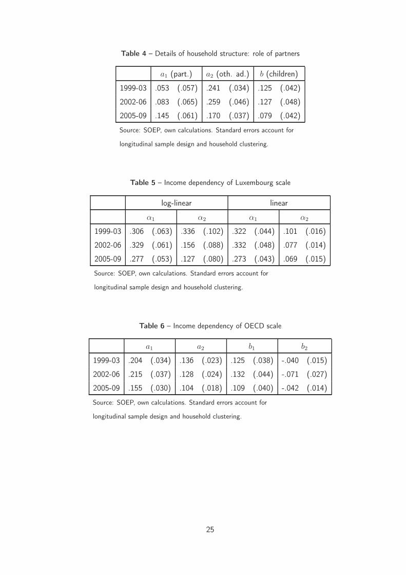
Table 4 – Details of household structure: role of partners

a1 (part.) a2 (oth. ad.) b (children)

1999-03 .053 (.057) .241 (.034) .125 (.042)

2002-06 .083 (.065) .259 (.046) .127 (.048)

2005-09 .145 (.061) .170 (.037) .079 (.042)



Table 5 – Income dependency of Luxembourg scale

log-linear linear

α1 α2 α1 α2

1999-03 .306 (.063) .336 (.102) .322 (.044) .101 (.016)

2002-06 .329 (.061) .156 (.088) .332 (.048) .077 (.014)

2005-09 .277 (.053) .127 (.080) .273 (.043) .069 (.015)



Table 6 – Income dependency of OECD scale

a1 a2 b1 b2

1999-03 .204 (.034) .136 (.023) .125 (.038) -.040 (.015)

2002-06 .215 (.037) .128 (.024) .132 (.044) -.071 (.027)

2005-09 .155 (.030) .104 (.018) .109 (.040) -.042 (.014)



25

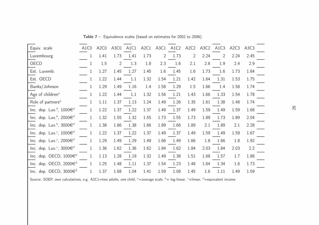
Table 7 – Equivalence scales (based on estimates for 2002 to 2006)

Equiv. scale A1C0 A2C0 A3C0 A1C1 A2C1 A3C1 A1C2 A2C2 A3C2 A1C3 A2C3 A3C3

Luxembourg 1 1.41 1.73 1.41 1.73 2 1.73 2 2.24 2 2.24 2.45

OECD 1 1.5 2 1.3 1.8 2.3 1.6 2.1 2.6 1.9 2.4 2.9

Est. Luxemb. 1 1.27 1.45 1.27 1.45 1.6 1.45 1.6 1.73 1.6 1.73 1.84

Est. OECD 1 1.22 1.44 1.1 1.32 1.54 1.21 1.42 1.64 1.31 1.53 1.75

Banks/Johnson 1 1.29 1.49 1.16 1.4 1.58 1.29 1.5 1.66 1.4 1.58 1.74

Age of childrena 1 1.22 1.44 1.1 1.32 1.56 1.21 1.43 1.66 1.33 1.54 1.78

Role of partnersa 1 1.11 1.37 1.13 1.24 1.49 1.26 1.35 1.61 1.38 1.48 1.74

Inc. dep. Lux.b, 1000ed 1 1.22 1.37 1.22 1.37 1.49 1.37 1.49 1.59 1.49 1.59 1.68

Inc. dep. Lux.b, 2000ed 1 1.32 1.55 1.32 1.55 1.73 1.55 1.73 1.89 1.73 1.89 2.04

Inc. dep. Lux.b, 3000ed 1 1.38 1.66 1.38 1.66 1.89 1.66 1.89 2.1 1.89 2.1 2.28

Inc. dep. Lux.c, 1000ed 1 1.22 1.37 1.22 1.37 1.49 1.37 1.49 1.59 1.49 1.59 1.67

Inc. dep. Lux.c, 2000ed 1 1.29 1.49 1.29 1.49 1.66 1.49 1.66 1.8 1.66 1.8 1.92

Inc. dep. Lux.c, 3000ed 1 1.36 1.62 1.36 1.62 1.84 1.62 1.84 2.03 1.84 2.03 2.2

Inc. dep. OECD, 1000ed 1 1.13 1.28 1.19 1.32 1.49 1.38 1.51 1.68 1.57 1.7 1.88

Inc. dep. OECD, 2000ed 1 1.25 1.48 1.11 1.37 1.54 1.23 1.48 1.64 1.34 1.6 1.73

Inc. dep. OECD, 3000ed 1 1.37 1.68 1.04 1.41 1.59 1.08 1.45 1.6 1.11 1.49 1.59

Source: SOEP, own calculations, e.g. A2C1=two adults, one child, a=average scale, b= log-linear, c=linear, d=equivalent income

26

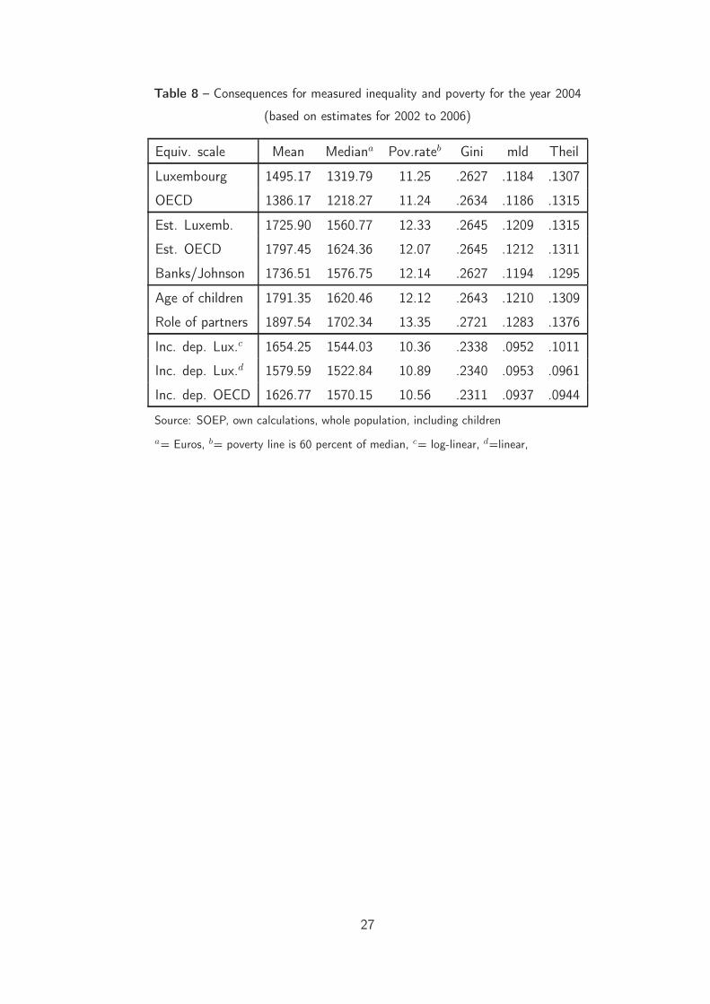
Table 8 – Consequences for measured inequality and poverty for the year 2004

(based on estimates for 2002 to 2006)

Equiv. scale Mean Mediana Pov.rateb Gini mld Theil

Luxembourg 1495.17 1319.79 11.25 .2627 .1184 .1307

OECD 1386.17 1218.27 11.24 .2634 .1186 .1315

Est. Luxemb. 1725.90 1560.77 12.33 .2645 .1209 .1315

Est. OECD 1797.45 1624.36 12.07 .2645 .1212 .1311

Banks/Johnson 1736.51 1576.75 12.14 .2627 .1194 .1295

Age of children 1791.35 1620.46 12.12 .2643 .1210 .1309

Role of partners 1897.54 1702.34 13.35 .2721 .1283 .1376

Inc. dep. Lux.c 1654.25 1544.03 10.36 .2338 .0952 .1011

Inc. dep. Lux.d 1579.59 1522.84 10.89 .2340 .0953 .0961

Inc. dep. OECD 1626.77 1570.15 10.56 .2311 .0937 .0944

Source: SOEP, own calculations, whole population, including children

a= Euros, b= poverty line is 60 percent of median, c= log-linear, d=linear,

27

10 Appendix

Table 9 – Standard scales, detailed regression results, 2005-09

Luxembourg OECD Banks/Johnson

γ .974 (.052) .973 (.052) .978 (.052)

α .281 (.049) .305 (.051)

a .165 (.035)

b .076 (.042)

η .408 (.266)

∆d2005 -.011 (.020) -.012 (.020) -.012 (.020)

∆d2006 -.095 (.032) -.097 (.032) -.096 (.032)

∆d2007 -.119 (.044) -.122 (.044) -.121 (.044)

∆d2008 -.125 (.057) -.128 (.057) -.127 (.057)

∆d2009 -.127 (.070) -.131 (.071) -.130 (.071)

2nd quartile .101 (.040) .101 (.040) .102 (.040)

3rd quartile .200 (.052) .200 (.052) .201 (.052)

4th quartile .229 (.064) .232 (.064) .231 (.064)

∆unemployed -.795 (.040) -.797 (.040) -.796 (.040)

∆unempl. oth. -.246 (.035) -.245 (.035) -.245 (.035)

∆part time -.116 (.031) -.117 (.031) -.117 (.031)

∆age2 2e-3 (1e-3) 2e-3 (1e-3) 2e-3 (1e-3)

∆in education -.213 (.038) -.213 (.038) -.213 (.038)

∆out of lab. force -.448 (.044) -.454 (.044) -.453 (.044)

∆days ill prev. yr. -9e-3 (3e-3) -9e-3 (3e-3) -9e-3 (3e-3)

Residual Sum of Squares 289239.6 289239.9 | 289224.4

Number of observations 86331 86331 86331

Number of clusters 9649 9649 9649

Source: SOEP, own calculations. Nonlinear least squares estimation on

pooled differences 2005 to 2009. Standard errors account for longitudinal

sample design and the clustering of individuals in households.

28

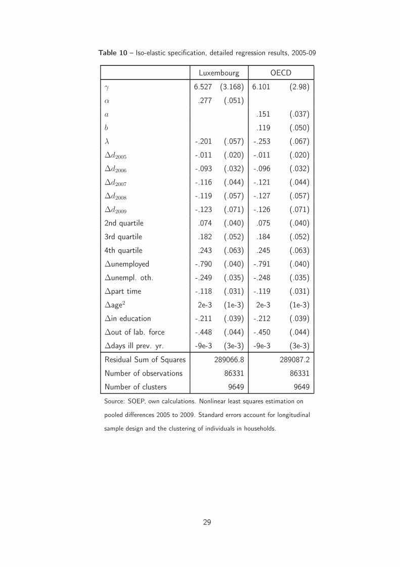
Table 10 – Iso-elastic specification, detailed regression results, 2005-09

Luxembourg OECD

γ 6.527 (3.168) 6.101 (2.98)

α .277 (.051)

a .151 (.037)

b .119 (.050)

λ -.201 (.057) -.253 (.067)

∆d2005 -.011 (.020) -.011 (.020)

∆d2006 -.093 (.032) -.096 (.032)

∆d2007 -.116 (.044) -.121 (.044)

∆d2008 -.119 (.057) -.127 (.057)

∆d2009 -.123 (.071) -.126 (.071)

2nd quartile .074 (.040) .075 (.040)

3rd quartile .182 (.052) .184 (.052)

4th quartile .243 (.063) .245 (.063)

∆unemployed -.790 (.040) -.791 (.040)

∆unempl. oth. -.249 (.035) -.248 (.035)

∆part time -.118 (.031) -.119 (.031)

∆age2 2e-3 (1e-3) 2e-3 (1e-3)

∆in education -.211 (.039) -.212 (.039)

∆out of lab. force -.448 (.044) -.450 (.044)

∆days ill prev. yr. -9e-3 (3e-3) -9e-3 (3e-3)

Residual Sum of Squares 289066.8 289087.2

Number of observations 86331 86331

Number of clusters 9649 9649




29

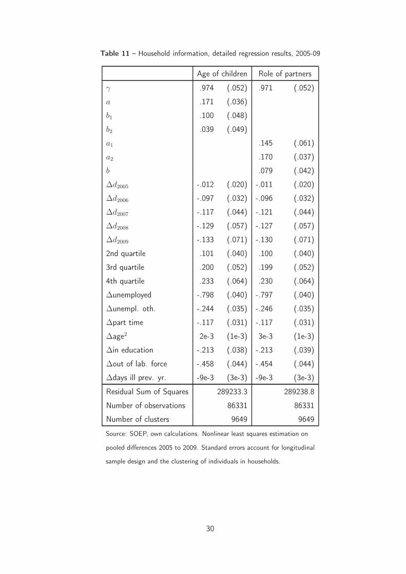
Table 11 – Household information, detailed regression results, 2005-09

Age of children Role of partners

γ .974 (.052) .971 (.052)

a .171 (.036)

b1 .100 (.048)

b2 .039 (.049)

a1 .145 (.061)

a2 .170 (.037)

b .079 (.042)

∆d2005 -.012 (.020) -.011 (.020)

∆d2006 -.097 (.032) -.096 (.032)

∆d2007 -.117 (.044) -.121 (.044)

∆d2008 -.129 (.057) -.127 (.057)

∆d2009 -.133 (.071) -.130 (.071)

2nd quartile .101 (.040) .100 (.040)

3rd quartile .200 (.052) .199 (.052)

4th quartile .233 (.064) .230 (.064)

∆unemployed -.798 (.040) -.797 (.040)

∆unempl. oth. -.244 (.035) -.246 (.035)

∆part time -.117 (.031) -.117 (.031)

∆age2 2e-3 (1e-3) 3e-3 (1e-3)

∆in education -.213 (.038) -.213 (.039)

∆out of lab. force -.458 (.044) -.454 (.044)

∆days ill prev. yr. -9e-3 (3e-3) -9e-3 (3e-3)

Residual Sum of Squares 289233.3 289238.8

Number of observations 86331 86331

Number of clusters 9649 9649




30

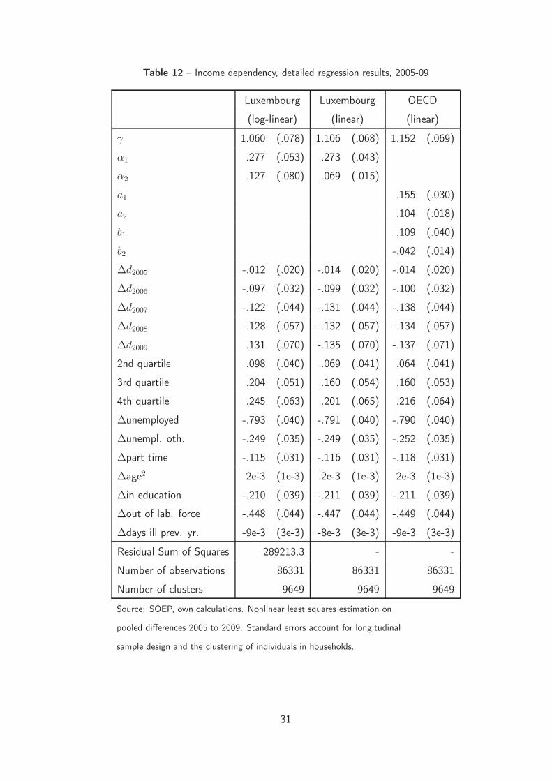
Table 12 – Income dependency, detailed regression results, 2005-09

Luxembourg Luxembourg OECD

(log-linear) (linear) (linear)

γ 1.060 (.078) 1.106 (.068) 1.152 (.069)

α1 .277 (.053) .273 (.043)

α2 .127 (.080) .069 (.015)

a1 .155 (.030)

a2 .104 (.018)

b1 .109 (.040)

b2 -.042 (.014)

∆d2005 -.012 (.020) -.014 (.020) -.014 (.020)

∆d2006 -.097 (.032) -.099 (.032) -.100 (.032)

∆d2007 -.122 (.044) -.131 (.044) -.138 (.044)

∆d2008 -.128 (.057) -.132 (.057) -.134 (.057)

∆d2009 .131 (.070) -.135 (.070) -.137 (.071)

2nd quartile .098 (.040) .069 (.041) .064 (.041)

3rd quartile .204 (.051) .160 (.054) .160 (.053)

4th quartile .245 (.063) .201 (.065) .216 (.064)

∆unemployed -.793 (.040) -.791 (.040) -.790 (.040)

∆unempl. oth. -.249 (.035) -.249 (.035) -.252 (.035)

∆part time -.115 (.031) -.116 (.031) -.118 (.031)

∆age2 2e-3 (1e-3) 2e-3 (1e-3) 2e-3 (1e-3)

∆in education -.210 (.039) -.211 (.039) -.211 (.039)

∆out of lab. force -.448 (.044) -.447 (.044) -.449 (.044)

∆days ill prev. yr. -9e-3 (3e-3) -8e-3 (3e-3) -9e-3 (3e-3)

Residual Sum of Squares 289213.3 - -

Number of observations 86331 86331 86331

Number of clusters 9649 9649 9649




31

Documents

A Goodness-of-Fit Approach to Estimating Equivalence Scalesftp.iza.org/dp7209.pdf · A Goodness-of-Fit Approach to Estimating Equivalence Scales . Martin Biewen . University of Tübingen,