Embed Size (px)
Citation preview
Mathematics Mechanization Research PreprintsKLMM, Chinese Academy of SciencesVol. 29, 189–205, September 2010 189
A Greedy Algorithm for Feed-rate Planning of
CNC Machines along Curved Tool Paths with
Confined Jerk for Each Axis
Ke Zhang, Xiao-Shan Gao, Hongbo Li, Chun-Ming YuanKLMM, Institute of Systems Science, Chinese Academy of Sciences
E-mail: [email protected]
Abstract. The problem of optimal feed-rate planning along a curved tool path for3-axis CNC machines with a jerk limit for each axis is addressed. We prove that theoptimal feed-rate planning must use “Bang-Bang” control, that is, at least one of the axesreaches its jerk bound throughout the motion. As a consequence, the optimal parametricvelocity can be expressed as a piecewise analytic function of the curve parameter u.We also give the explicit formula for the velocity function by solving a second orderdifferential equation. Under a “greedy rule”, an algorithm for optimal jerk confinedfeed-rate planning is presented, together with an example.
Keywords. Optimal feed-rate planning, confined jerk, velocity limit surface, parametrictool path, “Bang-Bang” control.
1 Introduction
The feed-rate optimization along curved tool paths is an important problem in CNC ma-chining. In the feed-rate planning, the acceleration on each axis of the machine must beconstrained, because the torque (or force) capabilities of the axes’ drives are limited. There-fore, the problem is how to identify the feed-rate along a given path such that the machiningtime is minimal without exceeding the capabilities of the actuators.
Bobrow et al [1], Shiller and Lu [2] gave algorithms to determine the minimum-time mo-tion for a robot manipulator along a specific path (at least a smooth curve) with accelerationbounds on x, y, z axes. Farouki and Timar [3, 4] planned the feed-rate for CNC machining,also with acceleration bounds on x, y, z axes, and gave a piecewise-analytic expression ofthe optimal velocity planning function. Yuan and Gao [5] provided a time optimal feed-rateplanning method with tangential acceleration and chord error bounds. All of the methodsmentioned above used the velocity limit curve and its switching points in the u − u phaseplane to obtain an optimal solution which is a continuous time optimal velocity functionalong a specific path. Dong and Stori [6] gave a discrete greedy algorithm for the aboveproblem with a acceleration bound on each axis. These methods are all based on the ideaof “Bang-Bang” control, that is, at least one of the axes reaches its acceleration boundthroughout the motion.
However, the acceleration profile obtained with the above methods has discontinuities,since the acceleration may change from the maximum A to the minimum −A instantly. These
190 K. Zhang et al
discontinuities correspond to step changes in the force output demanded of the drive, causevibrations and then large contouring errors. One method to reduce vibrations is introducingjerk constraints along each axis to the original problem. Then we will obtain a feed-rateplanning with continuous acceleration.
When jerk constraints are added, the analysis must be performed in the u− u− u phasespace instead of the u−u phase plane. The new optimization problem becomes more difficult.However, it is much easier when considering the constraints of the tangential accelerationand jerk. Such problems have received much attention in the robotics and manufacturingliterature. Altintas and Erkorkmaz [8] presented a quintic spline trajectory generation al-gorithm that produces continuous position, velocity, and acceleration profiles with confinedtangential acceleration and jerk. Macfarlane and Croft [9] developed and implemented anonline method to obtain smooth, jerk-bounded trajectories with fifth-order polynomials forindustrial robot applications. Their method is near time optimal with confined tangentialjerk and acceleration. Nam and Yang [10] presented a recursive trajectory generation methodthat estimates an admissible path increment and determines the initiation of the final de-celeration stage according to the distance left to travel estimated at every sampling time,resulting in exact feed-rate trajectory generation through tangential jerk-confined accelera-tion profiles for the parametric curves. Lin et al [11] proposed a dynamics-based interpolatorwith real-time look-ahead algorithm to generate a smooth and tangential jerk-confined ac-celeration/deceleration feed-rate profile. Emami and Arezoo [12] introduced a look-aheadtrajectory generation method which determines the deceleration stage according to the fastestimated arc length and the reverse interpolation of each curve at every sampling time.They obtained a feed-rate trajectory with tangential jerk-confined acceleration profiles forthe NURBS curves. Lai et al [13] further proposed a method which can generate velocitieswith jerk limits as well as chord error, speed, and acceleration limits. The method uses adiscrete model and satisfies all these constraints by backtracking at each step.
In order to make full use of the capabilities of the machine tool, it is desirable to solvethe problem with jerk constraints on each axis, because the drivers of the axes of a CNCmachine are controlled independently. Using a jerk limit on each axis will lead to a continuousacceleration curve for each axis. Dong et al [14] extended their discrete greedy algorithm [6]by adding jerk constraints on each axes and obtained a discrete optimal solution. However,none of these prior approaches have attempted to get an analytical solution with a continuousmodel with jerk constraints on each axis.
In this paper, we consider the problem of optimal feed-rate planning along a specifictool path ~r(u) with a confined jerk on each axis of a 3-axis machine. First, we prove thatthe time-optimal feed-rate planning must use “Bang-Bang” control, that is, at least one ofthe axes reaches its jerk bound throughout the motion. Then we give an optimal feed-rateplanning algorithm under a “greedy rule”: using the maximal jerk as much as possible.
Our algorithm has two key components, which are also the main contribution of thispaper. The first one is how to compute the parametric velocity function after the controlaxis and maximal (or minimal) jerk are given. To compute the parametric velocity function,we need to solve a second-order differential equation, and the analytic solutions are given.We also introduce the CASS (control axis switching surface). The control axis should bechanged when the velocity integration trajectory passes through a CASS. The second key
Algorithm for Feed-rate Planning with Jerk Constraints 191
component is to introduce and use the VLS (velocity limit surface) for the feed-rate planning.It is similar to the VLC (velocity limit curve) in the feed-rate planning with accelerationconstraints [1, 2, 3, 4]. The VLS is a surface in the u − u − u space which limits theparametric velocity and acceleration.
The general idea of our algorithm is to compute the integration trajectory forward from(0, 0, 0) in the u− u− u space under the limit of VLS and our “greedy rule”; then to computethe integration trajectory backward from (1, 0, 0) in a similar way; and finally to obtain acomplete velocity integration trajectory with continuous acceleration by connecting the twointegration trajectories.
The rest of our paper will be organized as follows. Section 2 gives the mathematicaldescription and theoretical analysis of our feed-rate optimization problem. Section 3 givesour feed-rate planning algorithm. Section 4 gives an example. Section 5 concludes the paper.
2 Problem description and theoretical analysis
2.1 Problem description
For brevity, we just consider a plane piecewise parametric curve as the tool path:
~r(u) = (x(u), y(u)), 0 ≤ u ≤ 1,
where x(u), y(u) ∈ C2([0, 1]). Furthermore, we assume that each segment of the curve isinfinitely differentiable. For instance, a cubic B-spline curve satisfies the conditions. Also,we only consider the bounds on the x and y jerk components. The extension to spatial pathsis relatively straightforward but more tedious. We denote the derivatives with respect totime t and the parameter u by dots and primes, respectively:
u = du/dt, x′ = dx/du.
Then, it is obvious that
u′ =u
u, (1)
u′ =...u
u, (2)
and
u′′ = (u
u)′ =
...u
u2− u2
u3. (3)
The jerks on the x and y axes are:{
jx =...x = ((x′u)′u)′u = x′′′u3 + 3x′′u2u′ + x′u(u′)2 + x′u2u′′,
jy =...y = ((y′u)′u)′u = y′′′u3 + 3y′′u2u′ + y′u(u′)2 + y′u2u′′.
(4)
Substituting (1)(3) into (4), jx, jy can be expressed as{
jx = x′′′u3 + 3x′′uu + x′...u ,
jy = y′′′u3 + 3y′′uu + y′...u .(5)
192 K. Zhang et al
We call u, u, and...u parametric velocity, parametric acceleration, and parametric jerk, respec-
tively. Then our feed-rate optimization problem becomes to plan the parametric velocityu ∈ C1([0, 1]), such that the machining time is minimal:
minT =∫ 1
0
du
u(6)
under the following constraints: {|jx| ≤ Jx,
|jy| ≤ Jy,(7)
{u|u=0,1 = 0,
u|u=0,1 = 0,(8)
where Jx, Jy are positive constants, denoting maximal jerks of x, y axes, respectively.
2.2 Optimal solution is “Bang-Bang” control
In this section, we will prove that the solution to our optimal problem must be “Bang-Bang”control, that is, at least one of the axes reaches its jerk bound throughout the motion. Inother words, jx = ±Jx or jy = ±Jy at every time. When there is an axis whose jerk reachesits bound, it is called the control axis.
We prove the claim by contradiction (see Fig.1). Assume that the optimal parametricvelocity function is u, and there exists an interval [u1, u2] in [0, 1], such that neither jx norjy reaches its bound for u ∈ [u1, u2], i.e., the inequalities (7) are strict.
From (4), jx, jy can be expressed as functions in u, u, u′, u′′, denoted by f, g, respectively:{
jx = f(u, u, u′, u′′) = x′′′u3 + 3x′′u2u′ + x′u(u′)2 + x′u2u′′,
jy = g(u, u, u′, u′′) = y′′′u3 + 3y′′u2u′ + y′u(u′)2 + y′u2u′′.
So, for every u ∈ [0, 1], f, g are polynomials in u, u′, u′′. Using (7), there exist positiveconstants A1 and A2, such that
{|f(u, u, u′, u′′)| ≤ A1 < Jx,
|g(u, u, u′, u′′)| ≤ A2 < Jy(9)
is established for u ∈ [u1, u2].For every positive ε, we construct
∆u =
{ε(1 + cos π(2u−u1−u2)
u2−u1) u1 ≤ u ≤ u2;
0 otherwise.
It is easy to show that {∆u|u1,u2 = 0,
(∆u)′|u1,u2 = 0,(10)
Algorithm for Feed-rate Planning with Jerk Constraints 193
Fig. 1. optimal solution is “Bang-Bang” control
and
0 ≤ ∆u ≤ 2ε,
|∆u′| ≤ B1ε,
|∆u′′| ≤ B2ε,
(11)
where B1, B2 are positive constants.Let u∗ = ∆u + u, from (10) we know that u∗ ∈ C1([0, 1]). For every u ∈ [u1, u2], using
first-order Taylor expansion of f, g to u, u′, u′′, we obtain:
f(u, u∗, u∗′, u∗
′′) = f(u, u, u′, u′′) + ∆u
∂f
∂u(u, ξ(u), η(u), τ(u))
+ ∆u′∂f
∂u′(u, ξ(u), η(u), τ(u))
+ ∆u′′∂f
∂u′′(u, ξ(u), η(u), τ(u)),
(12)
where ξ(u) is between u and u∗, η(u) is between u′ and u∗′ , and τ(u) is between u′′ and u∗′′ .So ξ(u), η(u), τ(u) are bounded for u ∈ [u1, u2]. Because the partial derivatives of f in (12)are all polynomials in u, u′, u′′, we have constants F1, F2, F3 such that ∀u ∈ [u1, u2]:
|∂f
∂u(u, ξ(u), η(u), τ(u))| ≤ F1,
| ∂f
∂u′(u, ξ(u), η(u), τ(u))| ≤ F2,
| ∂f
∂u′′(u, ξ(u), η(u), τ(u))| ≤ F3.
(13)
Using (9) (11) (12) (13), we have:
|f(u, u∗, u∗′, u∗
′′)| ≤ A1 + C1ε,
where C1 = 2F1 + B1F2 + B2F3. In a similar way, there exists a C2 such that:
|g(u, u∗, u∗′, u∗
′′)| ≤ A2 + C2ε.
194 K. Zhang et al
We just need to choose
ε = min{(Jx −A1)/C1, (Jy −A2)/C2},
and then u∗ also satisfies the constraints (7) (8) and the continuity condition. But we haveu∗ ≥ u, and u∗ > u for u ∈ (u1, u2), from (6) we know that u∗ is a better solution, whichcontradicts the original claim of optimality of u. So the optimal solution of our problem is“Bang-Bang” control.
3 Feed-rate planning algorithm
The key idea of our algorithm for feed-rate optimization along curved tool paths is: in theu − u − u space, using the jerk constraints to deduce a kind of velocity limit surfaces, thengenerating an integration trajectory with the maximal parametric jerk under the limit ofsuch kind of surfaces. Before the integration trajectory reaches these surfaces, we use theminimal parametric jerk to generate an integration trajectory to keep the continuity of theacceleration curve.
3.1 Parametric jerk constraints
Using (5) (7), we can rewrite the jerk limits to be constraints of the parametric jerk...u :
(a) When x′y′ 6= 0, (7) is equivalent to:{
f1(u, u, u) ≤ ...u ≤ g1(u, u, u),
f2(u, u, u) ≤ ...u ≤ g2(u, u, u),
(14)
where
f1(u, u, u) ={
(−Jx − x′′′u3 − 3x′′uu)/x′ x′ > 0;(Jx − x′′′u3 − 3x′′uu)/x′ x′ < 0.
g1(u, u, u) ={
(Jx − x′′′u3 − 3x′′uu)/x′ x′ > 0;(−Jx − x′′′u3 − 3x′′uu)/x′ x′ < 0.
f2(u, u, u) ={
(−Jy − y′′′u3 − 3y′′uu)/y′ y′ > 0;(Jy − y′′′u3 − 3y′′uu)/y′ y′ < 0.
g2(u, u, u) ={
(Jy − y′′′u3 − 3y′′uu)/y′ y′ > 0;(−Jy − y′′′u3 − 3y′′uu)/y′ y′ < 0.
Let {J−(u, u, u) = max{f1, f2},J+(u, u, u) = min{g1, g2}.
(15)
Then constraints (14) become
J−(u, u, u) ≤ ...u ≤ J+(u, u, u). (16)
It shows that in every point of the u− u− u space,...u has upper and lower bounds: J+, J−.
Algorithm for Feed-rate Planning with Jerk Constraints 195
(b) When x′ = 0, (7) becomes:{−Jx ≤ x′′′u3 + 3x′′uu ≤ Jx,
f2(u, u, u) ≤ ...u ≤ g2(u, u, u).
(17)
The first equation of (17) indicates the range of (u, u) on the u section where u satisfies x′ = 0.The range is limited by two curves x′′′u3+3x′′uu = −Jx and x′′′u3+3x′′uu = Jx in the u−u−uspace. We call these curves type one velocity switching curve (abbr. VSC1). The secondequation of (17) still shows the upper and lower bounds of
...u , where now J+ = g2, J− = f2.
(c) When y′ = 0, the analysis to the following equations are similar:{
f1(u, u, u) ≤ ...u ≤ g1(u, u, u),
−Jy ≤ y′′′u3 + 3y′′uu ≤ Jy.(18)
The first equation of (18) shows the upper and lower bounds of...u , where J+ = g1, J− = f1.
The second equation of (18) indicates the range of (u, u) on the u section where u satisfiesy′ = 0. It is limited by two curves y′′′u3 + 3y′′uu = −Jy and y′′′u3 + 3y′′uu = Jy in theu− u− u space. These curves are also VSC1.
3.2 Integration trajectory and control axis switching surface
Since we have proven that the solution to our optimal problem uses“Bang-Bang” control,it is necessary to deduce the parametric velocity function u when any axis reaches its jerkbound. Using (1), it is easy to show that once the parametric velocity function u in u isknown, the parametric acceleration function u in u is determined. Then the two functions uand u in u determine a curve in the u− u− u space. We call the curve integration trajectory.This subsection will discuss 1) how to compute the parametric velocity function when anyaxis reaches its jerk bound and 2) how to choose control axis and switch axis.
Firstly, we deal with the solutions of parametric velocity function u. For example, ifthe x-axis reaches its jerk bound Jx, we need to solve the following second-order differentialequation:
((x′u)′u)′u = Jx. (19)
Let f = x′u. The differential equation becomes
d
dx(df
dxf)f = Jx.
Let g = dfdx . Then we have
g2f + gf2 dg
df= Jx.
Let h = g2. The equation above becomes
dh
df=
2Jx
f2− 2h
f.
196 K. Zhang et al
Solving the differential equation, we obtain
h =2Jx
f− C1
f2, (20)
where C1 is an integration constant. The above equation can be rewritten as
df
dx= ±
√2Jxf − C1
f.
We solve it to obtain
x− C2 = ±∫
fdf√2Jxf − C1
= ±(C1
√2Jxf − C1 +
13
√2Jxf − C1
3)/2J2
x , (21)
where C2 is an integration constant. We solve the equation above to obtain
u =1
2Jxx′[ω(U +
√U2 + C3
1 )23 + ω2(U −
√U2 + C3
1 )23 − C1], (22)
where U = 3J2x(x− C2), ω3 = 1.
Now we deduce the expressions of these integration constants C1, C2 in u, u, u for ourlater algorithm. We have
h = (df
dx)2 = (
x′′u2 + x′ux′u
)2.
Substituting it into (20), we get
C1 = 2Jxf − hf2 = 2Jxx′u− (x′′u2 + x′u)2. (23)
Use (21) (23) to obtain
C2 = x± ((x′′u2 + x′u)3 − 3Jxx′u(x′′u2 + x′u))/3J2x . (24)
Then from (23) (24), the integration constants C1, C2 are determined by specifying a knownpoint on the integration trajectory in the u− u− u space.
If y-axis reaches its jerk bound Jy, we solve the parametric velocity function in the sameway to get
u =1
2Jyy′[ω(U +
√U2 + C3
1 )23 + ω2(U −
√U2 + C3
1 )23 − C1], (25)
where U = 3J2y (y − C2), ω3 = 1. We also have
C1 = 2Jyy′u− (y′′u2 + y′u)2, (26)
C2 = y ± ((y′′u2 + y′u)3 − 3Jyy′u(y′′u2 + y′u))/3J2
y . (27)
Algorithm for Feed-rate Planning with Jerk Constraints 197
In (22) or (25), if U2 +C31 is negative in some interval of u, the expression of u should be
converted, for the convenience of our computation. Taking (25) for example, we substituteω by e
23ikπ (k = 0, 1, 2) to obtain
u =−C1
2Jyy′[e
23ikπ(
U
(−C1)3/2+ i
√1− U2
(−C1)3)2/3 + e−
23ikπ(
U
(−C1)3/2− i
√1− U2
(−C1)3)2/3 + 1]
=−C1
2Jyy′[e
23ikπe
23i arccos U
(−C1)3/2 + e−23ikπe
− 23i arccos U
(−C1)3/2 + 1]
=−C1
2Jyy′[2 cos
23(arccos
U
(−C1)3/2+ kπ) + 1].
If x (or y)-axis reaches its jerk bound −Jx (or −Jy), we just need to replace Jx (or Jy)by −Jx (or −Jy) in the solutions above.
Now we turn to deal with how to decide the control axis. There are two problems:determining control axis at the starting point and axis switching during the motion.
If we integrate...u = J+(u, u, u) forward from (0, 0, 0) in the u− u− u space as the current
integration trajectory, it is easy to determine the control axis from (u, u, u) = (0, 0, 0) andthe three cases (a),(b),(c) in section 3.1. For example, when x′(0) > 0, y′(0) > 0, x-axis isthe control axis if and only if g1(0, 0, 0) = Jx/x′ < g2(0, 0, 0) = Jy/y′.
From (15), when we integrate...u = J+(u, u, u), the expression of the parametric velocity
may change if the values of g1, g2 vary. It means that the control axis should be switched.So we call g1 = g2 the control axis switching surface (abbr. CASS). For example, if theintegration trajectory passes through a CASS from the region g1 < g2 to the region g1 > g2,the control axis should be switched from x to y, and vice versa.
The situation is similar when integrating...u = J−(u, u, u), and the CASS is then f1 = f2.
When the integration trajectory passes through the CASS from the region f1 > f2 to theregion f1 < f2, the control axis should be switched from x to y, and vice versa. We willnot mention about how to deal with the CASS when integrating
...u = J+(u, u, u) or
...u =
J−(u, u, u) in our later algorithm.
3.3 Velocity limit surface and velocity switching curve
Let J−(u, u, u) and J+(u, u, u) be the expressions defined in (15). We call J−(u, u, u) =J+(u, u, u) the velocity limit surface (abbr. VLS), which is an algebraic surface in the fol-lowing region of the u− u− u space:
D = {(u, u, u)|0 ≤ u ≤ 1, u ≥ 0}.
Obviously, the integration trajectories cannot go beyond the VLS, that is, we can only planthe integration trajectories in the region where J−(u, u, u) ≤ J+(u, u, u) is valid. Intuitively,this region is just a part of D divided by the VLS, which contains (0, 0, 0), (1, 0, 0) (see Fig.2).
From f1 < g1, f2 < g2, and (14) (15), we know that the VLS has two components:
f1(u, u, u) = g2(u, u, u),
198 K. Zhang et al
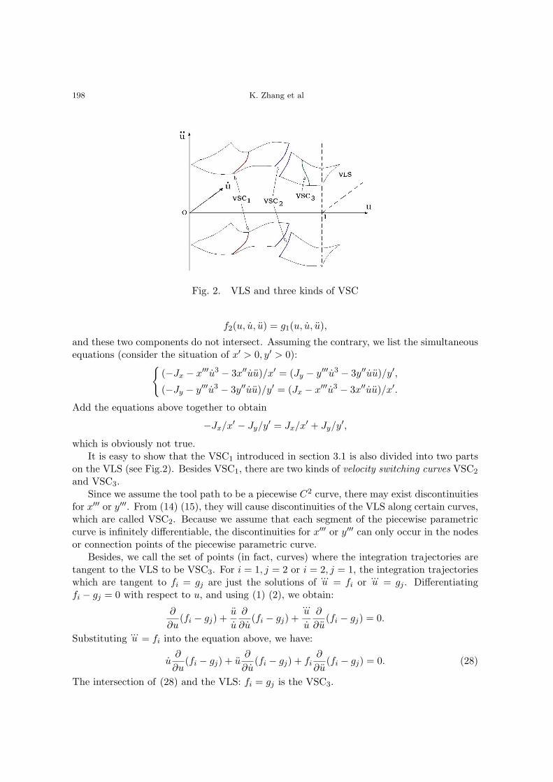
Fig. 2. VLS and three kinds of VSC
f2(u, u, u) = g1(u, u, u),
and these two components do not intersect. Assuming the contrary, we list the simultaneousequations (consider the situation of x′ > 0, y′ > 0):
{(−Jx − x′′′u3 − 3x′′uu)/x′ = (Jy − y′′′u3 − 3y′′uu)/y′,
(−Jy − y′′′u3 − 3y′′uu)/y′ = (Jx − x′′′u3 − 3x′′uu)/x′.
Add the equations above together to obtain
−Jx/x′ − Jy/y′ = Jx/x′ + Jy/y′,
which is obviously not true.It is easy to show that the VSC1 introduced in section 3.1 is also divided into two parts
on the VLS (see Fig.2). Besides VSC1, there are two kinds of velocity switching curves VSC2
and VSC3.Since we assume the tool path to be a piecewise C2 curve, there may exist discontinuities
for x′′′ or y′′′. From (14) (15), they will cause discontinuities of the VLS along certain curves,which are called VSC2. Because we assume that each segment of the piecewise parametriccurve is infinitely differentiable, the discontinuities for x′′′ or y′′′ can only occur in the nodesor connection points of the piecewise parametric curve.
Besides, we call the set of points (in fact, curves) where the integration trajectories aretangent to the VLS to be VSC3. For i = 1, j = 2 or i = 2, j = 1, the integration trajectorieswhich are tangent to fi = gj are just the solutions of
...u = fi or
...u = gj . Differentiating
fi − gj = 0 with respect to u, and using (1) (2), we obtain:
∂
∂u(fi − gj) +
u
u
∂
∂u(fi − gj) +
...u
u
∂
∂u(fi − gj) = 0.
Substituting...u = fi into the equation above, we have:
u∂
∂u(fi − gj) + u
∂
∂u(fi − gj) + fi
∂
∂u(fi − gj) = 0. (28)
The intersection of (28) and the VLS: fi = gj is the VSC3.
Algorithm for Feed-rate Planning with Jerk Constraints 199
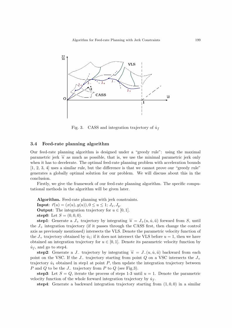
Fig. 3. CASS and integration trajectory of uf
3.4 Feed-rate planning algorithm
Our feed-rate planning algorithm is designed under a “greedy rule”: using the maximalparametric jerk
...u as much as possible, that is, we use the minimal parametric jerk only
when it has to decelerate. The optimal feed-rate planning problem with acceleration bounds[1, 2, 3, 4] uses a similar rule, but the difference is that we cannot prove our “greedy rule”generates a globally optimal solution for our problem. We will discuss about this in theconclusion.
Firstly, we give the framework of our feed-rate planning algorithm. The specific compu-tational methods in the algorithm will be given later.
Algorithm. Feed-rate planning with jerk constraints.Input: ~r(u) = (x(u), y(u)), 0 ≤ u ≤ 1; Jx, Jy.Output: The integration trajectory for u ∈ [0, 1].step0: Let S = (0, 0, 0).step1: Generate a J+ trajectory by integrating
...u = J+(u, u, u) forward from S, until
the J+ integration trajectory (if it passes through the CASS first, then change the controlaxis as previously mentioned) intersects the VLS. Denote the parametric velocity function ofthe J+ trajectory obtained by u1; if it does not intersect the VLS before u = 1, then we haveobtained an integration trajectory for u ∈ [0, 1]. Denote its parametric velocity function byuf , and go to step4.
step2: Generate a J− trajectory by integrating...u = J−(u, u, u) backward from each
point on the VSC. If the J− trajectory starting from point Q on a VSC intersects the J+
trajectory u1 obtained in step1 at point P , then update the integration trajectory betweenP and Q to be the J− trajectory from P to Q (see Fig.3).
step3: Let S = Q, iterate the process of steps 1-3 until u = 1. Denote the parametricvelocity function of the whole forward integration trajectory by uf .
step4: Generate a backward integration trajectory starting from (1, 0, 0) in a similar
200 K. Zhang et al
way as step1-step3 until u = 0. Denote the parametric velocity function of the backwardintegration trajectory by ub.
step5: Connect the two integration trajectories of uf and ub by J− trajectories. Weobtain a complete integration trajectory for u ∈ [0, 1].
Remark. The “greedy” rule is used in step 2. In step 1, the J+ integration trajectoryu1 meets the VLS at a point. If we continue to use the same jerk, u1 will pass through theVLS and violate the jerk limits. In other words, we must decelerate before this happens.According to the definition, the integration trajectory can meet the VSC at a point in aVSC. That is why we generate a J− integration trajectory starting from a point in the nextVSC and try to use this trajectory as the decelerate part of the whole trajectory. In otherwords, we use the maximal parametric jerk to accelerate as long as possible and then usethe minimal parametric jerk to decelerate so that the jerk limits (VLS) are not violated.
Concrete computational methods of step2 and step5 in our algorithm are given below.We will treat step5 first.
For step5, because the control axes of the forward and backward integration trajectoriesmay have been switched for several times, uf and ub are both piecewise-analytic functions (seeFig.3). We need to traverse and choose each analytic segment of the forward and backwardintegration trajectories respectively, and to connect these two segments by a J− trajectoryif there exists such a solution (if we connect them by a J+ trajectory, the two segmentswhich are connected can only be J− trajectories, this will violate our “greedy rule”). Afterchoosing one segment in uf and ub respectively, there are two cases:
1) The J− trajectory for connection does not pass through CASS. Assume the J− trajec-tory starts from point (u1, uf (u1), uf (u1)) on the forward trajectory to point (u2, ub(u2), ub(u2))on the backward trajectory in the u−u−u space. From (23) (24) or (26) (27), the integrationconstants of the J− trajectory can be expressed as C1(u, u, u), C2(u, u, u). We need to solvethe following algebraic equation system
{C1(u1, uf (u1), uf (u1)) = C1(u2, ub(u2), ub(u2)),C2(u1, uf (u1), uf (u1)) = C2(u2, ub(u2), ub(u2))
(29)
to obtain u1, u2. Then the integration constants of the J− connection trajectory are C1(u1,uf (u1), uf (u1)), C2(u1, uf (u1), uf (u1)), where u1 is a solution of equation (29). Then weobtain the J− trajectory for the connection in step5.
2) The J− trajectory for connection passes through an CASS. Now the expressions ofthe J− trajectory and its integration constants are different in the two sides of the CASS.Suppose the left side is controlled by jx = −Jx and the right side is controlled by jy = −Jy.Denote the integration constants of the jx = −Jx trajectory by Cx
1 , Cx2 and the integration
constants of jy = −Jy trajectory by Cy1 , Cy
2 . Assume the J− trajectory for connection passesthrough the CASS at the point (uc, uc, uc), and it starts from the point (ul, uf (ul), uf (ul))on the forward trajectory to the point (ur, ub(ur), ub(ur)) on the backward trajectory. Then,
Algorithm for Feed-rate Planning with Jerk Constraints 201
we need to solve the following algebraic equation system
f1(uc, uc, uc) = f2(uc, uc, uc),Cx
1 (ul, uf (ul), uf (ul)) = Cx1 (uc, uc, uc),
Cx2 (ul, uf (ul), uf (ul)) = Cx
2 (uc, uc, uc),Cy
1 (ur, ub(ur), ub(ur)) = Cy1 (uc, uc, uc),
Cy2 (ur, ub(ur), ub(ur)) = Cy
2 (uc, uc, uc)
(30)
to obtain ul, uc, ur, uc, uc and the two sets of integration constants of the J− trajectory forthe connection: Cx
1 (uc, uc, uc), Cx2 (uc, uc, uc) and Cy
1 (uc, uc, uc), Cy2 (uc, uc, uc). It is similar
to deal with the case when the J− trajectory passes through the CASS more than once.In general, the solutions of the above equation systems are finite. We just need to compare
these solutions to get an optimal one according to the machining time in (6).For step2, there are two cases:1) Point Q is on a VSC1 or a VSC2. If u = u0 at Q, we assume the coordinate of Q
is (u, u, u) = (u0, b, c) and denote the expression of VSC1 or VSC2 on the u0 section byh1(u, u) = 0 as previously mentioned. Assume u = a at P . Then the coordinate of P is(a, u1(a), u1(a)). The integration constants of the J− trajectory are C1(u, u, u), C2(u, u, u)as above. We just need to solve the following algebraic equation system
C1(u0, b, c) = C1(a, u1(a), u1(a)),C2(u0, b, c) = C2(a, u1(a), u1(a)),
h1(b, c) = 0(31)
to obtain a, b, c. If the equation system has more than one solutions or there are more VSCs,we should choose the solution with maximal parametric a according to our “greedy rule” .We deal with equation systems occurring later in the same way. The integration constantsof the J− trajectory can be computed by C1(u0, b, c), C2(u0, b, c). Then we obtain the J−trajectory in step2.
2) Point Q is on a VSC3. Assume the coordinate of Q to be (d0, b0, c0). From (28),denote the VSC3 by {(u, u, u)|h2(u, u, u) = 0, h3(u, u, u) = 0}. Assume u = a0 at P . Thenthe coordinate of P is (a0, u1(a0), u1(a0)). The integration constants of the J− trajectory canalso be expressed as C1(u, u, u) and C2(u, u, u). We just need to solve the following algebraicequation system
C1(d0, b0, c0) = C1(a0, u1(a0), u1(a0)),C2(d0, b0, c0) = C2(a0, u1(a0), u1(a0)),h2(d0, b0, c0) = 0,
h3(d0, b0, c0) = 0
(32)
to obtain a0, d0, b0, c0. The integration constants of the J− trajectory are C1(d0, b0, c0) andC2(d0, b0, c0). If the J− trajectory passes through a CASS between P and Q, we use themethod mentioned above for case 2) of step5 to deal with this situation.
So far, we have obtained a complete integration trajectory, its parametric velocity func-tion satisfies (7) (8) and our “greedy rule”.
With the algorithm, we obviously obtain a unique and optimal feed-rate planning alongspecific tool paths with jerk constraints on each axis under the “greedy rule”.
202 K. Zhang et al
1.00.75
0.5-20.0
du/dt
-1
uuu
0.25
0
u
1
0.50.25
2
0.75 1.00.0
1.00.75
0.5-20.0
du/dt
-1
uuu
0.25
0
u
1
0.50.25
2
0.75 1.00.0
1.00.75
0.5-20.0
du/dt
-1
uuu
0.25
0
1
u
0.50.25
2
0.75 1.00.0
(a) VLS (b) CASS (c) CASS
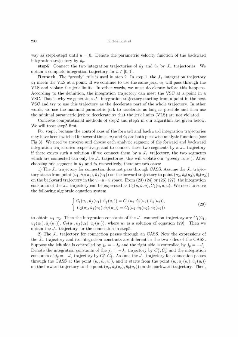
Fig. 4. VLS and CASS
1.00.75
0.5-20.0
uu
-1
uuu
0.25
0
1
u
0.50.25
2
0.75 1.00.0
1.00.75
0.5 uu0.25
0.0-2
0.25
u
0.5
-1
0.75 1.0
uuu 0
0.0
1
2
1.00.75
0.5 uu0.25
0.0-2
0.25
u
0.5
-1
0.75 1.0
uuu
0.0
0
1
2
(a) (b) (c)
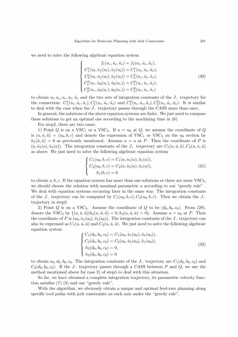
Fig. 5. Forward integration trajectory: (a); backward integration trajectory: (b) and (c)
4 An example
We use the following example to illustrate our algorithm:
~r(u) = (u, u2), 0 ≤ u ≤ 1,
Jx = Jy = 1.
The algorithm has the following steps:1) Firstly, compute the VLS and the CASS :
Fig.4(a): VLS J−(u, u, u) = J+(u, u, u);Fig.4(b): CASS of maximal parametric jerk g1(u, u, u) = g2(u, u, u);Fig.4(c): CASS of minimal parametric jerk f1(u, u, u) = f2(u, u, u).
Then, compute the three kinds of VSC :VSC1: {(0, u, u) | 1− 6uu = 0} and {(0, u, u) | 1 + 6uu = 0};VSC3: {(u, u, u) | 1−6uu+2u = 0, 4u−3u2 = 0} and {(u, u, u) | 1+6uu+2u = 0, 4u+3u2 =0};VSC2 dose not exist here.
2) Generate a J+ trajectory forward from (0, 0, 0). The trajectory is controlled by jx = Jx
in the beginning, then intersects the CASS g1 = g2 at u = 0.05 and switches to the controlof jy = Jy. It will not intersect the VLS or the CASS before reaching u = 1 (Fig.5(a)). We
Algorithm for Feed-rate Planning with Jerk Constraints 203
1.00.750.5 uu
0.25
0.0
-2
0.25
u
-1
0.5
uuu 0
0.75 1.0
1
0.0
2
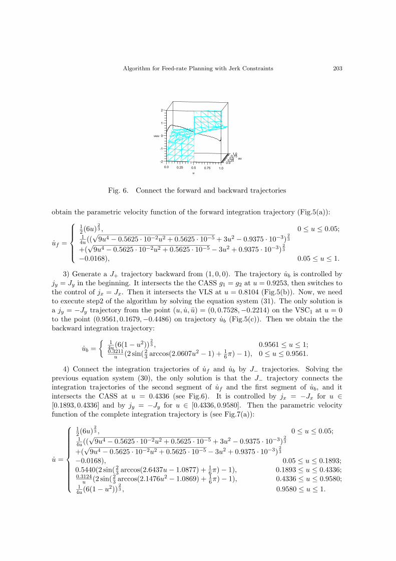
Fig. 6. Connect the forward and backward trajectories
obtain the parametric velocity function of the forward integration trajectory (Fig.5(a)):
uf =
12(6u)
23 , 0 ≤ u ≤ 0.05;
14u((
√9u4 − 0.5625 · 10−2u2 + 0.5625 · 10−5 + 3u2 − 0.9375 · 10−3)
23
+(√
9u4 − 0.5625 · 10−2u2 + 0.5625 · 10−5 − 3u2 + 0.9375 · 10−3)23
−0.0168), 0.05 ≤ u ≤ 1.
3) Generate a J+ trajectory backward from (1, 0, 0). The trajectory ub is controlled byjy = Jy in the beginning. It intersects the the CASS g1 = g2 at u = 0.9253, then switches tothe control of jx = Jx. Then it intersects the VLS at u = 0.8104 (Fig.5(b)). Now, we needto execute step2 of the algorithm by solving the equation system (31). The only solution isa jy = −Jy trajectory from the point (u, u, u) = (0, 0.7528,−0.2214) on the VSC1 at u = 0to the point (0.9561, 0.1679,−0.4486) on trajectory ub (Fig.5(c)). Then we obtain the thebackward integration trajectory:
ub ={
14u(6(1− u2))
23 , 0.9561 ≤ u ≤ 1;
0.3211u (2 sin(2
3 arccos(2.0607u2 − 1) + 16π)− 1), 0 ≤ u ≤ 0.9561.
4) Connect the integration trajectories of uf and ub by J− trajectories. Solving theprevious equation system (30), the only solution is that the J− trajectory connects theintegration trajectories of the second segment of uf and the first segment of ub, and itintersects the CASS at u = 0.4336 (see Fig.6). It is controlled by jx = −Jx for u ∈[0.1893, 0.4336] and by jy = −Jy for u ∈ [0.4336, 0.9580]. Then the parametric velocityfunction of the complete integration trajectory is (see Fig.7(a)):
u =
12(6u)
23 , 0 ≤ u ≤ 0.05;
14u((
√9u4 − 0.5625 · 10−2u2 + 0.5625 · 10−5 + 3u2 − 0.9375 · 10−3)
23
+(√
9u4 − 0.5625 · 10−2u2 + 0.5625 · 10−5 − 3u2 + 0.9375 · 10−3)23
−0.0168), 0.05 ≤ u ≤ 0.1893;0.5440(2 sin(2
3 arccos(2.6437u− 1.0877) + 16π)− 1), 0.1893 ≤ u ≤ 0.4336;
0.3124u (2 sin(2
3 arccos(2.1476u2 − 1.0869) + 16π)− 1), 0.4336 ≤ u ≤ 0.9580;
14u(6(1− u2))
23 , 0.9580 ≤ u ≤ 1.
204 K. Zhang et al
u0 0.2 0.4 0.6 0.8 1.0
0
0.1
0.2
0.3
0.4
0.5
u0.2 0.4 0.6 0.8 1.0
K0.4
K0.2
0
0.2
0.4
0.6
u0.2 0.4 0.6 0.8 1.0
K1.0
K0.5
0
0.5
1.0
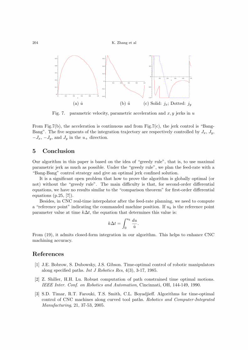
(a) u (b) u (c) Solid: jx; Dotted: jy
Fig. 7. parametric velocity, parametric acceleration and x, y jerks in u
From Fig.7(b), the acceleration is continuous and from Fig.7(c), the jerk control is “Bang-Bang”. The five segments of the integration trajectory are respectively controlled by Jx, Jy,−Jx, −Jy, and Jy in the u+ direction.
5 Conclusion
Our algorithm in this paper is based on the idea of “greedy rule”, that is, to use maximalparametric jerk as much as possible. Under the “greedy rule”, we plan the feed-rate with a“Bang-Bang” control strategy and give an optimal jerk confined solution.
It is a significant open problem that how to prove the algorithm is globally optimal (ornot) without the “greedy rule”. The main difficulty is that, for second-order differentialequations, we have no results similar to the “comparison theorem” for first-order differentialequations (p.25, [7]).
Besides, in CNC real-time interpolator after the feed-rate planning, we need to computea “reference point” indicating the commanded machine position. If uk is the reference pointparameter value at time k∆t, the equation that determines this value is:
k∆t =∫ uk
0
du
u.
From (19), it admits closed-form integration in our algorithm. This helps to enhance CNCmachining accuracy.
References
[1] J.E. Bobrow, S. Dubowsky, J.S. Gibson. Time-optimal control of robotic manipulatorsalong specified paths. Int J Robotics Res, 4(3), 3-17, 1985.
[2] Z. Shiller, H.H. Lu. Robust computation of path constrained time optimal motions.IEEE Inter. Conf. on Robotics and Automation, Cincinnati, OH, 144-149, 1990.
[3] S.D. Timar, R.T. Farouki, T.S. Smith, C.L. Boyadjieff. Algorithms for time-optimalcontrol of CNC machines along curved tool paths. Robotics and Computer-IntegratedManufacturing, 21, 37-53, 2005.
Algorithm for Feed-rate Planning with Jerk Constraints 205
[4] S.D. Timar, R.T. Farouki. Time-optimal traversal of curved paths by Cartesian CNCmachines under both constant and speed-dependent axis acceleration bounds. Roboticsand Computer-Integrated Manufacturing, 23(2), 563-579, 2007.
[5] C.M. Yuan, X.S. Gao. Time-optimal interpolation of CNC machines along parametricpath with chord error and tangential acceleration bounds. MM-preprints, 29, 165-188,2010.
[6] J. Dong, J.A. Stori. A generalized time-optimal bi-directional scan algorithm for con-strained feedrate optimization. ASME Journal of Dynamic Systems, Measurement, andControl, 128, 379-390, 2006.
[7] G. Birkhoff, G.C. Rota. Ordinary differential equations. John Wiley, New York, 1969.
[8] K. Erkorkmaz, Y. Altintas. High speed CNC system design Part I: jerk limited trajectorygeneration and quintic spline interpolation. International Journal of Machine Tools andManufacture, 41, 1323-1345, 2001.
[9] S. Macfarlane, E.A. Croft. Jerk-bounded manipulator trajectory planning: design forreal-time applications. IEEE Transactions on Robotics and Automation. 19, 42-52, 2003.
[10] S.H. Nam, M.Y. Yang. A study on a generalized parametric interpolator with real-timejerklimited acceleration. Computer-Aided Design, 36, 27-36, 2004.
[11] M.T. Lin, M.S. Tsai, H.T. Yau. Development of a dynamics-based NURBS interpola-tor with real-time look-ahead algorithm. International Journal of Machine Tools andManufacture, 47(15), 2246-2262, 2007.
[12] M.M. Emami, B. Arezoo. A look-ahead command generator with control over trajectoryand chord error for NURBS curve with unknown arc length. Computer-Aided Design,42, 625-632, 2010.
[13] J.Y. Lai, K.Y. Lin, S.J. Tseng, W.D. Ueng. On the development of a parametric in-terpolator with confined chord error, feedrate, acceleration and jerk Int J Adv ManufTechnol, 37(1-2), 104-121,2008
[14] J. Dong, P.M. Ferreiraa, J.A. Stori. Feed-rate optimization with jerk constraints for gen-erating minimum-time trajectories. International Journal of Machine Tools and Manu-facture, 47, 1941-1955, 2007.