Office of Research and DevelopmentNational Risk Management Research Laboratory, Ada, Oklahoma 74820

A Guide for Assessing Biodegradation and Source Identification of Organic Ground Water Contaminants using Compound Specific Isotope Analysis (CSIA)

EPA 600/R-08/148 | December 2008 | www.epa.gov/ada

Office of Research and DevelopmentNational Risk Management Research Laboratory, Ada, Oklahoma 74820

Office of Research and DevelopmentNational Risk Management Research Laboratory, Ada, Oklahoma 74820

A Guide for Assessing Biodegradation and Source Identification of Organic Ground Water Contaminants using Compound Specific Isotope Analysis (CSIA)

Daniel HunkelerUniversity of Neuchâtel, Center of Hydrogeology, Neuchâtel, Switzerland

Rainer U. MeckenstockInstitute of Groundwater Ecology, Neuherberg, Germany

Barbara Sherwood LollarUniversity of Toronto, Ontario, Canada

Torsten C. SchmidtUniversity of Duisburg-Essen, Duisburg, Germany

John T. WilsonNational Risk Management Research Laboratory, U.S. Environmental Protection Agency, Ada, Oklahoma, USA

ii

Notice The International Atomic Energy Agency, and the U.S. Environmental Protection Agency through

its Office of Research and Development, funded and managed the development of this Guide. It has been subjected to U.S. Environmental Protection Agency peer and administrative review and has been approved for publication as an EPA document. Mention of trade names or commercial products does not constitute endorsement or recommendation for use.

All research projects making conclusions or recommendations based on environmental data and funded by the U.S. Environmental Protection Agency are required to participate in the Agency Quality Assurance Program. This project did not involve the collection and use of environmental data and, as such, did not require a Quality Assurance Plan.

Front Cover photos:

#1 an isotope ratio mass spectrometer

#2 purging a well to provide a sample of ground water for analysis

iii

Foreword

The U.S. Environmental Protection Agency is charged by Congress with protecting the Nation’s land, air, and water resources. Under a mandate of national environmental laws, the Agency strives to formulate and implement actions leading to a compatible balance between human activities and the ability of natural systems to support and nurture life. To meet this mandate, EPA’s research program is providing data and technical support for solving environmental problems today and building a science knowledge base necessary to manage our ecological resources wisely, understand how pollutants affect our health, and prevent or reduce environmental risks in the future.The National Risk Management Research Laboratory is the Agency’s center for investigation of technological and management approaches for preventing and reducing risks from pollution that threatens human health and the environment. The focus of the Laboratory’s research program is on methods and their cost-effectiveness for prevention and control of pollution to air, land, water, and subsurface resources; protection of water quality in public water systems; remediation of contaminated sites, sediments and ground water; prevention and control of indoor air pollution; and restoration of ecosystems. NRMRL collaborates with both public and private sector partners to foster technologies that reduce the cost of compliance and to anticipate emerging problems. NRMRL’s research provides solutions to environmental problems by: developing and promoting technologies that protect and improve the environment; advancing scientific and engineering information to support regulatory and policy decisions; and providing the technical support and information transfer to ensure implementation of environmental regulations and strategies at the national, state, and community levels.As part of the U.S. EPA Quality System for Environmental Data and Technology, U.S. EPA requires that a Quality Assurance Project Plan (QAPP) be developed and approved before environmental samples are collected and analyzed. Compound Specific Isotope Analysis (CSIA) has only recently been applied to understand the degradation of organic compounds, or to identify the sources of ground water contamination at hazardous waste sites. As a result, there is little information available that can be used to develop, review, or approve a QAPP for the application of CSIA at a hazardous waste site. This Guide provides general recommendations on good practice for sampling ground water for CSIA, and quality assurance recommendations for measurement of isotope ratios. The Guide also provides recommendations for data evaluation and interpretation to use CSIA to document degradation of organic contaminants, or to associate plumes of contaminants in ground water with their sources.

Robert W. Puls, Acting Director

Ground Water and Ecosystems Restoration Division National Risk Management Research Laboratory

v

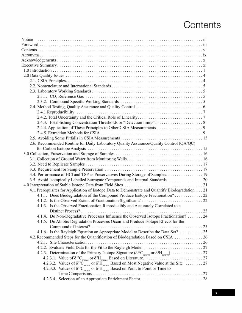
ContentsNotice . . . . . . . . . . . . . . . . . . . . . . . . . . . . . . . . . . . . . . . . . . . . . . . . . . . . . . . . . . . . . . . . . . . . . . . . . . . . . iiForeword . . . . . . . . . . . . . . . . . . . . . . . . . . . . . . . . . . . . . . . . . . . . . . . . . . . . . . . . . . . . . . . . . . . . . . . . . . . iiiContents . . . . . . . . . . . . . . . . . . . . . . . . . . . . . . . . . . . . . . . . . . . . . . . . . . . . . . . . . . . . . . . . . . . . . . . . . . . . vAcronyms. . . . . . . . . . . . . . . . . . . . . . . . . . . . . . . . . . . . . . . . . . . . . . . . . . . . . . . . . . . . . . . . . . . . . . . . . . . ixAcknowledgements . . . . . . . . . . . . . . . . . . . . . . . . . . . . . . . . . . . . . . . . . . . . . . . . . . . . . . . . . . . . . . . . . . . xExecutive Summary . . . . . . . . . . . . . . . . . . . . . . . . . . . . . . . . . . . . . . . . . . . . . . . . . . . . . . . . . . . . . . . . . . . xi 1.0 Introduction . . . . . . . . . . . . . . . . . . . . . . . . . . . . . . . . . . . . . . . . . . . . . . . . . . . . . . . . . . . . . . . . . . . . . 1 2.0 Data Quality Issues . . . . . . . . . . . . . . . . . . . . . . . . . . . . . . . . . . . . . . . . . . . . . . . . . . . . . . . . . . . . . . . 4

2.1. CSIA Principles. . . . . . . . . . . . . . . . . . . . . . . . . . . . . . . . . . . . . . . . . . . . . . . . . . . . . . . . . . . . . . . 42.2. Nomenclature and International Standards . . . . . . . . . . . . . . . . . . . . . . . . . . . . . . . . . . . . . . . . . . 52.3. Laboratory Working Standards . . . . . . . . . . . . . . . . . . . . . . . . . . . . . . . . . . . . . . . . . . . . . . . . . . . 5

2.3.1. CO2 Reference Gas . . . . . . . . . . . . . . . . . . . . . . . . . . . . . . . . . . . . . . . . . . . . . . . . . . . . . . 52.3.2. Compound Specific Working Standards . . . . . . . . . . . . . . . . . . . . . . . . . . . . . . . . . . . . . . 5

2.4. Method Testing, Quality Assurance and Quality Control . . . . . . . . . . . . . . . . . . . . . . . . . . . . . . . 62.4.1 Reproducibility . . . . . . . . . . . . . . . . . . . . . . . . . . . . . . . . . . . . . . . . . . . . . . . . . . . . . . . . . . 72.4.2. Total Uncertainty and the Critical Role of Linearity. . . . . . . . . . . . . . . . . . . . . . . . . . . . . . 72.4.3. Establishing Concentration Thresholds or “Detection limits”. . . . . . . . . . . . . . . . . . . . . . 82.4.4. Application of These Principles to Other CSIA Measurements . . . . . . . . . . . . . . . . . . . . . 92.4.5. Extraction Methods for CSIA . . . . . . . . . . . . . . . . . . . . . . . . . . . . . . . . . . . . . . . . . . . . . . . 9

2.5. Avoiding Some Pitfalls in CSIA Measurements . . . . . . . . . . . . . . . . . . . . . . . . . . . . . . . . . . . . . . 152.6. Recommended Routine for Daily Laboratory Quality Assurance/Quality Control (QA/QC)

for Carbon Isotope Analysis . . . . . . . . . . . . . . . . . . . . . . . . . . . . . . . . . . . . . . . . . . . . . . . . . . . . . 15 3.0 Collection, Preservation and Storage of Samples . . . . . . . . . . . . . . . . . . . . . . . . . . . . . . . . . . . . . . . . 16

3.1. Collection of Ground Water from Monitoring Wells. . . . . . . . . . . . . . . . . . . . . . . . . . . . . . . . . . . 163.2. Need to Replicate Samples . . . . . . . . . . . . . . . . . . . . . . . . . . . . . . . . . . . . . . . . . . . . . . . . . . . . . . 173.3. Requirement for Sample Preservation . . . . . . . . . . . . . . . . . . . . . . . . . . . . . . . . . . . . . . . . . . . . . 183.4. Performance of HCl and TSP as Preservatives During Storage of Samples. . . . . . . . . . . . . . . . . 193.5. Avoid Isotopically Labelled Surrogate Compounds and Internal Standards . . . . . . . . . . . . . . . . 20

4.0 Interpretation of Stable Isotope Data from Field Sites . . . . . . . . . . . . . . . . . . . . . . . . . . . . . . . . . . . . 214.1. Prerequisites for Application of Isotope Data to Demonstrate and Quantify Biodegradation. . . . 21

4.1.1. Does Biodegradation of the Compound Produce Isotope Fractionation? . . . . . . . . . . . . . 224.1.2. Is the Observed Extent of Fractionation Significant? . . . . . . . . . . . . . . . . . . . . . . . . . . . . 224.1.3. Is the Observed Fractionation Reproducibly and Accurately Correlated to a

Distinct Process? . . . . . . . . . . . . . . . . . . . . . . . . . . . . . . . . . . . . . . . . . . . . . . . . . . . . . . . . 234.1.4. Do Non-Degradative Processes Influence the Observed Isotope Fractionation? . . . . . . . 244.1.5. Do Abiotic Degradation Processes Occur and Produce Isotope Effects for the

Compound of Interest? . . . . . . . . . . . . . . . . . . . . . . . . . . . . . . . . . . . . . . . . . . . . . . . . . . . 254.1.6. Is the Rayleigh Equation an Appropriate Model to Describe the Data Set? . . . . . . . . . . . 25

4.2. Recommended Steps for the Quantification of Biodegradation Based on CSIA . . . . . . . . . . . . . 264.2.1. Site Characterization . . . . . . . . . . . . . . . . . . . . . . . . . . . . . . . . . . . . . . . . . . . . . . . . . . . . . 264.2.2. Evaluate Field Data for the Fit to the Rayleigh Model . . . . . . . . . . . . . . . . . . . . . . . . . . . 274.2.3. Determination of the Primary Isotope Signature (δ13Csource or δ2Hsource) . . . . . . . . . . . . . . . 27

4.2.3.1. Value of δ13Csource or δ2Hsource Based on Literature. . . . . . . . . . . . . . . . . . . . . . . . . . . 274.2.3.2. Values of δ13Csource or δ2Hsource Based on Most Negative Value at the Site . . . . . . . . 274.2.3.3. Values of δ13Csource or δ2Hsource Based on Point to Point or Time to

Time Comparisons . . . . . . . . . . . . . . . . . . . . . . . . . . . . . . . . . . . . . . . . . . . . . . . . . . 274.2.3.4. Selection of an Appropriate Enrichment Factor . . . . . . . . . . . . . . . . . . . . . . . . . . . . 28

vi

4.2.3.5. Estimating an Enrichment Factor when none is Available. . . . . . . . . . . . . . . . . . . . . 294.2.3.6. Concurrent Application of CSIA Analysis for Different Elements

(Two-Dimensional Analysis). . . . . . . . . . . . . . . . . . . . . . . . . . . . . . . . . . . . . . . . . . . 304.3. Conversion of Calculated Extent of Biodegradation (1-f) to Biodegradation Rates . . . . . . . . . . . 324.4. Using Estimates of Rates of Biodegradation to Predict Plume Behaviour . . . . . . . . . . . . . . . . . . 324.5. Effect of Heterogeneity in Biodegradation in the Aquifer on Stable Isotope Ratios. . . . . . . . . . . 364.6. Recommended Practices to Minimize the Confounding Effects of Heterogeneity . . . . . . . . . . . . 37

5.0 Strategies for Field Investigations . . . . . . . . . . . . . . . . . . . . . . . . . . . . . . . . . . . . . . . . . . . . . . . . . . . . 385.1. Design of Stable Isotope Fractionation Studies. . . . . . . . . . . . . . . . . . . . . . . . . . . . . . . . . . . . . . . 385.2. Temporal Design . . . . . . . . . . . . . . . . . . . . . . . . . . . . . . . . . . . . . . . . . . . . . . . . . . . . . . . . . . . . . . 385.3. Spatial Sampling Design . . . . . . . . . . . . . . . . . . . . . . . . . . . . . . . . . . . . . . . . . . . . . . . . . . . . . . . . 38

6.0 Use of Stable Isotopes for Source Differentiation . . . . . . . . . . . . . . . . . . . . . . . . . . . . . . . . . . . . . . . . 416.1. Variability of Isotope Ratios of Different Sources. . . . . . . . . . . . . . . . . . . . . . . . . . . . . . . . . . . . . 416.2. Contaminated Sites Scenarios . . . . . . . . . . . . . . . . . . . . . . . . . . . . . . . . . . . . . . . . . . . . . . . . . . . . 416.3. Evaluating the Relevance of Biodegradation . . . . . . . . . . . . . . . . . . . . . . . . . . . . . . . . . . . . . . . . 426.4. Designing a Sampling Strategy to Distinguish Sources . . . . . . . . . . . . . . . . . . . . . . . . . . . . . . . . 436.5. Data Evaluation to Distinguish Sources . . . . . . . . . . . . . . . . . . . . . . . . . . . . . . . . . . . . . . . . . . . . 456.6. A Case Study of Source Differentiation . . . . . . . . . . . . . . . . . . . . . . . . . . . . . . . . . . . . . . . . . . . . 45

7.0 Derivation of Equations to Describe Isotope Fractionation . . . . . . . . . . . . . . . . . . . . . . . . . . . . . . . . 477.1. Expressing and Quantifying Isotope Fractionation . . . . . . . . . . . . . . . . . . . . . . . . . . . . . . . . . . . . 477.2. The Rayleigh Equation . . . . . . . . . . . . . . . . . . . . . . . . . . . . . . . . . . . . . . . . . . . . . . . . . . . . . . . . . 477.3. Quantification of Isotope Fractionation in Laboratory Studies . . . . . . . . . . . . . . . . . . . . . . . . . . . 497.4. Equations to Evaluate Field Isotope Data . . . . . . . . . . . . . . . . . . . . . . . . . . . . . . . . . . . . . . . . . . . 49

8.0 Stable Isotope Enrichment Factors . . . . . . . . . . . . . . . . . . . . . . . . . . . . . . . . . . . . . . . . . . . . . . . . . . . 51 9.0 Recommendations for the Application of CSIA . . . . . . . . . . . . . . . . . . . . . . . . . . . . . . . . . . . . . . . . . 5810.0 References . . . . . . . . . . . . . . . . . . . . . . . . . . . . . . . . . . . . . . . . . . . . . . . . . . . . . . . . . . . . . . . . . . . . . . 59

vii

Figure 2.1. Schematic of the GC-IRMS and general procedure used in compound specific isotope analysis of carbon. . . . . . . . . . . . . . . . . . . . . . . . . . . . . . . . . . . . . . . . . . . . . . . . . . . . 4

Figure 2.2. Example of a chromatogram obtained in GC-IRMS. . . . . . . . . . . . . . . . . . . . . . . . . . . . . . . . 6

Figure 2.3. An illustration the difference between precision (reproducibility) and accuracy of several data points, using the bull’s eye of a target as the goal for high accuracy and good precision. . . . . . . . . . . . . . . . . . . . . . . . . . . . . . . . . . . . . . . . . . . . . . . . . . . . . . . . . . . . . 7

Figure 2.4. Typical linearity test of a laboratory working standard run by CSIA over a wide range of different peak sizes (or signal sizes) by varying the amount of analyte introduced. . . . . . . . . . . . . . . . . . . . . . . . . . . . . . . . . . . . . . . . . . . . . . . . . . . . . . . . . . . 8

Figure 2.5. Example of the evaluation of method detection limits (MDLs) in CSIA. . . . . . . . . . . . . . . . 9

Figure 3.1. Effect of the extent of purging and vertical heterogeneity on concentrations of contaminants sampled by a monitoring well. . . . . . . . . . . . . . . . . . . . . . . . . . . . . . . . . . . . . . 17

Figure 4.1. Degradation of (A) TCE and (B) benzene by enrichment cultures. . . . . . . . . . . . . . . . . . . . . 23

Figure 4.2. Testing field data on CSIA and concentrations of contaminants for fit to the Rayleigh equation. . . . . . . . . . . . . . . . . . . . . . . . . . . . . . . . . . . . . . . . . . . . . . . . . . . . . . . . . . . . . . . . . . 26

Figure 4.3. Relative influence of different values for δ13Csource (Panel A) and different values for the isotopic enrichment factor ε (Panel B) on the calculated extent of toluene biodegradation. . . . . . . . . . . . . . . . . . . . . . . . . . . . . . . . . . . . . . . . . . . . . . . . . . . . . . . . . . . . 29

Figure 4.4. Concurrent analysis of δ13C in MTBE and δ2H in MTBE in ground water to associate natural biodegradation of MTBE in ground water with an anaerobic process, which allows the selection of an appropriate value for the enrichment factor (ε) to be used to estimate the extent of biodegradation of MTBE. . . . . . . . . . . . . . . . . . . . . . . . . . . . . . . . . . 31

Figure 4.5. Concentration of MTBE in selected monitoring wells at a gasoline spill site in Dana Point, California, USA in 2004. . . . . . . . . . . . . . . . . . . . . . . . . . . . . . . . . . . . . . . . . . . 33

Figure 4.6. Hypothetical illustration of a heterogeneous plume, where a monitoring well that produces ground water from some flow paths where biodegradation of an organic contaminant is rapid and extensive (upper part of the saturated zone), and other flow paths where biodegradation of the organic contaminant is absent. . . . . . . . . . . . . . . . . . . . . . 36

Figure 4.7. Theoretical experiment of the effect of heterogeneity in biodegradation on the stable isotope ratio for carbon in residual MTBE in water produced from a monitoring well, when MTBE does not degrade in certain portions of the aquifer as depicted in Figure 4.6. . 37

Figure 5.1. Development of a spatial and temporal sampling design for CSIA surveys to evaluate MNA. . . . . . . . . . . . . . . . . . . . . . . . . . . . . . . . . . . . . . . . . . . . . . . . . . . . . . . . . . . . . 39

Figure 6.1. Minimum, maximum and mean carbon (A) and chlorine (B) isotope ratio of chlorinated hydrocarbons from different manufacturers and production batches measured to date. . . . . . 42

Figure 6.2. Flow chart for the design and evaluation of a source identification strategy based on stable isotope analysis. . . . . . . . . . . . . . . . . . . . . . . . . . . . . . . . . . . . . . . . . . . . . . . . . . . . . . . 44

Figures

viii

Figure 6.3. Concentrations and carbon isotope ratios of PCE in two transects downgradient of unidentified PCE sources. . . . . . . . . . . . . . . . . . . . . . . . . . . . . . . . . . . . . . . . . . . . . . . . . . . . . 46

Figure 7.1. Simulated evolution of carbon isotope ratios of reactant (TCE) and degradation product (cis-DCE) according to the Rayleigh equation. . . . . . . . . . . . . . . . . . . . . . . . . . . . . . 49

Tables

Table 2.1. Extraction or sample preparation techniques used in CSIA for volatile ground water pollutants. . . . . . . . . . . . . . . . . . . . . . . . . . . . . . . . . . . . . . . . . . . . . . . . . . . . . . . . . . . . . 11

Table 3.1. Compounds that are adequately preserved in ground water with Hydrochloric Acid to pH <2 or with 1% Trisodium Phosphate. . . . . . . . . . . . . . . . . . . . . . . . . . . . . . . . . . . . . . . . . 20

Table 3.2. Compounds that are adequately preserved in ground water with Hydrochloric Acid to pH <2, but are not adequately preserved with 1% Trisodium Phosphate. . . . . . . . . . . . . . . . 20

Table 4.1. Ranges of carbon isotope enrichment factors for microbial reductive dechlorination of chlorinated ethenes published in the literature to date. . . . . . . . . . . . . . . . . . . . . . . . . . . . . . . 23

Table 4.2. Rates of natural biodegradation of MTBE in ground water moving along a flow path to monitoring wells. . . . . . . . . . . . . . . . . . . . . . . . . . . . . . . . . . . . . . . . . . . . . . . . . . . . . . . . . . . . 34

Table 6.1. Recommended sampling strategies for the use of CSIA to evaluate the origin of ground water contamination . . . . . . . . . . . . . . . . . . . . . . . . . . . . . . . . . . . . . . . . . . . . . . . . . . . . . . . . 43

Table 8.1. Isotope enrichment factors (e) for aerobic and anaerobic degradation of selected ground water pollutants. . . . . . . . . . . . . . . . . . . . . . . . . . . . . . . . . . . . . . . . . . . . . . . . . . . . . . . . . . . . 51

ix

Bio-Sep – trade name for adsorptive particles used as substratum for microbial growthBTEX – benzene, toluene, ethylbenzene, xyleneCSIA – compound specific isotope analysisDCA – dichloroethyleneDCE – dichloretheneδ13C – delta 13C [‰], carbon stable isotope ratioDIC – dissolved inorganic carbonDOC – dissolved organic carbonDNAPL – dense non aqueous phase liquidEA-IRMS – elemental analyser - isotope ratio mass spectrometer ETBE – ethyl tertiary butyl etherGC-IRMS – gas chromatograph - isotope ratio mass spectrometerGC/MS – gas chromatography / mass spectrometryH, C, O, N, Cl – hydrogen, carbon, oxygen, nitrogen, chlorineIRMS – isotope ratio mass spectrometry IUPAC – International Union of Pure and Applied Chemistry LNAPL – light non aqueous phase liquidMDL – method detection limits MNA – monitored natural attenuationMTBE – methyl tertiary butyl etherNA – natural attenuationNAPL – non aqueous phase liquidPAH – polycyclic aromatic hydrocarbonsPCE – perchloroethyleneP&T – purge and trapQA/QC – Quality Assurance/Quality Control SIP - stable isotope probing SPME – solid phase micro extractionTAME – tertiary amyl methyl etherTBA – tertiary butyl alcoholTCE – trichloroethyleneTSP – trisodium phosphate dodecahydrate U.S. EPA – United States Environmental Protection AgencyVC – vinyl chlorideVOA – volatile organic analysesVOC – volatile organic compoundV-PDB – Vienna - PeeDee Belemnite reference standardV-SMOW – Vienna - Standard Mean Ocean Water reference standard

Acronyms

x

Acknowledgements

Peer reviews were provided by Paul Philp (Department of Geology and Geophysics, University of Oklahoma, Norman, Oklahoma), Hans Hermann Richnow (Department Isotope Biogeochemistry, Helmholtz Centre for Environmental Research, Leipzig, Germany), Ned Black (United States Environmental Protection Agency, Region 9, San Francisco, California), Patrick McLoughlin (Microseeps Inc., Pittsburgh, Pennsylvania), and Robert Pirkle (Microseeps Inc., Pittsburgh, Pennsylvania).

Pat Bush (an Information Coordinator with the Senior Environmental Employee Program, a grantee with U.S. EPA at the R.S. Kerr Environmental Research Center, Ada, Oklahoma) is acknowledged for her technical editing to provide consistency in formatting and grammar. Martha Williams (a Publication Editor for SRA, a contactor to U.S. EPA at the R.S. Kerr Environmental Research Center in Ada, Oklahoma) assisted with final editing and formatting for publication.

xi

Executive Summary

Managing the risk associated with hazardous organic compounds in ground water at hazardous waste sites often requires detailed knowledge of the extent of degradation of the organic contaminants at the site. An evaluation of the contribution of natural biodegradation or abiotic transformation processes in ground water is usually crucial to the selection of Monitored Natural Attenuation (MNA) as a remedy for a site. Documentation that the organic contaminant is actually being degraded is important for performance monitoring of MNA, performance monitoring of active in situ bioremediation, and performance monitoring of many other active remedial technologies.The traditional approach of monitoring a reduction in the concentrations of contaminants at sites often does not offer compelling documentation that the contaminants are actually being degraded. When data on concentrations are the only data available, it is difficult or impossible to exclude the possibility that the reduction in contaminant concentrations are caused by some other process such as dilution or dispersion, or that the monitoring wells failed to adequately sample the plume of contaminated ground water. Stable isotope analyses can provide unequivocal documentation that biodegradation or abiotic transformation processes actually destroyed the contaminant.When organic contaminants are degraded in the environment, the ratio of stable isotopes will often change, and the extent of degradation can be recognized and predicted from the change in the ratio of stable isotopes. Recent advances in analytical chemistry make it possible to perform Compound Specific Isotope Analysis (CSIA) on dissolved organic contaminants such as chlorinated solvents, aromatic petroleum hydrocarbons, and fuel oxygenates, at concentrations in water that are near their regulatory standards.At many hazardous waste sites, progress toward cleanup of contamination in ground water depends on successful identification of the true source of the contamination. Often, the ratio of stable isotopes in materials in commerce will vary, depending on the isotope ratio in the feed stock used for synthesis of the material, and on the particular chemical process used to manufacture the material. Different spills of the same material may have different isotopic “signatures” that can be used to associate a plume of contamination in ground water with a particular spill. Because CSIA is a new approach, there are no widely accepted standards for accuracy, precision and sensitivity, and no established approaches to document accuracy, precision, sensitivity and representativeness. This Guide provides general recommendations on good practice for sampling ground water for CSIA, and quality assurance recommendations for measurement of isotope ratios. The Guide also provides recommendations for data evaluation and interpretation to use CSIA to document degradation of organic contaminants, or to associate plumes of contaminants in ground water with their sources. This Guide is intended for managers of hazardous waste sites who must design sampling plans that will include CSIA and specify data quality objectives for CSIA analyses, for analytical chemists who must carry out the analyses, and for staff of regulatory agencies who must review and approve the sampling plans and data quality objectives, and who must review the data provided from the analyses.

1

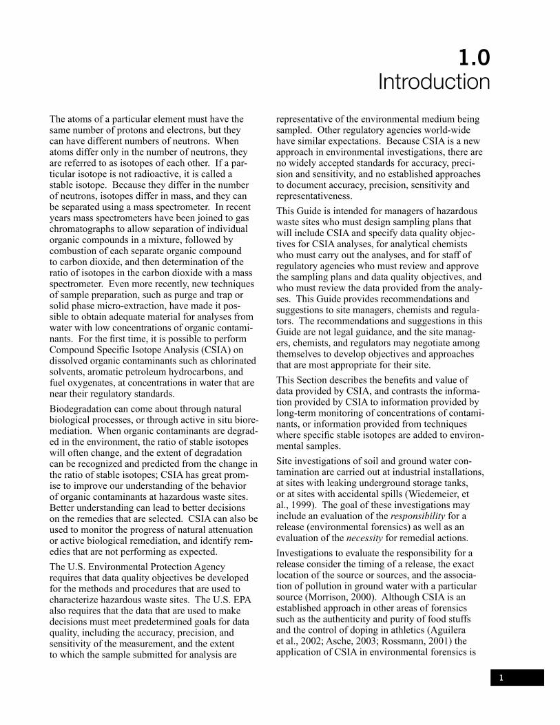
1.0Introduction

The atoms of a particular element must have the same number of protons and electrons, but they can have different numbers of neutrons. When atoms differ only in the number of neutrons, they are referred to as isotopes of each other. If a par-ticular isotope is not radioactive, it is called a stable isotope. Because they differ in the number of neutrons, isotopes differ in mass, and they can be separated using a mass spectrometer. In recent years mass spectrometers have been joined to gas chromatographs to allow separation of individual organic compounds in a mixture, followed by combustion of each separate organic compound to carbon dioxide, and then determination of the ratio of isotopes in the carbon dioxide with a mass spectrometer. Even more recently, new techniques of sample preparation, such as purge and trap or solid phase micro-extraction, have made it pos-sible to obtain adequate material for analyses from water with low concentrations of organic contami-nants. For the first time, it is possible to perform Compound Specific Isotope Analysis (CSIA) on dissolved organic contaminants such as chlorinated solvents, aromatic petroleum hydrocarbons, and fuel oxygenates, at concentrations in water that are near their regulatory standards. Biodegradation can come about through natural biological processes, or through active in situ biore-mediation. When organic contaminants are degrad-ed in the environment, the ratio of stable isotopes will often change, and the extent of degradation can be recognized and predicted from the change in the ratio of stable isotopes; CSIA has great prom-ise to improve our understanding of the behavior of organic contaminants at hazardous waste sites. Better understanding can lead to better decisions on the remedies that are selected. CSIA can also be used to monitor the progress of natural attenuation or active biological remediation, and identify rem-edies that are not performing as expected. The U.S. Environmental Protection Agency requires that data quality objectives be developed for the methods and procedures that are used to characterize hazardous waste sites. The U.S. EPA also requires that the data that are used to make decisions must meet predetermined goals for data quality, including the accuracy, precision, and sensitivity of the measurement, and the extent to which the sample submitted for analysis are

representative of the environmental medium being sampled. Other regulatory agencies world-wide have similar expectations. Because CSIA is a new approach in environmental investigations, there are no widely accepted standards for accuracy, preci-sion and sensitivity, and no established approaches to document accuracy, precision, sensitivity and representativeness.This Guide is intended for managers of hazardous waste sites who must design sampling plans that will include CSIA and specify data quality objec-tives for CSIA analyses, for analytical chemists who must carry out the analyses, and for staff of regulatory agencies who must review and approve the sampling plans and data quality objectives, and who must review the data provided from the analy-ses. This Guide provides recommendations and suggestions to site managers, chemists and regula-tors. The recommendations and suggestions in this Guide are not legal guidance, and the site manag-ers, chemists, and regulators may negotiate among themselves to develop objectives and approaches that are most appropriate for their site. This Section describes the benefits and value of data provided by CSIA, and contrasts the informa-tion provided by CSIA to information provided by long-term monitoring of concentrations of contami-nants, or information provided from techniques where specific stable isotopes are added to environ-mental samples.Site investigations of soil and ground water con-tamination are carried out at industrial installations, at sites with leaking underground storage tanks, or at sites with accidental spills (Wiedemeier, et al., 1999). The goal of these investigations may include an evaluation of the responsibility for a release (environmental forensics) as well as an evaluation of the necessity for remedial actions. Investigations to evaluate the responsibility for a release consider the timing of a release, the exact location of the source or sources, and the associa-tion of pollution in ground water with a particular source (Morrison, 2000). Although CSIA is an established approach in other areas of forensics such as the authenticity and purity of food stuffs and the control of doping in athletics (Aguilera et al., 2002; Asche, 2003; Rossmann, 2001) the application of CSIA in environmental forensics is

2

a recent development (Asche, 2003; Schmidt et al., 2004; Slater, 2003). CSIA has been used success-fully at a variety of sites to distinguish between contaminant releases which occurred at differ-ent times and places at complex spill sites. This knowledge can be used to identify the parties that were responsible for the contamination (Hunkeler et al., 2004; Stark et al., 2003; Walker, et al., 2005) and CSIA has been accepted as one line of evidence in litigation. To determine the need for active remediation, it is useful to have a good knowledge of the behavior of the contaminants in soil and ground water, includ-ing the extent of biodegradation and abiotic trans-formation. This is especially important for passive remedies such as Monitored Natural Attenuation that use naturally occurring processes to attenuate concentrations of contaminants (Wiedemeier et al., 1999).Although natural attenuation has been the focus of many remediation investigations due to its expected economic benefits, it is often difficult to unequivo-cally prove that a contaminant is being transformed in ground water and that the extent of attenuation is sufficient to protect receptors that are down gradi-ent of the source. The standard approach that is usually taken to characterize degradation in the field is to monitor the concentrations of the con-taminant at selected wells and use mass balance calculations to estimate the extent of degradation. This approach has many shortcomings, and the shortcomings are particularly severe for common ground water pollutants that degrade slowly. The conventional approach requires a dense network of monitoring wells, monitoring that extends for long periods of time, and a rather homogeneous aquifer with well-understood hydrogeology. These require-ments are rarely met at real sites, and even when they are, the evidence of degradation is only pro-vided indirectly through a calculation of the miss-ing mass of the contaminant after accounting for all the other processes that might reduce the concentra-tion of the contaminant. These shortcomings have been nicely illustrated in a study of the natural bio-degradation of methyl tertiary butyl ether in ground water at the Borden site in Canada (Schirmer and Barker, 1998). New and different approaches will be required to gain wider acceptance of natural attenuation by regulatory authorities and by the public. If biodeg-radation or abiotic transformation produces a mea-surable change in the ratio of stable isotopes in the contaminant, CSIA may provide direct evidence of the degradation of the contaminant in ground water

at the site (Hunkeler et al., 1999; Meckenstock et al., 1999; Sherwood Lollar et al., 1999). Over the past decade there have been numerous successful applications of CSIA that have demonstrated its potential to recognize and even quantify processes at field scale. CSIA offers a new kind of information that has great economic value to site managers. The tradi-tional approach for monitoring of concentrations of contaminants at sites often does not offer adequate information about the processes that are responsible for removal of the contaminants. Stable isotope analyses can provide an in-depth understanding of biodegradation or abiotic transformation processes in contaminated aquifers. This better understand-ing can improve the conceptual model of the site, which can lead to a more effective remedial strate-gy. The traditional approach of monitoring concen-trations of contaminants can be very costly in the long run. The inclusion of CSIA in the monitoring plan can reduce overall costs by making it possible to reduce the amount of traditional monitoring. Prior to the development of CSIA, isotope techniques relied on changes in the carbon iso-tope ratios of CO2 or DIC (dissolved inorganic carbon) to evaluate the degradation of organic contaminants (Hunkeler et al., 1999). Although this earlier approach can be helpful, it was often difficult to resolve the signal of the carbon that was added to the pool of CO2 or DIC by degradation of the contaminant from the influence of the many other carbon sources and sinks in the subsurface. Furthermore, the sensitivity of the comparison was dependent on the difference in the composition of carbon isotopes in the CO2 produced by biodegra-dation of the contaminants compared to the isotope composition of the background CO2. In addition, the sensitivity of the older technique was often limited by the slow rate of CO2 production from degradation of the contaminant relative to the large pool of DIC in ground water (Dempster et al., 1997 and references therein). In contrast to the earlier techniques, CSIA provides a direct measurement of the isotope ratio in the individual organic contami-nants. Interpretations of CSIA data are much less problematic.There are several new techniques to study biodegra-dation in ground water that involve the addition of contaminants that are artificially labeled with a car-bon isotope (usually 13C-label). Examples include stable isotope probing (SIP) and Bio-Sep® beads amended with 13C-labeled substrates. These tech-niques work in much the same way as radiocarbon labeling; the 13C-label is used to track the transfer

3

of carbon from the substrate to its metabolites, or to the DIC pool, and its subsequent incorporation into the microbial biomass (Geyer et al., 2005; Stelzer et al., 2006). The disappearance of the label from the substrate pool is convincing evidence that the targeted compound is indeed degrading, and the identification of 13C-label in microbial biomass is definitive proof that the compound was biologically degraded. There is an important caveat with these new techniques. Once a substrate with an isotope label has been added to a field site or to micro-cosms, the natural abundance of isotopes has been disturbed to an unpredictable extent, and a funda-mental assumption in the CSIA approach is no lon-ger valid. It is important to choose one approach or the other; they can not be used together.To date, CSIA is most frequently applied to car-bon isotopes, and CSIA for carbon isotopes can be considered to be a mature technique applicable on a routine basis for compounds containing less than ten carbon atoms. With current technology, the heaviest compounds that can be analysed for shifts in the ratio of stable carbon isotopes contain twelve to thirteen carbon atoms. In larger molecules, the isotope shifts are in the range of the experimental error of the isotope analysis (Morasch et al., 2004). Although very promising, isotopic analysis of the other elements currently amenable to CSIA (hydro-gen, oxygen, nitrogen and chlorine), has not been carried out to the same extent as CSIA for carbon isotopes; however, the other elements may become widely used (Berg et al., 2007; Hofstetter et al., 2008; Holmstrand et al., 2006; Sessions, 2006). This guide is focused on biodegradation of organic contaminants in ground water because biodegrada-tion represents the majority of applications to date. Nevertheless, the general principles of CSIA also apply to abiotic transformation reactions. They can be applied to natural materials or to engineered systems such as permeable reactive barriers. This guide can be used for a wide range of applications where reactive processes in ground water produce a change in the ratio of stable isotopes. Currently, CSIA is in transition from a research tool to an applied method that is well integrated into comprehensive plans for management of contami-nates sites. For this reason, the authors felt that it was timely to provide general guidance on good practice for sampling, for measurement, for data evaluation and for interpretation in CSIA based on our experience in research and consulting.

4

Section 2 has primary application for analysts that will analyze samples for CSIA. It explains and defines the delta notation (δ13C and δ2H) that is used to report the stable isotope ratio in a sample. This section explains the nature and source of the refer-ence standards for stable isotope ratios of carbon and hydrogen in organic compounds, provides recommendations on the preparation of laboratory working standards, and the use of working stand-ards to document accuracy, precision, and sensi-tivity of CSIA. It also explains the relationship between the linear range of the continuous flow isotope ratio mass spectrometer and the uncertainty of the determination of δ13C, identifies a threshold in signal strength below which the uncertainty of the determination of δ13C is not stable, and recom-mends that the threshold be used as an operational method detection limit for determination of δ13C. Section 2 provides recommendations for the fre-quency of analysis of CO2 working standards, compound specific working standards, and sample replicates. Finally this section reviews the sensitiv-ity provided by various methods for preparation of the samples for analysis, and the effect of different

methods that can be used to prepare the sample on the value of δ13C that is determined by the isotope ratio mass spectrometer.

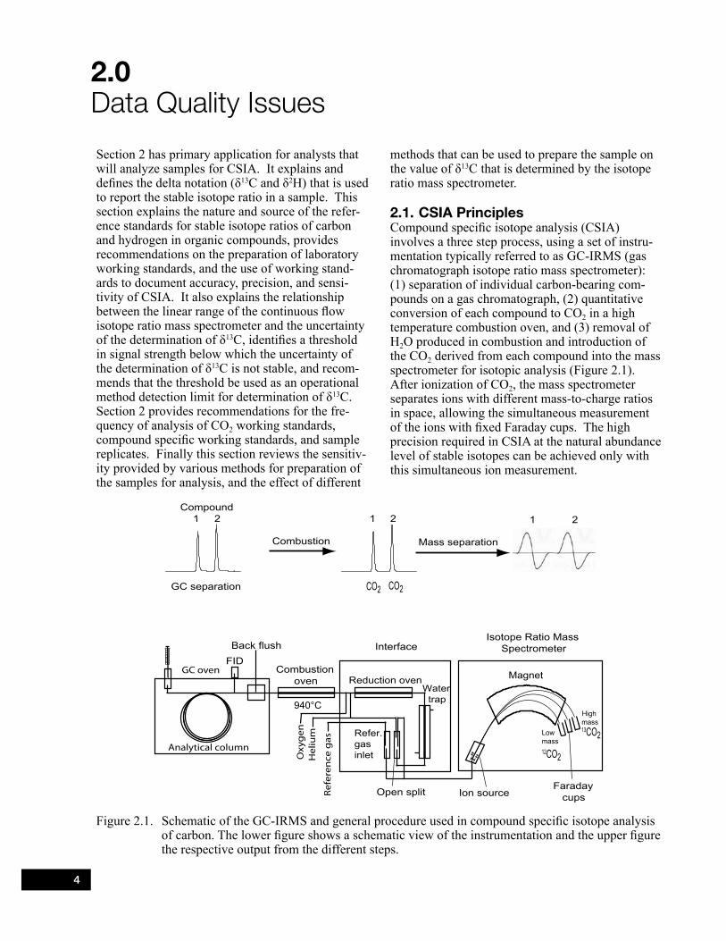
2.1. CSIA PrinciplesCompound specific isotope analysis (CSIA) involves a three step process, using a set of instru-mentation typically referred to as GC-IRMS (gas chromatograph isotope ratio mass spectrometer): (1) separation of individual carbon-bearing com-pounds on a gas chromatograph, (2) quantitative conversion of each compound to CO2 in a high temperature combustion oven, and (3) removal of H2O produced in combustion and introduction of the CO2 derived from each compound into the mass spectrometer for isotopic analysis (Figure 2.1). After ionization of CO2, the mass spectrometer separates ions with different mass-to-charge ratios in space, allowing the simultaneous measurement of the ions with fixed Faraday cups. The high precision required in CSIA at the natural abundance level of stable isotopes can be achieved only with this simultaneous ion measurement.

2.0 Data Quality Issues

Analytical column

Combustion oven

Open split

GC oven

Faraday cups

Reduction oven Magnet

High mass

Low mass

Ion source

Isotope Ratio Mass Spectrometer

940°C

Water trap

InterfaceFIDBack flush

13CO212CO2

Combustion

GC separation

1 2 1 2 1 2

CO2 CO2

Mass separation

Ox

yge

nH

eliu

m

Re

fere

nce

ga

s

Compound

Refer. gas inlet

Figure 2.1. Schematic of the GC-IRMS and general procedure used in compound specific isotope analysis of carbon. The lower figure shows a schematic view of the instrumentation and the upper figure the respective output from the different steps.

5

2.2. Nomenclature and International Standards

Stable isotope analysis of carbon or hydrogen involves measurement of the relative abundance of the two stable isotopes of carbon (13C and 12C) or hydrogen (2H and 1H). In order to ensure inter-laboratory comparability and accuracy, these ratios are expressed relative to an international standard (typically V-PDB for carbon and V-SMOW for hydrogen). Measured values are reported as δ13C and δ 2H respectively. These terms are defined in Equations 2.1 and 2.2 as follows:

( ) ( ) ( )( )

13 12 13 12sample standard13

13 12

standard

C C C CC 1000

C C

− δ = ×

000

2.1

( ) ( ) ( )

( )2 1 2 1

sample standard22 1

standard

H H H HH 1000

H H

− δ = ×

000 2.2

Since the resulting δ values are very small (for δ13C typically < 0.05), they are generally multiplied for convenience by 1000 and reported as parts per thousand or “per mill”, indicated by the symbol ‰. Sometimes, the standard is explicitly indicated after the ‰ symbol, e.g. for carbon isotopes the values are reported as ‰ V-PDB. If no information is given, it can be assumed that the values are report-ed relative to the usual standard material.For decades the International Atomic Energy Agency (IAEA) in Vienna, in conjunction with the National Bureau of Standards in the United States, has administered and overseen the storage and distribution of the key international stable isotope standards. Analysis and reporting of the other stable isotope systems (O, N, Cl, etc.) follow an analo-gous approach (Clark and Fritz, 1997). In the common delta notion, the deviation of the stable isotope value of the sample from the standard will be either negative or positive. A negative value means that the sample is depleted in its 13C-content relative to the 13C/12C content of the standard whereas a positive sign implies an enriched 13C-content. According to the IUPAC definition, compounds that only differ in their isotope composition (such as 12CO2 and 13CO2) are called isotopologues. The term “isotopomer” is used for isomers having the same number of each isotopic atom but differing in their positions. As an example, Cl2

12C-13CHCl and

Cl213C-12CHCl are the two isotopomers of TCE with

respect to carbon.In the following sections we will focus on data quality issues of carbon isotope analysis since car-bon is by far the most frequently measured element in CSIA to date.

2.3. Laboratory Working StandardsThe following sections are intended primarily for laboratory staff that will actually analyze the samples, and for staff that will prepare or review Quality Assurance Project Plans.

2.3.1. CO2 Reference GasSince the international standard materials are made available to each laboratory in limited amounts, they are not used for daily operations and measure-ments. For daily operations and standardization, each laboratory obtains pure CO2 reference gas and cross-calibrates it against the international standard materials to develop in-house working standards. To obtain maximum accuracy, this cross-calibration should be done by the conventional dual inlet approach; alternatively, the isotope composition of working standards can be determined by an elemental analyser - isotope ratio mass spectrom-eter (EA-IRMS). Once the laboratory’s working CO2 standard is characterized (1) it should be used daily to calibrate the isotope ratio mass spectrom-eter, (2) the CO2 working standard should be cross-checked against the international standard materials every few months to ensure continued accuracy, and (3) aliquots of the CO2 working standard should be stored in glass ampoules so it can be available on a long term basis for calibration checks and quality control, and for inter-laboratory com-parisons. See Coplen et al., (2006) and Qi et al., (2003).

2.3.2. Compound specific Working Standards

The CO2 working standard is included in individual sample sets to act as an internal standard. Since organic compounds may behave differently in this analytical system than pure CO2 (due to differ-ences in chromatographic separation, combustion efficiency, peak shape, etc.), it is important for each laboratory to also characterize compound specific working standards for the target compounds that they typically analyze (Figure 2.2). Isotopic characterization of the working standards should be done off-line using the sealed quartz tube combustion technique and conventional dual inlet mass spectrometry to ensure maximum preci-sion and accuracy with respect to the international

6

standard (V-PDB) and the laboratory CO2 work-ing standard. Typical precision for this approach is ± 0.15‰ (Clark and Fritz, 1997). There is an increasing trend to measure the isotopic composi-tion of organic working standards by an elemen-tal analyser - isotope ratio mass spectrometer (EA-IRMS) which is appropriate as long as the careful procedures outlined in Qi et al. (2003) are followed.The following recommendations for archiving and storage of compound specific working standards are for compounds that are liquid at room tempera-ture and pressure. Purchase pure product for each compound to be analyzed. Ensure highest purity as even small amounts of contaminants can affect the ability to accurately characterize the compound of interest. At least two dozen sealed glass ampoules should be set aside as ARCHIVED standards for use when needed to cross-check the isotopic value in the future, or for inter-laboratory comparisons. Set up a second set of thirty to forty sealed glass ampoules to be used as WORKING standards for

daily standardization, controls on experiments, and for correcting problems with the performance of the instrument. It is advisable to test the procedure used to seal the ampoule to insure that the ampoules are flame-sealed quickly. If significant amounts of compound are lost through volatilization, this might change the isotopic ratio of the standard.

2.4. Method Testing, Quality Assurance and Quality Control

Conventional off-line preparation techniques and dual inlet isotope ratio mass spectrometry (IRMS) provide optimized analytical conditions to obtain maximum precision. In contrast, continuous flow IRMS provides for rapid analysis of complex mixtures of organic compounds, and for dissolved organic compounds in environmental samples. Continuous flow IRMS requires a sample size that is approximately four to five orders of magnitude smaller than the sample needed for off-line prepara-tion techniques. Continuous flow IRMS however produces an inevitable loss of precision. The loss

Figure 2.2. Example of a chromatogram obtained in GC-IRMS. Upper panel: Isotope ratio trace with the typical isotope swings due to the partial separation of isotopologues prior to on-line combus-tion caused by the inverse isotope effect in gas chromatography (modified after Jochmann et al. 2006). Lower panel: Gas chromatograph. Note that the CO2 working standard produces the flat-top peaks at the start of the chromatogram.

7

of precision is related to a wide variety of factors which are beyond the scope of this Guide but which include a higher source pressure for the helium car-rier gas, higher background concentrations of water, and the need to tune the source for optimum linear-ity rather than optimum sensitivity. In the follow-ing sections, we provide an approach to determine reasonable values for reproducibility, accuracy and the detection limit for compound specific work-ing standards that are analyzed by continuous flow mass spectrometry, and provide attainable goals for reproducibility, accuracy and detection limits for CSIA data (for more detail see Sherwood Lollar et al., 2007; Jochmann et al., 2006).

2.4.1. Reproducibility Reproducibility (or precision) refers to the ability to obtain the same value when the same sample or standard is analyzed repeatedly (Figure 2.3). In compound specific isotope analysis (CSIA), if a sample is run in duplicate or triplicate under con-stant operating conditions, the standard deviation of the mean of the replicate measurements is typically <0.1 to 0.3‰ for δ13C values. While reproducibility is necessary to minimize uncertainty, it is not a suf-ficient expression of the total degree of uncertainty (error) in a measurement. As illustrated in Panel C of Figure 2.3, a measurement can be highly repro-ducible (precise) but nevertheless be inaccurate.

Figure 2.3. An illustration the difference between precision (reproducibility) and accu-racy of several data points, using the bull’s eye of a target as the goal for high accuracy and good precision.

2.4.2. Total Uncertainty and the Critical Role of Linearity

When a suite of real samples are analyzed by CSIA, all the operating conditions are not held constant from one run to the next as described above in the definition of analytical precision. In fact, one of the key advantages of continuous flow CSIA is that it permits, in the same analytical run, the measure-ment of the δ13C values for several compounds that are present in the sample mixture at different con-centrations. However, specific sample preparation parameters, such as split ratios, are often adjusted to bring the concentration of all of the analytes into the linear range of the instrument. In contrast to conventional dual inlet systems where the stand-ard peak size must be carefully balanced to match the sample peak size, in continuous flow CSIA the standards can be input at one peak size (typically 1 to 2 Volts) and then used to characterize sample peaks that are either above or below that size. The linear range, the range over which accurate meas-urements are possible, varies from instrument to instrument. The linear range depends on the mass spectrometer itself as well as the chromatograph and combustion system. As used in analytical chemistry, the term linear-ity usually refers to a linear increase of the signal with increasing amount of analyte. As applied to isotope analysis, linearity indicates that (within an acceptable range) the obtained isotope ratio is independent of the amount of compound injected. The following sections provide further details on how to establish the linearity of the CSIA analytical system and the implications that linearity has for documenting the uncertainty and detection limits associated with isotope ratios (see also Sherwood Lollar, et al., 2007).Figure 2.4 shows the results of a typical linearity test. Multiple analyses of a laboratory working standard for TCE were run under identical opera-tional parameters including constant concentration of TCE, and constant chromatographic conditions, combustion temperature, flow rate, and split setting. However, a wide range of different peak sizes (or signal sizes) were obtained by varying the amount of sample introduced. When this type of test is car-ried out, for any given measurement, the δ13C value obtained is typically within ± 0.5‰ of the value for the laboratory working standard obtained by off-line preparation techniques and dual inlet mass spectrometry. Based on these results a sample that is run under similar conditions should also have a total uncertainty of approximately ± 0.5‰. As illustrated in Figure 2.4, there is a threshold in the size of the signal below which the variation for

8

replicate values of the working standard increases significantly. The values of δ13C that are measured below this threshold can be more enriched than the standard value, or less enriched than the standard value, and whether they are more or less than the standard value varies with time under constant operating conditions - hence no corrections should be attempted for values of δ13C that are measured below the threshold. See also Jochmann, et al. (2006) and Sherwood Lollar, et al. (2007).

Figure 2.4. Typical linearity test of a laboratory working standard run by CSIA over a wide range of different peak sizes (or signal sizes) by varying the amount of analyte introduced. Modified after Sherwood Lollar et al. (2007). The solid line is the mean of all the repli-cate analyses of the working standard. The dotted lines are ± one standard deviation of the mean.

The largest effects on the value of δ13C are typi-cally attributable to the effects of sample size on linearity or to a change in a major parameter such as purposely changing the split setting. The effects of these changes vary somewhat from compound to compound. Therefore it is highly recommended to document the effect of changes in these para-meters on the measured value of δ 13C for each compound specific working standard. The total uncertainty varies from compound to compound. Maintenance of a control chart to monitor this variation is an important part of good practice for Quality Assurance/Quality Control (QA/QC). In any laboratory inter-comparison, values measured from one laboratory to another should agree within ± 0.5‰ (or other level of uncertainty specific to a particular compound) if each laboratory has prop-erly calibrated their working standard to V-PDB.

Sherwood Lollar et al. (2007) and references there-in demonstrate that a total uncertainty of ± 0.5‰ is typical for many hydrocarbon contaminants investi-gated to date, including alkanes, certain chlorinated ethenes, certain chlorinated ethanes and aromatic hydrocarbons. However, at the current state of practice for CSIA, an uncertainty of ± 0.5‰ can not be routinely attained for analysis of carbon isotopes in every volatile organic compound that might be of regulatory interest. It is the responsibility of the analyst to provide documentation of the upper limit on uncertainty that is associated with a particular compound of interest when analyzed following a particular protocol for CSIA. It is the responsibil-ity of the user of the data to determine whether the achieved upper limit on uncertainty is acceptable for their particular application.

2.4.3. Establishing Concentration Thresholds or “Detection limits”

Mass spectrometry can produce a δ 13C value for very small signals. However, as indicated above, at signal sizes below a certain threshold both the accuracy and reproducibility of δ 13C measurements deteriorate. We recommend that the operational detection limit be defined as that concentration of the compound in the water sample below which the accuracy and reproducibility of the value for δ 13C deteriorate beyond acceptable limits. The crite-rion for “acceptable limits” depends on the use of the data, and is dependent on the methods and the instruments used. As mentioned above, for many compounds of interest, most laboratories can attain a standard deviation of the mean of triplicate sam-ples of ±0.5‰ for CSIA of carbon. Jochmann et al. (2006) compared the variation in δ 13C in triplicate analyses over a range of concentrations. They com-pared the data to identify the concentrations that met two criteria: the mean value of triplicate mea-surements at a particular concentration was within ±0.5‰ of the mean of all analyses over the range of concentrations, and the standard deviation of the triplicate analyses at a particular concentration was less than ± 0.5‰, as is illustrated in Figure 2.5. They defined the method detection limit as the low-est concentration that satisfied both of the criteria.The minimum quantity of sample necessary to keep the uncertainty in the determination of the isotopic ratio within acceptable limits will vary from com-pound to compound and may also depend on the technique used to prepare the samples for analysis. For any particular technique to prepare the sample, the minimum quantity will be associated with a minimum concentration necessary to keep uncer-tainty within acceptable limits. This minimum

9

concentration becomes the effective detection limit for determination of isotopic ratios. It therefore should be established separately for each compound and each injection/preconcentration technique using compound specific working standards. In the example shown in Figure 2.5, the MDL for benzene is 0.2 µg/L, which corresponds to a peak height of 250 mV. As discussed above, it is not generally possible to “correct” for values run at smaller signal sizes. Ideally, improving detection limits for CSIA relies on increasing the efficiency of sample preparation and preconcentration steps to provide higher sig-nal peaks (see below), and not by trying to “cor-rect” values or simply to report values close to the threshold at which the accuracy of the determina-tion will be compromised.

2.4.4. Application of These Principles to Other CSIA Measurements

For hydrogen isotopes, the principles for establish-ing reproducibility, total uncertainty and detection limit are the same as for carbon isotopes. However, there are few formal studies on the uncertainty associated with analysis of δ2H in environmen-tal investigations, and we will not make specific performance recommendations at this time. As a

rule of thumb the total uncertainty for hydrogen is usually at least an order of magnitude greater than for carbon; total uncertainty for δ 2H is typically ± 5‰ versus ± 0.5‰ for δ 13C (Sherwood Lollar et al., 2007). For an example of this kind of method development for hydrogen isotope analysis see Gray et al. (2002). Similar principles will be appli-cable to H, N, Cl, S, and O using continuous-flow compound specific methods. See Sessions (2006) for an extensive review of analytical methods. As with any new method, there may be other important operational parameters in addition to those that affect carbon and hydrogen CSIA measurements and careful work is needed.

2.4.5. Extraction Methods for CSIA Based on the requirements specified by the vari-ous manufacturers of isotope ratio mass spectrom-eters, it is necessary to inject approximately 1 nmol carbon or 8 nmol hydrogen on column to have adequate mass to provide an accurate and precise measurement of the isotope ratio. These criteria assume that the GC-IRMS instrument is tuned to maximum linearity, and that the chromatographic resolution (Rs) is greater than 1.5, which provides narrow peaks with good peak separation.

Figure 2.5. Example of the evaluation of method detection limits (MDLs) in CSIA. The squares represent the δ13C values in ‰ and the diamonds show the amplitude of mass 44 in mV. Error bars indicate the standard deviation of triplicate measurements. The horizontal broken line represents the iteratively calculated mean value after the methods of Jochmann et al. (2006) and Sherwood Lollar et al. (2007). The solid lines around the mean value represent the standard deviation on the mean of triplicate measurements. Figure modified after Jochmann et al. (2006).

10

These criteria can be used to estimate the mass of individual compounds that must be delivered on column:

1 for carbon

xi inmolm M= 2.3

and

8 for hydrogenxi i

nmolm M= 2.4

where mi is the required mass in ng, x is the num-ber of carbon or hydrogen atoms respectively in the compound, and Mi is the molecular weight of the compound in g/mole.For methyl tertiary butyl ether, for example, this yields a minimum mass of 18 ng. Using a dimen-sionless air-water partition constant Kaw of 0.12 at 50 °C (Arp and Schmidt, 2004) for a typical head-space extraction (10 mL sample and 10 mL head-space, 1 mL gas injection, 50 °C) this is equivalent to a concentration in the water sample of 170 µg/L. For hydrogen, at least 8 nmol are required and the same calculation as above yields 59 ng or 550 µg/L. These are calculated minimum numbers under optimum conditions and, as Table 2.1 shows, are often not achievable. Unfortunately, environmen-tal concentrations of interest are frequently below these levels, especially at contaminated sites out-side the plume core or if substantial degradation has occurred. Efficient extraction or preconcentration techniques must be integrated with GC-IRMS in order to fully exploit the potential of the method for a wide range of samples, in particular for ele-ments other than carbon. To meet this need, over the past few years several studies have worked to lower the detection limits for CSIA by the use of sorptive extraction techniques such as solid-phase microextraction (SPME) or purge and trap (P&T). Note that almost all these studies have focused on compounds that are relatively water soluble and volatile, such as the BTEX compounds, MTBE, and chlorinated ethylenes. These compounds are among the most common industrial ground water pollutants. The concentration thresholds or effective detection limits are constrained by the physical limits of the gas chromatograph isotope ratio mass spectrometer system, as well as by the technique used to prepare the sample. Ideally, the extraction or preconcenta-tion technique will be free of isotope fractionation effects and will be adequate to concentrate enough material from each compound of interest to deter-mine the isotopic ratio at concentrations that are relevant to plumes of contaminated ground water.

Table 2.1 summarizes the effective detection limit that has been reported for a variety of techniques that are used for sample preparation prior to CSIA of the common organic contaminants in ground water. As a first approximation, the sensitivity is correlated with the molar concentration of carbon (or any other element of interest) of the compound in the sample. Limits of detection should be deter-mined based on the lower range of linearity of the instrument (see Section 2.4.3). However, Table 2.1 provides the concentration corresponding to the typical operational limits of detection, based on the criteria of 1 nmol carbon and 8 nmol hydrogen on column and our experience with the technique. Detection limits for nitrogen or oxygen isotope analysis are provided by the manufacturer of the instrument. However, there are only a few methods available for extraction and preparation of samples, or protocols available for CSIA, that are appli-cable to isotopes of nitrogen, chlorine, and oxygen in ground water contaminants (Berg et al., 2007; Hartenbach et al., 2006; Holmstrand et al., 2006; Penning and Conrad, 2007). Studies for hydrogen isotope analysis of ground water contaminants are also still relatively limited (Kuder et al., 2005; Mancini et al., 2002; also Table 2.1).A prerequisite for the selection of any extraction or preconcentration technique used to prepare samples for CSIA is adequate sensitivity. A further prerequisite is a negligible change in the value of δ13C or δ2H during the extraction or enrichment process, or at least a highly reproducible change. Before an extraction or preconcentration technique is implemented on a routine basis, it is mandatory to thoroughly evaluate the technique for changes in the value of δ13C or δ2H during sample prepara-tion, rather than relying on data reported by oth-ers. The change in the value of δ13C or δ2H may vary depending on analytical conditions such as the split ratio and extraction time. Each compound that will be analyzed should be tested using work-ing standards with a known isotopic composition (see Section 2.3). The evaluation should cover the typical range of operating conditions. The standard deviation of replicate analyses should typically be smaller than ±0.5‰ for carbon, otherwise the method is not suited for typical applications. A number of extraction methods have been shown to provide accurate isotope ratios, while other methods change the value of δ13C or δ2H (Table 2.1). There are some general trends. Typically headspace and direct immersion SPME are not accompanied by a substantial changes in the value of δ13C or δ2H (Dayan et al., 1999; Slater et

11

al., 1999; Dias and Freeman, 1997; Hunkeler and Aravena, 2000b; Zwank et al., 2003). If changes in the value of δ13C or δ2H are observed with SPME, the analyte tends to be depleted in 13C compared to pure phase standards, i.e., the lighter compound partitions more strongly into the fiber which is then subsequently analyzed. This resembles the same inverse isotope effect that is observed in gas chromatography. Although this effect is often quite small, for carbon tetrachloride, Zwank et al. (2003) found high deviation using direct immersion SPME, which could not be explained. Furthermore, Hunkeler et al. (2001a) found a significant 13C-depletion of tertiary butyl alco-hol extracted by SPME. Sometimes significant inverse isotope effects are seen during headspace equilibration with an aqueous sample. An enrich-ment of 13C in the gas phase of up to 1.46‰, has been observed (Hunkeler and Aravena, 2000b), thus Hunkeler et al. (2005) applied corrections in sub-

sequent work in order to allow for a comparison of isotope data generated with different methods. There is no consistent pattern in the changes in the value of δ13C or δ2H. Compounds other than ter-tiary butyl alcohol behave differently (Slater et al., 1999), which emphasizes the need for testing each individual compound during method validation. Dynamic extraction methods such as purge and trap and dynamic headspace extraction aim for a quanti-tative (100%) extraction of the sample with subse-quent trapping and thermo-desorption of the analyte into the GC column. These dynamic extraction methods are more appropriate for isotope analysis at very low concentrations. In the various studies conducted to date that used an adequate purge time, no significant change in the value of δ13C or δ2H has been reported. Zwank et al. (2003) have shown for a number of volatile organic compounds that sample preparation does not compromise the analy-sis unless the extraction efficiencies drop below approximately 40%.

Table 2.1. Extraction or sample preparation techniques used in CSIA for volatile ground water pollutants. Adapted and updated from Schmidt et al. (2004).

CompoundInjection/

preparation technique

Change in the value of δ13C or δ2H during

analysis

Definition of the Detection Limit

Operational Detection limit

[µg/L]Reference

δ13C δ2HMethyl Tertiary

Butyl Etherliquid

injectionaOCb <0.3‰;

SLc ~1‰ Amplitude > 0.5 V 24000 - (Zwank et al., 2003)

headspace injection n.s.c.e Amplitude > 0.5 V 5000 50000 (Gray et al.,

2002)

Amplitude > 0.5 V4000

(TAME: 6000)

- (Somsamak et al., 2005)

headspace SPME

C: -0.9‰ H: -17‰

(both with resp. to HS injection)

Amplitude > 0.5 V 350 1000 (Gray et al., 2002)

headspace SPME

Significant but small change

(-0.67±0.21‰)Amplitude > 0.75 V 11 - (Hunkeler et

al., 2001a)

direct immersion

SPME

Reproducible change

(<0.5‰), but presence

of BTEX concentrations

>3 mg/L caused 2‰ deviation.

Amplitude > 0.5 V 16 - (Zwank et al., 2003)

12

CompoundInjection/

preparation technique

Change in the value of δ13C or δ2H during

analysis

Definition of the Detection Limit

Operational Detection limit

[µg/L]Reference

δ13C δ2H

P&TSmall shift of δ13C values (+0.33‰)

n.r.d 15 - (Smallwood et al., 2001)

P&T n.r.d n.r.d 5 - (Kolhatkar et al., 2002)

P&T n.s.c.e Amplitude > 0.5 V 0.63 - (Zwank et al., 2003)

P&T n.r.d < 0.5‰ precision 2.5 20 (Kuder et al., 2005)

Benzene liquid injectiona n.s.c.e Amplitude > 0.5 V 19000 - (Zwank et

al., 2003)headspace injection n.s.c.e Amplitude > 0.5 V 500 - (Mancini et

al., 2003)direct

immersion SPME

n.s.c.e Amplitude > 0.5 V 22 - (Zwank et al., 2003)

P&T n.s.c.e Amplitude > 0.5 V 0.30 - (Zwank et al., 2003)

P&T n.r.d

Moving mean within ± 0.5‰

interval and s < 0.5‰

0.20 - (Jochmann et al., 2006)

Toluene liquid injectiona

OCb n.s.c.e SLc~-1‰ Amplitude > 0.5 V 9500 - (Zwank et

al., 2003)

headspace injection n.s.c.e Amplitude > 2 V - 2000 (Ward et

al., 2000)headspace injection n.s.c.e Amplitude > 0.2 V 100 - (Slater et

al., 1999)

direct immersion

SPME n.s.c.e

Peak area equiv. to 50 pmol CO2 at the

ion source (ca. 0.7 Vs)

45 -(Dias and Freeman,

1997)

direct immersion

SPME n.s.c.e Amplitude > 0.5 V 9 - (Zwank et

al., 2003)

P&T n.s.c.e Amplitude > 0.5 V 0.25 - (Zwank et al., 2003)

P&T n.s.c.eMoving mean with-in ± 0.5‰ interval

and s < 0.5‰0.07 - (Jochmann

et al., 2006)

Chlorinated Methanes

liquid injectiona

CHCl3, ~-1.5‰CCl4, OCb

-3.31±0.34‰Amplitude > 0.5 V

170000 to

220000- (Zwank et

al., 2003)

13

CompoundInjection/

preparation technique

Change in the value of δ13C or δ2H during

analysis

Definition of the Detection Limit

Operational Detection limit

[µg/L]Reference

δ13C δ2H

direct immersion

SPME

CHCl3, -1.8±0.28‰

CCl4, -7.3±0.22‰

Amplitude > 0.5 V170 to

280- (Zwank et

al., 2003)

direct immersion

SPME

n.s.c.e -0.09 to 0.40 ‰

1.5 nmol C on column

360 to 2200 -

(Hunkeler and

Aravena, 2000b)

headspace injection 1.03 to 1.29 ‰ 1.5 nmol C on

column800 to 3300 -

(Hunkeler and

Aravena, 2000b)

P&T CHCl3 and CCl4, n.s.c.e Amplitude > 0.5 V ≤5.0 - (Zwank et

al., 2003)

P&TCHCl3, ~-1.5‰CCl4 and DCM,

n.s.c.e

Moving mean within ± 0.5‰

interval and s < 0.5‰

18 to 27 - (Jochmann et al., 2006)

Chlorinated Ethenes

liquid injectiona

Small but significant

change observed for TCE and

cis-DCE

Amplitude > 0.5 V71000 to

84000- (Zwank et

al., 2003)

headspace injection TCE, n.s.c.e Amplitude > 0.2 V 400 - (Slater et

al., 1999)

direct immersion

SPME n.s.c.e

-0.37 to +0.06‰1.5 nmol C on

column130 to

290 -(Hunkeler

and Aravena, 2000b)

headspace injection 0.21 to 0.69 ‰ 1.5 nmol C on

column170 to 1000 -

(Hunkeler and

Aravena, 2000b)

direct immersion

SPME

Small (~1‰) but significant

change observed for cis-DCE

only

Amplitude > 0.5 V66 to130

- (Zwank et al., 2003)

P&T n.s.c.e Not given 5 - (Song et al., 2002)

P&T

Small (~0.7‰) but significant

change observed for cis-DCE

only

Amplitude > 0.5 V 1.1 to 3.6 - (Zwank et

al., 2003)

14

CompoundInjection/

preparation technique

Change in the value of δ13C or δ2H during

analysis

Definition of the Detection Limit

Operational Detection limit

[µg/L]Reference

δ13C δ2H

P&T n.s.c.e

Moving mean within ± 0.5‰

interval and s < 0.5‰

0.8 to 5.1 - (Jochmann

et al., 2006)

dynamic headspace extraction

n.s.c.e Amplitude > 0.2 V 10 to 38 - (Morrill et al., 2004)

Misc. Compounds

Methyl-cyclohexane

direct immersion

SPME< 0.5 ‰

Peak area equiv. to 50 pmol CO2 at the ion source

(ca. 0.7 Vs)24 -

(Dias and Freeman,

1997)

Alkylated Benzenes P&T n.s.c.e

Moving mean with-in ± 0.5‰ interval

and s < 0.5‰0.07 to

0.35 - (Jochmann et al., 2006)

Hexanoldirect

immersion SPME

< 0.5 ‰Peak area equiv. to 50 pmol CO2 at the ion source

(ca. 0.7 Vs)4200 -

(Dias and Freeman,

1997)

Tertiary Butyl

Alcohol

direct immersion

SPME

Significant change

(-1.18±0.12‰)Amplitude > 0.75 V 360 -

(Hunkeler et al.,

2001a)TertiaryButyl

AlcoholP&T n.r.d < 0.5‰ precision 25 - (Kuder et

al., 2005)

Bromoform, Ethylene

DibromideP&T n.r.d

Moving mean with-in ± 0.5‰ interval

and s < 0.5‰14, 3.9 - (Jochmann

et al., 2006)

Nitro- aromatic

compounds

direct immersion

SPME

Significant change for some compounds (up

to -1.3‰)

Amplitude > 0.5 V (equiv. to ca.

0.8 nmol C on column)

73 to 780 - (Berg et al.,

2007)

Anilinesdirect

immersion SPME

Significant change for some compounds (up

to 1.1‰)

Amplitude > 0.5 V (equiv. to ca.

0.8 nmol C on column)

320 to 1600 - (Berg et al.,

2007)

a Analyte dissolved in solvent. b On column injection. c Splitless injection. d Not reported in reference. e No significant change (<0.5‰) observed.

15

2.5. Avoiding Some Pitfalls in CSIA Measurements

Sessions (2006) gives an excellent overview of requirements for successful isotope analysis. Blessing et al. (2008) recently discussed potential pitfalls in CSIA of environmental samples. Some of their recommendations are summarized here.Many analysts nowadays are accustomed to the selectivity provided by mass spectrometric detec-tors in quantitative analysis. However, the continu-ous flow GC-IRMS is non-selective. In the case of carbon, all of the compounds are converted to CO2 before analysis of the isotopic ratio. The system “sees” all the carbon (or other element) eluted from the column. Therefore, it is of the utmost impor-tance to remove coeluting non-target compounds as completely as possible or to modify separation methods to allow a baseline separation. Samples should be screened by GC/MS or GC/FID prior to CSIA measurements to avoid overloading of the GC-IRMS system with non-target analytes. If the interfering compounds are sufficiently sepa-rated from the target analytes, they can be elimi-nated by switching a valve installed between the GC column and the combustion oven. The valve diverts the flow of carrier gas with the interfering compounds away from the combustion oven.Peak integration should be closely monitored and adjusted manually if necessary. This is a much more delicate task than in quantitative analysis because shifting the peak delimiters can significantly change the calculated isotope values due to the partial chromatographic separation of isotopologues. Isotope swings can serve as good indicators of peak quality. A correction can be applied with care to account for material that bleeds from the GC column. Use of CO2 standards within the sample run is helpful to provide the “ground-truth” for such corrections. Data can be automatically corrected using various algorithms that are available for this purpose in commercial instruments. However, at the time of this writing (Spring 2008) a thorough comparison of the various methods has not been conducted (Sessions, 2006).

2.6. Recommended Routine for Daily Laboratory Quality Assurance/Quality Control (QA/QC) for Carbon Isotope Analysis

Test the linearity and sensitivity of the instrument with the CO2 working standard. Then test the lin-earity of the instrument with the compound specific working standards over a typical range of operating conditions that will be used for the day’s samples. Operating conditions include the range of concen-trations, split or flow settings, and the technique used to prepare the samples, such as a headspace sampler, SPME or purge and trap. Values of δ13C for each standard typically should remain within ± 0.5‰ (1 σ) of the previously determined isotopic working standard value to ensure both accuracy and reproducibility. Plotting these values on a con-trol chart will allow for continuous monitoring of QA/QC over the long term.Analyze samples under the same conditions as above, ensuring baseline separation for the target compounds. Requirements for excellent chromatog-raphy are even more stringent than for concentra-tion analysis.At a minimum, the CO2 working standard should be analyzed at the beginning of each sample run. At least every fifth sample should be a replicate. At least every tenth sample should be the compound specific working standard.All samples should stay within the previously established range of acceptable linearity and above the established threshold limit. If a sample falls outside the acceptable range, the concentrations of the analytes should be adjusted, if possible, to bring the sample within the established range, and the sample analyzed a second time. Follow the specifi-cations provided by the manufacturer of the instru-ment for the upper limit of the range of linearity.

16

This section provides specific recommendations for collection, preservation and storage of ground water samples that are intended for CSIA analysis. The section has application to the development of Quality Assurance Project Plans for site characterization, and is intended for contractors that sample ground water, and for site managers and regulators that develop and approve sampling plans.

3.1. Collection of Ground Water from Monitoring Wells

Procedures and conditions that would compromise a sample intended for analysis of concentrations of a particular organic contaminant will also com-promise the sample for CSIA analysis. Procedures and conditions that sustain and maintain the suit-ability of a sample for analysis of concentrations of a particular organic contaminant will also sustain and maintain the suitability of the sample for CSIA analysis. As a general rule, established good prac-tice for acquisition of samples for analysis of con-centrations of organic contaminants can be accepted as good practice for samples intended for CSIA analysis. In particular, criteria for methods of pres-ervation, for methods for shipping samples from the field site to the laboratory, and criteria for holding times and holding temperatures to store samples that have been established for analysis of concen-trations of organic contaminants are also applicable to CSIA analyses. U.S. EPA has provided recommendations and guidance on collecting ground water samples (Barcelona et al., 1985; Yeskis and Zavala, 2002) and a comprehensive description of good practice for ground water sampling is available in Nielsen (2006).Ground water can be collected from monitoring wells by a variety of devices including bailers, above ground peristaltic pumps with plastic sam-pling tubes inserted into the well, and down-hole pumps (Nielsen, 2006). Any of the devices can produce an adequate sample if they are used appro-priately. To minimize the loss of volatile analytes, the device should be used in a manner that mini-mizes the exposure of the ground water sample to the atmosphere during sampling.

If a well is not purged before sampling, the water pumped from the well may or may not be repre-sentative of the ground water in the aquifer being sampled (Nielsen, 2006). Volatile compounds can be lost to the headspace above the water column in the well. Oxygen from the air above the water in the well can diffuse into the water and support aerobic biodegradation of organic compounds in the water in the well that might not occur in the ground water in anoxic aquifers. There are two general approaches to purge the water from the well before it is sampled for chemi-cal analysis. In the first approach, the volume of water contained in the casing of the well is calcu-lated from the depth of the water column in the well and the diameter of the well, then two or three casing volumes of water are purged from the well before the well water is sampled. In the second approach, field instruments are used to continuously monitor sensitive parameters such as temperature, redox potential, and concentrations of dissolved oxygen in the water purged from the well. The samples are taken after the sensitive parameters become stable (Yeskis and Zavala, 2002). Depending on the vertical interval screened by a monitoring well, on the vertical distribution of hydraulic conductivity, and on the vertical extent of concentrations of contaminants in ground water, the concentrations of contaminants in well water may change over time as a well is purged. Figure 3.1 presents a common scenario where this situation might be expected. Ground water contamination is present in an aquifer in the flood plain of a major river. The land surface is comprised of silts and clays of the flood plain, while sands and gravels from old meanders of the river occur at depth. The water table occurs in the silts and clays, and the monitoring well is screened in the silts and clays. Contaminated ground water moves through the layers of sand and gravel because they have higher hydraulic conductivity.When the monitoring well is pumped to a mod-est extent, it will produce water from the silts and clays. This water often is recent recharge water from precipitation, and is free of contamination. When the well is purged more extensively, con-taminated water is drawn in from the deeper, more

3.0Collection, Preservation and Storage of Samples

17

hydraulically conductive intervals. The actual physical relationship between water bearing units that are sampled after modest purging and the units sampled after extensive purging will vary from one site to another. However, all aquifers are to some extent heterogeneous, and similar effects can be expected at most sites. The concentrations of contaminants can go up or down as a well is purged more extensively. Aquifer heterogeneity is dis-cussed in more detail in Section 4.5.To select appropriate wells for concentration and isotope analysis, it is necessary to know the rela-tionship between the screen of the monitoring well and the various units in the aquifer that can yield ground water to the monitoring well. If a well has a short screen that is installed near the center of a transmissive sand and gravel unit, the geochemi-cal parameters will likely stabilize when the well is purged, and the concentrations of contaminants in the well water will be representative of the aquifer unit that is being sampled. If a well has a long screen that extends between layers of sand or gravel and layers of silt or clay, the well will sample different aquifer units that may have differ-ent concentrations of contaminants and different values for the ratio of stable isotopes in the con-taminants. The water from the well is a composite of the water from the different units, and the rela-tive contribution of the different aquifer units may vary over time as the well is purged. When this is the case, there may be a problem in interpretation of both concentrations and stable isotope ratios in

organic contaminants and one should consider the heterogeneities. When water from a monitoring well comes from several different aquifer units, the ground water often is not in geochemical equilibrium. The water may have measurable concentrations of iron (II) or sulfide, or a low redox potential, but also have oxygen or nitrate concentrations greater than 1 mg/L. Oxygen or nitrate should not occur along with reduced species of iron or sulphur in the same ground water. If they occur together, this is strong evidence that ground waters from aerobic and anaerobic geochemical environments have been mixed together in the monitoring well. It is difficult to fully avoid contamination of a ground water sample with oxygen from the atmo-sphere. The simultaneous presence of oxygen and reduced species of iron and sulphur may be an arti-fact of sampling. However, this is not the case with nitrate. The simultaneous presence of nitrate and reduced species of iron or sulphur is an unequivo-cal indication that the water produced from the well came from different geochemical environments in the aquifer.

3.2. Need to Replicate SamplesOnce the monitoring well has been adequately purged, the sample can be taken into appropriate containers such as small glass vials marketed for Volatile Organic Analyses. These VOA vials have a volume of 40 ml, and are sealed with Teflon®-faced silicone rubber septa secured in place with

Figure 3.1 Effect of the extent of purging and vertical heterogeneity on concentrations of contaminants sampled by a monitoring well.

18

screw caps. They are appropriate for water samples that will be prepared for analysis by purge and trap or by headspace extraction. It is good practice to collect several replicate VOA vials from each monitoring well. This is necessary for the regular measurement of sample replicates as discussed in Section 2.6. The dynamic range of an isotope ratio mass spectrometer is relatively narrow. In order to determine the appropriate con-centration for determination of the stable isotope ratio, as recommended earlier, many laboratories will first determine the concentrations of analytes using conventional analytical techniques. If an adequate number of replicate samples are collected, a replicate VOA vial can be opened as needed for each separate analysis, for laboratory duplicates, and to provide a spare sample in case there is an instrument failure and an analysis must be repeated. Any replicates that are not needed for an analysis can be discarded once the necessary data have been collected. In the authors’ experience, a minimum of four replicate VOA samples should be acquired from each well sampled. The replicates should be packaged separately. If the samples are shipped to the laboratory for analysis, and the samples are particularly critical, half the replicates should be shipped in one container and half in another. If the samples are prepared by liquid extraction with pentane or cyclohexane (e.g. samples for analysis of BTEX or PAH), the water can be col-lected in a larger container to avoid the need to handle small volumes of volatile solvents. A 1-liter glass bottle is convenient. Again samples should be taken in replicate. At least two replicate samples should be acquired from each well.

3.3. Requirement for Sample Preservation

It is the practice in some laboratories to forgo the use of chemical preservatives, and rely on cooling of the sample at 4°C or 10°C to prevent biodeg-radation of analytes. This practice is not recom-mended. The ambient temperature of ground water at many sites in the temperate parts of the Earth is only a few degrees warmer than that in refrigera-tors. The micro-organisms in these aquifers are already acclimated to the lower temperatures. As an example, Bradley and Chapelle (1995) reported that micro-organisms in sediment from a contami-nated aquifer at Adak, Alaska metabolized toluene under aerobic conditions with a first order degrada-tion rate near 11% per day at 5°C. Bradley et al. (2005) documented anaerobic reductive dechlorina-tion of trichloroethylene, cis-dichloroethylene, and vinyl chloride at 4°C in aquifer sediments and river

sediments from Alaska. It is prudent to chemically preserve the samples. The most widely used preservative is the addition of a solution of 36% hydrochloric acid diluted 1:1 in water to produce a pH < 2 in the sample. For most ground water samples, only three to five drops of the 1:1 dilution are necessary to preserve a 40 ml sample. Purge and trap methods that are approved by U.S. EPA specify that samples be preserved by addition of hydrochloric acid to obtain a pH < 2 (U.S. EPA, 1984; U.S. EPA, 1990; U.S. EPA, 1996). Hydrochloric acid was generally considered a safe “Universal Preservative“ until O’Reilly et al. (2001) reported that methyl tertiary butyl ether (MTBE) was hydrolyzed at pH near 2. Following the recommendation of Kovacs and Kampbell (1999), McLoughlin, et al. (2004) proposed using trisodium phosphate dodecahydrate (TSP) at a con-centration of 1% as a preservative for ethers such as MTBE. This concentration of TSP will buffer the water sample to a pH near 10.5. Other alternatives for preservatives include sodium hydroxide at a concentration of 0.1%, sodium azide, and mercury salts. Sodium hydroxide is a useful preservative; however, it may hydrolyze chloroethanes (Jeffers, et al., 1989; Pagan, et al., 1998). If sodium azide or mercury salts are used as pre-servative, the preserved water sample becomes a hazardous waste when the analysis is com-pleted. These compounds are not recommended. Hydrochloric acid, trisodium phosphate, and sodi-um hydroxide act by maintaining the pH in a range that is not tolerated by most micro-organisms. When the analysis is completed, it is a simple mat-ter to neutralize the preservative before the samples are disposed.Kovacs and Kampbell (1999) demonstrated that several volatile organic compounds sorbed to the Teflon-faced septum used to seal a conventional VOA vial. The sorption of longer chain aliphatic compounds such as 2,3-dimethylpentane, 2,4-dimethylhexane, and 2,2,5-trimethylhexane was substantial. From 20% to 30% of the material originally present would sorb within 21 days storage at 4°C. To prevent sorption to the Teflon-faced septum, they covered the septum with lead foil (3M® Company, Lead Foil Tape 420). The foil was cut into circles with a device used to bore holes in rubber stoppers, and then the circles were attached to the Teflon-face of the septum. To prevent dissolution of the lead foil by hydrochloric acid used as preservative, they preserved the samples with 1% trisodium phosphate dodecahydrate (TSP).

19

3.4. Performance of HCl and TSP as Preservatives During Storage of Samples

Preservatives prevent biodegradation or abiotic transformation of analytes. If a preservative func-tions as intended, the concentrations of the analyte of concern will not change during storage. Science can not be used to prove a negative. Experimental trials with preservatives can not be used to prove that a preservative is universally effective. One sample of ground water may have active micro-organisms, or have reactive chemical species such as Fe+2 or HS-1, while another does not. There is no way to know whether concentrations of the ana-lytes of concern were stable in a trial because the preservative was effective, or because the samples of water submitted to the evaluation of the preser-vative did not contain active micro-organisms or reactive chemicals.Most evaluations of preservatives have been con-ducted with drinking water. Tap water would not be expected to contain organisms that degrade organic contaminants, or contain reactive chemi-cals other than chlorine and dissolved oxygen. In particular, tap water would not be expected to have organisms that are capable of anaerobic biodegradation of organic contaminants. To evalu-ate the performance of hydrochloric acid to pH <2 or 1% trisodium phosphate as preservatives for contaminated ground water, common ground water contaminants were spiked into ground water acquired from monitoring wells at hazardous waste sites. The ground water used in the trial was collected from monitoring wells at a gasoline spill site, an industrial landfill, and a municipal solid waste landfill. Three replicate water samples were analyzed immediately, and three replicate water samples were stored at 4°C for 28 days, and then analyzed. The difference in the average concentrations of the contaminants was evaluated statistically.For most of the contaminants, the variance in the analytical data made it possible to detect any removal of the contaminant that was greater than 20% of the initial concentration at 95% confidence. If the removal was less than 20% of the initial concentration this was considered as evidence of adequate preservation. It has to be noted that the study may not be representative for all hydrochemical conditions. Depending on specific conditions (e.g. presence of reactive species Fe2+, HS1-), sample alterations may occur even if preservatives are added. Table 3.1 and 3.2 provides a summary of the performance of

hydrochloric acid and trisodium phosphate in conserving organic contaminant samples. If biodegradation in the samples is stopped by the addition of preservatives and appropriate measures are taken to prevent analyte losses by evaporation or decay, then isotope values can be stable over time periods of 1 to 3 months and even longer in some cases. This was shown for BTEX compounds after a holding time of 4 weeks (Hammer et al., 1998) and PCE after a holding time of 4 months (Blessing et al., 2008). However, systematic stud-ies of holding times in CSIA under varying storage conditions have not been published to date. The stability of the compounds in samples col-lected for CSIA should be carefully evaluated. In the absence of other information, adopt contain-ers, methods of shipping, conditions for storage, and holding times for samples that are intended for CSIA of contaminants in ground water that are the same as the containers, methods of shipping, conditions for storage, and holding times that are acceptable to the regulatory authority for the analy-sis of concentrations of the contaminants.

20

Table 3.1. Compounds that are adequately pre-served in ground water with Hydrochloric Acid to

pH <2 or with 1% Trisodium Phosphate. Less than 20% of the initial concentration should be lost from ground water stored in at 4°C for 28 days in 40-ml

VOA vials with a Teflon-faced silicone rubber septum.

Hydrocarbons, alcohols, aldehydes and ethers

Halogenated compounds

benzene methylene chloridetoluene chloroformethyl benzene carbon tetrachloridem+p-xylene bromoformo-xylene dibromochloromethane1,2,3-trimethylbenzene 1,1-dichloroethane1,2,4-trimethylbenzene 1,2-dichloroethane1,3,5-trimethylbenzene tetrachloroethenenitrobenzene trichloroethenenaphthalene trans-1,2-dichloroethenemethyl tertiary butyl ether cis-1,2-dichloroethene

ethyl tertiary butyl ether 1,1-dichloroethenetertiary amyl methyl ether vinyl chloride

di-isopropyl ether chlorobenzenetertiary butyl alcohol 1,2-dichlorobenzenetertiary amyl alcohol 1,3-dichlorobenzeneacetone 1,4-dichlorobenzeneisopropyl alcohol2-butanone4-methyl-2-pentanone1,4-dioxane

Table 3.2. Compounds that are adequately pre-served in ground water with Hydrochloric Acid to pH <2, but are not adequately preserved with 1%

Trisodium Phosphate. More than 20% of the initial concentration might be lost from ground water stored in at 4°C for 28 days in 40-ml VOA vials

with a Teflon-faced silicone rubber septum.

Hydrocarbons, alcohols,

aldehydes and ethers

Halogenated compounds

Adequately preserved with Hydrochloric Acid, not adequately preserved with Trisodium

Phosphate

dibromofluoromethane 1,2-dibromo-3-chloropropane1,2-dibromoethane1,1,1-trichloroethane1,1,2-trichloroethane1,1,1,2-tetrachloroethane1,1,2,2-tetrachloroethane

Not adequately preserved with either Hydrochloric Acid or Trisodium Phosphate

styrene chloromethanebromomethane

3.5. Avoid Isotopically Labelled Surrogate Compounds and Internal Standards

In the analysis of contaminant concentrations, surrogate compounds and or internal standards are typically introduced to the samples during the sample preparation process to allow corrections for losses of analytes and for variability in the response of the instrument which might be caused by factors such as slight differences in the injection volume or in the flow rate of the carrier gas. It is essential

that there is base line separation of the peaks of the added surrogate or internal standard and the peaks of any target analyte. This in particular precludes the use of isotopically labelled surrogate compounds and or internal standards, which are common in GC/MS analysis. If such isotopically labelled surrogate compounds are used for analysis of contaminant concentrations, additional samples must be provided for CSIA that did not receive the isotopically labelled surrogates or internal standards.

21

4.0Interpretation of Stable Isotope Data from Field Sites This section is intended for contractors and consult-ants that will evaluate data on stable isotope ratios, and produce a report for the site manager and the regulatory staff. It is also intended for regulators who will review the report. This section presents a simple equation (the Rayleigh equation) that may be used to predict the extent of biodegradation of an organic compound from changes in the value of the stable isotopic ratio (δ13C or δ2H). This section discusses conditions that are necessary to apply the Rayleigh equation to predict biodegradation of an organic contaminant in ground water samples from field sites. It discusses the different assump-tions that are necessary to calculate the extent of biodegradation, and evaluates situations where the various assumptions are most appropriate. It compares rates of biodegradation extracted from concentration data from monitoring wells to rates of biodegradation extracted from CSIA analyses. The section illustrates the use of CSIA analyses to estimate field-scale rates of biodegradation when it is impossible or misleading to extract the rates from data on attenuation of concentrations. It discusses the effect of heterogeneity of flow and of the rate of biodegradation on stable isotopic ratios, and it provides recommendations to minimize the con-founding effect of heterogeneity on the estimate of biodegradation.

4.1. Prerequisites for Application of Isotope Data to Demonstrate and Quantify Biodegradation

Sherwood Lollar et al. (1999) suggested four crite-ria that must be met to apply CSIA to provide evi-dence for biodegradation in the field. These original criteria, with two additional criteria, form the basis for the recommendations below and hence will be discussed in some detail.In the course of many biochemical and abiotic reactions, molecules containing the lighter isotopes exclusively (i.e. 12C) tend to react more rapidly compared to molecules containing the heavy stable isotope (i.e. 13C). As the reaction proceeds, the ratio of stable isotopes in the material that remains behind, in the material that has not gone through the reaction, will therefore change. The more the reaction proceeds the more pronounced the isotope

shift in the ratio of 13C to 12C will be. This change in the ratio of stable isotopes is called stable isotope fractionation and can be expressed as the stable isotope fractionation factor alpha (a) as described in Equation 4.1:

( ) ( )13 13R R 1000 1000a b a bC Cα = = + δ + δ

4.1

where R is the stable isotope ratio (13C/12C) of the compound, and the subscripts a and b may represent a compound at time zero (t0) and at a later point (t) in a reaction; or a compound in a source zone, versus a down gradient well. For many organic contaminants, stable isotope fractionation during biotic and abiotic degradation can also often be quantitatively described by the Rayleigh equation (Equation 4.2)

( 1)

0 R R f α−= 4.2

where R is the stable isotope ratio (13C/12C) of the compound at time t, R0 is the initial isotope value of the compound and f is the ratio (C/C0) of the con-centrations of the compound at time t and zero. As discussed in Section 2, the stable isotope ratio is reported in the delta notation, where the ratio is normalized to the ratio in a standard.Equation 4.2 can be rearranged to produce Equation 4.3 (Section 7 for details)

13 13( )/ )C Cgroundwater sourcef e δ −δ ε= 4.3

where δ13Cgroundwater is the measure of the isotope ratio in the organic contaminant in the sample of ground water, δ13Csource is the isotopic ratio in the un-fractionated organic contaminant before biodegradation has occurred, and epsilon (ε) is the stable isotope enrichment factor as defined in Equation 4.4.

( 1)*1000ε = α − 4.4

The larger the fractionation during the reaction, the more negative is the corresponding value of epsilon. Throughout this Guide we will use the

22

stable isotope enrichment factor (e) to make all the data easily comparable.The next few sections discuss in detail the criteria that must be met to apply CSIA to provide evidence for biodegradation in the field.

4.1.1. Does Biodegradation of the Compound Produce Isotope Fractionation?

For CSIA to be useful, laboratory studies must have demonstrated that significant fractionation does occur during biodegradation (see Table 8.1 for a compendium of information on enrichment factors during biodegradation). While this basic principle has been established for a wide range of organic contaminants (including chlorinated ethylenes and ethanes, aromatic hydrocarbons such as the BTEX compounds, lower molecular weight alkanes, MTBE, TBA, and some PAHs), it is not true for all compounds under all circumstances. For example, high molecular weight petroleum hydrocarbons tend to be isotopically conservative because any fractionation due to biodegradation is generally “diluted” by the large number of non-reactive carbon atoms. Similarly, for some compounds under specific conditions (i.e. aerobic toluene biodegradation) significant carbon isotope fraction-ation is observed only if the degradation pathway proceeds by reactions that attack the methyl group rather than reactions that attack the benzene ring (Morasch et al., 2002).

4.1.2. Is the Observed Extent of Fractionation Significant?

To be significant, the extent of fractionation must be greater than the total analytical uncertainty. In addition, the observed difference in the values of δ13C must exceed the spatial and temporal variabil- must exceed the spatial and temporal variabil-ity introduced by different sources of contamina-tion at the site, by the mixing of ground water flow lines, and by what are typically the minor effects of processes such as sorption or volatilization. As demonstrated in Section 2.4, the total analytical uncertainty for δ13C analyses is typically ± 0.5‰. As a result, the observed fractionation must be at a minimum > 1‰. To ensure reliable interpretation, we recommend that fractionation on the order of 2‰ be used as a criterion for positive identification of degradation in order to minimize the possibil-ity of an erroneous interpretation. Provided that other causes for the differences in the stable isotope values can be excluded, there is a qualitative indi-cation of biodegradation or transformation along a flow path in ground water when the values of δ13C

in the compounds of interest in the down gradient wells are enriched (less negative) by 2‰ compared to values of δ13C in the up gradient well. It is important to appreciate that this criterion of 2‰ will be met at very different levels of biodeg-radation, depending on the extent of fractionation during degradation of a given compound. For example, due to the large enrichment factors (e) associated with reductive dechlorination of TCE, observed fractionation exceeds 2‰ at a very early stage of biodegradation, when < 20% is degraded or > 80% is still remaining (Panel A of Figure 4.1). In contrast, for petroleum hydrocarbons such as benzene and toluene, the important but more subtle carbon isotope effects observed during degradation are such that significant fractionation > 2‰ is only discernable when biodegradation has proceeded more extensively and almost 60% of the original contaminant mass has been degraded, as illus-trated in Panel B of Figure 4.1 (Ahad et al., 2000; Mancini et al., 2003; Meckenstock et al., 1999; Morasch et al., 2004). Several studies suggest that for compounds with small enrichment factors for carbon, such as the aromatic hydrocarbons, the larger enrichment factors (e) associated with hydro-gen isotope fractionation may make coupling of CSIA for carbon and hydrogen the best approach to identify biodegradation (Fischer et al., 2008; Gray et al., 2002; Mancini et al., 2003; Mancini et al., 2008a).Once biodegradation is documented in a qualitative fashion, the next step is an evaluation of whether isotopic variation can be used to quantitatively calculate the extent of biodegradation and to derive biodegradation rates based on the CSIA data.

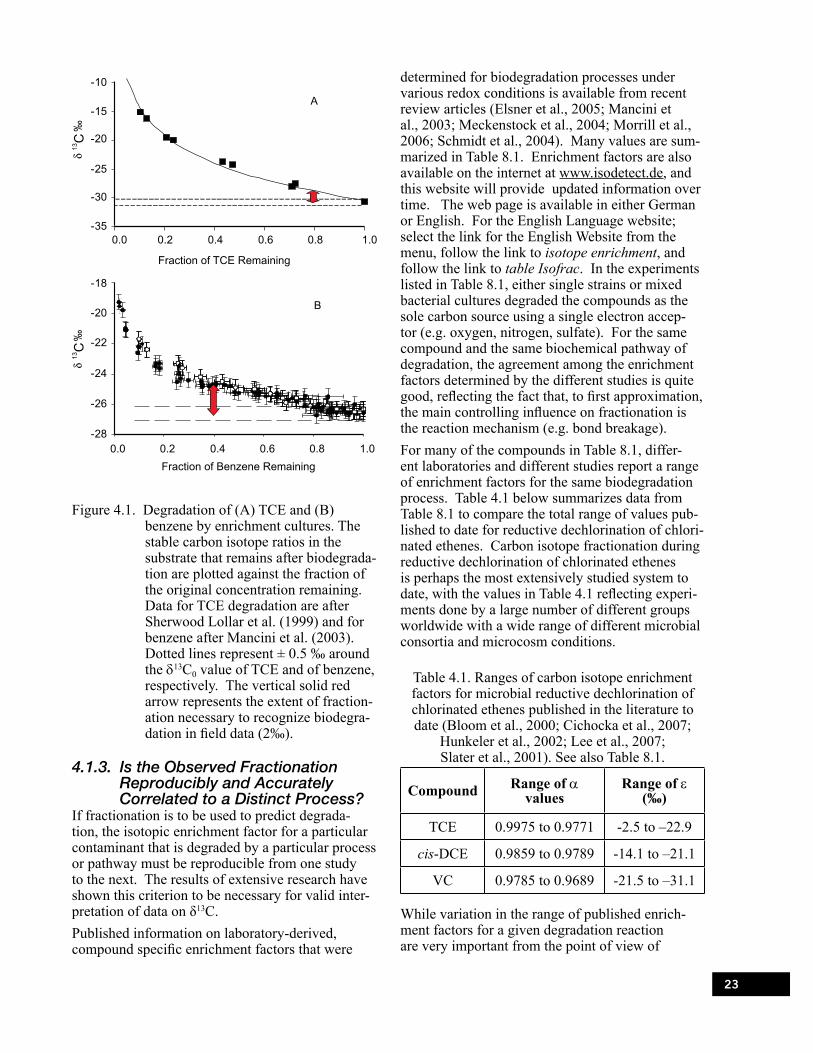
23

Figure 4.1. Degradation of (A) TCE and (B) benzene by enrichment cultures. The stable carbon isotope ratios in the substrate that remains after biodegrada-tion are plotted against the fraction of the original concentration remaining. Data for TCE degradation are after Sherwood Lollar et al. (1999) and for benzene after Mancini et al. (2003). Dotted lines represent ± 0.5 ‰ around the δ13C0 value of TCE and of benzene, respectively. The vertical solid red arrow represents the extent of fraction-ation necessary to recognize biodegra-dation in field data (2‰).

4.1.3. Is the Observed Fractionation Reproducibly and Accurately Correlated to a Distinct Process?

If fractionation is to be used to predict degrada-tion, the isotopic enrichment factor for a particular contaminant that is degraded by a particular process or pathway must be reproducible from one study to the next. The results of extensive research have shown this criterion to be necessary for valid inter-pretation of data on δ13C. Published information on laboratory-derived, compound specific enrichment factors that were

determined for biodegradation processes under various redox conditions is available from recent review articles (Elsner et al., 2005; Mancini et al., 2003; Meckenstock et al., 2004; Morrill et al., 2006; Schmidt et al., 2004). Many values are sum-marized in Table 8.1. Enrichment factors are also available on the internet at www.isodetect.de, and this website will provide updated information over time. The web page is available in either German or English. For the English Language website; select the link for the English Website from the menu, follow the link to isotope enrichment, and follow the link to table Isofrac. In the experiments listed in Table 8.1, either single strains or mixed bacterial cultures degraded the compounds as the sole carbon source using a single electron accep-tor (e.g. oxygen, nitrogen, sulfate). For the same compound and the same biochemical pathway of degradation, the agreement among the enrichment factors determined by the different studies is quite good, reflecting the fact that, to first approximation, the main controlling influence on fractionation is the reaction mechanism (e.g. bond breakage).For many of the compounds in Table 8.1, differ-ent laboratories and different studies report a range of enrichment factors for the same biodegradation process. Table 4.1 below summarizes data from Table 8.1 to compare the total range of values pub-lished to date for reductive dechlorination of chlori-nated ethenes. Carbon isotope fractionation during reductive dechlorination of chlorinated ethenes is perhaps the most extensively studied system to date, with the values in Table 4.1 reflecting experi-ments done by a large number of different groups worldwide with a wide range of different microbial consortia and microcosm conditions.

Table 4.1. Ranges of carbon isotope enrichment factors for microbial reductive dechlorination of chlorinated ethenes published in the literature to date (Bloom et al., 2000; Cichocka et al., 2007;

Hunkeler et al., 2002; Lee et al., 2007; Slater et al., 2001). See also Table 8.1.

Compound Range of a values

Range of e (‰)

TCE 0.9975 to 0.9771 -2.5 to –22.9

cis-DCE 0.9859 to 0.9789 -14.1 to –21.1

VC 0.9785 to 0.9689 -21.5 to –31.1

While variation in the range of published enrich-ment factors for a given degradation reaction are very important from the point of view of

24

understanding the details of the reaction mecha-nism, the variation in published values does not necessarily introduce a large uncertainty into the estimate of the fraction remaining after degradation (f) as calculated using Equation 4.2 or 4.3. For instance, the total analytical uncertainty in measured δ13C values is typically ± 0.5‰ for carbon CSIA for many of the hydrocarbon contaminants investigated to date. Total uncertainty in (f), the fraction of contaminant remaining, is at a mini-mum the analytical uncertainty associated with typical VOC concentration analyses. While under optimized performance, VOC concentrations can be determined to a precision of ± 5%; typically, commercial VOC analyses are ± 20 to 30%. In the estimate of (f) using Equation 4.2, uncertainty in the second or third decimal place in the exponent (a-1) does not contribute as much uncertainty as does the uncertainty in the direct calculation of (f) caused by uncertainty in the analysis of VOC con-centrations. This can be shown by calculating the propagation of errors for the individual parameters in the Rayleigh equation (Griebler et al., 2004b). More examples and discussion are provided in Section 4.2.3.4a.Data published to date suggests that the rate of bio-degradation does not seem to significantly impact the observed enrichment factor ε (Mancini et al., 2006; Morasch et al., 2001). The dominant con-trolling parameter on fractionation is the reaction mechanism. As is predicted from theoretical princi-ples of isotope fractionation, degradation pathways or reaction mechanisms can have characteristic sta-ble isotope enrichment factors based on the bonds that are broken. Variations between the stable isotope enrichment factors for one pathway com-pared to another are one of the most important fac-tors influencing stable isotope fractionation during biodegradation. This principle is a well-established foundation of stable isotope geochemistry, having been demonstrated for microbial methanogenesis via different pathways in a landmark paper in 1985 (Whiticar and Faber, 1985) and elucidated for photosynthesis by C3 versus C4 metabolic path-ways more than twenty years ago (O’Leary, 1981). It follows that conditions that control the dominant degradation pathway can control the characteristic fractionation pattern, and the value of the isotopic enrichment factor. For compounds that degrade under different reaction mechanisms under aero-bic versus anaerobic conditions, the characteristic isotopic fractionation observed varies with redox conditions. This has been quite extensively studied for MTBE (Hunkeler et al., 2001a; Kolhatkar et al., 2002; Kuder et al., 2002; Kuder et al., 2005; Rosell

et al., 2007; Zwank et al., 2005), benzene and tolu-ene (Ahad et al., 2000; Fischer et al., 2007; Fischer et al., 2008; Hunkeler et al., 2001b; Mancini et al., 2003; Mancini et al., 2008a; Meckenstock et al., 2004; Morasch et al., 2001; Morasch et al., 2002; Morasch et al., 2004) and is recently being eluci-dated for the chlorinated ethenes (Chartrand et al., 2005; Chu et al., 2004). Even under similar redox conditions, if different microbial populations use different degradation pathways, each can result in a reproducible and distinct value for the isotopic enrichment factor, as has been shown for aerobic biodegradation of 1,2-dichlorethane (Hirschorn et al., 2004), aerobic biodegradation of toluene (Morasch et al., 2002), and aerobic biodegradation of MTBE (Rosell et al., 2007). In most aerobic degradation pathways, the first step is usually an activation of the molecules by an oxy-genase reaction to introduce hydroxyl, epoxide or other reactive oxygen-containing groups. For some compounds, there are several types of oxygenase reactions, and the extent of isotope fractionation can depend on the particular oxygenase reaction that is responsible for biodegradation. In the case of aromatic hydrocarbons this may range from undetectable fractionation of stable isotopes of carbon for reactions that are carried out by dioxy-genase enzymes that attack the π-electron system of the aromatic ring to strong fractionation caused by reactions carried out by monooxygenase enzymes that attack the ring or methyl groups. Practical rec-ommendations for assessing the uncertainty intro-duced by the range of available fractionation factors are discussed in detail in Section 4.4.

4.1.4. Do Non-Degradative Processes Influence the Observed Isotope Fractionation?

In order to use CSIA to understand the degradation of contaminants, the isotope fractionation dur-ing degradation must be readily discernable from isotope effects associated with other subsurface processes that do not destroy the contaminant, such as volatilization, dissolution and sorption. Isotope fractionation during volatilization (Harrington et al., 1999; Ward et al., 2000); dissolution (Dempster et al., 1997; Hunkeler et al., 2004; Slater et al., 1999; Ward et al., 2000); diffusion (Hunkeler et al., 2004; Bouchard et al., 2008) and sorption (Harrington et al., 1999; Kopinke et al., 2005; Meckenstock et al., 1999; Schuth et al., 2003; Slater et al., 2000) is typically small or is indiscernible outside of the analytical uncertainty typical for CSIA (± 0.5‰ for carbon isotopes; ± 5‰ for hydrogen). During sorption of contaminants to carbonaceous material,

25

a hydrogen isotope shift of only 8‰ was observed after 95% of the contaminant was sorbed (Schuth et al., 2003). Significant hydrogen isotopic effects were only observed in laboratory experiments where aromatic hydrocarbons underwent near complete vaporization or sorption, in excess of 95% removal (Schuth et al., 2003; Wang and Huang, 2003). Hence, Wang and Huang (2003) noted that large isotopic shifts might be relevant to processes such as air sparging and to studies in the unsatu-rated zone, but large isotopic shifts are not likely to be significant in most natural systems where extensive mass loss due to volatilization or sorption is unusual. In a recent study documenting carbon isotope fractionation due to diffusion, Bouchard et al. (2008) demonstrated that even in the unsaturated zone where diffusive effects on isotope composi-tion might be expected to be most pronounced com-pared to the saturated zone, diffusive effects were only observable if measured within a few days of the spill, and where measurements could be done at a very fine spatial scale.

4.1.5. Do Abiotic Degradation Processes Occur and Produce Isotope Effects for the Compound of Interest?

The relative importance of biodegradation versus processes of abiotic degradation at the site must be considered. In the past few years, the principles of Rayleigh controlled isotope fractionation of organic contaminants in ground water have been shown to apply to abiotic degradation as well as biodegrada-tion (Bill et al., 2001; Elsner et al., 2007a; Elsner et al., 2008; Hofstetter et al., 2008; Slater et al., 2002; VanStone et al., 2004; VanStone et al., 2008; Zwank, et al., 2005). Zero valent iron is widely used in active remediation of ground water con-tamination. While much research is still underway to understand the precise reaction mechanisms associated with degradation of chlorinated eth-enes on zero valent iron, CSIA indicates that the mechanisms are similar to the familiar mechanisms associated with biodegradation, and that different abiotic degradation mechanisms are associated with different characteristic patterns of fractionation. Traditionally, rates of natural abiotic degradation in ground water were thought to be insignificant unless they were enhanced through abiotic reme-diation schemes such as the addition of zero valent iron. This view is changing. There have been several recent studies of the role of abiotic reac-tions with minerals and the role of microbially-mediated abiotic reactions at field sites (Bradley and Chapelle, 1997; Butler and Hayes, 1999;

Cervini-Silva et al., 2001; Ferrey et al., 2004; Lee and Batchelor, 2002; McCormick and Adrians, 2004). The possibility of abiotic degradation introduces the challenge of distinguishing between the effects of abiotic and biotic isotopic fractionation in any system where both types of degradation may be sig-nificant. Liang et al. (2007) noted that the isotope fractionation during abiotic degradation of PCE and TCE by FeS was much greater than the frac-tionation during anaerobic biodegradation of PCE and TCE. Reduced iron sulfides such as FeS can be an important component of aquifer sediments at hazardous waste sites. Liang et al. (2007) warn that the use of an enrichment factor appropriate for biodegradation instead of the factor appropriate for the abiotic mechanism may overestimate the true extent of degradation at field scale. A similar pat-tern of smaller biological enrichment factors com-pared to abiotically-mediated degradation has been identified for MTBE and 1,1,1-TCA (Elsner et al., 2007a; 2007b) and PCE (Lee et al., 2007; Nijenhuis et al., 2005; Slater et al., 2001; Slater et al., 2003), suggesting that additional rate-limiting factors in biochemical reactions require more in depth research. VanStone et al., (2008) and Elsner et al., (2008) discuss the potential of using CSIA to distin-guish between abiotic and biodegradation processes where both types of processes may be important.

4.1.6. Is the Rayleigh Equation an Appropriate Model to Describe the Data Set?

For compounds that are intermediates in degrada-tion pathways, such as the products of reductive dechlorination of chlorinated ethylenes, a straight-forward application of the Rayleigh equation (Equation 4.2) is not strictly possible. The isotope ratio in the intermediate compound will change due to the combined effects of isotopic fractionation during its production from the parent compound and isotopic fractionation due to its own continu-ing degradation. There is one important exception. The Rayleigh equation can be used when complete transformation of the parent compound occurs prior to further degradation of the intermediate com-pound (Morrill et al., 2005). When production and degradation of the interme-diate compound occurs simultaneously, a more complex isotope evolution occurs that can be evaluated using multistep reactive transport models (van Breukelen et al., 2005; Morrill et al., 2006). Quantitative information on biodegradation can be obtained by fitting an analytical model (Beranger et al., 2005) or numerical model (van Breukelen,

26

et al., 2005) that describes the isotope evolution during sequential processes to the measured isotope data. Van Breukelen et al. (2005) used a simple one dimensional model to provide insight in the rates of transformation of parent and intermediate compounds. The simulation of different degrada-tion scenarios such as various degrees of degrada-tion or different relative rates of biodegradation for different steps in a multi-step process can also be very useful as a benchmark for a semi-quantitative interpretation of isotope data.For certain chlorinated solvents the situation is even more complex because the degradation pathways of different compounds can converge and produce the same daughter products (Kirtland et al., 2003). For example, trichloroethylene (TCE) can be produced from biological reductive dechlorination of tetra-chlorethylene (PCE), or through an abiotic reaction from 1,1,2,2-tetrachlorethane. If several potential parent compounds are present in ground water at the same time, it is difficult to interpret the behav-iour of the compound from CSIA. Due to these complexities, the conceptual model for biodegrada-tion at a site should distinguish those compounds that are only present as parent compounds from those compounds which might be present both as parent and daughter compounds. See for example Hirschorn et al., (2007). Section 4.2 covers the appropriateness of a Rayleigh model in more detail with respect to field data.

4.2. Recommended Steps for the Quantification of Biodegradation Based on CSIA

4.2.1. Site Characterization Use of CSIA is no silver bullet and will be most useful and cost effective when applied within the context of the hydrological, geological, geochemi-cal and microbiological parameters at the site. The factors that affect contaminant transport and degra-dation over time as well as space must be identified and evaluated. This includes the important geohy-drological parameters (ground water flow direction, hydraulic conductivity, hydraulic gradient) and geochemical conditions (concentrations of oxygen, nitrate or sulfate within the plume). Ultimately, a conceptual site model can be developed that will reveal practicable remediation goals that are capable of protecting existing or potential recep-tors from contamination. Iterative generation and interpretation of field data from a general survey is necessary to identify the major compartments of the plume (the source, the fringe, the center line, and the mixing zones) as well as the most relevant processes that contribute to natural attenuation.

4.2.2. Evaluate Field Data for the Fit to the Rayleigh Model

The Rayleigh model (Equation 4.2 and 4.2) predicts that a plot of δ13C or δ2H on the logarithm of the concentration remaining should be a straight line. If field data are plotted as described above, and the data follow a straight line, then a single process for biodegradation or abiotic transformation likely con-trols the concentrations at field scale, as illustrated in Figure 4.2. This is called a Rayleigh correlation. Dilution, dispersion, sorption, volatilization, and mixing between contaminant sources with different values of δ13C or δ2H will cause the data to fall off of the straight line. Given the importance of dilution and dispersion at field scale, it might intuitively seem likely that no set of realistic field data would show a Rayleigh correlation. However, case studies and evolving field experience have in fact shown that a signifi -fact shown that a signifi - shown that a signifi-cant number of sites do have field data that fit the Rayleigh model (Abe and Hunkeler, 2006; Griebler et al., 2004b; Kolhatkar et al., 2002; Morrill et al., 2005). The existence of such a correlation indicates that biodegradation or abiotic transformation is the significant process that controls changes in concen-trations of contaminants.

Figure 4.2. Testing field data on CSIA and concen-trations of contaminants for fit to the Rayleigh equation. Deviations from a straight regression line in the plot of δ13C on the natural logarithm of con-centration can indicate that processes other than degradation control the con-centrations of contaminants. Example data plotted for Table 1 of Kolhatkar et al. (2002). The dotted lines bound the values of δ13C that are expected for MTBE that was blended into gasoline.

27

The first recommendation for using CSIA to quantify biodegradation is to plot the δ13C of the compound against the natural logarithm of the concentration of the compound to determine if these parameters show a Rayleigh correlation as illustrated in Figure 4.2. This “test” is simply the first step in determining if the Rayleigh controlled fractionation inherent in Equation 4.2 is an appro-priate model for the site. There is no need to take the location of the respective wells into account on this level when performing the Rayleigh analysis because the location does not influence the calcula-tion. However, data points that drastically fall of the straight regression line can be identified and might be evaluated further for other processes that influ-ence the compound apart from biodegradation, such as dilution in the monitoring well, dispersion along the flow path, or volatilization. A strong correlation to the Rayleigh model adds considerable confidence to the application of CSIA data to understand the behaviour of a contaminant at a site. Variations in the length and elevation of the screened interval of monitoring wells can cause a well to produce ground water that is either domi-nated by the plume of contamination, or cause the well to produce water that has a small contribution from the plume and a major contribution from clean ground water above or below the plume. Details of well construction can have a strong effect on the concentration of the organic compound in water produced by the well. A poor correlation to the Rayleigh model may be due to these incidental perturbations in the concentration that are created by the monitoring wells. As a result, a poor cor-relation does not automatically disqualify a site for the application of CSIA to understand the transfor-mation processes.

4.2.3. Determination of the Primary Isotope Signature (δ13Csource or δ2Hsource )

The primary isotopic signature is the isotopic ratio of the organic contaminant of concern before it is fractionated by biodegradation processes or abiotic transformations. The ideal approach would be to measure the isotopic signature of the primary con-taminant that was spilled at the site. However, this is rarely feasible. Nor is measurement of δ13Csource or δ2Hsource for the most recent spill necessarily rel-evant at many sites where there has been a history of multiple spills or leakage. There are three basic approaches to determination of δ13Csource or δ2Hsource. One approach compares values of δ13C or δ2H for contaminants in ground water to values of δ13C or δ2H reported in the

literature. The second and third approaches are entirely site specific. They compare δ13C or δ2H for contaminants in different samples of ground water to determine the extent of degradation between points in space (between different wells) or points in time (temporal variation within a single well) at a specific site.

4.2.3.1. Value of δ13Csource or δ2Hsource Based on Literature.

In the routine case where samples of the actual spilled material are neither available nor relevant, the approach is to make an assumption for δ13Csource or δ2Hsource based on published values in the lit-erature for undegraded pure product. This is not unreasonable for petroleum hydrocarbons, or for anthropogenic compounds such as chlorinated ethenes produced from petroleum hydrocarbon feedstocks, because the range of δ13C for petroleum hydrocarbons is well characterized and relatively well constrained. As degradation proceeds, a point is reached where the value of δ13C or δ2H may be more positive (more enriched in 13C or 2H) than any reported value from commercially available products. When the value of δ13C or δ2H in the field is more positive than the range in the pure sub-stance, degradation at the site is evident (compare Figure 4.2).

4.2.3.2. Values of δ13Csource or δ2Hsource Based on Most Negative Value at the Site

Because biodegradation induces a shift of the residual compound to less negative values of δ13C or δ2H, the most negative values measured for the organic contaminant in ground water at the site can be the best estimate of the original values of δ13Csource or δ2Hsource. While this approach can work well for compounds for which the fractionation due to biodegradation is large (tens of ‰) relative to the variation in assumed δ13Csource , the approach is not recommended for compounds such as benzene and toluene for which the error in the assumption of δ13Csource will be large with respect to a relatively small changes in δ13C caused by biodegradation.

4.2.3.3. Values of δ13Csource or δ2Hsource Based on Point to Point or Time to Time Comparisons

Quantifying the relative amount of biodegradation between wells, or in a given well over time, is com-pelling since it involves fewer assumptions than the literature-based approach. It does, however, require a good hydrogeological and geological understand-ing of the site. In this approach, one can select wells for δ13Csource or δ2Hsource that sample the known

28

source zone. As an example, the wells might be screened across an interval with non aqueous phase liquids (NAPL) that act as the source of ground water contaminant. Wells in the source area would be expected to produce water with the highest con-centrations of contaminants. Since biodegradation produces more enriched (less negative) δ13C values, such wells may be assumed to represent the least degraded material at the site. It is important to note that this approach will pro-vide a conservative estimate of the extent of bio-degradation. If undegraded compound is in fact being added to the plume through mixing, desorp-tion, or continued dissolution of NAPL, the addi-tion of this more isotopically negative δ13C material will minimize the observed fractionation effects produced by biodegradation (Abe and Hunkeler, 2006, Morrill et al., 2005). While continued dis-solution of NAPL close to the source zone may result in a complete suppression of the fractionation signal of biodegradation, the calculation can at least provide a conservative upper boundary on C/Co. The true fraction remaining may be less than the estimate.The most thorough approach would be to calcu-late the extent of biodegradation using all three approaches for determining δ13Csource. If the three estimates agree, the extent of biodegradation is well constrained. In several case studies this was indeed the situation because the source well δ13C values were not only the most negative δ13C values at the site, but they were within the published range for undegraded pure product (Sherwood Lollar et al., 2001).

4.2.3.4. Selection of an Appropriate Enrichment Factor

This Guide assumes that the isotope enrichment factors derived from laboratory microcosm studies are applicable to the field. In contaminant hydrol-ogy, the removal of organic contaminants in tradi-tional laboratory microcosm studies is commonly used to predict the removal in field scale plumes. The assumptions made in extrapolating isotope enrichment factors to the field are equivalent to the assumptions made in extrapolating data on con-taminant degradation from laboratory microcosm studies to predict the behaviour of a plume at field scale.As discussed in Section 4.1.3, there are two important sources of uncertainty in extrapolation of enrichment factors. The value of the enrich-ment factor is sensitive to the biodegradation pathway (and hence to parameters such as redox conditions and microbial populations) and to the

reproducibility of fractionation factors under any given set of conditions for any given biodegrada-tion reaction pathway. The selection and evalua-tion of enrichment factors from the literature is a two step process. First, use site specific data on geochemical parameters to determine the most probable pathway for metabolism (or abiotic trans-formation) of the contaminant at field scale. Then search the literature (Table 8.1) for published enrichment factors for the compound of interest under the relevant redox conditions. The variation in published enrichment factors for a given set of conditions is a measure of the repro-re of the repro-ducibility of the enrichment factor. One option to deal with the variation in published enrichment factors is to select the largest enrichment factor in the literature to estimate the extent of biodegrada-tion at field scale. In this case, the “largest” enrich-ment factor is the most negative factor, the factor with the largest absolute value. For a given change in the value of δ13C or δ2H, the largest enrichment factor will predict the largest value for the fraction remaining after biodegradation and will predict the smallest extent of biodegradation. As a result, the largest value for the enrichment factors will provide the most conservative estimate of the extent of bio-degradation. When the difference in values of δ13C between the source and the down gradient monitor-ing wells is small (2‰ to 5‰), the value selected for the enrichment factor can have a stronger influ-ence on the extent of biodegradation predicted from Equation 4.3. A second option to deal with variation in the published values of the enrichment factors is to calculate a lower boundary on the extent of bio-degradation using the highest published enrich-ment factor, an upper boundary using the lowest published enrichment factor, and a best estimate of bioremediation using the mean of all the enrich-ment factors, then compare the predictions of the extent of bioremediation. When this approach was applied to data from studies of bioremediation of TCE and cis-DCE at spill sites at Dover Air Force Base in Dover, Delaware, USA and at Kelly Air Force Base in San Antonio, Texas, USA, the differ-ence between the upper and lower boundaries on the extent of biodegradation was small (Morrill et al., 2005, Sherwood Lollar et al., 2001). A third option is to calculate the mean and the standard deviation of the enrichment factors, and then use statistical techniques to estimate propaga-tion of error to determine the effect of the variation in published values for the enrichment factor on the estimate of the extent of biodegradation.

29

Reactions with large fractionation factors (e more than an absolute value of 3‰) allow a more sensi-tive quantification of biodegradation, while reac-tions with small fractionation factors (e smaller than an absolute value of 1‰) require a large degree of biodegradation (>90%) before a signifi-cant isotopic difference between source and moni-toring wells can be resolved (Ahad et al., 2000). As a general principle, as the difference between δ13C and δ13Csource becomes larger, the uncertainty in the calculation of the extent of biodegradation becomes smaller. Figure 4.3 compares the relative effect of the value of the isotopic enrichment factor, and the value of δ13Csource, on the predicted extent of biodegrada-tion. When the value of δ13C is close to the value of δ13Csource, the estimate of the extent of biodegrada-tion is more sensitive to the value of δ13C. When the value of δ13C is further away from the value of δ13Csource, the estimate of the extent of biodegrada-tion is more sensitive to the value of the enrichment factor ε. One may be tempted to use fractionation data from a contaminated field site to determine implicit iso-tope enrichment factors. Although some scientific studies have practiced this approach (Steinbach et al., 2004), it cannot be recommended as a general procedure. The complexity of hydrogeological and microbial processes in the field will give only a crude estimate of the enrichment factor com-pared to well-controlled laboratory experiments and will certainly introduce additional uncertainty. Therefore, it is advisable to take appropriate labora-tory-derived enrichment factors from the literature.

Figure 4.3. Relative influence of different values for δ13Csource (Panel A) and different values for the isotopic enrichment fac-tor ε (Panel B) on the calculated extent of toluene biodegradation. The extent of biodegradation is expressed in per-cent of the material originally present, calculated as B = (1-f ), where f is the fraction remaining as calculated from Equation 4.3. The dashed lines are es-timates of the extent of biodegradation from δ13C for biodegradation of toluene under methanogenic conditions where e = -0.5‰ with two different values for δ13Csource. The solid line is an estimate of the extent of biodegradation under sulfate-reducing conditions where e = -1.5‰.

4.2.3.5. Estimating an Enrichment Factor when none is Available.

Although the literature on isotope enrichment fac-tors is expanding rapidly, there may be occasions when an isotopic enrichment factor for a particular compound is not available in the literature. The following material describes an approach that may be used to estimate an isotopic enrichment factor from the data available for similar compounds.Stable isotopic fractionation occurs at a distinct chemical bond within a molecule, where the

enzymatic reaction takes place. A heavy isotope at an adjacent position might still affect the reaction but to a much lower extent (referred to as a second-ary isotope effect) and can usually be neglected. Heavy atoms further distant from the reactive posi-tion have no influence on isotope fractionation. As a first approximation, only the atom in the reactive position of the molecule undergoes isotope frac-tionation. However, in CSIA the isotopic composi-tion of all of the atoms of a respective element in the molecule is measured (e.g. all carbon atoms).

30

The stable isotope effect is therefore “diluted” by the number of atoms at non-reactive positions of a compound. One can distinguish between the intrin-sic isotope enrichment factor (εi ) which considers only the isotope shifts at the reactive position and the overall isotope enrichment factor (ε) which determines the isotope fractionation of the entire molecule. Details of this approach can be found in Elsner et al. (2005) and Morasch et al. (2004). The relation of (ei ) and (e) follows Equation 4.5, where (n) is the total number of atoms of a particular ele-ment in the molecule.

/niε = ε 4.5

From the stable isotope enrichment factors and the intrinsic factors published for anaerobic or aerobic degradation of mineral oil constituents and chlori-nated solvents it is apparent that CSIA can be suc-cessfully applied to recognize isotope fractionation in compounds with no more than twelve to thirteen carbon atoms. For larger molecules, the expected isotope shifts will be so strongly diluted that they fall into the range of the experimental error of the isotope analysis (Morasch et al., 2004). Expressing fractionation as the intrinsic enrichment factor (εi) reveals that the same biochemical reac-tions produce similar intrinsic enrichment factors for different compounds. Anaerobic degradation of BTEX compounds and methylnaphthalene provide a good example. The primary enzyme reaction in the anaerobic degradation pathways of methylated aromatic hydrocarbons (toluene, xylene, methyl-naphthalene) is always a fumarate addition to the methyl group by glycyl radical enzymes. The intrinsic carbon isotope enrichment factors have been shown to be similar (Morasch et al., 2004). If there is no published value for the isotope enrich-ment factor (ε) for a compound, but the biochemi-cal reaction of the primary degradation step is known, it should be possible to use literature values for the intrinsic enrichment factors (εi) of similar compounds to estimate an isotope enrichment fac-tor (ε) for the compound. Such estimates have been shown to be in the same range of accuracy as those obtained from laboratory experiments with the respective compounds (Meckenstock et al., 2004; Morasch et al., 2004; Zwank et al., 2005).As an example, a representative carbon isotope enrichment factor for toluene which can be taken from the literature is -1.7‰. As toluene contains 7 carbon atoms the intrinsic enrichment factor ei for the reactive carbon position is -1.7‰ * 7 = -11.9‰ (Table 8.1). Imagine that we require an enrichment factor for xylene. Because the initial reaction of

the degradation pathway of xylene is similar to toluene degradation we will make an assumption that the intrinsic enrichment factor ei for xylene is the same as for toluene (ei = -11.9‰). For the overall enrichment factor e we divide the esti-mate of ei by 8 (xylene contains 8 carbon atoms) to produce an estimate for the enrichment factor of -11.9‰ / 8 = - 1.5‰. This estimate is exactly equivalent to the only value that is available in the literature for a pure culture study of the anaerobic biodegradation of xylene (Morasch et al., 2004; Table 8.1). However, Table 8.1 also reveals that the variation of fractionation factors determined for anaerobic xylene degradation is quite large.

4.2.3.6. Concurrent Application of CSIA Analysis for Different Elements (Two-Dimensional Analysis).

For some contaminants, such as MTBE and ben-zene, there is a fundamental difference in the enzymatic mechanism for biodegradation under aerobic and anaerobic conditions, and the differ-ence in enzymatic mechanism is reflected in a large difference in the values of the enrichment factors (e) under aerobic or anaerobic conditions. As discussed in Section 4.1.5 and Section 4.2.3.4, depending on the compound, different values of e may have an effect on the predicted extent of bio-degradation, and the implications should be investi-gated as in the example in Figure 4.3. If field measurements of δ13C are to be used to estimate the extent of degradation, it is necessary to know the mechanism of degradation to be able to select the correct value of ε. Frequently it is not possible from conventional site characteriza-tion data to unequivocally associate biodegradation with either the aerobic mechanism or the anaerobic mechanism. However, it may be possible to iden-tify the mechanism of degradation from the con-current enrichment of both carbon and hydrogen isotopes. Kuder et al. (2005) compared the enrich-ment of carbon and hydrogen during biodegrada-tion of MTBE in anaerobic microcosms and in field samples from gasoline spill sites in the USA. In a plot of δ2H for MTBE against δ13C for MTBE, the data from the field sites had the same distribution as the distribution of the data from the anaerobic microcosm study (Figure 4.4). Zwank et al. (2005) made the same comparisons of δ2H against δ13C for MTBE contamination in ground water at a former industrial landfill in South America, and established that MTBE degraded under anaerobic conditions at that site as well. Zwank et al. (2005) applied the term “two-dimen-sional analysis” to describe the concurrent CSIA

31

for both carbon and hydrogen, and offered the approach as a useful tool to distinguish the pathway of biodegradation of MTBE in ground water at field scale.The dotted line in Figure 4.4 projects the values of δ2H and δ13C for MTBE that would be expected from values of eC of -2.4‰ and eH of -30‰. These values are the extremes in the range reported in Gray et al. (2002) for aerobic biodegradation of MTBE by strain PM1 or mixed cultures that resembled PM1 in their behavior. These organisms degrade MTBE by oxidation of the methyl group with an oxygenase enzyme. Because oxygenase enzymes act by extracting a proton from the methyl group, there is a very strong enrichment of deute-rium in the residual MTBE. To provide the most conservative estimate in Figure 4.4, the projections of δ2H and δ13C expected in MTBE in ground water start from the most positive values of δ2H and δ13C determined in MTBE in gasoline as reported in Kuder et al. (2005). The actual distribution of δ2H against δ13C for MTBE at field scale was very different than the distribution that would be expected from aerobic biodegradation of MTBE. The actual distribution of δ2H corresponds to εH of -11.5‰. Zwank et al. (2005) reported an estimate of eH of -15.6‰ at the site in South America. The actual distribution

of δ13C corresponds to a value of eC in the range -8.9‰ to -10.2‰. The first step in anaerobic biodegradation of MTBE is hydrolysis of the ether bond (Kuder et al., 2005; Zwank et al., 2005). In the hydrolysis reaction, there is strong enrichment of 13C in the carbon atoms involved in the ether bond. Because the hydrogen atoms are not directly involved, there is much less fractionation of hydrogen. Rosell et al. (2007) compared the distribution of δ2H against δ13C for MTBE during aerobic deg-radation by two cultures that metabolized MTBE through a different pathway that involves attack on the ether bond. The value of εH was -0.2‰ for strain L108 and +5‰ for strain IFP2001. In these organisms, the values of eH are much lower than is the case for organisms like PM1. Enrichment of δ2H and δ13C during aerobic biodegradation by these organisms is projected as the solid line in Figure 4.4. The values used in the projection were eC of -1.48‰ and eH of -0.2‰. There was considerable overlap of the field data of Kuder et al. (2005) and plausible values of δ2H and δ13C that would be expected from aerobic biodegradation of MTBE by organisms similar to strains L108 and IFP2001. As a consequence, Rosell et al. (2007) warn against uncritical comparison of δ2H and δ13C

Figure 4.4. Concurrent analysis of δ13C in MTBE and δ2H in MTBE in ground water to associate natural biodegradation of MTBE in ground water with an anaerobic process, which allows the selec-tion of an appropriate value for the enrichment factor (ε) to be used to estimate the extent of biodegradation of MTBE.

32

in MTBE in the field to infer the primary pathway for biodegradation. The length of the solid line in Figure 2.4 is the range of values of δ2H and δ13C that would be expected in MTBE when MTBE is degraded from an initial high concentration of 100,000 µg/L to 1 µg/L. Only 5% of gasoline spill sites in the USA have initial concentrations of MTBE above 100,000 µg/L, and 1 µg/L is the lower limit for determination of δ2H and δ13C in MTBE in water samples. The solid line in Figure 4.4 represents the plausible range of δ2H and δ13C that would be expected during aerobic biodegradation of MTBE by organisms similar to strains L108 and IFP2001. By examination of Figure 4.4, and allowing for uncertainty in the estimation of δ2H of 10‰ and δ13C of 0.5‰, the two dimensional approach pro-posed by Zwank et al. (2005) can be used to distin-guish anaerobic biodegradation of MTBE whenever the value of δ2H in MTBE in the field sample is more positive than -67‰ and δ13C is more positive than -9‰.Similar success has been reported recently for determining benzene biodegradation pathways (Fischer et al., 2007; Fischer et al., 2008; Mancini et al., 2008a). The approach will find wider use, and have more validity, as more data are available on the concurrent enrichment of δ2H and δ13C in organic contaminants by different microorganisms under different geochemical conditions.

4.3. Conversion of Calculated Extent of Biodegradation (1-f ) to Biodegradation Rates

At many hazardous waste sites, mathematical models are used to predict the transport of contami-nants in ground water from source areas to potential receptors such as drinking water wells. These models are calibrated using estimates of the rate of biodegradation of the contaminant in ground water. Most commonly the rates of biodegradation are extracted from field monitoring data. These con-ventional approaches compare changes in concen-tration of the contaminant with travel time along a flow path in an aquifer. One valuable application of CSIA is an independ-ent evaluation of the rates of biodegradation of contaminants. Section 7.3 derives equations that can be used to calculate the rates of biodegrada-rates of biodegrada-tion or abiotic transformation at field scale from an estimate of the fraction remaining after biodegrada-tion (C/Co) and from some assumptions about flow paths and ground water flow rates for the site. This approach combines the uncertainty in the estimates

of the hydrogeological parameters with any uncer-tainties in the estimate of the extent of biodegrada-tion based on CSIA and Equation 4.3. Nonetheless, several recent case studies have shown good agree-ment between biodegradation rates extracted from isotope studies and rates derived by conventional approaches that are based on changes in concentra-tions in monitoring wells along a flow path in the aquifer (van Breukelen et al., 2005; Fischer et al., 2006; Hirschorn et al., 2007; Morrill et al., 2005). A key point to emphasize is that CSIA typically provides a more conservative estimate of the degra-dation rate compared to the conventional approach (Abe and Hunkeler, 2006; Chartrand et al., 2005; Morrill et al., 2005).

4.4. Using Estimates of Rates of Biodegradation to Predict Plume Behaviour

In the conventional approach, the extent of removal along a flow path is estimated by dividing the concentration of contaminant in a down gradient well (Ct) by the concentration in an up gradient well (C0). Often at field scale, monitoring wells are screened vertically across plumes, and produce samples of the contaminated plume that are diluted with clean water from above or below the plume. Occasionally a well will only sample the top or bottom of a plume. In this case the apparent attenu-ation of concentrations of contaminants has a strong component of dilution, and data on concentrations cannot be used in the conventional approaches to estimate the extent of removal. Fischer et al. (2006) provided an approach for solving this problem by taking the concentration that is actually measured in the down gradient well Ct and the measured values of δ13C in the two wells, to calculate a theoretical value for C0 using the Rayleigh equation. The difference between the calculated theoretical value of C0 and the measured value of Ct provides an estimate of the amount of compound that was degraded that is independent of dilution or other non destructive processes that can lead to a reduction of the contaminant concentra-tion (Fischer et al., 2006). Because the estimate of the extent of biodegradation provided by CSIA is independent of the concentration of the contaminant in the ground water sample, the extent of biodeg-radation from the CSIA analyses and the estimated travel time from the source of contaminant to a well can be used to estimate the rate of biodegradation along the flow path. The behaviour of contaminants in most plumes is heterogeneous, with extensive biodegradation

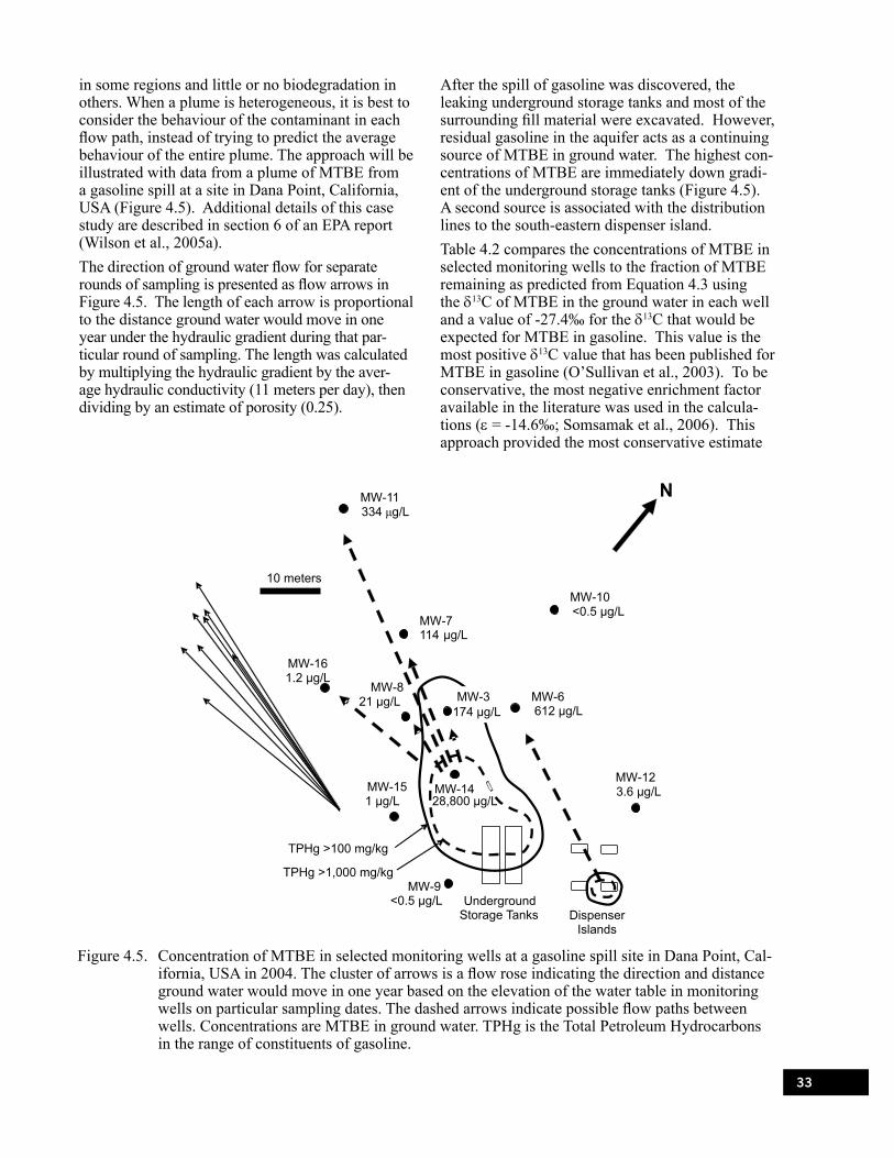
33

Figure 4.5. Concentration of MTBE in selected monitoring wells at a gasoline spill site in Dana Point, Cal-ifornia, USA in 2004. The cluster of arrows is a flow rose indicating the direction and distance ground water would move in one year based on the elevation of the water table in monitoring wells on particular sampling dates. The dashed arrows indicate possible flow paths between wells. Concentrations are MTBE in ground water. TPHg is the Total Petroleum Hydrocarbons in the range of constituents of gasoline.

in some regions and little or no biodegradation in others. When a plume is heterogeneous, it is best to consider the behaviour of the contaminant in each flow path, instead of trying to predict the average behaviour of the entire plume. The approach will be illustrated with data from a plume of MTBE from a gasoline spill at a site in Dana Point, California, USA (Figure 4.5). Additional details of this case study are described in section 6 of an EPA report (Wilson et al., 2005a).The direction of ground water flow for separate rounds of sampling is presented as flow arrows in Figure 4.5. The length of each arrow is proportional to the distance ground water would move in one year under the hydraulic gradient during that par-ticular round of sampling. The length was calculated by multiplying the hydraulic gradient by the aver-age hydraulic conductivity (11 meters per day), then dividing by an estimate of porosity (0.25).

After the spill of gasoline was discovered, the leaking underground storage tanks and most of the surrounding fill material were excavated. However, residual gasoline in the aquifer acts as a continuing source of MTBE in ground water. The highest con-centrations of MTBE are immediately down gradi-ent of the underground storage tanks (Figure 4.5). A second source is associated with the distribution lines to the south-eastern dispenser island. Table 4.2 compares the concentrations of MTBE in selected monitoring wells to the fraction of MTBE remaining as predicted from Equation 4.3 using the δ13C of MTBE in the ground water in each well and a value of -27.4‰ for the δ13C that would be expected for MTBE in gasoline. This value is the most positive δ13C value that has been published for MTBE in gasoline (O’Sullivan et al., 2003). To be conservative, the most negative enrichment factor available in the literature was used in the calcula-tions (e = -14.6‰; Somsamak et al., 2006). This approach provided the most conservative estimate

34

of the fraction of MTBE remaining compared to the MTBE that was originally present in the gasoline spilled to the aquifer.Table 4.2 reveals that the most conservative approach to calculate C/Co must have underesti-mated the true extent of biodegradation at this site. Well MW-11 had a value of δ13C for MTBE that was even more negative than the value assumed for MTBE in the gasoline that was spilled. The true value of δ13C for MTBE in the gasoline that was spilled may have been even more negative than -28.9‰. This most conservative approach was taken because this study was conducted as part of a risk evaluation, and the rates extracted from the CSIA analyses were the only rates available. If the purpose of the study were to validate other rates of biodegradation that were extracted from conven-tional approaches, it would have been appropriate to use estimates of δ13Csource that were more likely to be representative of the true δ13Csource. The most contaminated well at the site (MW-14 in Figure 4.5) is located in an area that had 9,000 mg/kg of Total Petroleum Hydrocarbons in the range of constituents of gasoline (TPHg). Wells MW-3 and MW-8 are further down gradient of the source of MTBE associated with the underground storage tanks (Figure 4.5). The δ13C of MTBE in wells MW-3 and MW-8 is much more enriched in 13C than MTBE in gasoline with values of +8.5‰ and +38.0‰ respectively. The fraction remain-ing corresponds to 91% and 99% biodegradation

of MTBE. The attenuation in concentration of MTBE in wells MW-3 and MW-8 compared to well MW-14 can be attributed to biodegradation. Well MW-6 appears to be cross gradient to the source of MTBE associated with the under-ground storage tanks (compare the flow arrows in Figure 4.5). However, well MW-6 is directly down gradient of the secondary source associated with the dispenser islands. The behaviour of MTBE in well MW-6 is very similar to wells MW-3 and MW-8. The δ13C of MTBE (-1.6‰) is highly enriched relative to MTBE in gasoline, and the predicted fraction remaining corresponds to 83% biodegradation of MTBE.Wells MW-7 and MW-11 are even further down gradient of the source of MTBE. The concentra-tions of MTBE are low, and it would be tempting to attribute the low concentrations to biodegradation. However, the δ13C of MTBE in these wells is even more depleted in 13C (-27.3‰, -28.9‰) than the δ13C in MW-14, the most contaminated well. The δ13C of MTBE in these wells falls near or within the range of δ13C expected for MTBE in gasoline. Hence, there is no evidence from the δ13C of MTBE that biodegradation contributed to attenuation of MTBE in these two down gradient wells. Because the isotope fractionation provides a direct estimate of the fraction of contaminant remaining after biodegradation, the rate constant for bio-degradation can be calculated from the removal

Table 4.2. Rates of natural biodegradation of MTBE in ground water moving along a flow path to monitor-ing wells. The rates were calculated from the estimated seepage velocity of ground water and the fraction of

MTBE remaining after biodegradation.

Well MTBE (μg/L)

δ13CMTBE

(‰)

Fraction MTBE

Remaining (C/Co)

Distance from MW-14 (meters)

Rate of Degradation with Distance (per meter)

Rate of Degradation

with Time (per year)

MW-14 28,800 -21.6 0.67 0MW-3 174 8.5 0.085 9.6 0.26 9.4MW-8 21 38.0 0.0113 11.7 0.38 14.1MW-7 114 -27.3 0.995 23.0 0.00021 0.0077MW11 334 -28.9 1.11 44.1 0 0

Distance from Dispenser Island

(meters)MW-6 612 -1.6 0.171 31.1 0.057 2.1

35

of contaminant along the flow path in the aquifer, the distance between wells, and an estimate of the interstitial seepage velocity. If biodegradation fol-lows a pseudo first order rate law, the rate of attenu-ation can be expressed directly as a first order rate of attenuation with distance, or the rate of attenua-tion with distance can be multiplied by an estimate of the seepage velocity of ground water to calculate a rate of attenuation with time of travel. The rate of attenuation with distance is calculated follow-ing Equation 4.6. Attenuation with time follows Equation 4.7.

( )with distance ln /f dλ = − 4.6

( )with time ln * /f v dλ = − 4.7

In Equation 4.6 and 4.5, λ is the rate of natural biodegradation, f is the fraction of contaminant remaining predicted from Equation 4.3, d is the distance along the flow path between the up gradi-ent well and the down gradient well, and v is the ground water seepage velocity.The average hydraulic conductivity at the site in Dana Point, California is 11 meters per day. The average hydraulic gradient over eight rounds of sampling was 0.0023 meter per meter. Assuming the effective porosity is 0.25, the average ground water seepage velocity should be near 37 meters per year. Table 4.2 presents the rates of biodeg-radation of MTBE along flow paths between the most contaminated well (MW-14), and down gradi-ent wells MW-3, MW-7, MW-8, and MW-11, and between the secondary source at the pump island and down gradient well MW-6. In wells MW-3 and MW-8, the first order rate of degradation is rapid, on the order of 0.3 per meter of travel, or 10 per year of residence time. In well MW-6, the rate of biodegradation is about ten fold slower. In well MW-7, the rate of biodegradation was one thousand fold slower, and in well MW-11 biodegradation was not detected at all. The field rates estimated for wells MW-3, MW-6 and MW-8 are in good agreement with laboratory rates reported in the literature. The rate of anaero-bic biodegradation of MTBE in a microcosm study constructed with material from a gasoline spill in Parsippany, New Jersey, varied from 11 ± 2.3 per year to 12 ± 2.9 per year (Wilson et al., 2005b). The rate of anaerobic MTBE biodegradation in a microcosms study constructed with core mate-rial from a JP-4 jet fuel spill in Elizabeth City, North Carolina, was 3.02 ± 0.52 per year and 3.5 ± 0.65 per year (Wilson et al., 2000).

The distance travelled before the concentration of contaminant reaches a particular goal (dfurther) can be calculated by rearranging Equation 4.7 to produce Equation 4.8. In Equation 4.8, F is the ratio of the goal to the existing concentration in the monitoring well.

further with distanceln( ) /d F= − λ 4.8

If F is calculated by dividing the U.S. EPA advisory limit of 20 μg/L by the concentration of MTBE remaining in monitoring wells MW-3, MW-6, or MW-8 (Table 4.2), and if the fi rst order rates of bio- rst order rates of bio-degradation also apply to the flow path that is down gradient of the monitoring wells, then the plume would move 8.4 meters past MW-3, and 60 meters past MW-6. Biodegradation had essentially already brought the concentration of MTBE to the limit in well MW-8. In contrast, the first order rate of biodegradation in well MW-7 (Table 4.2) is much slower. At a rate of 0.00021 per meter, starting at a concentration of 114 µg/L, the MTBE plume would be expected to move 8,300 meters further down gradient before it reached the advisory limit of 20 μg/L. In well MW-11, biodegradation of MTBE could not be established based on the δ13C for MTBE in the ground water. The concentration of dissolved oxygen in water from well MW-1 was 0.65 mg/L, the concentration of Iron(II) was 0.2 mg/L, and the concentration of methane was 0.018 mg/L. Conditions were not favourable for aerobic biodeg-radation. The only processes that can be reasonably expected to attenuate MTBE further down gradient of MW-11 are dilution and dispersion. It would appear that while the biodegradation of MTBE in the core of the plume was rapid and extensive, MTBE in the periphery of the plume was not degraded. As a consequence of the spatial heterogeneity in the rate of biodegradation, the extent of the plume would be seriously underestimated if a single rate constant for biodegradation was applied to the maximum concentration of MTBE in the source area. On the other hand, the maximum extent of the plume was seriously overestimated if biodegra-dation was ignored. At this point in the evolution of risk evaluation, a conservative course of action is to recognize that plumes are heterogeneous. An independent estimate of the extent of MTBE con-tamination further down gradient should be made for each well used in the risk evaluation, based on the concentration of MTBE in each well, and the rate of biodegradation in the flow path leading to each well.

36

4.5. Effect of Heterogeneity in Biodegradation in the Aquifer on Stable Isotope Ratios

The rate and extent of biodegradation may be het-erogeneously distributed in an aquifer. As ground water moves away from a source of contamination, the organic contaminants are removed in flow paths where biodegradation is rapid and extensive, and persist in flow paths where biodegradation is weak or absent. This effect can confuse the interpretation of a shift in the isotopic ratio in the residual organic contaminant. As the contaminant is degraded in the flow paths where biodegradation is rapid and extensive, the residual contaminant is fractionated. However, the concentration of the contaminant that is fractionated is reduced much faster than the concentration of contaminant that is not fraction-ated. With time and distance away from the source area, the total mass of contaminant that is contrib-uted by the flow paths that degrade the contami-nant will decline compared to the flow paths that do not degrade the contaminant. Eventually, the contribution of the fractionated contaminant to the total concentration of contaminant is negligible. Even though a large proportion of the total mass of contaminant has been removed in the aquifer, the stable isotope ratio of the residual material closely resembles the ratio in the material that was released from the source. An analysis of stable isotope ratios in contaminants in water from a monitoring well that blended the flow paths would suggest that the contaminant had not fractionated, and had not been biologically degraded. This situation is illus-trated in Figure 4.6.

Figure 4.6. Hypothetical illustration of a hetero-geneous plume, where a monitoring well that produces ground water from some flow paths where biodegradation of an organic contaminant is rapid and extensive (upper part of the saturated zone), and other flow paths where bio-degradation of the organic contaminant is absent.

Figure 4.7 presents a thought experiment that illustrates the effect. In the thought experiment, the isotope enrichment factor for anaerobic bio-degradation of MTBE in an aquifer is -12‰, and MTBE in various proportions of the ground water is not degraded. Initially, the δ13C in the total mass of MTBE increases as biodegradation progresses in the aquifer. Eventually, the total mass of 13C in MTBE in the regions where MTBE is degrading becomes less than the total mass of 13C in MTBE in the regions where MTBE is not degrading. From that point forward, the δ13C in the total mass of MTBE decreases as biodegradation proceeds in the aquifer. Eventually the δ13C in residual MTBE returns to the initial δ13C, even though a small frac-tion of the original mass of MTBE remains. If a shift in the stable isotope ratio was the only crite-rion to estimate biodegradation, the contribution of biodegradation could be seriously underestimated or missed altogether.

37

Figure 4.7. Theoretical experiment of the effect of heterogeneity in biodegradation on the stable isotope ratio for carbon in residual MTBE in water produced from a monitoring well, when MTBE does not degrade in certain portions of the aquifer as depicted in Figure 4.6. The Y-axis shows the calculated values for δ13C of MTBE that is a mixture of MTBE from a flow path with biodeg-radation and MTBE from a flow path with no biodegradation.

The scenario described above is an extreme case where we have either 100% biodegradation or 0% in different sections of the aquifer. However, there have been recent publications that tried to assess the problem of heterogeneity in a mathematical model, and an in situ tracer test where biodeg-radation was monitored by several methods and the estimate based on stable isotope fractionation was verified in the field (Abe and Hunkeler, 2006; Fischer et al., 2006). Both studies concluded that the influence of spatial heterogeneities in a gravel sediment aquifer was not significant for the cal-culation of biodegradation. For other sites with more complex heterogeneity, these potential effects should be considered; biodegradation might be sig-nificantly underestimated. In any case, situations that protect a portion of the contaminant from frac-tionation, such as unreactive flow paths or sorption to organic matter, will cause an underestimate of the extent of biodegradation (Kopinke et al., 2005).

4.6. Recommended Practices to Minimize the Confounding Effects of Heterogeneity

Water samples for determination of stable isotope ratios should be acquired from wells with short screen intervals, or from temporary push wells or from cluster wells with small screens. Whenever possible, the depth interval of the well screen should be compared to the lithology of the aquifer, and only wells that are screened across a single unit in the aquifer should be sampled. Often, the very top layer of an anoxic contaminated aquifer will be oxic. This can result from diffusion of oxygen into the ground water from the capillary fringe, or from recharge of aerobic uncontaminated ground water from surface precipitation. Avoid sampling wells that are screened across the water table.Wells should be purged to the minimum extent nec-essary to bring geochemical parameters to stability. If the geochemical parameters do not stabilize after three casing volumes have been purged, purg-ing should stop at that point and the ground water should be sampled. If the well water is not in geo-chemical equilibrium, there is reasonable chance that the well will blend organic contaminants that have been fractionated to different extents.Use geochemical parameters to recognize the “footprint” of a contaminant plume when the con-taminant of interest has been extensively degraded and may not be present at high concentrations in the ground water. As an example, the “footprint” of a plume from a fuel spill often has high concentra-tions of methane, alkalinity and iron(II), and low concentrations of soluble electron acceptors such as sulfate, nitrate, or oxygen. The “footprints” are expressed in aquifers in both horizontal view (two dimensional space) and with depth. Select locations and depth intervals for CSIA where the geochemical parameters indicate that they are in the “footprint” of the plume, even though they may have lower concentrations of the contaminant of concern.

38

5.0 Strategies for Field Investigations

Sampling and analysis by CSIA can be expensive, which produces a financial incentive to minimize the number of samples analyzed by CSIA. As a result, there is risk that too few samples will be acquired and analyzed to adequately describe the behaviour of the contaminants at the site. This section discusses important considerations in the design of a sampling strategy that will allow an adequate characterization of the degradation of organic contaminants in ground water at a par-ticular site. This section is primarily intended for consultants who will devise sampling strategies and consultants and regulatory staff who will review reports provided by others on the degradation of contaminants in ground water.

5.1. Design of Stable Isotope Fractionation Studies

According to the standard of the U.S. EPA (1999) at least one of three lines of evidence should be provided to demonstrate natural attenuation in contaminated aquifers: first, field data should show a reasonable decrease of contaminant concentration or mass; second, hydrogeological and geochemical data should indirectly reveal the type and the rate of attenuation; and third, microcosm studies in field or laboratory should demonstrate the occurrence of substantial attenuation processes at the site. Isotope fractionation is a tool that can contribute to all three of the lines of evidence for monitored natural attenuation. It can demonstrate contaminant mass loss due to biodegradation as part of the first line of evidence. It can provide information for direct calculation of biodegradation rates for use in the second line of evidence. Finally, isotope fractiona-tion can provide direct unequivocal evidence of biodegradation in the aquifer.

5.2. Temporal DesignThe design of a stable isotope study always depends on a site conceptual model that is unique to every site. This section can only depict the general frame work for the design of CSIA studies. Before a major investment is made in CSIA, it is prudent to get an indication of the utility of CSIA to understand the behavior of contaminants at the site. First, a snapshot of stable isotope fractionation should be made during a sampling event that is rou-tinely performed for measurement of contaminant

concentrations. Such a preliminary study would concentrate on the monitoring of four to six wells with CSIA. Of course, this would provide a limited data set which is not adequate to interpret the bio-degradation potential on the site in a serious way. Nevertheless, a preinvestigation might provide suf-ficient evidence to justify a detailed and extensive stable isotope survey. In order to provide reliable data for interpretation of biodegradation on the site, a comprehensive survey of CSIA across the entire plume is recom-mended, which usually requires monitoring of twelve to twenty wells depending on the size and complexity of the site. A second sampling event after two to three months is particularly necessary in highly variable plumes to insure reproducibility of the data from the CSIA. At least the important wells that have been identified in the first sampling event should be sampled a second time after two to three months. A complete investigation will require approximately four to seven months. Once the contribution of biodegradation has been established using CSIA, the long-term behaviour and stability of fractionation within the plume should be evalu-ated in a final isotope survey conducted one to three years after the first survey (Figure 5.1).Before CSIA of the samples, the concentrations of the contaminants should be determined by conven-tional methods such as GC/MS. This information is necessary to select the appropriate concentrations of the samples that will bring the analytes within the linear range of the isotope ratio mass spectrometer, and to ensure that the intended method of sample preparation (such as purge and trap, or SPME) pro-vides adequate sensitivity.

5.3. Spatial Sampling DesignThe information needed for the design of a sam-pling strategy includes the location and extent of the source, the direction of the ground water flow, and the extent of the plume. The sampling pat-tern should cover each of the compartments of the plume (the source, the plume center line, and the fringes) with an adequate number of monitoring wells. As a general rule, isotope data from twelve to twenty wells would be appropriate for a reason-able and detailed evaluation of biodegradation at a typical site. These numbers depend on the extent

39

Figure 5.1. Development of a spatial and temporal sampling design for CSIA surveys to evaluate MNA. The number of wells are offered as an example for an optimal study of contamination in a single aquifer. The design of a real survey should be adapted to the specific conditions at the site.

and the complexity of the plume; multiple sources require more samples. The authors recommend tak-ing samples for chemical and isotope analysis from every well and storing aliquots for isotope analysis as recommended in Section 3.3 above. Analyze a water sample from each of the wells for the con-centration of the contaminants, and then use the information on concentrations to select the subset of wells that will be subjected to CSIA.

As discussed in Section 6.1, the value of δ13C or δ2H in the feed stock used to manufacture an indus-trial chemical may vary depending on the source of the feed stock, and as a consequence, the value of δ13C or δ2H in the industrial chemical can vary from one batch to another. The carbon and hydro-gen in the feed stock may be fractionated during the manufacturing processes, and the values of δ13C or δ2H in the industrial chemical can vary if different

40

processes were used to manufacture the chemical. The value of δ13C or δ2H for an industrial chemical may vary from one batch to another, or from one manufacturer to another, and different releases of a an industrial chemical may have different values of δ13C or δ2H.If there is more than one source of contamination at a site, each of the sources must be identified and delineated, because the contaminants in each of the different releases may have started with different values of δ13C or δ2H. If there are multiple sources, it is possible that δ13C or δ2H from a well in one source will be compared to the δ13C or δ2H plume produced by a second source, and the difference in δ13C or δ2H might give the false impression of bio-degradation and lead to misinterpretations. In order to be able to make a reliable quantification of bio-degradation processes, it is necessary to determine the values of δ13C or δ2H of the contaminants in three to five wells in each of the the source zones. Often, it will not be possible to assess the source zone directly because it might be buried below buildings, roads, or other infrastructure. In this case, it will be sufficient to take the first monitoring well that is accessible down gradient of the source area and use the concentrations and values of δ13C or δ2H as the initial values (primary signature) for the interpretation of data from wells located further down gradient. If an analysis of the data on con-. If an analysis of the data on con-centrations indicates that the ground water upgradi-ent of the source is already slightly contaminated, isotope measurements from an upgradient well should be performed as a control for the interpreta-tion of isotope values in fringe areas of the main plume (one to two wells). The clearest picture for isotope fractionation analysis can generally be derived from isotope data at the center flow line of plumes where there is a better understanding of the geohydrology of the plume. The center flow line should be sampled in at least four to five wells and more if possible. A comprehensive analysis should consider the entire extent of the plume, realizing that the dis-tribution of contamination at the plume fringe is often insufficiently defined. It should be taken into account that some of the monitoring wells may not be hydrologically connected. At least four to eight wells should be sampled in the central parts of the plume in addition to the four to eight center line wells. Several wells should also be sampled in the fringes of the plume. It is important to sample the downgradient margin of the plume because this portion of the plume is most important for the pre-diction of future migration of the contaminant.

If multi-level wells, or multi-level well clusters are available to provide vertical resolution in the dis-tribution of contaminants and electron acceptors, the wells can be sampled to evaluate any vertical differences in the extent of biodegradation in the plume.In common practice, the number of monitoring wells that are available for a CSIA survey of a site will be often fewer than the twelve to twenty wells that we recommend. It may be necessary to acquire water samples from temporary push wells to adequately delineate and characterize the plume. The fewer the number of wells that are analysed in the study, the higher the risk of misinterpreations. In such cases, the comprehensive interpretation of many different lines of evidence becomes more important. As a result, we can not offer a general design for CSIA studies which is applicable to sites with only a few monitoring wells.

41

6.0 Use of Stable Isotopes for Source

Differentiation

In industrial and urban areas, multiple sources of the same contaminant frequently occur. This is particularly true for releases of chlorinated solvents and petroleum hydrocarbons. This section discuss-es the application of isotope data to identify dif-ferent sources of the same contaminant and to link sources to contaminated ground water down gradi-ent of the source. This section is primarily intended for consultants who will devise sampling strategies to associate particular contaminants in ground water plumes with particular sources, and consultants and regulatory staff who will review reports provided by others on the source of contaminants in ground water.

6.1. Variability of Isotope Ratios of Different Sources

The isotopic composition of synthetic organic compounds depends on the isotope ratio of the source materials and on isotope fractionation during production of the compounds. For example, chlo-rinated methanes sold in commerce generally have more negative values of δ13C compared to chlori-nated ethanes and ethylenes because they are pro-duced from methane in natural gas. The methane in natural gas is formed when heat and pressure deep in the earth pyrolyze native organic matter in sedi-ments. Because of the strong fractionation during pyrolysis, the methane is depleted in 13C (Whiticar, 1999; Whiticar and Faber, 1985). The values of δ13C and δ37Cl for a particular chlo-rinated compound in commerce can vary from one manufacturer to another and also between different production batches produced by the same manufac-turer (Beneteau et al., 1999; Jendrzejewski et al., 2001; Shouakar-Stash et al., 2003; van Warmerdam et al., 1995). Data on the variation in the isotopes of carbon and chlorine in chlorinated solvents and chlorinated production chemicals are summarized in Figure 6.1. Even larger variations have been reported for isotopes of hydrogen in trichloroeth-ylene and 1,1,1-trichloroethane (Shouakar-Stash et al., 2003). Similarly, Smallwood et al. (2001) observed differences in carbon and hydrogen isotope ratios for a range of different natural

hydrocarbons in gasoline as well as methyl tertiary butyl ether (MTBE). The variation in isotope ratios of compounds in gasoline reflects variations in the origin of the crude oil.All the studies discussed above were concerned with variations between commercial products. Any variation in the source and isotopic composition of the material that is spilled adds additional complex-ity at field scale. A contiguous source of ground water contamination can be heterogeneous with respect to its isotopic composition if it is the result of several different spill events over time, and if the compound that was spilled had different sources with different isotopic compositions. It is also pos-sible that different spill events in different locations can have the same isotopic composition. To dis-tinguish these possibilities, it is helpful to perform CSIA for several elements at the same time, such as carbon, hydrogen, and chlorine, and in cases of multi-component mixtures, several compounds. This is especially true for compounds of larger molecular mass as they undergo smaller shifts in stable isotope ratios during biodegradation because the reactive atom is “diluted” with greater numbers of other atoms (see section 4.2.3.5). Larger mol-ecules of multi-component spills such as mineral oil products can therefore be used as conservative tracers when isotope fingerprinting is applied.

6.2. Contaminated Sites ScenariosIsotope analysis is especially useful when there are multiple sources of the same ground water con-taminants. Table 6.1 summarizes several common scenarios that may be encountered and outlines questions to be addressed, and potential sampling strategies. The actual strategy can vary depend-ing on the complexity of the site and the available information about source location and transport mechanisms. While it may frequently be pos-sible to clearly locate and sample source zones for LNAPLs (Light Non-Aqueous Phase Liquids), this is often not the case for DNAPLs (Dense Non-Aqueous Phase Liquids) where source zones are often inferred from high concentrations of the contaminant in ground water.

42

Figure 6.1. Minimum, maximum and mean carbon (A) and chlorine (B) isotope ratio of chlorinated hydro-carbons from different manufacturers and production batches measured to date. The number in parentheses following each compound name indicates the number of samples analyzed for that compound. PCE is tetrachloroethylene, TCE is trichloroethylene, DCE is dichloroethylene, 1,1,1-TCA is 1,1,1-trichloroethane, 1,2-DCA is 1,2-dichloroethane, CT is carbon tetrachloride (tetrachloromethane), CF is chloroform (trichloromethane) and DCM is dichloromethane. Data compiled from (Beneteau et al., 1999; Holt et al., 1997; Hunkeler and Aravena, 2000c; Jendr-(Beneteau et al., 1999; Holt et al., 1997; Hunkeler and Aravena, 2000c; Jendr-zejewski et al., 1997; Jendrzejewski et al., 2001; Shouakar-Stash et al., 2003; van Warmerdam et al., 1995; Zwank et al., 2003).

6.3. Evaluating the Relevance of Biodegradation

Generally, there is little significant isotopic frac-tionation caused by transport and partitioning processes (See Section 4 for a discussion of the exceptions). As a consequence, transport and partitioning processes will not mask the variation in stable isotope ratios that are associated with different sources. Because the differences in iso-tope ratios of different sources are commonly on the order of several ‰, the change in the isotope ratio due to biotic or abiotic degradation can rap-idly become more important than variations due to different sources. Before carrying out a source differentiation study using CSIA, complementary data such as the concentrations of daughter prod-ucts and the redox conditions should be evaluated to determine whether degradation processes can be expected to cause changes in the isotope ratios, or whether the ratios of the compounds of interest are conservative. For highly chlorinated hydrocarbons such as PCE and TCE, little biodegradation occurs as long as oxygen is present and the redox potential is elevated. The relevance of biodegradation can be evaluated by characterizing redox conditions. The absence of degradation products such as cis-DCE and VC can serve as an additional indicator for conservative behaviour. For less chlorinated

hydrocarbons and for petroleum hydrocarbons, biodegradation should be expected under a range of redox conditions. If the isotope fractionation factor and the degree of biodegradation are known, it should theoreti-cally be possible to make a correction for isotope fractionation due to biodegradation. However, in most cases the extent of biodegradation cannot be estimated independently (which is the reason why isotopes are used to assess biodegradation) and any such correction becomes very uncertain. In the case of reductive dechlorination of chlorinated ethenes, the original isotope ratio of carbon in the parent compound can be estimated based on a mass balance of carbon in parent and daughter compounds assuming that carbon is conserved dur-ing degradation. However, the uncertainty of the calculated value is larger than is the case when only the parent compound is present. In the future, with increased possibilities for dual isotope measure-ment, it may be possible to distinguish shifts due to different sources from shifts due to biodegradation because shifts due to biodegradation follow a sys-tematic trend. Such an approach has been used to track the sources of nitrate in ground water (Widory et al., 2005), and of benzene at a contaminated site with multiple source zones (Mancini et al., 2008b).

43

6.4. Designing a Sampling Strategy to Distinguish Sources

Recommended sampling strategies for differ-ent scenarios are summarized in Table 6.1 and Figure 6.2. The design of the sampling strategy should be based on a conceptual model of the site that summarizes the actual or potential location of the sources and the pathways of contaminant migra-tion. If possible, for each presumed source and associated plume segment, at least three samples

should be taken to evaluate within-source vari-ability and to facilitate data evaluation. Take into account that different sources may coincidentally have the same isotopic composition. Therefore, it is advisable to carry out preliminary sampling to evaluate differences in isotope ratios between dif-ferent sources or plume segments before carrying out more extensive sampling to delineate different plumes.

Table 6.1. Recommended sampling strategies for the use of CSIA to evaluate the origin of ground water contamination

Scenario Plume and several known source zones

Plume and one known source zone

Up gradient and down gradient pollution

Extended plume but no identified source zone

QuestionWhat is contribution of the different sources to the plume(s)?

Are there additional sources contributing to the plume?

Does the site con-tribute to down gradient contami-nation?

Is plume linked to one or several sources?

Sampling

Source characterizationTake NAPL samples of different sources;if not available, take three ground water samples in high concentration zone close to each source.

Plume characterization (only if sources have dif-ferent isotopic composi-tion)Take at least three sam-ples in each of the plume segments presumably linked to the each of the sources.

Source characterizationTake NAPL sample of source; if not availa-ble take ground water samples in high con-centration zone close to the source.

Plume characterizationTake at least three samples in each plume or plume segment.

Take at least three ground water samples up gradient and down gradient of the location of the potential source.

Take at least three ground water samples in each plume or plume segment.

44

Figure 6.2. Flow chart for the design and evaluation of a source identification strategy based on stable isotope analysis.

45

6.5. Data Evaluation to Distinguish Sources

The stable isotope data evaluation can involve dif-evaluation can involve dif- can involve dif-ferent levels of complexity:If only one or a few compounds were analyzed, as is typically the case for chlorinated hydrocarbons, and if the different sources or plume segments can be clearly distinguished, calculate the mean and standard deviation for each source and/or plume segment. Compare the means using a Student’s t-test based on the calculated standard deviations.If the site conceptual model is not sufficiently detailed to group the samples into different sources or plumes, an analysis of variance (ANOVA) can be carried out to determine whether there are sig-nificant differences between any of the samples. If the ANOVA indicates that there are significant differences between samples, then the Newman-Keuls test or other equivalent test that makes pair-wise comparisons can be used to identify whether any particular sample is different from any other particular sample. Details on the calculations are available in many introductory statistics textbooks. In the case of petroleum hydrocarbons, isotope data are often available for a number of compounds in the same water sample. One possibility for compar-ing these data for pairs of samples is to carry out a student t-test for each of the compounds, as was done by Smallwood et al. (2002). However, for a series of t-tests the probability of a type I error increases (falsely rejecting the hypothesis that isotope values are the same), and samples may be determined to be different by the test when in real-ity there is no difference. To circumvent this prob-lem, reduce the number of variables using Principle Component Analysis and then test the transformed variables for similarity (Boyd et al., 2006). Once the similarities and differences are evaluated, the data should be compared with the conceptual model of the site. Different situations can be envis-aged. There may be no significant differences in the isotope ratios for different sources and plume segments. In this case it is not possible to distin-guish between a single source and multiple sources. The isotope data are consistent with the hypothesis that there is only one source but do not demonstrate it. Consider using CSIA for other elements such as hydrogen or chlorine.The samples may partition into different groups, with each group having different isotope ratios which correspond to different sources and plume segments. In this case, the isotope data provide strong evidence that the different plume segments originate from different sources.

The samples may partition into different groups that are in conflict with the conceptual model. Reconsider the conceptual model with respect to the potential for additional sources or spill events, additional contaminant migration pathways, or the possibility of reactive processes that change iso-tope ratios in some zones. Revisit the assumptions behind the interpretation of the isotopic data, such as conservative behaviour and lack of fractionation due to biodegradation. Most of the samples may be significantly different from each other, making it difficult to exclude a wide variety of possible interpretations. There may be a substantial number of different spill events or the compounds may be affected by reactive processes. If reactive processes occur, the isotope ratios may show a trend with distance from the source.

6.6. A Case Study of Source Differentiation

A PCE plume was characterized in a sandy aqui-fer of a small town (Angus) in Ontario, Canada (Hunkeler et al., 2004). The plume was very wide (60 m) close to the presumed source area, and there were several discrete zones with high concentra-tions of PCE, which raised the question of whether there were one or several sources for the plume (Figure 6.3). The carbon isotope ratio of PCE was determined for a large number of samples from multilevel samplers in two transects at two different distances down gradient from the presumed source area. In the up gradient transect, three different plume cores with significantly different isotope ratios can be distinguished (contained within intervals A, B, and C in Transect 1 as presented in Figure 6.3). This observation together with the considerable width of the plume indicates that the plume likely originates from several spatially sepa-rated sources. The relatively large width of inter-val C may be due to lateral migration of DNAPL in the source zone. Two of the three plume cores can still be identified at the down gradient transect (Transect 2 in Figure 6.3), while on either side of the plume core, there are zones with more enriched values for 13C compared to corresponding loca-tions in the up gradient transect, the enriched values indicate biodegradation of PCE in the flow path between the two transects. The trend towards more negative values in the low concentration fringes observed in some multilevel samples may be due to a small (1-2‰) diffusive effect (Hunkeler et al., 2004).

46

Figure 6.3. Concentrations and carbon isotope ratios of PCE in two transects downgradient of unidenti-fied PCE sources. All values are given in ‰ relative to the V-PDB standard. Filled squares are depths sampled for determination of both concentration and δ13C. Open squares are depths sampled for concentration only. The figure is modified after Hunkeler et al. (2004).

47

7.0 Derivation of Equations to

Describe Isotope Fractionation This section is intended for contractors and consul-tants that will work up data on stable isotope ratios, and produce a report for the site manager and the regulatory staff. It is also intended for regulators who will review the report. This section derives the equations that are used to calculate the extent of biodegradation from the change in the stable iso-tope ratio, and the rate of biodegradation from the extent of biodegradation.

7.1. Expressing and Quantifying Isotope Fractionation

In a kinetic reaction, isotope fractionation occurs due to slight differences in the reaction rates of molecules with a heavy and light isotope, respec-tively, at the reactive site of the molecule. The magnitude of isotope fractionation is usually expressed by the isotope fractionation factor (a) that quantifies the difference in isotope ratio between the product that is formed at a given time (IP - instantaneous product), and the reactant (R). For a general reaction: R → PThe isotope fractionation factor is given by:

RR

IPPR

R

α = 7.1

with

R

R

R and RPIP R

P

dH HdL L

= =

whereaPR = the isotope fractionation factor,RR =the isotope ratio of the reactant RIP = the isotope ratio of the product (instantaneous basis)δiER = the isotope ratio in ‰ of reactant δiEIP = the isotope ratio in ‰ of product (instantaneous basis)HR = the amount of the heavy isotope in reactantdHP = the instantaneous rate of production of the heavy isotope in the productLR =the amount of the light isotope in reactant

dLP = the instantaneous rate of production of the light isotope in the product.

Rearranging Equation 2.1, where RS is the isotope ratio of the standard:

( ) R1000 1R

i RR

S

E

δ + =

and

( ) R1000 1R

i IPIP

S

E

δ + =

then

R 1000R 1000

iIP IP

PR iR R

EE

δ +α = =δ +

7.2

Often isotope fractionation is expressed on a ‰ scale, using the isotope enrichment factor (e) which is defined as:

( 1) 1000PR PRε = α − ⋅ 7.3

For reactions of any order, the isotope fractionation factor corresponds to the ratio of the rate constant for reaction of molecules with a heavy isotope (KH) anywhere in the molecule compared to the rate con-stant for reaction of molecules with light isotopes only (KL) (Bigeleisen and Wolfsberg, 1959).

HPR

L

kk

α = 7.4

A constant fractionation factor throughout the deg-radation process is also expected for Monod kinet-ics (Simon and Palm, 1966).

7.2. The Rayleigh EquationFor evaluating laboratory and field data, an equa-tion is required that describes the changes in the isotope ratio as the reaction progresses. Such an equation can be derived starting from Equation 7.1, the definition of the fractionation factor:

//

P PPR

R R

dH dLH L

α = 7.5

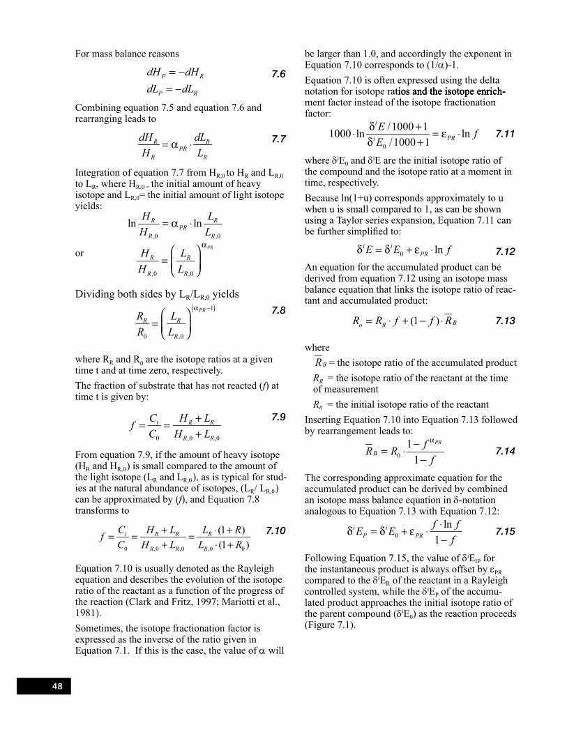
48

For mass balance reasons

P R

P R

dH dHdL dL

= −= −

7.6

Combining equation 7.5 and equation 7.6 and rearranging leads to

R R

PRR R

dH dLH L

= α ⋅ 7.7

Integration of equation 7.7 from HR,0 to HR and LR,0 to LR, where HR,0 = the initial amount of heavy isotope and LR,0= the initial amount of light isotope yields:

,0 ,0

ln lnR RPR

R R

H LH L

= α ⋅

or

,0 ,0

PR

R R

R R

H LH L

α

=

Dividing both sides by LR/LR,0 yields

( )1

0 ,0

PR

R R

R

R LR L

−α

=

7.8

where RR and R0 are the isotope ratios at a given time t and at time zero, respectively. The fraction of substrate that has not reacted (f) at time t is given by:

0 ,0 ,0

t R R

R R

C H LfC H L

+= =+

7.9

From equation 7.9, if the amount of heavy isotope (HR and HR,0 ) is small compared to the amount of the light isotope (LR and LR,0 ), as is typical for stud-ies at the natural abundance of isotopes, (LR/ LR,0 ) can be approximated by (f), and Equation 7.8 transforms to

0 ,0 ,0 ,0 0

(1 )(1 )

t R R R

R R R

C H L L RfC H L L R

+ ⋅ += = =+ ⋅ +

7.10

Equation 7.10 is usually denoted as the Rayleigh equation and describes the evolution of the isotope ratio of the reactant as a function of the progress of the reaction (Clark and Fritz, 1997; Mariotti et al., 1981). Sometimes, the isotope fractionation factor is expressed as the inverse of the ratio given in Equation 7.1. If this is the case, the value of a will

be larger than 1.0, and accordingly the exponent in Equation 7.10 corresponds to (1/a)-1.Equation 7.10 is often expressed using the delta notation for isotope ratios and the isotope enrich-tios and the isotope enrich-ios and the isotope enrich-ment factor instead of the isotope fractionation factor:

0

/1000 11000 ln ln/1000 1

i

PRi

E fE

δ +⋅ = ε ⋅δ +

7.11

where δiE0 and δiE are the initial isotope ratio of the compound and the isotope ratio at a moment in time, respectively. Because ln(1+u) corresponds approximately to u when u is small compared to 1, as can be shown using a Taylor series expansion, Equation 7.11 can be further simplified to:

0 lni iPRE E fδ = δ + ε ⋅ 7.12

An equation for the accumulated product can be derived from equation 7.12 using an isotope mass balance equation that links the isotope ratio of reac-tant and accumulated product:

(1 ) Bo RR R f f R= ⋅ + − ⋅ 7.13

whereBR = the isotope ratio of the accumulated product

RR = the isotope ratio of the reactant at the time of measurementR0 = the initial isotope ratio of the reactant

Inserting Equation 7.10 into Equation 7.13 followed by rearrangement leads to:

0

11

PR

BfR R

f

α−= ⋅−

7.14

The corresponding approximate equation for the accumulated product can be derived by combined an isotope mass balance equation in δ-notation analogous to Equation 7.13 with Equation 7.12:

0ln

1i i

P PRf fE E

f⋅δ = δ + ε ⋅−

7.15

Following Equation 7.15, the value of δiEIP for the instantaneous product is always offset by ePR compared to the δiER of the reactant in a Rayleigh controlled system, while the δiEP of the accumu-lated product approaches the initial isotope ratio of the parent compound (δiE0) as the reaction proceeds (Figure 7.1).

49

Figure 7.1. Simulated evolution of carbon isotope ratios of reactant (TCE) and degrada-tion product (cis-DCE) according to the Rayleigh equation. The isotope evolution of the product that is formed at a certain moment in time (instan-taneous product) as well as the aver-age isotope ratio of the accumulation product is shown. The average cis-DCE deviates from the instantaneous product to more depleted values as it is a mixture of product that accumulates from the start of the reaction. As the instantaneous product becomes heavi-er, the accumulated product becomes heavier. The enrichment factor e stays constant over time. An isotope enrich-ment factor of -8.5‰ was assumed in the simulation.

7.3. Quantification of Isotope Fractionation in Laboratory Studies

Laboratory data should be evaluated using the full Rayleigh equation (Equation 7.10) unless the exper-iments were carried out with labelled compounds. In this case, it is necessary to use an equation derived from Equation 7.8 without simplifications. When the uncertainty of the measurement is in the same range as the uncertainty of the isotope ratio of the reference gas, the following linearized form of Equation 7.10 is recommended to quantify aPR:

( )0 0

/1000 1ln ln 1 ln/1000 1

i

PRi

R E fR E

δ += = α − ⋅δ +

7.16

The linear regression should be carried out with-out forcing the regression line through the origin. Laboratory experiments are often carried out in replicates, which raises the question of how the data should be combined to obtain a representa-tive fractionation factor. The non-weighted average

fractionation factor should only be used if the replicates consist of a similar number of observa-tions spread over a similar range in f. Otherwise, Scott et al. (2004) propose a method based on linear regression with dummy variable and a method based on a Pitman estimator.

7.4. Equations to Evaluate Field Isotope Data

Under certain conditions (see Section 3), the degree of biodegradation or the first order rate constant for biodegradation can be quantified for the zone between the source and a monitoring point, or between two monitoring points along a flow path. By rearrangement of equation 7.16, the following equation is obtained to quantify the fraction remain-ing (f):

1 10001

0 0

10001000

PR PRi

i

R EfR E

−α ε δ += = δ +

7.17

whereδiE = the isotope ratio at the downgradient monitoring point, and δiE0 = the isotope ratio at the source or upgradient monitoring point.

The amount of biodegradation or abiotic trans-formation (in percent of the material originally present) is given by:

(1 ) 100B f= − ⋅ 7.18

The change in the isotope ratio from the source area to a monitoring well or from well to well can be used for two purposes. The CSIA data can be used to test the hypothesis that the concentration decrease is predominantly due to biodegradation or abiotic transformation, and the data can be used to extrapolate the removal that would be expected further along the flow path. The expected concen-tration at a down gradient monitoring point can be calculated using:

exp oC C f= ⋅ 7.19

where Cexp = the expected concentration at the down gradient monitoring pointC0 = the concentration at the source or the up gradient monitoring point along a flow path.

50

If the reductions in concentrations are due to a particular process that has a characteristic value for ePR , then the value of (f) as obtained from Equation 7.17, should substitute into Equation 7.19 to predict a value for Cexp that is in good agreement with the measured concentration in the down gradi-ent monitoring well. If the values are not in good agreement, then it is possible that other processes such as dilution in the well or dispersion along the flow path has a stronger influence on the measured concentration. If is also possible that there is an error in the conceptual model, that some other pro-cess is responsible for destruction of the compound, and the assumed value of ePR is in error. The CSIA data can also be used to extrapolate con-taminant degradation further down the flow path. The first order rate constant for contaminant remov-al can be estimated by combining Equation 7.10 with the equation describing first-order degradation of a substance:

0

exp( )tCf TC

= = −λ ⋅ 7.20

where:T = the average travel time of the compounds of interest between source and monitoring point or between two monitoring points along a flow line. For retarded compounds, the travel time is given by T=RT∙Tw where RT is the retardation factor and Tw is the average travel time of water, lt = the first order rate constant for reduction in concentration due to biodegradation or abiotic transformation.

Solving Equation 7.20 for lt, and then substituting Equation 7.17 for f, produces Equation 7.21.

0 0

1 1000 1000ln ln1 1000

i

iPR PR

t

R ER E

T T

δ +⋅ ⋅α − ε δ +

λ = − = −

7.21

The calculated rate constant represents the rate of removal from biodegradation or abiotic transforma-tion. The rate of removal is distinct from the bulk attenuation rate k that is calculated by plotting the natural logarithm of the concentrations against the time of travel along the flow path (Newell et al., 2002). The bulk attenuation rate also includes the effect of dilution through dispersion on the concen-tration in addition to the effect of removal.

Equation 7.20 can be solved for the travel time required along the flow path (Trequired) to attain any desired concentration (Crequired) at the field-scale rate of removal lt.

0

ln /requiredrequired t

CT

C

= − λ 7.22

Multiplication of (Trequired) by the contaminant velocity (Vseepage) yields an equation for the distance along the flow path from the source or the up gradi-ent monitoring well that is required to reduce the contaminant concentration to the desired concentra-tion (Lrequired).

0

ln *( ) /requiredrequired seepage t

CL V

C

= − λ 7.23

where Vseepage = the actual seepage velocity of the contaminant in ground water along the flow path.

The seepage velocity is usually estimated by divid-ing the Darcy velocity by the effective porosity, and then dividing by the retardation factor for the contaminant. If the value of Crequired is a Maximum Contaminant Level (MCL), a clean up goal, or other regulatory standard, a value for Lrequired can be used to estimate a perimeter beyond which the concentrations of a contaminant should no longer be of regulatory con-cern. The value of Lrequired can be calculated without knowledge of the ground water flow velocity. The calculation of Lrequired is conservative because it does not include reductions in concentrations caused by dilution or dispersion.

51

8.0Stable Isotope Enrichment Factors

This section summarizes the isotope enrichment factors that are available in the literature at the time this section was written. However, the literature on isotope fractionation is growing rapidly, and this section is only offered as a point of departure. The reader should perform a literature search to update the information needed for a particular application.

Table 8.1. Isotope enrichment factors (e) for aerobic and anaerobic biodegradation of selected ground water pollutants. Intrinsic enrichment factors (ei ) for carbon isotope fractionation have been calculated following Morasch et al. ( 2004), where ei = e *n. Values of ei are provided in the third column to illustrate the isotope

effect at the atom where the reaction takes place.

Compound13C/12C

fractionationIntrinsic

13C/12C fractionation

Fraction-ation of other

elementsConditions Bacteria Reference

BTEX Compounds

Benzene e = -1.46 ei = -8.82H/1H:e = -12 Oxic

Acinetobacter sp. (Hunkeler et al., 2001b)

Benzene e = -3.53 ei = -21.22H/1H:e = -11. Oxic Burkholderia sp. (Hunkeler et

al., 2001b)

Benzene e = -2.4e = -2.0

ei = -14.4ei = -12

2H/1H:e = -29e = -35

Nitrate-reducing Enrichment culture (Mancini et

al., 2003)

Benzene e = -3.6 ei = -21.62H/1H:e = -79

Sulfate-reducing Enrichment culture (Mancini et

al., 2003)

Benzene e = -1.9e = -2.1

ei = -11.4ei = -12.6

2H/1H:e = -60 Methanogenic Enrichment culture

(Mancini et al., 2002)

(Mancini et al., 2003)

Ethylbenzene e = -2.2 ei = -17.6 Nitrate-reducing Strain EBN1 (Meckenstock

et al., 2004)

Ethylbenzene e = -3.7 ei = -30 Sulfate-reducing Enrichment culture (Wilkes et al.,

2000)

Toluene Not significant Oxic Microcosms(Sherwood Lollar et al.,

1999)

Toluene e = -3.3 ei = -23.1 Oxic Pseudomonas putida strain mt-2

(Morasch et al., 2002)

52

Compound13C/12C

fractionationIntrinsic

13C/12C fractionation

Fraction-ation of other

elementsConditions Bacteria Reference

Toluene

e = -1.7 (high iron)

e = -2.5 (low iron)

ei = -11.9

ei = -17.5

2H/1H:e = -77

(high iron)e = -159

(low iron)

Oxic Pseudomonas putida strain mt-2

(Mancini et al., 2006)

Toluene e = -1.1 ei = -7.7 Oxic Ralstonia pickettii strain PKO1

(Morasch et al., 2002)

Toluene e = -0.4 ei = -2.8 Oxic Pseudomonas putida strain F1

(Morasch et al., 2002)

Toluene e = -1.7 ei = -11.9 Nitrate-reducing Thauera aromatica (Meckenstock

et al., 1999)

Toluene e = -1.8 ei = -12.6 Fe(III)- reducing

Geobacter metallireducens

(Meckenstock et al., 1999)

Toluene e = -0.8 ei = -5.6 Sulfate-reducing Enrichment culture (Ahad et al.,

2000)

Toluene e = -1.5 ei = -10.5 Sulfate-reducing

Column experiment

(Meckenstock et al., 1999)

Toluene e = -2.2 ei = -15.4 Sulfate-reducing

Desulfobacterium cetonicum

(Morasch et al., 2001)

Toluene e = -1.7 ei = -11.9 Sulfate-reducing Strain TRM1 (Meckenstock

et al., 1999)

Toluene2H/1H:

e = -728Sulfate-reducing strain TRM1 (Morasch et

al., 2001)

Toluene2H/1H:

e = -198Sulfate-reducing

Desulfobacterium cetonicum

(Morasch,et al., 2001)

Toluene e = -0.5 ei = -3.5 Methanogenic Enrichment culture (Ahad et al., 2000)

Toluene2H/1H:e = -12e = -65

Methanogenic Consortium (Ward et al., 2000)

m-Xylene e = -1.7 ei = -13.6 Oxic Pseudomonas putida strain mt-2

(Morasch et al., 2002)

m-Xylene e = -1.8 ei = -14.4 Sulfate-reducing Strain OX39 (Morasch et

al., 2004)

p-Xylene e = -2.3 ei = -18.4 Oxic Pseudomonas putida strain mt-2

(Morasch et al., 2002)

o-Xylene e = -1.5 ei = -12 Sulfate-reducing Strain OX39 (Morasch et

al., 2004)

53

Compound13C/12C

fractionationIntrinsic

13C/12C fractionation

Fraction-ation of other

elementsConditions Bacteria Reference

o-Xylene e = -1.1 ei = -8.8 Sulfate-reducing

Column experiment

(Richnow et al., 2003)

o-Xylene e = -3.2 ei = -25.6 Sulfate-reducing Enrichment culture (Wilkes et al.,

2000)

m-Cresol e = -3.9 ei = -27.3 Sulfate-reducing

Desulfobacterium cetonicum

(Morasch,et al., 2004)

p-Cresol e = -1.6 ei = -11.2 Sulfate-reducing

Desulfobacterium cetonicum

(Morasch et al., 2004)

Polyaromatic Hydrocarbons

Naphthalene e = -0.1 ei = -1.1 OxicPseudomonas putida strain NCIB9816

(Morasch et al., 2002)

Naphthalene e = -1.1 ei = -11 Sulfate-reducing

Enrichment culture N47

(Griebler et al., 2004b)

2-Methyl-naphthalene e = -0.9 ei = -9.9 Sulfate-

reducingEnrichment culture

N47(Griebler et al., 2004b)

2-Methyl-phenanthrene

No enrichment Oxic Sphingomonas sp.

strain 2MPII(Mazeas and Budzinski,

2002)

Fluoranthene No enrichment Oxic Sphingomonas

paucimobilis(Hammer et al., 1998)

Chlorinated Hydrocarbons

PCE37Cl/35Cle = -10

Anoxic, dehalogenating

Strain T, consortium N, consortium F

(Numata et al., 2002)

PCE e = -5.2 ei = -10.4 Anoxic, dehalogenating

Consortium (butyric acid)

(Slater et al., 2001)

PCEEnrichment estimated

2‰

Anoxic, dehalogenating

Microcosm experiment

(Hunkeler et al., 1999)

PCE e = -5.2 to -8.8

ei = -10.4 to -17.6

Anoxic, dehalogenating

Desulfitobacterium sp. PCE-S

(Nijenhuis et al., 2005)

PCE e = -0.42 to -1.7

ei = -0.84 to -3.4

Anoxic, dehalogenating

Sulfurospirillum multivorans

(Nijenhuis et al., 2005)

PCE e = -0.46 to -3.2

ei = -0.92 to -6.4

Anoxic, dehalogenating

Sulfurospirillum halorespirans

(Cichocka et al., 2007)

TCE e = -18.2 ei = -36.4 Oxic Burkholderia cepacia strain G4

(Bill et al., 2001)

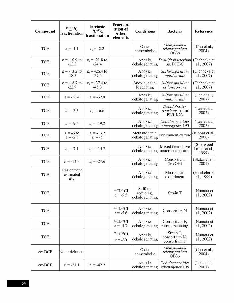
54

Compound13C/12C

fractionationIntrinsic

13C/12C fractionation

Fraction-ation of other

elementsConditions Bacteria Reference

TCE e = -1.1 ei = -2.2 Oxic, cometabolic

Methylosinus trichosporium

OB3b(Chu et al.,

2004)

TCE e = -10.9 to -12.2

ei = -21.8 to -24.4

Anoxic, dehalogenating

Desulfitobacterium sp. PCE-S

(Cichocka et al., 2007)

TCE e = -13.2 to -18.7

ei = -26.4 to -37.4

Anoxic, dehalogenating

Sulfurospirillum multivorans

(Cichocka et al., 2007)

TCE e = -18.7 to -22.9

ei = -37.4 to -45.8

Anoxic, deha-logenating

Sulfurospirillum halorespirans

(Cichocka et al., 2007)

TCE e = -16.4 ei = -32.8 Anoxic, dehalogenating

Sulfurospirillum multivorans

(Lee et al., 2007)

TCE e = -3.3 ei = -6.6 Anoxic, dehalogenating

Dehalobacter restrictus strain

PER-K23(Lee et al.,

2007)

TCE e = -9.6 ei = -19.2 Anoxic, dehalogenating

Dehalococcoides ethenogenes 195

(Lee et al., 2007)

TCE e = -6.6;e = -2.5

ei = -13.2ei = -5

Methanogenic, dehalogenating Enrichment culture (Bloom et al.,

2000)

TCE e = -7.1 ei = -14.2 Anoxic, dehalogenating

Mixed facultative anaerobic culture

(Sherwood Lollar et al.,

1999)

TCE e = -13.8 ei = -27.6 Anoxic, dehalogenating

Consortium (MeOH)

(Slater et al., 2001)

TCEEnrichment estimated

4‰

Anoxic, dehalogenating

Microcosm experiment

(Hunkeler et al., 1999)

TCE37Cl/35Cle = -5.5

Sulfate-reducing,

dehalogenatingStrain T (Numata et

al., 2002)

TCE37Cl/35Cle = -5.6

Anoxic, dehalogenating Consortium N (Numata et

al., 2002)

TCE37Cl/35Cle = -5.7

Anoxic, dehalogenating

Consortium F, nitrate reducing

(Numata et al., 2002)

TCE37Cl/35Cl e = -30

Anoxic, dehalogenating

Strain T, consortium N, consortium F

(Numata et al., 2002)

cis-DCE No enrichment Oxic, cometabolic

Methylosinus trichosporium

OB3b(Chu et al.,

2004)

cis-DCE e = -21.1 ei = -42.2 Anoxic, dehalogenating

Dehalococcoides ethenogenes 195

(Lee et al., 2007)

55

Compound13C/12C

fractionationIntrinsic

13C/12C fractionation

Fraction-ation of other

elementsConditions Bacteria Reference

cis-DCE e = -16.9 ei = -33.8 Anoxic, dehalogenating

Dehalococcoides sp. Strain BAV1

(Lee et al., 2007)

cis-DCE e = -14.1e = -16.1

ei = -28.2ei = -32.2

Methanogenic, dehalogenating Enrichment culture (Bloom et al.,

2000)

cis-DCE e = -19.9 ei = -39.8 Anoxic, dehalogenating Microcosms (Hunkeler et

al., 2002)

cis-DCE e = -20.4 ei = -40.8 Anoxic, dehalogenating

Consortium (MeOH)

(Slater et al., 2001)

cis-DCEEnrichment estimated

12‰Anoxic,

dehalogenatingMicrocosm experiment

(Hunkeler et al., 1999)

trans-DCE e = -3.5 ei = -7 Oxic, cometabolic

Methylomonas methanica

(Brungard et al., 2003)

trans-DCE e = -6.7 ei = -13.4 Oxic, cometabolic

Methylosinus trichosporium

OB3b(Brungard et

al., 2003)

trans-DCE e = -21.4 ei = -42.8 Anoxic, dehalogenating

Dehalococcoides sp. Strain BAV1

(Lee et al., 2007)

trans-DCE e = -30.3 ei = -60.6 Anoxic, dehalogenating Microcosms (Hunkeler et

al., 2002)

1,1-DCE e = -7.3 ei = -14.6 Anoxic, dehalogenating Microcosms (Hunkeler et

al., 2002)

1,1-DCE e = -5.8 ei = -11.2 Anoxic, dehalogenating

Dehalococcoides ethenogenes 195

(Lee et al., 2007)

1,1-DCE e = -8.4 ei = -16.8 Anoxic, dehalogenating

Dehalococcoides sp. Strain BAV1

(Lee et al., 2007)

VC e = -5.7 ei = -11.4 Oxic, metabolic

Mycobacterium aurum L1

(Chu et al., 2004)

VC e = -3.2 ei = -6.4 Oxic, cometabolic

Methylosinus trichosporium

OB3b(Chu et al.,

2004)

VC e = -4.8 ei = -9.6 Oxic, cometabolic

Mycobacterium vaccae JOB5

(Chu et al., 2004)

VC e = -4.5 ei = -9.0 Oxic, cometabolic

Enrichment culture Travis

(Chu et al., 2004)

VC e = -5.5 ei = -11 Oxic, cometabolic

Enrichment culture Alameda

(Chu et al., 2004)

VC e = -8.2 ei = -16.4 Oxic Mycobacterium sp. JS60

(Chartrand et al., 2005)

VC e = -7.1 ei = -14.2 Oxic Mycobacterium sp. JS61

(Chartrand et al., 2005)

VC e = -7.1 ei = -14.2 Oxic Mycobacterium sp. JS617

(Chartrand et al., 2005)

56

Compound13C/12C

fractionationIntrinsic

13C/12C fractionation

Fraction-ation of other

elementsConditions Bacteria Reference

VC e = -7.6 ei = -15.2 Oxic Nocardioides sp.JS614

(Chartrand et al., 2005)

VC e = -24.0 ei = -48 Anoxic, dehalogenating

Dehalococcoides sp. Strain BAV1

(Lee et al., 2007)

VC e = -21.5 ei = -43 Methanogenic, dehalogenating Enrichment culture (Bloom et al.,

2000)

VC e = -22.4 ei = -44.8 Anoxic, dehalogenating

Consortium (MeOH)

(Slater et al., 2001)

VC e = -31.1 ei = -62.2 Anoxic, dehalogenating Microcosms (Hunkeler et

al., 2002)

VC e estimated-26

Anoxic, dehalogenating

Microcosm experiment

(Hunkeler et al., 1999)

Dichloro-methane

37Cl/35Cle = -3.8 Oxic Biodegradation (Holt et al.,

1997)

Dichloro-methane

e = -41 to -66

ei = -41 to -66 Oxic

Various methylotrophic

bacteria(Nikolausz et

al., 2006)

Dichloro-methane

e = -46 to -61

ei = -45 to -61 Denitrifying

Various methylotrophic

bacteria(Nikolausz et

al., 2006)

1,2-Dichloro-ethane

e = -32e = -27

ei = -64ei = -54 Oxic Xanthobacter

autotrophicus(Hunkeler

and Aravena, 2000a)

1,2-Dichloro-ethane e = -32.1 ei = -64.2 Anoxic,

dehalogenating Microcosms (Hunkeler et al., 2002)

1,2-Dichloro-ethane e = -32.3 ei = -64.6 Oxic Xanthobacter

autotrophicus GJ10(Hirschorn et

al., 2004)1,2-Dichloro-

ethane e = -32.1 ei = -64.2 Oxic Ancylobacter aquaticus AD20

(Hirschorn et al., 2004)

1,2-Dichloro-ethane e = -3.0 ei = -6.0 Oxic Pseudomonas sp.

StrainDCA1(Hirschorn et

al., 2004)1,1,2-Trichloro-

ethane e = -2.0 ei = -4 Anoxic, dehalogenating Microcosms (Hunkeler et

al., 2002)

Chlorobenzene e = -0.4 e = -2.4 Oxic Ralstonia sp. (Kaschl et al., 2005)

Chlorobenzene e = -0.3 e = -1.8 Oxic R. erythropolis (Kaschl et al., 2005)

Chlorobenzene e = -0.2 e = -1.2 Oxic P. veronii (Kaschl et al., 2005)

Chlorobenzene e = -0.1 e = -0.6 Oxic A. facilis (Kaschl et al., 2005)

1,2,4-Trichloro-benzene Not significant Oxic Pseudomonas sp.

strain P51(Griebler et al., 2004a)

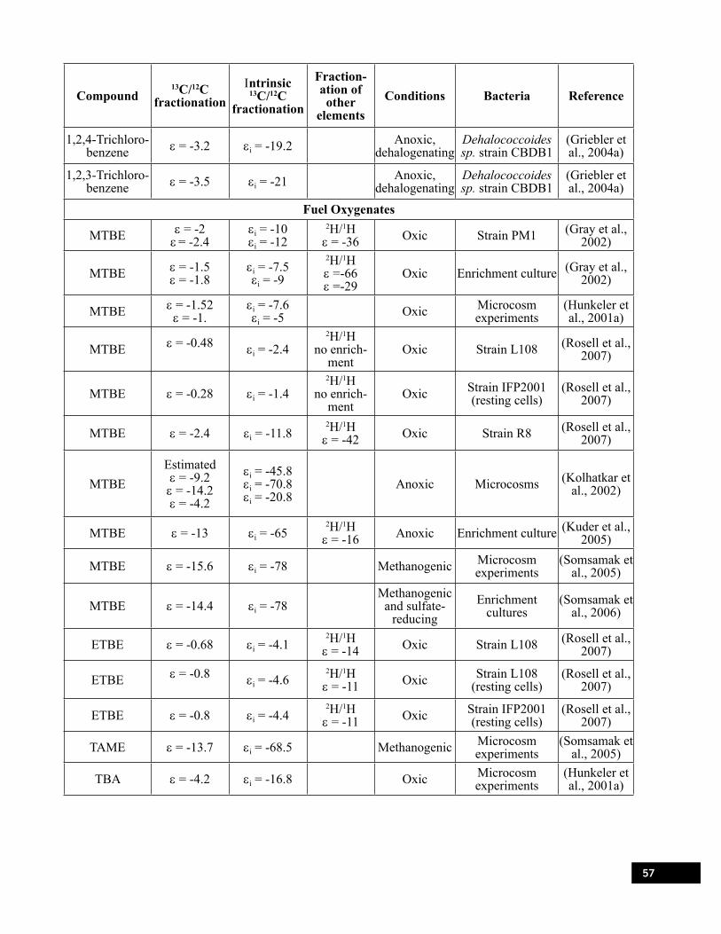
57

Compound13C/12C

fractionationIntrinsic

13C/12C fractionation

Fraction-ation of other

elementsConditions Bacteria Reference

1,2,4-Trichloro-benzene e = -3.2 ei = -19.2 Anoxic,

dehalogenatingDehalococcoides sp. strain CBDB1

(Griebler et al., 2004a)

1,2,3-Trichloro-benzene e = -3.5 ei = -21 Anoxic,

dehalogenatingDehalococcoides sp. strain CBDB1

(Griebler et al., 2004a)

Fuel Oxygenates

MTBE e = -2e = -2.4

ei = -10ei = -12

2H/1He = -36 Oxic Strain PM1 (Gray et al.,

2002)

MTBE e = -1.5e = -1.8

ei = -7.5ei = -9

2H/1He =-66e =-29

Oxic Enrichment culture (Gray et al., 2002)

MTBE e = -1.52e = -1.

ei = -7.6ei = -5 Oxic Microcosm

experiments(Hunkeler et al., 2001a)

MTBE e = -0.48 ei = -2.42H/1H

no enrich-ment

Oxic Strain L108 (Rosell et al., 2007)

MTBE e = -0.28 ei = -1.42H/1H

no enrich-ment

Oxic Strain IFP2001 (resting cells)

(Rosell et al., 2007)

MTBE e = -2.4 ei = -11.82H/1H

e = -42 Oxic Strain R8 (Rosell et al., 2007)

MTBEEstimated e = -9.2e = -14.2e = -4.2

ei = -45.8ei = -70.8ei = -20.8

Anoxic Microcosms (Kolhatkar et al., 2002)

MTBE e = -13 ei = -652H/1H

e = -16 Anoxic Enrichment culture (Kuder et al., 2005)

MTBE e = -15.6 ei = -78 Methanogenic Microcosm experiments

(Somsamak et al., 2005)

MTBE e = -14.4 ei = -78Methanogenic

and sulfate-reducing

Enrichment cultures

(Somsamak et al., 2006)

ETBE e = -0.68 ei = -4.12H/1H

e = -14 Oxic Strain L108 (Rosell et al., 2007)

ETBE e = -0.8 ei = -4.62H/1He = -11 Oxic Strain L108

(resting cells)(Rosell et al.,

2007)

ETBE e = -0.8 ei = -4.42H/1He = -11 Oxic Strain IFP2001

(resting cells)(Rosell et al.,

2007)

TAME e = -13.7 ei = -68.5 Methanogenic Microcosm experiments

(Somsamak et al., 2005)

TBA e = -4.2 ei = -16.8 Oxic Microcosm experiments

(Hunkeler et al., 2001a)

58

9.0Recommendations for the Application of CSIA

Compound Specific Isotope Analysis (CSIA) provides another dimension of information on pollutants in the environment to supplement knowledge of their chemical identity and their concentration. CSIA has matured into a technique that can be used on a routine basis, in particular for carbon isotope analysis, for a wide range of organic contaminants relevant to hydrogeology and envi-ronmental geochemistry. Modern instrumentation can provide valid determinations of isotope ratios at low concentrations of contaminants that are near their regulatory standards or clean-up goals. Application of CSIA at a contaminated site should start with a clear idea of the information that is sought from stable isotope analysis. Basically, there are three distinct goals: (i) source character-ization or differentiation; (ii) qualitative proof of biodegradation or abiotic transformation; or, (iii) quantification of biodegradation or abiotic trans-formation processes. Advantages and limitations of the use of CSIA for these purposes have been discussed in detail throughout this guideline. If the specific interest is quantification of degradation, the first step is to consult the literature (summarized in Table 8.1) to determine whether an appropriate isotopic enrichment factor is available. Using the enrichment factor, the second step is to estimate whether the observed changes in concentration of the contaminant at the field site are sufficient to produce a measurable change in the isotope ratio. If these two prerequisites are met there is a good chance that it will be possible to put a conservative boundary on the extent of biodegradation or abiotic transformation at the field site. On a per sample basis, the cost of an individual isotope analysis is substantially higher than the cost of a VOC analysis to identify the chemical, and determine its concentration. This is due to the price of the equipment required to perform CSIA, the costs of consumables, the level of training and ex-perience required for the analytical chemist, and the number of standards and sample duplicates that are needed to ensure reliable data as discussed in sec-tion 2.4. However, a simple comparison of direct costs for analyses is not very meaningful. Instead, consider the total cost of a site investigation. If the

additional information from CSIA leads to a robust conceptual model for a site, it can lead to savings in conventional monitoring. If there is greater faith in the site conceptual model, adequate monitoring can be attained with fewer rounds of sampling and analysis, and fewer monitoring wells. Furthermore, CSIA can guide decisions on selec-tion and implementation of remediation strategies, and can be used to monitor the performance of remedial technology in an early stage of imple-mentation. Thus, the huge waste in resources that are associated with the selection of an unsuitable remediation strategy might be avoided. Compound specific isotope analysis can be applied on a routine basis when precautions are taken to ensure high quality data and the appropriate in-terpretation of the data. However, CSIA cannot replace a proper hydrological and geochemical characterization or measurements of contaminant concentrations. Multiple lines of evidence will continue to be necessary to come to a meaningful assessment of the risks associate with the contami-nants and the selection of an appropriate remedy. It is our hope that this Guide will be a useful in-troduction for beginners in environmental isotope analysis. We expect that CSIA will have a grow-ing role in investigations at hazardous waste sites. The growth in the application of CSIA is driven by continued improvements in analytical methods, by more widespread availability of the instruments used in CSIA, by an increasing number of publica-tions showing the broad applicability of CSIA to a variety of contaminants, and by an increasing appreciation for the unique information provided by CSIA. We have only “scratched the surface” of the potential of CSIA to provide a better understanding of the source, distribution, and behavior of organic compounds at contaminated field sites.

59

10.0 References

Abe, Y. and D. Hunkeler. Does the Rayleigh equa-tion apply to evaluate field isotope data in contaminant hydrogeology? Environmental Science and Technology 40: 1588-1596 (2006).

Aguilera, R., C. K. Hatton and D. H. Catlin. Detection of epitestosterone doping by isotope ratio mass spectrometry. Clinical Chemistry 48: 629-636 (2002).

Ahad, J. M. E., B. Sherwood Lollar, E. A. Edwards, G. F. Slater and B. E. Sleep. Carbon isotope fractionation during anaerobic biodegradation of toluene: Implications for intrinsic bioreme-diation. Environmental Science Technology 34: 892-896 (2000).

Arp, H. P. H. and T. C. Schmidt. Air-water trans-fer of MTBE, its degradation products, and alternative fuel oxygenates: The role of tem-perature. Environmental Science Technology 38: 5405-5412 (2004).

Asche, F., O. Gjølberg and T. Völker. Price rela-tionships in the petroleum market: an analysis of crude oil and refined product prices. Energy Economics 25 (3): 289-301 (2003).

Barcelona, M. J., J. P. Gibb, J. A. Helfrich and E. E. Garske. Practical Guide for Ground-Water Sampling, EPA/600/2-85/104. U. S. Environmental Protection Agency, 1985.

Beneteau, K. M., R. Aravena and S. K. Frape. Isotopic characterization of chlorinated sol-vents-laboratory and field results. Organic Geochemistry 30: 739-753 (1999).

Béranger, S., B. E. Sleep, B. Sherwood Lollar and F. P. Monteagudo. Transport, biodegrada-tion and isotopic fractionation of chlorinated ethenes: Modeling and parameter estima-tion methods. Advances in Water Research 28 (1): 87-98 (2005).

Berg, M., J. Bolotin and T. B. Hofstetter. Compound-specific nitrogen and carbon iso-tope analysis of nitroaromatic compounds in aqueous samples using solid-phase micro-extraction coupled to GC/IRMS. Analytical Chemistry 79: 2386-2393 (2007).

Bigeleisen, J. and M. Wolfsburg. Theoretical and experimental aspects of isotope effects in chemical kinetics. Advances in Chemical Physics 1: 15-76 (1959).

Bill, M., C. Schüth, J. A. C. Barth and R. M. Kalin. Carbon isotope fractionation during abiotic reductive dehalogenation of trichloroethene (TCE). Chemosphere 44: 1281-1286 (2001).

Blessing, M., M. A. Jochmann and T. C. Schmidt. Pitfalls in compound-specific isotope analysis of environmental samples. Analytical and Bioanalytical Chemistry 390: 591-603 (2008).

Bloom, Y., R. Aravena, D. Hunkeler, E. Edwards and S. K. Frape. Carbon isotope fractionation during microbial dechlorination of trichloroeth-ene, cis-1, 2-dichloroethene, and vinyl chloride: Implications for assessment of natural attenu-ation. Environmental and Science Technology 34: 2768-2772 (2000).

Bouchard, D., D. Hunkeler, P. Gaganis, R. Aravena, P. Höhener, M. M. Broholm and P. Kjeldsen. Carbon isotope fractionation during diffusion and biodegradation of petroleum hydrocar-bons in the unsaturated zone: field experiment at Værløse Airbase, Denmark, and model-ing. Environmental Science and Technology, 42 (2): 596-601 (2008).

Boyd, T. J., C. L. Osburn, K. J. Johnson, K. B. Birgl and R. B. Coffin. Compound-specific isotope analysis coupled with multivariate statistics to source-apportion hydrocarbon mix-tures. Environmental Science and Technology 40 (6): 1916-1924 (2006).

Bradley, P. M. and F. H. Chapelle. Rapid toluene mineralization by aquifer microorganisms at Adak, Alaska: implications for intrin-sic bioremediation in cold environments. Environmental Science and Technology 29 (11): 2778-2781 (1995).

Bradley, P. M. and F. H. Chapelle. Kinetics of DCE and VC mineralization under methanogenic and Fe(III)-reducing conditions. Environmental Science and Technology 31: 2692-2696 (1997).

Bradley, P. M., S. Richmond and F. H. Chapelle. Chloroethene biodegradation in sediments at 4oC. Applied Environmental Microbiology 71 (10): 6414-6417 (2005).

Brungard, K. L., J. Munakata-Marr, C. A. Johnson and K. W. Mandernack. Stable carbon isotope fractionation of trans-1,2-dichloro-ethylene during co-metabolic degradation by

60

methanotrophic bacteria. Chemical Geology 195: 59-67 (2003).

Butler, E. C. and K. F. Hayes. Kinetics of the transformation of trichlorethylene and tetra-chlorethylene by iron sulfide. Environmental Science and Technology 33: 2021-2027 (1999).

Cervini-Silva, J., R. A. Larson, J. Wu and J. W. Stucki. Transformation of chlorinated aliphatic compounds by ferruginous smec-tite. Environmental Science and Technology 35: 805-808 (2001).

Chartrand, M. M. G., A. Waller, T. E. Mattes, M. Elsner, G. Lacrampe-Couloume, J. M. Gossett, E. A. Edwards and B. Sherwood Lollar. Carbon isotopic fractionation during aerobic vinyl chloride degradation. Environmental Science and Technology 39: 1064-1070 (2005).

Chu, K.-H., S. Mahendra, D. L. Song, M. E. Conrad and L. A. Cohen. Stable carbon iso-tope fractionation during aerobic degradation of chlorinated ethenes. Environmental Science and Technology 38: 3126-3130 (2004).

Cichocka, D., M. Siegert, G. Imfeld, J. Andert, K. Beck, G. Diekert, H. H. Richnow and I. Nijenhuis. Factors controlling the carbon isotope fractionation of tetra- and trichloro-ethene during reductive dechlorination by Sulfurospirillum ssp. and Desulfitobacterium sp. strain PCE-S. FEMS Microbiology Ecology 62: 98-107 (2007).

Clark, I. D., and P. Fritz. Environmental Isotopes in Hydrogeology. CRC Press, Boca Raton, FL, 1997, 328 pages.

Coplen, T. B., W. A. Brand, M. Gehre, M. Gröning, H. A. J. Meijer, B. Toman and R. M. Verkouteren. New guidelines for δ13C measure-ments. Analytical Chemistry 78: 2439-2441 (2006).

Dayan, H., T. Abrajano, N. C. Sturchio and L. Winsor. Carbon isotopic fractionation during reductive dehalogenation of chlorinated eth-enes by metallic iron. Organic Geochemistry 30: 755-763 (1999).

Dempster, H. S., B. Sherwood Lollar and S. Feenstra. Tracing organic contaminants in groundwater: A new methodology us-ing compound-specific isotopic analysis. Environmental Science and Technology 31: 3193-3197 (1997).

Dias, R. F. and K. H. Freeman. Carbon isotope analyses of semivolatile organic compounds in aqueous media using solid-phase

microextraction and isotope ratio monitoring GC/MS. Analytical Chemistry 69: 944-950 (1997).

Elsner, M., L. Zwank, D. Hunkeler and R. P. Schwarzenbach. A new concept linking observable stable isotope fractionation to transformation pathways of organic pollut-ants. Environmental Science and Technology 39: 6896-6916 (2005).

Elsner, M., D. M. Cwiertney, A. L. Roberts and B. Sherwood Lollar. 1, 1, 2, 2-Tetrachloroethane reactions with OH-, Cr(II), granular iron and a copper-iron bimetal: Insights from prod-uct formation and associated carbon isotope fractionation. Environmental Science and Technology 41:4111-4117 (2007a).

Elsner, M., J. Mckelvie, G. Lacrampe Couloume and B. Sherwood Lollar. Insight into methyl tert-butyl ether (MTBE) stable isotope frac-tionation from abiotic reference experiments. Environmental Science and Technology 41:5693-5700 (2007b).

Elsner, M., M. Chartrand, N. VanStone, G. Lacrampe Couloume and B. Sherwood Lollar. Identifying abiotic chlorinated ethene deg-radation: Characteristic isotope patterns in reaction products with nanoscale zero valent iron. Environmental Science and Technology 42: 5963-5970 (2008).

Ferrey, M. L., R. T. Wilkin, R. G. Ford and J. T. Wilson. Non-biological removal of cis-dichlor-ethylene and 1,1-dichlorethylene in aquifer sediment containing magnetite. Environmental Science and Technology 38: 1746-1752 (2004).

Fischer, A., J. Bauer, R. U. Meckenstock, W. Stichler, C. Griebler, P. Maloszewski, M. Kästner and H. H. Richnow. A multitracer test proving the reliability of Rayleigh equation-based approach for assessing biodegradation in a BTEX contaminated aquifer. Environmental Science and Technology 40: 4245-4252 (2006).

Fischer, A., K. Theuerkorn, N. Stelzer, M. Gehre, M. Thullner and H. H. Richnow. Applicability of stable isotope fractionation analysis for the characterization of benzene biodegradation in a BTEX-contaminated aquifer. Environmental Science and Technology 41 (10): 3689-3696 (2007).

Fischer, A., I. Herklotz, S. Herrmann, M. Thullner, S. A. B. Weelink, A. J. M. Stams, M. Schlömann, H.-H. Richnow and C. Vogt . Combined carbon and hydrogen isotope frac-tionation investigations for elucidating benzene

61

biodegradation pathways. Environmental Science and Technology 42: 4356-4363 (2008).

Geyer, R., A. D. Peacock, A. Miltner, H. H. Richnow, D. C. White, K. L. Sublette and M. Kästner. In situ assessment of biodegradation potential using biotraps amended with C-13-labeled benzene or toluene. Environmental Science and Technology 39: 4983-4989 (2005).

Gray, J. R., G. Lacrampe-Couloume, D. Gandhi, K. M. Scow, R. D. Wilson, D. M. Mackay and B. Sherwood Lollar. Carbon and hydrogen isotopic fractionation during biodegradation of methyl tert-butyl ether. Environmental Science and Technology 36: 1931-1938 (2002).

Griebler, C., L. Adrian, R. U. Meckenstock and H. H. Richnow. Stable carbon isotope fractionation during aerobic and anaerobic transformation of trichlorobenzene. FEMS Microbiology Ecology 48: 313-321 (2004a).

Griebler, C., M. Safinowski, A. Vieth, H. H. Richnow and R. U. Meckenstock. Combined application of stable carbon isotope analy-sis and specific metabolites determination for assessing in situ degradation of aromatic hydrocarbons in a tar oil-contaminated aqui-fer. Environmental Science and Technology 38: 617-631 (2004b).

Hammer, B. T., C. A. Kelley, R. B. Coffin, L. A. Cifuentes and J. G. Mueller. δ13C values of polycyclic aromatic hydrocarbons col-lected from two creosote-contaminated sites. Chemical Geology 152: 43-58 (1998).

Harrington, R. R., S. R. Poulson, J. I. Drever, P. J. S. Colberg and E. F. Kelly. Carbon isotope systematics of monoaromatic hydrocarbons: vaporization and adsorption experiments. Organic Geochemistry 30: 765-775 (1999).

Hartenbach, A., T. B. Hofstetter, M. Berg, J. Bolotin and R. P. Schwarzenbach. Using nitrogen isotope fractionation to assess abiotic reduction of nitroaromatic compounds. Environmental Science and Technology 40: 7710-7716 (2006).

Hirschorn, S. K., M. J. Dinglasan, M. Elsner, S. A. Mancini, G. Lacrampe-Couloume, E. A. Edwards and B. Sherwood Lollar. Pathway dependent isotopic fractionation during aero-bic biodegradation of 1,2-dichloroethane. Environmental Science and Technology 38: 4775-4781 (2004).

Hirschorn, S. K., A. Grostern, G. Lacrampe-Couloume, E. A. Edwards, L. MacKinnon, C. Repta, D. W. Major and B. Sherwood Lollar. Quantification of biotransformation of

chlorinated hydrocarbons in a biostimulation study: Added value via stable carbon isotope analysis. Journal of Contaminant Hydrology 94: 249-260 (2007).

Hofstetter, T. B., A. Neumann, W. A. Arnold, A. E. Hartenbach, J. Bolotin, C. J. Cramer and R. P. Schwarzenbach. Substituent effects on nitrogen isotope fractionation during abiotic reduction of nitroaromatic compounds. Environmental Science and Technology 42: 1997-2003 (2008).

Hofstetter, T. B., S. M. Bernasconi, R. P. Schwarzenbach, and R. Kretzschmar. New methods for the environmental chemist’s tool-box. Environmental Science and Technology 42: 7727 (2008).

Holmstrand, H., M. Mandalakis, Z. Zencak, O. Gustafsson and P. Andersson. Chlorine isotope fractionation of a semi-volatile organochlorine compound during preparative megabore-column capillary gas chromatography. Journal of Chromatography A 1103: 133-138 (2006).

Holt, B. D., N. C. Sturchio, T. Abrajano and L. J. Heraty. Conversion of chlorinated volatile or-ganic compounds to carbon dioxide and methyl chloride for isotopic analysis of carbon and chlorine. Analytical Chemistry 69: 2727-2733 (1997).

Hunkeler, D. and R. Aravena. Evidence of sub-stantial carbon isotope fractionation among substrate, inorganic carbon, and biomass during aerobic mineralization of 1,2-dichloroethane by Xanthobacter autotrophicus. Applied and Environmental Microbiology 66: 4870-4876 (2000a).

Hunkeler, D., and R. Aravena. Determination of compound-specific carbon isotope ratios of chlorinated methanes, ethanes, and ethenes in aqueous samples. Environmental Science and Technology 34: 2839-2844 (2000b).

Hunkeler, D. R. Aravena and B. J. Butler. Monitoring microbial dechlorination of tet-rachloroethene (PCE) in groundwater using compound-specific stable carbon isotope ratios: Microcosm and field studies. Environmental Science and Technology 33: 2733-2738 (1999).

Hunkeler, D., B. J. Butler, R. Aravena and J. F. Barker. Monitoring biodegradation of methyl tert-butyl ether (MTBE) using compound-spe-cific carbon isotope analysis. Environmental Science and Technology 35: 676-681 (2001a).

Hunkeler, D., N. Anderson, R. Aravena, S. M. Bernasconi and B. J. Butler. Hydrogen and carbon isotope fractionation during aerobic

62

biodegradation of benzene. Environmental Science and Technology 35: 3462-3467 (2001b).

Hunkeler, D. and R. Aravena. Evidence of sub-stantial carbon isotope fractionation among substrate, inorganic carbon, and biomass during aerobic mineralization of 1,2-dichloroeth-ane by Xanthobacter autotrophicus. Applied Environmental Microbiology 66: 4870-4876 (2000c).

Hunkeler, D., R. Aravena and E. Cox. Carbon isotopes as a tool to evaluate the origin and fate of vinyl chloride: laboratory experiments and modeling of isotope evolution. Environmental Science and Technology 36: 3378-3384 (2002).

Hunkeler, D., N. Chollet, X. Pittet, R. Aravena, J. A. Cherry and B. L. Parker. Effect of source variability and transport processes on carbon isotope ratios of TCE and PCE in two sandy aquifers. Journal of Contaminant Hydrology 74: 265-282 (2004).

Hunkeler, D., R. Aravena, K. Berry-Spark and E. Cox. Assessment of degradation pathways in an aquifer with mixed chlorinated hydrocarbon contamination using stable isotope analy-sis. Environmental Science and Technology 39: 5975-5981 (2005).

Jeffers, P. M., L. M. Ward, L. M. Woytowitch and N. L. Wolfe. Homogenous Hydrolysis rate constants for selected chlorinated methanes, ethanes, ethenes, and propanes. Environmental Science and Technology 23: 965-969 (1989).

Jendrzejewski, N., H. G. M. Eggenkamp and M. L. Coleman. Sequential determination of chlo-rine and carbon isotopic composition in single microliter samples of chlorinated solvents. Analytical Chemistry 69: 4259-4266 (1997).

Jendrzejewski, N., H. G. M. Eggenkamp and M. L. Coleman. Characterization of chlorinated hy-drocarbons from chlorine and carbon isotopic compositions: scope of application to environ-mental problems. Applied Geochemistry 16: 1021-1031 (2001).

Jochmann, M. A., M. Blessing, S. B. Haderlein and T. C. Schmidt. A new approach to determine method detection limits for compound specific isotope analysis of volatile organic carbons. Rapid Communications in Mass Spectrometry 20: 3639-3648 (2006).

Kaschl, A., C. Vogt, S. Uhlig, I. Nijenhuis, H. Weiss, M. Kästner and H. H. Richnow. Isotopic fractionation indicates anaero-bic monochlorobenzene biodegradation.

Environmental Toxicology and Chemistry 24: 1315-1324 (2005).

Kirtland, B. C., C. M. Aelion, P. A. Stone and D. Hunkeler. Isotopic and geochemical assess-ment of in situ biodegradation of chlorinated hydrocarbons. Environmental Science and Technology 37: 4205-4212 (2003).

Kolhatkar, R. V., T. Kuder, P. Philp, J. Allen and J. T. Wilson. Use of compound-specific stable carbon isotope analyses to demonstrate anaero-bic biodegradation of MTBE in groundwater at a gasoline release site. Environmental Science and Technology 36: 5139-5146 (2002).

Kopinke, F. D., A. Georgi, M. Voskamp and H. H. Richnow. Carbon isotope fractionation of or-ganic contaminants due to retardation on humic substances: Implications for natural attenuation studies in aquifers. Environmental Science and Technology 39: 6052-6062 (2005).

Kovacs, D. A. and D. H. Kampbell. Improved method for the storage of groundwater samples containing volatile organic analytes. Archives of Environmental Contamination and Toxicology 36: 242-247 (1999).

Kuder, T., R. P. Philp, R. V. Kolhatkar, J. T. Wilson and J. Allen. “Application of stable carbon and hydrogen isotopic techniques for monitoring biodegradation on MTBE in the field.” In Proceedings of the 2002 Petroleum Hydrocarbons and Organic Chemicals in Ground Water: Prevention, Assessment, and Remediation, Conference and Exposition, November 6-8, Atlanta, GA, 2002, 371-381.

Kuder, T., J. T. Wilson, P. Kaiser, R. Kolhatkar, P. Philp and J. Allen. Enrichment of stable car-bon and hydrogen isotopes during anaerobic biodegradation of MTBE: Microcosm and field evidence. Environmental Science and Technology 39: 213-220 (2005).

Lee, W. and B. Batchelor. Abiotic reductive dechlorination of chlorinated ethylenes by iron-bearing soil minerals: 1. pyrite and mag-netite. Environmental Science and Technology 36: 5147-5154 (2002).

Lee, P. K. H., M. E. Conrad and L. Alvarez-Cohen. Stable Carbon Isotope Fractionation of Chloroethenes by Dehalorespiring Isolates. Environmental Science and Technology 41: 4277-4285 (2007).

Liang, X., Y. Dong, T. Kuder, L. R. Krumholz, R. P. Philp and E. C. Butler. Distinguishing abiotic and biotic transformation of tetrachloroethylene and trichloroethylene by stable carbon isotope

63

fractionation. Environmental Science and Technology 41 (20): 7094-7100 (2007).

Mancini, S. A., G. Lacrampe-Couloume, H. Jonker, B. M. Van Breukelen, J. Groen, F. Volkering and B. Sherwood Lollar. Hydrogen isotopic enrichment: An indicator of biodegradation at a petroleum hydrocarbon contaminated field site. Environmental Science and Technology 36: 2464-2470 (2002).

Mancini, S. A., A. C. Ulrich, G. Lacrampe-Couloume, B. E. Sleep, E. A. Edwards and B. Sherwood Lollar. Carbon and hydrogen isotopic fractionation during anerobic biodeg-radation of benzene. Applied Environment Microbiology 69: 191-198 (2003).

Mancini, S. A., S. K. Hirschorn, M. Elsner, G. Lacrampe-Coulome, B.E. Sleep, E. A. Edwards and B. Sherwood Lollar. Effects of trace ele-ment concentrations on enzyme controlled stable isotope fractionation during aerobic bio-degradation of toluene. Environmental Science and Technology 40: 7675-7681 (2006).

Mancini, S. A., C. E. Devine, M. Elsner, M. E. Nandi, A. C. Ulrich, E. A. Edwards and B. Sherwood Lollar. Isotopic evidence suggests different initial reaction mechanisms for anaerobic benzene biodegradation. Environmental Science and Technology 42: 8290-8296 (2008a).

Mancini, S. A., G. Lacrampe-Couloume and B. Sherwood Lollar. Source differentiation for benzene and chlorobenzene groundwater con-tamination: A field application of stable carbon and hydrogen isotope analyses. Environmental Forensics 9: 177-186 (2008b).

Mariotti, A., J. C. Germon, P. Hubert, P. Kaiser, R. Letolle, A. Tardieux and P. Tardieux. Experimental determination of nitrogen kinetic isotope fractionation: some principles; illus-tration for the denitrification and nitrification processes. Plant Soil 62: 413-430 (1981).

Mazeas, L. and H. Budzinski. Stable carbon iso-topic study (12C/13C) of the fate of petrogenic PAHs (methylphenanthrenes) during an in-situ oil spill stimulation experiment. Organic Geochemistry 33: 1253-1258 (2002).

McCormick, M. L. and P. Adrians. Carbon tet-rachloride transformation on the surface of nanoscale biogenic magnetite particles. Environmental Science and Technology 38: 1045-1053 (2004).

McLoughlin P. W., R. J. Pirkle, D. Fine and J. T. Wilson. TBA production by acid hydrolysis

of MTBE during heated headspace analysis and evaluation of a base as a preservative. Ground Water Monitoring and Remediation 24 (4): 57-66 (2004).

Meckenstock, R. U., B. Morasch, R. Warthmann, B. Schink, E. Annweiler, W. Michaelis and H. H. Richnow. 13C/12C isotope fractionation of aromatic hydrocarbons during microbial degradation. Environmental Microbiology 1: 409-414 (1999).

Meckenstock, R. U., B. Morasch, C. Griebler and H. H. Richnow. Stable isotope fractionation analysis as a tool to monitor biodegrada-tion in contaminated aquifers. Journal of Contaminant Hydrology 75: 215-255 (2004).

Morasch, B., H. H. Richnow, B. Schink, A. Vieth and R. U. Meckenstock. Stable carbon and hydrogen isotope fractionation during mi-crobial toluene degradation: mechanistic and environmental aspects. Applied Environmental Microbiology 67: 4842-4849 (2001).

Morasch, B., H. H. Richnow, A. Vieth, B. Schink and R. U. Meckenstock. Carbon and hydro-gen stable isotope fractionation during aerobic bacterial degradation of aromatic hydrocarbons. Applied Environmental Microbiology 68: 5191-5194 (2002).

Morasch, B., H. H. Richnow, B. Schink and R. U. Meckenstock. Stable isotope fractionation caused by glycyl radical enzymes during bac-terial degradation of aromatic compounds. Applied Environmental Microbiology 70: 2935-2940 (2004).

Morrill, P. L., G. Lacrampe-Couloume and B. Sherwood Lollar. Dynamic headspace: a sin-gle-step extraction for isotopic analysis of µg/L concentrations of dissolved chlorinated ethenes. Rapid Communications in Mass Spectrometry 18: 595-600 (2004).

Morrill, P. L., G. Lacrampe-Couloume, G. F. Slater, B. Sleep, E. A. Edwards, M. L. McMaster, D. W. Major and B. Sherwood Lollar. Quantifying chlorinated ethane degradation during reduc-tive dechlorination at Kelly AFB using stable carbon isotopes. Journal of Contaminant Hydrology 76: 279-293 (2005).

Morrill, P. L., B. E. Sleep, G. F. Slater, E. A. Edwards and B. Sherwood Lollar. Evaluation of isotopic enrichment factors for the biodegra-dation of chlorinated ethenes using a parameter estimation model: Toward an improved quan-tification of biodegradation. Environmental Science and Technology 40: 3886-3892 (2006).

64

Morrison, R. D. Environmental Forensics: Principles and Applications. CRC Press: Boca Raton, FL, 2000, 384 pages.

Newell, C. J., H. S. Rifai, J. T. Wilson, J. A. Connor, J. A. Aziz and M. P. Suarez. Calculation and Use of First-Order Rate Constants for Monitored Natural Attenuation Studies. EPA/540/S-02/500 (2002). www.epa.gov/ahaazvuc/download/issue/540S02500.pdf, available December 1, 2008.

Nielsen, D. M. Practical Handbook of Environmental Site Characterization and Ground Water Monitoring, Second Edition. CRC Press, Boca Raton, FL, 2006, 1328 pages.

Nijenhuis, I., J. Andert, K. Beck, M. Kästner, G. Diekert and H. H. Richnow. Stable isotope fractionation of tetrachloroethene during re-ductive dechlorination by Sulfurospirillum multivorans and Desulfitobacterium sp strain PCE-S and abiotic reactions with cyanocobala-min. Applied and Environmental Microbiology 71: 3413-3419 (2005).

Nikolausz, M., I. Nijenhuis, K. Ziller, H. H. Richnow and M. Kästner. Stable carbon isotope fractionation during degradation of dichloromethane by methylotrophic bacte-ria. Environmental Microbiology 8: 156-164 (2006).

Numata, M., N. Nakamura, H. Koshikawa and Y. Terashima. Chlorine isotope fractionation during reductive dechlorination of chlorinated ethenes by anaerobic bacteria. Environmental Science and Technology 36: 4389-4394 (2002).

O’Leary, M. H. Carbon isotope fractionation in plants. Phytochemistry 20: 553-567 (1981).

O’Reilly, K. T., M. E. Moir, C. D. Taylor, C. A. Smith and M. R. Hyman. Hydrolysis of meth-yl-tert-butyl ether (MTBE) in dilute aqueous acid. Environmental Science and Technology 35: 3954-3961 (2001).

O’Sullivan, G., G. Boshoff, A. Downey, and R. M. Kalin. Carbon isotope effect during the abiotic oxidation of tert-butyl methyl ether (MTBE). In Proceedings of the Seventh International In Situ and On-Site Bioremediation Symposium, Orlando, Florida, 2003.

Pagan, M. W., J. Cooper and J. A. Joens. Kinetic studies of the homogenous abiotic reactions of several chlorinated aliphatic compounds in aqueous solution. Applied Geochemistry 13: 779-785 (1998).

Penning, H. and R. Conrad. Quantification of carbon flow from stable isotope fractionation

in rice field soils with different organic matter content. Organic Geochemistry 38: 2058-2069 (2007).

Qi, H., T. B. Coplen, H. Geilmann, W. A. Brand and J. K. Böhlke. Two new organic reference materials for δ13C and δ15N measurements and a new value for the δ13C of NBS 22 oil. Rapid Communications in Mass Spectrometry 17: 2483-2487 (2003).

Richnow, H. H., E. Annweiler, W. Michaelis and R. U. Meckenstock. Microbial in situ degradation of aromatic hydrocarbons in a contaminated aquifer monitored by carbon isotope fraction-ation. Journal of Contaminant Hydrology 65: 101-120 (2003).

Rosell, M., D. Barcelo, T. Rohwerder, U. Breuer, M. Gehre and H. H. Richnow. Variations of 13C/12C and D/H enrichment factors of aerobic bacterial fuel oxygenate degradation Environmental Science and Technology 41: 2036-2043 (2007).

Rossmann, A. Determination of stable iso-tope ratios in food analysis. Food Reviews International 17: 347-381 (2001).

Schirmer, M. and J. F. Barker. A study of long-term MTBE attenuation in the Borden aquifer, Ontario, Canada. Ground Water Monitoring and Remediation 18: 113-122 (1998).

Schmidt, T. C., L. Zwank, M. Elsner, M. Berg, R. U. Meckenstock and S. B. Haderlein. Compound-specific stable isotope analysis of organic contaminants in natural environments: a critical review of the state of the art, pros-pects and future challenges. Analytical and Bioanalytical Chemistry 378: 283-300 (2004).

Schuth, C., H. Taubald, N. Bolano and K. Maciejczyk. Carbon and hydrogen isotope effects during sorption of organic contami-nants on carbonaceous materials. Journal of Contaminant Hydrology 64: 269-281 (2003).

Scott, K. M., X. Lu, C. M. Cavanaugh and J. S. Liu. Optimal methods for estimating kinetic isotope effects from different forms of the Rayleigh distillation equation. Geochimica et Cosmochimica Acta 68: 433-442 (2004).

Sessions, A. L. Isotope-ratio detection for gas chromatography. Journal of Separation Science 29: 946-1961 (2006).

Sherwood Lollar, B., G. F. Slater, J. M. E. Ahad, B. Sleep, J. Spivack, M. Brennan and P. MacKenzie. Contrasting carbon isotope fractionation during biodegradation of tri-chloroethylene and toluene: implications

65

for intrinsic biodegradation. Organic Geochemistry 30: 813-820 (1999).

Sherwood Lollar, B., G. F. Slater, B. Sleep, M. Witt, G. M. Klecka, M. Harkness and J. Spivack. Stable carbon isotope evidence for intrinsic bioremediation of tetrachloroethene and tri-chloroethene at area 6, Dover Air Force Base. Environmental Science and Technology 35: 261-269 (2001).

Sherwood Lollar, B., S. K. Hirschorn, M. M. G. Chartrand and G. Lacrampe-Couloume. An approach for assessing total instrumental un-certainty in compound-specific carbon isotope analysis: implications for environmental re-mediation studies. Analytical Chemistry 79: 3469-3475 (2007).

Shouakar-Stash, O., S. K. Frape and R. J. Drimmie. Stable hydrogen, carbon and chlorine isotope measurements of selected chlorinated organic solvents. Journal of Contaminant Hydrology 60: 211-228 (2003).

Simon, H. and D. Palm. Isotope effects in organic chemistry and biochemistry. Angewandte Chemie International Edition 5: 920-933 (1966).

Slater, G. F. Stable Isotope Forensics-When Isotopes Work. Environmental Forensics 4: 13-23 (2003).

Slater, G. F., H. S. Dempster, B. Sherwood Lollar and J. Ahad. Headspace analysis: A new appli-cation for isotopic characterization of dissolved organic contaminants. Environmental Science and Technology 33: 190-194 (1999).

Slater, G. F., J. M. E. Ahad, B. Sherwood Lollar, R. Allen-King and B. Sleep. Carbon isotope effects resulting from equilibrium sorption of dissolved VOCs. Analytical Chemistry 72: 5669-5672 (2000).

Slater, G. F., B. Sherwood Lollar, B. E. Sleep and E. A. Edwards. Variability in carbon isoto-pic fractionation during biodegradation of chlorinated ethenes: Implications for field applications. Environmental Science and Technology 35: 901-907 (2001).

Slater, G. F., B. Sherwood Lollar, R. Allen-King and S. O’Hannesin. Isotopic fractionation dur-ing reductive dechlorination of trichloroethene by zero-valent iron: influence of surface treat-ment. Chemosphere 49: 587-596 (2002).

Slater, G. F., B. Sherwood Lollar, S. Lesage and S. Brown. Carbon isotope fractionation of PCE and TCE during dechlorination by Vitamin B12. Ground Water Monitoring and Remediation 23: 59-67 (2003).

Smallwood, B. J., R. P. Philp, T. W. Burgoyne and J. D. Allen. The use of stable isotopes to dif-ferentiate specific source markers for MTBE. Environmental Forensics 2: 215-221 (2001).

Smallwood, B. J., R. P. Philp and J. D. Allen. Stable carbon isotopic composition of gasolines determined by isotope ratio monitoring gas chromatography mass spectrometry. Organic Geochemistry 33: 149-159 (2002).

Somsamak, P., H. H. Richnow and M. M. Häggblom. Carbon isotopic fractionation during anaerobic biotransformation of methyl tert-butyl ether and tert-amyl methyl ether. Environmental Science and Technology 39: 103-109 (2005).

Somsamak, P., H. H. Richnow and M. M. Häggblom. Carbon isotope fractionation dur-ing anerobic degradation of methyl tert-butyl ether under sulfate-reducing and methano-genic conditions. Applied Environmental Microbiology 72: 1157-1163 (2006).

Song, D. L., M. E. Conrad, K. S. Sorenson and L. Alvarez-Cohen. Stable carbon isotope fraction-ation during enhanced in situ bioremediation of trichloroethene. Environmental Science and Technology 36: 2262-2268 (2002).

Stark, A., T. Abrajano, J. Hellou and J. L. Metcalf-Smith. Molecular and isotopic characterization of polycyclic aromatic hydrocarbon distribution and sources at the international segment of the St. Lawrence River. Organic Geochemistry 34: 225-237 (2003).

Steinbach, A., R. Seifert, E. Annweiler and W. Michaelis. Hydrogen and carbon isotope fractionation during anaerobic biodegrada-tion of aromatic hydrocarbons – a field study. Environmental Science and Technology 38: 609-616 (2004).

Stelzer, N., C. Büning, F. Pfeifer, A. B. Dohrmann, C. C. Tebbe, I. Nijenhuis, M. Kästner and H. H. Richnow. In situ microcosms to evaluate natural attenuation potentials in contaminated aquifers. Organic Geochemistry 37: 1394-1410 (2006).

USEPA. Method 624 – Purgeables, Appendix A to Part 136. In Methods for organic chemical analysis of municipal and industrial wa-ter. EPA, U.S. (ed). Cincinnati, OH: Federal Register, 40 CFT Part 136, 1984.

USEPA. Method 524.2, Measurement of purgeable organic compounds in water by capillary col-umn gas chromatography/mass spectrometry. In Methods for the determination of organic compounds in drinking water – Supplement

66

I., EPA/600/4-90/020. Washington, DC: U. S. Environmental Protection Agency, 1990.

USEPA. SW-846. Chapter Four Organic Analytes. 1996.

USEPA. Use of Monitored Natural Attenuation at Superfund, RCRA Corrective Action, and Underground Storage Tank Sites. Office of Solid Waste and Emergency Response, Directive 9200.4-17P, 1999. http://www.epa.gov/swerust1/directiv/d9200417.htm

van Breukelen, B. M., D. Hunkeler and F. Volkering. Quantification of sequential chlo-rinated ethane degradation by use of a reactive transport model incorporating isotope fraction-ation. Environmental Science and Technology 39: 4189-4197 (2005).

van Warmerdam, E. M., S. K. Frape, R. Aravena, R. J. Drimmie, H. Flatt and J. A. Cherry. Stable chlorine and carbon isotope measurements of selected chlorinated organic solvents. Applied Geochemistry 10: 547-552 (1995).

VanStone, N. A., R. M. Focht, S. A. Mabury and B. Sherwood Lollar. Effect of iron type on kinetics and carbon isotopic enrichment of chlorinated ethylenes during abiotic reduction on Fe(0). Ground Water 42: 268-276 (2004).

VanStone, N., M. Elsner, G. Lacrampe-Couloume, S. Mabury and B. Sherwood Lollar. Potential for identifying abiotic chloroalkane degradation mechanisms using carbon isotope fraction-ation. Environmental Science and Technology 42: 126-132 (2008).

Walker, S. E., R. M. Dickhut, C. Chisholm-Brause, S. Sylva and C. M. Reddy. Molecular and isotopic identification of PAH sources in a highly industrialized urban estuary. Organic Geochemistry 36: 619-632 (2005).

Wang, Y. and Y. Huang. Hydrogen isotopic fractionation of petroleum hydrocarbons dur-ing vaporization: implications for assessing artificial and natural remediation of petro-leum contamination. Applied Geochemistry 18: 1641-1651 (2003).

Ward, J. A. M., J. M. E. Ahad, G. Lacrampe-Couloume, G. F. Slater, E. A. Edwards and B. Sherwood Lollar. Hydrogen isotope frac-tionation during methanogenic degradation of toluene: Potential for direct verification of bioremediation. Environmental Science and Technology 34: 4577-4581 (2000).

Whiticar, M. J. Carbon and hydrogen isotope sys-tematics of bacterial formation and oxidation

of methane. Chemical Geology 161: 291-314 (1999).

Whiticar, M. J. and E. Faber. Methane oxidation in sediment and water column environments – isotope evidence. Advances in Organic Geochemistry 10: 759-768 (1985).

Wiedemeier, T. H., H. S. Rifai, C. J. Newell and J. T. Wilson. Natural Attenuation of Fuels and Chlorinated Solvents in the Subsurface. John Wiley & Sons, Inc. New York, 1999, 617 pages.

Widory, D., E. Petelet-Giraud, P. Negrel and B. Ladouche. Tracking the sources of nitrate in groundwater using coupled nitrogen and boron isotopes: A synthesis. Environmental Science and Technology 39: 539-548 (2005).

Wilkes, H., C. Boreham, G. Harns, K. Zengler and R. Rabus. Anaerobic degradation and carbon isotopic fractionation of alkylbeneznes in crude oil by sulphate-reducing bacteria. Organic Geochemistry 31: 101-115 (2000).

Wilson, J. T., J. S. Cho, B. H. Wilson and J. A. Vardy. Natural attenuation of MTBE in the subsurface under methanogenic conditions, EPA/600/R-00/006. U.S. Environmental Protection Agency, 2000.

Wilson, J. T., P. M. Kaiser and C. Adair. Monitored natural attenuation of MTBE as a risk man-agement option at leaking underground storage tank sites, EPA 600/R-04/179. U.S. Environmental Protection Agency, 2005a.

Wilson, J. T., C. Adair, P. M. Kaiser and R. Kolhatkar. Anaerobic biodegradation of MTBE at a gasoline spill site. Ground Water Monitoring and Remediation 25: 103-115 (2005b).

Yeskis, D. and B. Zavala. Ground-Water Sampling Guidelines for Superfund and RCRA Project Managers, EPA 542-S-02-001. U.S. Environmental Protection Agency, 2002.

Zwank, L., M. Berg, T. C. Schmidt and S. B. Haderlein. Compound-specific carbon iso-tope analysis of volatile organic carbons in the low-microgram per liter range. Analytical Chemistry 75: 5575-5583 (2003).

Zwank, L., M. Berg, M. Elsner, T. C. Schmidt, R. P. Schwarzenbach and S. B. Haderlein. New evaluation scheme for two-dimensional isotope analysis to decipher biodegradation processes: Application to ground water contamina-tion by MTBE. Environmental Science and Technology 39: 1018-1029 (2005).

67

Office of Research and Development (8101R) Washington, DC 20460

Official Business Penalty for Private Use $300

PRESORTED STANDARDPOSTAGE & FEES PAID

EPAPERMIT NO. G-35