Embed Size (px)
Citation preview
A Guide to SAXS Data Processing with the Utah SAXS Tools
with
Special Attention to Slit Corrections and Intensity Calibration
David P. GoldenbergDepartment of Biology
University of Utah257 South 1400 EastSalt Lake City, UT
September 2012

Changes
• 6 September 2012
1. Added feature to saxsFit to allow fitting to a linear combination of two models.
2. Bug fix to saxsDeSmear involving smoothing function for final itteration.
3. Miscellaneous tweaks.
i
Preface
This document provides both background and detailed instructions for a set of computer pro-grams that I have written for processing and analyzing small-angle X-ray scattering (SAXS) data.The programs are primarily intended for users of the the Anton-Paar SAXSess instrument, a com-mercial line-collimated laboratory-scale camera, but some of the programs may also be useful forSAXS data collected with other instruments, as well as some small-angle neutron scattering (SANS)data. The background information on slit smearing and its correction and on the units and cali-bration of scattering intensities should be useful to a variety of users.
A variety of programs for different computer platforms are available for processing and analyzingSAXS data. These include both commercial products, such as SAXSquant, which is provided withthe Anton Paar SAXSess instrument, and free software, including the extensive set of programsdeveloped by group of Dmitri Svergun at the European Molecular Biology Laboratory (http://www.embl-hamburg.de/biosaxs/software.html. Also of special note is the Irena macro packagefor the commercial data analysis and graphing program Igor Pro (http://usaxs.xor.aps.anl.gov/staff/ilavsky/irena.html). One might reasonably ask, then, why develop another set ofSAXS data tools? The programs described here are, in fact, much less ambitious than many ofthose available elsewhere and are in some respects less user friendly. They do have some virtues,however, including the fact that they can be used on almost any platform that supports Python(including the Macintosh with OS X), and they rely only on publicly available software.
There are two major components of the software described here. The first is a set of macros(saxsImage) for the ImageJ program, a widely-used scientific image analysis program developed byWayne Rasband at the U.S. National Institutes of Health. The saxsImage macros create new menucommands for imageJ that are specifically designed for integrating the two-dimensional image datafrom the SAXSess camera, as well as analyzing the beam profile. The data from saxsImage aresaved in the PDH file format of Glatter et al., with special provisions for storing the beam-profileinformation.
The second component is a set of programs, written in the Python language, for processing,analyzing and plotting the scattering data. These programs are run using a command-line interface:A shell in Unix-like operating systems (including Mac OS X) or the DOS window in the Windowsoperating systems. While this approach is, in some respects, less user-friendly than a graphicalinterface with menus etc., with a bit of experience it can become a very efficient way of working.In particular, the user is freed from the repetitive use of dialog boxes for opening and saving files,as well as other operations. The programs can also be called from scripts that automate some ofthe data-processing steps.
Acknowledgements
This software and documentation was developed through a collaboration with Prof. Jill Trewhellaand her laboratory at the University of Sydney. I am particularly grateful for an International Vis-iting Research Fellowship from the University of Sydney, which allowed me to spend several weeksin Prof. Trewhella’s laboratory in 2009. SAXS studies on unfolded proteins, which led to the devel-opment of this software, have been supported by grants from the U.S. National Science Foundation(No. MCB-0749464 to D.P.G.) and the Australian Research Council Discovery Project Scheme (No.DP0770631 to J.T.). SAXS data used for sample files and the examples shown in this documentwere provided by Cy Jeffries, Daniel Johansen and Brian Argyle.
ii

Copyright and Distribution Information
This software and documentation is distributed under the conditions of the BSD license:
Copyright c© 2011, David P. GoldenbergAll rights reserved.
Redistribution and use in source and binary forms, with or without modification, are permittedprovided that the following conditions are met:
• Redistributions of source code must retain the above copyright notice, this list of conditionsand the following disclaimer.
• Redistributions in binary form must reproduce the above copyright notice, this list of con-ditions and the following disclaimer in the documentation and/or other materials providedwith the distribution.
THIS SOFTWARE IS PROVIDED BY THE COPYRIGHT HOLDERS AND CONTRIBUTORS“AS IS” AND ANY EXPRESS OR IMPLIED WARRANTIES, INCLUDING, BUT NOT LIM-ITED TO, THE IMPLIED WARRANTIES OF MERCHANTABILITY AND FITNESS FOR APARTICULAR PURPOSE ARE DISCLAIMED. IN NO EVENT SHALL THE COPYRIGHTHOLDER OR CONTRIBUTORS BE LIABLE FOR ANY DIRECT, INDIRECT, INCIDENTAL,SPECIAL, EXEMPLARY, OR CONSEQUENTIAL DAMAGES (INCLUDING, BUT NOT LIM-ITED TO, PROCUREMENT OF SUBSTITUTE GOODS OR SERVICES; LOSS OF USE, DATA,OR PROFITS; OR BUSINESS INTERRUPTION) HOWEVER CAUSED AND ON ANY THE-ORY OF LIABILITY, WHETHER IN CONTRACT, STRICT LIABILITY, OR TORT (INCLUD-ING NEGLIGENCE OR OTHERWISE) ARISING IN ANY WAY OUT OF THE USE OF THISSOFTWARE, EVEN IF ADVISED OF THE POSSIBILITY OF SUCH DAMAGE.
iii

Contents
1 The Geometry and Mathematics of Smearing and Desmearing 11.1 Geometric Considerations . . . . . . . . . . . . . . . . . . . . . . . . . . . . . . . . . 11.2 The Mathematical Description of Smearing . . . . . . . . . . . . . . . . . . . . . . . 4
1.2.1 The beam length . . . . . . . . . . . . . . . . . . . . . . . . . . . . . . . . . . 41.2.2 The beam width . . . . . . . . . . . . . . . . . . . . . . . . . . . . . . . . . . 61.2.3 Integration of a two-dimensional detector . . . . . . . . . . . . . . . . . . . . 71.2.4 Some simulated examples . . . . . . . . . . . . . . . . . . . . . . . . . . . . . 9
1.3 Desmearing: The Lake method . . . . . . . . . . . . . . . . . . . . . . . . . . . . . . 111.4 References on smearing and desmearing . . . . . . . . . . . . . . . . . . . . . . . . . 13
2 Absolute Scattering Intensities and Determination of Molecular Weights 142.1 The microscopic differential scattering cross section . . . . . . . . . . . . . . . . . . . 142.2 The macroscopic differential scattering cross section . . . . . . . . . . . . . . . . . . 162.3 Contrast for a solution sample . . . . . . . . . . . . . . . . . . . . . . . . . . . . . . . 172.4 Calculation of molecular weight or concentration . . . . . . . . . . . . . . . . . . . . 182.5 Calibration of “absolute” scattering intensities . . . . . . . . . . . . . . . . . . . . . 20
2.5.1 Absolute scattering of water . . . . . . . . . . . . . . . . . . . . . . . . . . . . 222.6 References on calibration and molecular weight calculations . . . . . . . . . . . . . . 22
3 Interparticle Interference and Structure Factor Functions 233.1 References on interparticle interference and structure functions . . . . . . . . . . . . 25
4 The Utah SAXS Tools 264.1 File Formats . . . . . . . . . . . . . . . . . . . . . . . . . . . . . . . . . . . . . . . . 264.2 saxsImage macros for ImageJ . . . . . . . . . . . . . . . . . . . . . . . . . . . . . . . 28
4.2.1 Installing and opening the macros . . . . . . . . . . . . . . . . . . . . . . . . 284.2.2 Macro commands . . . . . . . . . . . . . . . . . . . . . . . . . . . . . . . . . . 29
Set Parameters . . . . . . . . . . . . . . . . . . . . . . . . . . . . . . . . . . . 29Measure Dark Current . . . . . . . . . . . . . . . . . . . . . . . . . . . . . . . 30Align Image to Beam . . . . . . . . . . . . . . . . . . . . . . . . . . . . . . . 31Beam Profile . . . . . . . . . . . . . . . . . . . . . . . . . . . . . . . . . . . . 32Auto Center Beam Profile . . . . . . . . . . . . . . . . . . . . . . . . . . . . . 33Scattering Profile . . . . . . . . . . . . . . . . . . . . . . . . . . . . . . . . . . 34Clear Image Parameters . . . . . . . . . . . . . . . . . . . . . . . . . . . . . . 35
4.3 Python programs for processing and plotting SAXS data . . . . . . . . . . . . . . . . 354.3.1 Overview, installation instructions and caveats . . . . . . . . . . . . . . . . . 354.3.2 Using a Unix (or Linux) shell: saxsPlot example . . . . . . . . . . . . . . . . 364.3.3 Typical workflows . . . . . . . . . . . . . . . . . . . . . . . . . . . . . . . . . 404.3.4 Simple processing programs . . . . . . . . . . . . . . . . . . . . . . . . . . . . 41
saxsAvg . . . . . . . . . . . . . . . . . . . . . . . . . . . . . . . . . . . . . . . 42saxsBinData . . . . . . . . . . . . . . . . . . . . . . . . . . . . . . . . . . . . 43saxsBkgCorr . . . . . . . . . . . . . . . . . . . . . . . . . . . . . . . . . . . . 44saxsDarkCurrSub . . . . . . . . . . . . . . . . . . . . . . . . . . . . . . . . . . 46saxsDiv . . . . . . . . . . . . . . . . . . . . . . . . . . . . . . . . . . . . . . . 47saxsSFcalc . . . . . . . . . . . . . . . . . . . . . . . . . . . . . . . . . . . . . 48saxsScale . . . . . . . . . . . . . . . . . . . . . . . . . . . . . . . . . . . . . . 49
iv

saxsSFdiv . . . . . . . . . . . . . . . . . . . . . . . . . . . . . . . . . . . . . . 50saxsSmooth . . . . . . . . . . . . . . . . . . . . . . . . . . . . . . . . . . . . . 51saxsSubtract . . . . . . . . . . . . . . . . . . . . . . . . . . . . . . . . . . . . 52saxsWaterCal . . . . . . . . . . . . . . . . . . . . . . . . . . . . . . . . . . . . 53
4.3.5 Advanced data processing programs . . . . . . . . . . . . . . . . . . . . . . . 54saxsDeSmear . . . . . . . . . . . . . . . . . . . . . . . . . . . . . . . . . . . . 54saxsFit . . . . . . . . . . . . . . . . . . . . . . . . . . . . . . . . . . . . . . . 58saxsSmear . . . . . . . . . . . . . . . . . . . . . . . . . . . . . . . . . . . . . . 62
4.3.6 Plotting programs . . . . . . . . . . . . . . . . . . . . . . . . . . . . . . . . . 64saxsGuinier . . . . . . . . . . . . . . . . . . . . . . . . . . . . . . . . . . . . . 64saxsLoglog . . . . . . . . . . . . . . . . . . . . . . . . . . . . . . . . . . . . . 67saxsPlot . . . . . . . . . . . . . . . . . . . . . . . . . . . . . . . . . . . . . . . 68
4.3.7 PDH file utility programs . . . . . . . . . . . . . . . . . . . . . . . . . . . . . 69makePdh . . . . . . . . . . . . . . . . . . . . . . . . . . . . . . . . . . . . . . 69modPdhHead . . . . . . . . . . . . . . . . . . . . . . . . . . . . . . . . . . . . 70readPdhHead . . . . . . . . . . . . . . . . . . . . . . . . . . . . . . . . . . . . 70
4.3.8 Utility programs for calculating scattering properties . . . . . . . . . . . . . . 71protScattDens . . . . . . . . . . . . . . . . . . . . . . . . . . . . . . . . . . . 71ureaProps . . . . . . . . . . . . . . . . . . . . . . . . . . . . . . . . . . . . . . 72waterProps . . . . . . . . . . . . . . . . . . . . . . . . . . . . . . . . . . . . . 73
4.3.9 Simple shell scripts for data processing . . . . . . . . . . . . . . . . . . . . . . 74
A List of symbols and numerical constants 76
v
Chapter 1The Geometry and Mathematics of Smearing and Desmearing
1.1 Geometric Considerations
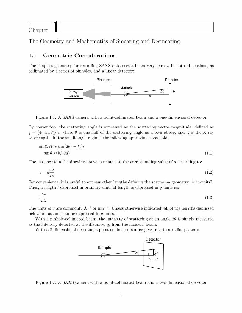
The simplest geometry for recording SAXS data uses a beam very narrow in both dimensions, ascollimated by a series of pinholes, and a linear detector:
X-ray
Source
Pinholes
Sample
Detector
2θ
a
b
Figure 1.1: A SAXS camera with a point-collimated beam and a one-dimensional detector
By convention, the scattering angle is expressed as the scattering vector magnitude, defined asq = (4π sin θ)/λ, where θ is one-half of the scattering angle as shown above, and λ is the X-raywavelength. In the small-angle regime, the following approximations hold:
sin(2θ) ≈ tan(2θ) = b/a
sin θ ≈ b/(2a) (1.1)
The distance b in the drawing above is related to the corresponding value of q according to:
b = qaλ
2π(1.2)
For convenience, it is useful to express other lengths defining the scattering geometry in “q-units”.Thus, a length l expressed in ordinary units of length is expressed in q-units as:
l2π
aλ(1.3)
The units of q are commonly A−1 or nm−1. Unless otherwise indicated, all of the lengths discussedbelow are assumed to be expressed in q-units.
With a pinhole-collimated beam, the intensity of scattering at an angle 2θ is simply measuredas the intensity detected at the distance, q, from the incident beam.
With a 2-dimensional detector, a point-collimated source gives rise to a radial pattern:
Sample
Detector
2θ q
Figure 1.2: A SAXS camera with a point-collimated beam and a two-dimensional detector
1
The intensity corresponding to the scattering angle 2θ is then determined by integrating over thecircle with radius q.
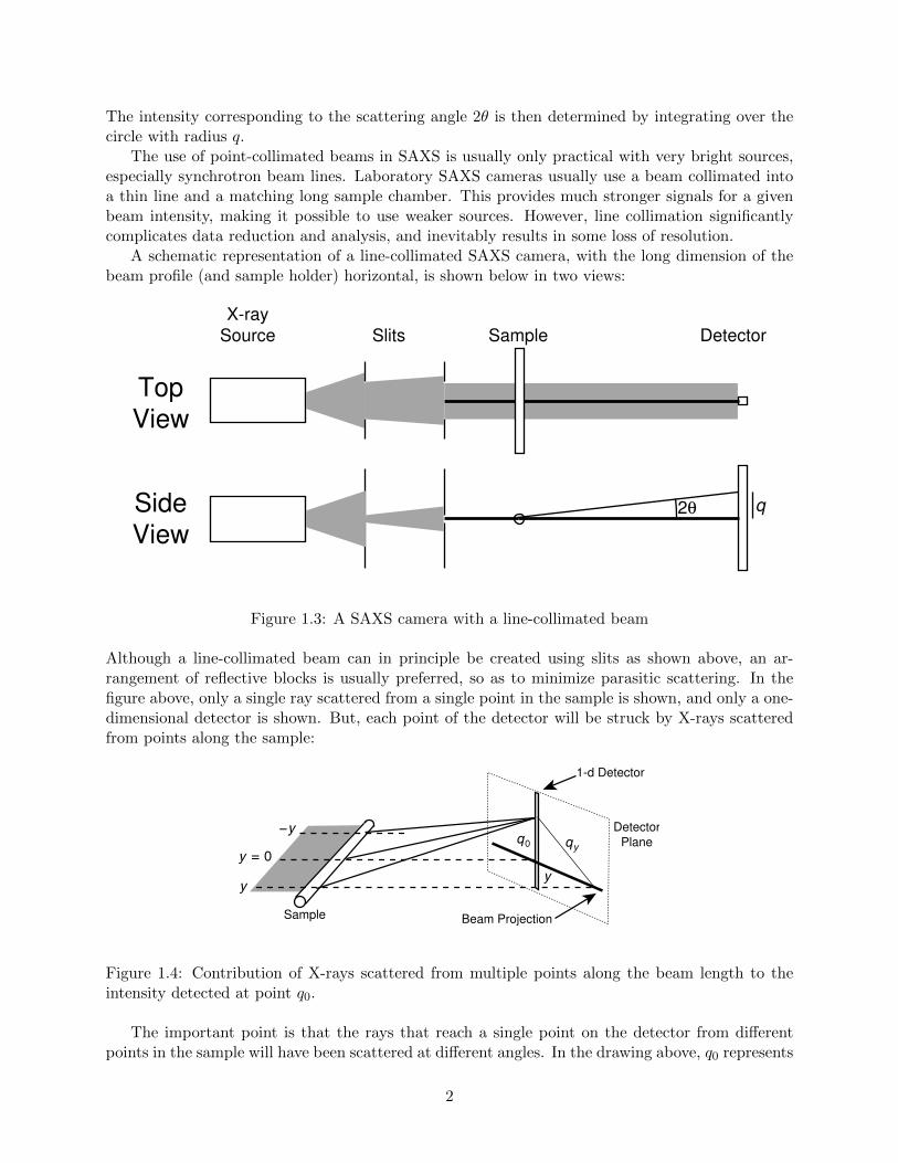
The use of point-collimated beams in SAXS is usually only practical with very bright sources,especially synchrotron beam lines. Laboratory SAXS cameras usually use a beam collimated intoa thin line and a matching long sample chamber. This provides much stronger signals for a givenbeam intensity, making it possible to use weaker sources. However, line collimation significantlycomplicates data reduction and analysis, and inevitably results in some loss of resolution.
A schematic representation of a line-collimated SAXS camera, with the long dimension of thebeam profile (and sample holder) horizontal, is shown below in two views:
X-ray
Source Slits Sample Detector
2θ q
TopView
SideView
Figure 1.3: A SAXS camera with a line-collimated beam
Although a line-collimated beam can in principle be created using slits as shown above, an ar-rangement of reflective blocks is usually preferred, so as to minimize parasitic scattering. In thefigure above, only a single ray scattered from a single point in the sample is shown, and only a one-dimensional detector is shown. But, each point of the detector will be struck by X-rays scatteredfrom points along the sample:
Sample
1-d Detector
Detector
Plane
Beam Projection
Figure 1.4: Contribution of X-rays scattered from multiple points along the beam length to theintensity detected at point q0.
The important point is that the rays that reach a single point on the detector from differentpoints in the sample will have been scattered at different angles. In the drawing above, q0 represents
2
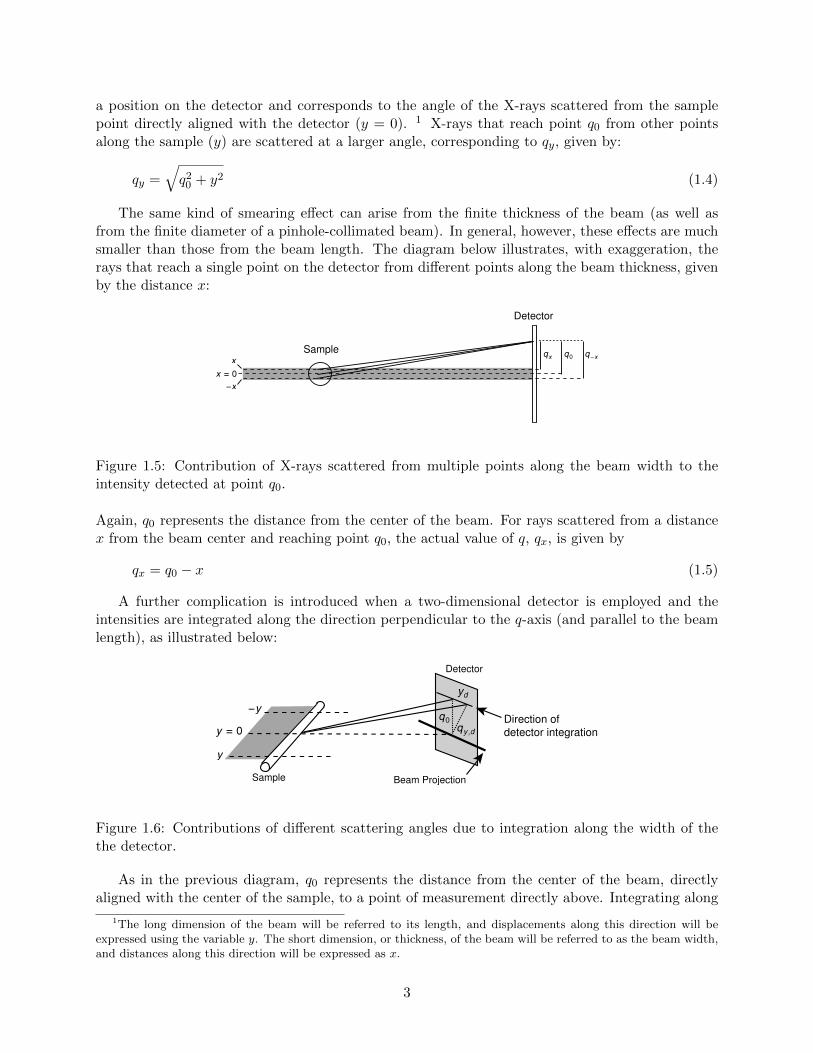
a position on the detector and corresponds to the angle of the X-rays scattered from the samplepoint directly aligned with the detector (y = 0). 1 X-rays that reach point q0 from other pointsalong the sample (y) are scattered at a larger angle, corresponding to qy, given by:
qy =√q2
0 + y2 (1.4)
The same kind of smearing effect can arise from the finite thickness of the beam (as well asfrom the finite diameter of a pinhole-collimated beam). In general, however, these effects are muchsmaller than those from the beam length. The diagram below illustrates, with exaggeration, therays that reach a single point on the detector from different points along the beam thickness, givenby the distance x:
Sample
Detector
Figure 1.5: Contribution of X-rays scattered from multiple points along the beam width to theintensity detected at point q0.
Again, q0 represents the distance from the center of the beam. For rays scattered from a distancex from the beam center and reaching point q0, the actual value of q, qx, is given by
qx = q0 − x (1.5)
A further complication is introduced when a two-dimensional detector is employed and theintensities are integrated along the direction perpendicular to the q-axis (and parallel to the beamlength), as illustrated below:
Sample
Detector
Beam Projection
Direction of
detector integration
Figure 1.6: Contributions of different scattering angles due to integration along the width of thethe detector.
As in the previous diagram, q0 represents the distance from the center of the beam, directlyaligned with the center of the sample, to a point of measurement directly above. Integrating along
1The long dimension of the beam will be referred to its length, and displacements along this direction will beexpressed using the variable y. The short dimension, or thickness, of the beam will be referred to as the beam width,and distances along this direction will be expressed as x.
3
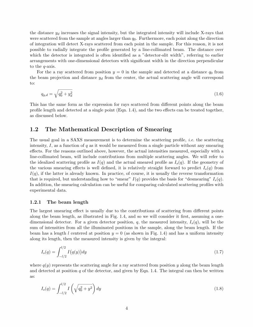
the distance yd increases the signal intensity, but the integrated intensity will include X-rays thatwere scattered from the sample at angles larger than q0. Furthermore, each point along the directionof integration will detect X-rays scattered from each point in the sample. For this reason, it is notpossible to radially integrate the profile generated by a line-collimated beam. The distance overwhich the detector is integrated is often identified as a ”detector-slit width”, referring to earlierarrangements with one-dimensional detectors with significant width in the direction perpendicularto the q-axis.
For the a ray scattered from position y = 0 in the sample and detected at a distance q0 fromthe beam projection and distance yd from the center, the actual scattering angle will correspondto:
qy,d =√q2
0 + y2d (1.6)
This has the same form as the expression for rays scattered from different points along the beamprofile length and detected at a single point (Eqn. 1.4), and the two effects can be treated together,as discussed below.
1.2 The Mathematical Description of Smearing
The usual goal in a SAXS measurement is to determine the scattering profile, i.e. the scatteringintensity, I, as a function of q as it would be measured from a single particle without any smearingeffects. For the reasons outlined above, however, the actual intensities measured, especially with aline-collimated beam, will include contributions from multiple scattering angles. We will refer tothe idealized scattering profile as I(q) and the actual smeared profile as Is(q). If the geometry ofthe various smearing effects is well defined, it is relatively straight forward to predict Is(q) fromI(q), if the latter is already known. In practice, of course, it is usually the reverse transformationthat is required, but understanding how to “smear” I(q) provides the basis for “desmearing” Is(q).In addition, the smearing calculation can be useful for comparing calculated scattering profiles withexperimental data.
1.2.1 The beam length
The largest smearing effect is usually due to the contributions of scattering from different pointsalong the beam length, as illustrated in Fig. 1.4, and so we will consider it first, assuming a one-dimensional detector. For a given detector position, q, the measured intensity, Is(q), will be thesum of intensities from all the illuminated positions in the sample, along the beam length. If thebeam has a length l centered at position y = 0 (as shown in Fig. 1.4) and has a uniform intensityalong its length, then the measured intensity is given by the integral:
Is(q) =
∫ l/2
−l/2I(q(y)
)dy (1.7)
where q(y) represents the scattering angle for a ray scattered from position y along the beam lengthand detected at position q of the detector, and given by Eqn. 1.4. The integral can then be writtenas:
Is(q) =
∫ l/2
−l/2I
(√q2
0 + y2
)dy (1.8)
4
In general, however, the beam-length profile will not have a uniform intensity, but rather will fallof gradually at each end. Eqn. 1.8 can be generalized by introducing a weighting function, w(y),and writing the integral as:
Is(q) =
∫ ∞−∞
w(y)I
(√q2
0 + y2
)dy (1.9)
The weighting function should be normalized so that:∫ ∞−∞
w(y) = 1 (1.10)
The beam-length profile is often assumed to be symmetrical about y = 0, so that Eqn. 1.9 can bewritten as:
Is(q) = 2
∫ ∞0
w(y)I
(√q2
0 + y2
)dy (1.11)
For the case of a uniform beam of length l, the weighting function is given by:
w(y) =
0 : y < −l/21/l : −l/2 ≤ y ≤ l/20 : y > l/2
(1.12)
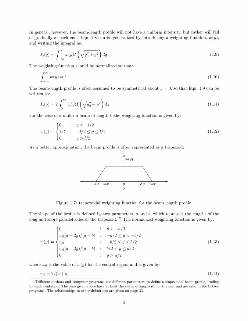
As a better approximation, the beam profile is often represented as a trapezoid:
0
Figure 1.7: trapezoidal weighting function for the beam length profile.
The shape of the profile is defined by two parameters, a and b, which represent the lengths of thelong and short parallel sides of the trapezoid. 2 The normalized weighting function is given by:
w(y) =
0 : y < −a/2w0(a+ 2y)/(a− b) : −a/2 ≤ y < −b/2w0 : −b/2 ≤ y ≤ b/2w0(a− 2y)/(a− b) : b/2 < y ≤ a/20 : y > a/2
(1.13)
where w0 is the value of w(y) for the central region and is given by:
w0 = 2/(a+ b) (1.14)
2Different authors and computer programs use different parameters to define a trapezoidal beam profile, leadingto much confusion. The ones given above have at least the virtue of simplicity for the user and are used in the USTooprograms. The relationships to other definitions are given on page 33.
5

A curvier, if not necessarily sexier, function that can be used to represent the beam lengthprofile is:
w(y) =1 + a
a+ e|y|/b(1.15)
where a and b are parameters defining the curve. As given above, the function is not normalized,but it can be normalized by multiplying be the factor w0:
w0 =a
2(1 + a) ln(1 + ab)(1.16)
A fit of this function to a measured beam profile is shown below, along with a trapezoidal approx-imation:
Figure 1.8: A fit of the sigmoidal function to a measured beam-length profile. From ImageJ withthe saxsImage plugin.
This profile function is offered as an option, along with the trapezoidal function, in the Utah SAXSTools, where it is referred to as a sigmoidal beam profile.
1.2.2 The beam width
Here, we initially consider only the effect of a finite beam width, as illustrated in Fig. 1.5, with yset to 0. If q is the distance from the detector point to the center of the beam width, then pointsabove and below the center point will also contribute to the measured intensity, with scatteringangles that depend on the position, x, relative to the beam center. The total observed intensity atthe nominal q-value will be the integral of the intensity from the points across the beam width:
Is(q) =
∫ ∞−∞
v(x)I (q −X)) dx (1.17)
where v(x) is a weighting function, analogous to w(y) for the y-direction, that describes the intensityprofile of the beam across it width. The beam-width profile can be approximated as a trapezoid oras a Gaussian function, as show below for a measured profile:
6
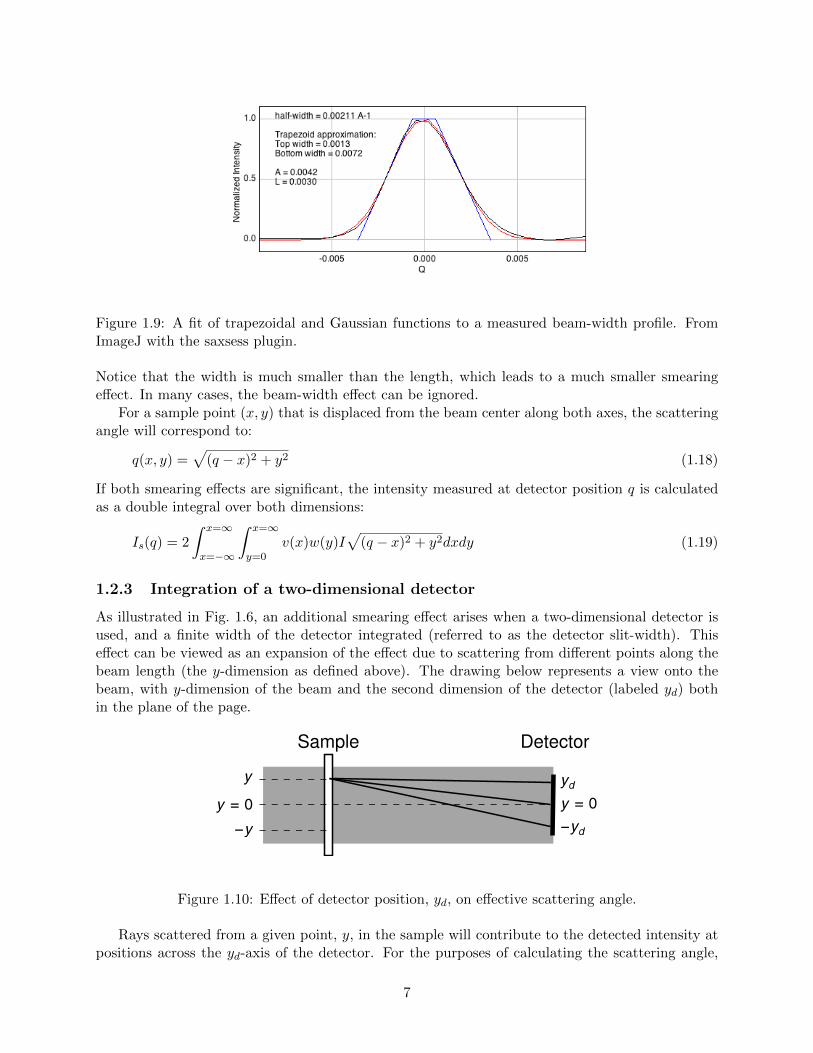
Figure 1.9: A fit of trapezoidal and Gaussian functions to a measured beam-width profile. FromImageJ with the saxsess plugin.
Notice that the width is much smaller than the length, which leads to a much smaller smearingeffect. In many cases, the beam-width effect can be ignored.
For a sample point (x, y) that is displaced from the beam center along both axes, the scatteringangle will correspond to:
q(x, y) =√
(q − x)2 + y2 (1.18)
If both smearing effects are significant, the intensity measured at detector position q is calculatedas a double integral over both dimensions:
Is(q) = 2
∫ x=∞
x=−∞
∫ x=∞
y=0v(x)w(y)I
√(q − x)2 + y2dxdy (1.19)
1.2.3 Integration of a two-dimensional detector
As illustrated in Fig. 1.6, an additional smearing effect arises when a two-dimensional detector isused, and a finite width of the detector integrated (referred to as the detector slit-width). Thiseffect can be viewed as an expansion of the effect due to scattering from different points along thebeam length (the y-dimension as defined above). The drawing below represents a view onto thebeam, with y-dimension of the beam and the second dimension of the detector (labeled yd) bothin the plane of the page.
Sample Detector
Figure 1.10: Effect of detector position, yd, on effective scattering angle.
Rays scattered from a given point, y, in the sample will contribute to the detected intensity atpositions across the yd-axis of the detector. For the purposes of calculating the scattering angle,
7
we can think of an “effective y-position” for a given actual y-position and a detector position, yd,given by:
yeff = y − yd (1.20)
One consequence is that the effective range of smeared y-values is increased by the detector width.To account for this additional effect we must, in essence, integrate over yd as well as y (and x ifthe beam width is significant).
A mathematically convenient way of incorporating the additional integration is by modifyingthe beam-length profile, w(y). For a given value of y, the new weighting function, W (y), is givenby:
W (y) =
∫ ld/2
−ld/2w(y − yd)dyd (1.21)
where l/d is the length of the segment integrated on the detector. This equation represents aconvolution of w(y) by a square pulse function (representing the detector segment length) and hasthe net effect of broadening w(x).
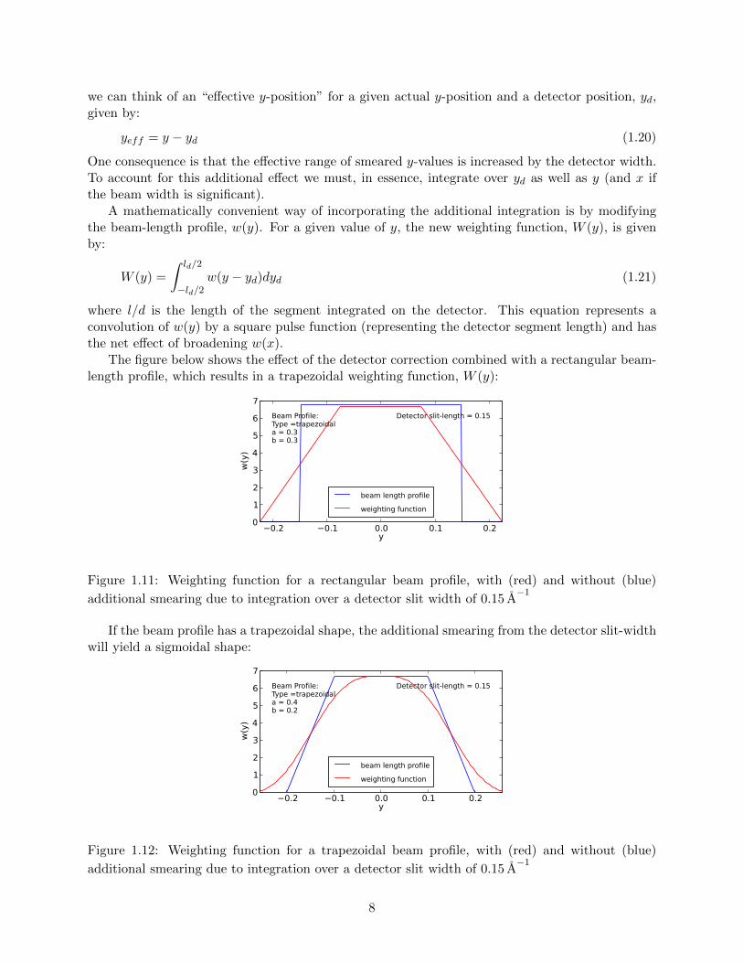
The figure below shows the effect of the detector correction combined with a rectangular beam-length profile, which results in a trapezoidal weighting function, W (y):
Figure 1.11: Weighting function for a rectangular beam profile, with (red) and without (blue)
additional smearing due to integration over a detector slit width of 0.15 A−1
If the beam profile has a trapezoidal shape, the additional smearing from the detector slit-widthwill yield a sigmoidal shape:
Figure 1.12: Weighting function for a trapezoidal beam profile, with (red) and without (blue)
additional smearing due to integration over a detector slit width of 0.15 A−1
8
Finally, the effect on a sigmoidal beam profile is shown below:
Figure 1.13: Weighting function for a sigmoidal beam profile, with (red) and without (blue) addi-
tional smearing due to integration over a detector slit width of 0.15 A−1
1.2.4 Some simulated examples
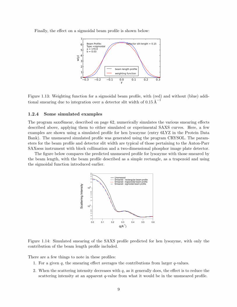
The program saxsSmear, described on page 62, numerically simulates the various smearing effectsdescribed above, applying them to either simulated or experimental SAXS curves. Here, a fewexamples are shown using a simulated profile for hen lysozyme (entry 6LYZ in the Protein DataBank). The unsmeared simulated profile was generated using the program CRYSOL. The param-eters for the beam profile and detector slit width are typical of those pertaining to the Anton-ParrSAXsess instrument with block collimation and a two-dimensional phosphor image plate detector.
The figure below compares the predicted unsmeared profile for lysozyme with those smeared bythe beam length, with the beam profile described as a simple rectangle, as a trapezoid and usingthe sigmoidal function introduced earlier.
2
3
4
56
105
2
3
456
106
2
3
4
56
Scattering Inte
nsity
0.60.50.40.30.20.10.0
q(A-1
)
Unsmeared Smeared - rectangular beam profile Smeared - trapezoidal beam profile Smeared - sigmoidal beam profile
Figure 1.14: Simulated smearing of the SAXS profile predicted for hen lysozyme, with only thecontribution of the beam length profile included.
There are a few things to note in these profiles:
1. For a given q, the smearing effect averages the contributions from larger q-values.
2. When the scattering intensity decreases with q, as it generally does, the effect is to reduce thescattering intensity at an apparent q-value from what it would be in the unsmeared profile.
9
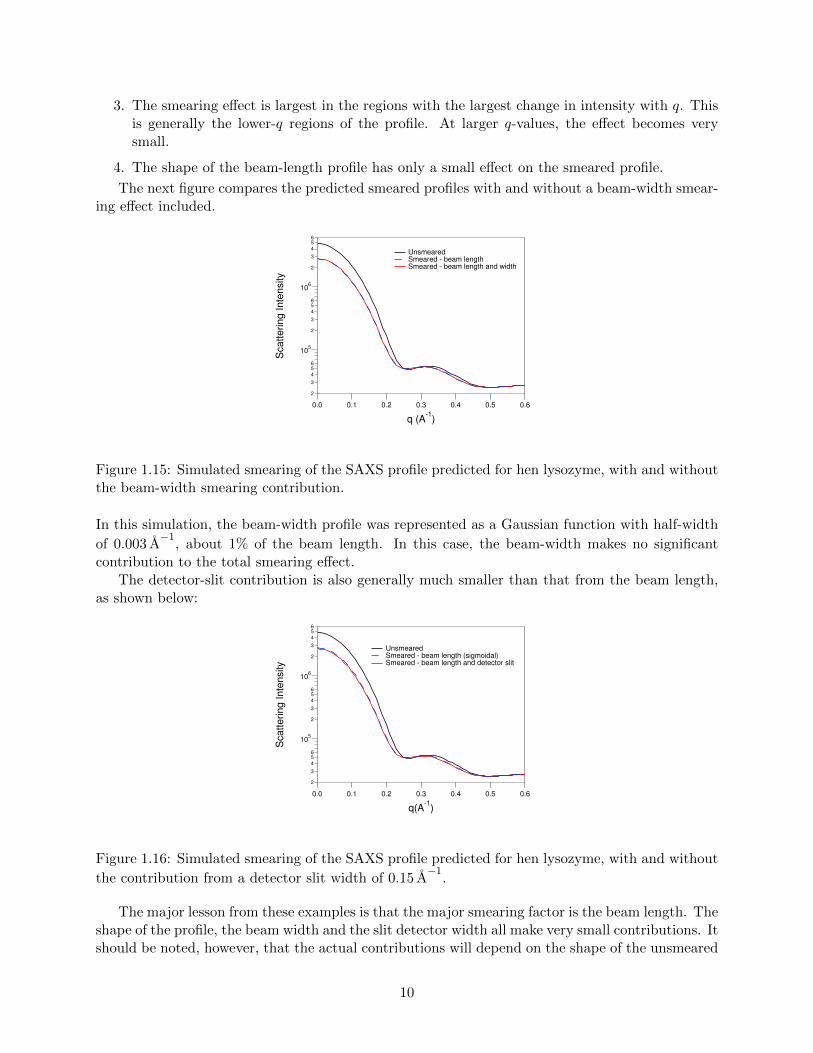
3. The smearing effect is largest in the regions with the largest change in intensity with q. Thisis generally the lower-q regions of the profile. At larger q-values, the effect becomes verysmall.
4. The shape of the beam-length profile has only a small effect on the smeared profile.
The next figure compares the predicted smeared profiles with and without a beam-width smear-ing effect included.
2
3
4
56
105
2
3
456
106
2
3
4
56
Scattering Inte
nsity
0.60.50.40.30.20.10.0
q (A-1
)
Unsmeared Smeared - beam length Smeared - beam length and width
Figure 1.15: Simulated smearing of the SAXS profile predicted for hen lysozyme, with and withoutthe beam-width smearing contribution.
In this simulation, the beam-width profile was represented as a Gaussian function with half-width
of 0.003 A−1
, about 1% of the beam length. In this case, the beam-width makes no significantcontribution to the total smearing effect.
The detector-slit contribution is also generally much smaller than that from the beam length,as shown below:
2
3
4
56
105
2
3
456
106
2
3
4
56
Scattering Inte
nsity
0.60.50.40.30.20.10.0
q(A-1
)
Unsmeared Smeared - beam length (sigmoidal) Smeared - beam length and detector slit
Figure 1.16: Simulated smearing of the SAXS profile predicted for hen lysozyme, with and without
the contribution from a detector slit width of 0.15 A−1
.
The major lesson from these examples is that the major smearing factor is the beam length. Theshape of the profile, the beam width and the slit detector width all make very small contributions. Itshould be noted, however, that the actual contributions will depend on the shape of the unsmeared
10
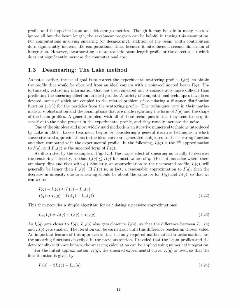
profile and the specific beam and detector geometries. Though it may be safe in many cases toignore all but the beam length, the saxsSmear program can be helpful in testing this assumption.For computations involving smearing (or desmearing), addition of the beam width contributiondoes significantly increase the computational time, because it introduces a second dimension ofintegration. However, incorporating a more realistic beam-length profile or the detector slit widthdoes not significantly increase the computational cost.
1.3 Desmearing: The Lake method
As noted earlier, the usual goal is to correct the experimental scattering profile, Is(q), to obtainthe profile that would be obtained from an ideal camera with a point-collimated beam I(q). Un-fortunately, extracting information that has been smeared out is considerably more difficult thanpredicting the smearing effect on an ideal profile. A variety of computational techniques have beendevised, some of which are coupled to the related problem of calculating a distance distributionfunction (p(r)) for the particles from the scattering profile. The techniques vary in their mathe-matical sophistication and the assumptions that are made regarding the form of I(q) and the shapeof the beam profiles. A general problem with all of these techniques is that they tend to be quitesensitive to the noise present in the experimental profile, and they usually increase the noise.
One of the simplest and most widely used methods is an iterative numerical technique introducedby Lake in 1967. Lake’s treatment begins by considering a general iterative technique in whichsuccessive trial approximations to the ideal curve are generated, subjected to the smearing functionand then compared with the experimental profile. In the following, Ii(q) is the ith approximationto I(q), and Ii,s(q) is the smeared form of Ii(q).
As illustrated by the example in Fig. 1.14, the major effect of smearing us usually to decreasethe scattering intensity, so that Is(q) ≤ I(q) for most values of q. (Exceptions arise where thereare sharp dips and rises with q.) Similarly, an approximation to the unsmeared profile, Ii(q), willgenerally be larger than Ii,s(q). If Ii(q) is, in fact, a reasonable approximation to I(q), then thedecrease in intensity due to smearing should be about the same for for I(q) and Ii(q), so that wecan write:
I(q)− Is(q) ≈ Ii(q)− Ii,s(q)I(q) ≈ Is(q) +
(Ii(q)− Ii,s(q)
)(1.22)
This then provides a simple algorithm for calculating successive approximations:
Ii+1(q) = Ii(q) + Is(q)− Ii,s(q) (1.23)
As Ii(q) gets closer to I(q), Ii,s(q) also gets closer to Is(q), so that the difference between Ii+1(q)and Ii(q) gets smaller. The iteration can be carried out until this difference reaches an chosen value.An important feature of this approach is that the only required mathematical transformations arethe smearing functions described in the previous section. Provided that the beam profiles and thedetector slit-width are known, the smearing calculation can be applied using numerical integration.
For the initial approximation, I1(q), the smeared experimental curve, Is(q) is used, so that thefirst iteration is given by:
I1(q) = 2Is(q)− Is,s(q) (1.24)
11
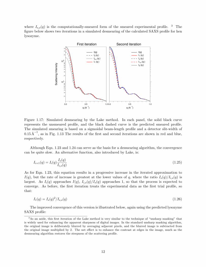
where Is,s(q) is the computationally-smeared form of the smeared experimental profile. 3 Thefigure below shows two iterations in a simulated desmearing of the calculated SAXS profile for henlysozyme.
1.00.50.0
q (A-1
)
2
3
4
5
678
105
2
3
4
5
678
106
2
3
4
Sca
tte
rin
g I
nte
nsity
1.00.50.0
q (A-1
)
I(q)
I1 (q )
Is (q )
I1,s (q )
I2 (q )
I(q)
Is (q )
Is,s (q )
I1 (q )
First iteration Second iteration
Figure 1.17: Simulated desmearing by the Lake method. In each panel, the solid black curverepresents the unsmeared profile, and the black dashed curve is the predicted smeared profile.The simulated smearing is based on a sigmoidal beam-length profile and a detector slit-width of
0.15 A−1
, as in Fig. 1.13 The results of the first and second iterations are shown in red and blue,respectively.
Although Eqn. 1.23 and 1.24 can serve as the basis for a desmearing algorithm, the convergencecan be quite slow. An alternative function, also introduced by Lake, is:
Ii+1(q) = Ii(q)Is(q)
Ii,s(q)(1.25)
As for Eqn. 1.23, this equation results in a progressive increase in the iterated approximation toI(q), but the rate of increase is greatest at the lower values of q, where the ratio Is(q)/Ii,s(q) islargest. As Ii(q) approaches I(q), Ii,s(q)/Is(q) approaches 1, so that the process is expected toconverge. As before, the first iteration treats the experimental data as the first trial profile, sothat:
I1(q) = Is(q)2/Is,s(q) (1.26)
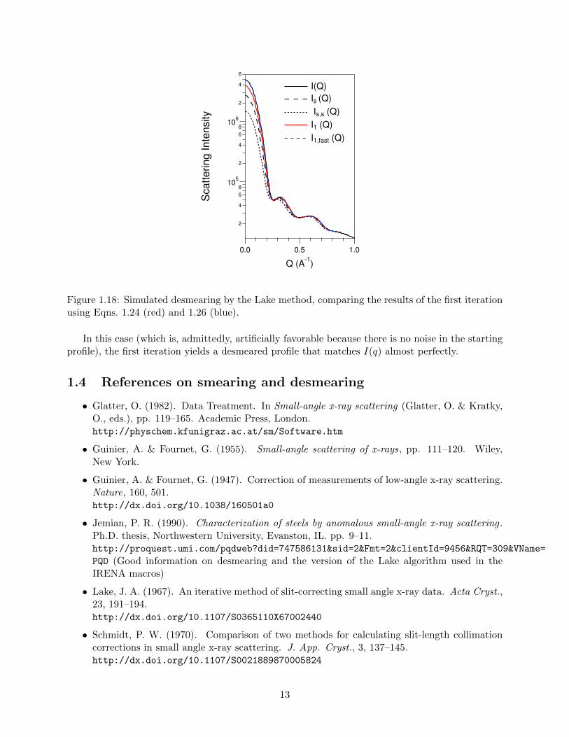
The improved convergence of this version is illustrated below, again using the predicted lysozymeSAXS profile:
3As an aside, this first iteration of the Lake method is very similar to the technique of “unsharp masking” thatis widely used for enhancing the apparent sharpness of digital images. In the standard unsharp masking algorithm,the original image is deliberately blurred by averaging adjacent pixels, and the blurred image is subtracted fromthe original image multiplied by 2. The net effect is to enhance the contrast at edges in the image, much as thedesmearing algorithm restores the steepness of the scattering profile.
12
2
4
6
810
5
2
4
6
810
6
2
4
6
Scattering Inte
nsity
1.00.50.0
Q (A-1
)
I(Q)
Is (Q)
Is,s (Q)
I1 (Q)
I1,fast (Q)
Figure 1.18: Simulated desmearing by the Lake method, comparing the results of the first iterationusing Eqns. 1.24 (red) and 1.26 (blue).
In this case (which is, admittedly, artificially favorable because there is no noise in the startingprofile), the first iteration yields a desmeared profile that matches I(q) almost perfectly.
1.4 References on smearing and desmearing
• Glatter, O. (1982). Data Treatment. In Small-angle x-ray scattering (Glatter, O. & Kratky,O., eds.), pp. 119–165. Academic Press, London.http://physchem.kfunigraz.ac.at/sm/Software.htm
• Guinier, A. & Fournet, G. (1955). Small-angle scattering of x-rays, pp. 111–120. Wiley,New York.
• Guinier, A. & Fournet, G. (1947). Correction of measurements of low-angle x-ray scattering.Nature, 160, 501.http://dx.doi.org/10.1038/160501a0
• Jemian, P. R. (1990). Characterization of steels by anomalous small-angle x-ray scattering .Ph.D. thesis, Northwestern University, Evanston, IL. pp. 9–11.http://proquest.umi.com/pqdweb?did=747586131&sid=2&Fmt=2&clientId=9456&RQT=309&VName=
PQD (Good information on desmearing and the version of the Lake algorithm used in theIRENA macros)
• Lake, J. A. (1967). An iterative method of slit-correcting small angle x-ray data. Acta Cryst.,23, 191–194.http://dx.doi.org/10.1107/S0365110X67002440
• Schmidt, P. W. (1970). Comparison of two methods for calculating slit-length collimationcorrections in small angle x-ray scattering. J. App. Cryst., 3, 137–145.http://dx.doi.org/10.1107/S0021889870005824
13
Chapter 2Absolute Scattering Intensities and Determination of Molecular Weights
For many purposes, it is sufficient to measure and report scattering intensities in arbitrary units, asmuch of the information from SAXS is derived from the shape of the scattering profile. However,the absolute intensities can be used to determine the molecular weight of a scattering particle, oralternatively the concentration of particles if the molecular weight is known, and can also be ofvalue in comparing experimental and theoretical profiles.
The units of scattering intensity and their interpretation can be quite confusing. The expression“absolute intensity” is used in at least two different ways, but of which are a bit misleading. Anotherpossible source of confusion is that the scattering community generally uses the older cgs systemof units, rather than SI units, a convention that is followed here.
2.1 The microscopic differential scattering cross section
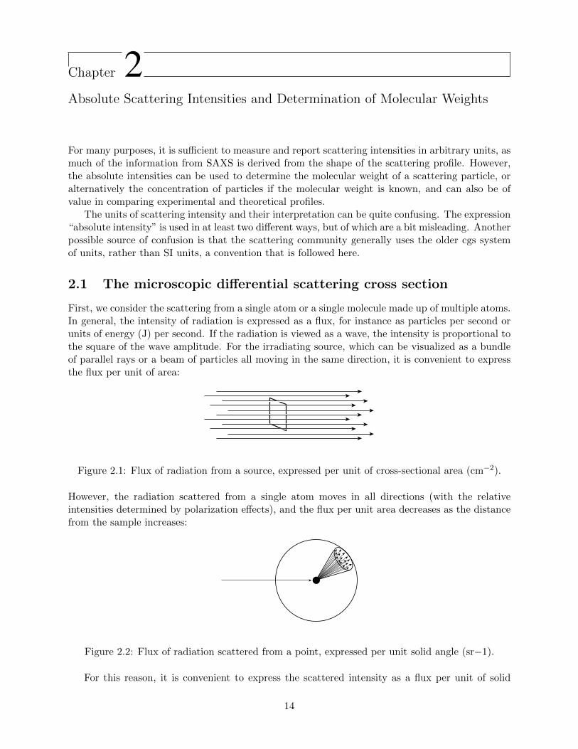
First, we consider the scattering from a single atom or a single molecule made up of multiple atoms.In general, the intensity of radiation is expressed as a flux, for instance as particles per second orunits of energy (J) per second. If the radiation is viewed as a wave, the intensity is proportional tothe square of the wave amplitude. For the irradiating source, which can be visualized as a bundleof parallel rays or a beam of particles all moving in the same direction, it is convenient to expressthe flux per unit of area:
Figure 2.1: Flux of radiation from a source, expressed per unit of cross-sectional area (cm−2).
However, the radiation scattered from a single atom moves in all directions (with the relativeintensities determined by polarization effects), and the flux per unit area decreases as the distancefrom the sample increases:
Figure 2.2: Flux of radiation scattered from a point, expressed per unit solid angle (sr−1).
For this reason, it is convenient to express the scattered intensity as a flux per unit of solid
14
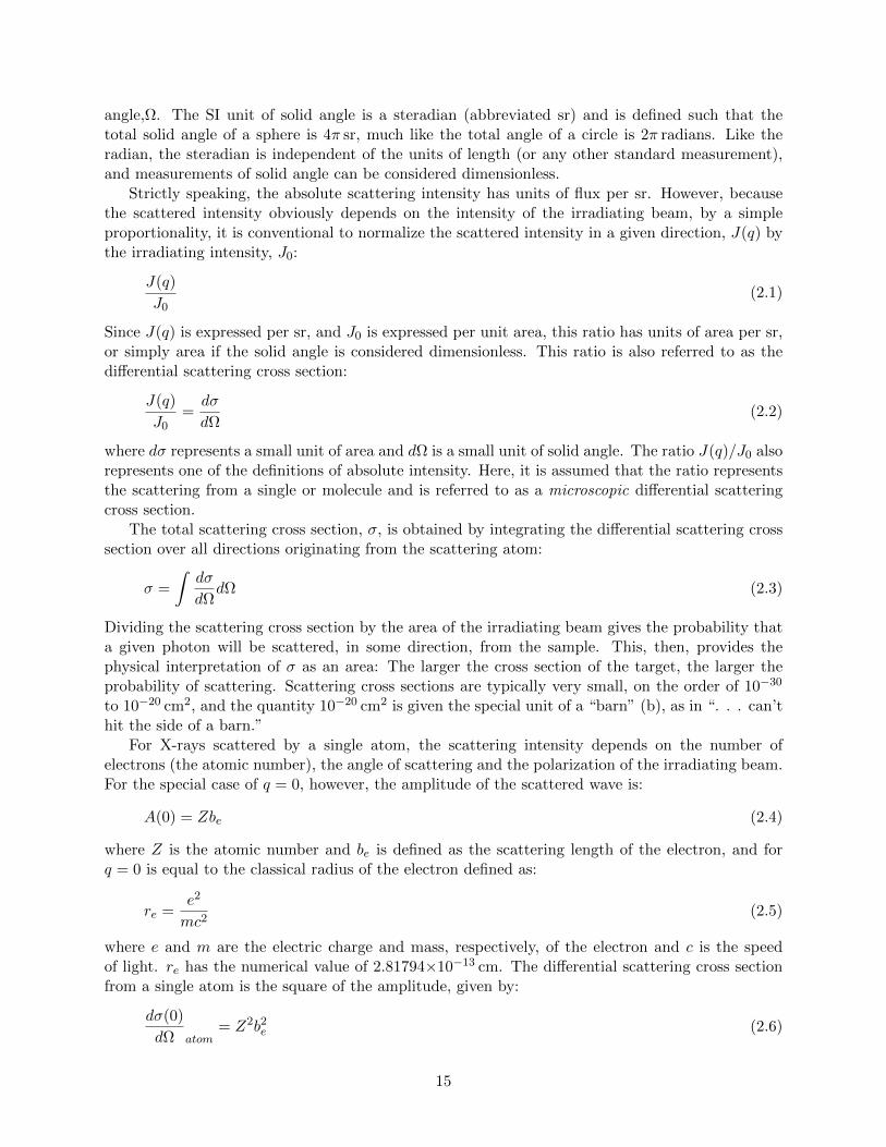
angle,Ω. The SI unit of solid angle is a steradian (abbreviated sr) and is defined such that thetotal solid angle of a sphere is 4π sr, much like the total angle of a circle is 2π radians. Like theradian, the steradian is independent of the units of length (or any other standard measurement),and measurements of solid angle can be considered dimensionless.
Strictly speaking, the absolute scattering intensity has units of flux per sr. However, becausethe scattered intensity obviously depends on the intensity of the irradiating beam, by a simpleproportionality, it is conventional to normalize the scattered intensity in a given direction, J(q) bythe irradiating intensity, J0:
J(q)
J0(2.1)
Since J(q) is expressed per sr, and J0 is expressed per unit area, this ratio has units of area per sr,or simply area if the solid angle is considered dimensionless. This ratio is also referred to as thedifferential scattering cross section:
J(q)
J0=dσ
dΩ(2.2)
where dσ represents a small unit of area and dΩ is a small unit of solid angle. The ratio J(q)/J0 alsorepresents one of the definitions of absolute intensity. Here, it is assumed that the ratio representsthe scattering from a single or molecule and is referred to as a microscopic differential scatteringcross section.
The total scattering cross section, σ, is obtained by integrating the differential scattering crosssection over all directions originating from the scattering atom:
σ =
∫dσ
dΩdΩ (2.3)
Dividing the scattering cross section by the area of the irradiating beam gives the probability thata given photon will be scattered, in some direction, from the sample. This, then, provides thephysical interpretation of σ as an area: The larger the cross section of the target, the larger theprobability of scattering. Scattering cross sections are typically very small, on the order of 10−30
to 10−20 cm2, and the quantity 10−20 cm2 is given the special unit of a “barn” (b), as in “. . . can’thit the side of a barn.”
For X-rays scattered by a single atom, the scattering intensity depends on the number ofelectrons (the atomic number), the angle of scattering and the polarization of the irradiating beam.For the special case of q = 0, however, the amplitude of the scattered wave is:
A(0) = Zbe (2.4)
where Z is the atomic number and be is defined as the scattering length of the electron, and forq = 0 is equal to the classical radius of the electron defined as:
re =e2
mc2(2.5)
where e and m are the electric charge and mass, respectively, of the electron and c is the speedof light. re has the numerical value of 2.81794×10⁻¹³ cm. The differential scattering cross sectionfrom a single atom is the square of the amplitude, given by:
dσ(0)
dΩ atom= Z2b2e (2.6)
15
For a molecule, the X-ray scattering at a given angle depends on the interference of wavesscattered from the individual atoms, in addition to the factors mentioned above, but at q = 0,the scattering amplitude is the simple sum of the amplitudes from the individual atoms, and theintensity is the square of this sum:
dσ(0)
dΩ m=
(N∑i=1
Zibe
)2
(2.7)
where N is the total number of atoms in the molecule and Zi is the atomic number of atom i.For neutron scattering, the scattering length of each atom depends on the properties of the
individual nuclear types, but the total scattering is determined by an analogous sum of the ampli-tudes.
2.2 The macroscopic differential scattering cross section
The scattering from a macroscopic sample reflects both the total scattering intensity from all of themolecules and possible interference effects from waves scattered from different molecules. In thelimit of high dilution, the effects of interparticle interference can be ignored and the total intensityis the sum of the scattering from the individual molecules. Ignoring, for the moment, the effects ofsolvent displaced by the molecules, the total scattering can be written as:
J(q)
J0= Nm
dσ
dΩm(2.8)
where Nm is the number of molecules in the irradiated volume. This volume depends on both thecross-sectional area of the beam (or that part of the beam that passes through the sample if thebeam cross section is smaller than the sample) and the length of the sample. The cross sectionof the beam is already accounted for in the definition of the scattering cross section (and leadsto the units of area), but the sample length is not. Since the irradiated volume can vary fromone instrument to another, even if the sample concentrations are accounted for, it is convenient toexpress scattering intensities per unit volume:
J(q)
J0
1
Vs=Nm
Vs
dσ
dΩm(2.9)
where Vs is the sample volume. This quantity is defined as the macroscopic differential scatteringcross section:
dΣ
dΩ=Nm
Vs
dσ
dΩm(2.10)
The ratio (Nm/Vs) is the number density of molecules in the sample. Importantly, dΣdΩ is a property
of the sample (reflecting the concentration of scattering molecules) and should be independent ofexperimental details such as sample volume, beam intensity, detector efficiency, etc.. The unitsof this quantity are cm−1, and it can be thought of as representing the dimensionless scatteringfrom a sample 1 cm long, after correcting for the flux per unit area of the irradiating beam. Themacroscopic differential scattering cross section is the more widely used definition of “absolutescattering intensity”, and this definition will be used here.
16
2.3 Contrast for a solution sample
When SAXS profiles for solution samples are measured, the usual practice is to subtract the signalfrom a carefully matched reference sample containing everything but the macromolecules of interest.The resulting difference profile represents the differences between the amplitudes of the wavesscattered from the macromolecule and those scattered from the solvent molecules displaced by themacromolecule. Importantly, it is the difference in wave amplitudes, rather than intensities, thatmust be accounted for.
The total amplitude from an isolated molecule, at q = 0, is the sum of the atomic scatteringlengths:
A(0)m =
N∑i=1
Zibe (2.11)
where Zi is the atomic number of the ith atom.For the solvent, it is convenient to introduce a scattering density, ρsolv, which is the sum of the
electron scattering lengths, be, per unit volume. The total scattering length is then the product ofthe density and the volume displaced by the macromolecule. The volume is given by the productof the molecular mass, Mm, and the partial specific volume, v, which is the amount the solutionvolume increases with the addition of solute molecules, per gram of solute. For one molecule, thevolume is:
Vm = Mmv
= (M/NA)v (2.12)
where M is the molar mass, and NA is Avogadro’s number. The scattering amplitude (at q = 0)from the displaced solvent is then:
A(0)solv = (M/NA)vρsolv (2.13)
The scattering amplitude at q = 0 for the macromolecule can be similarly expressed in termsof a scattering density:
A(0)solv = (M/NA)vρm (2.14)
where ρm is given by
ρm =NA
∑Ni=1 ZibeMv
(2.15)
The scattering amplitude difference is then given by:
∆A(0) = (M/NA)vρm − (M/NA)vρsolv
= (M/NA)v(ρm − ρsolv) (2.16)
The net differential scattering cross section at q = 0 is given by the square of the amplitudedifference:
dσ(0)
dΩ net= ∆A(0)2
= ((M/NA)v(ρm − ρsolv))2 (2.17)
17
The macroscopic differential scattering cross section (absolute scattering intensity) is:
dΣ(0)
dΩ=Nm
Vs
dσ(0)
dΩ m(2.18)
The number density of molecules (Nm/Vs) can be expressed in terms of the mass concentration, cin g/cm3, according to:
Nm/Vs = cNA/M, (2.19)
so that the absolute scattering intensity is given by:
dΣ(0)
dΩ= (cNA/M)
dσ(0)
dΩ
= (cNA/M) ((M/NA)v(ρm − ρsolv))2
= (cM/NA)v2(ρm − ρsolv)2 (2.20)
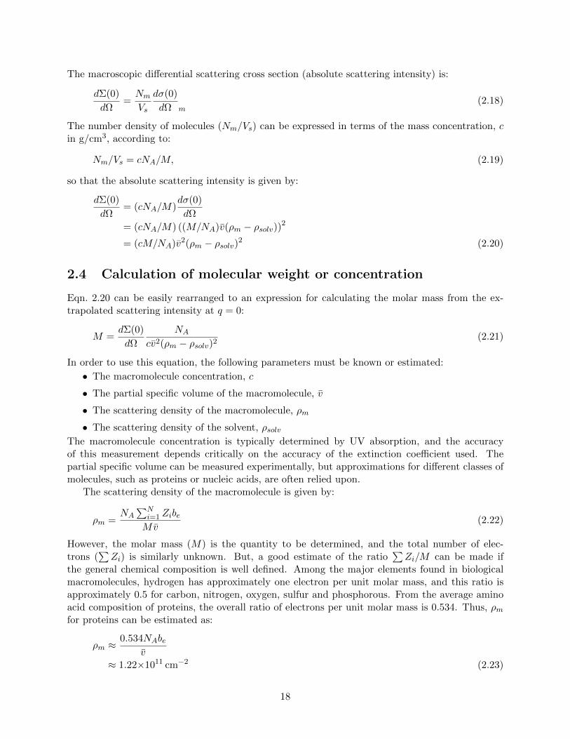
2.4 Calculation of molecular weight or concentration
Eqn. 2.20 can be easily rearranged to an expression for calculating the molar mass from the ex-trapolated scattering intensity at q = 0:
M =dΣ(0)
dΩ
NA
cv2(ρm − ρsolv)2(2.21)
In order to use this equation, the following parameters must be known or estimated:
• The macromolecule concentration, c
• The partial specific volume of the macromolecule, v
• The scattering density of the macromolecule, ρm
• The scattering density of the solvent, ρsolvThe macromolecule concentration is typically determined by UV absorption, and the accuracyof this measurement depends critically on the accuracy of the extinction coefficient used. Thepartial specific volume can be measured experimentally, but approximations for different classes ofmolecules, such as proteins or nucleic acids, are often relied upon.
The scattering density of the macromolecule is given by:
ρm =NA
∑Ni=1 ZibeMv
(2.22)
However, the molar mass (M) is the quantity to be determined, and the total number of elec-trons (
∑Zi) is similarly unknown. But, a good estimate of the ratio
∑Zi/M can be made if
the general chemical composition is well defined. Among the major elements found in biologicalmacromolecules, hydrogen has approximately one electron per unit molar mass, and this ratio isapproximately 0.5 for carbon, nitrogen, oxygen, sulfur and phosphorous. From the average aminoacid composition of proteins, the overall ratio of electrons per unit molar mass is 0.534. Thus, ρmfor proteins can be estimated as:
ρm ≈0.534NAbe
v≈ 1.22×1011 cm−2 (2.23)
18
This simple approximation ignores the contributions of a hydration layer, which is generally believedto have a scattering density intermediate between that of a protein and bulk water.
The scattering density of the solvent can similarly be estimated from its chemical structureand density. For water, the number of electrons per molecule is 10, and the average molar mass isMsolv ≈ 18.015 g/mol. If the mass density is ρsolv,m ≈ 1 g/cm3, then the scattering density can becalculated as:
ρsolv = 10beρsolv,mNA/Msolv
≈ 9.4×1010 cm−2 (2.24)
More precise values can be obtained by accounting for the temperature dependence of the densityof water (See page 22).
If the molecular mass of the macromolecule is known with confidence, then the concentrationcan be calculated by rearranging Eqn. 2.20 to a slightly different form:
c =dΣ(0)
dΩ
NA
Mv2(ρm − ρsolv)2(2.25)
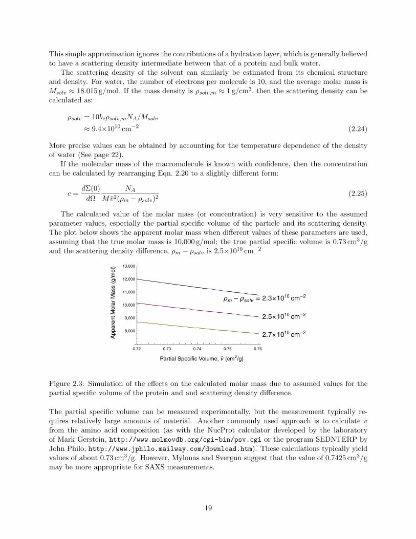
The calculated value of the molar mass (or concentration) is very sensitive to the assumedparameter values, especially the partial specific volume of the particle and its scattering density.The plot below shows the apparent molar mass when different values of these parameters are used,assuming that the true molar mass is 10,000 g/mol; the true partial specific volume is 0.73 cm3/gand the scattering density difference, ρm − ρsolv is 2.5×1010 cm−2
8,000
10,000
12,000
9,000
11,000
0.760.72 0.73 0.74 0.75
13,000
Figure 2.3: Simulation of the effects on the calculated molar mass due to assumed values for thepartial specific volume of the protein and and scattering density difference.
The partial specific volume can be measured experimentally, but the measurement typically re-quires relatively large amounts of material. Another commonly used approach is to calculate vfrom the amino acid composition (as with the NucProt calculator developed by the laboratoryof Mark Gerstein, http://www.molmovdb.org/cgi-bin/psv.cgi or the program SEDNTERP byJohn Philo, http://www.jphilo.mailway.com/download.htm). These calculations typically yieldvalues of about 0.73 cm3/g. However, Mylonas and Svergun suggest that the value of 0.7425 cm3/gmay be more appropriate for SAXS measurements.
19
2.5 Calibration of “absolute” scattering intensities
As defined on page 16, the macroscopic scattering cross-section is related to the experimentalparameters according to:
dΣ
dΩ=J(q)
J0
1
Vs(2.26)
where J(q) is the scattering flux, J0 is the incident beam flux, and Vs is the irradiated volume.Although all three of these parameters are, in principle, directly measurable, measurement of boththe incident and scattering fluxes on the same absolute scale is often not practical. An alternativeis to measure the scattered flux from a reference sample for which dΣ
dΩ is known. Different referencematerials have been used for different types of scattering experiments, but liquid reference samplesare particularly convenient for calibrating measurements with other liquids, since the cell dimensionscan be implicitly accounted for. Pure liquids have the further advantage that their scattering atrelatively low q-values arises only from thermal fluctuations. This intensity is nearly independentof q and can be calculated from macroscopic properties of the liquid, according to the relationship:
dΣ
dΩ= ρ2kTβT (2.27)
where ρ and βT are the scattering density and the isothermal compressibility of the liquid, respec-tively, k is the Boltzmann constant and T is the temperature. A significant drawback to the useof pure liquids as calibration references is that the scattering intensity is relatively weak, whichhas limited their use historically. However, with either a very bright source or a line-collimatedinstrument combined with a very sensitive detector, calibration with a pure liquid becomes quitepractical. The use of a semi-transparent beam stop, as in the Anton Par SAXSess instrument, makesthis approach particularly convenient, because the effects of sample absorption can be corrected forautomatically, as discussed below.
Calibration of absolute scattering intensities also requires corrections for the scattering due tothe capillary, as well as absorption of X-rays by the sample and references. Bulk samples giverise to significant absorption of X-rays, analogous to the absorption measured by a UV-visiblespectrophotometer. The fraction of energy absorbed by the sample is not available for scattering,so that the actual incident intensity is less that of the beam. The fraction absorbed is usually muchgreater than the fraction of energy scattered, so that the latter can be ignored, and the absorptioncan be measured by comparing the beam intensity with the intensity of X-rays that pass directlythrough the sample. The transmission, Ts, is the fraction of X-ray intensity that is not absorbedby the sample. (For simplicity and consistency with other sources, T is used here to represent bothtransmission and temperature, but never in the same equation!)
With the transmission accounted for, the actual scattering intensity, relative to the beam in-tensity, becomes:
J
J0= TsVs
dΣ
dΩ(2.28)
where Vs is the sample volume. In the SAXSess instrument, the X-ray beam stop is semi-transparentand allows a greatly attenuated profile of the beam to reach the detector. If the scattering pro-files are normalized with respect to the attenuated beam intensity, the resulting intensities areproportional to J/(TsJ0), and we can write:
I ′ = CFdΣ
dΩ(2.29)
20
where I ′ is the normalized intensity, and CF is introduced as a calibration factor that accounts forthe sample volume, incident beam intensity and the attenuation factor for the beam stop, all ofwhich are instrumental parameters. The transmission, Ts, is not included in the calibration factor,but is accounted for in the normalized intensity. To determine the calibration factor, scatteringdata are recorded for both an empty cell and the cell filled with water. The normalized intensityfrom the cell is given by:
I ′c = CFdΣ
dΩ c(2.30)
where the subscript c indicates the empty cell. Similarly, the normalized intensity from the water-filled cell is:
I ′c+w = CF
(dΣ
dΩ c+dΣ
dΩw
)(2.31)
The difference between the two normalized intensities is:
I ′c+w − I ′c = CF
(dΣ
dΩ c+dΣ
dΩw
)− CF dΣ
dΩ c(2.32)
= CFdΣ
dΩw(2.33)
and the calibration factor is calculated as:
CF =(I ′c+w − I ′c
)÷ dΣ
dΩw(2.34)
Since the intensities are normalized, and dimensionless, the calibration factor has units of cm.Once determined, the calibration factor can be applied to the normalized scattering intensities
for other samples, provided that the instrument parameters, including the irradiated sample volumeand beam geometry, are unchanged. Typically, scattering is measured for a sample containing themacromolecules of interest and a reference sample containing the same buffer. After normalization,the intensity from the sample is given by:
I ′m+b = CF
(dΣ
dΩm+dΣ
dΩ b
)(2.35)
where m and b in the subscripts represent the macromolecule and buffer contributions, respectively.The scattering from the buffer sample is:
I ′b = CFdΣ
dΩ b(2.36)
and the difference is:
I ′m+b − I ′b = CFdΣ
dΩm(2.37)
The absolute scattering intensity is then calculated as:
dΣ
dΩm= (I ′m+b − I ′b)÷ CF (2.38)
21
2.5.1 Absolute scattering of water
Though other liquids have been used as SAXS calibration standards, water offers the obviousadvantage of ready availability, and its physical properties have been well characterized over a rangeof temperatures. The two parameters that are necessary to calculate the macroscopic differentialscattering cross section are the scattering density ρ and the compressibility βT . The scatteringdensity can be calculated from the mass density, ρm, according to Eqn. 2.24. If the compressibilityis specified in units of Pa−1 and k in units of J/K, the absolute scattering intensity of water, inunits of cm−1, is calculated as:
dΣ
dΩ= ρ2kTβT (2.39)
= 10−6
(ρmNabeM
)2
kTβT (2.40)
where M is the molar mass of water and be is the electron scattering length. The factor of 10−1
arises because of the conversion from SI units to cm.Measurements and analysis by Kell (1975) provide the following expression for calculating the
mass density and compressibility of pure water. The density (in units of g/cm3) as a function oftemperature is given by:
ρm(T ) = 1×10⁻³a0 + a1T + a2T2 + a3T
3 + a4T4 + a5T
5
1 + a6T(2.41)
where the constants are: a0 = 999.83952, a1 = 16.945176, a2 = -7.9870401×10⁻³, a3 = -46.170461×10⁻⁶,a4 = 105.56302×10⁻⁹, a5 = -280.54253×10⁻¹² and a6 = 16.878950×10⁻³.
Similarly, the compressibility (in units of Pa−1) is given by:
βT (T ) = 1×10⁻¹¹a0 + a1T + a2T2 + a3T
3 + a4T4 + a5T
5
1 + a6T(2.42)
where the constants are: a0 = 50.88496, a1 = 0.6163813, a2 = 1.459187×10⁻³, a3 = 20.08438×10⁻⁶,a4 = -58.47727×10⁻⁹, a5 = 410.4110×10⁻¹² and a6 = 19.67348×10⁻³. These empirical functionsare incorporated in the USToo programs for calculating absolute scattering intensities from a waterreference.
2.6 References on calibration and molecular weight calculations
• Dreiss, C. A., Jack, K. S. & Parker, A. P. (2006). On the absolute calibration of bench-topsmall-angle X-ray scattering instruments: a comparison of different standard methods. J.App. Cryst., 39, 32–38.http://dx.doi.org/10.1107/S0021889805033091
• Kell, G. S. (1975). Density, thermal expansivity, and compressibility of liquid water from0 to 150 C: Correlations and tables for atmospheric pressure and saturation reviewed andexpressed on 1968 temperature scale. J. Chem. Eng. Data, 20, 97–105.http://dx.doi.org/10.1021/je60064a005
• Mylonas, E. & Svergun, D. (2007). Accuracy of molecular mass determination of proteins insolution by small-angle X-ray scattering. J. App. Cryst., 40, s245–s249.http://dx.doi.org/10.1107/S002188980700252X
• Orthaber, D., Bergmann, A. & Glatter, O. (2000). SAXS experiments on absolute scale withKratky systems using water as a secondary standard. J. Appl. Cryst., 33, 218–225.http://dx.doi.org/10.1107/S0021889899015216
22
Chapter 3Interparticle Interference and Structure Factor Functions
The scattering profiles from solutions of macromolecules are determined by the the interference ofwaves scattered from different atoms, either within the same molecule or within different molecules.At sufficiently high dilutions, the interference of waves scattered from different particles can be ig-nored. But, as the concentration of molecules increases, the interference of waves from differentparticles becomes more significant, and this effect is generally referred to as interparticle interfer-ence. It is important to note that this term refers to the interference of the waves, not interferencebetween the particles themselves, but interactions between the particles will influence the resultingscattering profile.
In the limit of very dilute solution, the scattering profile represents the Fourier transform ofthe distribution of interatomic distances within the molecule. The distribution of interatomicdistances, r, is usually identified as p(r), and its Fourier transform into reciprocal space is calledthe form factor, P (q). The distribution of intermolecular distances is also described by a probabilityfunction, s(r), and the Fourier transform of this function, S(q) is called the structure factor (whichis a bit confusing, because one is often more interested in the structure of the molecules, whichis represented by the form factor). When interparticle interference is significant, the scatteringprofile is influenced by both the intramolecular and intermolecular distances, and is the Fouriertransform of the convolution of p(r) and s(r). By the convolution theorem, the scattering profileis proportional to the point-wise product of P (q) and S(q):
I(q) ∝ P (q)S(q) (3.1)
This simple relationship in reciprocal space makes it possible, if the system is sufficiently welldefined, to separate the intra- and inter-molecular contributions to the scattering profile.
Unfortunately, the exact form of the structure factor, S(q), depends on the details of anyintermolecular interactions and typically is quite involved. Here, only the results are given for thesimplest treatment, in which the individual molecules are treated as hard spheres. The equationsbelow are based on the statistical-mechanical treatment of hard-sphere fluids by Percus and Yevick,and solution of this equation by Ashcroft and Leckner (1966). The model is defined in terms oftwo parameters, the radius of the spheres, r, and the volume fraction of solution occupied by thespheres, φ. For convenience, two other parameters are defined in terms of φ:
α =(1 + 2φ)2
(1− φ)4
β = −6φ−(1 + φ/2)2
(1− φ)4
γ = (φ/2)(1 + 2φ)2
(1− φ)4(3.2)
The structure factor is:
S(q) =1
1− C(q)(3.3)
23
where C(q) is the Fourier transform of the inter-particle correlation given by:
C(q) =− 24φ
(2qr)6
α(2qr)3 [sin(2qr)− 2qr cos(2qr)]
+ β(2qr)2[4qr sin(2qr)− ((2qr)2 − 2) cos(2qr)− 2
]+ γ
[(4(2qr)3 − 48qr) sin(2qr)− ((2qr)4 − 12(2qr)2 + 24) cos(2qr) + 24
](3.4)
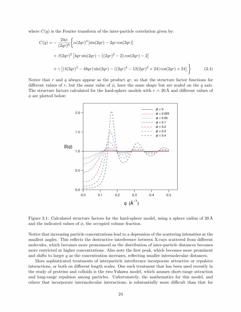
Notice that r and q always appear as the product qr, so that the structure factor functions fordifferent values of r, but the same value of φ, have the same shape but are scaled on the q axis.The structure factors calculated for the hard-sphere models with r = 20 A and different values ofφ are plotted below:
Figure 3.1: Calculated structure factors for the hard-sphere model, using a sphere radius of 20 Aand the indicated values of φ, the occupied volume fraction.
Notice that increasing particle concentrations lead to a depression of the scattering intensities at thesmallest angles. This reflects the destructive interference between X-rays scattered from differentmolecules, which becomes more pronounced as the distribution of inter-particle distances becomesmore restricted at higher concentrations. Also note the first peak, which becomes more prominentand shifts to larger q as the concentration increases, reflecting smaller intermolecular distances.
More sophisticated treatments of interparticle interference incorporate attractive or repulsiveinteractions, or both on different length scales. One such treatment that has been used recently inthe study of proteins and colloids is the two-Yukawa model, which asumes short-range attractionand long-range repulsion among particles. Unfortunately, the mathematics for this model, andothers that incorporate intermolecular interactions, is substantially more difficult than that for
24
the hard-sphere model, necessitating the use of numerical solutions or Monte Carlo simulations.The structure factor functions calculated for the two-Yukawa model is qualitatively similar to thatfor the hard-sphere model, with the notable addition of a peak at lower q-values reflecting theshort-range attraction between molecules.
Because the form factor (P (q)) and the structure factor (S(q)) are combined by a simple mul-tiplication to generate the observed intensities, I(q), their contributions can, in principle, be sep-arated from the experimental data. If either S(q) or P (q) is known (or hypothesized), the othercan be calculated by dividing the experimental intensities by the known function. Alternatively,model functions with adjustable parameters can be multiplied and used to fit the experimental datadirectly. It should be noted, however, that the multiplication or division is only valid after anybackground subtraction or desmearing has been applied. The Utah SAXS Tools includes facilitatefor these calculations using the hard-sphere model.
3.1 References on interparticle interference and structure func-tions
• Percus, J, K. & Yevick, G. J. (1958). Analysis of classical statistical mechanics by means ofcollective coordinates. Phys. Rev., 110, 1–13.http://dx.doi.org/10.1103/PhysRev.110.1
• Ashcroft, N. W. & Lekner, J. (1966). Structure and resistivity of liquid metals. Phys. Rev.,145, 83–90.http://dx.doi.org/10.1103/PhysRev.145.83
(Original solution of the structure factor for a hard-sphere fluid)
• Ailawadi, N. K. (1973). Possible generalization of the Ashcroft-Lekner hard-sphere model forthe structure factor. Phys. Rev. A, 7, 2200–2203.http://dx.doi.org/10.1103/PhysRevA.7.2200
(Includes explicit equations for the Ashcroft-Lekner solution, as used here)
• Hubbard, S. R. & Doniach, S. (1988). A Monte Carlo calculation of the interparticle inter-ference in small-angle X-ray scattering. J. Appl. Cryst., 21, 953–959.http://dx.doi.org/10.1107/S002188988800826X
• Sjoberg, B. (1999). Small-angle scattering from collections of interacting hard ellipsoids ofrevolution studied by Monte Carlo simulations and other methods of statistical analysis. J.Appl. Cryst., 32, 917–923.http://dx.doi.org/10.1107/S0021889899006640
• Shukla, A., Mylonas, E., Di Cola, E., Finet, S., Timmins, P., Narayanan, T. & Svergun, D. I.(2008). Absence of equilibrium cluster phase in concentrated lysozyme solutions. Proc. Natl.Acad. Sci., USA, 105, 5075–5078.http://dx.doi.org/10.1073/pnas.0711928105
• Broccio, M., Costa, D., Liu, Y. & Chen, S.-H. (2006). The structural properties of a two-Yukawa fluid: Simulation and analytical results. J. Chem. Phys., 124, 084501.http://link.aip.org/link/doi/10.1063/1.2166390
25
Chapter 4The Utah SAXS Tools
I have written a collection of small computer programs that, together, provide many of the necessarytools for processing and analyzing small-angle scattering data, with a particular focus on handlingthe smearing effects that arise when using a slit-collimated camera. For the present, these are calledthe Utah SAXS Tools (USToo). These tools were written for use with the data generated usingthe Anton Paar SAXSess instrument, and they offer much of the functionality of the proprietarySAXSquant software, though with a rather different user interface. Though they were written andhave only been tested using the Macintosh OS X operating system, they are based on open-sourcecross-platform programs, and there should be little difficulty in using them with other computers.
There are two major components of USToo. The first is a set of macros (saxsImage) for theimageJ program, a widely-used scientific image analysis program developed by Wayne Rasbandat the U.S. National Institutes of Health. The saxsImage macros create new menu commandsfor imageJ that are specifically designed for integrating the two-dimensional image data from theSAXSess camera, as well as analyzing the beam profile. The data from saxsImage are saved in thePDH file format of Glatter et al., with special provisions for storing the beam-profile information.
The second component of USToo is a set of programs, written in the Python language, forprocessing, analyzing and plotting the scattering data. These programs are run using a command-line interface: A shell in Unix-like operating systems (including Mac OS X) or the DOS window inWindows”. While this approach is, in some respects, less user-friendly than a graphical interfacewith menus etc., with a bit of experience it can become a very efficient way of working.
4.1 File Formats
The USToo programs use the PDH (Primary Data Handling) file format for scattering data, withsome the ”free” data fields used to handle the special information associated with the smearingeffects. The PDH format is the native format for the PCG (Physical Chemistry Graz) SAXSsoftware developed at the University of Graz by Prof. Otto Glatter and colleagues. The format isspecified in Appendix 8.1 of the PCG manual (page 123 in the 2005 edition).
A PDH file contains SAXS (or SANS) data in a simple three-column text format, with thecolumns containing the scattering vector magnitude (q), the scattering intensity (I) and the uncer-tainty in the intensity. The data columns are preceded by five lines of header information:
1. An experiment title or description of the experiment. Fortran format: A80
2. Keywords describing the experiment, read in groups of four characters separated by singlespaces. Fortran format: 16(A4,1X).
3. 8 integer constants. Fortran format: 8(I9,1X).
4. 5 floating point constants. Fortran format 5(E14.6,1X).
5. 5 floating point constants. Fortran format 5(E14.6,1X).
The subsequent data lines have fortran format 3(E14.6,1X). The Fortran formats very preciselyspecify the character positions of the fields, and also specify one blank character (1X) between thefields. When reading PDH files the USToo programs use the blank characters to parse the fields,
26
which allows some flexibility in the file format. But, this flexibility cannot be assumed for otherprograms, and the USToo programs use the stricter specification when writing files.
The specification for the PDH format sets aside two of the numerical constant fields for specificpurposes:
• The first integer constant in line 3 is the number of data points.
• The fourth floating-point constant in line 4 is a normalization factor, with a default value of1.0. It must not be 0.0 for the PCG programs.
The other constants in lines 3–5 can be used for special purposes by different programs. TheSAXSess software (SAXSquant) sets aside the following floating-point fields in line 4:
• Field 2: The sample-to-detector distance, in mm.
• Field 5: The X-ray wavelength.
Other fields may also be set aside by SAXSquant and other software.In addition to the fields identified above, the USToo programs use several of the header fields,
as follows:
• Field 2 in line 3: An integer specifying the function used to describe the beam-length profile:0: None. This usually indicates that there is no smearing, and the other smearing parametersare ignored.1: The sigmoidal function. (See page 6.)2: The trapezoidal function. (See page 5.)
• Field 3 in line 3: A flag to indicate that the data have been calibrated to absolute intensityin units of cm−1. Set to 1 if the data are calibrated, 0 otherwise.
• Field 1 in line 5: Beam-length profile parameter a.
• Field 2 in line 5: Beam-length profile parameter b.
• Field 3 in line 5: Half-width of the beam-width profile (at half height), in q-units.
• Field 4 in line 5: Detector-slit length (width of integration area), in q-units.
• Field 5 in line 5: Scale for units of q: 1 for A−1
, 10 for nm−1.
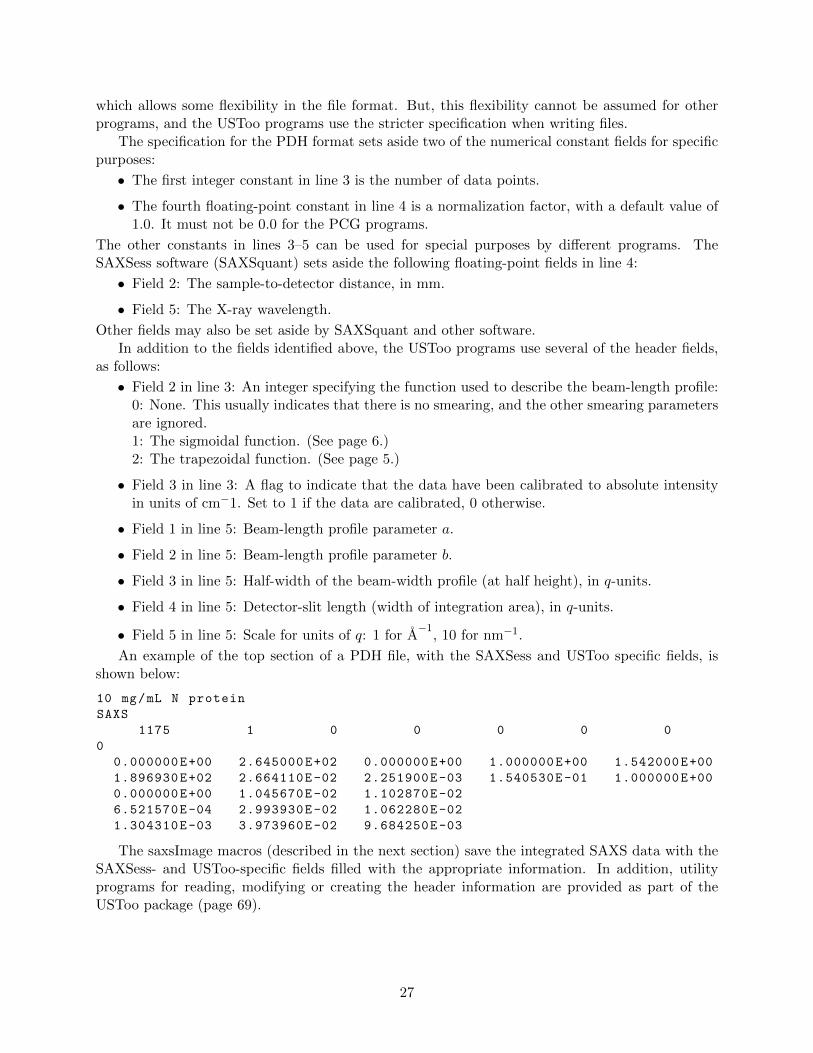
An example of the top section of a PDH file, with the SAXSess and USToo specific fields, isshown below:
10 mg/mL N protein
SAXS
1175 1 0 0 0 0 0
0
0.000000E+00 2.645000E+02 0.000000E+00 1.000000E+00 1.542000E+00
1.896930E+02 2.664110E-02 2.251900E-03 1.540530E-01 1.000000E+00
0.000000E+00 1.045670E-02 1.102870E-02
6.521570E-04 2.993930E-02 1.062280E-02
1.304310E-03 3.973960E-02 9.684250E-03
The saxsImage macros (described in the next section) save the integrated SAXS data with theSAXSess- and USToo-specific fields filled with the appropriate information. In addition, utilityprograms for reading, modifying or creating the header information are provided as part of theUSToo package (page 69).
27
4.2 saxsImage macros for ImageJ
ImageJ is a very powerful and free image processing program written by Wayne Rasband of theU.S. NIH. ImageJ is a successor to NIH Image (which was written for the Macintosh) and is writtenin Java, making it compatible with any operating system with a Java runtime environment. Theprogram can be enhanced with the addition of custom scripts, macros or plugins; which differsomewhat in their structures and capabilities. The tools provided here are classed as macros, andwere written using the ImageJ-specific macro language.ImageJ can be obtained from: http://rsbweb.nih.gov/ij/ The program is frequently updatedwith new features and bug fixes, but is in some regards a victim of its own success, as the updatesfrequently introduce bugs or conflicts with plugins or macros. As of April 2012, the saxsImagemacros appear to work well with ImageJ versions through 1.44o, but I have encountered problemswith versions 1.45 and 1.46. Fortunately, older versions remain available at http://imagej.nih.
gov/ij/download/. A major update of ImageJ (ImageJ 2) is currently being developed as anorganized open-source project, as described at: http://developer.imagej.net/, and the firstbeta-version was released in April 2012. The beta does not support the saxsImage macros, butfuture versions may well, since compatibility with ImageJ 1.x macros is a major goal of the project.
4.2.1 Installing and opening the macros
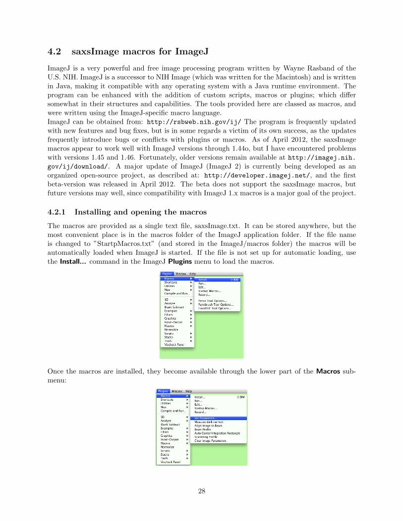
The macros are provided as a single text file, saxsImage.txt. It can be stored anywhere, but themost convenient place is in the macros folder of the ImageJ application folder. If the file nameis changed to ”StartpMacros.txt” (and stored in the ImageJ/macros folder) the macros will beautomatically loaded when ImageJ is started. If the file is not set up for automatic loading, usethe Install... command in the ImageJ Plugins menu to load the macros.
Once the macros are installed, they become available through the lower part of the Macros sub-menu:
28
The individual macro commands are listed in the order in which they are normally used in processinga SAXS image, as described on the following pages.
4.2.2 Macro commands
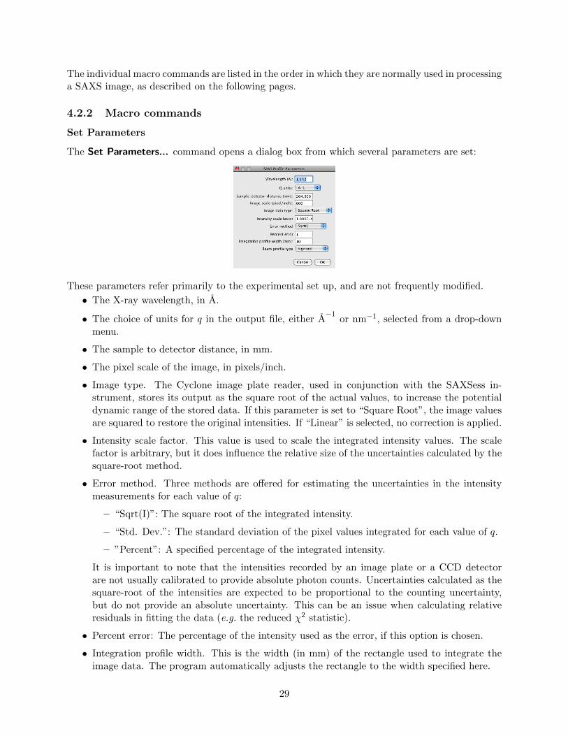
Set Parameters
The Set Parameters... command opens a dialog box from which several parameters are set:
These parameters refer primarily to the experimental set up, and are not frequently modified.
• The X-ray wavelength, in A.
• The choice of units for q in the output file, either A−1
or nm−1, selected from a drop-downmenu.
• The sample to detector distance, in mm.
• The pixel scale of the image, in pixels/inch.
• Image type. The Cyclone image plate reader, used in conjunction with the SAXSess in-strument, stores its output as the square root of the actual values, to increase the potentialdynamic range of the stored data. If this parameter is set to “Square Root”, the image valuesare squared to restore the original intensities. If “Linear” is selected, no correction is applied.
• Intensity scale factor. This value is used to scale the integrated intensity values. The scalefactor is arbitrary, but it does influence the relative size of the uncertainties calculated by thesquare-root method.
• Error method. Three methods are offered for estimating the uncertainties in the intensitymeasurements for each value of q:
– “Sqrt(I)”: The square root of the integrated intensity.
– “Std. Dev.”: The standard deviation of the pixel values integrated for each value of q.
– ”Percent”: A specified percentage of the integrated intensity.
It is important to note that the intensities recorded by an image plate or a CCD detectorare not usually calibrated to provide absolute photon counts. Uncertainties calculated as thesquare-root of the intensities are expected to be proportional to the counting uncertainty,but do not provide an absolute uncertainty. This can be an issue when calculating relativeresiduals in fitting the data (e.g. the reduced χ2 statistic).
• Percent error: The percentage of the intensity used as the error, if this option is chosen.
• Integration profile width. This is the width (in mm) of the rectangle used to integrate theimage data. The program automatically adjusts the rectangle to the width specified here.
29
• Beam profile type: The mathematical function used to represent the beam profile in theoutput file, either “Sigmoid” or “Trapezoid”, selected from a drop-down menu.
Once set, these parameters will be used for all of the macros during a session, but they will notbe saved when ImageJ is closed. The macro file can be edited, using a text editor, to change thedefault values of the parameters. The relevant lines are found near the top of the file:
var wavelength =1.542; // X-ray wavelength
var qUnits="A-1"; // qUnits - either "A-1" or "nm -1"
var sdDistance =264.5; // sample -detector distance , in mm
var imageScale =600; // pixels per inch
var imageDataType="Square Root"; // "Linear" or "Square Root"
var iScale =1E-4; // scaling factor for intensities
var errMethod="Sqrt(I)"; // method for errors , "Sqrt(I)","Std. Dev." or "Percent I"
var errPerc =1.0; // value for calculating error by percent method
var profWidth =10; // width of profile for integration , in mm
var beamProfType = "Sigmoid"; // beam profile type: "Sigmoid" or "Trapezoid"
After editing this file, it must be saved and read back into ImageJ, using the Install... commandin the Plugins menu.
Measure Dark Current
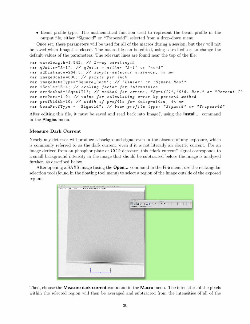
Nearly any detector will produce a background signal even in the absence of any exposure, whichis commonly referred to as the dark current, even if it is not literally an electric current. For animage derived from an phosphor plate or CCD detector, this “dark current” signal corresponds toa small background intensity in the image that should be subtracted before the image is analyzedfurther, as described below.
After opening a SAXS image (using the Open... command in the File menu, use the rectangularselection tool (found in the floating tool menu) to select a region of the image outside of the exposedregion:
Then, choose the Measure dark current command in the Macro menu. The intensities of the pixelswithin the selected region will then be averaged and subtracted from the intensities of all of the
30

image pixels.
Align Image to Beam
In order to accurately integrate the SAXS data, a rectangular region perpendicular to the beamprofile must be selected. Often, the camera image is not quite aligned squarely with the surroundingimage, as shown below:
To correct the alignment, first select a rectangular region around the central part of the beam,making the selection as narrow as possible, as in the figure above. Then, choose the Align Imageto Beam command in the Macro menu. The program will identify the peak positions in the beamprofile, determine the slope of the beam and rotate the image to make the beam horizontal:
31
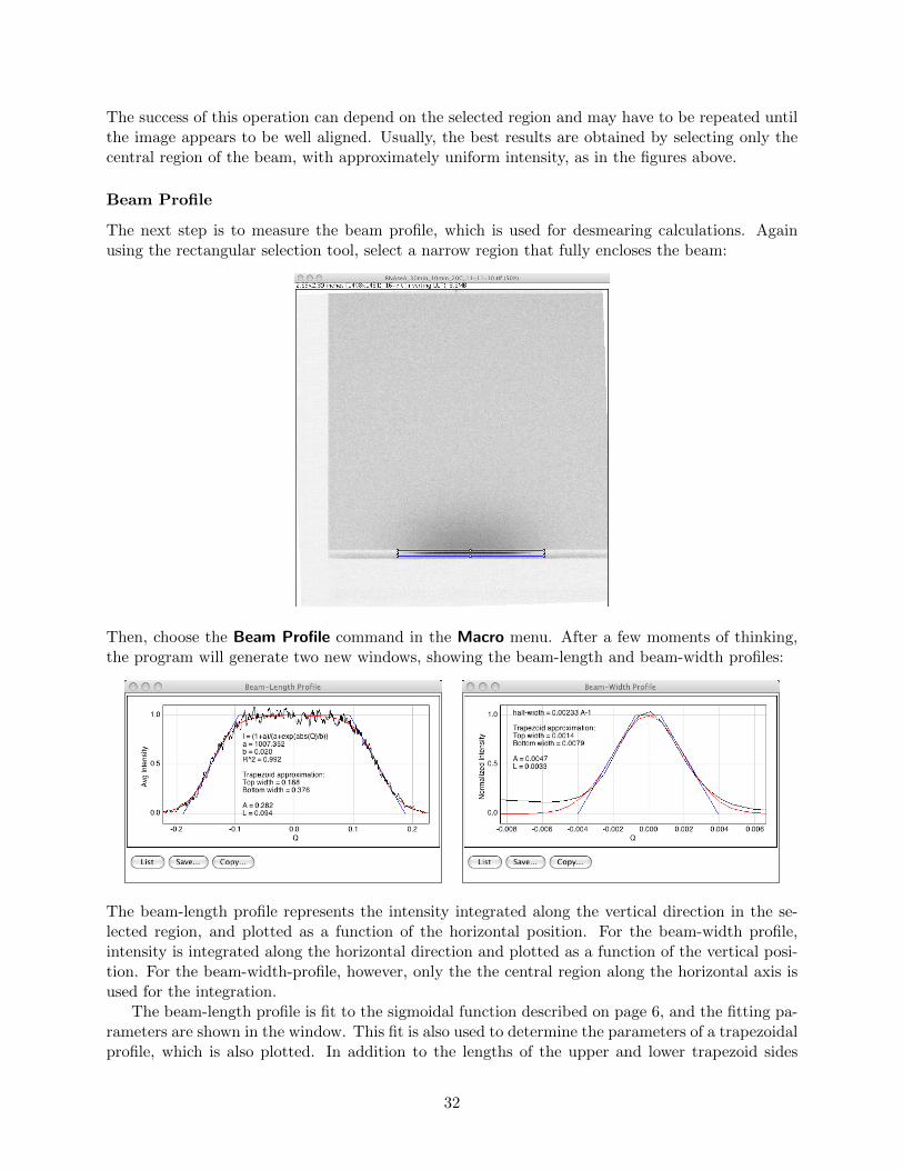
The success of this operation can depend on the selected region and may have to be repeated untilthe image appears to be well aligned. Usually, the best results are obtained by selecting only thecentral region of the beam, with approximately uniform intensity, as in the figures above.
Beam Profile
The next step is to measure the beam profile, which is used for desmearing calculations. Againusing the rectangular selection tool, select a narrow region that fully encloses the beam:
Then, choose the Beam Profile command in the Macro menu. After a few moments of thinking,the program will generate two new windows, showing the beam-length and beam-width profiles:
The beam-length profile represents the intensity integrated along the vertical direction in the se-lected region, and plotted as a function of the horizontal position. For the beam-width profile,intensity is integrated along the horizontal direction and plotted as a function of the vertical posi-tion. For the beam-width-profile, however, only the the central region along the horizontal axis isused for the integration.
The beam-length profile is fit to the sigmoidal function described on page 6, and the fitting pa-rameters are shown in the window. This fit is also used to determine the parameters of a trapezoidalprofile, which is also plotted. In addition to the lengths of the upper and lower trapezoid sides
32
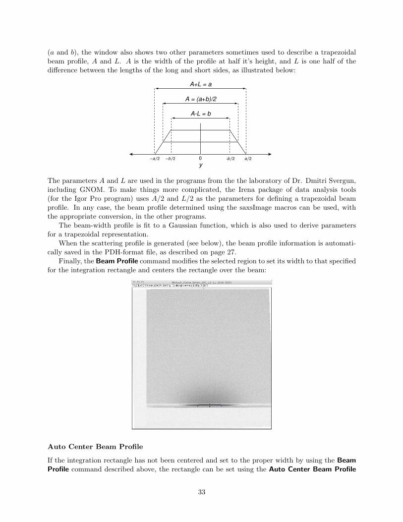
(a and b), the window also shows two other parameters sometimes used to describe a trapezoidalbeam profile, A and L. A is the width of the profile at half it’s height, and L is one half of thedifference between the lengths of the long and short sides, as illustrated below:
0
A = (a+b)/2
A+L = a
A-L = b
The parameters A and L are used in the programs from the the laboratory of Dr. Dmitri Svergun,including GNOM. To make things more complicated, the Irena package of data analysis tools(for the Igor Pro program) uses A/2 and L/2 as the parameters for defining a trapezoidal beamprofile. In any case, the beam profile determined using the saxsImage macros can be used, withthe appropriate conversion, in the other programs.
The beam-width profile is fit to a Gaussian function, which is also used to derive parametersfor a trapezoidal representation.
When the scattering profile is generated (see below), the beam profile information is automati-cally saved in the PDH-format file, as described on page 27.
Finally, the Beam Profile command modifies the selected region to set its width to that specifiedfor the integration rectangle and centers the rectangle over the beam:
Auto Center Beam Profile
If the integration rectangle has not been centered and set to the proper width by using the BeamProfile command described above, the rectangle can be set using the Auto Center Beam Profile
33
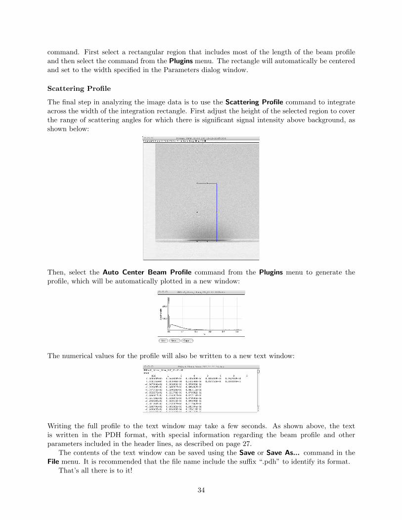
command. First select a rectangular region that includes most of the length of the beam profileand then select the command from the Plugins menu. The rectangle will automatically be centeredand set to the width specified in the Parameters dialog window.
Scattering Profile
The final step in analyzing the image data is to use the Scattering Profile command to integrateacross the width of the integration rectangle. First adjust the height of the selected region to coverthe range of scattering angles for which there is significant signal intensity above background, asshown below:
Then, select the Auto Center Beam Profile command from the Plugins menu to generate theprofile, which will be automatically plotted in a new window:
The numerical values for the profile will also be written to a new text window:
Writing the full profile to the text window may take a few seconds. As shown above, the textis written in the PDH format, with special information regarding the beam profile and otherparameters included in the header lines, as described on page 27.
The contents of the text window can be saved using the Save or Save As... command in theFile menu. It is recommended that the file name include the suffix “.pdh” to identify its format.
That’s all there is to it!
34
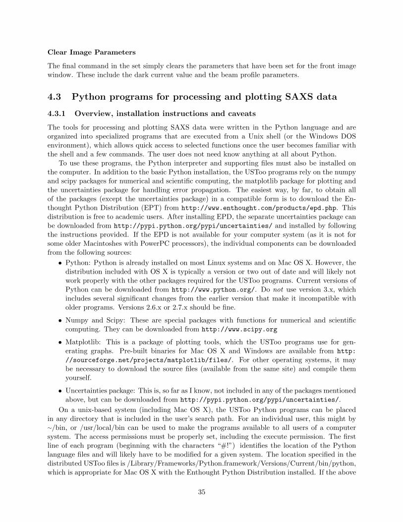
Clear Image Parameters
The final command in the set simply clears the parameters that have been set for the front imagewindow. These include the dark current value and the beam profile parameters.
4.3 Python programs for processing and plotting SAXS data
4.3.1 Overview, installation instructions and caveats
The tools for processing and plotting SAXS data were written in the Python language and areorganized into specialized programs that are executed from a Unix shell (or the Windows DOSenvironment), which allows quick access to selected functions once the user becomes familiar withthe shell and a few commands. The user does not need know anything at all about Python.
To use these programs, the Python interpreter and supporting files must also be installed onthe computer. In addition to the basic Python installation, the USToo programs rely on the numpyand scipy packages for numerical and scientific computing, the matplotlib package for plotting andthe uncertainties package for handling error propagation. The easiest way, by far, to obtain allof the packages (except the uncertainties package) in a compatible form is to download the En-thought Python Distribution (EPT) from http://www.enthought.com/products/epd.php. Thisdistribution is free to academic users. After installing EPD, the separate uncertainties package canbe downloaded from http://pypi.python.org/pypi/uncertainties/ and installed by followingthe instructions provided. If the EPD is not available for your computer system (as it is not forsome older Macintoshes with PowerPC processors), the individual components can be downloadedfrom the following sources:
• Python: Python is already installed on most Linux systems and on Mac OS X. However, thedistribution included with OS X is typically a version or two out of date and will likely notwork properly with the other packages required for the USToo programs. Current versions ofPython can be downloaded from http://www.python.org/. Do not use version 3.x, whichincludes several significant changes from the earlier version that make it incompatible witholder programs. Versions 2.6.x or 2.7.x should be fine.
• Numpy and Scipy: These are special packages with functions for numerical and scientificcomputing. They can be downloaded from http://www.scipy.org
• Matplotlib: This is a package of plotting tools, which the USToo programs use for gen-erating graphs. Pre-built binaries for Mac OS X and Windows are available from http:
//sourceforge.net/projects/matplotlib/files/. For other operating systems, it maybe necessary to download the source files (available from the same site) and compile themyourself.
• Uncertainties package: This is, so far as I know, not included in any of the packages mentionedabove, but can be downloaded from http://pypi.python.org/pypi/uncertainties/.
On a unix-based system (including Mac OS X), the USToo Python programs can be placedin any directory that is included in the user’s search path. For an individual user, this might by∼/bin, or /usr/local/bin can be used to make the programs available to all users of a computersystem. The access permissions must be properly set, including the execute permission. The firstline of each program (beginning with the characters “#!”) identifies the location of the Pythonlanguage files and will likely have to be modified for a given system. The location specified in thedistributed USToo files is /Library/Frameworks/Python.framework/Versions/Current/bin/python,which is appropriate for Mac OS X with the Enthought Python Distribution installed. If the above
35
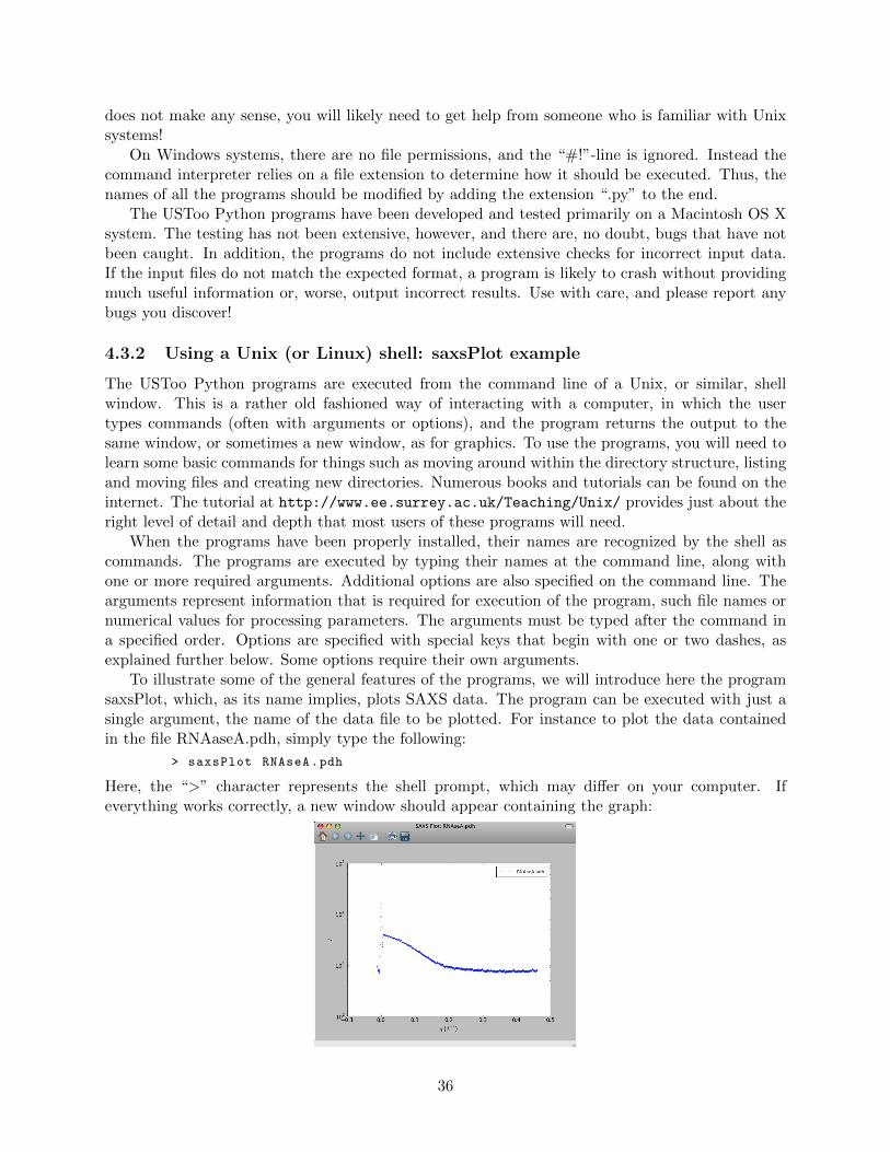
does not make any sense, you will likely need to get help from someone who is familiar with Unixsystems!
On Windows systems, there are no file permissions, and the “#!”-line is ignored. Instead thecommand interpreter relies on a file extension to determine how it should be executed. Thus, thenames of all the programs should be modified by adding the extension “.py” to the end.
The USToo Python programs have been developed and tested primarily on a Macintosh OS Xsystem. The testing has not been extensive, however, and there are, no doubt, bugs that have notbeen caught. In addition, the programs do not include extensive checks for incorrect input data.If the input files do not match the expected format, a program is likely to crash without providingmuch useful information or, worse, output incorrect results. Use with care, and please report anybugs you discover!
4.3.2 Using a Unix (or Linux) shell: saxsPlot example
The USToo Python programs are executed from the command line of a Unix, or similar, shellwindow. This is a rather old fashioned way of interacting with a computer, in which the usertypes commands (often with arguments or options), and the program returns the output to thesame window, or sometimes a new window, as for graphics. To use the programs, you will need tolearn some basic commands for things such as moving around within the directory structure, listingand moving files and creating new directories. Numerous books and tutorials can be found on theinternet. The tutorial at http://www.ee.surrey.ac.uk/Teaching/Unix/ provides just about theright level of detail and depth that most users of these programs will need.
When the programs have been properly installed, their names are recognized by the shell ascommands. The programs are executed by typing their names at the command line, along withone or more required arguments. Additional options are also specified on the command line. Thearguments represent information that is required for execution of the program, such file names ornumerical values for processing parameters. The arguments must be typed after the command ina specified order. Options are specified with special keys that begin with one or two dashes, asexplained further below. Some options require their own arguments.
To illustrate some of the general features of the programs, we will introduce here the programsaxsPlot, which, as its name implies, plots SAXS data. The program can be executed with just asingle argument, the name of the data file to be plotted. For instance to plot the data containedin the file RNAaseA.pdh, simply type the following:
> saxsPlot RNAseA.pdh
Here, the “>” character represents the shell prompt, which may differ on your computer. Ifeverything works correctly, a new window should appear containing the graph:
36
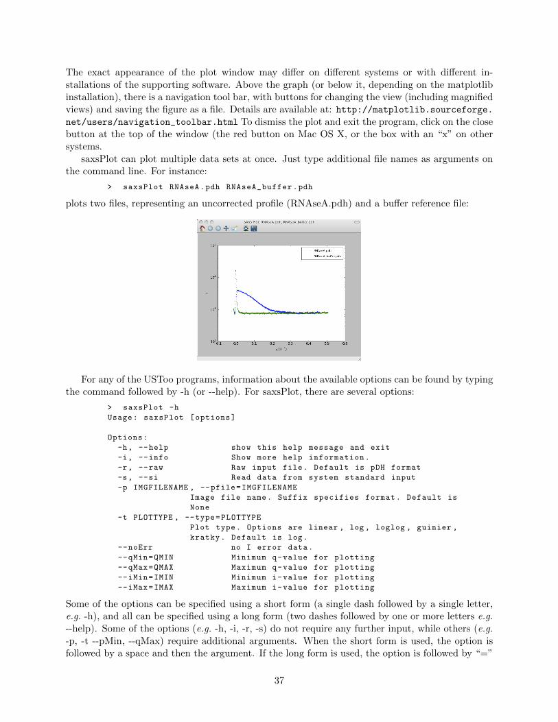
The exact appearance of the plot window may differ on different systems or with different in-stallations of the supporting software. Above the graph (or below it, depending on the matplotlibinstallation), there is a navigation tool bar, with buttons for changing the view (including magnifiedviews) and saving the figure as a file. Details are available at: http://matplotlib.sourceforge.net/users/navigation_toolbar.html To dismiss the plot and exit the program, click on the closebutton at the top of the window (the red button on Mac OS X, or the box with an “x” on othersystems.
saxsPlot can plot multiple data sets at once. Just type additional file names as arguments onthe command line. For instance:
> saxsPlot RNAseA.pdh RNAseA_buffer.pdh
plots two files, representing an uncorrected profile (RNAseA.pdh) and a buffer reference file:
For any of the USToo programs, information about the available options can be found by typingthe command followed by -h (or --help). For saxsPlot, there are several options:
> saxsPlot -h
Usage: saxsPlot [options]
Options:
-h, --help show this help message and exit
-i, --info Show more help information.
-r, --raw Raw input file. Default is pDH format
-s, --si Read data from system standard input
-p IMGFILENAME , --pfile=IMGFILENAME
Image file name. Suffix specifies format. Default is
None
-t PLOTTYPE , --type=PLOTTYPE
Plot type. Options are linear , log , loglog , guinier ,
kratky. Default is log.
--noErr no I error data.
--qMin=QMIN Minimum q-value for plotting
--qMax=QMAX Maximum q-value for plotting
--iMin=IMIN Minimum i-value for plotting
--iMax=IMAX Maximum i-value for plotting
Some of the options can be specified using a short form (a single dash followed by a single letter,e.g. -h), and all can be specified using a long form (two dashes followed by one or more letters e.g.--help). Some of the options (e.g. -h, -i, -r, -s) do not require any further input, while others (e.g.-p, -t --pMin, --qMax) require additional arguments. When the short form is used, the option isfollowed by a space and then the argument. If the long form is used, the option is followed by “=”
37

and the argument.
The various options, many of which are shared other programs in USToo are described below.
• -h or --help. Prints the help message with all of the available options and exits the program.
• -i or --info. Prints a more extensive information message and exits the program.
• -r or --raw. By default, the program expects a SAXS data file in the pDH format, as describedon page 26. If the -r or --raw option is used, the program accepts a file with a simple threecolumn format, with the columns containing values for q, I and the errors associated with I.If the --noErr option is also used, only two columns are required.
• -s or --si. This option causes the program to read a single data file from standard input,explained further below. With this option, no file names are read as arguments, and thecommand is executed as:
> saxsPlot < inputFileName
The “<” indicates that the file is to be read as standard input. For more about file direction,see http://www.ee.surrey.ac.uk/Teaching/Unix/unix3.html.
• -p or --pfile. This allows the user to specify the name of a file in which to save an image ofthe plot. This is an example of an option that requires an argument. It’s use looks like this:
> saxsPlot -p myPlot.pdf RNAseA.pdh
or
> saxsPlot --pfile=myPlot.pdf RNAseA.pdh
The extension of the file name specifies the image format. If no extension is used, the defaultformat is png. Other options are: emf, eps, pdf, ps, raw, rgba, svg, svgz. An image file canalso be saved from the plot window by clicking the disk icon, which brings up a save-file dialogwindow. Again, the format of the image file is specified by the file name extension.
• -t --type. By default, the SAXS data are plotted as log I versus q. Other options are: a linearplot of I versus q (‘linear’), a plot of log I versus log q (’loglog’), a Guinier plot of ln I versusq2 (‘guinier’) and a Kratky plot of Iq2 versus q (kratky). For instance, to make a Guinierplot, type:
> saxsPlot -t Guinier RNAseA.pdh
or
saxsPlot --type=Guinier RNAseA.pdh
• --noErr. By default the program plots the values of I as single points with error error bars.With the --noErr option, no error bars are shown and the individual data points are joinedwith line segments. To plot data sets that do not contain error bars, use the --noErr and--raw options together.
• --qMin and --qMax. These options can be used separately or together and allow the user tospecify the range of q-values included in the plot.
• --iMin and --iMax. These options can be used separately or together and allow the user tospecify the range of I-values included in the plot.
The options can be used in combination to customize the plot, as shown in the example below:
38
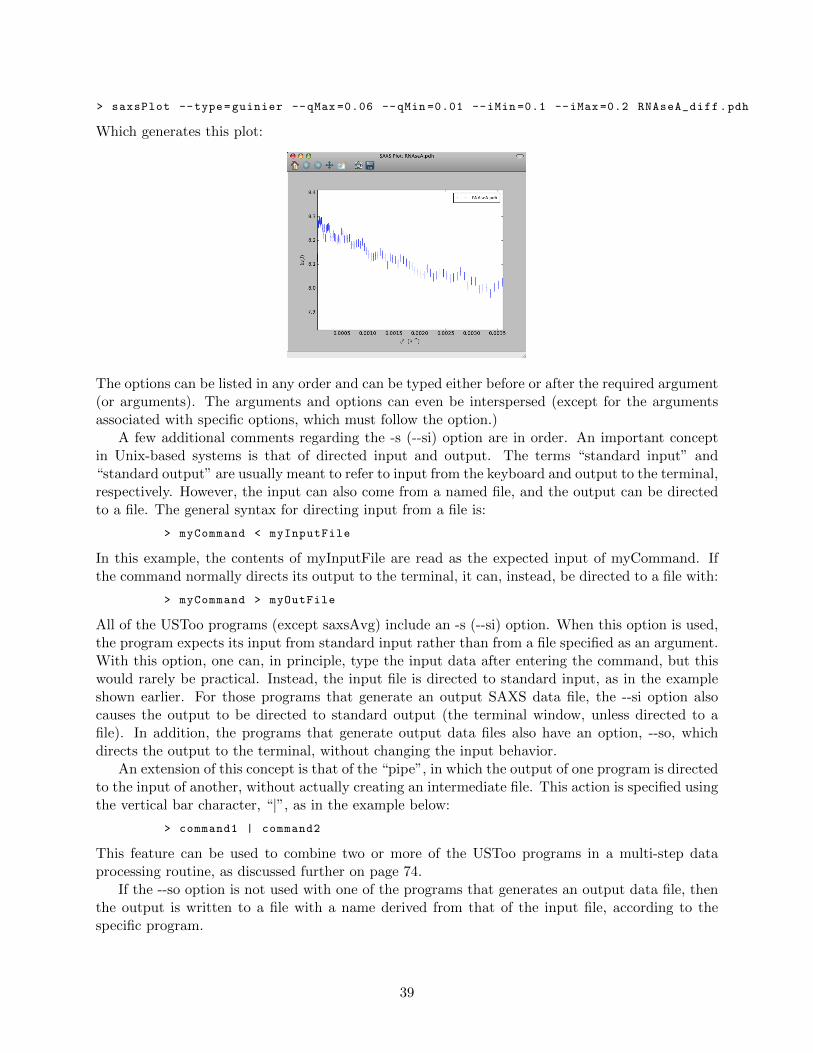
> saxsPlot --type=guinier --qMax =0.06 --qMin =0.01 --iMin =0.1 --iMax =0.2 RNAseA_diff.pdh
Which generates this plot:
The options can be listed in any order and can be typed either before or after the required argument(or arguments). The arguments and options can even be interspersed (except for the argumentsassociated with specific options, which must follow the option.)
A few additional comments regarding the -s (--si) option are in order. An important conceptin Unix-based systems is that of directed input and output. The terms “standard input” and“standard output” are usually meant to refer to input from the keyboard and output to the terminal,respectively. However, the input can also come from a named file, and the output can be directedto a file. The general syntax for directing input from a file is:
> myCommand < myInputFile
In this example, the contents of myInputFile are read as the expected input of myCommand. Ifthe command normally directs its output to the terminal, it can, instead, be directed to a file with:
> myCommand > myOutFile
All of the USToo programs (except saxsAvg) include an -s (--si) option. When this option is used,the program expects its input from standard input rather than from a file specified as an argument.With this option, one can, in principle, type the input data after entering the command, but thiswould rarely be practical. Instead, the input file is directed to standard input, as in the exampleshown earlier. For those programs that generate an output SAXS data file, the --si option alsocauses the output to be directed to standard output (the terminal window, unless directed to afile). In addition, the programs that generate output data files also have an option, --so, whichdirects the output to the terminal, without changing the input behavior.
An extension of this concept is that of the “pipe”, in which the output of one program is directedto the input of another, without actually creating an intermediate file. This action is specified usingthe vertical bar character, “|”, as in the example below:
> command1 | command2
This feature can be used to combine two or more of the USToo programs in a multi-step dataprocessing routine, as discussed further on page 74.
If the --so option is not used with one of the programs that generates an output data file, thenthe output is written to a file with a name derived from that of the input file, according to thespecific program.
39
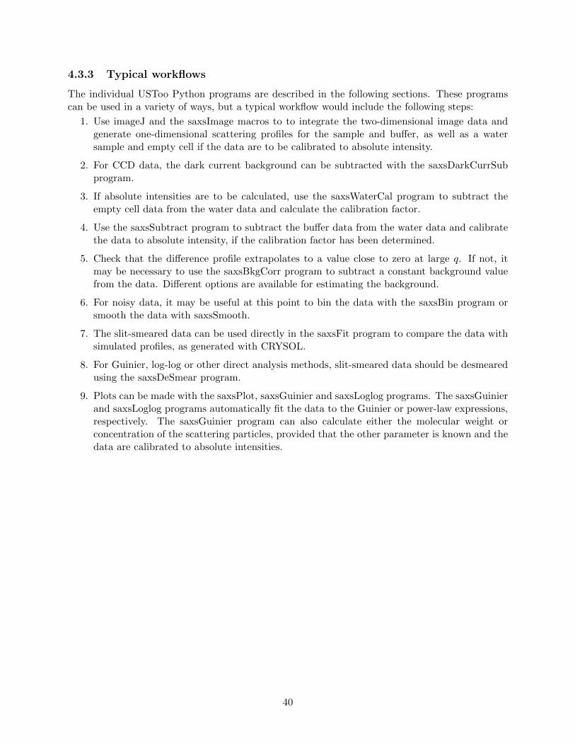
4.3.3 Typical workflows
The individual USToo Python programs are described in the following sections. These programscan be used in a variety of ways, but a typical workflow would include the following steps:
1. Use imageJ and the saxsImage macros to to integrate the two-dimensional image data andgenerate one-dimensional scattering profiles for the sample and buffer, as well as a watersample and empty cell if the data are to be calibrated to absolute intensity.
2. For CCD data, the dark current background can be subtracted with the saxsDarkCurrSubprogram.
3. If absolute intensities are to be calculated, use the saxsWaterCal program to subtract theempty cell data from the water data and calculate the calibration factor.
4. Use the saxsSubtract program to subtract the buffer data from the water data and calibratethe data to absolute intensity, if the calibration factor has been determined.
5. Check that the difference profile extrapolates to a value close to zero at large q. If not, itmay be necessary to use the saxsBkgCorr program to subtract a constant background valuefrom the data. Different options are available for estimating the background.
6. For noisy data, it may be useful at this point to bin the data with the saxsBin program orsmooth the data with saxsSmooth.
7. The slit-smeared data can be used directly in the saxsFit program to compare the data withsimulated profiles, as generated with CRYSOL.
8. For Guinier, log-log or other direct analysis methods, slit-smeared data should be desmearedusing the saxsDeSmear program.
9. Plots can be made with the saxsPlot, saxsGuinier and saxsLoglog programs. The saxsGuinierand saxsLoglog programs automatically fit the data to the Guinier or power-law expressions,respectively. The saxsGuinier program can also calculate either the molecular weight orconcentration of the scattering particles, provided that the other parameter is known and thedata are calibrated to absolute intensities.
40
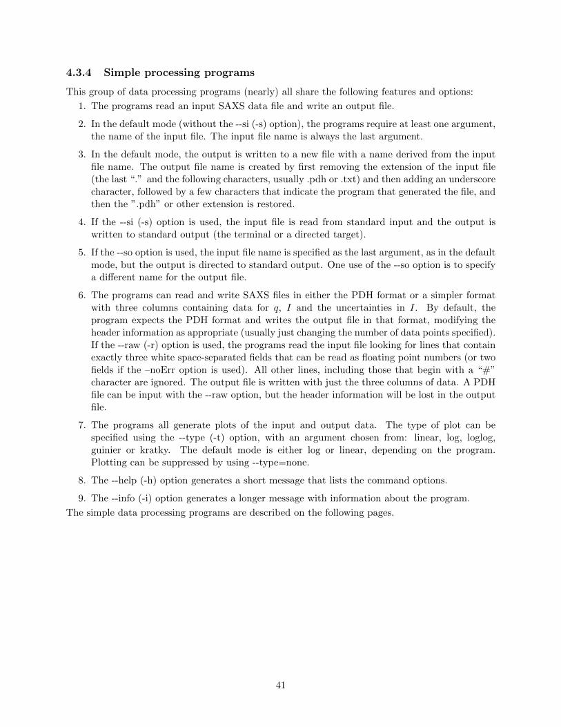
4.3.4 Simple processing programs
This group of data processing programs (nearly) all share the following features and options:
1. The programs read an input SAXS data file and write an output file.
2. In the default mode (without the --si (-s) option), the programs require at least one argument,the name of the input file. The input file name is always the last argument.
3. In the default mode, the output is written to a new file with a name derived from the inputfile name. The output file name is created by first removing the extension of the input file(the last “.” and the following characters, usually .pdh or .txt) and then adding an underscorecharacter, followed by a few characters that indicate the program that generated the file, andthen the ”.pdh” or other extension is restored.
4. If the --si (-s) option is used, the input file is read from standard input and the output iswritten to standard output (the terminal or a directed target).
5. If the --so option is used, the input file name is specified as the last argument, as in the defaultmode, but the output is directed to standard output. One use of the --so option is to specifya different name for the output file.
6. The programs can read and write SAXS files in either the PDH format or a simpler formatwith three columns containing data for q, I and the uncertainties in I. By default, theprogram expects the PDH format and writes the output file in that format, modifying theheader information as appropriate (usually just changing the number of data points specified).If the --raw (-r) option is used, the programs read the input file looking for lines that containexactly three white space-separated fields that can be read as floating point numbers (or twofields if the –noErr option is used). All other lines, including those that begin with a “#”character are ignored. The output file is written with just the three columns of data. A PDHfile can be input with the --raw option, but the header information will be lost in the outputfile.
7. The programs all generate plots of the input and output data. The type of plot can bespecified using the --type (-t) option, with an argument chosen from: linear, log, loglog,guinier or kratky. The default mode is either log or linear, depending on the program.Plotting can be suppressed by using --type=none.
8. The --help (-h) option generates a short message that lists the command options.
9. The --info (-i) option generates a longer message with information about the program.
The simple data processing programs are described on the following pages.
41
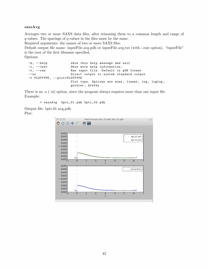
saxsAvg
Averages two or more SAXS data files, after trimming them to a common length and range ofq-values. The spacings of q-values in the files must be the same.Required arguments: the names of two or more SAXS files.Default output file name: inputFile avg.pdh or inputFile avg.txt (with --raw option). “inputFile”is the root of the first filename specified.Options:
-h, --help show this help message and exit
-i, --info Show more help information.
-r, --raw Raw input file. Default is pDH format
--so Direct output to system standard output
-t PLOTTYPE , --plot=PLOTTYPE
Plot type. Options are none , linear , log , loglog ,
guinier , kratky
There is no -s (–si) option, since the program always requires more than one input file.Example:
> saxsAvg bpti_01.pdh bpti_02.pdh
Output file: bpti 01 avg.pdhPlot:
42
saxsBinData
Bins (averages) sequential data points in a SAXS profile. Number of points to average is specifiedby the --nAvg or --dQ options. Default is to average 4 points. The --dQ option overrides --nAvg.Required argument: name of input file (or directed input with --si option)Default output file name: inputFile bin.pdh or inputFile bin.txt (with --raw option)Options:
-h, --help show this help message and exit
-i, --info Show more help information.
-r, --raw Raw input file. Default is pDH format
-s, --si Read data from system standard input and write to
standard output
--so Direct output to system standard output
-n NAVG , --nAvg=NAVG Number of points for averaging. Default is 4
-d DQ , --dQ=DQ Delta Q to determine averaging. Overrides nAvg.
-t PLOTTYPE , --plot=PLOTTYPE
Plot type. Options are none , linear , log , loglog ,
guinier , kratky. Default is linear
Example:
> saxsBinData --nAvg =10 RNAseA.pdh
Output file: RNAseA bin.pdhPlot:
43
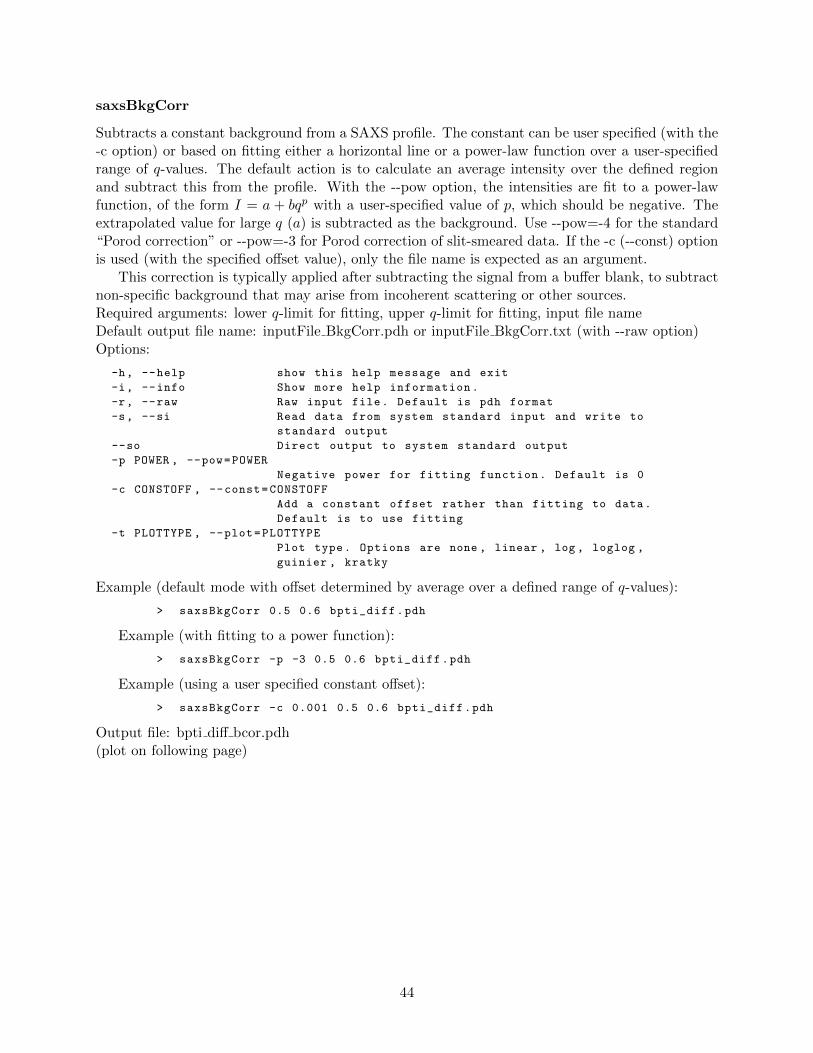
saxsBkgCorr
Subtracts a constant background from a SAXS profile. The constant can be user specified (with the-c option) or based on fitting either a horizontal line or a power-law function over a user-specifiedrange of q-values. The default action is to calculate an average intensity over the defined regionand subtract this from the profile. With the --pow option, the intensities are fit to a power-lawfunction, of the form I = a + bqp with a user-specified value of p, which should be negative. Theextrapolated value for large q (a) is subtracted as the background. Use --pow=-4 for the standard“Porod correction” or --pow=-3 for Porod correction of slit-smeared data. If the -c (--const) optionis used (with the specified offset value), only the file name is expected as an argument.
This correction is typically applied after subtracting the signal from a buffer blank, to subtractnon-specific background that may arise from incoherent scattering or other sources.Required arguments: lower q-limit for fitting, upper q-limit for fitting, input file nameDefault output file name: inputFile BkgCorr.pdh or inputFile BkgCorr.txt (with --raw option)Options:
-h, --help show this help message and exit
-i, --info Show more help information.
-r, --raw Raw input file. Default is pdh format
-s, --si Read data from system standard input and write to
standard output
--so Direct output to system standard output
-p POWER , --pow=POWER
Negative power for fitting function. Default is 0
-c CONSTOFF , --const=CONSTOFF
Add a constant offset rather than fitting to data.
Default is to use fitting
-t PLOTTYPE , --plot=PLOTTYPE
Plot type. Options are none , linear , log , loglog ,
guinier , kratky
Example (default mode with offset determined by average over a defined range of q-values):
> saxsBkgCorr 0.5 0.6 bpti_diff.pdh
Example (with fitting to a power function):
> saxsBkgCorr -p -3 0.5 0.6 bpti_diff.pdh
Example (using a user specified constant offset):
> saxsBkgCorr -c 0.001 0.5 0.6 bpti_diff.pdh
Output file: bpti diff bcor.pdh(plot on following page)
44
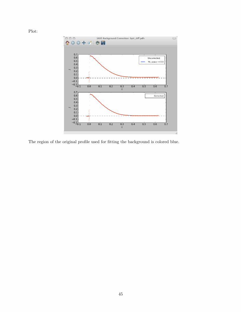
Plot:
The region of the original profile used for fitting the background is colored blue.
45
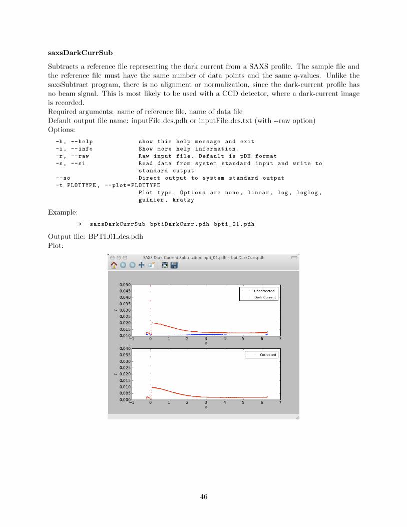
saxsDarkCurrSub
Subtracts a reference file representing the dark current from a SAXS profile. The sample file andthe reference file must have the same number of data points and the same q-values. Unlike thesaxsSubtract program, there is no alignment or normalization, since the dark-current profile hasno beam signal. This is most likely to be used with a CCD detector, where a dark-current imageis recorded.Required arguments: name of reference file, name of data fileDefault output file name: inputFile dcs.pdh or inputFile dcs.txt (with --raw option)Options:
-h, --help show this help message and exit
-i, --info Show more help information.
-r, --raw Raw input file. Default is pDH format
-s, --si Read data from system standard input and write to
standard output
--so Direct output to system standard output
-t PLOTTYPE , --plot=PLOTTYPE
Plot type. Options are none , linear , log , loglog ,
guinier , kratky
Example:
> saxsDarkCurrSub bptiDarkCurr.pdh bpti_01.pdh
Output file: BPTI 01 dcs.pdhPlot:
46
saxsDiv
Divides one SAXS profile by another (the divisor file). This can be used to divide experimental databy model data representing a form or structure factor. The divisor file is assumed to be composedof just two columns, I and q. Lines in the divisor file that do not contain exactly two fields withfloating point numbers are ignored. A cubic spline is used to represent the divisor data, so that thetwo files are not required to match one another point for point. If the --scale option is used, thedivisor file is first divided by the scale factor. Note that dividing an experimental profile by a formfactor or structure factor function is only valid or point-collimated or desmeared line-collimateddata.Required arguments: name of file with divisor data, name of file with data to be dividedDefault output file name: inputFile div.pdh or inputFile div.txt (with --raw option)Options:
-h, --help show this help message and exit
-i, --info Show more help information.
-r, --raw Raw input file. Default is pdh format
--noErr no I error data.
--scale=SCALEFACT Divisor data is divided by scale factor. Default = 1.0
-s, --si Read data from system standard input and write to
standard output
--so Direct output to system standard output
-t PLOTTYPE , --plot=PLOTTYPE
Plot type. Options are none , linear , log , loglog ,
guinier , kratky. Default is linear
Example:
> saxsDiv --scale =5e6 1ymbCrysol.txt Mb_diff_bcor_dsm.pdh
Output file: Mb diff bcor dsm div.pdhPlot:
47
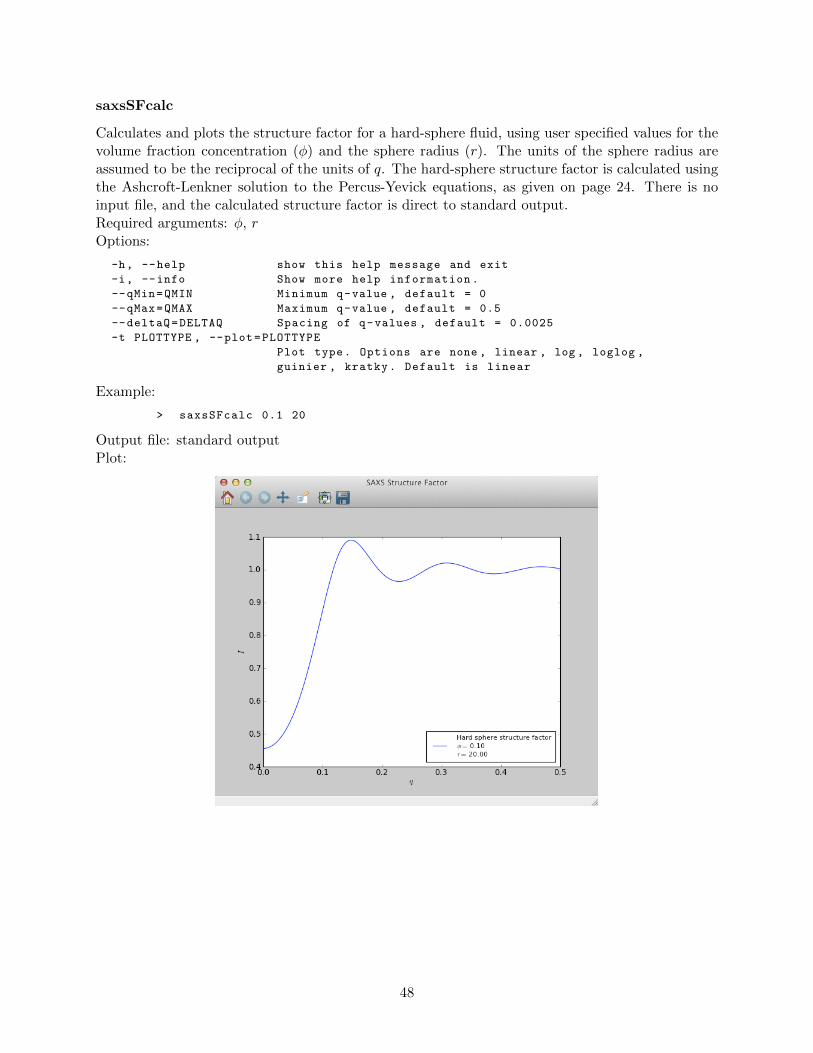
saxsSFcalc
Calculates and plots the structure factor for a hard-sphere fluid, using user specified values for thevolume fraction concentration (φ) and the sphere radius (r). The units of the sphere radius areassumed to be the reciprocal of the units of q. The hard-sphere structure factor is calculated usingthe Ashcroft-Lenkner solution to the Percus-Yevick equations, as given on page 24. There is noinput file, and the calculated structure factor is direct to standard output.Required arguments: φ, rOptions:
-h, --help show this help message and exit
-i, --info Show more help information.
--qMin=QMIN Minimum q-value , default = 0
--qMax=QMAX Maximum q-value , default = 0.5
--deltaQ=DELTAQ Spacing of q-values , default = 0.0025
-t PLOTTYPE , --plot=PLOTTYPE
Plot type. Options are none , linear , log , loglog ,
guinier , kratky. Default is linear
Example:
> saxsSFcalc 0.1 20
Output file: standard outputPlot:
48
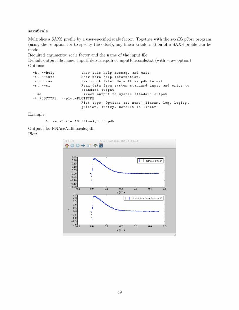
saxsScale
Multiplies a SAXS profile by a user-specified scale factor. Together with the saxsBkgCorr program(using the -c option for to specify the offset), any linear tranformation of a SAXS profile can bemade.Required arguments: scale factor and the name of the input fileDefault output file name: inputFile scale.pdh or inputFile scale.txt (with --raw option)Options:
-h, --help show this help message and exit
-i, --info Show more help information.
-r, --raw Raw input file. Default is pdh format
-s, --si Read data from system standard input and write to
standard output
--so Direct output to system standard output
-t PLOTTYPE , --plot=PLOTTYPE
Plot type. Options are none , linear , log , loglog ,
guinier , kratky. Default is linear
Example:
> saxsScale 10 RNAseA_diff.pdh
Output file: RNAseA diff scale.pdhPlot:
49
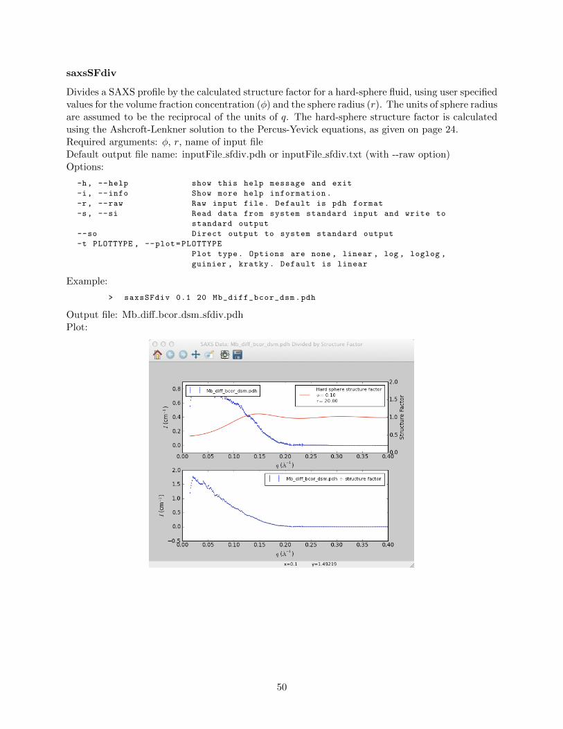
saxsSFdiv
Divides a SAXS profile by the calculated structure factor for a hard-sphere fluid, using user specifiedvalues for the volume fraction concentration (φ) and the sphere radius (r). The units of sphere radiusare assumed to be the reciprocal of the units of q. The hard-sphere structure factor is calculatedusing the Ashcroft-Lenkner solution to the Percus-Yevick equations, as given on page 24.Required arguments: φ, r, name of input fileDefault output file name: inputFile sfdiv.pdh or inputFile sfdiv.txt (with --raw option)Options:
-h, --help show this help message and exit
-i, --info Show more help information.
-r, --raw Raw input file. Default is pdh format
-s, --si Read data from system standard input and write to
standard output
--so Direct output to system standard output
-t PLOTTYPE , --plot=PLOTTYPE
Plot type. Options are none , linear , log , loglog ,
guinier , kratky. Default is linear
Example:
> saxsSFdiv 0.1 20 Mb_diff_bcor_dsm.pdh
Output file: Mb diff bcor dsm sfdiv.pdhPlot:
50
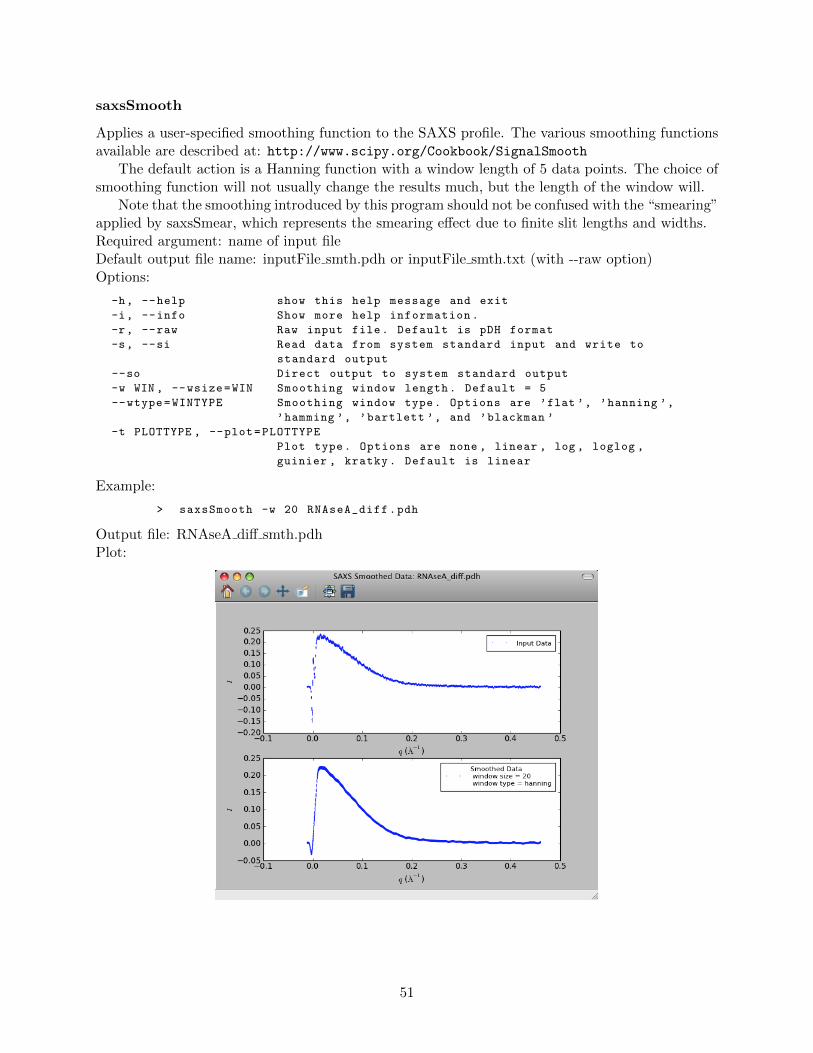
saxsSmooth
Applies a user-specified smoothing function to the SAXS profile. The various smoothing functionsavailable are described at: http://www.scipy.org/Cookbook/SignalSmooth
The default action is a Hanning function with a window length of 5 data points. The choice ofsmoothing function will not usually change the results much, but the length of the window will.
Note that the smoothing introduced by this program should not be confused with the “smearing”applied by saxsSmear, which represents the smearing effect due to finite slit lengths and widths.Required argument: name of input fileDefault output file name: inputFile smth.pdh or inputFile smth.txt (with --raw option)Options:
-h, --help show this help message and exit
-i, --info Show more help information.
-r, --raw Raw input file. Default is pDH format
-s, --si Read data from system standard input and write to
standard output
--so Direct output to system standard output
-w WIN , --wsize=WIN Smoothing window length. Default = 5
--wtype=WINTYPE Smoothing window type. Options are ’flat ’, ’hanning ’,
’hamming ’, ’bartlett ’, and ’blackman ’
-t PLOTTYPE , --plot=PLOTTYPE
Plot type. Options are none , linear , log , loglog ,
guinier , kratky. Default is linear
Example:
> saxsSmooth -w 20 RNAseA_diff.pdh
Output file: RNAseA diff smth.pdhPlot:
51
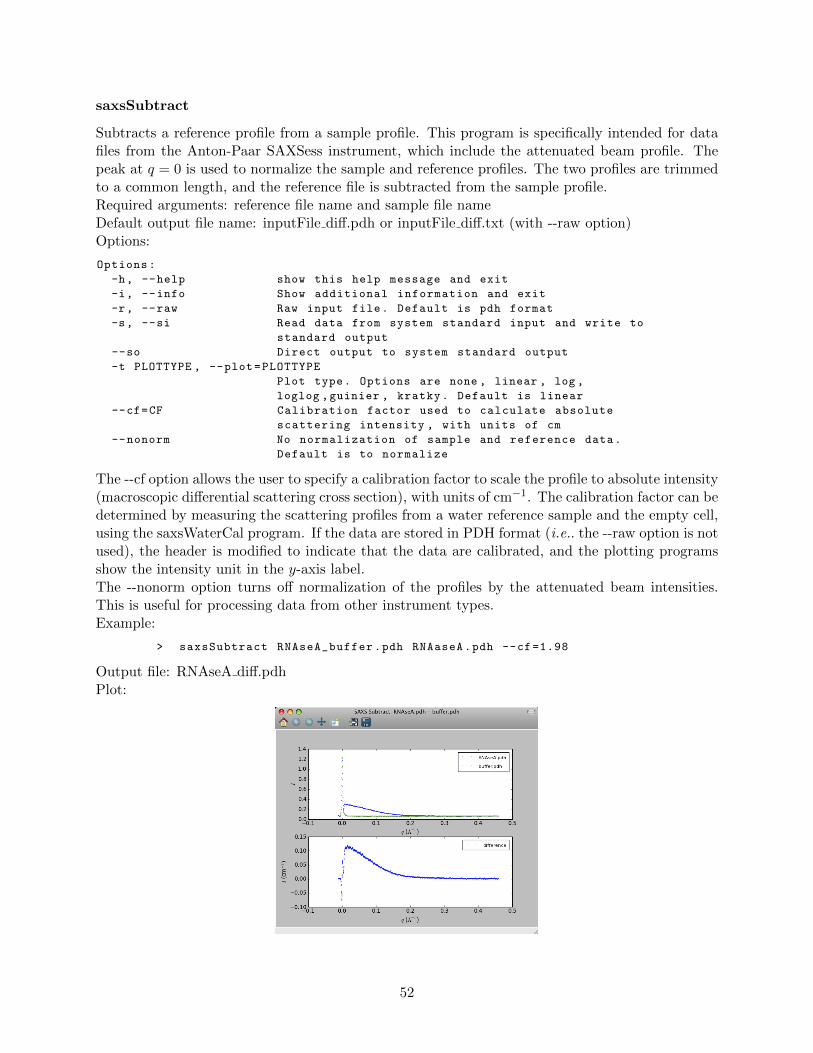
saxsSubtract
Subtracts a reference profile from a sample profile. This program is specifically intended for datafiles from the Anton-Paar SAXSess instrument, which include the attenuated beam profile. Thepeak at q = 0 is used to normalize the sample and reference profiles. The two profiles are trimmedto a common length, and the reference file is subtracted from the sample profile.Required arguments: reference file name and sample file nameDefault output file name: inputFile diff.pdh or inputFile diff.txt (with --raw option)Options:
Options:
-h, --help show this help message and exit
-i, --info Show additional information and exit
-r, --raw Raw input file. Default is pdh format
-s, --si Read data from system standard input and write to
standard output
--so Direct output to system standard output
-t PLOTTYPE , --plot=PLOTTYPE
Plot type. Options are none , linear , log ,
loglog ,guinier , kratky. Default is linear
--cf=CF Calibration factor used to calculate absolute
scattering intensity , with units of cm
--nonorm No normalization of sample and reference data.
Default is to normalize
The --cf option allows the user to specify a calibration factor to scale the profile to absolute intensity(macroscopic differential scattering cross section), with units of cm−1. The calibration factor can bedetermined by measuring the scattering profiles from a water reference sample and the empty cell,using the saxsWaterCal program. If the data are stored in PDH format (i.e.. the --raw option is notused), the header is modified to indicate that the data are calibrated, and the plotting programsshow the intensity unit in the y-axis label.The --nonorm option turns off normalization of the profiles by the attenuated beam intensities.This is useful for processing data from other instrument types.Example:
> saxsSubtract RNAseA_buffer.pdh RNAaseA.pdh --cf=1.98
Output file: RNAseA diff.pdhPlot:
52
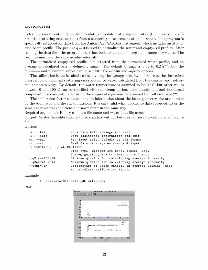
saxsWaterCal
Determines a calibration factor for calculating absolute scattering intensities (the macroscopic dif-ferential scattering cross section) from a scattering measurement of liquid water. This program isspecifically intended for data from the Anton-Paar SAXSess instrument, which includes an attenu-ated beam profile. The peak at q = 0 is used to normalize the water and empty-cell profiles. Afterreading the data files, the program first trims both to a common length and range of q-values. Thetwo files must use the same q-value intervals.
The normalized empty-cell profile is subtracted from the normalized water profile, and anaverage is calculated over a defined q-range. The default q-range is 0.05 to 0.2 A−1, but theminimum and maximum values can be set with the --qMin and --qMax options.
The calibration factor is calculated by dividing the average intensity difference by the theoreticalmacroscopic differential scattering cross section of water, calculated from the density and isother-mal compressibility. By default, the water temperature is assumed to be 20C, but other valuesbetween 0 and 100C can be specified with the –temp option. The density and and isothermalcompressibilities are calculated using the empirical equations determined by Kell (see page 22)
The calibration factor contains implicit information about the beam geometry, the attenuationby the beam stop and the cell dimensions. It is only valid when applied to data recorded under thesame experimental conditions and normalized in the same way.Required arguments: Empty-cell data file name and water data file name.Output: Writes the calibration factor to standard output, but does not save the calculated differencefile.Options:
-h, --help show this help message and exit
-i, --info Show additional information and exit
-r, --raw Raw input file. Default is pdh format
-s, --si Read data from system standard input
-t PLOTTYPE , --plot=PLOTTYPE
Plot type. Options are none , linear , log ,
loglog ,guinier , kratky. Default is linear
--qMin=AVGQMIN Minimum q-value for calculating average intensity
--qMax=AVGQMAX Maximum q-value for calculating average intensity
--temp=TEMP Temperature of water sample , in degrees Celsius , used
to calculate calibration factor
Example:
> saxsWaterCal cell.pdh water.pdh
Plot:
53
4.3.5 Advanced data processing programs
These three programs apply more complex transformations, involving smearing or desmearing, toexperimental or simulated scattering profiles and generally require more user specified parametersthan do the programs described in the previous section. Rather than using command line argumentsfor the parameters, each of these programs uses a special parameter file to specify the values. Theparameter files are simple text files with the parameter values listed on individual lines, in a specifiedorder. The files can contain blank lines and comment lines that begin with the “#” character. Eachparameter line can also contain comments following the parameter value, provided that they areseparated by the value by one or more spaces. However, the specified order of the parameter linesmust be followed.
For each of these programs, the first required command-line argument is the name of theparameter file The saxsSmear program also includes an option (invoked by the --iMode option)for the user to enter the parameters interactively. The last command-line argument is the name ofthe input file (unless the standard input option, -s or --si, is used).
saxsDeSmear
Uses the Lake algorithm to correct a SAXS profile recorded using a line-collimated beam. Theprogram can account for the beam length and width, as well as a finite detector slit width. Thelatter parameter is equivalent to the width of the integration region used for with a two-dimensionaldetector. The experimental parameters describing the beam profile and detector slit width are readfrom the header lines of the input SAXS data file, which must be in the pDH format, as describedon page 26. The other parameters for desmearing are specified in a parameter file, as describedfurther below. The buffer reference profile should be subtracted from the scattering profile beforeapplying the desmearing, and any background subtraction should be applied before desmearing.Required arguments: Name of parameter file and name of input data file (must be in pDH format)Default output file name: inputFile dsm.pdh and inputFile diff dsm.logOptions:
-h, --help show this help message and exit
-i, --info Show more help information.
-s, --si Read data from system standard input and write to standard
output
--so Direct output to system standard output
Example
> saxsDeSmear desmearParam.txt RNAseA_diff.pdh
Output files: RNAseA diff dsm.pdh and RNAseA diff dsm.log
The header of the output pDH file is modified to indicate no smearing (beam type = 0) andto correctly indicate the number of points in the desmeared profile, but the other header fieldsfrom the input file defining the beam shape and detector slit width are retained. Details of thedesmearing parameters are output to the log file.
The values specified in the parameter file are:
• Desmearing iterations. The Lake procedure is iterative, and the number of optimal number ofiterations may require adjustment. The program generates graphs that illustrate the progres-sion of the process, and these can be used to choose the total number of iterations. Only theresult of the final specified iteration is saved as the output of the program. A useful strategy
54
is to run the program with increasing numbers of iterations and then reduce the number onceit is clear that the optimum number has been exceeded (as indicated by no further reductionin the residuals or an increase in noise).
• Smoothing window length for intermediate results. By its nature, the desmearing proceduretends to enhance the noise in the profiles, and this effect increases with more iterations. Tolimit this effect, the intermediate results can be smoothed, using a window function covering aspecified number of data points. A larger window size leads to more pronounced smoothing.For no smoothing, specify a value less than 3. The degree of smoothing is a subjectiveparameter, but I suggest that the window length be adjusted so that the noise level in thefinal profile is comparable to that in the input profile.
• Smoothing window length for the final iteration. This is analogous to the parameter describedabove for the intermediate results.
• Minimum q-value for desmearing. The data for small q-values that are perturbed by the beamstop should be excluded from the desmearing calculation.
• Maximum q-value for desmearing. Data corresponding to intensities close to the baselinewill not contribute to the desmeared profile and may increase the noise level. However, alsokeep in mind that each iteration of the Lake algorithm shortens the data set by reducingthe maximum q-value. The saxsDeSmear program fills these points back in with the originalsmeared values after each iteration except the last.
• ∆q, the spacing between q-values in the output profile.
• Include beam width correction (‘y’ or ’n’). If the beam width is specified in the experimentaldata file, this parameter determines whether or not the correction is applied. If no beamwidth is specified in the data file, no correction will be applied regardless of this parameter.The beam width correction is usually very small, relative to the beam length correction, andit adds greatly to the computational time, since it increases the number of dimensions overwhich the data must be integrated from one to two.
• Minimum q-value for plotting.
• Maximum q-value for plotting.
• Minimum I-value for plotting.
• Maximum I-value for plotting.
• Plot type: ‘linear’, ‘log’, ‘loglog’, ’guinier’ or ’kratky’
• Plot the smearing functions (‘y’ or ‘n’)
• Show the plots on the screen (‘y’ or ‘n’). One might want to turn off the plots when processingseveral similar profiles in a batch process.
• Save the plots to a graphics file (‘y’ or ‘n’).
• Image format for plots: ‘emf’,‘eps’,‘pdf’,‘png’,‘ps’,‘raw’,‘rgba‘,‘svg‘,’svgz’
A sample parameter file is listed below:
# SAXS desmearing parameters
3 # desmearing iterations
15 # smoothing window for intermediate results (odd integer)
1 # smoothing window for result of last iteration (odd integer)
0.02 # q min for desmearing
55

0.4 # q max for desmearing
0.001 # delta q for desmeared curve
n # include beam width correction: ’y’ or ’n’
# Plot limits
0.0 # q min for plotting
0.6 # q max for plotting
1E-3 # i min for plotting
1 # i max for plotting
# Plot options
log # plot type: "linear", "log", "loglog", "guinier" or "kratky"
n # plot smear functions: ’y’ or ’n’
y # Show plots (on screen ): ’y’ or ’n’
n # Save plots: ’y’ or ’n’
pdf # Image format for plots
Running the saxsDeSmear program generates a four-paneled figure (unless the “show plots” pa-rameter is set to ‘n’), as shown below:
The upper left panel shows the result of each desmearing iteration along with the original experi-mental data. The upper right panel also shows the original data, along with the result of applyingthe smearing convolution to each of the desmeared profiles. The progress of the process is indicatedby the agreement (or lack thereof) between the experimental data and the smeared-desmeared pro-file. In this case, it is clear that there is a quite good agreement after the first iteration. The two
56
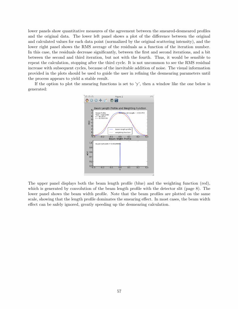
lower panels show quantitative measures of the agreement between the smeared-desmeared profilesand the original data. The lower left panel shows a plot of the difference between the originaland calculated values for each data point (normalized by the original scattering intensity), and thelower right panel shows the RMS average of the residuals as a function of the iteration number.In this case, the residuals decrease significantly, between the first and second iterations, and a bitbetween the second and third iteration, but not with the fourth. Thus, it would be sensible torepeat the calculation, stopping after the third cycle. It is not uncommon to see the RMS residualincrease with subsequent cycles, because of the inevitable addition of noise. The visual informationprovided in the plots should be used to guide the user in refining the desmearing parameters untilthe process appears to yield a stable result.
If the option to plot the smearing functions is set to ’y’, then a window like the one below isgenerated:
The upper panel displays both the beam length profile (blue) and the weighting function (red),which is generated by convolution of the beam length profile with the detector slit (page 8). Thelower panel shows the beam width profile. Note that the beam profiles are plotted on the samescale, showing that the length profile dominates the smearing effect. In most cases, the beam widtheffect can be safely ignored, greatly speeding up the desmearing calculation.
57
saxsFit
Fits experimental data to model scattering profiles, such as generated by the program CRYSOL(http://www.embl-hamburg.de/biosaxs/crysol.html). The program includes a provision to usesmeared experimental data. Rather than desmearing the experimental data, the program smearsthe model data and compares this directly with the experimental data. The only required fittingparameter is a scaling constant to match the intensity of the model data to the experimental data.Optionally, an intensity offset parameter can be introduced and allowed to float. In addition, thetheoretical structure factor for a solution of hard spheres, based on the equations on page 24, canbe incorporated, with up to two additional fitting factors. The experimental parameters describingthe beam profile and detector slit width are read from the header lines of the input SAXS datafile, which must be in the pDH format, as described on page 26. The model data are provided ina separate file, described below. The other parameters for desmearing are specified in a parameterfile, also described below.
Required arguments: Name of parameter file, name of model SAXS data file and name of inputdata fileOptions:
-h, --help show this help message and exit
-i, --info Show more help information.
-s, --si Read data from system standard input and write to standard
output
--so Direct output to system standard output
The values specified in the parameter file are:
• Minimum q-value for fitting
• Maximum q-value for fitting
• Include beam width correction (‘y’ or ’n’). If the beam width is specified in the experimentaldata file, this parameter determines whether or not the correction is applied. If no beamwidth is specified in the data file, no correction will be applied regardless of this parameter.The beam width correction is usually very small, relative to the beam length correction, andit adds greatly to the computational time, since it increases the number of dimensions overwhich the data must be integrated from one to two.
• Allow background correction (’y’ or ’n’). This introduces a floating offset parameter in theleast-squares fitting.
• Fit to a linear combination of the first two models in the model file (‘y’ or ’n’).
• Specified fraction of the first model in the linear combination. Allow to float if 0.
• Include hard-sphere structure factor in fit (‘y’ or ’n’).
• Specified volume-fraction concentration, 0 < φ < 1, for hard-sphere structure factor. Allowto float in fitting if 0.
• Specified sphere radius, r, for hard-sphere structure factor. Allow to float in fitting if 0.
• Minimum q-value for plotting.
• Maximum q-value for plotting.
• Minimum I-value for plotting.
58
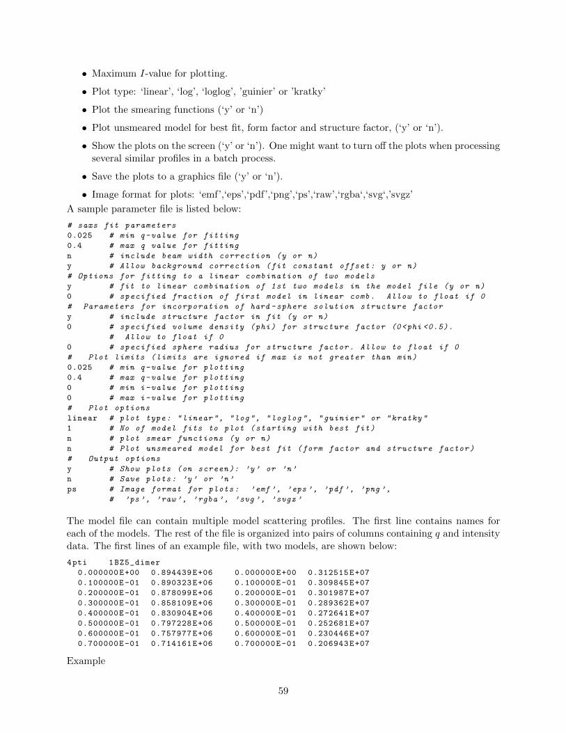
• Maximum I-value for plotting.
• Plot type: ‘linear’, ‘log’, ‘loglog’, ’guinier’ or ’kratky’
• Plot the smearing functions (‘y’ or ‘n’)
• Plot unsmeared model for best fit, form factor and structure factor, (‘y’ or ‘n’).
• Show the plots on the screen (‘y’ or ‘n’). One might want to turn off the plots when processingseveral similar profiles in a batch process.
• Save the plots to a graphics file (‘y’ or ‘n’).
• Image format for plots: ‘emf’,‘eps’,‘pdf’,‘png’,‘ps’,‘raw’,‘rgba‘,‘svg‘,’svgz’
A sample parameter file is listed below:
# saxs fit parameters
0.025 # min q-value for fitting
0.4 # max q value for fitting
n # include beam width correction (y or n)
y # Allow background correction (fit constant offset: y or n)
# Options for fitting to a linear combination of two models
y # fit to linear combination of 1st two models in the model file (y or n)
0 # specified fraction of first model in linear comb. Allow to float if 0
# Parameters for incorporation of hard -sphere solution structure factor
y # include structure factor in fit (y or n)
0 # specified volume density (phi) for structure factor (0<phi <0.5).
# Allow to float if 0
0 # specified sphere radius for structure factor. Allow to float if 0
# Plot limits (limits are ignored if max is not greater than min)
0.025 # min q-value for plotting
0.4 # max q-value for plotting
0 # min i-value for plotting
0 # max i-value for plotting
# Plot options
linear # plot type: "linear", "log", "loglog", "guinier" or "kratky"
1 # No of model fits to plot (starting with best fit)
n # plot smear functions (y or n)
n # Plot unsmeared model for best fit (form factor and structure factor)
# Output options
y # Show plots (on screen ): ’y’ or ’n’
n # Save plots: ’y’ or ’n’
ps # Image format for plots: ’emf ’, ’eps ’, ’pdf ’, ’png ’,
# ’ps’, ’raw ’, ’rgba ’, ’svg ’, ’svgz ’
The model file can contain multiple model scattering profiles. The first line contains names foreach of the models. The rest of the file is organized into pairs of columns containing q and intensitydata. The first lines of an example file, with two models, are shown below:
4pti 1BZ5_dimer
0.000000E+00 0.894439E+06 0.000000E+00 0.312515E+07
0.100000E-01 0.890323E+06 0.100000E-01 0.309845E+07
0.200000E-01 0.878099E+06 0.200000E-01 0.301987E+07
0.300000E-01 0.858109E+06 0.300000E-01 0.289362E+07
0.400000E-01 0.830904E+06 0.400000E-01 0.272641E+07
0.500000E-01 0.797228E+06 0.500000E-01 0.252681E+07
0.600000E-01 0.757977E+06 0.600000E-01 0.230446E+07
0.700000E-01 0.714161E+06 0.700000E-01 0.206943E+07
Example
59
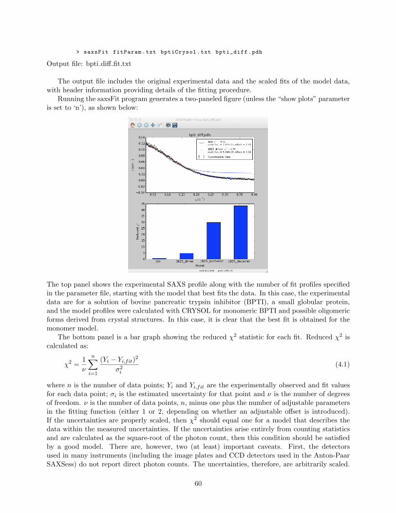
> saxsFit fitParam.txt bptiCrysol.txt bpti_diff.pdh
Output file: bpti diff fit.txt
The output file includes the original experimental data and the scaled fits of the model data,with header information providing details of the fitting procedure.
Running the saxsFit program generates a two-paneled figure (unless the “show plots” parameteris set to ‘n’), as shown below:
The top panel shows the experimental SAXS profile along with the number of fit profiles specifiedin the parameter file, starting with the model that best fits the data. In this case, the experimentaldata are for a solution of bovine pancreatic trypsin inhibitor (BPTI), a small globular protein,and the model profiles were calculated with CRYSOL for monomeric BPTI and possible oligomericforms derived from crystal structures. In this case, it is clear that the best fit is obtained for themonomer model.
The bottom panel is a bar graph showing the reduced χ2 statistic for each fit. Reduced χ2 iscalculated as:
χ2 =1
ν
n∑i=1
(Yi − Yi,fit)2
σ2i
(4.1)
where n is the number of data points; Yi and Yi,fit are the experimentally observed and fit valuesfor each data point; σi is the estimated uncertainty for that point and ν is the number of degreesof freedom. ν is the number of data points, n, minus one plus the number of adjustable parametersin the fitting function (either 1 or 2, depending on whether an adjustable offset is introduced).If the uncertainties are properly scaled, then χ2 should equal one for a model that describes thedata within the measured uncertainties. If the uncertainties arise entirely from counting statisticsand are calculated as the square-root of the photon count, then this condition should be satisfiedby a good model. There are, however, two (at least) important caveats. First, the detectorsused in many instruments (including the image plates and CCD detectors used in the Anton-PaarSAXSess) do not report direct photon counts. The uncertainties, therefore, are arbitrarily scaled.
60
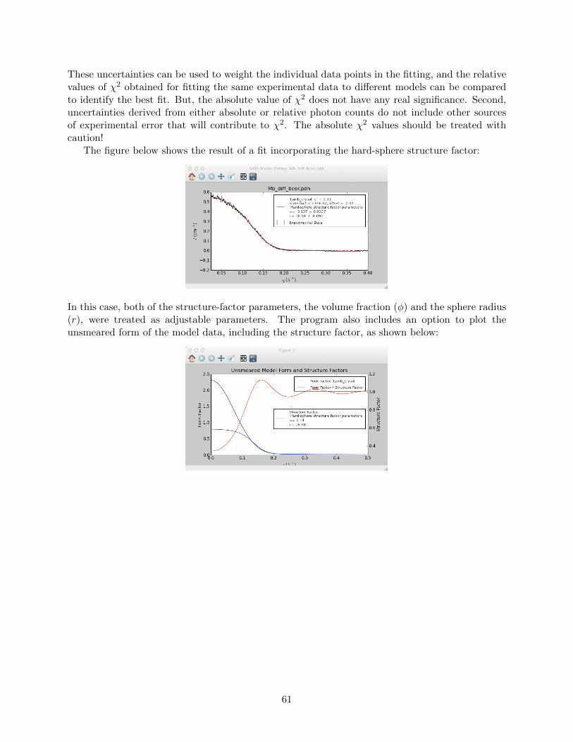
These uncertainties can be used to weight the individual data points in the fitting, and the relativevalues of χ2 obtained for fitting the same experimental data to different models can be comparedto identify the best fit. But, the absolute value of χ2 does not have any real significance. Second,uncertainties derived from either absolute or relative photon counts do not include other sourcesof experimental error that will contribute to χ2. The absolute χ2 values should be treated withcaution!
The figure below shows the result of a fit incorporating the hard-sphere structure factor:
In this case, both of the structure-factor parameters, the volume fraction (φ) and the sphere radius(r), were treated as adjustable parameters. The program also includes an option to plot theunsmeared form of the model data, including the structure factor, as shown below:
61
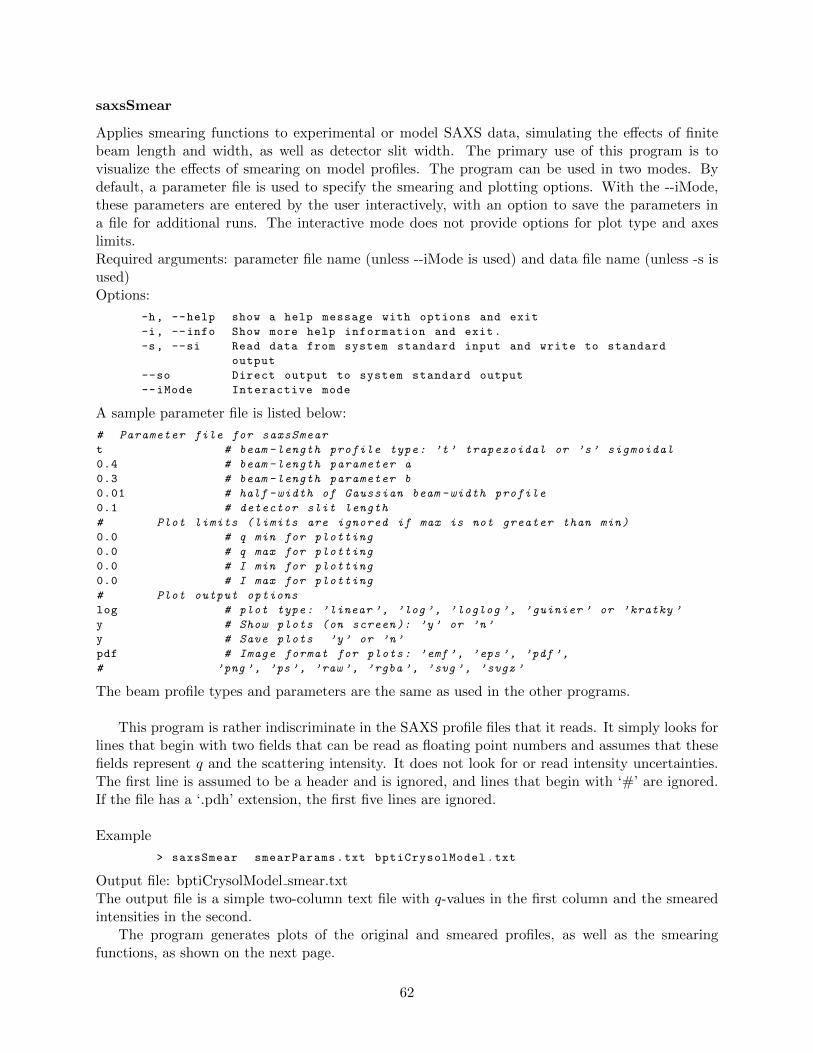
saxsSmear
Applies smearing functions to experimental or model SAXS data, simulating the effects of finitebeam length and width, as well as detector slit width. The primary use of this program is tovisualize the effects of smearing on model profiles. The program can be used in two modes. Bydefault, a parameter file is used to specify the smearing and plotting options. With the --iMode,these parameters are entered by the user interactively, with an option to save the parameters ina file for additional runs. The interactive mode does not provide options for plot type and axeslimits.Required arguments: parameter file name (unless --iMode is used) and data file name (unless -s isused)Options:
-h, --help show a help message with options and exit
-i, --info Show more help information and exit.
-s, --si Read data from system standard input and write to standard
output
--so Direct output to system standard output
--iMode Interactive mode
A sample parameter file is listed below:
# Parameter file for saxsSmear
t # beam -length profile type: ’t’ trapezoidal or ’s’ sigmoidal
0.4 # beam -length parameter a
0.3 # beam -length parameter b
0.01 # half -width of Gaussian beam -width profile
0.1 # detector slit length
# Plot limits (limits are ignored if max is not greater than min)
0.0 # q min for plotting
0.0 # q max for plotting
0.0 # I min for plotting
0.0 # I max for plotting
# Plot output options
log # plot type: ’linear ’, ’log ’, ’loglog ’, ’guinier ’ or ’kratky ’
y # Show plots (on screen ): ’y’ or ’n’
y # Save plots ’y’ or ’n’
pdf # Image format for plots: ’emf ’, ’eps ’, ’pdf ’,
# ’png ’, ’ps ’, ’raw ’, ’rgba ’, ’svg ’, ’svgz ’
The beam profile types and parameters are the same as used in the other programs.
This program is rather indiscriminate in the SAXS profile files that it reads. It simply looks forlines that begin with two fields that can be read as floating point numbers and assumes that thesefields represent q and the scattering intensity. It does not look for or read intensity uncertainties.The first line is assumed to be a header and is ignored, and lines that begin with ‘#’ are ignored.If the file has a ‘.pdh’ extension, the first five lines are ignored.
Example
> saxsSmear smearParams.txt bptiCrysolModel.txt
Output file: bptiCrysolModel smear.txtThe output file is a simple two-column text file with q-values in the first column and the smearedintensities in the second.
The program generates plots of the original and smeared profiles, as well as the smearingfunctions, as shown on the next page.
62
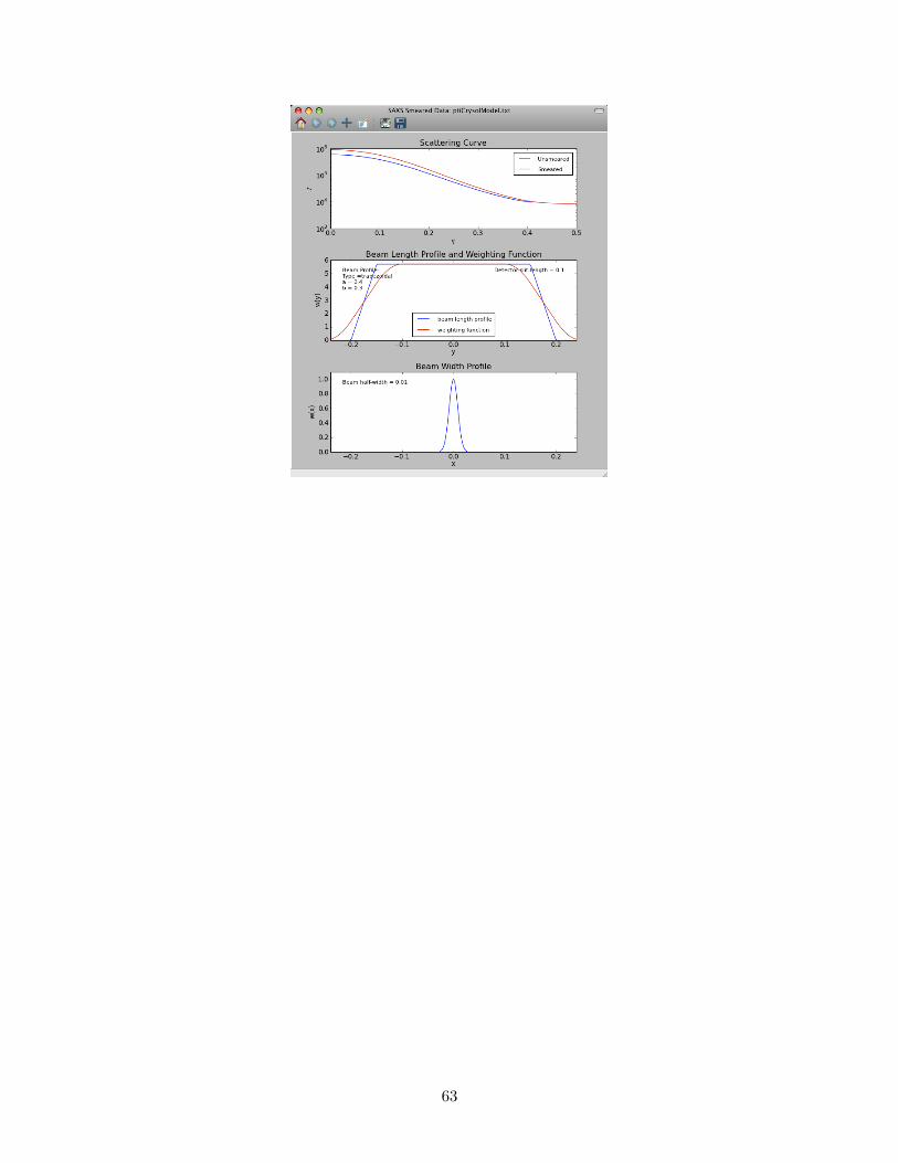
63
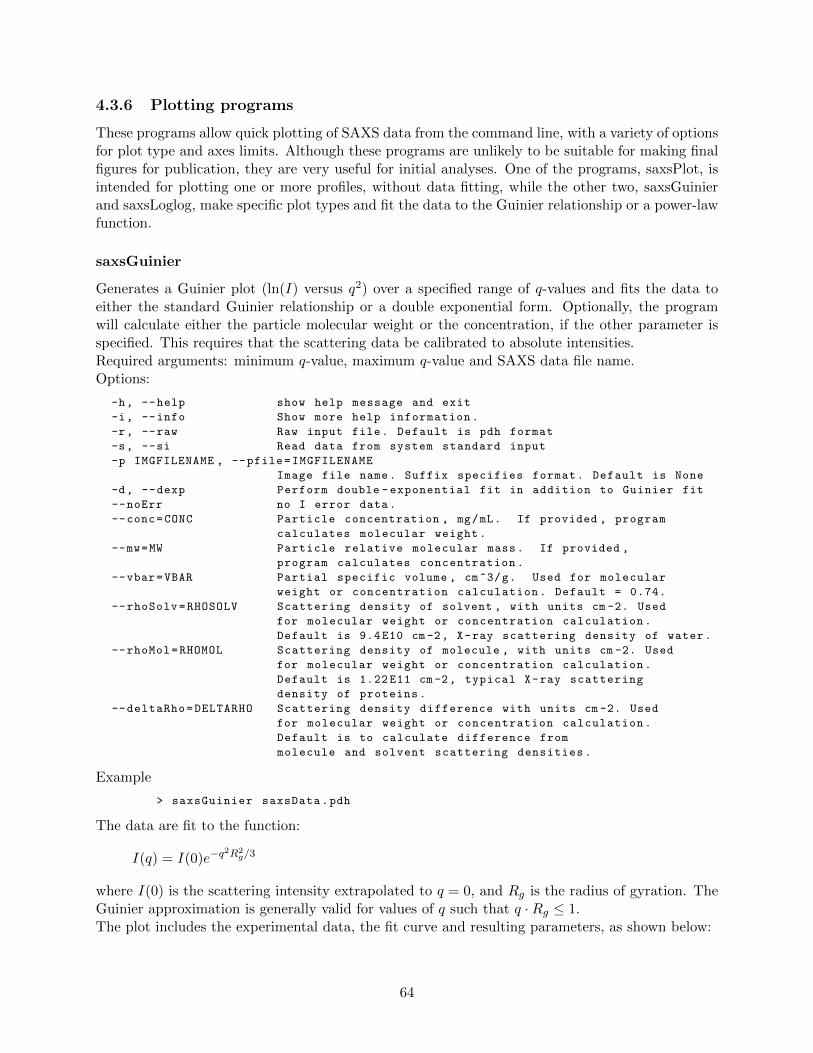
4.3.6 Plotting programs
These programs allow quick plotting of SAXS data from the command line, with a variety of optionsfor plot type and axes limits. Although these programs are unlikely to be suitable for making finalfigures for publication, they are very useful for initial analyses. One of the programs, saxsPlot, isintended for plotting one or more profiles, without data fitting, while the other two, saxsGuinierand saxsLoglog, make specific plot types and fit the data to the Guinier relationship or a power-lawfunction.
saxsGuinier
Generates a Guinier plot (ln(I) versus q2) over a specified range of q-values and fits the data toeither the standard Guinier relationship or a double exponential form. Optionally, the programwill calculate either the particle molecular weight or the concentration, if the other parameter isspecified. This requires that the scattering data be calibrated to absolute intensities.Required arguments: minimum q-value, maximum q-value and SAXS data file name.Options:
-h, --help show help message and exit
-i, --info Show more help information.
-r, --raw Raw input file. Default is pdh format
-s, --si Read data from system standard input
-p IMGFILENAME , --pfile=IMGFILENAME
Image file name. Suffix specifies format. Default is None
-d, --dexp Perform double -exponential fit in addition to Guinier fit
--noErr no I error data.
--conc=CONC Particle concentration , mg/mL. If provided , program
calculates molecular weight.
--mw=MW Particle relative molecular mass. If provided ,
program calculates concentration.
--vbar=VBAR Partial specific volume , cm^3/g. Used for molecular
weight or concentration calculation. Default = 0.74.
--rhoSolv=RHOSOLV Scattering density of solvent , with units cm -2. Used
for molecular weight or concentration calculation.
Default is 9.4 E10 cm -2, X-ray scattering density of water.
--rhoMol=RHOMOL Scattering density of molecule , with units cm -2. Used
for molecular weight or concentration calculation.
Default is 1.22 E11 cm -2, typical X-ray scattering
density of proteins.
--deltaRho=DELTARHO Scattering density difference with units cm -2. Used
for molecular weight or concentration calculation.
Default is to calculate difference from
molecule and solvent scattering densities.
Example
> saxsGuinier saxsData.pdh
The data are fit to the function:
I(q) = I(0)e−q2R2
g/3
where I(0) is the scattering intensity extrapolated to q = 0, and Rg is the radius of gyration. TheGuinier approximation is generally valid for values of q such that q ·Rg ≤ 1.The plot includes the experimental data, the fit curve and resulting parameters, as shown below:
64
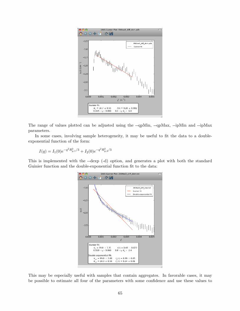
The range of values plotted can be adjusted using the --qpMin, --qpMax, --ipMin and --ipMaxparameters.
In some cases, involving sample heterogeneity, it may be useful to fit the data to a double-exponential function of the form:
I(q) = I1(0)e−q2R2
g,1/3 + I2(0)e−q2R2
g,2/3
This is implemented with the --dexp (-d) option, and generates a plot with both the standardGuinier function and the double-exponential function fit to the data:
This may be especially useful with samples that contain aggregates. In favorable cases, it maybe possible to estimate all four of the parameters with some confidence and use these values to
65
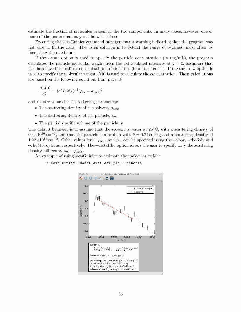
estimate the fraction of molecules present in the two components. In many cases, however, one ormore of the parameters may not be well defined.
Executing the saxsGuinier command may generate a warning indicating that the program wasnot able to fit the data. The usual solution is to extend the range of q-values, most often byincreasing the maximum.
If the --conc option is used to specify the particle concentration (in mg/mL), the programcalculates the particle molecular weight from the extrapolated intensity at q = 0, assuming thatthe data have been calibrated to absolute in intensities (in units of cm−1). If the the --mw option isused to specify the molecular weight, I(0) is used to calculate the concentration. These calculationsare based on the following equation, from page 18:
dΣ(0)
dΩ= (cM/NA)v2(ρm − ρsolv)2
and require values for the following parameters:
• The scattering density of the solvent, ρsolv
• The scattering density of the particle, ρm
• The partial specific volume of the particle, v
The default behavior is to assume that the solvent is water at 25C, with a scattering density of9.4×1010 cm−2, and that the particle is a protein with v = 0.74 cm3/g and a scattering density of1.22×1011 cm−2. Other values for v, ρsolv and ρm can be specified using the --vbar, --rhoSolv and--rhoMol options, respectively. The --deltaRho option allows the user to specify only the scatteringdensity difference, ρm − ρsolv.
An example of using saxsGuinier to estimate the molecular weight:
> saxsGuinier RNAseA_diff_dsm.pdh --conc =15
66
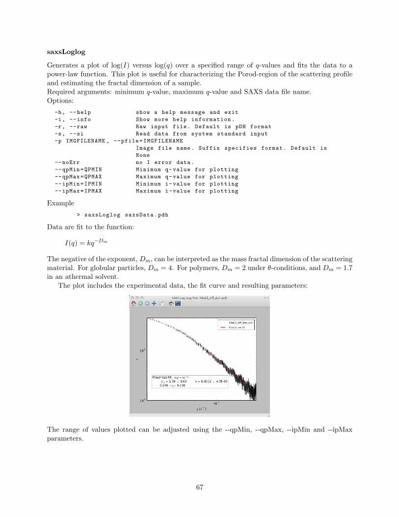
saxsLoglog
Generates a plot of log(I) versus log(q) over a specified range of q-values and fits the data to apower-law function. This plot is useful for characterizing the Porod-region of the scattering profileand estimating the fractal dimension of a sample.Required arguments: minimum q-value, maximum q-value and SAXS data file name.Options:
-h, --help show a help message and exit
-i, --info Show more help information.
-r, --raw Raw input file. Default is pDH format
-s, --si Read data from system standard input
-p IMGFILENAME , --pfile=IMGFILENAME
Image file name. Suffix specifies format. Default is
None
--noErr no I error data.
--qpMin=QPMIN Minimum q-value for plotting
--qpMax=QPMAX Maximum q-value for plotting
--ipMin=IPMIN Minimum i-value for plotting
--ipMax=IPMAX Maximum i-value for plotting
Example
> saxsLoglog saxsData.pdh
Data are fit to the function:
I(q) = kq−Dm
The negative of the exponent, Dm, can be interpreted as the mass fractal dimension of the scatteringmaterial. For globular particles, Dm = 4. For polymers, Dm = 2 under θ-conditions, and Dm = 1.7in an athermal solvent.
The plot includes the experimental data, the fit curve and resulting parameters:
The range of values plotted can be adjusted using the --qpMin, --qpMax, --ipMin and --ipMaxparameters.
67
saxsPlot
Plots SAXS data in a variety of formats, with user options to control the axes ranges and otherproperties. : Required arguments: one or more SAXS data files, in pDH or generic format (with--raw (-r) option.)Options:
-h, --help show this help message and exit
-i, --info Show more help information.
-r, --raw Raw input file. Default is pDH format
-s, --si Read data from system standard input
-p IMGFILENAME , --pfile=IMGFILENAME
Image file name. Suffix specifies format. Default is
None
-t PLOTTYPE , --type=PLOTTYPE
Plot type. Options are linear , log , loglog , guinier ,
kratky. Default is log.
--noErr no I error data.
--qMin=QMIN Minimum q-value for plotting
--qMax=QMAX Maximum q-value for plotting
--iMin=IMIN Minimum i-value for plotting
--iMax=IMAX Maximum i-value for plotting
Example
> saxsPlot saxsData.pdh
This program is described in more detail on pages 36–39, where it is used an example to illustratethe Unix interface to the USToo Python programs.
68
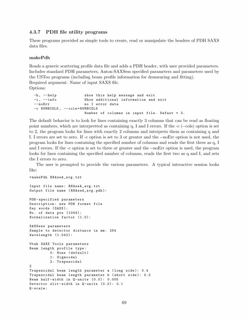
4.3.7 PDH file utility programs
These programs provided as simple tools to create, read or manipulate the headers of PDH SAXSdata files.
makePdh
Reads a generic scattering profile data file and adds a PDH header, with user provided parameters.Includes standard PDH parameters, Anton-SAXSess specified parameters and parameters used bythe USToo programs (including beam profile information for desmearing and fitting).Required argument: Name of input SAXS file.Options:
-h, --help show this help message and exit
-i, --info Show additional information and exit
--noErr no I error data
-c NUMBCOLS , --cols=NUMBCOLS
Number of columns in input file. Defaut = 3.
The default behavior is to look for lines containing exactly 3 columns that can be read as floatingpoint numbers, which are interpretted as containing q, I and I errors. If the -c (--cols) option is setto 2, the program looks for lines with exactly 2 columns and interprets them as containing q andI. I errors are set to zero. If -c option is set to 3 or greater and the --noErr option is not used, theprogram looks for lines containing the specified number of columns and reads the first three as q, Iand I errors. If the -c option is set to three or greater and the --noErr option is used, the programlooks for lines containing the specified number of columns, reads the first two as q and I, and setsthe I errors to zero.
The user is prompted to provide the various parameters. A typical interactive session lookslike:
>makePdh RNAseA_avg.txt
Input file name: RNAseA_avg.txt
Output file name (RNAseA_avg.pdh):
PDH -specified parameters
Description: new PDH format file
Key words (SAXS):
No. of data pts (1044):
Normalization factor (1.0):
SAXSess parameters
Sample to detector distance in mm: 254
Wavelength (1.542):
Utah SAXS Tools parameters
Beam length profile type:
0: None (default)
1: Sigmoidal
2: Trapezoidal
2
Trapezoidal beam length parameter a (long side): 0.4
Trapezoidal beam length parameter b (short side): 0.3
Beam half -width in Q-units (0.0): 0.005
Detector slit -width in Q-units (0.0): 0.1
Q-scale:
69
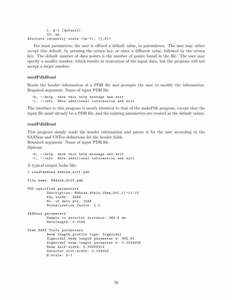
1: A-1 (default)
10: nm
Absolute intensity scale (cm -1), (y,N)?
For most parameters, the user is offered a default value, in parentheses. The user may eitheraccept this default, by pressing the return key, or enter a different value, followed by the returnkey. The default number of data points is the number of points found in the file. The user mayspecify a smaller number, which results in truncation of the input data, but the program will notaccept a larger number.
modPdhHead
Reads the header information of a PDH file and prompts the user to modify the information.Required argument: Name of input PDH file.
-h, --help show this help message and exit
-i, --info Show additional information and exit
The interface to this program is nearly identical to that of the makePdh program, except that theinput file must already be a PDH file, and the existing parameters are treated as the default values.
readPdhHead
This program simply reads the header information and parses it for the user according to theSAXSess and USToo definitions for the header fields.Required argument: Name of input PDH file.Options:
-h, --help show this help message and exit
-i, --info Show additional information and exit
A typical output looks like:
> readPdhHead RNAseA_diff.pdh
File name: RNAseA_diff.pdh
PCG -specified parameters
Description: RNAseA_30min_10mm_20C_11 -11-10
Key words: SAXS
No. of data pts: 1048
Normalization factor: 1.0
SAXSess parameters
Sample to detector distance: 264.5 mm
Wavelength: 0.1542
Utah SAXS Tools parameters
Beam length profile type: Sigmoidal
Sigmoidal beam length parameter a: 992.61
Sigmoidal beam length parameter b: 0.0204206
Beam half -width: 0.00209312
Detector slit -width: 0.154053
Q-scale: A-1
70
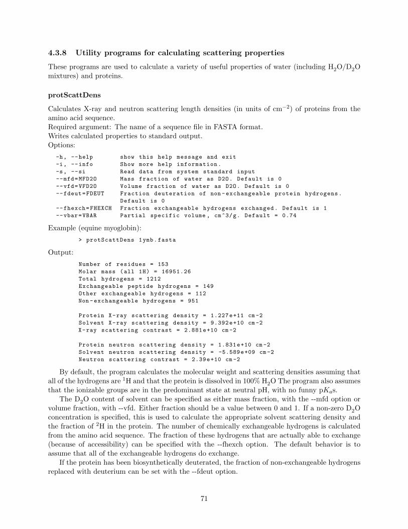
4.3.8 Utility programs for calculating scattering properties
These programs are used to calculate a variety of useful properties of water (including H2O/D2Omixtures) and proteins.
protScattDens
Calculates X-ray and neutron scattering length densities (in units of cm−2) of proteins from theamino acid sequence.Required argument: The name of a sequence file in FASTA format.Writes calculated properties to standard output.Options:
-h, --help show this help message and exit
-i, --info Show more help information.
-s, --si Read data from system standard input
--mfd=MFD2O Mass fraction of water as D2O. Default is 0
--vfd=VFD2O Volume fraction of water as D2O. Default is 0
--fdeut=FDEUT Fraction deuteration of non -exchangeable protein hydrogens.
Default is 0
--fhexch=FHEXCH Fraction exchangeable hydrogens exchanged. Default is 1
--vbar=VBAR Partial specific volume , cm^3/g. Default = 0.74
Example (equine myoglobin):
> protScattDens 1ymb.fasta
Output:
Number of residues = 153
Molar mass (all 1H) = 16951.26
Total hydrogens = 1212
Exchangeable peptide hydrogens = 149
Other exchangeable hydrogens = 112
Non -exchangeable hydrogens = 951
Protein X-ray scattering density = 1.227e+11 cm -2
Solvent X-ray scattering density = 9.392e+10 cm -2
X-ray scattering contrast = 2.881e+10 cm -2
Protein neutron scattering density = 1.831e+10 cm -2
Solvent neutron scattering density = -5.589e+09 cm -2
Neutron scattering contrast = 2.39e+10 cm -2
By default, the program calculates the molecular weight and scattering densities assuming thatall of the hydrogens are 1H and that the protein is dissolved in 100% H2O The program also assumesthat the ionizable groups are in the predominant state at neutral pH, with no funny pKas.
The D2O content of solvent can be specified as either mass fraction, with the --mfd option orvolume fraction, with --vfd. Either fraction should be a value between 0 and 1. If a non-zero D2Oconcentration is specified, this is used to calculate the appropriate solvent scattering density andthe fraction of 2H in the protein. The number of chemically exchangeable hydrogens is calculatedfrom the amino acid sequence. The fraction of these hydrogens that are actually able to exchange(because of accessibility) can be specified with the --fhexch option. The default behavior is toassume that all of the exchangeable hydrogens do exchange.
If the protein has been biosynthetically deuterated, the fraction of non-exchangeable hydrogensreplaced with deuterium can be set with the --fdeut option.
71
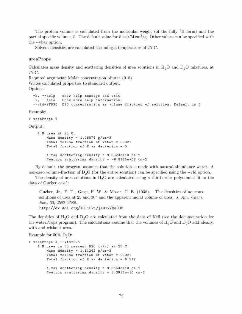
The protein volume is calculated from the molecular weight (of the fully 1H form) and thepartial specific volume, v. The default value for v is 0.74 cm3/g. Other values can be specified withthe --vbar option.
Solvent densities are calculated assuming a temperature of 25C.
ureaProps
Calculates mass density and scattering densities of urea solutions in H2O and D2O mixtures, at25C.Required argument: Molar concentration of urea (0–8)Writes calculated properties to standard output.Options:
-h, --help show help message and exit
-i, --info Show more help information.
--vfd=VFD2O D2O concentration as volume fraction of solution. Default is 0
Example:
> ureaProps 4
Output:
4 M urea at 25 C:
Mass density = 1.05874 g/cm -3
Total volume fraction of water = 0.821
Total fraction of H as deuterium = 0
X-ray scattering density = 9.8823e+10 cm -2
Neutron scattering density = -6.8325e+08 cm -2
By default, the program assumes that the solution is made with natural-abundance water. Anon-zero volume-fraction of D2O (for the entire solution) can be specified using the --vfd option.
The density of urea solutions in H2O are calculated using a third-order polynomial fit to thedata of Gucker et al.:
Gucker, Jr., F. T., Gage, F. W. & Moser, C. E. (1938). The densities of aqueoussolutions of urea at 25 and 30 and the apparent molal volume of urea. J. Am. Chem.Soc., 60, 2582–2588.http://dx.doi.org/10.1021/ja01278a008
The densities of H2O and D2O are calculated from the data of Kell (see the documentation forthe waterProps program). The calculations assume that the volumes of H2O and D2O add ideally,with and without urea.
Example for 50% D2O:
> ureaProps 4 --vfd =0.5
4 M urea in 50 percent D2O (v/v) at 25 C:
Mass density = 1.11242 g/cm -3
Total volume fraction of water = 0.821
Total fraction of H as deuterium = 0.517
X-ray scattering density = 9.8653e+10 cm -2
Neutron scattering density = 3.3913e+10 cm -2
72
waterProps
Calculates mass density and scattering densities of H2O and D2O mixtures, at temperatures be-tween 0 and 100C.Required argument: Temperature, in CWrites calculated properties to standard output.Options:
-h, --help show help message and exit
-i, --info Show more help information.
--mfd=MFD2O Mass fraction of water as D2O. Default is 0
--vfd=VFD2O Volume fraction of water as D2O. Default is 0
Example:
> waterProps 20 --vfd =0.5
Output:
50 percent D2O (v/v) at 20 C:
Mass fraction D2O = 52.5 percent
Mass density = 1.05177 g/cm -3
X-ray scattering density = 9.3843e+10 cm -2
Neutron scattering density = 2.9032e+10 cm -2
By default, the program assumes that the sample is natural-abundance water. A non-zerovolume- or mass-fraction of D2O can be specified using the --vfd or --mfd options, respectively.
The temperature-dependent densities of H2O and D2O are calculated from the data and em-pirical functions of Kell:
Kell, G. S. (1975). Density, thermal expansivity, and compressibility of liquid waterfrom 0 to 150 C: Correlations and tables for atmospheric pressure and saturationreviewed and expressed on 1968 temperature scale. J. Chem. Eng. Data, 20, 97–105.http://dx.doi.org/10.1021/je60064a005
Kell, G. S. (1967). Precise representation of volume properties of water at one atmo-sphere. J. Chem. Eng. Data, 12, 66–69.http://dx.doi.org/10.1021/je60032a018
The calculations assume that the volumes of H2O and D2O add ideally. For justification of thisassumption, see:
Bottomley, G. A. & Scott, R. L. (1976). Excess volumes for H2O + D2O mixtures.Aust. J. Chem., 29, 427–428.http://dx.doi.org/10.1071/CH9760427
73
4.3.9 Simple shell scripts for data processing
The USToo Python programs, like other programs that can be executed from a Unix shell, canalso be included in shell scripts, providing a means of automating data processing. A shell scriptis simply a text file containing commands that are executed sequentially when the script, itself, isexecuted. Shell scripts can be very simple or quite sophisticated, and even a rudimentary treatmentis beyond the scope of this document. The examples provided here are only meant to be a startingpoint, and much more information can be found on the internet.The following is a simple script that does a background subtraction, bins the data, desmears it andthen generates a Guinier plot:
#! /bin/bash
saxsSubtract RNAseA_buffer.pdh RNAseA.pdh
saxsBinData -n 5 RNAseA_diff.pdh
saxsDeSmear desmearParam.txt RNAseA_diff_bin.pdh
saxsGuinier 0.03 0.06 RNAseA_diff_bin_dsm.pdh
The first line identifies the script as being targeted to the bash shell. There are several differentshell environments in the Unix world, each with its own peculiarities and syntax. The bash shellis widely used as the default for both Linux and Mac OS X systems, but others are also available.Each line in the script above executes one of the USToo programs, just as if the line were typed atthe shell prompt. The script takes advantage of the default naming scheme used by the programs,so that the name of each output file can be used for the input to the next command. The scriptassumes that the starting files, RNAseA buffer.pdh and RNAseA.pdh, as well as the desmearingparameter file (desmearParam.txt), are in the same directory as the script when it is executed.Another important detail is that the final line must include a “line feed” character, created bypressing the return key, so that the final command will be executed. This creates a blank line atthe end of the file.
By convention, shell scripts are saved with the extension “.sh”, so that this script might besaved as process.sh. After saving the script, it can be executed with the Unix source command:
> source process.sh
This will cause each of the commands to executed in turn. Each program generates a plot windowand pauses until the window is closed. Thus, the programs wait for the user to dismiss the resultfrom the previous one.
Shell scripts can also be made to behave like shell commands by setting the executable bit withthe chmod command. The following command will make the script executable by its owner:
> chmod u+x process.sh
After this is done the script can be executed simply by typing:
> process.sh
If you prefer not to see the intermediate results of the processing steps, the “none” plot typeoption can be used:
#! /bin/bash
saxsSubtract RNAseA_buffer.pdh RNAseA.pdh -t none
saxsBinData -n 5 RNAseA_diff.pdh -t none
saxsDeSmear desmearParam.txt RNAseA_diff_bin.pdh
saxsGuinier 0.03 0.06 RNAseA_diff_bin_dsm.pdh
This suppresses the plots from saxsSubtract and saxsBinData, but the saxsDeSmear plots will stillappear, unless the appropriate setting in the parameter file is set to turn the plot display off.
74
A further refinement involves using the pipe feature of the shell to direct the output of oneprogram to the input of another, without writing the intermediate files to the disk. An example isshown below:
#! /bin/bash
saxsSubtract RNAseA_buffer.pdh RNAseA.pdh -t none --so | \
saxsBinData -n 5 --si -t none | \
saxsDeSmear desmearParam.txt --si > RNAseA_diff_bin_dsm.txt
saxsGuinier 0.03 0.06 RNAseA_diff_bin_dsm.txt
In this case, the output of the first program, saxsSubtract, is directed to standard output using the--so option and is piped to the input of the second command, saxsBinData, using the “|” symbol.This requires that the --si option be used with the saxsBinData command. Also, note the backslash(“\”) character at the ends of the first and second line. When piped commands are typed at theshell prompt, all of the commands are typed on the same line, before the return key is pressed.The backslash tells the interpreter to treat the next line as a continuation of the current line. Inthe case above the first three lines are all treated as a single line, as they would be typed at theshell prompt. In this script, the output of saxsDeSmear is directed to a new file, with the namespecified in the script, which is then used as the input to saxsGuinier.
A final example introduces the use of variables in the shell script:
#! /bin/bash
dataFileName=$1
bufferFileName="RNAseA_buffer.pdh"
rootName=$dataFileName %%.pdh
ext="_diff_bin_dsm.pdh"
outFileName="$rootName$ext"
saxsSubtract $bufferFileName $dataFileName -t none --so | \
saxsBinData -n 5 --si -t none | \
saxsDeSmear desmearParam.txt --si > $outFileName
saxsGuinier 0.03 0.06 $outFileName
In the bash shell language, the variables $1, $2, etc. correspond to arguments that are typed at thecommand line when executing the script, just as arguments for other commands are typed. In thiscase, $1 is used to allow the user to specify the data file name at the command line, so that thescript is executed by typing, for instance:
> process.sh RNAseA.pdh
The string “RNAseA.pdh” is automatically assigned to the variable $1. The role of the “$” invariable names also requires a bit of explanation. When a variables is assigned a value, it is namedwithout the “$”, but when the value assigned is later used, the “$” is used. Thus, in the line:
dataFileName=$1
the value already stored as $1 is assigned to a new variable called dataFileName. In subsequentlines, the value stored in dataFileName is accessed as $dataFileName. Other lines in this scriptmanipulate the string stored in dataFileName (i.e. the file name given when the script is executed)to generate the name for the output file, which is stored in the variable outFileName.
75

Appendix AList of symbols and numerical constants
βT - Isothermal compressibility of a liquid, with units of Pa−1.
θ - 1/2 of the scattering angle
λ - X-ray or neutron wavelength
ρm - Scattering density (or scattering length density) of the molecule, with units cm−2.
ρsolv - Scattering density of the solvent, with units cm−2.
σ - Scattering cross section, in units of area (cm2 or barn = 10−20 cm2).
Ω - Unit of solid angle, with unit of steradian.
dσdΩ - Microscopic differential scattering cross section, with units of area (cm2)
dΣdΩ - Macroscopic differential scattering cross section, with units inverse length (cm−1). Common
definition of “absolute scattering intensity”.
A(q) - Scattering wave amplitude at scattering vector magnitude q.
be - Scattering length of an electron = 2.81794×10⁻¹³ cm.
c - Concentration, in g/cm3.
C(q) - Fourier transform of the inter-particle correlation function, c(r), used to calculate thestructure factor, S(q).
CF - Calibration factor used to convert normalized scattering intensities to absolute intensities,with units of cm.
I(q) - Scattering intensity at scattering vector magnitude q.
I ′(q) - Scattering intensity normalized by the attenuated beam intensity.
Ii(q) - In the Lake desmearing algorithm, the ith approximation to the desmeared intensity.
Ii,s(q) - In the Lake desmearing algorithm, the smeared form of the ith approximation to thedesmeared intensity.
Is(q) - Scattering intensity, smeared by beam or detector dimensions.
J(q) - Flux of scattered X-rays or neutrons at scattering vector magnitude q, in units per steradian.
J0 - Flux of the irradiating source, in units of inverse area (cm−2).
k - The Boltzmann constant = 1.380658×10⁻²³ J/K
M - Molar mass, with units of g/mol.
76

NA - Avogadro’s number, 6.0221367×10²³ molecules/mole.
Nm - Number of molecules in the irradiated volume.
P (q) - Form factor, the contribution of intermolecular distances to the scattering intensity, I(q)at scattering vector magnitude q.
q - Magnitude of the scattering vector, q = (4π sin θ)/λ. Also used as a unit of length in describingthe instrument geometry.
S(q) - Structure factor, the contribution of interference between waves scattered from differentparticles (interparticle interference) to the scattering intensity, I(q) at scattering vector mag-nitude q.
T - Temperature.
Ts - Sample transmission by X-rays or neutrons, expressed as a fraction.
v - Partial specific volume, with units cm3/g.
v(x) - Weighting function of position along the beam width (x), used to describe smearing effect.
Vs - Irradiated sample volume.
w(y) - Weighting function of position along the beam length (y), used to describe smearing effect.
x - Distance along the beam width in a slit-collimated instrument, expressed in q-units.
y - Distance along the beam length in a slit-collimated instrument, expressed in q-units.
yd - Distance along the detector width, parallel to the direction of the beam length in a slit-collimated instrument, expressed in q-units.
Z - Atomic number
77