A GUIDE TO THE WRF NUMERICAL WEATHER · PDF fileA guide to the WRF numerical weather prediction model Irene GALLAI Regional Agency for Environmental Protection of Friuli Venezia Giulia

A GUIDE TO THE WRF NUMERICAL WEATHER PREDICTION MODEL

Irene GALLAI

FORALPS Project Manager: Dino Zardi

Publisher:Università degli Studi di TrentoDipartimento di Ingegneria Civile e Ambientale

Trento, March 2008

ISBN 978–88–8443–232–2

Cover design: Marco Aniello

Printed in Italy by : Grafi che Futura s.r.l.

Partial or complete reproduction of the contents is allowed only with full citation as follows:Irene Gallai, 2008: A guide to the WRF numerical weather prediction model. FORALPS Technical Report, 7. Università degli Studi di Trento, Dipartimento di Ingegneria Civile e Ambientale, Trento, Italy, 24 pp.

The project FORALPS has received European Regional Development Funding through the INTERREG IIIB Alpine Space Community Initiative Programme.

Editorial Team: Stefano Serafi n, University of Trento, Italy

Marta Salvati, Regional Agency for Environmental Protection of Lombardia, Italy

Stefano Mariani, National Agency for Environmental Protection and Technical Services, Italy

Fulvio Stel, Regional Agency for Environmental Protection of Friuli Venezia Giulia, Italy

A guide to the WRF numerical weather prediction model Irene GALLAI Regional Agency for Environmental Protection of Friuli Venezia Giulia Regional Meteorological Observatory, Palmanova, Italy Contact: [email protected]

INTERREG IIIB FORALPS

2

Technical Reports

Contents

1 Introduction 5

2 Pre-requisites 5 2.1 Compilers and Scripting Language 6 2.2 Software libraries 6 2.3 Post-Processing Utilities 6 2.4 Installing the netCDF library 6 2.5 Installing Perl/Tk 7 2.6 Installing the NCAR Graphics package 7 2.7 NCL Graphics 8 3 Building The WRF Code 8 3.1 Installing the ARW-WRF solver code 8 3.2 Installing WRFSI and WRFSI GUI 10 3.3 Installing the 3d-Var Data Assimilation System 11 3.4 Installing the WRF to GrADS Converter 12 3.5 Installing the WRF NCL 13 3.6 Installing the read_wrf_nc utility 14 4 Running The Model 15 4.1 Running the WRFSI Graphical User Interface 15 4.2 Running the WRF model 16 4.3 Running the WRF 3d-Var system 16 4.4 Running the wrf2grads converter 17 4.5 Running the read_wrf_nc utility 18 5 Ingesting ECMWF data 19 5.1 Creating the Vtable 19 5.2 Code changes 21 5.3 Possible problems 22 6 References 23

3


4

Technical Reports

1 Introduction

This report aims at providing some instructions and advice on the procedure to install and run one of the latest versions of the WRF numerical model1 (Weather Research and Forecasting, version 2.1.1 updated on November 8, 2005). This tutorial was inspired by some explorations in the field of high-resolution numerical modelling of the atmosphere, carried out at OSMER during the FORALPS project. Besides being useful in the forecasting activity when initialized with synoptic-scale analyses, numerical weather prediction models also offer the opportunity of understanding the physics of meteorological processes, by means of idealized simulations or case studies. This report, born out of the conviction that numerical models can provide added value to the skills of any meteorological service, is meant as an instrument to share knowledge about the technicalities of one of the many models freely available today. All you need to run the WRF model are a personal computer or workstation, and some free software. Like the greatest majority of atmospheric simulation software, WRF has been designed in order to be run on UNIX or Linux machines. A porting to machines with MSWindows operating systems is only possible by using the Cygwin Linux emulator for Windows (http://www.cygwin.com/): this approach is not recommended, being the effort required to have Cygwin up-and-running much larger than the one needed to learn Linux from scratch. If you are concerned with the choice of a particular Linux distribution, you should consider installing a Debian-based one (either Debian itself, http://www.debian.org/, or the more user-friendly Ubuntu, http://www.ubuntu.com/, or Kubuntu, http://www.kubuntu.org/). Compared to other Linux kinds, these distributions allow a very simple installation of new software packages (e.g. libraries or shell interpreters), provided the apt-get package and an Internet connection are available. For instance, the Synaptic application in Ubuntu allows to check if a particular software is available on repository sites on the Internet, and to install it with a few mouse clicks.

2 Pre-requisites

First of all you will need to get the WRF and WRFSI (WRF Standard Initialization) source codes (WRFV2.1.1.TAR.gz and wrfsi_v2.1.1.tar.gz) from the download area of the WRF web-site (http://www.mmm.ucar.edu/wrf/users/downloads.html). You will also need the WRF Standard Initialization input data, which can also be retrieved from ftp://aftp.fsl.noaa.gov/divisions/frd-laps/WRFSI/Geog_Data. A 3DVAR data assimilation system is also available there.

1 WRF 2.1.1 was the latest available version of the modelling system available at the time of writing this report (April 2006). That model release had been superseded by version 2.2.1 by the time of printing (March 2008). The installation files of version 2.1.1 can still be downloaded from: http://www.mmm.ucar.edu/wrf/src/WRFV2.1.1.TAR.gz http://www.mmm.ucar.edu/wrf/src/wrfsi_v2.1.tar.gz An updated online tutorial referring to WRF 2.2.1 has been published online, and is available at: http://www.mmm.ucar.edu/wrf/OnLineTutorial/index.htm

5


2.1 Compilers and Scripting Language

These compilers and shell interpreters are needed to install and run WRF properly: – A Fortran compiler, capable of compiling both Fortran 90 and 77 style code. The

compiler g77 will not work. Appropriate choices are the Intel ifort compiler (free for study and research uses), or the Portland pgf compiler (commercial).

– a C compiler (gcc is recommended). – perl 5.04 or better. – perl-TK (for the Graphical interface). To test if it is installed on your machine you can

type: perl -e “use Tk”. If you are returned to the prompt without errors or messages, then the software correctly installed. If not, you should install it (view the section below).

– the C and Bourne shells (csh and bash). – the make utility, either Unix or GNU, version 3.75 or higher. – UNIX text/file processing utilities: m4, sed and awk.

It is very important to check if all these facilities are installed on your machine at the very beginning of the procedure, even before decompressing and de-tarring the code.

2.2 Software libraries

The netCDF library, version 3.3.1 or higher (including the I/O API packages) is the only external package required by WRF. It can be retrieved at the Unidata homepage:

http://www.unidata.ucar.edu/packages/netCDF/

2.3 Post-Processing Utilities

Several utilities can be used to represent graphically the outputs of the WRF numerical model. These include the NCL, Vis5D and RIP software packages. Another good choice is to use the GrADS package; in this case the program WRF2GrADS is available, and provides the capability to convert the WRF output into an input format for GrADS.

2.4 Installing the netCDF library

First of all, it is important to notice that the WRF code and the Fortran libraries that it needs to link have to be built using the same compiler. So, for instance, you want to compile WRF codes on a Linux system using the PGI compiler (developed by the Portland Group and available at http://www.pgroup.com/products/workpghpf.htm), make sure that the netCDF library is also installed using the PGI compiler. These are the steps needed to install:

– de-tar your source file where you want to install the libraries: tar xvf netCDF-3.6.0.tar

– move to the directory created cd netCDF-3.6.0

6

Technical Reports

– Set the environment variable CPPFLAGS: export CPPFLAGS=’-DpgiFortran’

– Type the following instructions: ./configure - -prefix=/opt/netCDF-3.6.0 make make test make install

– Set the NETCDF environment variable export NETCDF=/opt/netCDF-3.6.0

This last command should also be added in the .profile or .bash_profile file of all users; this step is needed to avoid setting the NETCDF variable at any new login to the machine.

2.5 Installing Perl/Tk

Unpack the Tk-source code and cd to the resulting directory. Then install by typing: perl Makefile.PL X11=/usr/X11 X11LIB=/usr/X11/lib64 make

2.6 Installing the NCAR Graphics package

Download the source code from http://ngwww.ucar.edu/ng/download.html and untar the file: tar -xvf ncarg-4.4.1.src.tar

This step will create a directory named "ncarg-4.4.1". Set the environment variable NCARG to this directory. For instance:

export NCARG=/home/wrf/ncarg-4.4.1

Note that in the csh shell you must use the setenv command instead of export. Make sure you have the software libraries required. As a minimum you should have the following libraries with associated include files: X11 Xaw Xext Xm Xmu Xt. These should be installed in directories like /usr/X11R6/lib64 and /usr/X11R6/include. Unix users should note that the default configuration file for Linux machines assumes you have a 32-bit architecture and are using GNU compilers. If this is not the case, i.e. if use are on a UNIX platform, then you have to copy the appropriate $NCARG/config/LINUX.xxx file to $NCARG/config/LINUX. For example:

cp $NCARG/config/LINUX.64.PGI $NCARG/config/LINUX

After choosing the appropriate configuration files, cd to the $NCARG directory and type: ./Configure -v

If Configure recognizes your system correctly, the script will ask you some questions regarding the directories where you want the software to be installed, the compilers you wish to use, the directories where libraries are installed, etc.. Once the compilation has been carried out, you can check if the options selected are correct by typing:

make Info

7


If everything looks ok you can start the installation procedure. If not, view the INSTALL_README file in the $NCARG directory at the section “Modify configuration files to recognize your system”. To compile and install, type: make Everything >& make-output& To follow the installation process, which may take several minutes:

tail -f make-output

Now you have to set some environment variables: if libraries, binaries and includes are all installed in the same parent directory (for instance /home/wrf/ncarg-4.1.1), then you only need to set the $NCARG_ROOT variable. Once the environment variables are set, you should check if $NCARG_ROOT/bin is in your search path and if $NCARG_ROOT/man is in your man path. You can do this permanently by modifying the ./profile file in your home, by adding the following lines:

export NCARG_ROOT=/home/wrf/ncarg-4.1.1 PATH=$PATH:$NCARG_ROOT/bin MANPATH=$MANPATH:$NCARG_ROOT/man

Finally, you should test the installation by typing: ncargex cpex08 $NCARG_ROOT/bin/ctrans -d X11 cpex08.ncgm

2.7 NCL Graphics

Download the source code from: https://www.earthsystemgrid.org/

Registration is required to download the data. Request an account and then, when registered, jump to latest NCL release from the shortcuts menu. Note that the registration request has to be accepted, and that this could require one or two working days. After downloading the software package, just un-tar it in the $NCARG_ROOT directory.

3 Building The WRF Code

3.1 Installing the ARW-WRF solver code

Once you get the WRF zipped tar file, and after checking that all the software required are avaliable (in particular check for netCDF libraries), first of all you have to unzip and un-tar the file, using the p option to preserve paths:

tar zxpf WRFV2.1.TAR.gz

Then move to the WRFV2/ directory that has been created cd WRFV2/

8

Technical Reports

and type: configure

If your netCDF path is not set, then you will be asked to set it; answer yes to the first request. At the second request write first the path for the include/ directory, and then the path for the lib/ one. You should know in advance were these directories are positioned in your computer, e.g.:

/opt/netCDF-3.5.0/include /opt/ netCDF-3.5.0/lib

After setting the netCDF path, you will be given a list of supported platforms: select your platform type by entering the correspondent number. The procedure will finally result in the creation of a configure.wrf file.

3.1.1 Testing the model After the installation, the code needs to be compiled before running; the model should also be evaluated on some test cases provided with the code itself. Some of the tests are idealized cases (i.e. they represent atmospheric processes in simulation domains with realistic but not real boundary conditions and topography), while others (those with the _real extention) are real ones. Type:

compile

Typing this without any argument should provide you all the available choices: compile em_b_wave compile em_grav2d_x compile em_hill2d_x compile em_quarter_ss compile em_squall2d_x compile em_squall2d_y compile exp_real compile nmm_real compile em_real

If you have successfully compiled an idealized case you should have two executable files in your main/ directory, named ideal.exe and wrf.exe; These files will also be linked in the test/name_case/ and run/ directories. Move to the ideal case directory test/name_case/ or to the run/directory Example:

cd test/em_hill2d_x/

or: cd run/

Prepare the starting conditions for the ideal case by typing ideal.exe. If you see a file called run_me_first.csh in the test case directory, run this one first by typing run_me_first.csh; this program will provide links to some data files needed to run the model. The ideal.exe program will generate the wrfinput_d01 file in the same directory. Then you can run the model by typing wrf.exe.

9


After completion you should see one or more output files (netCDF files) named like wrfout_d01_0001-01-01*, and some restarting files named wrfrst*. The number of the output files depends on the namelist options used. You should compile and run all the ideal case for testing the model. For real data cases, you need input files from the standard initialization.

3.2 Installing WRFSI and WRFSI GUI

First of all you have to decide where you want to install the code. After the installation you will have 4 top-level directories, one containing the source code ($SOURCE_ROOT, the directory created when you un-tar the source code), one for the executable system ($INSTALLROOT), one for the data specific to a particular domain ($DATAROOT) and one for external data and the intermediate pre-processed GRIB data ($EXT-_DATAROOT). In a typical installation $SOURCE_ROOT and $INSTALLROOT are the same directory. If not specified differently, wrfsi will use the following default directories:

SOURCE_ROOT=/path_to_where_you_untarred_the_code/wrfsi INSTALLROOT=SOURCEROOT DATAROOT=SOURCE_ROOT/domains EXT_DATAROOT=SOURCE_ROOT/extdata

It is recommended that the INSTALLROOT be an immediate subdirectory of your WRF model top level directory. Therefore you should de-tar the wrfsi code in the WRFV2/ directory created installing the WRF code. In addition to the tar file containing the SI package, you must also obtain and extract the tiled surface data sets (global topography, land use, albedo, etc.). These files are available at the ftp site:

ftp://aftp.fsl.noaa.gov/divisions/frd-laps/WRFSI/Geog_Data

You should download at least the following files: greenfrac.tar.tgz soiltemp_1deg.tar.tgz topo_10m.tar.tgz albedo_ncep.tar.tgz

They are huge, and might require a very long time for downloading; therefore, you should pay attention that the files aren’t corrupted when you unzip and untar them to SOURCE_ROOT/ext_data/GEOG or to a directory of your choice. For a typical installation, cd to the WRFV2 directory, unzip and de-tar the wrfsi source code, and move to the wrfsi/ directory created. This will be your $SOURCE_ROOT directory. Ensure perl is installed and in your default path. Check where you have installed the “global” data sets. If you have put those data in some place different from the wrfsi default (wrfsi/ext_data/GEOG), then set an environment variable called GEOG_DATAROOT pointing to that directory. Otherwise, use on the next command line the option -geog_dataroot=path-to-globaldata. You should also specify your machine-type with the option -machine=“your machine type”.

10

Technical Reports

Move into the wrfsi/ directory and execute the installation running the perl program install_wrfsi with the indicated arguments, which are in general:

perl install_wrfsi.pl - -geog_dataroot=path-to-globaldata – -machine=’...’

or, in a specific example: perl install_wrfsi.pl - -geog_dataroot=/opt/geo-data/wrf_database – -machine=’pc’

This should build the code with a standard installation. To install the WRFSI GUI software, reply ’Yes’ when prompted during the installation of WRFSI. If you do so the GUI will be installed directly and you will not need to make the installation by yourself. If you don’t, you can anyway build the code yourself by going into the gui/ directory and typing: perl install_gui.pl. For details about the ingestion of ECMWF data as initial and boundary conditions, please refer to Section 5 of this report. Note that the previous release of the wrfsi code (wrfsi2.0.5) had a bug now fixed. If you are installing that version you should go into the wrfsi/gui/src directory and modify the ’Makefile’ changing the following line:

$(CC) -o $(EXE1) $(MAIN1) -I$(SRCROOT)/src/include $(LIB) $(LAPSLIBS) /usr/lib/libm.a;

with: $(CC) -lm -o $(EXE1) $(MAIN1) -I$(SRCROOT)/src/include $(LIB) $(LAPSLI BS);

i.e. adding the -lm option and deleting the path to /usr/lib/libm.a.

3.3 Installing the 3d-Var Data Assimilation System

The WRF-Var package is a variational data assimilation system. Its purpose is to produce an accurate image of the state of the atmosphere (named analysis) combining observations with a modeled state (background forecast or first guess). In particular, the 3D-Var algorithm performs the analysis of three-dimensional meteorological fields, by minimizing a cost-function with variational methods. Further details about the general features of data assimilation can be found in the FORALPS Report “Spatial interpolation of surface weather observations in Alpine meteorological services” by A. Lanciani and M. Salvati, while further information on the WRF 3D-Var algorithm is available at:

http://www.wrf-model.org/development/group/WG4

Installing and running WRF-Var requires a Fortran 90 compiler. The following platforms are currently supported: IBM, DEC, SGI, PC/LINUX (with Portland group compiler), Cray-X11 and Apple G4/G5.

3.3.1 The 3D-Var Observation Preprocessor (3DVAR_OBSPROC) This software creates an observation file for subsequent use in WRF-Var, and plots a map of the distribution of observations. Download the 3DVAR_OBSPREC code from:

http://www.mmm.ucar.edu/individual/barker/wrfvar/3DVAR_OBSPROC.tar.gz

11


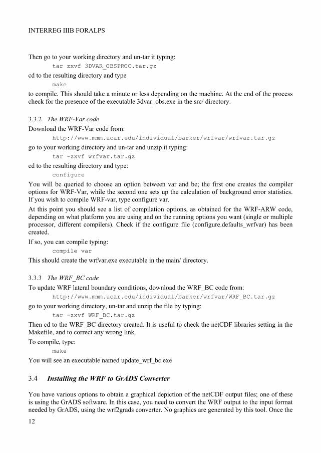
Then go to your working directory and un-tar it typing: tar zxvf 3DVAR_OBSPROC.tar.gz

cd to the resulting directory and type make

to compile. This should take a minute or less depending on the machine. At the end of the process check for the presence of the executable 3dvar_obs.exe in the src/ directory.

3.3.2 The WRF-Var code Download the WRF-Var code from:

http://www.mmm.ucar.edu/individual/barker/wrfvar/wrfvar.tar.gz

go to your working directory and un-tar and unzip it typing: tar -zxvf wrfvar.tar.gz

cd to the resulting directory and type: configure

You will be queried to choose an option between var and be; the first one creates the compiler options for WRF-Var, while the second one sets up the calculation of background error statistics. If you wish to compile WRF-var, type configure var. At this point you should see a list of compilation options, as obtained for the WRF-ARW code, depending on what platform you are using and on the running options you want (single or multiple processor, different compilers). Check if the configure file (configure.defaults_wrfvar) has been created. If so, you can compile typing:

compile var

This should create the wrfvar.exe executable in the main/ directory.

3.3.3 The WRF_BC code To update WRF lateral boundary conditions, download the WRF_BC code from:

http://www.mmm.ucar.edu/individual/barker/wrfvar/WRF_BC.tar.gz

go to your working directory, un-tar and unzip the file by typing: tar -zxvf WRF_BC.tar.gz

Then cd to the WRF_BC directory created. It is useful to check the netCDF libraries setting in the Makefile, and to correct any wrong link. To compile, type:

make

You will see an executable named update_wrf_bc.exe

3.4 Installing the WRF to GrADS Converter

You have various options to obtain a graphical depiction of the netCDF output files; one of these is using the GrADS software. In this case, you need to convert the WRF output to the input format needed by GrADS, using the wrf2grads converter. No graphics are generated by this tool. Once the

12

Technical Reports

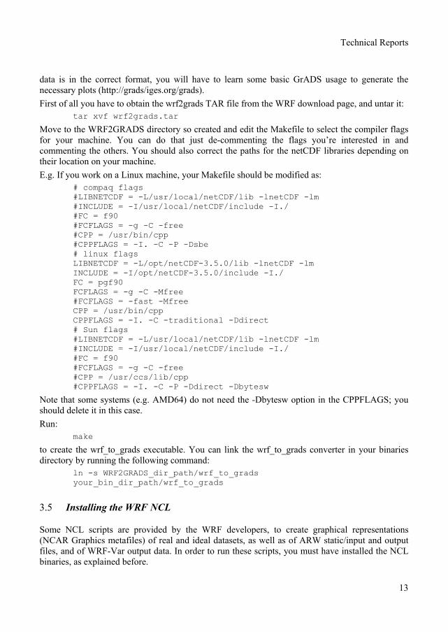
data is in the correct format, you will have to learn some basic GrADS usage to generate the necessary plots (http://grads/iges.org/grads). First of all you have to obtain the wrf2grads TAR file from the WRF download page, and untar it:

tar xvf wrf2grads.tar

Move to the WRF2GRADS directory so created and edit the Makefile to select the compiler flags for your machine. You can do that just de-commenting the flags you’re interested in and commenting the others. You should also correct the paths for the netCDF libraries depending on their location on your machine. E.g. If you work on a Linux machine, your Makefile should be modified as:

# compaq flags #LIBNETCDF = -L/usr/local/netCDF/lib -lnetCDF -lm #INCLUDE = -I/usr/local/netCDF/include -I./ #FC = f90 #FCFLAGS = -g -C -free #CPP = /usr/bin/cpp #CPPFLAGS = -I. -C -P -Dsbe # linux flags LIBNETCDF = -L/opt/netCDF-3.5.0/lib -lnetCDF -lm INCLUDE = -I/opt/netCDF-3.5.0/include -I./ FC = pgf90 FCFLAGS = -g -C -Mfree #FCFLAGS = -fast -Mfree CPP = /usr/bin/cpp CPPFLAGS = -I. -C -traditional -Ddirect # Sun flags #LIBNETCDF = -L/usr/local/netCDF/lib -lnetCDF -lm #INCLUDE = -I/usr/local/netCDF/include -I./ #FC = f90 #FCFLAGS = -g -C -free #CPP = /usr/ccs/lib/cpp #CPPFLAGS = -I. -C -P -Ddirect -Dbytesw

Note that some systems (e.g. AMD64) do not need the -Dbytesw option in the CPPFLAGS; you should delete it in this case. Run:

make

to create the wrf_to_grads executable. You can link the wrf_to_grads converter in your binaries directory by running the following command:

ln -s WRF2GRADS_dir_path/wrf_to_grads your_bin_dir_path/wrf_to_grads

3.5 Installing the WRF NCL

Some NCL scripts are provided by the WRF developers, to create graphical representations (NCAR Graphics metafiles) of real and ideal datasets, as well as of ARW static/input and output files, and of WRF-Var output data. In order to run these scripts, you must have installed the NCL binaries, as explained before.

13


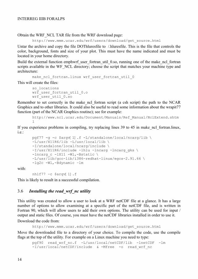
Obtain the WRF_NCL TAR file from the WRF download page: http://www.mmm.ucar.edu/wrf/users/download/get_source.html

Untar the archive and copy the file DOThluresfile to /.hluresfile. This is the file that controls the color, background, fonts and size of your plot. This must have the name indicated and must be located in your home directory. Build the external function emphwrf_user_fortran_util_0.so, running one of the make_ncl_fortran scripts available in the WF_NCL directory; choose the script that matches your machine type and architecture:

make_ncl_fortran.linux wrf_user_fortran_util_0

This will create the files: so_locations wrf_user_fortran_util_0.o wrf_user_util_0.so

Remember to set correctly in the make_ncl_fortran script (a csh script) the path to the NCAR Graphics and to other libraries. It could also be useful to read some information about the wrapit77 function (part of the NCAR Graphics routine); see for example:

http://www.ncl.ucar.edu/Document/Manuals/Ref_Manual/NclExtend.shtml

If you experience problems in compiling, try replacing lines 39 to 45 in make_ncl_fortran.linux, i.e.:

pgf77 -g -c $argv[1].f -L/standalone/local/ncarg/lib \ -L/usr/X11R6/lib -L/usr/local/lib \ -I/standalone/local/ncarg/include \ -I/usr/X11R6/include -lhlu -lncarg -lncarg_gks \ -lncarg_c -lX11 -Wl,-Bstatic \ -L/usr/lib/gcc-lib/i386-redhat-linux/egcs-2.91.66 \ -lg2c -Wl,-Bdynamic –lm

with: nhlf77 -c $argv[1].f

This is likely to result in a successful compilation.

3.6 Installing the read_wrf_nc utility

This utility was created to allow a user to look at a WRF netCDF file at a glance. It has a large number of options to allow examining at a specific part of the netCDF file, and is written in Fortran 90, which will allow users to add their own options. The utility can be used for input / output and static files. Of course, you must have the netCDF libraries installed in order to use it. Download the code from:

http://www.mmm.ucar.edu/wrf/users/download/get_source.html

Move the downloaded file to a directory of your choice. To compile the code, use the compile flags at the top of the utility. For example on a Linux machine you need to type:

pgf90 read_wrf_nc.f -L/usr/local/netCDF/lib -lnetCDF -lm -I/usr/local/netCDF/include & -Mfree -o read_wrf_nc

14

Technical Reports

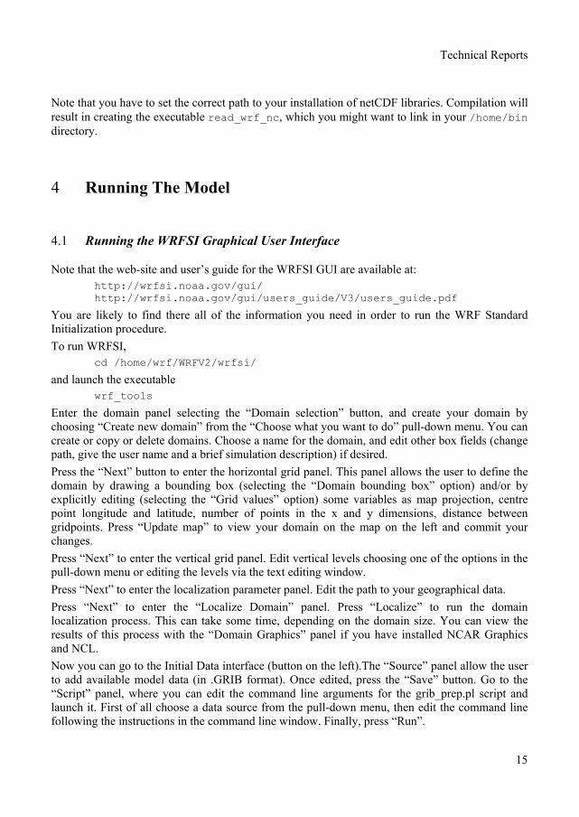
Note that you have to set the correct path to your installation of netCDF libraries. Compilation will result in creating the executable read_wrf_nc, which you might want to link in your /home/bin directory.

4 Running The Model

4.1 Running the WRFSI Graphical User Interface

Note that the web-site and user’s guide for the WRFSI GUI are available at: http://wrfsi.noaa.gov/gui/ http://wrfsi.noaa.gov/gui/users_guide/V3/users_guide.pdf

You are likely to find there all of the information you need in order to run the WRF Standard Initialization procedure. To run WRFSI,

cd /home/wrf/WRFV2/wrfsi/

and launch the executable wrf_tools

Enter the domain panel selecting the “Domain selection” button, and create your domain by choosing “Create new domain” from the “Choose what you want to do” pull-down menu. You can create or copy or delete domains. Choose a name for the domain, and edit other box fields (change path, give the user name and a brief simulation description) if desired. Press the “Next” button to enter the horizontal grid panel. This panel allows the user to define the domain by drawing a bounding box (selecting the “Domain bounding box” option) and/or by explicitly editing (selecting the “Grid values” option) some variables as map projection, centre point longitude and latitude, number of points in the x and y dimensions, distance between gridpoints. Press “Update map” to view your domain on the map on the left and commit your changes. Press “Next” to enter the vertical grid panel. Edit vertical levels choosing one of the options in the pull-down menu or editing the levels via the text editing window. Press “Next” to enter the localization parameter panel. Edit the path to your geographical data. Press “Next” to enter the “Localize Domain” panel. Press “Localize” to run the domain localization process. This can take some time, depending on the domain size. You can view the results of this process with the “Domain Graphics” panel if you have installed NCAR Graphics and NCL. Now you can go to the Initial Data interface (button on the left).The “Source” panel allow the user to add available model data (in .GRIB format). Once edited, press the “Save” button. Go to the “Script” panel, where you can edit the command line arguments for the grib_prep.pl script and launch it. First of all choose a data source from the pull-down menu, then edit the command line following the instructions in the command line window. Finally, press “Run”.

15


Once the program stops running, go to the “Interpolate Data” interface. This operation provides initial and boundary conditions running the wrfprep.pl program. In the “Control” panel you can edit the parameters needed for the interpolation. Go to the “Script” panel to edit the command line arguments, following the help in the command line options window. Press “Run”. At the end of the run, upon success you will have some files in the directory wrfsi/domains/your_domain/siprd/, named as:

wrf_real_input_d01_yyyy_mm_dd_hh:00:00

Copy or link these files in the directory where you will run the wrf model: cp wrf_real_input_d01* /home/WRFV2/test/em_real/

4.2 Running the WRF model

To run the WRF model, go to the WRFV2/ directory: cd /home/WRFV2

Compile em_real and move to the appropriate directory, i.e. the one where you have wrf_real_input_files and the two executable real.exe and wrf.exe cd test/em_real. Edit the namelist.input file with the same domain parameters you have selected by means of the WRFSI. You can find them listed in the wrfsi.nl namelist file, in the directory wrfsi/domains/your_domain/static/. Remember setting the forecast time, the number of grid points and vertical levels, the spatial resolution, the integration time step (as a rule of thumb, this should be about 6 times the spatial resolution in km, due to a combination of numerical stability criteria). The namelist.input file is also used to modify the settings of physical parameterizations. You can find all the relevant information in the README.namelist. Run the real.exe program:

real.exe

When real.exe is succesfully terminated run the model: wrf.exe

or wrf.exe >& wrf.log &

Once your run is finished you will have one or more output files named as wrf_output_date.

4.3 Running the WRF 3d-Var system

4.3.1 The 3D-Var observation preprocessor Edit the namelist.3dvar_obs in the 3DVAR_OBSPROC directory. You should read the README.namelist for details, and keep in mind that some default namelists can be used as an example. For instance, the namelist.3dvar_obs.wrfvar-tut can be used for the test data provided with the program:

cp namelist.3dvar_obs.wrfvar-tut namelist.3dvar_obs

Then you should edit the full path to observation file (ob.little_r), the grid dimensions (test data nestix=nestjx=45) and the grid resolution (dis=200km).

16

Technical Reports

Now you can run the program typing: 3dvar_obs.exe >& 3dvar_obs.out

If the program ends normally you should have an observation data file obs_gts.3dvar wich can be used as input to WRF-Var. A dedicated routine allows to have a look at the data distribution for each type of observation. Type:

cd MAP_plot

then modify the shell script Map.csh to set the time window and the full path of input observation file just created. Then type:

Map.csh

and once the job is completed you will have a gmeta.{analysis_time} file. View it by typing: idt gmeta.yyyymmddhh

Copy the output file created in your $DAT_DIR directory (the directory where you stored your observational data):

mv obs_gts.3dvar $DAT_DIR/obs_gts.3dvar.yyyymmddhh

and clean up by typing make clean

4.3.2 The WRF-Var code Mve to the wrfvar/run/ directory, edit the namelist.3dvar file and the DA_Run_WRF-Var.csh script. Type:

A_Run_WRF-Var.csh script

This will create the wrf_3dvar_output file.

4.3.3 The WRF_BC code Move to the WRF_BC directory, edit the new_bc_csh script with correct paths to the wrf_3dvar_output file, the wrfbdy* and wrfinput* files (output from WRFSI). Run the script, which should modify the wrfbdy_d01 file. Finally, rename the 3dvar output file as wrfinput:

mv wrf_3dvar_output wrfinput_d01

4.4 Running the wrf2grads converter

Once you have obtained your model outputs you can see look at them directly with NCL graphics, or convert them for use with other graphical packages with one of the programs available. For example, this section provides the instructions to use the WRF to GrADS converter. Edit the control_file indicating the timesteps and variables to process (although the list contains all variables, those indented with a blank space will be ignored), and selecting the input files (absolute or relative paths are both accepted). Even in this case, indentation with a blank space discards the file from the list. You should also set if the case is real/ideal or static, indicating which vertical levels to interpolate. For more information, you can read the README file relative to the control_file. Now you can run the program by typing:

wrf_to_grads control_file MyOutput [-options]

17


This will create a MyOutput.ctl and a MyOutput.dat file that can be read by GrADS. You can select one of the different debugging levels available using options. If you set no option, only basic information will be written to the screen. The -v and -V flags will instead print out some (or a lot of) debug information. Now you should be able to use GrADS opening the ctl file or running some of the scripts available in the WRF2GRADS directory. Pay attention to the fact that the grads scripts presume you named your ctl files by specified names. If you have not done so, you can simply modify the GrADS script at the ’open name file’ command line. Note that when converting WRF output to GrADS format using the map background option, the location of forecast gridded data is shifted with respect to the geographical background. In particular, everything seems to be shifted to the south. You can notice this for example plotting the land-mask field with GrADS. This problem arises because wrf2grads uses constant increments in the y direction (latitude direction), while latitudes in the WRF netCDF output are not equidistant (since the grid space is defined in kilometers and not in degrees). Therefore you should modify the code eliminating the constant increment and using the latitudes specified in the netCDF file, as already made for the vertical levels. So:

cd WRF2GRADS/

There, you should edit the module_wrf_t0_grads_util.F file, by finding the following lines: write(13,'("ydef ",i4," linear ",f9.4," ",f8.4)') & ny,xlat(1,1),(abs(xlat(1,1)-xlat(nx,ny))/(ny-1))

and replacing them with: write(13,'("ydef ",i4," levels ")') ny do jtest=1, ny write(13,'(" ",f10.5)') xlat(1,jtest) enddo

4.5 Running the read_wrf_nc utility

To run the utility, type: read_wrf_nc wrf_data_file_name [-options]

Note that you can use only one option at time. Launching the program with the -h option will give you a complete description of all the available options and of their usage. A special option, the “-EditData VAR”, will allow you to change a specific field and write it back in the WRF netCDF file. This option will change your current WRF netCDF file, so take care when using it. Two important things you should have in mind using this option:

– you can change only one file at time. So if you need to have more than one field changed, you will need to run the program several times, each with a different “VAR”.

– if you have multiple times in your WRF netCDF file then all the available times for the variable selected will be changed. To prevent is from happening, use the -t option, i.e. to change only the first three times of the T2 variable: [-EditData T2 -t 1 3].

To use this option, first of all make a copy of your netCDF file. Then move it to where you installed read_wrf_nc and edit the read_wrf_nc.f file. Search the file for the subroutine user_code. At this point you will have to make your changes. Add an elseif-statement for the variable you

18

Technical Reports

want to change. You have to use either the “data_real” or the “data_in” array, where the first is meant for real data and the second for integer data. Here you can find some examples:

– If you want to change all (all time periods too) values of U to a constant 10.0 m/s, you would add the following IF_statement: elseif ( var == 'U') then data_real = 10.0

– If you want to change some of the LANDMASK data from LAND to SEA points: elseif ( var == 'LANDMASK') then data_real(10:15,20:25,1) = 0

– If you want to change all ISLTYP (this is an INTEGER field representing soil category) category 3 into category 7: elseif ( var == 'ISLTYP') then where (data_int == 3 ) data_int = 7 endwhere

After finishing the compilation, re-compile and run the program with the -EditData VAR option. You will be prompted if this is really what you want to do. Only answering yes will allow the changes to take effect.

5 Ingesting ECMWF data

5.1 Creating the Vtable

To extract and decode the appropriate data from GRIB files for the model initialization, the WRFSI program use some ASCII tables, the so called Vtables, where the variables of interest and and their proper GRIB code are listed. Since different GRIB files may have different codes for the same variable, you will need different Vtables to use GRIB files from different data providers. At the moment, WRF only provides Vtables for NAM/Eta 104, 212 grid, NAM/Eta data in AWIP format, GFS (or AVN), NCEP/NCAR reanalyses, RUC and AFWA’s AGRMET land surface model output. If you wish to add a source, simply copy one of the Vtables into another one called Vtable.NAME, where NAME is of your choice, and edit it changing codes and variables according to your needs. You will need to add an entry to grib_prep.nl that matches this name. You can find the Vtables and the gri_prep.nl file in the directory $EXT_DATAROOT/static (where $EXT_DATAROOT = /wrfsi/extdata/). In the following, you can find the Vtable created to ingest ECMWF data (both analyses and forecasts) and the changes made in the namelist file cd $EXT_DATAROOT/static/

19


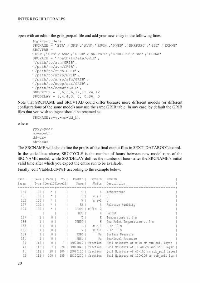
open with an editor the grib_prep.nl file and add your new entry in the following lines: &gpinput_defs SRCNAME = ’ETA’,’GFS’,’AVN’,’RUCH’,’NNRP’,’NNRPSFC’,’SST’,’ECMWF’ SRCVTAB = ’ETA’,’GFS’,’AVN’,’RUCH’,’NNRPSFC’,’NNRPSFC’,’SST’,’ECMWF’ SRCPATH = ’/path/to/eta/GRIB’, ’/path/to/avn/GRIB’, ’/path/to/avn/GRIB’, ’/path/to/ruch.GRIB’, ’/path/to/nnrp/GRIB’, ’/path/to/nnrp/sfc/GRIB’, ’/path/to/ncep/sst/GRIB’, ’/path/to/ecmwf/GRIB’, SRCCYCLE = 6,6,6,6,12,12,24,12 SRCDELAY = 3,4,4,3, 0, 0,36, 0

Note that SRCNAME and SRCVTAB could differ because more different models (or different configurations of the same model) may use the same GRIB table. In any case, by default the GRIB files that you wish to ingest should be renamed as:

SRCNAME:yyyy-mm-dd_hh

where yyyy=year mm=month dd=day hh=hour

The SRCNAME will also define the prefix of the final output files in $EXT_DATAROOT/extprd. In the code lines above, SRCCYCLE is the number of hours between new model runs of the SRCNAME model, while SRCDELAY defines the number of hours after the SRCNAME’s initial valid time after which you expect the entire run to be available. Finally, edit Vtable.ECMWF according to the example below: GRIB1 | Level| From | To | REGRID | REGRID | REGRID | Param | Type |Level1|Level2| Name | Units | Description | --------+------+------+------+----------+----------+------------------------------------------+ 130 | 100 | * | | T | K | Temperature | 131 | 100 | * | | U | m s-1 | U | 132 | 100 | * | | V | m s-1 | V | 157 | 100 | * | | RH | % | Relative Humidity | 129 | 100 | * | | GEOPT | m{2}s{-2}| | | | | | HGT | m | Height | 167 | 1 | 0 | | T | K | Temperature at 2 m | 168 | 1 | 0 | | DEWPT | K | Dew Point Temperature at 2 m | 165 | 1 | 0 | | U | m s-1 | U at 10 m | 166 | 1 | 0 | | V | m s-1 | V at 10 m | 134 | 1 | 0 | | PSFC | Pa | Surface Pressure | 151 | 1 | 0 | | PMSL | Pa | Sea-level Pressure | 39 | 112 | 0 | 7 | SM000010 | fraction | Soil Moisture of 0-10 cm sub_soil layer | 40 | 112 | 7 | 28 | SM010040 | fraction | Soil Moisture of 10-40 cm sub_soil layer | 41 | 112 | 28 | 100 | SM040100 | fraction | Soil Moisture of 40-100 cm sub_soil layer| 42 | 112 | 100 | 255 | SM100200 | fraction | Soil Moisture of 100-200 cm sub_soil lyr |

20

Technical Reports

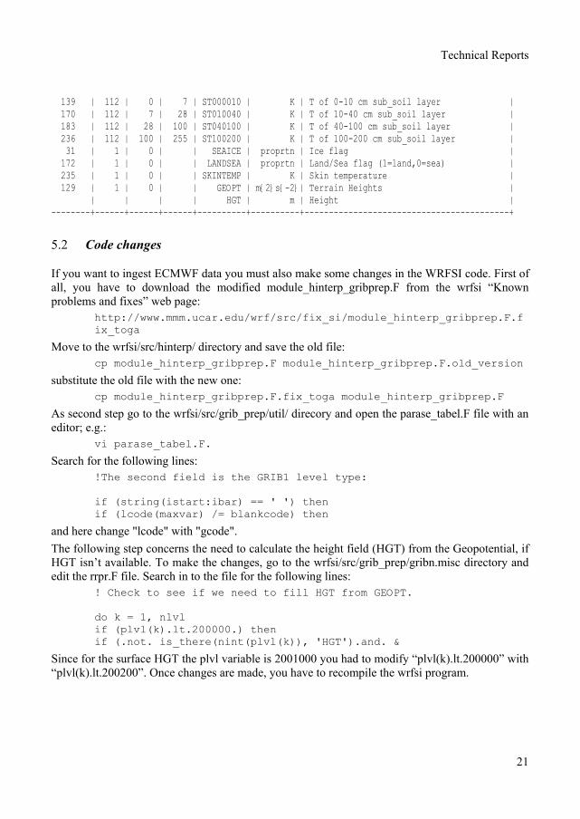
139 | 112 | 0 | 7 | ST000010 | K | T of 0-10 cm sub_soil layer | 170 | 112 | 7 | 28 | ST010040 | K | T of 10-40 cm sub_soil layer | 183 | 112 | 28 | 100 | ST040100 | K | T of 40-100 cm sub_soil layer | 236 | 112 | 100 | 255 | ST100200 | K | T of 100-200 cm sub_soil layer | 31 | 1 | 0 | | SEAICE | proprtn | Ice flag | 172 | 1 | 0 | | LANDSEA | proprtn | Land/Sea flag (1=land,0=sea) | 235 | 1 | 0 | | SKINTEMP | K | Skin temperature | 129 | 1 | 0 | | GEOPT | m{2}s{-2}| Terrain Heights | | | | | HGT | m | Height | --------+------+------+------+----------+----------+------------------------------------------+

5.2 Code changes

If you want to ingest ECMWF data you must also make some changes in the WRFSI code. First of all, you have to download the modified module_hinterp_gribprep.F from the wrfsi “Known problems and fixes” web page:

http://www.mmm.ucar.edu/wrf/src/fix_si/module_hinterp_gribprep.F.fix_toga

Move to the wrfsi/src/hinterp/ directory and save the old file: cp module_hinterp_gribprep.F module_hinterp_gribprep.F.old_version

substitute the old file with the new one: cp module_hinterp_gribprep.F.fix_toga module_hinterp_gribprep.F

As second step go to the wrfsi/src/grib_prep/util/ direcory and open the parase_tabel.F file with an editor; e.g.:

vi parase_tabel.F.

Search for the following lines: !The second field is the GRIB1 level type: if (string(istart:ibar) == ' ') then if (lcode(maxvar) /= blankcode) then

and here change "lcode" with "gcode". The following step concerns the need to calculate the height field (HGT) from the Geopotential, if HGT isn’t available. To make the changes, go to the wrfsi/src/grib_prep/gribn.misc directory and edit the rrpr.F file. Search in to the file for the following lines:

! Check to see if we need to fill HGT from GEOPT. do k = 1, nlvl if (plvl(k).lt.200000.) then if (.not. is_there(nint(plvl(k)), 'HGT').and. &

Since for the surface HGT the plvl variable is 2001000 you had to modify “plvl(k).lt.200000” with “plvl(k).lt.200200”. Once changes are made, you have to recompile the wrfsi program.

21


5.3 Possible problems

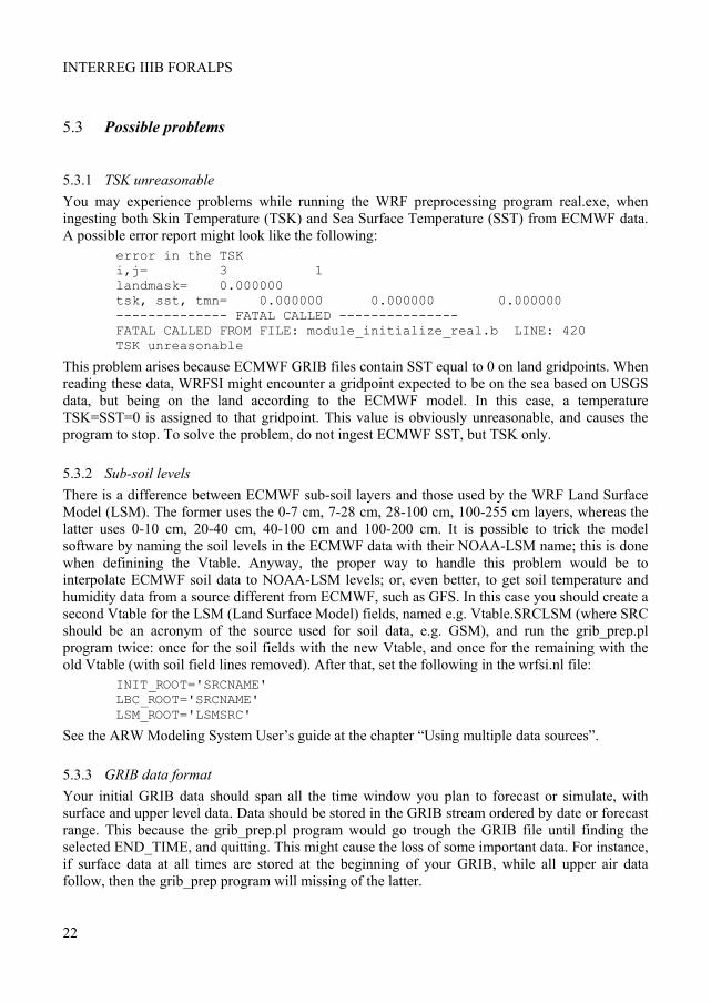
5.3.1 TSK unreasonable You may experience problems while running the WRF preprocessing program real.exe, when ingesting both Skin Temperature (TSK) and Sea Surface Temperature (SST) from ECMWF data. A possible error report might look like the following:

error in the TSK i,j= 3 1 landmask= 0.000000 tsk, sst, tmn= 0.000000 0.000000 0.000000 -------------- FATAL CALLED --------------- FATAL CALLED FROM FILE: module_initialize_real.b LINE: 420 TSK unreasonable

This problem arises because ECMWF GRIB files contain SST equal to 0 on land gridpoints. When reading these data, WRFSI might encounter a gridpoint expected to be on the sea based on USGS data, but being on the land according to the ECMWF model. In this case, a temperature TSK=SST=0 is assigned to that gridpoint. This value is obviously unreasonable, and causes the program to stop. To solve the problem, do not ingest ECMWF SST, but TSK only.

5.3.2 Sub-soil levels There is a difference between ECMWF sub-soil layers and those used by the WRF Land Surface Model (LSM). The former uses the 0-7 cm, 7-28 cm, 28-100 cm, 100-255 cm layers, whereas the latter uses 0-10 cm, 20-40 cm, 40-100 cm and 100-200 cm. It is possible to trick the model software by naming the soil levels in the ECMWF data with their NOAA-LSM name; this is done when definining the Vtable. Anyway, the proper way to handle this problem would be to interpolate ECMWF soil data to NOAA-LSM levels; or, even better, to get soil temperature and humidity data from a source different from ECMWF, such as GFS. In this case you should create a second Vtable for the LSM (Land Surface Model) fields, named e.g. Vtable.SRCLSM (where SRC should be an acronym of the source used for soil data, e.g. GSM), and run the grib_prep.pl program twice: once for the soil fields with the new Vtable, and once for the remaining with the old Vtable (with soil field lines removed). After that, set the following in the wrfsi.nl file:

INIT_ROOT='SRCNAME' LBC_ROOT='SRCNAME' LSM_ROOT='LSMSRC'

See the ARW Modeling System User’s guide at the chapter “Using multiple data sources”.

5.3.3 GRIB data format Your initial GRIB data should span all the time window you plan to forecast or simulate, with surface and upper level data. Data should be stored in the GRIB stream ordered by date or forecast range. This because the grib_prep.pl program would go trough the GRIB file until finding the selected END_TIME, and quitting. This might cause the loss of some important data. For instance, if surface data at all times are stored at the beginning of your GRIB, while all upper air data follow, then the grib_prep program will missing of the latter.

22

Technical Reports

If your data aren’t stored correctly, sort them using the wgrib program. E.g., to sort by forecast range type the following:

wgrib grib_file | sort -t: -k13,13 -n | wgrib -i grib_file -grib -o new_grib_file

Moreover, surface and upper level data should be defined in the same domain, with the same grid spacing and geographical dimensions. If not so you can reduce the larger domain using the ggrib program (currently a beta version). For instance, to reduce the domain size type:

ggrib grib_file_old grib_file_new westlon southlat eastlon northlat

If you fail obtaining surface and upper level data in the same domain, then you have to split them in two separate files, and proceed as explained at the end of the previous section: create two separate Vtables (e.g. Vtable.ECMWFSFC and Vtable.ECMWFUPL), and run the grib_prep.pl program twice, once for the surface and once for the upper levels. You will have to set the surface SRCNAME (e.g. ECMWFSFC) as LSM_ROOT as eplained in the ARW Modeling System User’s guide chapter “Using multiple data sources”.

6 References

Klemp, J. B., W. C. Skamarock, and J. Dudhia, 2007: Conservative split-explicit time integration methods for the compressible nonhydrostatic equations. Mon. Wea. Rev., 135, 20-36. Michalakes, J., J. Dudhia, D. Gill, T. Henderson, J. Klemp, W. Skamarock, and W. Wang: The Weather Research and Forecast Model: Software Architecture and Performance. Proceedings of the Eleventh ECMWF Workshop on the Use of High Performance Computing in Meteorology. Eds. Walter Zwieflhofer and George Mozdzynski. World Scientific, 2005, pp 156 – 168 Michalakes, J., S. Chen, J. Dudhia, L. Hart, J. Klemp, J. Middlecoff, and W. Skamarock: Development of a Next Generation Regional Weather Research and Forecast Model. Developments in Teracomputing: Proceedings of the Ninth ECMWF Workshop on the Use of High Performance Computing in Meteorology. Eds. Walter Zwieflhofer and Norbert Kreitz. World Scientific, 2001, pp. 269-276. Skamarock, W. C., 2004: Evaluating Mesoscale NWP Models Using Kinetic Energy Spectra. Mon. Wea., Rev., 132, 3019-3032 Skamarock, W. C., J. B. Klemp, J. Dudhia, D. O. Gill, D. M. Barker, W. Wang, and J. G. Powers, 2005: A description of the Advanced Research WRF Version 2. NCAR Tech Notes-468+STR Skamarock, W. C., 2006: Positive-Definite and Montonic Limiters for Unrestricted-Timestep Transport Schemes. Mon. Wea. Rev., 134, 2241-2250 Skamarock, W. C., and J. B. Klemp, 2007: A time-split nonhydrostatic atmospheric model for research and NWP applications. J. Comp. Phys., accepted. Wicker, L. J., and W. C. Skamarock, 2002: Time splitting methods for elastic models using forward time schemes. Mon. Wea. Rev., 130, 2088-2097. User’s Guide for Advanced Research WRF (ARW), Modeling System Version 2.1 (October 2005) WRF Users web page: http://www.mmm.ucar.edu/wrf/users/

23

http://www.mmm.ucar.edu/wrf/users/


NOTES

24

UniTN

(Lead partner)

University of Trento

Department of Civil and Environmental Engineering www.ing.unitn.it

APAT

Italian Agency for Environmental Protection

and Technical Services www.apat.gov.it

ARPALombardia

Regional Agency for Environmental Protection

Lombardia

Meteorological Service-Hydrographic Offi ce www.arpalombardia.it

ARPAV


Veneto www.arpa.veneto.it

EARS

Environmental Agency of the

Republic of Slovenia www.arso.gov.si

OSMER


Friuli-Venezia Giulia

Regional Meteorological Observatory www.osmer.fvg.it

PAB

Autonomous Province of Bolzano

Hydrographic Offi ce www.provincia.bz.it

PAT

Autonomous Province of Trento

Offi ce for Forecasts and Organization www.meteotrentino.it

RAVA

Valle d’Aosta Autonomous Region

Meteorological Offi ce www.regione.vda.it

ZAMG-I

Central Institute for Meteorology and Geodynamics:

Regional Offi ce for Tirol and Vorarlberg

www.zamg.ac.at

ZAMG-K


Regional Offi ce for Carinthia

ZAMG-S


Regional Offi ce for Salzburg and Oberösterreich

ZAMG-W


Regional Offi ce for Wien, Niederösterreich and Burgenland

Foralps Partnership

ISBN 978–88–8443–232–2

abcdefghijk

The project FORALPS pursued improvements in the knowledge of weather and climate processes in the Alps, required for a more sustainable management of their water resources. The FORALPS Technical Reports series presents the original achievements of the project, and provides an accessible introduction to selected topics in hydro-meteorological monitoring and analysis.

www.foralps.net

Documents

A GUIDE TO THE WRF NUMERICAL WEATHER · PDF fileA guide to the WRF numerical weather prediction model Irene GALLAI Regional Agency for Environmental Protection of Friuli Venezia Giulia