A high order ENO conservative Lagrangian scheme for the

compressible Euler equations

Juan Cheng1 and Chi-Wang Shu2

Abstract

We develop a class of Lagrangian schemes for solving the Euler equations of compressible

gas dynamics both in the Cartesian and in the cylindrical coordinates. The schemes are

based on high order essentially non-oscillatory (ENO) reconstruction. They are conservative

for the density, momentum and total energy, can maintain formal high order accuracy both

in space and time and can achieve at least uniformly second order accuracy with moving

and distorted Lagrangian meshes, are essentially non-oscillatory, and have no parameters

to be tuned for individual test cases. One and two dimensional numerical examples in the

Cartesian and cylindrical coordinates are presented to demonstrate the performance of the

schemes in terms of accuracy, resolution for discontinuities, and non-oscillatory properties.

Keywords: Lagrangian scheme; high order accuracy; conservative scheme; ENO recon-

struction; compressible Euler equations; ALE method

1Institute of Applied Physics and Computational Mathematics, Beijing 100088, China. E-mail:cheng juan@iapcm.ac.cn. Research is supported in part by NSFC grant 10572028. Additional support isprovided by the National Basic Research Program of China under grant 2005CB321702, by the Foundationof National Key Laboratory of Computational Physics under grant 9140C6902010603 and by the NationalHi-Tech Inertial Confinement Fusion Committee of China.

2Division of Applied Mathematics, Brown University, Providence, RI 02912. E-mail:shu@dam.brown.edu. Research is supported in part by NSFC grant 10671190 and by the ChineseAcademy of Sciences during his visit to the University of Science and Technology of China and the Instituteof Computational Mathematics and Scientific / Engineering Computing. Additional support is provided byARO grant W911NF-04-1-0291 and NSF grant DMS-0510345.

1

1 Introduction

In numerical simulations of multidimensional fluid flow, there are two typical choices: a

Lagrangian framework, in which the mesh moves with the local fluid velocity, and an Eulerian

framework, in which the fluid flows through a grid fixed in space. More generally, the motion

of the grid can also be chosen arbitrarily, this method is called the Arbitrary Lagrangian-

Eulerian method (ALE; cf. [14, 3, 20, 16, 23]). Most ALE algorithms consist of three phases,

a Lagrangian phase in which the solution and the grid are updated, a rezoning phase in which

the nodes of the computational grid are moved to a more optimal position and a remapping

phase in which the Lagrangian solution is transferred to the new grid.

In this paper, we focus on computational hydrodynamic methods for the Euler equations

where the mesh moves with the flow velocity. Such methods, therefore, imply the use of

distorted or nonuniform meshes. Particular examples include the Lagrangian methods, or

the ALE methods which contain a Lagrangian phase.

Lagrangian methods are widely used in many fields for multi-material flow simulations

such as astrophysics and computational fluid dynamics (CFD), due to their distinguished

advantage of being able to capture the material interface sharply. Comparing with Eulerian

methods, Lagrangian methods avoid a source of numerical error due to the advection terms

in the conservation equations. For this reason, Lagrangian methods are frequently preferred

in one-dimensional computations where mesh distortion plays no role. Even though the

Euler equations are much simpler in the Lagrangian framework as they do not contain the

advection terms, in two or more space dimensions they are actually more difficult to solve

since the mesh moves with the fluid and can easily lose its quality. In the past years, many

efforts have been made to develop Lagrangian methods. Some algorithms are developed

from the nonconservative form of the Euler equations, for example, those discussed in [21,

4, 5, 6, 18, 35]. The other class of Lagrangian algorithms starts from the conservative form

of the Euler equations which usually can guarantee exact conservation. See for example

[3, 9, 8, 17, 32, 2] etc.

2

Most existing Lagrangian schemes for the Euler equations have first or at most second

order accuracy. Among them many Lagrangian schemes of non conservative form are only

first order accurate because of a first order error due to the nonconservative formulation of

the momentum equation. On the other hand, some of the conservative Lagrangian schemes

apply the linear interpolation strategy to achieve second order accuracy, meanwhile they

usually use a flux limiter to control spurious oscillations which leads to a possible loss of this

second order accuracy at some special points such as smooth extrema and sonic points.

Essentially non-oscillatory (ENO) schemes, first introduced by Harten and Osher [13]

and Harten et al. [12], can achieve uniformly high-order accuracy with sharp, essentially

non-oscillatory shock transitions. In the subsequent years, ENO schemes in the Eulerian

formulation have accomplished successful applications in many fields especially with prob-

lems containing both shocks and complicated smooth flow structures, see for example [27].

Eulerian ENO schemes on unstructured meshes are developed in [1]. However, the applica-

tion of the ENO methodology in the Lagrangian formulation does not seem to have been

extensively explored.

In this paper, we develop a class of Lagrangian schemes for solving the Euler equations

which are based on the high order ENO reconstruction both in the Cartesian and in the

cylindrical coordinates. The schemes are conservative for the density, momentum and total

energy, can maintain formal high order accuracy both in space and time and can achieve

at least uniformly second order accuracy on moving and distorted Lagrangian meshes, are

essentially non-oscillatory, and have no parameters to be tuned for individual test cases. They

can also be extended to higher than second order accuracy by using curved meshes. Several

one and two dimensional numerical examples in the Cartesian and cylindrical coordinates are

presented which demonstrate the good performance of the schemes both in purely Lagrangian

and in ALE calculations.

An outline of the rest of this paper is as follows. In Section 2, we describe the individual

steps of the ENO Lagrangian scheme in one space dimension. In Section 3, we present one

3

dimensional numerical results. In Section 4, we extend the scheme to two space dimensions

both in the Cartesian and in the cylindrical coordinates, while in Section 5 two dimensional

numerical examples are given to verify the performance of the ENO Lagrangian method. In

Section 6 we will give concluding remarks.

2 High order ENO conservative Lagrangian scheme –one space dimension

2.1 The compressible Euler equations in Lagrangian formulation

The Euler equations for unsteady compressible flow in the reference frame of a moving control

volume can be expressed in integral form in the Cartesian coordinates as

d

dt

!

Ω(t)

UdΩ+

!

Γ(t)

FdΓ = 0 (2.1)

where Ω(t) is the moving control volume enclosed by its boundary Γ(t). The vector of the

conserved variables U and the flux vector F are given by

U =

"

#ρME

$

% , F =

"

#(u − x) · nρ

(u− x) · nM + p · n(u− x) · nE + pu · n

$

% (2.2)

where ρ is the density, u is the velocity, M = ρu is the momentum, E is the total energy and

p is the pressure, x is the velocity of the control volume boundary Γ(t), n denotes the unit

outward normal to Γ(t). The system (2.1) represents the conservation of mass, momentum

and energy.

The set of equations is completed by the addition of an equation of state (EOS) with the

following general form

p = p(ρ, e) (2.3)

where e = E! − 1

2 |u|2 is the specific internal energy. Especially, if we consider the ideal gas,

then the equation of state has a simpler form,

p = (γ − 1)ρe

4

where γ is a constant representing the ratio of specific heat capacities of the fluid.

This paper focuses on solving the governing equations (2.1)-(2.2) in a Lagrangian frame-

work, in which it is assumed that x = u, and the vectors U and F then take the simpler

form

U =

"

#ρME

$

% , F =

"

#0

p · npu · n

$

% . (2.4)

2.2 The ENO conservative Lagrangian scheme in one space di-mension

Here we develop a conservative Lagrangian finite volume scheme both on the staggered mesh

and on the non-staggered mesh. We solve the conserved variables such as density, momentum

and total energy directly. The non-staggered mesh means that all the conserved variables,

in the form of cell averages, are stored at the cell’s center and this cell is their common

control volume. The staggered mesh implies that there are two sets of control volumes for

the considered conserved variables, i.e., the density and total energy are cell-centered and

their control volume is the cell they are located in, while the momentum is vertex-centered

which uses a different control volume (also called a dual cell). We consider two types of dual

cells on the staggered mesh, one is the domain surrounded by its two neighboring nodes,

the other is the domain surrounded by the centers of its two neighboring cells. Since the

discretization steps are similar, for simplicity, we only show the scheme on the second kind

of the staggered mesh.

The spatial domain Ω is discretized into N computational cells Ii+1/2 = [xi, xi+1] of sizes

∆xi+1/2 = xi+1 − xi with i = 1, . . . , N . For a given cell Ii+1/2, the location of the cell center

is denoted by xi+1/2. The fluid velocity ui is defined at the vertex of the mesh. On the

non-staggered mesh, all variables except the velocity are stored at the cell center xi+1/2 in

the form of cell averages. For example, the values of the cell averages for Cell Ii+1/2, denoted

by ρi+1/2, M i+1/2 and Ei+1/2, are defined as follows

ρi+1/2 =1

∆xi+1/2

!

Ii+1/2

ρdx, M i+1/2 =1

∆xi+1/2

!

Ii+1/2

Mdx, Ei+1/2 =1

∆xi+1/2

!

Ii+1/2

Edx.

5

On the staggered mesh, the difference from the non-staggered mesh is that the momentum

M i is stored at the vertex xi and its control volume is Ii = [xi−1/2, xi+1/2] which is of the

size ∆xi = xi+1/2 − xi−1/2. Thus

ρi+1/2 =1

∆xi+1/2

!

Ii+1/2

ρdx, M i =1

∆xi

!

Ii

Mdx, Ei+1/2 =1

∆xi+1/2

!

Ii+1/2

Edx.

2.2.1 Spatial discretization

We first formulate the semi-discrete finite volume scheme of the governing equations (2.1)

and (2.4) on the non-staggered mesh as

d

dt

"

#ρi+1/2∆xi+1/2

M i+1/2∆xi+1/2

Ei+1/2∆xi+1/2

$

% = −

"

#fD(U−

i+1,U+i+1) − fD(U−

i ,U+i )

fM(U−i+1,U

+i+1) − fM(U−

i ,U+i )

fE(U−i+1,U

+i+1) − fE(U−

i ,U+i )

$

% (2.5)

where fD is the numerical flux of mass across the boundary of its control volume Ii+1/2(t),

which is consistent with the physical flux (2.4) in the sense that fD(U,U) = 0, fM is the

numerical flux of momentum with fM(U,U) = p, and fE is the numerical flux of total

energy with fE(U,U) = pu. U±i and U±

i+1 represent the left and right values of U at the

cell’s boundary xi and xi+1 respectively.

The conservative semi-discrete scheme has the following form on the staggered mesh

d

dt

"

#ρi+1/2∆xi+1/2

M i∆xi

Ei+1/2∆xi+1/2

$

% = −

"

&#fD(U−

i+1,U+i+1) − fD(U−

i ,U+i )

fM(U−i+1/2,U

+i+1/2) − fM(U−

i−1/2,U+i−1/2)

fE(U−i+1,U

+i+1) − fE(U−

i ,U+i )

$

'% . (2.6)

Since the method to determine the flux at the boundary of the control volume for the

above two sets of meshes are similar, in the following we only describe the procedure on the

non-staggered mesh.

The first step for establishing the scheme is to determine the fluxes (fD, fM , fE), and the

first stage of this step is to identify the values of the primitive variables on each side of the

boundary, that is U±i , i = 1, . . . , N . The information we have is the cell average values of

the conserved variables Ui+1/2 = (ρi+1/2, M i+1/2, Ei+1/2), thus we will have to reconstruct

these variables. The simplest reconstruction is to assume that all the variables are piecewise

6

constant, and equal to the given cell averages for each cell. Then we will have ρ−i = ρi−1/2,

ρ+i = ρi+1/2 etc., where ρ−i and ρ+

i are the values of density at the left side and the right side

of the cell’s boundary xi. This reconstruction is very simple, but is only first-order accurate.

To obtain uniformly second or higher order accurate schemes, in this paper we will use the

ENO idea [12] to reconstruct polynomial functions on each Ii+1/2 by using the information

of the cell Ii+1/2 and its neighbors, such that they are second or higher order accurate

approximations to the functions ρ(x), M(x) and E(x) etc. on Ii+1/2. The procedure allows

us to obtain arbitrary high order accurate approximation by a proper reconstruction. For

simplicity, in this paper we will only discuss second and third order accurate schemes by

performing the second and third order accurate reconstructions. It is easy to extend the

procedure to a higher order reconstruction.

The method of local characteristic decomposition is used in the procedure of the ENO

reconstruction. We refer to [31] for the details of the Roe-type characteristic decomposition

that we have used in this paper. As to the details of how to conservatively reconstruct a

polynomial by the ENO idea in each cell, we refer to [12]. The approximate values of each

conserved variable at both sides of the cell’s boundary are obtained from its reconstructed

polynomial. Finally we obtain the values of the density ρ−i , ρ+i , the momentum M−

i , M+i

and the total energy E−i , E+

i at the left side and the right side of the cell’s boundary xi

respectively.

Next, we will compute the fluxes given the primitive states at each side of a control

volume’s boundary.

In this paper we use the following three typical numerical fluxes:

1) The Godunov flux,

2) The L-F (Lax-Friedrichs) flux,

3) The HLLC (Harten-Lax-van Leer contact wave) flux.

The above three approximate fluxes have been originally developed for solving compress-

ible Euler equations in the Eulerian formulation. Although these fluxes have been very

7

successful in the Eulerian formulation, their accuracy and robustness for solving the Euler

equations in an Lagrangian framework are less explored.

In the following, we will describe the implementation of these three fluxes in our La-

grangian schemes.

1. The Godunov flux

To solve the exact Riemann problem at the cell’s boundary xi, we need to know the

left and right states at the boundary. We would like to note that in a Lagrangian

scheme the velocity at each side of xi used here should be the relative fluid velocity,

that is, u−i − xi and u+

i − xi, where u−i = M−

i /ρ−i , u+i = M+

i /ρ+i and xi is the cell

boundary’s moving velocity which can be numerically determined as the Roe average√

!−i u−i +

√!+

i u+i√

!−i +√

!+i

. The pressure values at the two sides of the vertex xi are of the form

p−i = (γ − 1)[E−i − 1

2(M−i )2/ρ−i ], p+

i = (γ − 1)[E+i − 1

2(M+i )2/ρ+

i ] if the ideal gas is

considered. With the left state ρ−i , u−i − xi, p

−i and the right state ρ+

i , u+i − xi, p

+i at

xi, we can now obtain the pressure p∗i and the relative velocity u′i at xi by the Riemann

solver. The absolute velocity u∗i at xi should be u

′i + xi. Thus the fluxes fD, fM and

fE in Scheme (2.5) have the following form

()

*

fD(U−i ,U+

i ) = 0fM(U−

i ,U+i ) = p∗i

fE(U−i ,U+

i ) = p∗i u∗i .

(2.7)

2. The L-F (Lax-Friedrichs) flux

The Lax-Friedrichs flux with the simple form is given by

()

*

fD(U−i ,U+

i ) = 12 [0 − αi(ρ

+i − ρ−i )]

fM(U−i ,U+

i ) = 12 [(p

−i + p+

i ) − αi(M+i − M−

i )]fE(U−

i ,U+i ) = 1

2 [(p−i u−

i + p+i u+

i ) − αi(E+i − E−

i )]

(2.8)

where αi is taken as an upper bound for the eigenvalues of the Jacobian, here in the

Lagrangian formulation, αi = max(c−i , c+i ), where c±i are the left and right values of

the sound speed at xi. In order to reduce the numerical viscosity, we perform the local

8

characteristic decomposition and then choose a different αi for each characteristic field

based on the size of the corresponding eigenvalue, rather than using the same αi for

all components as in (2.8).

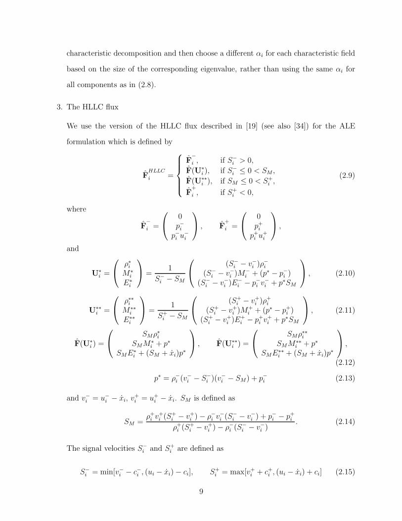
3. The HLLC flux

We use the version of the HLLC flux described in [19] (see also [34]) for the ALE

formulation which is defined by

FHLLC

i =

(+++)

+++*

F−i , if S−

i > 0,F(U∗

i ), if S−i ≤ 0 < SM ,

F(U∗∗i ), if SM ≤ 0 < S+

i ,

F+

i , if S+i < 0,

(2.9)

where

F−i =

"

#0p−i

p−i u−i

$

% , F+

i =

"

#0p+

i

p+i u+

i

$

% ,

and

U∗i =

"

#ρ∗iM∗

i

E∗i

$

% =1

S−i − SM

"

#(S−

i − v−i )ρ−i

(S−i − v−

i )M−i + (p∗ − p−i )

(S−i − v−

i )E−i − p−i v−

i + p∗SM

$

% , (2.10)

U∗∗i =

"

#ρ∗∗iM∗∗

i

E∗∗i

$

% =1

S+i − SM

"

#(S+

i − v+i )ρ+

i

(S+i − v+

i )M+i + (p∗ − p+

i )(S+

i − v+i )E+

i − p+i v+

i + p∗SM

$

% , (2.11)

F(U∗i ) =

"

#SMρ∗i

SMM∗i + p∗

SME∗i + (SM + xi)p∗

$

% , F(U∗∗i ) =

"

#SMρ∗∗i

SMM∗∗i + p∗

SME∗∗i + (SM + xi)p∗

$

% ,

(2.12)

p∗ = ρ−i (v−i − S−

i )(v−i − SM) + p−i (2.13)

and v−i = u−

i − xi, v+i = u+

i − xi. SM is defined as

SM =ρ+

i v+i (S+

i − v+i ) − ρ−i v−

i (S−i − v−

i ) + p−i − p+i

ρ+i (S+

i − v+i ) − ρ−i (S−

i − v−i )

. (2.14)

The signal velocities S−i and S+

i are defined as

S−i = min[v−

i − c−i , (ui − xi) − ci], S+i = max[v+

i + c+i , (ui − xi) + ci] (2.15)

9

where ui and ci are the Roe’s average variables for the velocity and the speed of sound.

Since we are considering the Euler equations in the Lagrangian formulation, here we

have xi = ui.

Each of the above approximate fluxes has its own special features. The Godunov flux

solves exactly the Riemann problem at the cell boundary and thus it has the least numerical

viscosity among all the first order upwind fluxes. In particular, it has no numerical viscosity

for the first equation hence it can maintain the mass of each cell unchanged during the

time marching. But it also has the disadvantage of high computational cost. The L-F flux

has relatively more numerical viscosity but it has a very simple form and is more robust

in applications. The HLLC flux’s viscosity and cost are between the Godunov flux and the

L-F flux. It has good performance in many applications. We remark that both the L-F

flux and the HLLC flux apply the numerical viscosity in all the equations including the

mass equation, causing a possible change in the cell mass during the time evolution. We

do, however, find in the following tests that the L-F flux and HLLC flux perform well on

capturing the contact discontinuities in our Lagrangian schemes. In the actual simulation,

especially in the ALE calculation, we can choose the most suitable flux depending on the

requirement of the individual problem.

2.2.2 The determination of the vertex velocity

In the Lagrangian formulation, the grid moves with the fluid velocity which is defined at the

vertex, thus we would need to know the velocity at the vertex to move the grid. Since the

velocity is a derived quantity, we would need to obtain it from the conserved variables. In

the following we describe how to determine the vertex’s velocity in our schemes.

For the Godunov flux, since we solve exactly the Riemann problem at each vertex as a

cell’s boundary, we naturally obtain the velocity by the Riemann solver there.

For the L-F flux and the HLLC flux, the velocity at the cell’s vertex is defined as the

10

Roe’s average of velocities from both sides,

ui =

,ρ−i u−

i +,

ρ+i u+

i,ρ−i +

,ρ+

i

. (2.16)

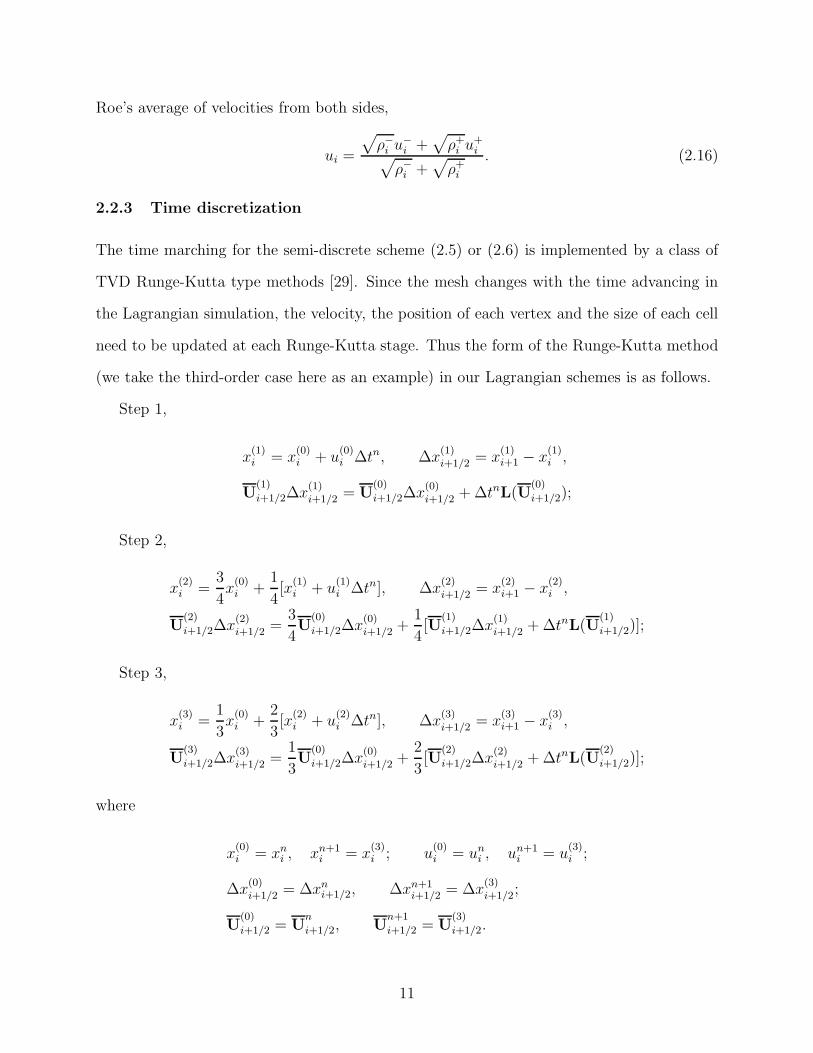
2.2.3 Time discretization

The time marching for the semi-discrete scheme (2.5) or (2.6) is implemented by a class of

TVD Runge-Kutta type methods [29]. Since the mesh changes with the time advancing in

the Lagrangian simulation, the velocity, the position of each vertex and the size of each cell

need to be updated at each Runge-Kutta stage. Thus the form of the Runge-Kutta method

(we take the third-order case here as an example) in our Lagrangian schemes is as follows.

Step 1,

x(1)i = x(0)

i + u(0)i ∆tn, ∆x(1)

i+1/2 = x(1)i+1 − x(1)

i ,

U(1)i+1/2∆x(1)

i+1/2 = U(0)i+1/2∆x(0)

i+1/2 +∆tnL(U(0)i+1/2);

Step 2,

x(2)i =

3

4x(0)

i +1

4[x(1)

i + u(1)i ∆tn], ∆x(2)

i+1/2 = x(2)i+1 − x(2)

i ,

U(2)i+1/2∆x(2)

i+1/2 =3

4U

(0)i+1/2∆x(0)

i+1/2 +1

4[U

(1)i+1/2∆x(1)

i+1/2 +∆tnL(U(1)i+1/2)];

Step 3,

x(3)i =

1

3x(0)

i +2

3[x(2)

i + u(2)i ∆tn], ∆x(3)

i+1/2 = x(3)i+1 − x(3)

i ,

U(3)i+1/2∆x(3)

i+1/2 =1

3U

(0)i+1/2∆x(0)

i+1/2 +2

3[U

(2)i+1/2∆x(2)

i+1/2 +∆tnL(U(2)i+1/2)];

where

x(0)i = xn

i , xn+1i = x(3)

i ; u(0)i = un

i , un+1i = u(3)

i ;

∆x(0)i+1/2 = ∆xn

i+1/2, ∆xn+1i+1/2 = ∆x(3)

i+1/2;

U(0)i+1/2 = U

ni+1/2, U

n+1i+1/2 = U

(3)i+1/2.

11

L is the numerical spatial operator representing the right hand of the scheme (2.5). Here

the variables with the superscripts n and n + 1 represent the values of the corresponding

variables at the n-th and (n + 1)-th time steps respectively.

Consistently with the order of the spatial discretization in the scheme (2.5), we apply

the Runge-Kutta method of the same order for its time marching.

At the end of this section, we list the explicit form of our first order Lagrangian scheme

as an example,

"

&#ρn+1

i+1/2∆xn+1i+1/2 − ρn

i+1/2∆xni+1/2

Mn+1i+1/2∆xn+1

i+1/2 − Mni+1/2∆xn

i+1/2

En+1i+1/2∆xn+1

i+1/2 − Eni+1/2∆xn

i+1/2

$

'% = −∆tn

"

#fD(Un−

i+1,Un+i+1) − fD(Un−

i ,Un+i )

fM(Un−i+1,U

n+i+1) − fM(Un−

i ,Un+i )

fE(Un−i+1,U

n+i+1) − fE(Un−

i ,Un+i )

$

%

(2.17)

where the time step ∆tn is determined as

∆tn = λ mini=1,...,N

(∆xni /cn

i )

with the Courant number λ chosen as λ = 0.6 in our computation.

3 Numerical results in one space dimension

In this section, we perform some numerical experiments in one space dimension. Purely

Lagrangian computation and the ideal gas with γ = 1.4 are used to do the following tests

unless otherwise stated. We have used the Godunov flux, the L-F flux and the HLLC flux

respectively and the results are mostly similar, so only those with the HLLC flux are listed

to save space.

3.1 Accuracy test

We first test the accuracy of our schemes on a problem with smooth solutions. The initial

condition we choose for the accuracy test is:

ρ(x, 0) = 2 + sin(2πx), u(x, 0) = 1 + 0.1 sin(2πx), p(x, 0) = 1, x ∈ [0, 1]

12

Table 3.1: Errors of the first order scheme on 1D non-staggered meshes using Nx initiallyuniform mesh cells.

Nx Norm Density order Momentum order Energy order100 L1 0.11E-1 0.15E-1 0.29E-1

L∞ 0.34E-1 0.46E-1 0.78E-1200 L1 0.55E-2 0.93 0.78E-2 0.95 0.15E-1 0.93

L∞ 0.19E-1 0.89 0.25E-1 0.86 0.42E-1 0.88400 L1 0.28E-2 0.97 0.40E-2 0.97 0.77E-2 0.96

L∞ 0.97E-2 0.93 0.13E-1 0.92 0.22E-1 0.93800 L1 0.14E-2 0.98 0.20E-2 0.98 0.39E-2 0.98

L∞ 0.50E-2 0.96 0.69E-2 0.96 0.11E-1 0.96

with a periodic boundary condition. Since we do not know the exact solution, we take the

numerical results by using the fifth order Eulerian WENO scheme [15] with 8000 grids as

the reference “exact” solution. In Tables 3.1-3.2, we summarize the errors and numerical

rate of convergence of our first and second order Lagrangian schemes at t = 1 on the 1D

non-staggered meshes. We can clearly see from Tables 3.1 and 3.2 that the first and second

order schemes achieve the designed order of accuracy, at least in the L1 norm. However, we

do observe a degeneracy of the L∞ error for the second order scheme in Table 3.2, which

is related to an accuracy degeneracy phenomenon of ENO schemes, originally discussed in

[24] for Eulerian formulated schemes. This degeneracy is more serious for the third order

scheme, hence we have used the modified third order ENO scheme via the introduction of a

biasing factor introduced in [26]. The effect of using this factor in the stencil determination

procedure is to bias towards a linearly stable stencil in smooth regions. Table 3.3 shows the

error results of the modified ENO scheme by using a factor of 2, according to the suggestion

in [26]. From this table, we can see the modified ENO scheme produces the correct third

order accuracy. The following third order non-oscillatory tests are all performed by the

modified third order ENO scheme, verifying its non-oscillatory property for problems with

discontinuities.

13

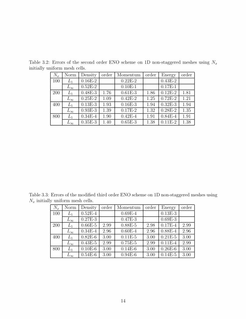
Table 3.2: Errors of the second order ENO scheme on 1D non-staggered meshes using Nx

initially uniform mesh cells.

Nx Norm Density order Momentum order Energy order100 L1 0.16E-2 0.22E-2 0.43E-2

L∞ 0.52E-2 0.10E-1 0.17E-1200 L1 0.48E-3 1.76 0.61E-3 1.86 0.12E-2 1.81

L∞ 0.25E-2 1.09 0.42E-2 1.25 0.72E-2 1.21400 L1 0.13E-3 1.93 0.16E-3 1.94 0.32E-3 1.94

L∞ 0.93E-3 1.39 0.17E-2 1.32 0.28E-2 1.35800 L1 0.34E-4 1.90 0.42E-4 1.91 0.84E-4 1.91

L∞ 0.35E-3 1.40 0.65E-3 1.38 0.11E-2 1.38

Table 3.3: Errors of the modified third order ENO scheme on 1D non-staggered meshes usingNx initially uniform mesh cells.

Nx Norm Density order Momentum order Energy order100 L1 0.52E-4 0.69E-4 0.13E-3

L∞ 0.27E-3 0.47E-3 0.69E-3200 L1 0.66E-5 2.99 0.88E-5 2.98 0.17E-4 2.99

L∞ 0.34E-4 2.96 0.60E-4 2.96 0.88E-4 2.96400 L1 0.82E-6 3.00 0.11E-5 3.00 0.21E-5 3.00

L∞ 0.43E-5 2.99 0.75E-5 2.99 0.11E-4 2.99800 L1 0.10E-6 3.00 0.14E-6 3.00 0.26E-6 3.00

L∞ 0.54E-6 3.00 0.94E-6 3.00 0.14E-5 3.00

14

3.2 Non-oscillatory tests

Example 3.1 (Lax problem). The first non-oscillatory test is the Riemann problem proposed

by Lax. Its initial condition is as follows

(ρL, uL, pL) = (0.445, 0.698, 3.528), (ρR, uR, pR) = (0.5, 0, 0.571).

Figure 3.1 shows the results with 200 initially uniform cells on the non-staggered mesh and

on the staggered mesh at t = 1.

Comparing with the exact solution, we observe satisfactory non-oscillatory results for the

non-staggered mesh in the left pictures of Figure 3.1, while there are obvious oscillations for

the staggered mesh in the right pictures of Figure 3.1. Notice that the spurious oscillations

appear even for the first order scheme, indicating that the problem is not due to the high

order reconstruction. In order to explore further the possible reason for these oscillations,

we study a simpler test case with the initial condition

ρ(x, 0) = 2 + sin(2πx), u(x, 0) = 1, p(x, 0) = 1, x ∈ [0, 1].

and a periodic boundary condition. The exact solution is easily given as

ρ(x, t) = 2 + sin(2π(x − t)), u(x, t) = 1, p(x, t) = 1.

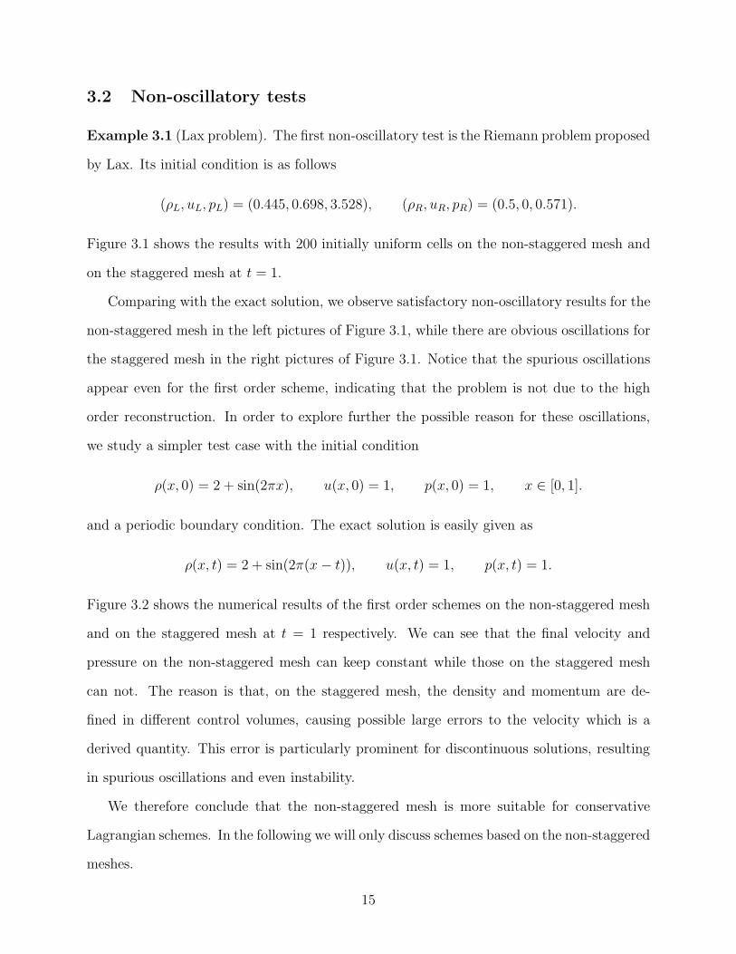
Figure 3.2 shows the numerical results of the first order schemes on the non-staggered mesh

and on the staggered mesh at t = 1 respectively. We can see that the final velocity and

pressure on the non-staggered mesh can keep constant while those on the staggered mesh

can not. The reason is that, on the staggered mesh, the density and momentum are de-

fined in different control volumes, causing possible large errors to the velocity which is a

derived quantity. This error is particularly prominent for discontinuous solutions, resulting

in spurious oscillations and even instability.

We therefore conclude that the non-staggered mesh is more suitable for conservative

Lagrangian schemes. In the following we will only discuss schemes based on the non-staggered

meshes.

15

X0 5 10 15 200

0.5

1

1.5

2

2.5

3

3.5

exact1st order

non-staggered mesh

!

u

p

X0 5 10 15 200

1

2

3exact1st order

staggered mesh

!

u

p

X0 5 10 15 200

0.5

1

1.5

2

2.5

3

3.5

exact2nd order

non-staggered mesh

!

u

p

X0 5 10 15 200

1

2

3exact2nd order

staggered mesh

!

u

p

X0 5 10 15 200

0.5

1

1.5

2

2.5

3

3.5

exact3rd order

non-staggered mesh

!

u

p

X0 5 10 15 200

1

2

3exact3rd order

staggered mesh

!

u

p

Figure 3.1: The results of the Lax problem on a 200 initially uniform cells. Left: non-staggered mesh; Right: staggered mesh. Top: first order; Middle: second order; Bottom:third order.

16

X1 1.2 1.4 1.6 1.80.8

0.85

0.9

0.95

1

1.05

1.1

1.15

1.2

1st order

non-staggered mesh

!

u

p

X1 1.2 1.4 1.6 1.8

0.85

0.9

0.95

1

1.05

1.1

1.15

1.2

1st order

staggered mesh

!

u

p

Figure 3.2: Density, velocity and pressure of the first order schemes. Left: on the non-staggered mesh; Right: on the staggered mesh.

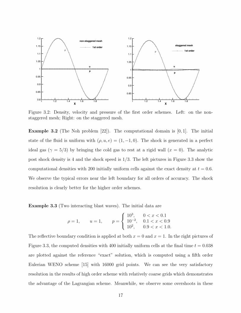
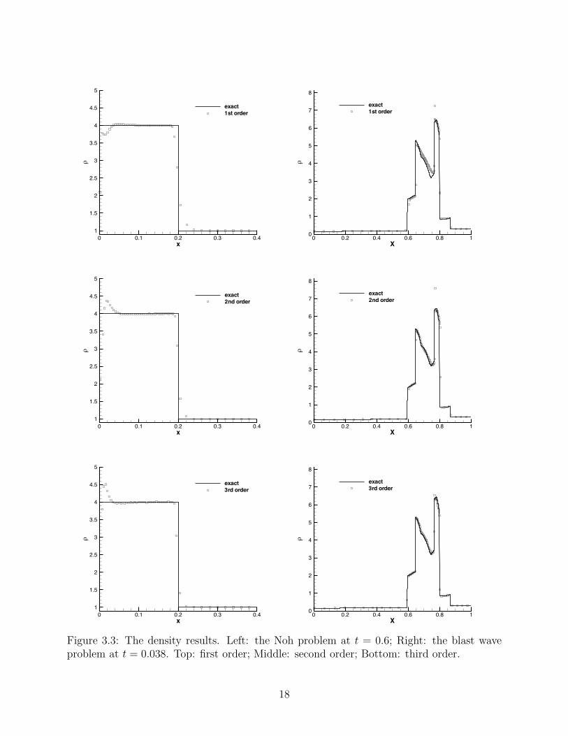
Example 3.2 (The Noh problem [22]). The computational domain is [0, 1]. The initial

state of the fluid is uniform with (ρ, u, e) = (1,−1, 0). The shock is generated in a perfect

ideal gas (γ = 5/3) by bringing the cold gas to rest at a rigid wall (x = 0). The analytic

post shock density is 4 and the shock speed is 1/3. The left pictures in Figure 3.3 show the

computational densities with 200 initially uniform cells against the exact density at t = 0.6.

We observe the typical errors near the left boundary for all orders of accuracy. The shock

resolution is clearly better for the higher order schemes.

Example 3.3 (Two interacting blast waves). The initial data are

ρ = 1, u = 1, p =

()

*

103, 0 < x < 0.110−2, 0.1 < x < 0.9102, 0.9 < x < 1.0.

The reflective boundary condition is applied at both x = 0 and x = 1. In the right pictures of

Figure 3.3, the computed densities with 400 initially uniform cells at the final time t = 0.038

are plotted against the reference “exact” solution, which is computed using a fifth order

Eulerian WENO scheme [15] with 16000 grid points. We can see the very satisfactory

resolution in the results of high order scheme with relatively coarse grids which demonstrates

the advantage of the Lagrangian scheme. Meanwhile, we observe some overshoots in these

17

x

!

0 0.1 0.2 0.3 0.41

1.5

2

2.5

3

3.5

4

4.5

5

exact1st order

X

!

0 0.2 0.4 0.6 0.8 10

1

2

3

4

5

6

7

8

exact1st order

x

!

0 0.1 0.2 0.3 0.41

1.5

2

2.5

3

3.5

4

4.5

5

exact2nd order

X

!

0 0.2 0.4 0.6 0.8 10

1

2

3

4

5

6

7

8

exact2nd order

x

!

0 0.1 0.2 0.3 0.41

1.5

2

2.5

3

3.5

4

4.5

5

exact3rd order

X

!

0 0.2 0.4 0.6 0.8 10

1

2

3

4

5

6

7

8

exact3rd order

Figure 3.3: The density results. Left: the Noh problem at t = 0.6; Right: the blast waveproblem at t = 0.038. Top: first order; Middle: second order; Bottom: third order.

18

figures and in some examples later. Apparently such overshoots are caused by the Lagrangian

framework rather than by the high order ENO reconstruction, since they are more serious

for the lower order schemes.

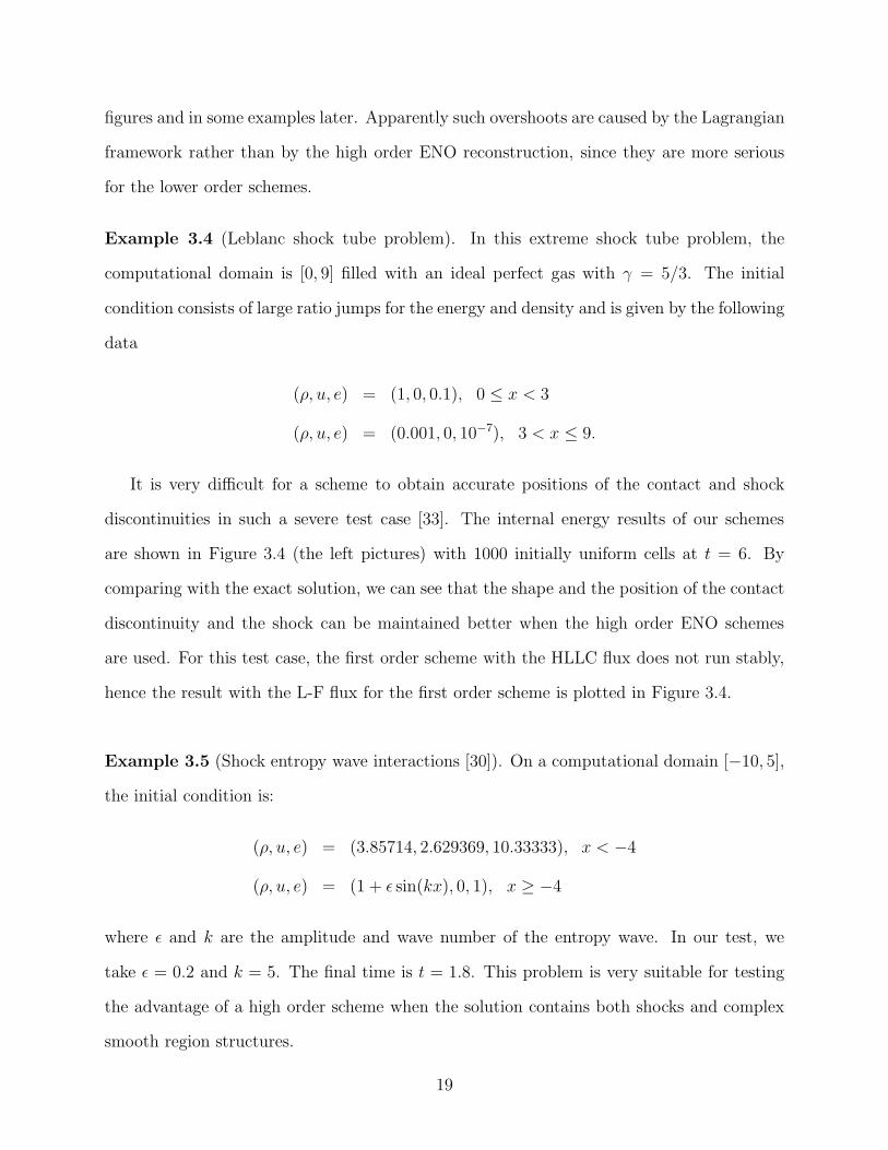
Example 3.4 (Leblanc shock tube problem). In this extreme shock tube problem, the

computational domain is [0, 9] filled with an ideal perfect gas with γ = 5/3. The initial

condition consists of large ratio jumps for the energy and density and is given by the following

data

(ρ, u, e) = (1, 0, 0.1), 0 ≤ x < 3

(ρ, u, e) = (0.001, 0, 10−7), 3 < x ≤ 9.

It is very difficult for a scheme to obtain accurate positions of the contact and shock

discontinuities in such a severe test case [33]. The internal energy results of our schemes

are shown in Figure 3.4 (the left pictures) with 1000 initially uniform cells at t = 6. By

comparing with the exact solution, we can see that the shape and the position of the contact

discontinuity and the shock can be maintained better when the high order ENO schemes

are used. For this test case, the first order scheme with the HLLC flux does not run stably,

hence the result with the L-F flux for the first order scheme is plotted in Figure 3.4.

Example 3.5 (Shock entropy wave interactions [30]). On a computational domain [−10, 5],

the initial condition is:

(ρ, u, e) = (3.85714, 2.629369, 10.33333), x < −4

(ρ, u, e) = (1 + ε sin(kx), 0, 1), x ≥ −4

where ε and k are the amplitude and wave number of the entropy wave. In our test, we

take ε = 0.2 and k = 5. The final time is t = 1.8. This problem is very suitable for testing

the advantage of a high order scheme when the solution contains both shocks and complex

smooth region structures.

19

X

e

0 50

0.05

0.1

0.15

0.2

exact1st order

X

!

-4 -2 0 2 4

1

1.5

2

2.5

3

3.5

4

4.5exact1st order

X

e

0 50

0.05

0.1

0.15

0.2

exact2nd order

X

!

-4 -2 0 2 4

1

1.5

2

2.5

3

3.5

4

4.5exact2nd order

X

e

0 50

0.05

0.1

0.15

0.2

exact3rd order

X

!

-4 -2 0 2 4

1

1.5

2

2.5

3

3.5

4

4.5exact3rd order

Figure 3.4: Left: the internal energy of the Leblanc problem; Right: the density of the shockentropy wave interactions problem. Top: first order; Middle: second order; Bottom: thirdorder.

20

In Figure 3.4 (the right pictures), the computed density with 400 cells is plotted against

the reference “exact” solution, which is obtained using the fifth order Eulerian WENO scheme

[15] with 2000 grid points. We observe that the fine structure in the density profile makes

the higher order schemes perform much better than the lower order methods.

4 High order ENO conservative Lagrangian scheme -two space dimensions

4.1 The scheme in the Cartesian coordinates

The 2D spatial domain Ω is discretized into M × N computational cells. Ii+1/2,j+1/2 is a

quadrilateral cell constructed by the four vertices (xi,j , yi,j), (xi+1,j , yi+1,j), (xi+1,j+1, yi+1,j+1),

(xi,j+1, yi,j+1). Si+1/2,j+1/2 is denoted to be the area of the cell Ii+1/2,j+1/2 with i = 1, . . . , M ,

j = 1, . . . , N . For a given cell Ii+1/2,j+1/2, the location of the cell center is denoted by

(xi+1/2,j+1/2, yi+1/2,j+1/2). The fluid velocity (ui,j, vi,j) is defined at the vertex of the mesh.

On the non-staggered mesh, all the variables except velocity are stored at the cell center of

Ii+1/2,j+1/2 in the form of cell averages. For example, the values of the cell averages for the

cell Ii+1/2,j+1/2 denoted by ρi+1/2,j+1/2, Mxi+1/2,j+1/2, M

yi+1/2,j+1/2 and Ei+1/2,j+1/2 are defined

as follows

ρi+1/2,j+1/2 =1

Si+1/2,j+1/2

!!

Ii+1/2,j+1/2

ρdxdy, Mxi+1/2,j+1/2 =

1

Si+1/2,j+1/2

!!

Ii+1/2,j+1/2

Mxdxdy,

Myi+1/2,j+1/2 =

1

Si+1/2,j+1/2

!!

Ii+1/2,j+1/2

Mydxdy, Ei+1/2,j+1/2 =1

Si+1/2,j+1/2

!!

Ii+1/2,j+1/2

Edxdy

where ρ, Mx, My and E are the density, x-momentum, y-momentum and total energy,

respectively.

21

4.1.1 Spatial discretization

The conservative semi-discrete scheme for the equations (2.1) and (2.4) has the following

form on the 2D non-staggered mesh

d

dt

"

&&#

ρi+1/2,j+1/2Si+1/2,j+1/2

Mxi+1/2,j+1/2Si+1/2,j+1/2

Myi+1/2,j+1/2Si+1/2,j+1/2

Ei+1/2,j+1/2Si+1/2,j+1/2

$

''% = −!

"Ii+1/2,j+1/2

Fdl

= −!

"Ii+1/2,j+1/2

"

&&&#

fD(U−n ,U+

n )fMx(U

−n ,U+

n )fMy(U

−n ,U+

n )fE(U−

n ,U+n )

$

'''% dl. (4.1)

Here n = (nx, ny) is the outward unit normal of the quadrilateral boundary ∂Ii+1/2,j+1/2.

U± = (ρ±, M±x , M±

y , E±) are the values of mass, x-momentum, y-momentum and total

energy at two sides of the boundary. U±n = (ρ±, M±

n , E±), where M±n are the left and

right component values of the momentum which is vertical to the cell boundary, i.e. M±n =

(M±x , M±

y ) · n. fD, fMx , fMy and fE are the numerical fluxes of mass, x-momentum, y-

momentum and total energy across the cell boundary respectively. Here in the Lagrangian

formulation, we have (+++)

+++*

fD(Un,Un) = 0,fMx(Un,Un) = pnx

fMy(Un,Un) = pny

fE(Un,Un) = pun

(4.2)

where un = u · n is the normal velocity at the cell boundary.

Suppose the cell boundary ∂Ii+1/2,j+1/2 consists of M edges. The line integral in Eq. (4.1)

is discretized by a q-point Gaussian integration formula,

!

"Ii+1/2,j+1/2

Fdl ≈M-

m=1

q-

k=1

ωkF(Un(Gk, t))∆lm (4.3)

where ∆lm is the length of the boundary edge m and Gk are the Gaussian quadrature points

at the edge. Here F(Un(Gk, t)) is a numerical flux. For example the L-F flux is given by

F(Un(Gk, t)) =1

2[(F(U−

n (Gk, t)) + F(U+n (Gk, t))) − α(U+(Gk, t) − U−(Gk, t))] (4.4)

22

where α has the same meaning as that in the one dimensional case.

We use the high order ENO reconstruction with Roe-type characteristic decomposition

[31] to obtain U± and U±n at the boundary and also use sufficiently high order quadrature to

construct schemes up to the expected high-order spatial accuracy, for example the four-point

Gauss-Lobatto integral formula is used, which has G1 = P1, G2 = 12(P1 +P2)−

√5

10 (P2 −P1),

G3 = 12(P1 + P2) +

√5

10 (P2 − P1), G4 = P2 and ω1 = ω4 = 112 , ω2 = ω3 = 5

12 for the line

with endpoints P1 and P2. We have discussed in detail the high order ENO reconstruction

needed in our framework in [7], in the context of remapping. Therefore we do not repeat

the details here and refer the readers to [7]. We do mention here, however, that we have

found in numerical tests that the following WENO procedure is more robust than the ENO

procedure for the third order case, hence this WENO procedure is used in the third order

numerical tests. In this procedure, the coefficients of the reconstruction polynomial are

chosen as the weighted averages of those determined by the final three possible stencils

introduced in [7]. To be more specific, we use density as an example. To determine the

coefficients amn, m+n ≤ 2 of the quadratic polynomial reconstruction function inside the

cell Ii+1/2,j+1/2,

ρi+1/2,j+1/2(x, y) =-

m+n≤2

amn(x − xi+1/2,j+1/2)m(y − yi+1/2,j+1/2)

n,

suppose the coefficients of the reconstruction polynomials of the three candidate stencils are

aimn, i = 1, 2, 3, then we choose amn =

.3i=1 wiai

mn where wi is the weight chosen as wi =

(1/.

m+n=2 |aimn|2)/c with c =

.3i=1(1/

.m+n=2 |ai

mn|2). This crude WENO reconstruction,

which does not increase the accuracy of each candidate stencil but is very easy to compute,

performs quite nicely in our numerical experiments.

The three numerical fluxes introduced in the one dimensional case are also applied here.

The form of these fluxes in two dimensions is similar to that in one dimension except that

the left and right values at the cell’s boundary are chosen as U±n in two dimensions rather

than U± in one dimension.

23

4.1.2 The determination of the vertex velocity

Considering a vertex (i, j) shared by four edges which are given a serial number k = 1, 2, 3, 4,

we define the direction of each edge to be the direction of the incremental index i or j, for ex-

ample the direction of the edge with two endpoints (i−1, j) and (i, j) is from (i−1, j) to (i, j).

Along each edge k we can obtain the left value of velocity (uk−, vk−) = (Mk−x /ρk−, Mk−

y /ρk−)

and the right velocity (uk+, vk+) = (Mk+x /ρk+, Mk+

y /ρk+) at this vertex in the procedure of

the flux computation since the vertex (i, j) is one of the Gaussian quadrature points for our

choice. We then split the left and right velocities into vertical and tangential components

along the edge k. Denote (nkx, n

ky) to be the clockwise unit normal of the edge k and de-

note wk−t and wk+

t to be their tangential components and wk−n and wk+

n to be their vertical

components. Then the tangential velocity of the vertex (i, j) along the edge k is defined as

wkt =

1

2(wk−

t + wk+t ), k = 1, 2, 3, 4. (4.5)

As to the vertical velocity, for the Godunov flux, we get it by the Riemann solver here

and for the L-F flux and the HLLC flux, we get it by the Roe average of the vertical velocities

from its two sides as in the one dimensional case, that is

wkn =

√ρ−wk−

n +√ρ+wk+

n√ρ− +

√ρ+

, k = 1, 2, 3, 4, (4.6)

where ρ± are the densities from the left and right cells of the edge k respectively.

Thus by the formulas (4.5) and (4.6), we can get four x-velocities and y-velocities at the

vertex (i, j) which have the following form,

wkx = wk

nnkx − wk

t nky, wk

y = wknnk

y + wkt n

kx, k = 1, 2, 3, 4. (4.7)

Finally the velocity at the vertex (i, j) is obtained as follows,

ui,j =1

4(w1

x + w2x + w3

x + w4x), vi,j =

1

4(w1

y + w2y + w3

y + w4y). (4.8)

24

4.1.3 Time discretization

The time discretization is also similar to that in one dimension. We only list the first order

Lagrangian scheme as a representative here to save space"

&&&&#

ρn+1i+1/2,j+1/2S

n+1i+1/2,j+1/2 − ρn

i+1/2,j+1/2Sni+1/2,j+1/2

Mx,n+1i+1/2,j+1/2S

n+1i+1/2,j+1/2 − M

x,ni+1/2,j+1/2S

ni+1/2,j+1/2

My,n+1i+1/2,j+1/2S

n+1i+1/2,j+1/2 − M

y,ni+1/2,j+1/2S

ni+1/2,j+1/2

En+1i+1/2,j+1/2S

n+1i+1/2,j+1/2 − E

ni+1/2,j+1/2S

ni+1/2,j+1/2

$

''''%= −∆tn

M-

m=1

q-

k=1

ωkF(Un(Gk, t))∆lm

(4.9)

where Sni+1/2,j+1/2 and Sn+1

i+1/2,j+1/2 are the areas of Cell Ii+1/2,j+1/2 at the n-th and (n + 1)-th

time steps respectively. Sn+1i+1/2,j+1/2 is determined by the following simple formulas,

xn+1i,j = un

i,j∆tn + xni,j, yn+1

i,j = vni,j∆tn + yn

i,j,

Sn+1i,j =

1

2[(xn+1

i+1,j+1 − xn+1i,j )(yn+1

i,j+1 − yn+1i+1,j) + (xn+1

i,j+1 − xn+1i+1,j)(y

n+1i+1,j+1 − yn+1

i,j )],

i = 1, . . . , M, j = 1, . . . , N. (4.10)

The time step ∆tn is chosen as follows

∆tn = λ mini=1,...,M,j=1,...,N

(∆lni+1/2,j+1/2/cni+1/2,j+1/2) (4.11)

where ∆lni+1/2,j+1/2 is the shortest edge length of the cell Ii+1/2,j+1/2, and cni+1/2,j+1/2 is the

sound speed within this cell. The Courant number λ in the following tests is set to be 0.5

unless otherwise stated.

4.2 The scheme in the cylindrical coordinates

We seek to study the flow governed by the axisymmetric compressible Euler equations which

have the following integral form in the Lagrangian formulation,

(+++++)

+++++*

ddt

//Ω(t) ρrdxdr = 0

ddt

//Ω(t) Mxrdxdr = −

/Γ(t) pnxrdl

ddt

//Ω(t) Mrrdxdr = −

/Γ(t) pnrrdl +

//Ω(t)(p + ρu2

#)dxdrddt

//Ω(t) M#rdxdr = −

//Ω(t) ρu#urdxdr

ddt

//Ω(t) Erdxdr = −

/Γ(t) punrdl

(4.12)

25

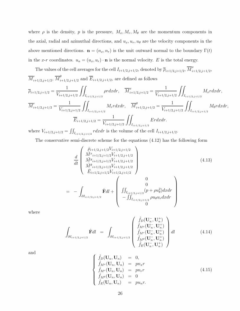
where ρ is the density, p is the pressure, Mx, Mr, M# are the momentum components in

the axial, radial and azimuthal directions, and ux, ur, u# are the velocity components in the

above mentioned directions. n = (nx, nr) is the unit outward normal to the boundary Γ(t)

in the x-r coordinates. un = (ux, ur) · n is the normal velocity. E is the total energy.

The values of the cell averages for the cell Ii+1/2,j+1/2, denoted by ρi+1/2,j+1/2, Mxi+1/2,j+1/2,

Mri+1/2,j+1/2, M

#i+1/2,j+1/2 and Ei+1/2,j+1/2, are defined as follows

ρi+1/2,j+1/2 =1

Vi+1/2,j+1/2

!!

Ii+1/2,j+1/2

ρrdxdr, Mxi+1/2,j+1/2 =

1

Vi+1/2,j+1/2

!!

Ii+1/2,j+1/2

Mxrdxdr,

Mri+1/2,j+1/2 =

1

Vi+1/2,j+1/2

!!

Ii+1/2,j+1/2

Mrrdxdr, M#i+1/2,j+1/2 =

1

Vi+1/2,j+1/2

!!

Ii+1/2,j+1/2

M#rdxdr,

Ei+1/2,j+1/2 =1

Vi+1/2,j+1/2

!!

Ii+1/2,j+1/2

Erdxdr.

where Vi+1/2,j+1/2 =//

Ii+1/2,j+1/2rdxdr is the volume of the cell Ii+1/2,j+1/2.

The conservative semi-discrete scheme for the equations (4.12) has the following form

d

dt

"

&&&&#

ρi+1/2,j+1/2Vi+1/2,j+1/2

Mxi+1/2,j+1/2Vi+1/2,j+1/2

Myi+1/2,j+1/2Vi+1/2,j+1/2

M#i+1/2,j+1/2Vi+1/2,j+1/2

Ei+1/2,j+1/2Vi+1/2,j+1/2

$

''''%(4.13)

= −!

"Ii+1/2,j+1/2

Fdl +

"

&&&&&#

00//

Ii+1/2,j+1/2(p + ρu2

#)dxdr

−//

Ii+1/2,j+1/2ρu#urdxdr

0

$

'''''%

where

!

"Ii+1/2,j+1/2

Fdl =

!

"Ii+1/2,j+1/2

"

&&&&&#

fD(U−n ,U+

n )fMx(U−

n ,U+n )

fMr(U−n ,U+

n )fMθ(U−

n ,U+n )

fE(U−n ,U+

n )

$

'''''%dl (4.14)

and (+++++)

+++++*

fD(Un,Un) = 0,fMx(Un,Un) = pnxrfMr(Un,Un) = pnrrfMθ(Un,Un) = 0fE(Un,Un) = punr.

(4.15)

26

The calculation of the first term on the right hand side of Eq. (4.13) is similar to that in

the Cartesian coordinates introduced in the above subsection. The calculation of the second

term is performed by a suitable Gaussian integral in the corresponding cell to guarantee its

high-order accurate approximation.

We use the same method as that used in the Cartesian coordinates to decide the velocity

components (ux, ur) at the vertex in the x and r directions (since the grid moves just in the

x-r coordinates, we only need to know ux, ur).

We also use the Runge-Kutta method to discretize the time derivatives in (4.13). The

method to calculate the time step is the same as that in the Cartesian coordinates.

5 Numerical results in two space dimensions

It is much more difficult to simulate a 2D problem than to simulate a 1D one in the La-

grangian framework, mainly because of the mesh distortion in multi-dimensions. In this

section, although we have run most examples using the first, second and third order schemes

with the Godunov flux, the HLLC flux and the L-F flux respectively, we did unfortunately

observe that for some very tough problems simulations with some of the fluxes such as the

Godunov flux cannot run in a stable fashion. Since the L-F flux shows its best robustness in

our simulation of 2D problems among these fluxes, we will only show the results performed

by the L-F flux as representatives, although the results may not be the best for individual

test cases among those using these three fluxes.

5.1 Numerical results in the Cartesian coordinates

5.1.1 Accuracy test

In the Cartesian coordinates, we choose the two-dimensional vortex evolution problem [28]

as our accuracy test function. The vortex problem is described as follows: The mean flow

is ρ = 1, p = 1 and (u, v) = (1, 1) (diagonal flow). We add to this mean flow an isentropic

vortex perturbations in (u, v) and the temperature T = p/ρ, no perturbation in the entropy

27

S = p/ρ$.

(δu, δv) =ε

2πe0.5(1−r2)(−y, x), δT = −(γ − 1)ε2

8γπ2e(1−r2), δS = 0

where (−y, x) = (x − 5, y − 5), r2 = x2 + y2, and the vortex strength is ε = 5.

The computational domain is taken as [0, 10]× [0, 10], and periodic boundary conditions

are used.

The convergence results for the first, second and third order ENO Lagrangian schemes at

t = 1 are listed in Tables 5.1-5.3 respectively. In Tables 5.1 and 5.2, we can see the desired

first and second order accuracy. However in Table 5.3 we cannot observe the expected third

order accuracy. Further exploration indicates that this accuracy degeneracy cannot be cured

by the modified ENO scheme via the introduction of a biasing factor in the stencil-choosing

process. It represents a fundamental problem in our way of formulating the Lagrangian

schemes. In a Lagrangian simulation, each cell represents a material particle, thus its shape

may change with the movement of fluid, that means the cell with a quadrilateral shape

initially may not keep its shape as a quadrilateral at a later time. It usually becomes a curved

quadrilateral, while during our Lagrangian simulation the mesh is always supposed to be

quadrilateral which is determined by the movement of its four vertices. This approximation

of the mesh will bring second order error into the scheme. Thus for a Lagrangian scheme

in multi-dimensions, it can be at most second order accurate if curved meshes are not used.

We will not explore curved meshes in this paper, hence our “third order” scheme is indeed

only second order accurate. However, in the following examples, we indeed often find better

resolution in the fluid field by the third order scheme compared with that obtained by the

lower order schemes, despite its formal second order accuracy.

5.1.2 Non-oscillatory tests

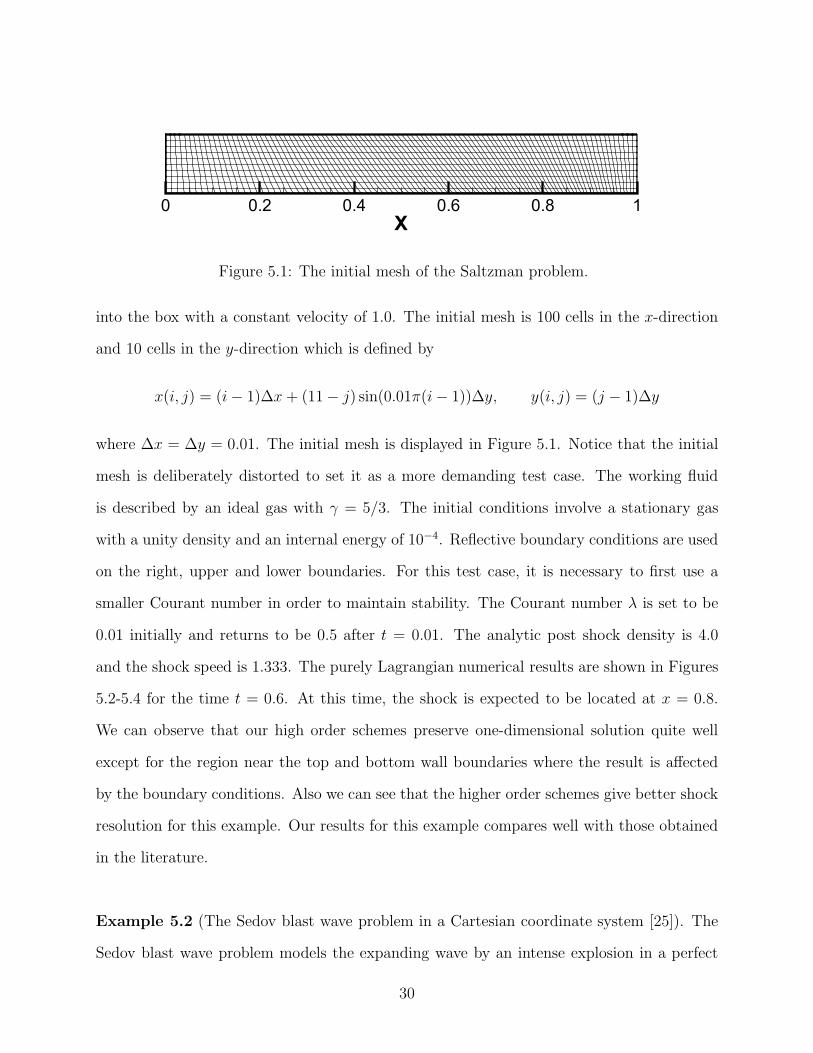
Example 5.1 (The Saltzman problem [10]). This is a well known difficult test case to

validate the robustness of a Lagrangian scheme when the mesh is not aligned with the fluid

flow. The problem consists of a rectangular box whose left end is a piston. The piston moves

28

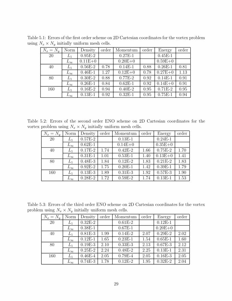
Table 5.1: Errors of the first order scheme on 2D Cartesian coordinates for the vortex problemusing Nx × Ny initially uniform mesh cells.

Nx = Ny Norm Density order Momentum order Energy order20 L1 0.95E-2 0.27E-1 0.45E-1

L∞ 0.11E+0 0.20E+0 0.59E+040 L1 0.56E-2 0.78 0.14E-1 0.88 0.26E-1 0.81

L∞ 0.46E-1 1.27 0.12E+0 0.78 0.27E+0 1.1380 L1 0.30E-2 0.88 0.77E-2 0.92 0.14E-1 0.91

L∞ 0.26E-1 0.84 0.62E-1 0.92 0.14E+0 0.91160 L1 0.16E-2 0.94 0.40E-2 0.95 0.71E-2 0.95

L∞ 0.13E-1 0.92 0.32E-1 0.95 0.75E-1 0.94

Table 5.2: Errors of the second order ENO scheme on 2D Cartesian coordinates for thevortex problem using Nx × Ny initially uniform mesh cells.

Nx = Ny Norm Density order Momentum order Energy order20 L1 0.57E-2 0.13E-1 0.24E-1

L∞ 0.62E-1 0.14E+0 0.35E+040 L1 0.17E-2 1.74 0.42E-2 1.66 0.75E-2 1.70

L∞ 0.31E-1 1.01 0.53E-1 1.40 0.13E+0 1.4180 L1 0.48E-3 1.84 0.12E-2 1.83 0.21E-2 1.83

L∞ 0.92E-2 1.75 0.20E-1 1.42 0.39E-1 1.79160 L1 0.13E-3 1.89 0.31E-3 1.92 0.57E-3 1.90

L∞ 0.28E-2 1.72 0.59E-2 1.74 0.13E-1 1.53

Table 5.3: Errors of the third order ENO scheme on 2D Cartesian coordinates for the vortexproblem using Nx × Ny initially uniform mesh cells.

Nx = Ny Norm Density order Momentum order Energy order20 L1 0.32E-2 0.61E-2 0.12E-1

L∞ 0.38E-1 0.67E-1 0.20E+040 L1 0.81E-3 1.99 0.14E-2 2.07 0.29E-2 2.02

L∞ 0.12E-1 1.65 0.23E-1 1.54 0.65E-1 1.6080 L1 0.19E-3 2.10 0.33E-3 2.13 0.67E-3 2.12

L∞ 0.25E-2 2.24 0.48E-2 2.25 0.13E-1 2.31160 L1 0.46E-4 2.05 0.79E-4 2.05 0.16E-3 2.05

L∞ 0.74E-3 1.78 0.12E-2 1.95 0.32E-2 2.04

29

X0 0.2 0.4 0.6 0.8 1

Figure 5.1: The initial mesh of the Saltzman problem.

into the box with a constant velocity of 1.0. The initial mesh is 100 cells in the x-direction

and 10 cells in the y-direction which is defined by

x(i, j) = (i − 1)∆x + (11 − j) sin(0.01π(i − 1))∆y, y(i, j) = (j − 1)∆y

where ∆x = ∆y = 0.01. The initial mesh is displayed in Figure 5.1. Notice that the initial

mesh is deliberately distorted to set it as a more demanding test case. The working fluid

is described by an ideal gas with γ = 5/3. The initial conditions involve a stationary gas

with a unity density and an internal energy of 10−4. Reflective boundary conditions are used

on the right, upper and lower boundaries. For this test case, it is necessary to first use a

smaller Courant number in order to maintain stability. The Courant number λ is set to be

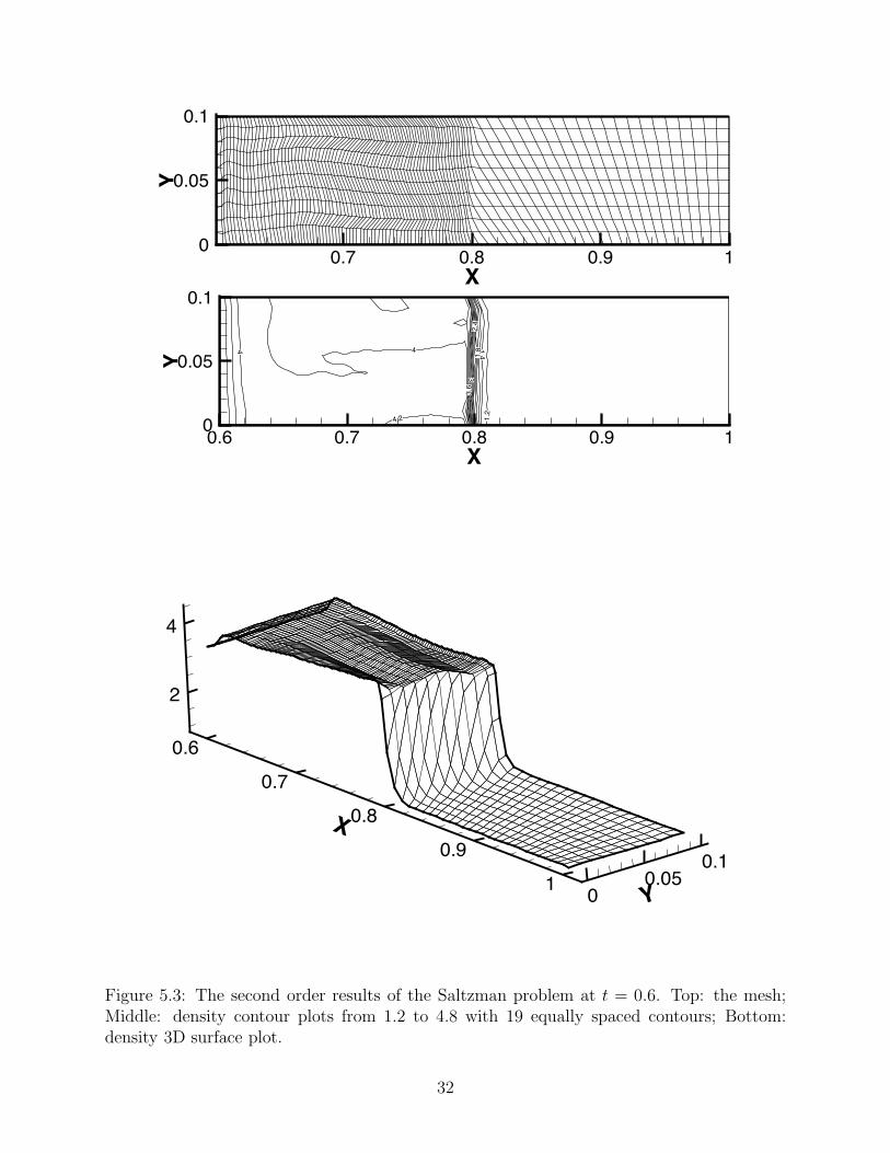
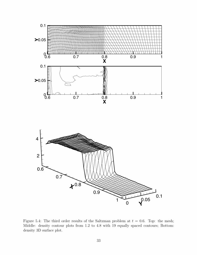
0.01 initially and returns to be 0.5 after t = 0.01. The analytic post shock density is 4.0

and the shock speed is 1.333. The purely Lagrangian numerical results are shown in Figures

5.2-5.4 for the time t = 0.6. At this time, the shock is expected to be located at x = 0.8.

We can observe that our high order schemes preserve one-dimensional solution quite well

except for the region near the top and bottom wall boundaries where the result is affected

by the boundary conditions. Also we can see that the higher order schemes give better shock

resolution for this example. Our results for this example compares well with those obtained

in the literature.

Example 5.2 (The Sedov blast wave problem in a Cartesian coordinate system [25]). The

Sedov blast wave problem models the expanding wave by an intense explosion in a perfect

30

X

Y

0.6 0.7 0.8 0.9 10

0.05

0.1

1.41.8

2.2

2.4

3.2

3.4

3.6

3.8

4

4.24.44.64 8

X

Y

0.6 0.7 0.8 0.9 10

0.05

0.1

X

0.60.7

0.80.9

1Y00.05

0.1

2

4

Figure 5.2: The first order results of the Saltzman problem at t = 0.6. Top: the mesh;Middle: density contour plots from 1.2 to 4.8 with 19 equally spaced contours; Bottom:density 3D surface plot.

31

X

Y

0.7 0.8 0.9 10

0.05

0.1

1.2

1.41.8

2.4

3

3.6

4 4

4.2

X

Y

0.6 0.7 0.8 0.9 10

0.05

0.1

X

0.60.7

0.80.9

1 Y00.05

0.1

2

4

Figure 5.3: The second order results of the Saltzman problem at t = 0.6. Top: the mesh;Middle: density contour plots from 1.2 to 4.8 with 19 equally spaced contours; Bottom:density 3D surface plot.

32

X

Y

0.6 0.7 0.8 0.9 10

0.05

0.1

1.6

2.4

2.6

3

3.6

3.8

4

4

4

X

Y

0.6 0.7 0.8 0.9 10

0.05

0.1

X

0.60.7

0.80.9

1Y00.05

0.1

2

4

Figure 5.4: The third order results of the Saltzman problem at t = 0.6. Top: the mesh;Middle: density contour plots from 1.2 to 4.8 with 19 equally spaced contours; Bottom:density 3D surface plot.

33

gas. The simulation is first performed on a Cartesian grid whose initial uniform grid consists

of 30 × 30 rectangular cells with a total edge length of 1.1 in both directions. The initial

density is unity and the initial velocity is zero. The specific internal energy is zero except in

the first zone where it has a value of 182.09. The analytical solution gives a shock at radius

unity at time unity with a peak density of 6. Figure 5.5 shows the results by the purely

Lagrangian calculations at the time t = 1. We can clearly see that the high order ENO

scheme obtains higher peak density than the lower order one.

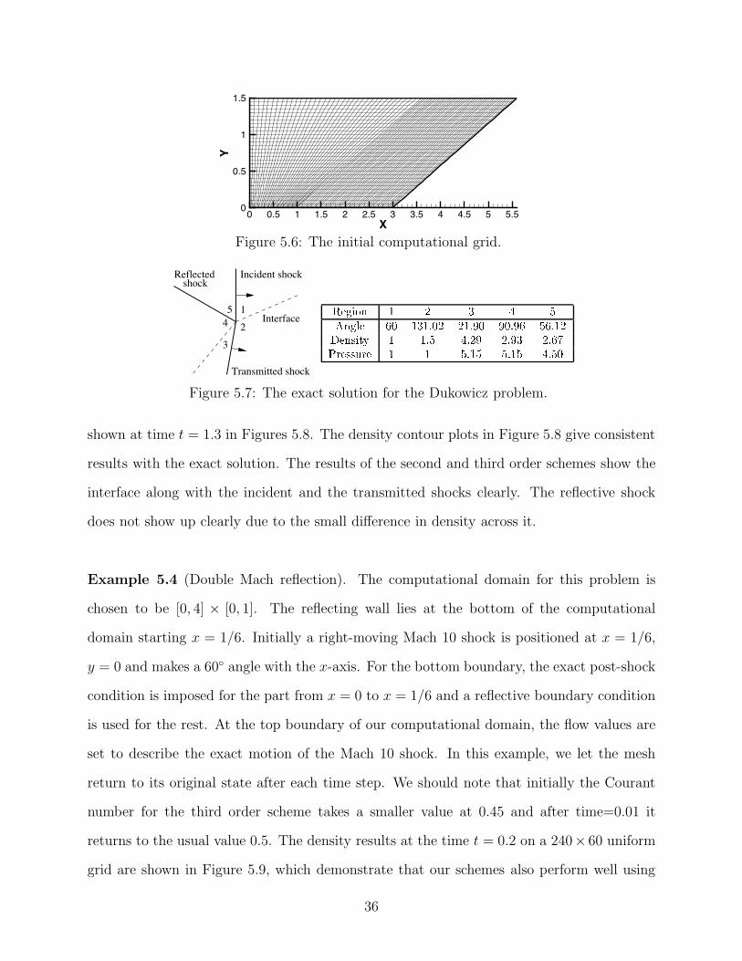
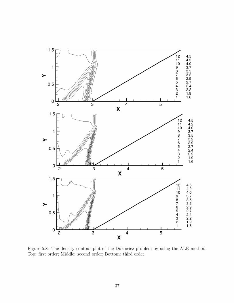
Example 5.3 (The Dukowicz problem). In this and the next examples, we will test the

performance of our scheme in the ALE calculations. At each time step, we first use our

Lagrangian scheme to update the solution and mesh, then we rezone the Lagrangian mesh

to a more optimal position and finally remap the Lagrangian solutions to the new grid. The

conservative remapping method is also based on the ENO methodology and is described in

detail in [7]. The Dukowicz problem is a two dimensional shock refraction problem on an

uneven mesh designed by Dukowicz and Meltz [10].

The computational domain consists of two adjacent regions with different densities but

equal pressures. The left region is a 36 × 30 mesh with a vertical left boundary and a right

boundary aligned at 30 to the horizontal direction. The right region is a 40 × 30 mesh

uniformly slanted at 30 to the horizontal direction. See Figure 5.6. The initial conditions

of the two regions are ρL = 1, uL = 0, pL = 1 and ρR = 1, uR = 0, pR = 1.5 respectively. The

upper and lower boundaries are reflective and the left boundary is a piston, which moves

from the left with velocity 1.48. The problem is run to a time of 1.3, just before the shock

would leave the right region. The exact solution to the problem is shown in Figure 5.7 which

is only valid away from the boundary as it is obtained under the assumption of an infinite

medium. In this test, when the area of the minimum cell is less than 4×10−4, we rezone the

meshes by keeping the vertices at the left and right boundaries unchanged and redistributing

the points in the x direction evenly. The numerical results using the ALE calculations are

34

X

Y

0 0.2 0.4 0.6 0.8 10

0.1

0.2

0.3

0.4

0.5

0.6

0.7

0.8

0.9

1

1.1

1

1

2

2

3

3

3

3

3

4

4

4

4

4

5

5

5

5

6

6

6

6

6

6

7

7

7

7

7

8

8

8

8

8

9

9

9

9

9

10

10

10

10

10

11

11 11

11

12

12

12

12

12

X

Y

0 0.2 0.4 0.6 0.8 10

0.1

0.2

0.3

0.4

0.5

0.6

0.7

0.8

0.9

1

1.1

14 5.613 5.212 4.811 4.410 49 3.68 3.27 2.86 2.45 24 1.63 1.22 0.81 0.4

r

!

0 0.5 1 1.5

1

2

3

4

5

X

Y

0 0.2 0.4 0.6 0.8 10

0.1

0.2

0.3

0.4

0.5

0.6

0.7

0.8

0.9

1

1.1

1

1

2

2

3

3

3

3

4

4

4

4

5

5

5

5

5

6

6

6

6

6

7

7

7

7

7

8

8

8

8

8

9

9

9

9

10

10

10

10

10

11

11

11

11

11

12

12

12

12

12

13

X

Y

0 0.2 0.4 0.6 0.8 10

0.1

0.2

0.3

0.4

0.5

0.6

0.7

0.8

0.9

1

1.114 5.613 5.212 4.811 4.410 49 3.68 3.27 2.86 2.45 24 1.63 1.22 0.81 0.4

r

!

0 0.5 1 1.5

1

2

3

4

5

X

Y

0 0.2 0.4 0.6 0.8 10

0.1

0.2

0.3

0.4

0.5

0.6

0.7

0.8

0.9

1

1.1

1

1

2

2

3

3

3

3

3

4

4

4

4

5

5

5

5

6

6

6

6

6

7

7

7

7

7

8

8

8

8

8

8

9

9

9

9

9

10

10

10

10

10

10

11

11

11

11

11

11

12

12

12

12

13

X

Y

0 0.2 0.4 0.6 0.8 10

0.1

0.2

0.3

0.4

0.5

0.6

0.7

0.8

0.9

1

1.114 5.613 5.212 4.811 4.410 49 3.68 3.27 2.86 2.45 24 1.63 1.22 0.81 0.4

r

!

0 0.5 1 1.5

1

2

3

4

5

Figure 5.5: The Sedov problem at t = 1. Top: the first order results; Middle: the secondorder results; Bottom: the third order results. Left: the mesh; Middle: density contours;Right: density as a function of the radius.

35

XY

0 0.5 1 1.5 2 2.5 3 3.5 4 4.5 5 5.50

0.5

1

1.5

Figure 5.6: The initial computational grid.

Incident shock

Interface

Transmitted shock

Reflectedshock

12

3

45

Figure 5.7: The exact solution for the Dukowicz problem.

shown at time t = 1.3 in Figures 5.8. The density contour plots in Figure 5.8 give consistent

results with the exact solution. The results of the second and third order schemes show the

interface along with the incident and the transmitted shocks clearly. The reflective shock

does not show up clearly due to the small difference in density across it.

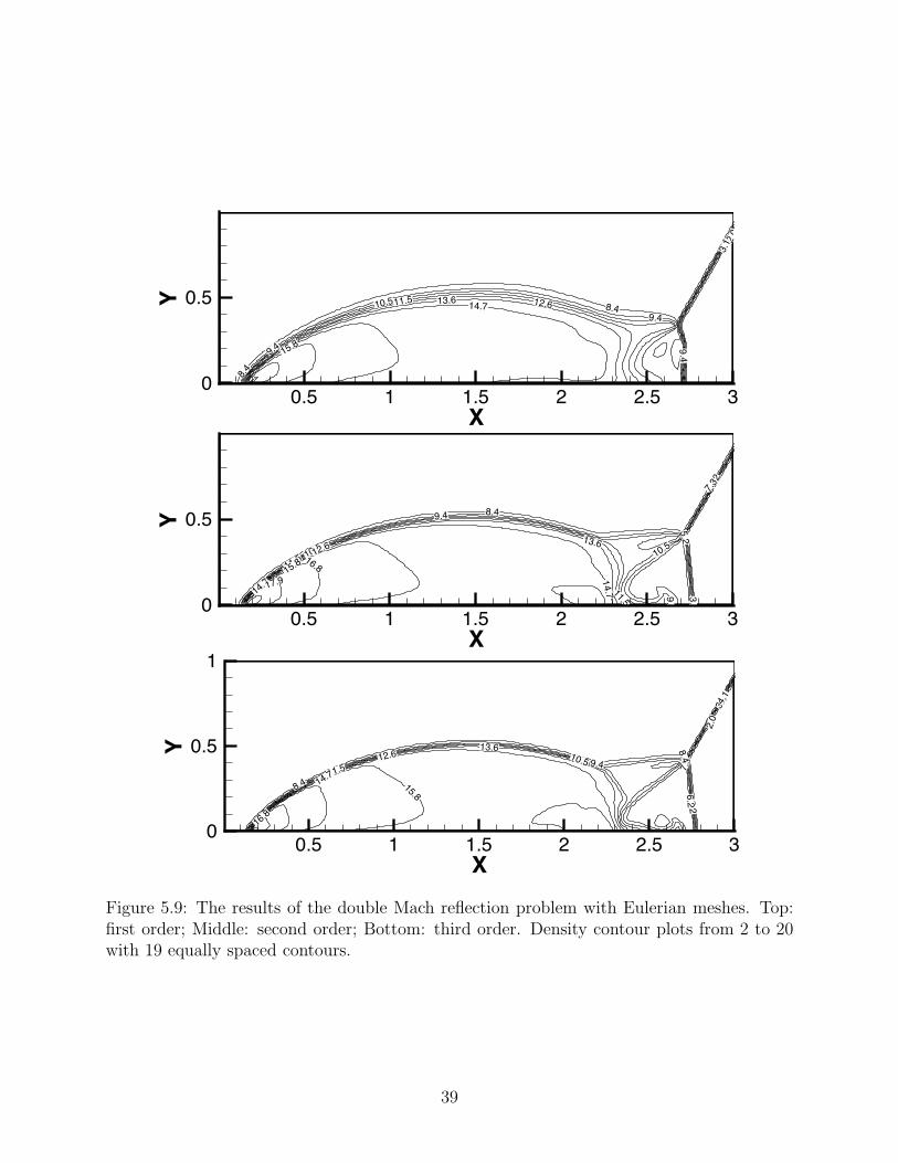
Example 5.4 (Double Mach reflection). The computational domain for this problem is

chosen to be [0, 4] × [0, 1]. The reflecting wall lies at the bottom of the computational

domain starting x = 1/6. Initially a right-moving Mach 10 shock is positioned at x = 1/6,

y = 0 and makes a 60 angle with the x-axis. For the bottom boundary, the exact post-shock

condition is imposed for the part from x = 0 to x = 1/6 and a reflective boundary condition

is used for the rest. At the top boundary of our computational domain, the flow values are

set to describe the exact motion of the Mach 10 shock. In this example, we let the mesh

return to its original state after each time step. We should note that initially the Courant

number for the third order scheme takes a smaller value at 0.45 and after time=0.01 it

returns to the usual value 0.5. The density results at the time t = 0.2 on a 240× 60 uniform

grid are shown in Figure 5.9, which demonstrate that our schemes also perform well using

36

12

3

34

5

5

6

6

7

7

8

8

9

9

10

X

Y

2 3 4 50

0.5

1

1.512 4.511 4.210 4.09 3.78 3.57 3.26 2.95 2.74 2.43 2.22 1.91 1.6

1

2

3

4

4

5

56

6

6

7

8

8

9

9

10

10

11

X

Y

2 3 4 50

0.5

1

1.512 4.511 4.210 4.09 3.78 3.57 3.26 2.95 2.74 2.43 2.22 1.91 1.6

1

2

23

4

5

5

6

6

6

7

78

9

9

10

10

11

X

Y

2 3 4 50

0.5

1

1.512 4.511 4.210 4.09 3.78 3.57 3.26 2.95 2.74 2.43 2.22 1.91 1.6

Figure 5.8: The density contour plot of the Dukowicz problem by using the ALE method.Top: first order; Middle: second order; Bottom: third order.

37

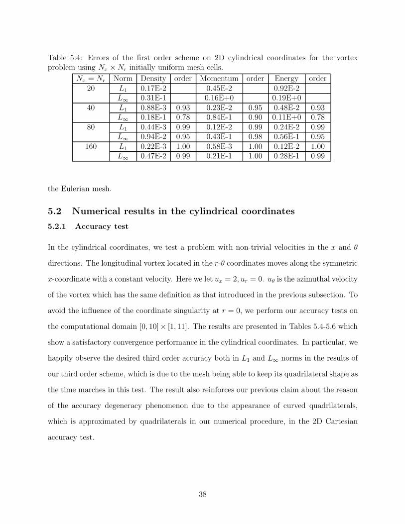
Table 5.4: Errors of the first order scheme on 2D cylindrical coordinates for the vortexproblem using Nx × Nr initially uniform mesh cells.

Nx = Nr Norm Density order Momentum order Energy order20 L1 0.17E-2 0.45E-2 0.92E-2

L∞ 0.31E-1 0.16E+0 0.19E+040 L1 0.88E-3 0.93 0.23E-2 0.95 0.48E-2 0.93

L∞ 0.18E-1 0.78 0.84E-1 0.90 0.11E+0 0.7880 L1 0.44E-3 0.99 0.12E-2 0.99 0.24E-2 0.99

L∞ 0.94E-2 0.95 0.43E-1 0.98 0.56E-1 0.95160 L1 0.22E-3 1.00 0.58E-3 1.00 0.12E-2 1.00

L∞ 0.47E-2 0.99 0.21E-1 1.00 0.28E-1 0.99

the Eulerian mesh.

5.2 Numerical results in the cylindrical coordinates

5.2.1 Accuracy test

In the cylindrical coordinates, we test a problem with non-trivial velocities in the x and θ

directions. The longitudinal vortex located in the r-θ coordinates moves along the symmetric

x-coordinate with a constant velocity. Here we let ux = 2, ur = 0. u# is the azimuthal velocity

of the vortex which has the same definition as that introduced in the previous subsection. To

avoid the influence of the coordinate singularity at r = 0, we perform our accuracy tests on

the computational domain [0, 10]× [1, 11]. The results are presented in Tables 5.4-5.6 which

show a satisfactory convergence performance in the cylindrical coordinates. In particular, we

happily observe the desired third order accuracy both in L1 and L∞ norms in the results of

our third order scheme, which is due to the mesh being able to keep its quadrilateral shape as

the time marches in this test. The result also reinforces our previous claim about the reason

of the accuracy degeneracy phenomenon due to the appearance of curved quadrilaterals,

which is approximated by quadrilaterals in our numerical procedure, in the 2D Cartesian

accuracy test.

38

2.0

3.1

8.4

8.4

9.4

9.4

9.4

10.511.5 12.613.6 14.7

15.8

X

Y

0.5 1 1.5 2 2.5 30

0.5

3.5.2

6.2

7.3

8.49.4

9.4

10.5 10.5

11.5

11.5

12.613.6

14.7 14.7

15.8 16.8

17.9

X

Y

0.5 1 1.5 2 2.5 30

0.5

2.03.14.1

5.26.2

7.3

8.4

8.49.410.5

11.512.6

13.6

14.7

15.8

16.8

X

Y

0.5 1 1.5 2 2.5 30

0.5

1

Figure 5.9: The results of the double Mach reflection problem with Eulerian meshes. Top:first order; Middle: second order; Bottom: third order. Density contour plots from 2 to 20with 19 equally spaced contours.

39

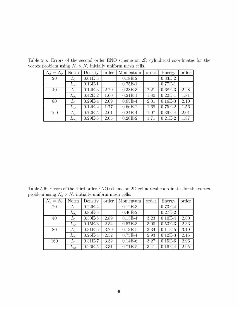
Table 5.5: Errors of the second order ENO scheme on 2D cylindrical coordinates for thevortex problem using Nx × Nr initially uniform mesh cells.

Nx = Nr Norm Density order Momentum order Energy order20 L1 0.61E-3 0.18E-2 0.33E-2

L∞ 0.13E-1 0.75E-1 0.77E-140 L1 0.12E-3 2.29 0.38E-3 2.21 0.68E-3 2.28

L∞ 0.42E-2 1.60 0.21E-1 1.80 0.22E-1 1.8180 L1 0.29E-4 2.09 0.95E-4 2.01 0.16E-3 2.10

L∞ 0.12E-2 1.77 0.66E-2 1.69 0.75E-2 1.56160 L1 0.72E-5 2.01 0.24E-4 1.97 0.39E-4 2.01

L∞ 0.29E-3 2.05 0.20E-2 1.71 0.21E-2 1.87

Table 5.6: Errors of the third order ENO scheme on 2D cylindrical coordinates for the vortexproblem using Nx × Nr initially uniform mesh cells.

Nx = Nr Norm Density order Momentum order Energy order20 L1 0.22E-4 0.12E-3 0.73E-4

L∞ 0.86E-3 0.46E-2 0.27E-240 L1 0.30E-5 2.89 0.13E-4 3.23 0.10E-4 2.80

L∞ 0.15E-3 2.54 0.57E-3 3.00 0.53E-3 2.3380 L1 0.31E-6 3.29 0.13E-5 3.34 0.11E-5 3.19

L∞ 0.26E-4 2.52 0.75E-4 2.93 0.12E-3 2.15160 L1 0.31E-7 3.32 0.14E-6 3.27 0.15E-6 2.96

L∞ 0.26E-5 3.31 0.71E-5 3.41 0.16E-4 2.95

40

r

!

0 0.05 0.1 0.15 0.2 0.25 0.3 0.35

2

4

6

8

10

12

14

16 exact1st order

r

!

0 0.05 0.1 0.15 0.2 0.25 0.3 0.35

2

4

6

8

10

12

14

16 exact2nd order

r

!

0 0.05 0.1 0.15 0.2 0.25 0.3 0.35

2

4

6

8

10

12

14

16 exact3rd order

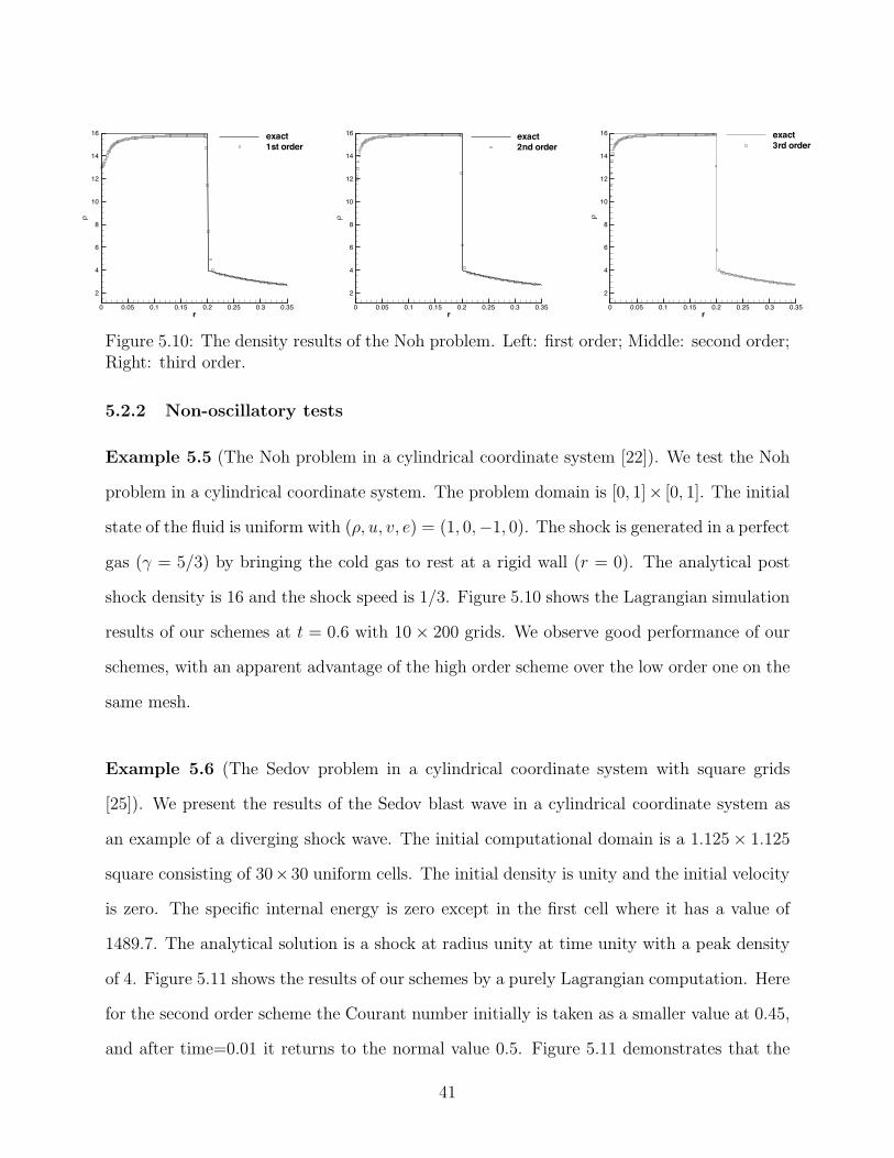
Figure 5.10: The density results of the Noh problem. Left: first order; Middle: second order;Right: third order.

5.2.2 Non-oscillatory tests

Example 5.5 (The Noh problem in a cylindrical coordinate system [22]). We test the Noh

problem in a cylindrical coordinate system. The problem domain is [0, 1]× [0, 1]. The initial

state of the fluid is uniform with (ρ, u, v, e) = (1, 0,−1, 0). The shock is generated in a perfect

gas (γ = 5/3) by bringing the cold gas to rest at a rigid wall (r = 0). The analytical post

shock density is 16 and the shock speed is 1/3. Figure 5.10 shows the Lagrangian simulation

results of our schemes at t = 0.6 with 10 × 200 grids. We observe good performance of our

schemes, with an apparent advantage of the high order scheme over the low order one on the

same mesh.

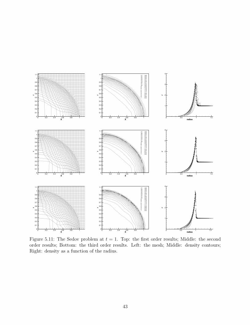
Example 5.6 (The Sedov problem in a cylindrical coordinate system with square grids

[25]). We present the results of the Sedov blast wave in a cylindrical coordinate system as

an example of a diverging shock wave. The initial computational domain is a 1.125 × 1.125

square consisting of 30×30 uniform cells. The initial density is unity and the initial velocity

is zero. The specific internal energy is zero except in the first cell where it has a value of

1489.7. The analytical solution is a shock at radius unity at time unity with a peak density

of 4. Figure 5.11 shows the results of our schemes by a purely Lagrangian computation. Here

for the second order scheme the Courant number initially is taken as a smaller value at 0.45,

and after time=0.01 it returns to the normal value 0.5. Figure 5.11 demonstrates that the

41

Lagrangian schemes also can produce good results for the Sedov problem in the cylindrical

coordinates.

Example 5.7 (Interaction of a shock with longitudinal vortex [11]). The computational

domain is [−8, 4] × [0, 5]. At t = 0, there is a mean flow with a stationary shock at x = 0,

that is

(ρ, p, ux, ur, u#) =

(+)

+*

(ρ1, p1, ux,1, ur,1, u#,1) = (1, 1, γ1/2M1, 0, 0), x < 0

(ρ2, p2, ux,2, ur,2, u#,2) = [ ($+1)M21

2+M21 ($−1)

, 2$M21−($−1)($+1) , M2

0γ p2

!2, 0, 0], x > 0

where M1 is the Mach number at the upstream of the shock (x < 0) and M2 = 2+M21 ($−1)

2$M21−($−1)

is the Mach number at the downstream of the shock (x > 0).

Next, we superimpose an isentropic vortex with its axis along r = 0 on the upstream of

the mean flow. The perturbation of azimuthal velocity u′# and temperature T

′associated

with the vortex are given by

u′

# =εr

2πe0.5(1−r2), T

′= −(γ − 1)ε2

8γπ2r20

e1−r2(5.1)

where r0 is the vortex core radius and ε is a non-dimensional circulation at r = 1. The axial

and radial velocities u′x, u

′r are zero. With no perturbation of the entropy S = log(p/ρ$) of

the original mean flow, the final perturbed flow at x < 0 is as follows

ρ =

1T1 + T

′

p1/ρ$1

21/($−1)

, p = (T1 + T′)ρ, ux = ux,1, ur = 0, u# = u

′

#

where T1 = p1/ρ1. In this test, we set M1 = 2, ε = 7 and r0 = 1. The supersonic inflow,

characteristic, symmetry and Neumann conditions are used at the left, right, bottom and

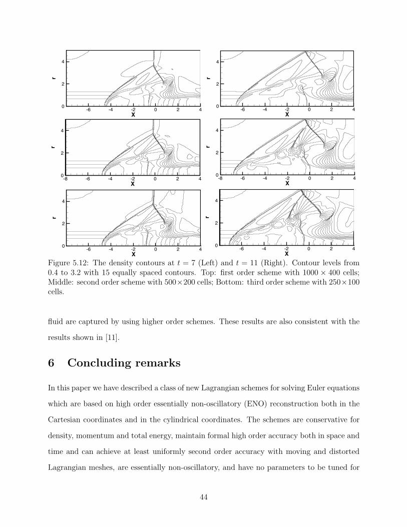
upper boundaries respectively. The initial grid is uniform. After every three Lagrangian

time steps, we take the rezoning and remapping steps to return the Lagrangian grid to the

initial grid. The density results at two typical times of our schemes are given in Figures

5.12. From these figures we observe that the resolution of high order schemes on coarser

meshes are comparable to that of low order schemes on finer meshes, and more details of the

42

X

r

0 0.2 0.4 0.6 0.8 10

0.1

0.2

0.3

0.4

0.5

0.6

0.7

0.8

0.9

1

1.1

1

1

2

2

3

3

4

4

5

5

5

5

5

6

6

6

6

6

7

7

7

7

7

8

8

8

8

8

9

9

9

9

9

10

10

10

10

10

11

11

11

11

11

12

12

12

12

13

13

13

X

r

0 0.2 0.4 0.6 0.8 10

0.1

0.2

0.3

0.4

0.5

0.6

0.7

0.8

0.9

1

1.1 17 3.816 3.615 3.414 3.113 2.912 2.711 2.510 2.29 2.08 1.87 1.66 1.35 1.14 0.93 0.72 0.41 0.2

radius

!

0 0.5 1 1.5

1

2

3

4

X

r

0 0.2 0.4 0.6 0.8 10

0.1

0.2

0.3

0.4

0.5

0.6

0.7

0.8

0.9

1

1.1

1

2 3

3

4

4

5

5

5

5

6

6

6

6

6

7

7

7

7

7

7

8

8

8

8

9

9

9

9

9

10

10

10

10

10

10

11

11

11

11

12

12

12

12

12

13

13

13

13

14

14

14

14

X

r

0 0.2 0.4 0.6 0.8 10

0.1

0.2

0.3

0.4

0.5

0.6

0.7

0.8

0.9

1

1.1 17 3.816 3.615 3.414 3.113 2.912 2.711 2.510 2.29 2.08 1.87 1.66 1.35 1.14 0.93 0.72 0.41 0.2

radius

!

0 0.5 1 1.5

1

2

3

4

X

r

0 0.2 0.4 0.6 0.8 10

0.1

0.2

0.3

0.4

0.5

0.6

0.7

0.8

0.9

1

1.1

1

1

2

2

3

3

4

4

5

5

5

5

5

6

6

6

6

6

6

7

7

7

7

7

8

8

8

8

8

9

9

9

9

9

10

10

10

10

11

11

11

11

11

12

12

12

12

12

13

13

13

13

13

14

14

14

14

14

15

15

X

r

0 0.2 0.4 0.6 0.8 10

0.1

0.2

0.3

0.4

0.5

0.6

0.7

0.8

0.9

1

1.1 17 3.816 3.615 3.314 3.113 2.912 2.711 2.510 2.29 2.08 1.87 1.56 1.35 1.14 0.93 0.62 0.41 0.2

radius

!

0 0.5 1 1.5

1

2

3

4

Figure 5.11: The Sedov problem at t = 1. Top: the first order results; Middle: the secondorder results; Bottom: the third order results. Left: the mesh; Middle: density contours;Right: density as a function of the radius.

43

X

r

-6 -4 -2 0 2 40

2

4

X

r

-6 -4 -2 0 2 40

2

4

X

r

-8 -6 -4 -2 0 2 40

2

4

X

r

-8 -6 -4 -2 0 2 40

2

4

X

r

-6 -4 -2 0 2 40

2

4

X

r

-6 -4 -2 0 2 40

2

4

Figure 5.12: The density contours at t = 7 (Left) and t = 11 (Right). Contour levels from0.4 to 3.2 with 15 equally spaced contours. Top: first order scheme with 1000 × 400 cells;Middle: second order scheme with 500×200 cells; Bottom: third order scheme with 250×100cells.

fluid are captured by using higher order schemes. These results are also consistent with the

results shown in [11].

6 Concluding remarks

In this paper we have described a class of new Lagrangian schemes for solving Euler equations

which are based on high order essentially non-oscillatory (ENO) reconstruction both in the

Cartesian coordinates and in the cylindrical coordinates. The schemes are conservative for

density, momentum and total energy, maintain formal high order accuracy both in space and

time and can achieve at least uniformly second order accuracy with moving and distorted

Lagrangian meshes, are essentially non-oscillatory, and have no parameters to be tuned for

44

individual test cases. It can be extended to higher order accuracy by using curved meshes.

Comparing with many current Lagrangian schemes, our ENO schemes overcome some of

their disadvantages such as non-conservativity of momentum and total energy, low accuracy,

and the existence of parameters which must be adjusted for individual test cases. One

dimensional and two dimensional examples in the Cartesian as well as cylindrical coordinates

have been presented which demonstrate the good performance of the schemes both in purely

Lagrangian and in ALE calculations. Although we have only performed tests on quadrilateral

grids, the strategy can be used on any polygon grid such as triangles. The investigation and

improvement of these high order schemes in multi dimensions in terms of accuracy, resolution,

and desirable properties such as symmetry preservation, constitute future work.

References

[1] R. Abgrall, On essentially non-oscillatory schemes on unstructured meshes: analysis

and implementation, Journal of Computational Physics, 114, 1994, 45-58.

[2] R. Abgrall, J. Breil, P.H. Maire and J. Ovadia, A cell-centered Lagrangian scheme for

two-dimensional compressible flow problems, SIAM Journal on Scientific Computing, to

appear.

[3] D.J. Benson, Computational methods in Lagrangian and Eulerian hydrocodes, Computer

Methods in Applied Mechanics and Engineering, 99, 1992, 235-394.

[4] D.J. Benson, Momentum advection on a staggered mesh, Journal of Computational

Physics, 100, 1992, 143-162.

[5] J.C. Campbell and M.J. Shashkov, A tensor artificial viscosity using a mimetic finite

difference algorithm, Journal of Computational Physics, 172, 2001, 739-765.

45

[6] E.J. Caramana, D.E. Burton, M.J. Shashkov and P.P. Whalen, The construction of

compatible hydrodynamics algorithms utilizing conservation of total energy, Journal of

Computational Physics, 146, 1998, 227-262.

[7] J. Cheng and C.-W. Shu, A high order accurate conservative remapping method on

staggered meshes, Applied Numerical Mathematics, to appear.

[8] B. Despres and C. Mazeran, Lagrangian gas dynamics in two dimensions and lagrangian

systems, Archive for Rational Mechanics and Analysis, 178, 2005, 327-372.

[9] J.K. Dukowicz, M.C. Cline and F.L. Addessio, A general topology Godunov method,

Journal of Computational Physics, 82, 1989, 29-63.

[10] J.K. Dukowicz and B.J.A. Meltz, Vorticity errors in multidimensional Lagrangian codes,

Journal of Computational Physics, 99, 1992, 115-134.

[11] G. Erlebacher, M.Y. Hussaini and C.-W. Shu, Interaction of a shock with a longitudinal

vortex, Journal of Fluid Mechanics, 337, 1997, 129-153.

[12] A. Harten, B. Engquist, S. Osher and S.R. Chakravarthy, Uniformly high order accurate

essentially non-oscillatory schemes, III, Journal of Computational Physics, 71, 1987,

231-303.

[13] A. Harten and S. Osher, Uniformly high-order accurate nonoscillatory schemes I, SIAM

Journal on Numerical Analysis, 24, 1987, 279-309.

[14] C. Hirt, A. Amsden and J. Cook, An arbitrary Lagrangian-Eulerian computing method

for all flow speeds, Journal of Computational Physics, 14, 1974, 227-253.

[15] G. Jiang and C.-W. Shu, Efficient implementation of weighted ENO schemes, Journal

of Computational Physics, 126, 1996, 202-228.

46

[16] D.S. Kershaw, M.K. Prasad, M.J. Shaw and J.L. Milovich, 3D unstructured mesh ALE

hydrodynamics with the upwind discontinuous finite element method, Computer Methods

in Applied Mechanics and Engineering, 158, 1998, 81-116.

[17] B. Koobus and C. Farhat, Second-order time-accurate and geometrically conservative

implicit schemes for flow computations on unstructured dynamic meshes, Computer

Methods in Applied Mechanics and Engineering, 170, 1999, 103-129.

[18] R. Loubere and M.J. Shashkov, A subcell remapping method on staggered polygonal

grids for arbitrary-Lagrangian-Eulerian methods, Journal of Computational Physics,

209, 2005, 105-138.

[19] H. Luo, J.D. Baum and R. Lohner, On the computation of multi-material flows using

ALE formulation, Journal of Computational Physics, 194, 2004, 304-328.

[20] L.G. Margolin, Introduction to “An arbitrary Lagrangian-Eulerian computing method

for all flow speeds”, Journal of Computational Physics, 135, 1997, 198-202.

[21] J. von Neumann and R.D. Richtmyer, A method for the calculation of hydrodynamics

shocks, Journal of Applied Physics, 21, 1950, 232-237.

[22] W.F. Noh, Errors for calculations of strong shocks using an artificial viscosity and an

artificial heat flux, Journal of Computational Physics, 72, 1987, 78-120.

[23] J.S. Peery and D.E. Carroll, Multi-material ALE methods in unstructured grids, Com-

puter Methods in Applied Mechanics and Engineering, 187, 2000, 591-619.

[24] A. Rogerson and E. Meiberg, A numerical study of the convergence properties of ENO

schemes, Journal of Scientific Computing, 5, 1990, 151-167.

[25] L.I. Sedov, Similarity and Dimensional Methods in Mechanics, Academic Press, New

York, 1959.

47

[26] C.-W. Shu, Numerical experiments on the accuracy of ENO and modified ENO schemes,

Journal of Scientific Computing, 5, 1990, 127-149.

[27] C.-W. Shu, Preface to the republication of “Uniformly high order essentially non-

oscillatory schemes, III”, by Harten, Engquist, Osher, and Chakravarthy, Journal of

Computational Physics, 131, 1997, 1-2.

[28] C.-W. Shu, Essentially non-oscillatory and weighted essentially non-oscillatory schemes

for hyperbolic conservation laws, in Advanced Numerical Approximation of Nonlinear

Hyperbolic Equations, B. Cockburn, C. Johnson, C.-W. Shu and E. Tadmor (Editor:

A. Quarteroni), Lecture Notes in Mathematics, volume 1697, Springer, Berlin, 1998,

pp.325-432.

[29] C.-W. Shu and S. Osher, Efficient implementation of essentially non-oscillatory shock-

capturing schemes, Journal of Computational Physics, 77, 1988, 439-471.

[30] C.-W. Shu and S. Osher, Efficient implementation of essentially non-oscillatory shock

capturing schemes II, Journal of Computational Physics, 83, 1989, 32-78.

[31] C.-W. Shu, T.A. Zang, G. Erlebacher, D. Whitaker and S. Osher, High-order ENO

schemes applied to two- and three-dimensional compressible flow, Applied Numerical

Mathematics, 9, 1992, 45-71.

[32] R.W. Smith, AUSM(ALE): a geometrically conservative arbitrary Lagrangian-Eulerian

flux splitting scheme, Journal of Computational Physics, 150, 1999, 268-286.

[33] H.Z. Tang and T.T. Liu, A note on the conservative schemes for the Euler equations,

Journal of Computational Physics, 218, 2006, 451-459.

[34] E.F. Toro, Riemann Solvers and Numerical Methods for Fluid Dynamics, Springer-

Verlag, Berlin, 1999.

48

[35] P.R. Woodward and P. Colella, The numerical simulation of two-dimensional fluid flow

with strong shocks, Journal of Computational Physics, 54, 1984, 115-173.

49