A HAMILTONIAN VORTICITY-DILATATION FORMULATION OF … · vorticity and dilatation, and to formulate the Euler equations in terms of these new variables. Section 4 deals with the Hamiltonian

M

em

ora

nd

um

20

15

(S

ep

tem

be

r 2

01

3).

IS

SN

18

74

−4

85

0. A

vaila

ble

fro

m: h

ttp

://w

ww

.ma

th.u

twe

nte

.nl/p

ub

lica

tion

s D

ep

art

me

nt o

f A

pp

lied

Ma

the

ma

tics,

Un

ive

rsity

of T

we

nte

, E

nsc

he

de

, T

he

Ne

the

rla

nd

s

A HAMILTONIAN VORTICITY-DILATATION FORMULATION OF

THE COMPRESSIBLE EULER EQUATIONS

MONIKA POLNER

Bolyai Institute,

University of Szeged, Aradi vertanuk tere 1, 6720 Szeged, Hungary

[email protected]

J.J.W. VAN DER VEGT

Department of Applied Mathematics,

University of Twente, P.O. Box 217, 7500 AE, Enschede, The Netherlands

[email protected]

Using the Hodge decomposition on bounded domains the compressible Euler equations

of gas dynamics are reformulated using a density weighted vorticity and dilatation as

primary variables, together with the entropy and density. This formulation is an extension

to compressible flows of the well-known vorticity-stream function formulation of the

incompressible Euler equations. The Hamiltonian and associated Poisson bracket for

this new formulation of the compressible Euler equations are derived and extensive use

is made of differential forms to highlight the mathematical structure of the equations.

In order to deal with domains with boundaries also the Stokes-Dirac structure and the

port-Hamiltonian formulation of the Euler equations in density weighted vorticity and

dilatation variables are obtained.

Keywords: Compressible Euler equations; Hamiltonian formulation; de Rham complex;

Hodge decomposition; Stokes-Dirac structures, vorticity, dilatation.

AMS Subject Classification: 37K05, 58A14, 58J10, 35Q31, 76N15, 93C20, 65N30.

1. Introduction

The dynamics of an inviscid compressible gas is described by the compressible Euler

equations, together with an equation of state. The compressible Euler equations

have been extensively used to model many different types of compressible flows,

since in many applications the effects of viscosity are small or can be neglected.

This has motivated over the years extensive theoretical and numerical studies of

the compressible Euler equations. The Euler equations for a compressible, inviscid

and non-isentropic gas in a domain Ω ⊆ R3 are defined as

ρt = −∇ · (ρu), (1.1)

ut = −u · ∇u−1

ρ∇p, (1.2)

st = −u · ∇s, (1.3)

1

2 Polner and Van der Vegt

with u = u(x, t) ∈ R3 the fluid velocity, ρ = ρ(x, t) ∈ R

+ the mass density and

s(x, t) ∈ R the entropy of the fluid, which is conserved along streamlines. The

spatial coordinates are x ∈ Ω and time t and the subscript means differentiation

with respect to time. The pressure p(x, t) is given by an equation of state

p = ρ2∂U

∂ρ(ρ, s), (1.4)

where U(ρ, s) is the internal energy function that depends on the density ρ and

the entropy s of the fluid. The compressible Euler equations have a rich mathe-

matical structure,12 and can be represented as an infinite dimensional Hamiltonian

system,10,11. Depending on the field of interest, various types of variables have been

used to define the Euler equations, e.g. conservative, primitive and entropy variables,12. The conservative variable formulation is for instance a good starting point for

numerical discretizations that can capture flow discontinuities,8 such as shocks and

contact waves, whereas the primitive and entropy variables are frequently used in

theoretical studies.

In many flows vorticity is, however, the primary variable of interest. Historically,

the Kelvin circulation theorem and Helmholtz theorems on vortex filaments have

played an important role in describing incompressible flows, in particular the im-

portance of vortical structures. This has motivated the use of vorticity as primary

variable in theoretical studies of incompressible flows, see e.g.1,10, and the develop-

ment of vortex methods to compute incompressible vortex dominated flows,6.

The use of vorticity as primary variable is, however, not very common for com-

pressible flows. This is partly due to the fact that the equations describing the

evolution of vorticity in a compressible flow are considerably more complicated

than those for incompressible flows. Nevertheless, vorticity is also very important

in many compressible flows. A better insight into the role of vorticity, and also di-

latation to account for compressibility effects, is not only of theoretical importance,

but also relevant for the development of numerical discretizations that can compute

these quantities with high accuracy.

In this article we will present a vorticity-dilatation formulation of the compress-

ible Euler equations. Special attention will be given to the Hamiltonian formulation

of the compressible Euler equations in terms of the density weighted vorticity and

dilatation variables on domains with boundaries. This formulation is an extension

to compressible flows of the well-known vorticity-stream function formulation of

the incompressible Euler equations,1,10. An important theoretical tool in this anal-

ysis is the Hodge decomposition on bounded domains,15. Since bounded domains

are crucial in many applications we also consider the Stokes-Dirac structure of the

compressible Euler equations. This results in a port-Hamiltonian formulation,14

of the compressible Euler equations in terms of the vorticity-dilatation variables,

which clearly identifies the flows and efforts entering and leaving the domain. An

important feature of our presentation is that we extensively use the language of dif-

ferential forms. Apart from being a natural way to describe the underlying mathe-

A Hamiltonian vorticity-dilatation formulation of the compressible Euler equations 3

matical structure it is also important for our long term objective, viz. the derivation

of finite element discretizations that preserve the mathematical structure as much

as possible. A nice way to achieve this is by using discrete differential forms and

exterior calculus, as highlighted in Ref. 2, 3.

The outline of this article is as follows. In the introductory Section 2 we sum-

marize the main techniques that we will use in our analysis. A crucial element is

the use of the Hodge decomposition on bounded domains, which we briefly discuss

in Section 2.2. This analysis is based on the concept of Hilbert complexes, which

we summarize in Section 2.1. The Hodge Laplacian problem is discussed in Section

2.3. Here we show how to deal with inhomogeneous boundary conditions, which is

of great importance for our applications. These results will be used in Section 3 to

define via the Hodge decomposition a new set of variables, viz., the density weighted

vorticity and dilatation, and to formulate the Euler equations in terms of these new

variables. Section 4 deals with the Hamiltonian formulation of the Euler equations

using the density weighted vorticity and dilatation, together with the density and

entropy, as primary variables. The Poisson bracket for the Euler equations in these

variables is derived in Section 5. In order to account for bounded domains we ex-

tend the results obtained for the Hamiltonian formulation in Sections 4 and 5 to the

port-Hamiltonian framework in Section 6. First, we extend in Section 6.1 the Stokes-

Dirac structure for the isentropic compressible Euler equations presented in Ref. 13

to the non-isentropic Euler equations. Next, we derive the Stokes-Dirac structure

for the compressible Euler equations in the vorticity-dilatation formulation in Sec-

tion 6.2 and use this in Section 6.3 to obtain a port-Hamiltonian formulation of the

compressible Euler equations in vorticity-dilatation variables. Finally, in Section 7

we finish with some conclusions.

2. Preliminaries

This preliminary section is devoted to summarize the main concepts and techniques

that we use throughout this paper in our analysis.

2.1. Review of Hilbert complexes

In this section we discuss the abstract framework of Hilbert complexes, which is the

basis of the exterior calculus in Arnold, Falk and Winther,3 and to which we refer

for a detailed presentation. We also refer to Bruning and Lesch,5 for a functional

analytic treatment of Hilbert complexes.

Definition 2.1. A Hilbert complex (W,d) consists of a sequence of Hilbert spaces

W k, along with closed, densely-defined linear operators dk : W k →W k+1, possibly

unbounded, such that the range of dk is contained in the domain of dk+1 and

dk+1 dk = 0 for each k.

A Hilbert complex is bounded if, for each k, dk is a bounded linear operator

from W k to W k+1 and it is closed if for each k, the range of dk is closed in W k+1.


Definition 2.2. Given a Hilbert complex (W, d), a domain complex (V, d) consists

of domains D(dk) = V k ⊂W k, endowed with the graph inner product

〈u, v〉V k = 〈u, v〉Wk +⟨dku, dkv

⟩

Wk+1 .

Remark 2.1. Since dk is a closed map, each V k is closed with respect to the norm

induced by the graph inner product. From the Closed Graph Theorem, it follows

that dk is a bounded operator from V k to V k+1. Hence, (V, d) is a bounded Hilbert

complex. The domain complex is closed if and only if the original complex (W, d)

is.

Definition 2.3. Given a Hilbert complex (W, d), the space of k-cocycles is the

null space Zk = ker dk, the space of k-coboundaries is the image Bk = dk−1V k−1,

the kth harmonic space is the intersection Hk = Zk ∩Bk⊥W , and the kth reduced

cohomology space is the quotient Zk/Bk. When Bk is closed, Zk/Bk is called the

kth cohomology space.

Remark 2.2. The harmonic space Hk is isomorphic to the reduced cohomology

space Zk/Bk. For a closed complex, this is identical to the homology space Zk/Bk,

since Bk is closed for each k.

Definition 2.4. Given a Hilbert complex (W,d), the dual complex (W ∗, d∗) con-

sists of the spaces W ∗k = W k, and adjoint operators d∗k = (dk−1)∗ : V ∗

k ⊂ W ∗k →

V ∗k−1 ⊂W ∗

k−1. The domain of d∗k is denoted by V ∗k , which is dense in W k.

Definition 2.5. We can define the k-cycles Z∗k = ker d∗k = Bk⊥W and k-boundaries

B∗k = d∗k+1V

∗k .

2.2. The L2-de Rham complex and Hodge decomposition

The basic example of a Hilbert complex is the L2-de Rham complex of differential

forms. Let Ω ⊆ Rn be an n-dimensional oriented manifold with Lipschitz boundary

∂Ω, representing the space of spatial variables. Assume that there is a Riemannian

metric ≪,≫ on Ω. We denote by Λk(Ω) the space of smooth differential k-forms

on Ω, d is the exterior derivative operator, taking differential k-forms on the do-

main Ω to differential (k + 1)-forms, δ represents the codifferential operator and ⋆

the Hodge star operator associated to the Riemannian metric ≪,≫ . The opera-

tions grad, curl, div,×, · from vector analysis can be identified with operations on

differential forms, see e.g. Ref. 7.

For the domain Ω and non-negative integer k, let L2Λk = L2Λk(Ω) denote the

Hilbert space of differential k-forms on Ω with coefficients in L2. The inner product

in L2Λk is defined as

〈ω, η〉L2Λk =

∫

Ω

ω ∧ ⋆η =

∫

Ω

≪ ω, η ≫ vΩ =

∫

Ω

⋆(ω ∧ ⋆η)vΩ, ω, η ∈ L2Λk, (2.1)

where vΩ is the Riemannian volume form. When Ω is omitted from L2Λk in the inner

product (2.1), then the integral is always over Ω. The exterior derivative d = dk may


be viewed as an unbounded operator from L2Λk to L2Λk+1. Its domain, denoted

by HΛk(Ω), is the space of differential forms in L2Λk(Ω) with the weak derivative

in L2Λk+1(Ω), that is

D(d) = HΛk(Ω) = ω ∈ L2Λk(Ω) | dω ∈ L2Λk+1(Ω),

which is a Hilbert space with the inner product

〈ω, η〉HΛk = 〈ω, η〉L2Λk + 〈dω, dη〉L2Λk+1 .

For an oriented Riemannian manifold Ω ⊆ R3, the L2 de Rham complex is

0→ L2Λ0(Ω)d−→ L2Λ1(Ω)

d−→ L2Λ2(Ω)d−→ L2Λ3(Ω)→ 0. (2.2)

Note that d is a bounded map from HΛk(Ω) to L2Λk+1(Ω) and D(d) = HΛk(Ω) is

densely-defined in L2Λk(Ω). Since HΛk(Ω) is complete with the graph norm, d is

a closed operator (equivalent statement to the Closed Graph Theorem). Thus, the

the L2 de Rham domain complex for Ω ⊆ R3 is

0→ HΛ0(Ω)d−→ HΛ1(Ω)

d−→ HΛ2(Ω)d−→ HΛ3(Ω)→ 0. (2.3)

The coderivative operator δ : L2Λk(Ω) 7→ L2Λk−1(Ω) is defined as

δω = (−1)n(k+1)+1 ⋆ d ⋆ ω, ω ∈ L2Λk(Ω). (2.4)

Since we assumed that Ω has Lipschitz boundary, the trace theorem holds and the

trace operator tr∂Ω = tr maps HΛk(Ω) boundedly into an appropriate Sobolev

space on ∂Ω. We denote the space HΛk(Ω) with vanishing trace as

HΛk(Ω) = ω ∈ HΛk(Ω) | tr ω = 0. (2.5)

In analogy with HΛk(Ω), we can define the space

H∗Λk(Ω) =ω ∈ L2Λk(Ω) | δω ∈ L2Λk−1(Ω)

. (2.6)

Since H∗Λk(Ω) = ⋆HΛn−k(Ω), for ω ∈ H∗Λk(Ω), the quantity tr(⋆ω) is well de-

fined, and we have

H∗Λk(Ω) = ⋆

HΛn−k(Ω) = ω ∈ H∗Λk(Ω) | tr(⋆ω) = 0. (2.7)

The adjoint d∗ = d∗k of dk−1 has domain D(d∗) =H∗Λk(Ω) and coincides with the

operator δ defined in (2.4), (see Ref. 3). Hence, the dual complex of (2.3) is

0←H∗Λ0(Ω)

δ←−H∗Λ1(Ω)

δ←−H∗Λ2(Ω)

δ←−H∗Λ3(Ω)← 0. (2.8)

The integration by parts formula also holds

〈dω, η〉 = 〈ω, δη〉+∫

∂Ω

trω ∧ tr(⋆η), ω ∈ Λk−1(Ω), η ∈ Λk(Ω), (2.9)

and we have

〈dω, η〉 = 〈ω, δη〉 , ω ∈ HΛk−1(Ω), η ∈H∗Λk(Ω). (2.10)


Since the L2-de Rham complexes (2.2) and (2.3) are closed Hilbert complexes, the

Hodge decomposition of L2Λk and HΛk are:

L2Λk = Bk ⊕ Hk ⊕B∗

k, (2.11)

HΛk = Bk ⊕ Hk ⊕ Zk⊥, (2.12)

whereB∗

k = δω | ω ∈H∗Λk+1(Ω), and Zk⊥ = HΛk ∩

B∗

k denotes the orthogonal

complement of Zk in HΛk. The space of harmonic forms, both for the original

complex and the dual complex, is

Hk = ω ∈ HΛk(Ω) ∩H∗Λk(Ω) | dω = 0, δω = 0. (2.13)

Problems with essential boundary conditions are important for applications. This

is why we briefly review the de Rham complex with essential boundary conditions.

Take as domain of the exterior derivative dk the spaceHΛk(Ω). The de Rham

complex with homogeneous boundary conditions on Ω ⊂ R3 is

0→HΛ0(Ω)

d−→HΛ1(Ω)

d−→HΛ2(Ω)

d−→HΛ3(Ω)→ 0. (2.14)

From (2.9), we obtain that

〈dω, η〉 = 〈ω, δη〉 , ω ∈HΛk−1(Ω), η ∈ H∗Λk(Ω). (2.15)

Hence, the adjoint d∗ of the exterior derivative with domainHΛk(Ω) has domain

H∗Λk(Ω) and coincides with the operator δ. Finally, the second Hodge decomposi-

tion of L2Λk and ofHΛk follow immediately:

L2Λk =B

k ⊕H

k ⊕B∗k, (2.16)

HΛk =

B

k ⊕H

k ⊕ Zk⊥, (2.17)

whereB

k = dHΛk−1(Ω), Zk⊥ =

HΛk ∩B∗

k and the space of harmonic forms is

H

k = ω ∈HΛk(Ω) ∩H∗Λk(Ω) | dω = 0, δω = 0. (2.18)

2.3. The Hodge Laplacian problem

In this section we first review the Hodge Laplacian problem with homogeneous

natural and essential boundary conditions. The main result of this section is to

show how to deal with inhomogeneous boundary conditions, which are crucial for

applications.


2.3.1. The Hodge Laplacian problem with homogeneous natural boundary

conditions

Given the Hilbert complex (2.3) and its dual complex (2.8), the Hodge Laplacian

operator applied to a k-form is an unbounded operator Lk = dk−1d∗k + d∗k+1dk :

D(Lk) ⊂ L2Λk → L2Λk, with domain (see Ref. 3)

D(Lk) = u ∈ HΛk ∩H∗Λk | dku ∈

H∗ Λk+1, d∗ku ∈ HΛk−1. (2.19)

In the following, we will not use the subscripts and superscripts k of the operators

when they are clear from the context and use d∗ = δ.

For any f ∈ L2Λk, there exists a unique solution u = Kkf ∈ D(Lk) satisfying

Lku = f (mod H), u ⊥ H, (2.20)

with Kk the solution operator, see Ref. 3. The solution u satisfies the Hodge Lapla-

cian (homogeneous) boundary value problem

(dδ + δd)u = f − PHf in Ω, tr(⋆u) = 0, tr(⋆du) = 0 on ∂Ω, (2.21)

where PHf is the orthogonal projection of f into H, with the condition u ⊥ H

required for uniqueness of the solution. The boundary conditions in (2.21) are both

natural in the mixed variational formulation of the Hodge Laplacian problem, as

discussed in Ref 3.

The Hodge Laplacian problem is closely related to the Hodge decomposition in

the following way. Since dδu ∈ Bk and δdu ∈ B∗k, the differential equation in (2.21),

or equivalently f = dδu+ δdu+ α, α ∈ Hk, is exactly the Hodge decomposition of

f ∈ L2Λk(Ω). If we restrict f to an element of Bk or B∗k, we obtain two problems

that are important for our applications (see also Ref. 3).

The B problem. If f ∈ Bk, then u ∈ Kkf satisfies dδu = f, u ⊥Z∗k, where

Z∗k = ω ∈

H∗Λk(Ω) | δω = 0. It also follows that the solution u ∈ Bk. To see

this, consider u ∈ D(Lk) and the Hodge decomposition u = uB + uH + u⊥, where

uB ∈ Bk, uH ∈ Hk and u⊥ ∈ B∗k ∩HΛk. Then,

Lku = dδuB + δdu⊥ = f.

If f ∈ Bk, then u = uB, hence u ∈ Bk. Then, duB = 0 since d2 = 0, and since

Bk =Z∗k⊥, it follows that u ⊥

Z∗k is also satisfied and u solves uniquely the Hodge

Laplacian boundary value problem, see Ref. 3,

dδu = f, du = 0, u ⊥Z∗k in Ω (2.22)

tr(⋆u) = 0, on ∂Ω. (2.23)

The B∗ problem. If f ∈ B∗k, then u = Kkf satisfies δdu = f, with u ⊥ Zk.

Similarly as for the B problem, it can be shown that the solution u ∈ B∗k. Consider

u ∈ D(Lk) and the Hodge decomposition u = uB + uH + u⊥. Then,

Lku = dδuB + δdu⊥ = f.


If f ∈ B∗k, then u = u⊥, hence u ∈ B∗

k. Therefore, δu⊥ = 0 and u ⊥ Zk. Conse-

quently, u solves uniquely the Hodge Laplacian boundary value problem

δdu = f, δu = 0, u ⊥ Zk in Ω (2.24)

tr(⋆du) = 0, on ∂Ω. (2.25)

2.3.2. The Hodge Laplacian problem with homogeneous essential boundary

conditions

Considering now the Hilbert complex with (homogeneous) boundary conditions

(2.14) and its dual complex, the Hodge Laplacian problem with essential boundary

conditions is

Lku = dδu+ δdu = f (modH), in Ω (2.26)

tr(δu) = 0, tru = 0 on ∂Ω, (2.27)

with the condition u ⊥H, which has a unique solution, u = Kkf. Both boundary

conditions in (2.27) are essential in the mixed variational formulation of the Hodge

Laplacian problem (see Ref. 3). Here the domain of the Laplacian is

D(Lk) = u ∈HΛk ∩H∗Λk | du ∈ H∗Λk+1, δu ∈

HΛk−1. (2.28)

We can briefly formulate the B and B∗ problems as follows.

The B problem. If f ∈B

k, then then u ∈ Kkf ∈B

k satisfies dδu = f, u ⊥ Z∗k.

Then u solves uniquely the B problem

dδu = f, du = 0, u ⊥ Z∗k in Ω (2.29)

tr(δu) = 0, on ∂Ω. (2.30)

The B∗ problem. If f ∈ B∗k, then u = Kkf satisfies δdu = f, with u ⊥ Zk.

Similarly, u solves uniquely

δdu = f, δu = 0, u ⊥ Zk in Ω (2.31)

tr(u) = 0, on ∂Ω. (2.32)

The next section shows how to transform the inhomogeneous Hodge Laplacian

boundary value problem into a homogeneous one.

2.3.3. The Hodge Laplacian with inhomogeneous essential boundary

conditions

Consider the case when the essential boundary conditions are inhomogeneous, that

is, the boundary value problem

Lku = dδu+ δdu = f in Ω (2.33)

tru = rb, tr(δu) = rN on ∂Ω, (2.34)


with the condition

〈f, α〉 =∫

∂Ω

rN ∧ tr(⋆α), ∀α ∈H

k. (2.35)

Here the domain of the Hodge Laplacian operator is

DDk =

u ∈ HΛk ∩H∗Λk | du ∈ H∗Λk+1, δu ∈ HΛk−1,

tru = rb ∈ H1/2Λk(∂Ω), tr(δu) = rN ∈ H1/2Λk−1(∂Ω)

. (2.36)

This problem has a solution, which is unique up to a harmonic form α ∈Hk. Fol-

lowing the idea of Schwarz in Ref. 15, the inhomogeneous boundary value problem

can be transformed to a homogeneous problem in the following way. For a given

rb ∈ H1/2Λk(∂Ω), using a bounded, linear trace lifting operator (see Ref. 4, 2, 15),

we can find η ∈ H1Λk(Ω), such that tr η = rb. The Hodge decomposition of η

η = dφη + δβη + αη, dφη ∈B

k, δβη ∈ B∗k, α ∈

H

k

means for the trace that

tr η = d(trφη) + tr(δβη) + trαη = tr(δβη),

viz. the components dφη and αη of the extension η do not contribute to the tr η.

Hence, we can construct η = δβη. Then, Lkη = δdδβη and it can be easily shown

that 〈Lkη, α〉 = 0 for all α ∈Hk.

On the other hand, given rN ∈ H1/2Λk−1(∂Ω), the extension result of Lemma

3.3.2 in Ref. 15, guarantees the existence of η ∈ H1ΛkΩ, such that

tr η = 0 and tr(δη) = rN .

Take u = u − η − η. Then, Lku = f − Lkη − Lkη =: f , tr u = 0, tr(δu) = 0 and

using the condition (2.35), we can show that f ⊥Hk. Hence, u is the solution of

the homogeneous boundary value problem (2.26)-(2.27) with the right hand side f .

2.3.4. The Hodge Laplacian with inhomogeneous natural boundary conditions

Consider the Hodge Laplacian operator Lk = dδ + δd : D(Lk) ⊂ L2Λk → L2Λk,

with domain

DNk =

u ∈ HΛk ∩H∗Λk | du ∈ H∗Λk+1, δu ∈ HΛk−1,

tr(⋆u) = gb ∈ H−1/2Λn−k(∂Ω), tr(⋆du) = gN ∈ H−1/2Λn−k−1(∂Ω)

.

(2.37)

Our aim is to transform the inhomogeneous boundary value problem

(dδ + δd)u = f in Ω (2.38)

tr(⋆u) = gb, tr(⋆du) = gN on ∂Ω, (2.39)


with the condition

〈f, α〉 = −∫

∂Ω

trα ∧ gN ∀α ∈ Hk, (2.40)

and the side condition for uniqueness u ⊥ Hk, into the Hodge Laplacian homo-

geneous boundary value problem (2.21). This can be considered as the dual of

the problem with inhomogeneous essential boundary conditions, treated in Section

2.3.3. For completeness, we briefly summarize the steps of the construction.

For gb ∈ H−1/2Λn−k(∂Ω) we can find τ ∈ H∗Λk(Ω) with tr(⋆τ) = gb. Note here

that since τ ∈ H∗Λk(Ω), then ⋆τ ∈ HΛn−k(Ω), so tr(⋆τ) is well-defined. Moreover,

using the Hodge decomposition

τ = dφτ + δβτ + ατ , dφτ ∈ Bk, δβτ ∈B∗

k, ατ ∈ Hk,

we have tr(⋆τ) = tr(⋆dφτ ), viz. the terms δβτ and ατ do not contribute to the trace,

hence we can take τ = dφτ . Then, Lkτ = dδdφτ and 〈Lkτ, α〉 = 0 for all α ∈ Hk.

Similarly, for gN ∈ H−1/2Λn−k−1(∂Ω), we can find τ ∈ H∗Λk(Ω), with

⋆τ |∂Ω= 0, tr(δ ⋆ τ) = gN .

Taking u = u− τ − τ , we obtain Lku = f −Lkτ −Lk τ =: f . Moreover, tr(⋆u) = 0,

tr(⋆du) = 0 and by using (2.40), we obtain f ⊥ Hk.

Consequently, solving the inhomogeneous boundary value problem (2.38)-(2.40)

for given f ∈ L2Λk is equivalent with solving the abstract Hodge Laplacian problem

with homogeneous boundary conditions (2.21), for given f .

Note that, since theB andB∗ problems are special cases of the Hodge Laplacian

problem, they can be solved also for inhomogeneous boundary conditions.

3. The Euler equations in density weighted vorticity and

dilatation formulation

In this section we will derive, via the Hodge decomposition, a Hamiltonian formu-

lation of the compressible Euler equations using a density weighted vorticity and

dilatation as primary variables. This will provide an extension of the well known

vorticity-streamfunction formulation of the incompressible Euler equations to com-

pressible flows, see e.g. Ref. 10, 11. Special attention will be given to the proper

boundary conditions for the potential φ and the vector stream function β.

The analysis of the Hamiltonian formulation and Stokes-Dirac structure of the

compressible Euler equations is most easily performed using techniques from differ-

ential geometry. For this purpose we first reformulate (1.1)-(1.3) in terms of differ-

ential forms. We identify the mass density ρ and the entropy s with a three-form

on Ω, that is, with an element of Λ3(Ω), the pressure p ∈ Λ0(Ω), and the velocity

field u with a one-form on Ω, viz., with an element of Λ1(Ω). Let u♯ be the vector

field corresponding to the one form u (using index raising, or sharp mapping), iu♯

denotes the interior product by u♯.


For an arbitrary vector field X and α ∈ Λk(Ω), the following relation between

the interior product and Hodge star operator is valid, (see e.g. Ref. 9),

iXα = ⋆(X ∧ ⋆α), (3.1)

where X is the 1-form related to X by the flat mapping. The Euler equations of

gasdynamics can then be formulated in differential forms as (see e.g. Ref. 14)

ρt = −d(iu♯ ρ), (3.2)

ut = −d(1

2

⟨u♯, u♯

⟩

v

)

− iu♯ du− 1

⋆ρd p (3.3)

st = −u ∧ ⋆d(⋆s) = u ∧ δs, (3.4)

where 〈·, ·〉v is the inner product of two vectors.

Using the L2-de Rham complex described in Section 2.2, let’s start with the

Hodge decomposition of the differential 1-form√ρ ∧ u ∈ L2Λ1(Ω), denoted by ζ,

ζ =√

ρ ∧ u = dφ+ δβ + α, (3.5)

where ρ = ⋆ρ. There are two Hodge decompositions, (2.11) and (2.16), hence two

sets of boundary conditions on the Hodge components

(a) dφ ∈ B1, δβ ∈B∗

1, α ∈ H1,

(b) dφ ∈B

1, δβ ∈ B∗1, α ∈

H1.

Definition 3.1. Using the Hodge decomposition (3.5), define the density weighted

vorticity as ω = dζ and the density weighted dilatation as θ = −δζ.

Lemma 3.1. The potential function φ and vector stream function β in the Hodge

decomposition solve the following boundary value problems

B-problem

dδβ = ω, dβ = 0 in Ω

tr(⋆β) = 0 on ∂Ω,B∗-problem

δdφ = −θ in Ω

tr(⋆dφ) = 0 on ∂Ω,

(3.6)

when ζ ∈ HΛ1(Ω) ∩H∗Λ1(Ω) ∩ H1⊥ and

B-problem

dδβ = ω, dβ = 0 in Ω

tr(δβ) = 0 on ∂Ω,B∗-problem

δdφ = −θ in Ω

tr(φ) = 0 on ∂Ω,

(3.7)

when ζ ∈HΛ1(Ω) ∩H∗Λ1(Ω) ∩

H1⊥.

Proof. The proof of this lemma is constructive and we consider two cases.

Case 1. The first approach is to choose ζ ∈ HΛ1(Ω) ∩H∗Λ1(Ω) ∩ H1⊥. Then, the

Hodge decomposition (a) of ζ is used to define two new variables.

Since ζ ∈ D(d) = HΛ1(Ω), we can define the density weighted vorticity ω ∈B2 ⊂ L2Λ2(Ω) as

ω = dζ = d(√

ρ ∧ u) = d(dφ+ δβ) = dδβ, (3.8)


where φ ∈ HΛ0(Ω), β ∈ H∗Λ2(Ω) with tr(⋆β) = 0 and δβ ∈ D(d) = HΛ1(Ω).

Moreover, since ω ∈ B2, it follows that β ∈ B2 hence, dβ = 0. Observe here, that

(3.8) is theB problem (2.22)-(2.23) with homogeneous natural boundary conditions.

Consider now ζ ∈ D(δ) =H∗Λ1(Ω). Define the density weighted dilatation

θ ∈ B∗0 ⊂ L2Λ0(Ω) as

θ = −δζ = −δ(√

ρ ∧ u) = −δdφ− δδβ = −δdφ, (3.9)

where φ ∈ HΛ0(Ω), β ∈H∗Λ2(Ω) and dφ ∈ H∗Λ1(Ω) with 0 = tr(⋆ζ) = tr(⋆dφ).

Observe that (3.9) with this boundary condition is the B∗ problem (2.24)-(2.25)

for φ, where δφ = 0 is satisfied since HΛ−1 is understood to be zero and tr(⋆φ) = 0

since ⋆φ is a 3-form.

Case 2. Let us choose now ζ ∈HΛ1(Ω)∩H∗Λ1(Ω)∩

H1⊥. Then, we use the Hodge

decomposition (b) of ζ to define the two new variables.

Since ζ ∈HΛ1(Ω), tr ζ = 0 and using the decomposition in (b), we obtain the

weakly imposed essential boundary condition 0 = tr ζ = tr(δβ). Define the density

weighted vorticity ω ∈B

2 as

ω = dζ = dδβ, (3.10)

which is the B problem (2.29)-(2.30) for β with homogeneous essential boundary

conditions. Similarly, since ζ ∈ H∗Λ1(Ω), we can define the density weighted di-

latation θ ∈ B∗0, as

θ = −δdφ, (3.11)

where φ ∈HΛ0(Ω), β ∈ H∗Λ2(Ω), dφ ∈ H∗Λ1(Ω). The Hodge decomposition in

(b) implies the strongly imposed boundary condition trφ = 0. This is again the B∗

problem (2.31)-(2.32) for φ, with homogeneous essential boundary conditions.

Remark 3.1. Note that in Lemma 3.1, for all problems, we can consider inho-

mogeneous boundary conditions. More precisely, for Case 1, the B problem for

β has a unique solution β ∈ B2, with the inhomogeneous boundary conditions

tr(⋆β) = gb ∈ H−1/2Λ1(∂Ω), by transforming it first to a homogeneous problem

with modified right hand side δdβ = ω, as we discussed in Section 2.3.4. The B∗

problem for φ has a unique solution with the inhomogeneous boundary condition

tr(⋆dφ) = gN ∈ H−1/2Λ2(∂Ω). Hence, solving the B∗ problem (3.9) with homo-

geneous boundary conditions, is equivalent with solving the B∗ inhomogeneous

problem with modified right hand side δdφ = −θ, with θ = θ+ τ , as seen in Section

2.3.4.

In Case 2, the inhomogeneous essential boundary conditions for φ and β are

trφ = rb ∈ H1/2Λ0(∂Ω) and tr(δβ) = rN ∈ H1/2Λ1(∂Ω), respectively. We can

transform the equations into a homogeneous problem as in Section 2.3.3.


Corollary 3.1. The non-isentropic compressible Euler equations can be formulated

in the variables ρ, ω, θ and s as

ρt = −d(√

ρ ∧ ⋆ζ), (3.12)

ωt = d ζt, (3.13)

θt = −δζt, (3.14)

st =1√ρ∧ ζ ∧ δs, (3.15)

with ζ given by (3.5).

Proof. The statement of this Corollary can easily be verified by introducing the

Hodge decomposition (3.5) into the Euler equations (3.2-3.4).

Summarizing, we use the Hodge decomposition (3.5) to define the density weighted

vorticity ω and dilatation θ. In order to have them well defined, we choose the

proper spaces for ζ. The potential function φ and vector stream function β in the

Hodge components are the solutions of the B∗ and B problems, respectively, with

natural or essential boundary conditions.

4. Hamiltonian formulation of the Euler equations

In this section we transform the Hamiltonian functional for the non-isentropic com-

pressible Euler equations, into the new set of variables ρ, θ, ω, s, and calculate the

variational derivatives with respect to these new variables.

Let us recall from van der Schaft and Maschke,14 the definition of the variational

derivatives of the Hamiltonian functional when it depends on, for example, two

energy variables. Consider a Hamiltonian density, i.e. energy per volume element,

H : Λp(Ω)× Λq(Ω)→ Λn(Ω), (4.1)

where Ω is an n-dimensional manifold, resulting in the total energy

H[αp, αq] =

∫

Ω

H(αp, αq) ∈ R, (4.2)

where square brackets are used to indicate that H is a functional of the enclosed

functions. Let αp, ∂αp ∈ Λp(Ω), and αq, ∂αq ∈ Λq(Ω). Then under weak smoothness

assumptions on H,

H[αp + ∂αp, αq + ∂αq] =

∫

Ω

H(αp + ∂αp, αq + ∂αq)

=

∫

Ω

H(αp, αq) +

∫

Ω

(δpH ∧ ∂αp + δqH ∧ ∂αq)

+ higher order terms in ∂αp, ∂αq, (4.3)

for certain uniquely defined differential forms δpH ∈ (Λp(Ω))∗ and δqH ∈ (Λq(Ω))∗,

which can be regarded as the variational derivatives of H with respect to αp and


αq, respectively. The dual linear space (Λp(Ω))∗ can be naturally identified with

Λn−p(Ω), and similarly the dual space (Λq(Ω))∗ with Λn−q(Ω).

For the non-isentropic compressible Euler equations, the energy density is given

as the sum of the kinetic energy and internal energy densities. The Hamiltonian

functional for the compressible Euler equations in differential forms is (see Ref. 14)

H[ρ, u, s] =∫

Ω

(1

2

⟨u♯, u♯

⟩

vρ+ U(ρ, s)ρ

)

, (4.4)

where s = ⋆s. The Hamiltonian functional can further be written as

H[ρ, u, s] =∫

Ω

(1

2

⟨

(√

ρ ∧ u)♯, (√

ρ ∧ u)♯⟩

vvΩ + U(ρ, s)ρ

)

=

∫

Ω

(1

2≪

√

ρ ∧ u,√

ρ ∧ u≫ vΩ + U(ρ, s)ρ

)

.

Introducing the Hodge decomposition (3.5) into the Hamiltonian and using the

inner product (2.1), we obtain that the Hamiltonian density, when the variables

ρ, φ, β, s are introduced, is a mapping

H : HΛ3 ×D0 ×D2 ×HΛ3 → L2Λ3,

(ρ, φ, β, s) 7→ H(ρ, φ, β, s),

that results in the total energy

H[ρ, φ, β, s] = 1

2

∫

Ω

≪ dφ+ δβ + α, dφ+ δβ + α≫ vΩ +

∫

Ω

U(ρ, s)ρ

=1

2〈dφ+ δβ + α, dφ+ δβ + α〉+

∫

Ω

U(ρ, s)ρ. (4.5)

Here D0 and D2 are the domains of the Laplacian for 0-forms and 3-forms, re-

spectively, with either essential or natural inhomogeneous boundary conditions, as

defined in (2.36) and (2.37).

Remark 4.1. We have seen that the inhomogeneous B∗ problem for φ and the

inhomogeneous B problem for β can be transformed into homogeneous boundary

value problems with modified right hand side. Therefore, from here on we just use

the standard de Rham theory for the tilde variables θ and ω, with the corresponding

homogeneous boundary conditions for the φ and β variables.

Our aim is now to formulate the Hamiltonian as a functional of ρ, θ, ω, s and

calculate the variational derivatives with respect to these new variables.

Lemma 4.1. The Hamiltonian density in the variables ρ, θ, ω, s is a mapping

H : HΛ3 ×B∗0 ×B2 ×HΛ3 → L2Λ3,

(ρ, θ, ω, s) 7→ H(ρ, θ, ω, s), (4.6)


which results in the total energy

H[ρ, θ, ω, s] =∫

Ω

(1

2

(

θ ∧ ⋆K0θ + ω ∧ ⋆K2ω)

+ U(ρ, s)ρ

)

, (4.7)

where Kk is the solution operator of the Hodge Laplacian operator Lk, k = 0, 2. The

variational derivatives of the Hamiltonian functional are:

δHδρ

=∂

∂ρ(ρU(ρ, s)),

δHδω

= ⋆K2ω = ⋆β, (4.8)

δHδθ

= ⋆K0θ = − ⋆ φ,δHδs

=∂U(ρ, s)

∂sρ. (4.9)

Proof. Using the definition of the density weighted vorticity and dilatation, inte-

gration by parts, the inner product in the Hamiltonian in (4.5) reduces to

〈dφ+ δβ + α, dφ+ δβ + α〉 = 〈dφ, dφ〉+ 〈dφ, δβ + α〉+ 〈δβ, δβ〉+ 〈δβ, dφ+ α〉+ 〈α, dφ+ δβ〉+ 〈α, α〉

= 〈φ, δdφ〉+ 〈β, dδβ〉+ 〈α, α〉

=⟨

φ,−θ⟩

+ 〈β, ω〉+ 〈α, α〉 ,

where 〈dφ, δβ + α〉 = 0, 〈δβ, dφ+ α〉 = 0 and 〈α, dφ+ δβ〉 = 0, since (3.5) is an

orthogonal decomposition. Note that this is valid for both types of boundary condi-

tions, since in either case the boundary integrals are zero. Hence, the Hamiltonian

becomes

H[ρ, θ, ω, s] =∫

Ω

[1

2

(

−θ ∧ ⋆φ+ ω ∧ ⋆β + α ∧ ⋆α)

+ U(ρ, s)ρ

]

=

∫

Ω

[1

2

(

θ ∧ ⋆K0θ + ω ∧ ⋆K2ω + α ∧ ⋆α)

+ U(ρ, s)ρ

]

. (4.10)

Remark 4.2. We have defined the problem in the tilde variables to account for

inhomogeneous boundary conditions, see Section 2.3. From here on we drop the

tilde to make the notation simpler.

Let θ, ∂θ ∈ B∗0 and ω, ∂ω ∈ B2. The variational derivatives of the Hamiltonian

with respect to θ and ω can be obtained from

H[ρ, θ + ∂θ, ω + ∂ω, s] =1

2

∫

Ω

(θ + ∂θ) ∧ ⋆K0(θ + ∂θ) +

∫

Ω

U(ρ, s)ρ

+1

2

∫

Ω

(ω + ∂ω) ∧ ⋆K2(ω + ∂ω)

=

∫

Ω

H(ρ, θ, ω, s) +1

2

∫

Ω

(θ ∧ ⋆K0(∂θ) + ∂θ ∧ ⋆K0θ)

+1

2

∫

Ω

(ω ∧ ⋆K2(∂ω) + ∂ω ∧ ⋆K2ω)

+ h. o. t. in ∂θ, ∂ω. (4.11)


Here ∂θ and ∂ω denote the variation of θ and ω, respectively, to avoid confusion with

the co-differential operator δ. In order to further investigate the last two integrals in

(4.11), we calculate first the variational derivatives of the Hamiltonian with respect

to φ and β, then apply the variational chain rule to obtain δθH and δωH. Consider(4.7) in the form

H[ρ, φ, β, s] = 1

2(〈dφ, dφ〉+ 〈δβ, δβ〉+ 〈α, α〉) +

∫

Ω

U(ρ, s)ρ, (4.12)

where the inner products are in the space L2Λ1(Ω).

Let us calculate δφH first. For φ, ∂φ ∈ D(L0) and β ∈ D(L2), with either

essential or natural homogeneous boundary conditions on φ and ∂φ, we have

H[ρ, φ+ ∂φ, β, s] =

∫

Ω

H(ρ, φ, β, s) + 〈dφ, d(∂φ)〉+ h. o. t. in ∂φ

=

∫

Ω

H(ρ, φ, β, s) + 〈δdφ, ∂φ〉+ h. o. t. in ∂φ

Therefore,

δHδφ

= ⋆δdφ = −d(⋆dφ) = − ⋆ θ. (4.13)

Similarly, let us calculate the variational derivative δβH. For β, ∂β ∈ D(L2), we

have for either boundary conditions,

H[ρ, φ, β + ∂β, s] =

∫

Ω

H(ρ, φ, β, s) + 〈∂β, dδβ〉+ h. o. t. in ∂β. (4.14)

Hence, we obtain that

δHδβ

= ⋆dδβ = ⋆ω. (4.15)

The final step in obtaining the variational derivative of the Hamiltonian with respect

to θ, is to apply the variational chain rule as follows∫

Ω

δHδφ∧ ∂φ =

∫

Ω

δHδθ∧ ∂θ = −

∫

Ω

δHδθ∧ δd(∂φ) = −

⟨

⋆δHδθ

, δd(∂φ)

⟩

= −∫

Ω

dδ(δHδθ

) ∧ ∂φ+

∫

∂Ω

tr(∂φ) ∧ tr(δδHδθ

) +

∫

∂Ω

tr(⋆d(∂φ)) ∧ tr(⋆δHδθ

),

(4.16)

where ∂φ, ∂θ = −δd(∂φ) denote the variations of φ and θ, to avoid confusion with

the co-differential operator δ. Analogously, to obtain the variational derivative of

the Hamiltonian with respect to ω, consider the variational chain rule∫

Ω

δHδβ∧ ∂β =

∫

Ω

δHδω∧ ∂ω =

∫

Ω

δHδω∧ dδ(∂β) =

⟨

⋆δHδω

, dδ(∂β)

⟩

=

∫

Ω

δd(δHδω

) ∧ ∂β +

∫

∂Ω

tr(δ(∂β)) ∧ trδHδω−∫

∂Ω

tr(⋆∂β) ∧ tr(⋆dδHδω

). (4.17)


We now have two choices.

First, when Case 1 applies in Lemma 3.1, then tr(⋆d(∂φ)) = 0, hence the vari-

ational equation (4.16) becomes∫

Ω

δHδφ∧ ∂φ = −

∫

Ω

dδ(δHδθ

) ∧ ∂φ+

∫

∂Ω

tr(∂φ) ∧ tr(δδHδθ

), (4.18)

∀ ∂φ ∈ HΛ0(Ω), with tr(⋆d(∂φ)) = 0. Choose ∂φ such that the boundary integral

in (4.18) is zero. We thus obtain that δHδθ solves the differential equation

dδ(δHδθ

) = −δHδφ

= ⋆θ in Ω. (4.19)

Consider now the variation ∂φ ∈ D(L0) arbitrary. Inserting (4.19) into the varia-

tional equation (4.18), we obtain that

tr(δδHδθ

) = 0, (4.20)

which together with (4.19) is precisely the B problem with essential boundary

conditions (2.29)-(2.30) for δHδθ , with weakly imposed boundary condition (4.20).

On the other hand, combining (4.19) with (4.13) leads to

δHδθ

= − ⋆ φ+ h, (4.21)

with h ∈ Z∗3, the null space of δ. The B problem for δH

δθ has however, a unique

solution δHδθ ∈

B

3, hence the side condition δHδθ ⊥ Z∗

3 is satisfied. Consequently,

δHδθ

= − ⋆ φ, (4.22)

where φ is the unique solution of the B∗ problem (2.24)-(2.25).

We still need to calculate δωH, when Case 1 applies. Since tr(⋆∂β) = 0, the last

integral in (4.17) cancels. Using the same arguments as before, we obtain the B∗

problem with essential boundary condition

δd(δHδω

) =δHδβ

in Ω, tr(δHδω

) = 0 on ∂Ω. (4.23)

Combined with (4.15), we obtain the following equation

δd(δHδω

) = ⋆dδβ in Ω, (4.24)

which leads to δHδω = ⋆β + h, with h ∈

Z1, the null space of d. On the other hand,

the B∗ problem (4.23) has a unique solution δHδω ∈ B∗

1 =Z1⊥. Therefore,

δHδω

= ⋆β, (4.25)

where β is the unique solution of the B problem (2.22)-(2.23).


When Case 2 applies, the first boundary integral in both variational equations

(4.16) and (4.17) will be zero. In a completely analogous way as in Case 1, we obtain

the following B problem for δHδθ with natural boundary conditions holds

dδ(δHδθ

) = ⋆θ in Ω, tr(⋆δHδθ

) = 0 on ∂Ω, (4.26)

and the B∗ problem with natural boundary condition for δHδω

δd(δHδω

) = ⋆ω in Ω, tr(⋆dδHδω

) = 0 on ∂Ω. (4.27)

Studying the solution of these problems leads to the same variational derivatives

(4.22) and (4.25).

The variational derivatives of the Hamiltonian with respect to the variables ρ

and s can easily be calculated, see Ref. 14.

Summarizing, when φ and β solve a B∗ and B problem, respectively, with

(in)homogeneous natural or essential boundary conditions, the variational deriva-

tives δHδθ and δH

δω will solve a dual problem, viz. a B and B∗ problem, respectively,

with the corresponding (dual) boundary conditions.

5. Poisson bracket

The nonlinear system (3.2)-(3.4) has a Hamiltonian formulation with the Poisson

bracket of Morrison and Green,11,10 and with the Hamiltonian given by (4.4) (see

also Ref. 14). The Poisson bracket in the ρ, u, s variables has the form

F ,G = −∫

Ω

[(δFδρ∧ d

δGδu− δG

δρ∧ d

δFδu

)

︸︷︷︸

T1

+ ⋆ i( ⋆duρ

)♯ ⋆

(

⋆δGδu∧ ⋆

δFδu

)

︸︷︷︸

T2

+1

ρ∧ ds ∧

(δFδs∧ δG

δu− δG

δs∧ δF

δu

)]

.

︸︷︷︸

T3

(5.1)

The aim of this section is to transform the Poisson bracket into the new set of

variables ρ, θ, ω, s and to properly account for the boundary conditions.

Lemma 5.1. Consider the Hodge decomposition of ζ in (3.5) and let F [ρ, θ, ω, s]be an arbitrary functional. Assume that

tr(⋆δFδθ

) = 0, tr(δFδω

) = 0, on ∂Ω. (5.2)


Then, the bracket (5.1) in terms of the new set of variables has the form

F ,G = −∫

Ω

[δFδρ∧ d

(√

ρ ∧ α(G))

+δFδs∧ 1√

ρ∧ ds ∧ α(G)

+δFδω∧ dγ(gradG)− δF

δθ∧ δγ(gradG)

]

+

∫

∂Ω

tr(√

ρ ∧ α(F))

∧ tr

[δGδρ

+ ⋆

(

α(G) ∧ ζ

2ρ

)]

, (5.3)

where α(·) is the following operator on functionals

α(·) = dδ ·δω

+ δδ ·δθ

, (5.4)

and

gradG = (δρG, δωG, δθG, δsG). (5.5)

Furthermore,

γ(gradG) = ζ

2ρ∧ ⋆d(

√

ρ ∧ α(G)) +√

ρ ∧ d

(δGδρ

+ ⋆(α(G) ∧ ζ

2ρ)

)

+ ⋆

(

⋆d

(ζ√ρ

)

∧ ⋆α(G))

− ds√ρ∧ δG

δs. (5.6)

Proof. The transformation of the bracket requires the use of the chain rule for

functional derivatives. First, we would like to know how the value of ζ[ρ, u], given

by (3.5), changes as ρ and u are slightly perturbed, say ρ→ ρ+ǫ∂ρ and u→ u+ǫ∂u.

The first variation ∂ζ of ζ induced by ∂ρ is given by (see e.g. Ref. 10)

∂ζ[ρ; ∂ρ, u] =d

dǫζ[ρ+ ǫ∂ρ, u]

∣∣∣ǫ=0

=u

2√ρ∧ ⋆∂ρ. (5.7)

Similarly, the variation ∂ζ of ζ induced by ∂u is given by

∂ζ[ρ, u; ∂u] =d

dǫζ[ρ, u+ ǫ∂u]

∣∣∣ǫ=0

=√

ρ ∧ ∂u. (5.8)

Hence, the total variation ∂ζ of ζ is

∂ζ[ρ, u; ∂ρ, ∂u] =u

2√ρ∧ ⋆∂ρ+

√

ρ ∧ ∂u. (5.9)

We can define a functional of ρ, θ, ω, s by introducing the Hodge decomposition (3.5)

into F [ρ, u, s] and obtain F [ρ, θ, ω, s] = F [ρ, u, s]. This means that the following

variational equation holds⟨

⋆δFδρ

, ∂ρ

⟩

+

⟨

⋆δFδu

, ∂u

⟩

=

⟨

⋆δFδρ

, ∂ρ

⟩

+

⟨

⋆δFδθ

, ∂θ

⟩

+

⟨

⋆δFδω

, ∂ω

⟩

, (5.10)


where ∂θ = −δ(∂ζ) and ∂ω = d(∂ζ). By partial integration, we obtain

⟨

⋆δFδθ

, ∂θ

⟩

= −⟨

⋆δFδθ

, δ(∂ζ)

⟩

= −⟨

d ⋆δFδθ

, ∂ζ

⟩

+

∫

∂Ω

tr(⋆δFδθ

) ∧ tr(⋆∂ζ)

=

∫

Ω

δδFδθ∧ ∂ζ =

∫

Ω

(

δδFδθ∧ u

2√ρ∧ ⋆∂ρ+ δ

δFδθ∧√

ρ ∧ ∂u

)

,

where the boundary integral cancels, in case of the decomposition (a) because

tr(⋆∂ζ) = 0, in case of decomposition (b) because of the assumption tr(⋆ δFδθ ) = 0.

Similarly, we obtain by partial integration that

⟨

⋆δFδω

, ∂ω

⟩

=

⟨

⋆δFδω

, d(∂ζ)

⟩

=

⟨

δ ⋆δFδω

, ∂ζ

⟩

+

∫

∂Ω

tr(∂ζ) ∧ tr(δFδω

)

=

∫

Ω

(

dδFδω∧ u

2√ρ∧ ⋆∂ρ+ d

δFδω∧√

ρ ∧ ∂u

)

.

Here the boundary integral cancels, in case of the decomposition (a) because of the

assumption tr( δFδω ) = 0, in case of decomposition (b) because tr(∂ζ) = 0. Since the

variational equation (5.10) holds for all ∂ρ, ∂u, we obtain the relations

δFδρ

∣∣∣∣ρ,u,s

=δFδρ

∣∣∣∣ρ,ω,θ,s

+ ⋆

(u

2√ρ∧(

dδFδω

+ δδFδθ

))

(5.11)

δFδu

=√

ρ ∧(

dδFδω

+ δδFδθ

)

. (5.12)

From here on we will drop the overbar on F . We can write the functional chain

rules in (5.11) and (5.12) as

δFδρ

∣∣∣∣ρ,u,s

=δFδρ

∣∣∣∣ρ,ω,θ,s

+ ⋆

(ζ

2ρ∧ α(F)

)

, (5.13)

δFδu

=√

ρ ∧ α(F). (5.14)

Using the notations above, we obtain for the T1-term in (5.1)

T1 = −∫

Ω

[δFδρ∧ d

(√

ρ ∧ α(G))

+ α(F) ∧ ζ

2ρ∧ ⋆d

(√

ρ ∧ α(G))

− δGδρ∧ d

(√

ρ ∧ α(F))

− α(G) ∧ ζ

2ρ∧ ⋆d

(√

ρ ∧ α(F))]

. (5.15)

Using the integration by parts formula (2.9), we rewrite the last two terms in (5.15)


as follows⟨

⋆δGδρ

+ α(G) ∧ ζ

2ρ, d

(√

ρ ∧ α(F))⟩

=

⟨

δ

(

⋆δGδρ

+ α(G) ∧ ζ

2ρ

)

,√

ρ ∧ α(F)⟩

+

∫

∂Ω

tr(√

ρ ∧ α(F)) ∧ tr

(δGδρ

+ ⋆(α(G) ∧ ζ

2ρ)

)

=

∫

Ω

d

(δGδρ

+ ⋆(α(G) ∧ ζ

2ρ)

)

∧√

ρ ∧ α(F)

+

∫

∂Ω

tr(√

ρ ∧ α(F)) ∧ tr

(δGδρ

+ ⋆(α(G) ∧ ζ

2ρ)

)

. (5.16)

Next, we consider the T2-term and introduce the new variables ω and θ into (5.1)

to obtain

⋆

(

⋆δGδu∧ ⋆

δFδu

)

= ρ ∧ ⋆ (⋆α(G) ∧ ⋆α(F)) ,

and using (3.1),

T2 = −∫

Ω

⋆ i( ⋆duρ

)♯ (ρ ∧ ⋆ (⋆α(G) ∧ ⋆α(F))) = −∫

Ω

⋆du ∧ ⋆α(G) ∧ ⋆α(F).

Similarly, the term T3 in (5.1) can be transformed into the new variables as

T3 = −∫

Ω

ds√ρ∧(δFδs∧ α(G)− δG

δs∧ α(F)

)

= −∫

Ω

δFδs∧ ds√

ρ∧ α(G)− δG

δs∧ ds√

ρ∧ α(F).

Adding all terms, the bracket (5.1) in terms of the variables ρ, ω, θ, s has the form

F ,G = −∫

Ω

[δFδρ∧ d

(√

ρ ∧ α(G))

+δFδs∧ 1√

ρ∧ ds ∧ α(G) + α(F) ∧ γ(gradG)

]

+

∫

∂Ω

tr(√

ρ ∧ α(F)) ∧ tr

(δGδρ

+ ⋆(α(G) ∧ ζ

2ρ)

)

, (5.17)

where γ(gradG) is given in (5.6). In the following we expand the last integral over

the domain Ω in (5.17) as

〈α(F), ⋆γ(gradG)〉 =∫

Ω

[δFδω∧ dγ(gradG)− δF

δθ∧ δγ(gradG)

]

+

∫

∂Ω

[

tr(δFδω

) ∧ tr(γ(gradG))− tr(⋆δFδθ

) ∧ tr(⋆γ(gradG))]

,

If we use the boundary assumptions (5.2) for the variational derivatives, the last

boundary integral cancels and we obtain (5.3).


Theorem 5.1. The equations of motion for the density ρ, vorticity ω, dilatation θ

and entropy s, given by (3.12), (3.13), (3.14) and (3.15) respectively, are obtained

from the bracket (5.3) as

∂ρ

∂t= ρ,H, ∂ω

∂t= ω,H, ∂θ

∂t= θ,H, ∂s

∂t= s,H,

with H the Hamiltonian given by (4.5).

Proof. The proof of this theorem is very straightforward if we observe that

α(H) = ⋆ζ and γ(gradH) = −ζt. (5.18)

6. Stokes-Dirac structures

The treatment of infinite dimensional Hamiltonian systems in the literature seems

mostly focused on systems with an infinite spatial domain, where the variables go

to zero for the spatial variables tending to infinity,10, or on systems with bound-

ary conditions such that the energy exchange through the boundary is zero. It is,

however essential from an application point of view to describe a system with vary-

ing boundary conditions, including energy exchange through the boundary. In van

der Schaft and Maschke13, a framework to overcome the difficulty of incorporat-

ing non-zero energy flow through the boundary in the Hamiltonian framework for

distributed-parameter systems is presented. This is done by using the notion of a

Stokes-Dirac structure,13,14. A general definition of a Stokes-Dirac structure is given

as follows.

Definition 6.1. Let V be a linear space (finite or infinite dimensional). There

exists on V × V ⋆ the canonically defined symmetric bilinear form

≪ (f1, e1), (f2, e2)≫D:=⟨e1, ⋆f2

⟩+⟨e2, ⋆f1

⟩=

∫

Ω

(e1 ∧ f2 + e2 ∧ f1),

with f i ∈ V, ei ∈ V ⋆, i = 1, 2, and 〈·, ·〉 denoting the duality pairing between V and

its dual space V ⋆. A Stokes-Dirac structure on V is a linear subspace D ⊂ V × V ⋆,

such that

D = D⊥,

where ⊥ denotes the orthogonal complement with respect to the bilinear form

≪,≫D .

6.1. Stokes-Dirac structure for the non-isentropic compressible

Euler equations

The Stokes-Dirac structure for distributed-parameter systems used in Ref. 14 has a

specific form by being defined on spaces of differential forms on the spatial domain


of the system and its boundary. The construction of the Stokes-Dirac structure

emphasizes the geometrical content of the physical variables involved, by identifying

them as appropriate differential forms. In Ref. 14 the description is given for the

compressible Euler equations for an ideal isentropic fluid.

In this section we first extend the Stokes-Dirac structure given in Ref. 14 and

define the Stokes-Dirac structure for the non-isentropic Euler equations (1.1)-(1.3).

In Section 6.2 we derive the Stokes-Dirac structure for the non-isentropic Euler

equations in the ρ, ω, θ, s variables. The linear spaces on which the Stokes-Dirac

structure for the ρ, u, s variables will be defined are:

V : = Λ3(Ω)× Λ1(Ω)× Λ3(Ω)× Λ0(∂Ω), (6.1)

V ⋆ : = Λ0(Ω)× Λ2(Ω)× Λ0(Ω)× Λ2(∂Ω). (6.2)

The following theorem is an extension of Theorem 2.1 in Ref. 14 for the non-

isentropic Euler equations. In the proof, we closely follow the proof of Theorem

2.1 in Ref. 14.

Theorem 6.1. (Stokes-Dirac structure) Let Ω ⊂ R3 be a three dimensional mani-

fold with boundary ∂Ω. Consider V and V ⋆ as given by (6.1) and (6.2) respectively,

together with the bilinear form

≪ (f1, e1), (f2, e2)≫D=

∫

Ω

(e1ρ ∧ f2ρ + e2ρ ∧ f1

ρ + e1u ∧ f2u + e2u ∧ f1

u + e1s ∧ f2s + e2s ∧ f1

s )

+

∫

∂Ω

(e1b ∧ f2b + e2b ∧ f1

b ) , (6.3)

where

f i = (f iρ, f

iu, f

is, f

ib) ∈ V, ei = (eiρ, e

iu, e

is, e

ib) ∈ V ∗, i = 1, 2.

Then D ⊂ V × V ⋆ defined as

D =((fρ, fu, fs, fb), (eρ, eu, es, eb)) ∈ V × V ⋆ | fρ = deu, fs =1

ρds ∧ eu,

fu = deρ−1

ρds ∧ es +

1

ρ⋆ ((⋆du) ∧ (⋆eu)), fb = tr(eρ), eb = −tr(eu), (6.4)

is a Stokes-Dirac structure with respect to the bilinear form≪,≫D defined in (6.3).

Proof. The proof of this theorem consists of two steps.

Step 1. First we show that D ⊂ D⊥. Let (f1, e1) ∈ D be fixed, and consider


any (f2, e2) ∈ D. Substituting the definition of D into (6.3), we obtain that

I : =≪ (f1, e1), (f2, e2)≫D

=

∫

Ω

[e1ρ ∧ de2u + e2ρ ∧ de1u + e1u ∧ (de2ρ + T 2 + S2) + e2u ∧ (de1ρ + T 1 + S1)

+e1s ∧1

ρds ∧ e2u + e2s ∧

1

ρds ∧ e1u

]

+

∫

∂Ω

(e1b ∧ tr(e2ρ) + e2b ∧ tr(e1ρ)

), (6.5)

where T i = 1ρ ⋆ ((⋆du) ∧ (⋆eiu)) and Si = − 1

ρds ∧ eis are 1-forms, for i = 1, 2. From

the associativity of the wedge product, we can rewrite (6.5) as

I =

∫

Ω

(e1ρ ∧ de2u + e2u ∧ de1ρ)︸︷︷︸

I1

+ (e2ρ ∧ de1u + e1u ∧ de2ρ)︸︷︷︸

I2

+ (e1u ∧ T 2 + e2u ∧ T 1)︸︷︷︸

I3

+

∫

Ω

e1u ∧ S2 + e2u ∧ S1 + e1s ∧1


1

ρds ∧ e1u

︸︷︷︸

I4

+

∫

∂Ω

(e1b ∧ tr(e2ρ) + e2b ∧ tr(e1ρ)

).

Using the properties of the wedge product and the Leibniz rule for exterior differ-

entiation, we obtain

I1 =

∫

Ω

(de2u ∧ e1ρ + e2u ∧ de1ρ) =

∫

Ω

d(e2u ∧ e1ρ) =

∫

∂Ω

tr(e2u ∧ e1ρ),

I2 =

∫

Ω

(de1u ∧ e2ρ + e1u ∧ de2ρ) =

∫

Ω

d(e1u ∧ e2ρ) =

∫

∂Ω

tr(e1u ∧ e2ρ).

Observe that

F (e1u, e2u) :=

∫

Ω

e1u ∧ T 2 =

∫

Ω

e1u ∧1

ρ∧ ⋆(⋆du ∧ ⋆e2u) (6.6)

is skew-symmetric in e1u, e2u ∈ Λ2(Ω), that is, F (e1u, e

2u) = −F (e2u, e

1u). This implies

that I3 = 0. Furthermore, introducing Si into I4 we obtain that I4 = 0. Therefore,

I =

∫

∂Ω

(tr(e2u) ∧ tr(e1ρ) + tr(e1u) ∧ tr(e2ρ) + e1b ∧ tr(e2ρ) + e2b ∧ tr(e1ρ)

)= 0,

where the last equality is true since in D we have eib = − tr(eiu), i = 1, 2. We proved

that the bilinear form (6.3) is zero for all (f2, e2) ∈ D. Hence, (f2, e2) ∈ D⊥.

Step 2. Next we show that D⊥ ⊂ D. Let (f1, e1) ∈ D⊥. Then,

J :=≪ (f1, e1), (f2, e2)≫D = 0, ∀(f2, e2) ∈ D. (6.7)


Since (f2, e2) ∈ D, (6.7) is equivalent to

J =

∫

Ω

(

e1ρ ∧ de2u + e2ρ ∧ f1ρ + e1u ∧ de2ρ + e1u ∧ T 2 + e1u ∧ S2 + e2u ∧ f1

u

+e1s ∧1

ρds ∧ e2u + e2s ∧ f1

s

)

+

∫

∂Ω

(e1b ∧ tr(e2ρ)− tr(e2u) ∧ f1b ) = 0, ∀e2ρ ∈ Λ0(Ω), e2u ∈ Λ2(Ω), e2s ∈ Λ0(Ω).

(6.8)

Take e2ρ ∈ Λ0(Ω), e2u ∈ Λ2(Ω), such that tr(e2ρ) = 0 and tr(e2u) = 0. Then, the

boundary integral in J vanishes. Using the Leibniz rule for the underlined terms,

we obtain

J =

∫

Ω

[d(e1ρ ∧ e2u)− de1ρ ∧ e2u + f1

ρ ∧ e2ρ + d(e1u ∧ e2ρ)− de1u ∧ e2ρ + f1u ∧ e2u

+ e1u ∧ T 2 + e1u ∧ S2 + e1s ∧1

ρds ∧ e2u + e2s ∧ f1

s

]= 0,

for all e2ρ ∈ Λ0(Ω), e2u ∈ Λ2(Ω), e2s ∈ Λ0(Ω) with tr(e2ρ) = 0 and tr(e2u) = 0. Using

Stokes’ theorem, the assumptions on e2ρ, e2u, the skew-symmetry of F (e1u, e

2u) in (6.6)

and

e1u ∧ S2 = e1u ∧ (−1

ρds ∧ e2s) = −

1

ρds ∧ e1u ∧ e2s,

we obtain

J =

∫

Ω

[(

f1u − de1ρ −

1

ρ⋆ (⋆du ∧ ⋆e1u) + e1s ∧

1

ρds

)

∧ e2u

+(f1ρ − de1u) ∧ e2ρ +

(

f1s −

1

ρds ∧ e1u

)

∧ e2s

]

= 0 (6.9)

for all e2ρ ∈ Λ0(Ω), e2u ∈ Λ2(Ω), e2s ∈ Λ0(Ω) for which tr(e2ρ) = 0 and tr(e2u) = 0.

Finally, (6.9) can only be satisfied if

f1ρ = de1u, (6.10)

f1u = de1ρ +

1

ρ⋆ (⋆du ∧ ⋆e1u)− e1s ∧

1

ρds, (6.11)

f1s =

1

ρds ∧ e1u, (6.12)

which are the conditions stated in the definition of D in (6.4). We still need to verify

the boundary conditions. Insert (6.10),(6.11) and (6.12) into (6.8) and obtain

J =

∫

Ω

(

e1ρ ∧ de2u + e2ρ ∧ de1u + e1u ∧ de2ρ + e1u ∧ T 2 + e1u ∧ S2 + e2u ∧ de1ρ + e2u ∧ T 1

+e2u ∧ (−e1s ∧1

ρds) + e1s ∧

1


1

ρds ∧ e1u

)

+

∫

∂Ω

(e1b ∧ tr(e2ρ)− tr(e2u) ∧ f1b ) = 0, ∀e2ρ ∈ Λ0(Ω), e2u ∈ Λ2(Ω), e2s ∈ Λ0(Ω).


Using again the Leibniz rule for the underlined terms, we obtain

J =

∫

Ω

[d(e1ρ ∧ e2u) + d(e1u ∧ e2ρ) + e1u ∧ T 2 + e2u ∧ T 1

]

+

∫

∂Ω

(e1b ∧ tr(e2ρ)− tr(e2u) ∧ f1b ) = 0.

Finally, applying Stokes’ theorem and using the skew-symmetric property of

F (e1u, e2u) yields

J =

∫

∂Ω

tr(e2u)∧(tr(e1ρ)−f1b )+(tr(e1u)+e1b)∧tr(e2ρ) = 0, ∀e2ρ ∈ Λ0(Ω), e2u ∈ Λ2(Ω).

The functional J can only be zero if

f1b = tr(e1ρ)

e1b = − tr(e1u),

which together with (6.10), (6.11) and (6.12) proves that (f1, e1) ∈ D.

6.2. Stokes-Dirac structure for vorticity-dilatation formulation of

the compressible Euler equations

In this section we determine the Stokes-Dirac structure for the non-isentropic com-

pressible Euler equations when written in the density weighted vorticity and dilata-

tion variables.

In order to simplify notations, let us split the operator γ(gradF) in (5.6) acting

on a functional F , as followsγ(gradF) = γρ(gradF) + γω,θ(gradF) + γs(gradF), (6.13)

where

γω,θ(gradF) =ζ

2ρ∧ ⋆d(

√

ρ ∧ α(F)) +√

ρ ∧ d

(

⋆(α(F) ∧ ζ

2ρ)

)

+ ⋆

(

⋆d

(ζ√ρ

)

∧ ⋆α(F))

, (6.14)

with α(F) defined in (5.4), and

γρ(gradF) =√

ρ ∧ dδFδρ

, γs(gradF) = −1√ρ∧ ds ∧ δF

δs.

The linear spaces on which the Stokes-Dirac structure for the ρ, ω, θ, s variables will

be defined are:

V : = Λ3(Ω)× Λ2(Ω)× Λ0(Ω)× Λ3(Ω)× Λ0(∂Ω) (6.15)

V ⋆ : = Λ0(Ω)× Λ1(Ω)× Λ3(Ω)× Λ0(Ω)× Λ2(∂Ω). (6.16)

The Stokes-Dirac structure for the new variables is defined in the following theorem.

Since the steps of the proof are analogous to the ones in the proof of Theorem 6.1,

we only give the main steps in Appendix A.


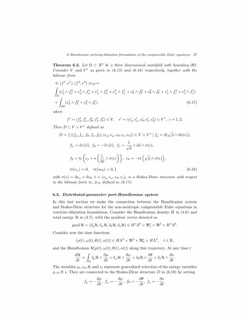
Theorem 6.2. Let Ω ⊂ R3 be a three dimensional manifold with boundary ∂Ω.

Consider V and V ⋆ as given in (6.15) and (6.16) respectively, together with the

bilinear form

≪ (f1, e1), (f2, e2)≫D:=∫

Ω

(e1ρ ∧ f2ρ + e2ρ ∧ f1

ρ + e1ω ∧ f2ω + e2ω ∧ f1

ω + e1θ ∧ f2θ + e2θ ∧ f1

θ + e1s ∧ f2s + e2s ∧ f1

s )

+

∫

∂Ω

(e1b ∧ f2b + e2b ∧ f1

b ) (6.17)

where

f i = (f iρ, f

iω, f

iθ, f

is, f

ib) ∈ V, ei = (eiρ, e

iω, e

iθ, e

is, e

ib) ∈ V ∗, i = 1, 2.

Then D ⊂ V × V ⋆ defined as

D = ((fρ, fω, fθ, fs, fb), (eρ, eω, eθ, es, eb)) ∈ V × V ⋆ | fρ = d(√

ρ ∧ dσ(e)),

fω = dγ(e), fθ = −δγ(e), fs =1√ρ∧ ds ∧ σ(e),

fb = tr

(

eρ + ⋆

(ζ

2ρ∧ σ(e)

))

, eb = −tr(√

ρ ∧ σ(e))

,

tr(eω) = 0, tr(⋆eθ) = 0, (6.18)

with σ(e) = deω + δeθ, e = (eρ, eω, eθ, es), is a Stokes-Dirac structure with respect

to the bilinear form ≪,≫D defined in (6.17).

6.3. Distributed-parameter port-Hamiltonian system

In this last section we make the connection between the Hamiltonian system

and Stokes-Dirac structure for the non-isentropic compressible Euler equations in

vorticity-dilatation formulation. Consider the Hamiltonian density H in (4.6) and

total energy H in (4.7), with the gradient vector denoted as

gradH = (δρH, δωH, δθH, δsH) ∈ H∗Λ0 ×B∗1 ×B3 ×H∗Λ0.

Consider now the time functions

(ρ(t), ω(t), θ(t), s(t)) ∈ HΛ3 ×B2 ×B∗0 ×HΛ3, t ∈ R,

and the Hamiltonian H[ρ(t), ω(t), θ(t), s(t)] along this trajectory. At any time t

dHdt

=

∫

Ω

δρH ∧∂ρ

∂t+ δωH ∧

∂ω

∂t+ δθH ∧

∂θ

∂t+ δsH ∧

∂s

∂t.

The variables ρt, ωt, θt and st represent generalized velocities of the energy variables

ρ, ω, θ, s. They are connected to the Stokes-Dirac structure D in (6.18) by setting

fρ = −∂ρ

∂t, fω = −∂ω

∂t, fθ = −∂θ

∂t, fs = −

∂s

∂t.


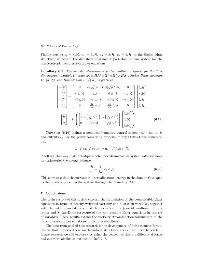
Finally, setting eρ = δρH, eω = δωH, eθ = δθH, es = δsH, in the Stokes-Dirac

structure, we obtain the distributed-parameter port-Hamiltonian system for the

non-isentropic compressible Euler equations.

Corollary 6.1. The distributed-parameter port-Hamiltonian system for the three

dimensional manifold Ω, state space HΛ3×B2×B∗0×HΛ3, Stokes-Dirac structure

D, (6.18), and Hamiltonian H, (4.6), is given as

−∂ρ∂t

−∂ω∂t

−∂θ∂t

−∂s∂t

=

0 d(√ρ ∧ d·) d(

√ρ ∧ δ·) 0

dγρ(·) dγω(·) dγθ(·) dγs(·)−δγρ(·) −δγω(·) −δγθ(·) −δγs(·)

0 ds√ρ∧ d· ds√

ρ∧ δ· 0

δρHδωHδθHδsH

[fb

eb

]

= tr

1 ⋆

(ζ2ρ ∧ d·

)

⋆(

ζ2ρ ∧ δ·

)

0 −√ρ ∧ d· −√ρ ∧ δ·

δρHδωHδθH

. (6.19)

Note that (6.19) defines a nonlinear boundary control system, with inputs fband outputs eb. By the power-conserving property of any Stokes-Dirac structure,

i.e.,

≪ (f, e), (f, e)≫D= 0, ∀(f, e) ∈ D,

it follows that any distributed-parameter port-Hamiltonian system satisfies along

its trajectories the energy balance

dHdt

=

∫

∂Ω

eb ∧ fb. (6.20)

This expresses that the increase in internally stored energy in the domain Ω is equal

to the power supplied to the system through the boundary ∂Ω.

7. Conclusions

The main results of this article concern the formulation of the compressible Euler

equations in terms of density weighted vorticity and dilatation variables, together

with the entropy and density, and the derivation of a (port)-Hamiltonian formu-

lation and Stokes-Dirac structure of the compressible Euler equations in this set

of variables. These results extend the vorticity-streamfunction formulation of the

incompressible Euler equations to compressible flows.

The long term goal of this research is the development of finite element formu-

lations that preserve these mathematical structures also at the discrete level. In

future research we will explore this using the concept of discrete differential forms

and exterior calculus as outlined in Ref. 2, 3.


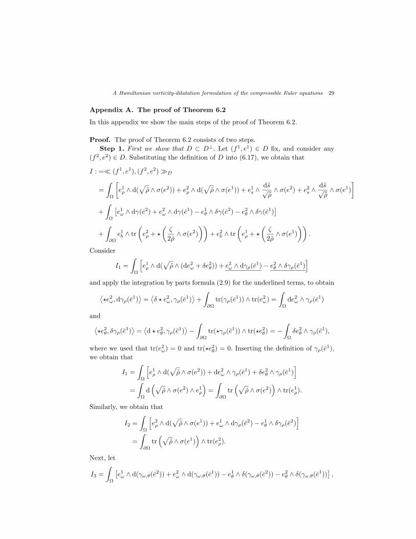
Appendix A. The proof of Theorem 6.2

In this appendix we show the main steps of the proof of Theorem 6.2.

Proof. The proof of Theorem 6.2 consists of two steps.

Step 1. First we show that D ⊂ D⊥. Let (f1, e1) ∈ D fix, and consider any

(f2, e2) ∈ D. Substituting the definition of D into (6.17), we obtain that

I : =≪ (f1, e1), (f2, e2)≫D

=

∫

Ω

[

e1ρ ∧ d(√

ρ ∧ σ(e2)) + e2ρ ∧ d(√

ρ ∧ σ(e1)) + e1s ∧ds√ρ∧ σ(e2) + e2s ∧

ds√ρ∧ σ(e1)

]

+

∫

Ω

[e1ω ∧ dγ(e2) + e2ω ∧ dγ(e1)− e1θ ∧ δγ(e2)− e2θ ∧ δγ(e1)

]

+

∫

∂Ω

e1b ∧ tr

(

e2ρ + ⋆

(ζ

2ρ∧ σ(e2)

))

+ e2b ∧ tr

(

e1ρ + ⋆

(ζ

2ρ∧ σ(e1)

))

.

Consider

I1 =

∫

Ω

[

e1ρ ∧ d(√

ρ ∧ (de2ω + δe2θ)) + e2ω ∧ dγρ(e1)− e2θ ∧ δγρ(e

1)]

and apply the integration by parts formula (2.9) for the underlined terms, to obtain

⟨⋆e2ω, dγρ(e

1)⟩=

⟨δ ⋆ e2ω, γρ(e

1)⟩+

∫

∂Ω

tr(γρ(e1)) ∧ tr(e2ω) =

∫

Ω

de2ω ∧ γρ(e1)

and

⟨⋆e2θ, δγρ(e

1)⟩=

⟨d ⋆ e2θ, γρ(e

1)⟩−

∫

∂Ω

tr(⋆γρ(e1)) ∧ tr(⋆e2θ) = −

∫

Ω

δe2θ ∧ γρ(e1),

where we used that tr(e2ω) = 0 and tr(⋆e2θ) = 0. Inserting the definition of γρ(e1),

we obtain that

I1 =

∫

Ω

[

e1ρ ∧ d(√

ρ ∧ σ(e2)) + de2ω ∧ γρ(e1) + δe2θ ∧ γρ(e

1)]

=

∫

Ω

d(√

ρ ∧ σ(e2) ∧ e1ρ

)

=

∫

∂Ω

tr(√

ρ ∧ σ(e2))

∧ tr(e1ρ).

Similarly, we obtain that

I2 =

∫

Ω

[

e2ρ ∧ d(√

ρ ∧ σ(e1)) + e1ω ∧ dγρ(e2)− e1θ ∧ δγρ(e

2)]

=

∫

∂Ω

tr(√

ρ ∧ σ(e1))

∧ tr(e2ρ).

Next, let

I3 =

∫

Ω

[e1ω ∧ d(γω,θ(e

2)) + e2ω ∧ d(γω,θ(e1))− e1θ ∧ δ(γω,θ(e

2))− e2θ ∧ δ(γω,θ(e1))

],


with γω,θ(·) defined in (6.14). Note that when applied to ei, α(F) is replaced by

σ(ei). Apply again partial integration and use that tr(eiω) = 0 and tr(⋆eiθ) = 0 to

obtain

I3 =

∫

Ω

[de1ω ∧ γω,θ(e

2) + de2ω ∧ γω,θ(e1) + δe1θ ∧ γω,θ(e

2) + δe2θ ∧ γω,θ(e1)]

=

∫

Ω

[σ(e1) ∧ γω,θ(e

2) + σ(e2) ∧ γω,θ(e1)].

Inserting the definition of γω,θ(ei), i = 1, 2 and applying again partial integration,

the above integral will reduce to

I3 =

∫

∂Ω

tr(√

ρ∧σ(e2))∧tr(

⋆(σ(e1) ∧ ζ

2ρ)

)

+tr(√

ρ∧σ(e1))∧tr(

⋆(σ(e2) ∧ ζ

2ρ)

)

.

Finally, observe that the term containing the entropy

I4 =

∫

Ω

[

e1s ∧ds√ρ∧ σ(e2) + e2s ∧

ds√ρ∧ σ(e1) + σ(e2) ∧ γs(e

1) + σ(e1) ∧ γs(e2)

]

,

is zero when we insert γs(ei) = − ds√

ρ∧ eis, i = 1, 2. Combining all terms, we obtain

that

I =

∫

∂Ω

tr

(

e1ρ + ⋆

(

σ(e1) ∧ ζ

2ρ

))

∧(

tr(√

ρ ∧ σ(e2)) + e2b

)

+ tr

(

e2ρ + ⋆

(

σ(e2) ∧ ζ

2ρ

))

∧(

tr(√

ρ ∧ σ(e1)) + e1b

)

= 0,

where the last equality is true since in D we have eib = − tr(√ρ ∧ σ(ei)), i = 1, 2.

Hence, we proved that the bilinear form (6.17) is zero for all (f2, e2) ∈ D. Therefore,

(f2, e2) ∈ D⊥.

Step 2. Next we show that D⊥ ⊂ D. Let (f1, e1) ∈ D⊥. Then,

J :=≪ (f1, e1), (f2, e2)≫D = 0, ∀(f2, e2) ∈ D. (A.1)

Since (f2, e2) ∈ D, the inner product above is

J =

∫

Ω

[

e1ρ ∧ d(√

ρ ∧ σ(e2)) + e2ρ ∧ f2ρ + e1ω ∧ d ⋆ γ(e2) + e2ω ∧ f1

ω

+e1θ ∧ ⋆dγ(e2) + e2θ ∧ f1θ + e1s ∧

1√ρ∧ ds ∧ σ(e2) + e2s ∧ f1

s

]

+

∫

∂Ω

[

e1b ∧ tr

(

e2ρ + ⋆

(

σ(e2) ∧ ζ

2ρ

))

− tr(√

ρ ∧ σ(e2)) ∧ f1b

]

Take e2ρ ∈ Λ0(Ω), e2ω ∈ Λ1(Ω), e2θ ∈ Λ3(Ω), such that tr(e2ρ) = 0,

tr(

⋆(

σ(e2) ∧ ζ2ρ

))

= 0 and tr(√ρ ∧ σ(e2)) = 0. Then the boundary integral in

J vanishes. After partial integration and using these vanishing traces, we obtain


that f1ρ , f

1ω, f

1θ are defined as in the Stokes-Dirac structure (6.18). The remaining

part of the proof is completely analogous to Step 2 in the proof of Theorem 6.1.

Acknowledgment

The research of M. Polner was partially supported by the Hungarian Scientific

Research Fund, Grant No. K75517 and by the TAMOP-4.2.2/08/1/2008-0008 pro-

gram of the Hungarian National Development Agency. The research of J.J.W. van

der Vegt was partially supported by the High-end Foreign Experts Recruitment

Program (GDW20137100168), while the author was in residence at the University

of Science and Technology of China in Hefei, China.

References

1. V.I. Arnold and B.A. Khesin, Topological methods in Hydrodynamics, Springer 1999.2. D.N. Arnold, R.S. Falk and R. Winther, Finite element exterior calculus, homological

techniques, and applications, Acta Numer., 15 (2006) 1–155.3. D. N. Arnold, R. S. Falk and R. Winther, Finite element exterior calculus: from Hodge

theory to numerical stability, Bull. Amer. Math. Soc., 47 (2010), no. 2, 281–354.4. S. Brenner and R. Scott, Mathematical theory of finite element methods, Texts in

Applied Mathematics, Springer-Verlag, New York, 1994. MR 95f:650015. J. Bruning and M. Lesch, Hilbert complexes, J. Funct. Anal. 108 (1992), no. 1, 88–132.6. G.-H. Cottet and P.D. Koumoutsakos, Vortex methods. Theory and practice, Cam-

bridge University Press, 2000.7. P.W. Gross, P.R. Kotiuga, Electromagnetic theory and computation: A topological

approach, Cambridge University Press, MSRI monograph, 2004.8. M. Feistauer, J. Felcman, I. Straskraba, Mathematical and computational methods for

compressible flow, Clarendon Press, Oxford, 2003.9. J.E. Marsden, T.S. Ratiu, Introduction to mechanics and symmetry, Texts in Applied

Mathematics, 17, Springer-Verlag, New York, 1994.10. P.J. Morrison, Hamiltonian description of the ideal fluid, Rev. Mod. Phys., 70 (1998)

467–521.11. P.J. Morrison and J.M. Green, Noncanonical Hamiltonian Density Formulation of

Hydrodynamics and Ideal Magnetohydrodynamics, Phys. Rev. Lett., 45 (1980) 790–794.

12. A. Novotny and I. Straskraba, Introduction to the mathematical theory of compressible

flow, Oxford University Press, 2004.13. A.J. van der Schaft, B.M. Maschke, Fluid dynamical systems as Hamiltonian boundary

control systems, Proc. 40th IEEE Conf. on Decision and Control, Orlando, Florida(2001) 4497–4502.

14. A.J. van der Schaft, B.M. Maschke, Hamiltonian formulation of distributed-parametersystems with boundary energy flow, Journal of Geometry and Physics, 42 (2002) 166–194.

15. G. Schwarz, Hodge decomposition: A method for solving boundary value problems,

Lecture Notes in Mathematics, 1607, Springer-Verlag, 1995.

Documents

A HAMILTONIAN VORTICITY-DILATATION FORMULATION OF … · vorticity and dilatation, and to formulate the Euler equations in terms of these new variables. Section 4 deals with the Hamiltonian