Embed Size (px)
Citation preview
A hands-on lesson on classical spectroscopicmethods
Maria Tsantaki
Osservatorio Astrofisico di Arcetri-INAF
22 September 2021
Stellar spectroscopy and Astrophysical parametrisation from Gaia to LargeSpectroscopic surveys, 21-23 September 2021
1 / 52
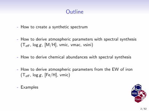
Outline
- How to create a synthetic spectrum
- How to derive atmospheric parameters with spectral synthesis(Teff , log g , [M/H], vmic, vmac, vsini)
- How to derive chemical abundances with spectral synthesis
- How to derive atmospheric parameters from the EW of iron(Teff , log g , [Fe/H], vmic)
- Examples
2 / 52
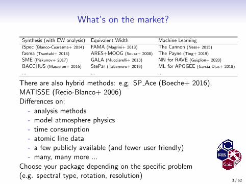
What’s on the market?
Synthesis (with EW analysis) Equivalent Width Machine Learning
iSpec (Blanco-Cuaresma+ 2014) FAMA (Magrini+ 2013) The Cannon (Ness+ 2015)
fasma (Tsantaki+ 2018) ARES+MOOG (Sousa+ 2008) The Payne (Ting+ 2019)
SME (Piskunov+ 2017) GALA (Mucciarelli+ 2013) NN for RAVE (Guiglion+ 2020)
BACCHUS (Masseron+ 2016) StePar (Tabernero+ 2019) ML for APOGEE (Garcia-Dias+ 2018)
... ... ...
There are also hybrid methods: e.g. SP Ace (Boeche+ 2016),MATISSE (Recio-Blanco+ 2006)Differences on:
- analysis methods- model atmosphere physics- time consumption- atomic line data- a few publicly available (and fewer user friendly)- many, many more ...
Choose your package depending on the specific problem(e.g. spectral type, rotation, resolution)
3 / 52
1. How to create a synthetic spectrum
4 / 52
1. How to get the flux at the top of the photosphere
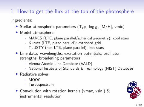
Ingredients:
• Stellar atmospheric parameters (Teff , log g , [M/H], vmic)• Model atmosphere
- MARCS (LTE, plane parallel/spherical geometry): cool stars- Kurucz (LTE, plane parallel): extended grid- TLUSTY (non-LTE, plane parallel): hot stars
• Line data: wavelengths, excitation potentials, oscillatorstrengths, broadening parameters
- Vienna Atomic Line Database (VALD)- National Institute of Standards & Technology (NIST) Database
• Radiative solver
- MOOG- Turbospectrum
• Convolution with rotation kernels (vmac, vsini) &instrumental resolution
5 / 52
1. How to get the flux at the top of the photosphere
Ingredients:
• Stellar atmospheric parameters (Teff , log g , [M/H], vmic)• Model atmosphere
- MARCS (LTE, plane parallel/spherical geometry): cool stars- Kurucz (LTE, plane parallel): extended grid- TLUSTY (non-LTE, plane parallel): hot stars
• Line data: wavelengths, excitation potentials, oscillatorstrengths, broadening parameters
- Vienna Atomic Line Database (VALD)- National Institute of Standards & Technology (NIST) Database
• Radiative solver
- MOOG- Turbospectrum
• Convolution with rotation kernels (vmac, vsini) &instrumental resolution
6 / 52
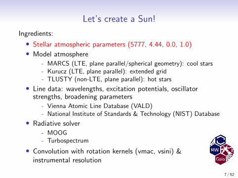
Let’s create a Sun!
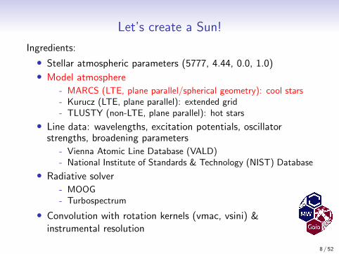
Ingredients:
• Stellar atmospheric parameters (5777, 4.44, 0.0, 1.0)• Model atmosphere
- MARCS (LTE, plane parallel/spherical geometry): cool stars- Kurucz (LTE, plane parallel): extended grid- TLUSTY (non-LTE, plane parallel): hot stars
• Line data: wavelengths, excitation potentials, oscillatorstrengths, broadening parameters
- Vienna Atomic Line Database (VALD)- National Institute of Standards & Technology (NIST) Database
• Radiative solver
- MOOG- Turbospectrum
• Convolution with rotation kernels (vmac, vsini) &instrumental resolution
7 / 52
Let’s create a Sun!
Ingredients:
• Stellar atmospheric parameters (5777, 4.44, 0.0, 1.0)• Model atmosphere
- MARCS (LTE, plane parallel/spherical geometry): cool stars- Kurucz (LTE, plane parallel): extended grid- TLUSTY (non-LTE, plane parallel): hot stars
• Line data: wavelengths, excitation potentials, oscillatorstrengths, broadening parameters
- Vienna Atomic Line Database (VALD)- National Institute of Standards & Technology (NIST) Database
• Radiative solver
- MOOG- Turbospectrum
• Convolution with rotation kernels (vmac, vsini) &instrumental resolution
8 / 52
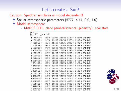
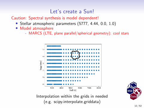
Let’s create a Sun!Caution: Spectral synthesis is model dependent!• Stellar atmospheric parameters (5777, 4.44, 0.0, 1.0)• Model atmosphere
- MARCS (LTE, plane parallel/spherical geometry): cool stars
Interpolation within the grids in needed.
9 / 52
Let’s create a Sun!Caution: Spectral synthesis is model dependent!• Stellar atmospheric parameters (5777, 4.44, 0.0, 1.0)• Model atmosphere
- MARCS (LTE, plane parallel/spherical geometry): cool stars
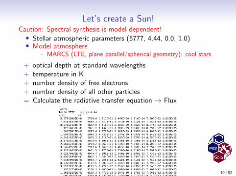
+ optical depth at standard wavelengths+ temperature in K+ number density of free electrons+ number density of all other particles= Calculate the radiative transfer equation → Flux
10 / 52
Let’s create a Sun!Caution: Spectral synthesis is model dependent!• Stellar atmospheric parameters (5777, 4.44, 0.0, 1.0)• Model atmosphere
- MARCS (LTE, plane parallel/spherical geometry): cool stars
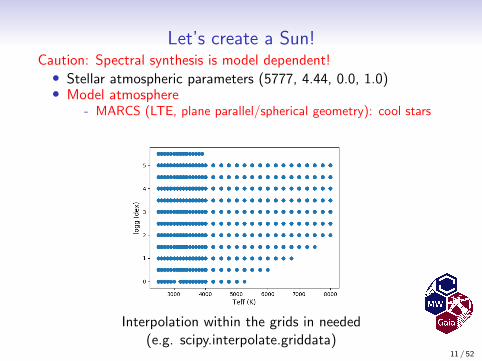
Interpolation within the grids in needed(e.g. scipy.interpolate.griddata)
11 / 52
Let’s create a Sun!Caution: Spectral synthesis is model dependent!• Stellar atmospheric parameters (5777, 4.44, 0.0, 1.0)• Model atmosphere
- MARCS (LTE, plane parallel/spherical geometry): cool stars
Interpolation within the grids in needed(e.g. scipy.interpolate.griddata)
12 / 52
Let’s create a Sun!
Ingredients:
• Stellar atmospheric parameters (5777, 4.44, 0.0, 1.0)• Model atmosphere
- MARCS (LTE, plane parallel/spherical geometry): cool stars- Kurucz (LTE, plane parallel): extended grid- TLUSTY (non-LTE, plane parallel): hot stars
• Line data: wavelengths, excitation potentials, oscillatorstrengths, broadening parameters
- Vienna Atomic Line Database (VALD)- National Institute of Standards & Technology (NIST) Database
• Radiative solver
- MOOG- Turbospectrum
• Convolution with rotation kernels (vmac, vsini) &instrumental resolution
13 / 52
Let’s create a Sun!Ingredients:• Stellar atmospheric parameters (5777, 4.44, 0.0, 1.0)• Model atmosphere
- MARCS (LTE, plane parallel/spherical geometry): cool stars- Kurucz (LTE, plane parallel): extended grid- TLUSTY (non-LTE, plane parallel): hot stars
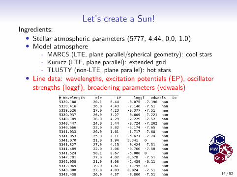
• Line data: wavelengths, excitation potentials (EP), oscillatorstrengths (loggf), broadening parameters (vdwaals)
14 / 52
Let’s create a Sun!Ingredients:• Stellar atmospheric parameters (5777, 4.44, 0.0, 1.0)• Model atmosphere
- MARCS (LTE, plane parallel/spherical geometry): cool stars- Kurucz (LTE, plane parallel): extended grid- TLUSTY (non-LTE, plane parallel): hot stars
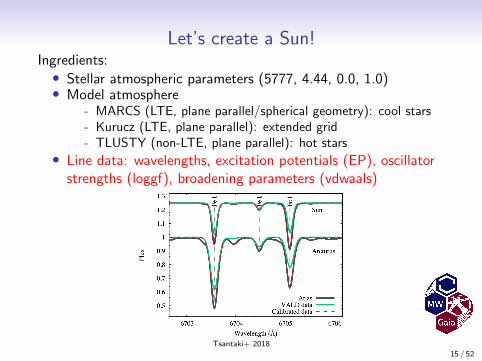
• Line data: wavelengths, excitation potentials (EP), oscillatorstrengths (loggf), broadening parameters (vdwaals)
Tsantaki+ 2018
15 / 52
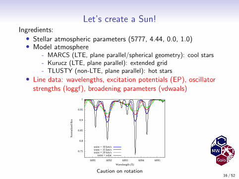
Let’s create a Sun!Ingredients:• Stellar atmospheric parameters (5777, 4.44, 0.0, 1.0)• Model atmosphere
- MARCS (LTE, plane parallel/spherical geometry): cool stars- Kurucz (LTE, plane parallel): extended grid- TLUSTY (non-LTE, plane parallel): hot stars
• Line data: wavelengths, excitation potentials (EP), oscillatorstrengths (loggf), broadening parameters (vdwaals)
0.75
0.8
0.85
0.9
0.95
1
6091 6092 6093 6094 6095
Nor
mal
ized
flux
Wavelength (Å)
υsini = 10 km/sυsini = 15 km/sυsini = 20 km/s
υsini = solar
Caution on rotation16 / 52
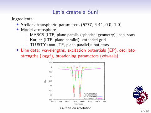
Let’s create a Sun!Ingredients:• Stellar atmospheric parameters (5777, 4.44, 0.0, 1.0)• Model atmosphere
- MARCS (LTE, plane parallel/spherical geometry): cool stars- Kurucz (LTE, plane parallel): extended grid- TLUSTY (non-LTE, plane parallel): hot stars
• Line data: wavelengths, excitation potentials (EP), oscillatorstrengths (loggf), broadening parameters (vdwaals)
0.65
0.7
0.75
0.8
0.85
0.9
0.95
1
1.05
6497.5 6498 6498.5 6499 6499.5 6500 6500.5 6501
Flu
x
Wavelength
Fe
I −−
Fe
I −−
R=110k (HARPS)R=48k (FEROS)
R=17k (GIRAFFE)R=2500 (VIMOS)
Caution on resolution17 / 52
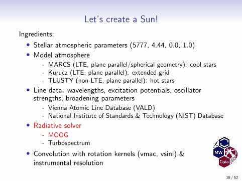
Let’s create a Sun!
Ingredients:
• Stellar atmospheric parameters (5777, 4.44, 0.0, 1.0)• Model atmosphere
- MARCS (LTE, plane parallel/spherical geometry): cool stars- Kurucz (LTE, plane parallel): extended grid- TLUSTY (non-LTE, plane parallel): hot stars
• Line data: wavelengths, excitation potentials, oscillatorstrengths, broadening parameters
- Vienna Atomic Line Database (VALD)- National Institute of Standards & Technology (NIST) Database
• Radiative solver
- MOOG- Turbospectrum
• Convolution with rotation kernels (vmac, vsini) &instrumental resolution
18 / 52
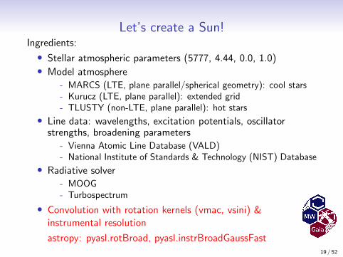
Let’s create a Sun!Ingredients:
• Stellar atmospheric parameters (5777, 4.44, 0.0, 1.0)• Model atmosphere
- MARCS (LTE, plane parallel/spherical geometry): cool stars- Kurucz (LTE, plane parallel): extended grid- TLUSTY (non-LTE, plane parallel): hot stars
• Line data: wavelengths, excitation potentials, oscillatorstrengths, broadening parameters
- Vienna Atomic Line Database (VALD)- National Institute of Standards & Technology (NIST) Database
• Radiative solver- MOOG- Turbospectrum
• Convolution with rotation kernels (vmac, vsini) &instrumental resolution
astropy: pyasl.rotBroad, pyasl.instrBroadGaussFast19 / 52
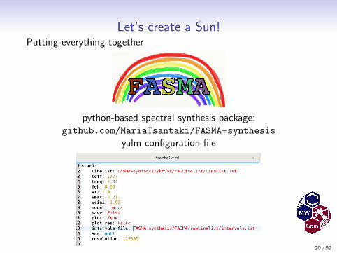
Let’s create a Sun!Putting everything together
python-based spectral synthesis package:github.com/MariaTsantaki/FASMA-synthesis
yalm configuration file
20 / 52

Questions?
21 / 52
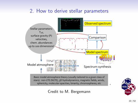
2. How to derive stellar parameters
[
lT[
�4
Modelspectrum
Observedspectrum
Comparison
Basicmodelatmospheretheory(usuallytailoredtoagivenclassofstars):non-LTE(NLTE),3Dhydrodynamics,magneticfields,winds,
sphericity,molecularopacities,binarity,chromospheres,etc
Stellarparameters:Teff,
surfacegravity(P)velocities,
chem.abundancesupto100dimensions!
SpectrumsynthesisModelatmosphere
Credit to M. Bergemann
22 / 52
2. How to derive stellar parameters
Pre-process the observed spectrum
• input format (fits, dat)
• cosmetic improvements
• wavelength re-sampling
• (local) normalization
Minimization process
• χ2 minimization (mpfit,Levenberg-Marquardt)
23 / 52

2. How to derive stellar parameters
Pre-process the observed spectrum
• input format (fits, dat)
• cosmetic improvements
• wavelength re-sampling
• (local) normalization
Minimization process
• χ2 minimization (mpfit,Levenberg-Marquardt)
24 / 52
2. How to derive stellar parameters
Pre-process the observed spectrum
• input format (fits, dat)
• cosmetic improvements
• wavelength re-sampling
• (local) normalization
Minimization process
• χ2 minimization (mpfit,Levenberg-Marquardt)
25 / 52

2. How to derive stellar parameters
Pre-process the observed spectrum
• input format (fits, dat)
• cosmetic improvements
• wavelength re-sampling
• (local) normalization
Minimization process
• χ2 minimization (mpfit,Levenberg-Marquardt)
26 / 52
2. How to derive stellar parameters
Pre-process the observed spectrum
• input format (fits, dat)
• cosmetic improvements
• wavelength re-sampling
• (local) normalization
Minimization process
• χ2 minimization (mpfit,Levenberg-Marquardt)
27 / 52
2. How to derive stellar parameters
Pre-process the observed spectrum
• input format (fits, dat)
• cosmetic improvements
• wavelength re-sampling
• (local) normalization
Minimization process
• χ2 minimization (mpfit,Levenberg-Marquardt)
28 / 52
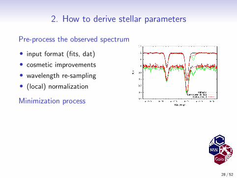
2. How to derive stellar parameters
Pre-process the observed spectrum
• input format (fits, dat)
• cosmetic improvements
• wavelength re-sampling
• (local) normalization
Minimization process
• χ2 minimization (mpfit,Levenberg-Marquardt)
29 / 52
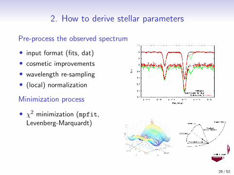
2. How to derive stellar parameters
Pre-process the observed spectrum
• input format (fits, dat)
• cosmetic improvements
• wavelength re-sampling
• (local) normalization
Minimization process
• χ2 minimization (mpfit,Levenberg-Marquardt)
• initial conditions
30 / 52
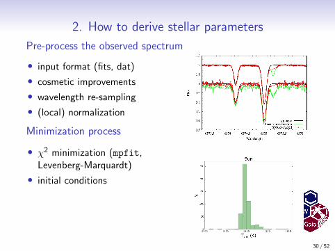
2. How to derive stellar parameters
Pre-process the observed spectrum
• input format (fits, dat)
• cosmetic improvements
• wavelength re-sampling
• (local) normalization
Minimization process
• χ2 minimization (mpfit,Levenberg-Marquardt)
• initial conditions
31 / 52
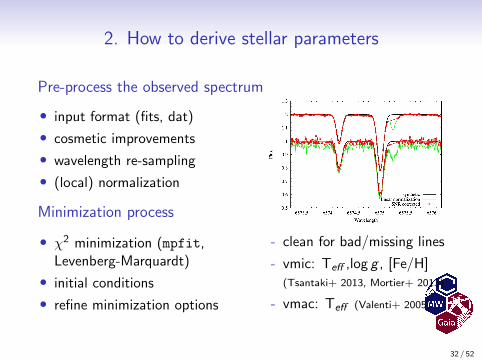
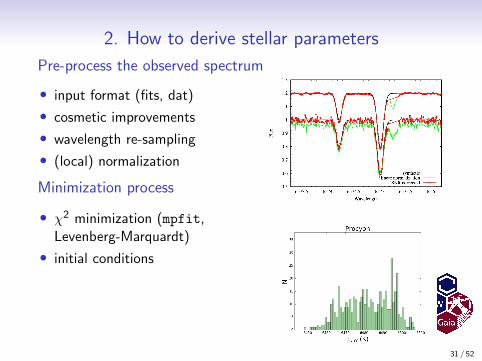
2. How to derive stellar parameters
Pre-process the observed spectrum
• input format (fits, dat)
• cosmetic improvements
• wavelength re-sampling
• (local) normalization
Minimization process
• χ2 minimization (mpfit,Levenberg-Marquardt)
• initial conditions
• refine minimization options
- clean for bad/missing lines
- vmic: Teff ,log g , [Fe/H](Tsantaki+ 2013, Mortier+ 2013)
- vmac: Teff (Valenti+ 2005)
32 / 52
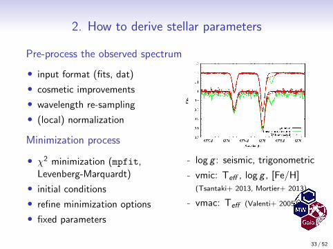
2. How to derive stellar parameters
Pre-process the observed spectrum
• input format (fits, dat)
• cosmetic improvements
• wavelength re-sampling
• (local) normalization
Minimization process
• χ2 minimization (mpfit,Levenberg-Marquardt)
• initial conditions
• refine minimization options
• fixed parameters
- log g : seismic, trigonometric
- vmic: Teff , log g , [Fe/H](Tsantaki+ 2013, Mortier+ 2013)
- vmac: Teff (Valenti+ 2005)
33 / 52
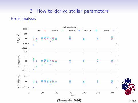
2. How to derive stellar parameters
Error analysis
High resolution
−100
−50
0
50
100
∆ T
eff
(K)
Sun Procyon Arcturus HD201891 del Eri
−0.2
−0.1
0
0.1
0.2
∆ l
og
g (
dex
)
−0.1
0
0.1
0 50 100 150 200 250 300
∆ [
M/H
] (d
ex)
S/N
(Tsantaki+ 2014) 34 / 52
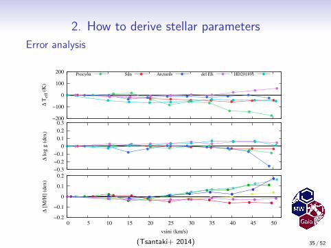
2. How to derive stellar parameters
Error analysis
−200
−100
0
100
200
∆ T
eff
(K)
Procyon Sun Arcturus del Eri HD201891
−0.3
−0.2
−0.1
0
0.1
0.2
0.3
∆ l
og
g (
dex
)
−0.2
−0.1
0
0.1
0.2
0 5 10 15 20 25 30 35 40 45 50
∆ [
M/H
] (d
ex)
vsini (km/s)
(Tsantaki+ 2014) 35 / 52
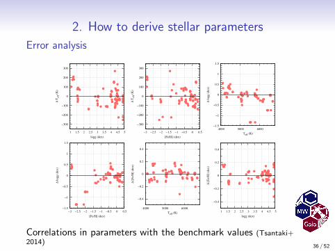
2. How to derive stellar parameters
Error analysis
−300
−200
−100
0
100
200
300
1 1.5 2 2.5 3 3.5 4 4.5 5
∆ T
eff
(K)
logg (dex)
−300
−200
−100
0
100
200
300
−3 −2.5 −2 −1.5 −1 −0.5 0 0.5∆
Tef
f (K
)
[Fe/H] (dex)
−1.5
−1
−0.5
0
0.5
1
1.5
4000 5000 6000
∆ l
ogg (
dex
)
Teff (K)
−1.5
−1
−0.5
0
0.5
1
1.5
−3 −2.5 −2 −1.5 −1 −0.5 0 0.5
∆ l
ogg (
dex
)
[Fe/H] (dex)
−0.4
−0.2
0
0.2
0.4
4000 5000 6000
∆ [
Fe/
H]
(dex
)
Teff (K)
−0.4
−0.2
0
0.2
0.4
1 1.5 2 2.5 3 3.5 4 4.5 5
∆ [
Fe/
H]
(dex
)
logg (dex)
Correlations in parameters with the benchmark values (Tsantaki+2014)
36 / 52
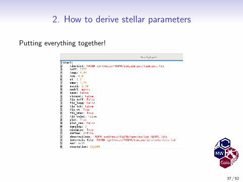
2. How to derive stellar parameters
Putting everything together!
37 / 52

Questions?
38 / 52
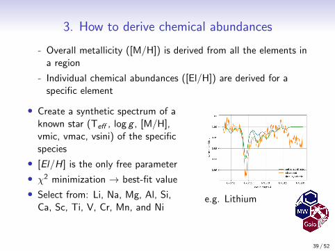
3. How to derive chemical abundances
- Overall metallicity ([M/H]) is derived from all the elements ina region
- Individual chemical abundances ([El/H]) are derived for aspecific element
• Create a synthetic spectrum of aknown star (Teff , log g , [M/H],vmic, vmac, vsini) of the specificspecies
• [El/H] is the only free parameter
• χ2 minimization → best-fit value
• Select from: Li, Na, Mg, Al, Si,Ca, Sc, Ti, V, Cr, Mn, and Ni
e.g. Lithium
39 / 52
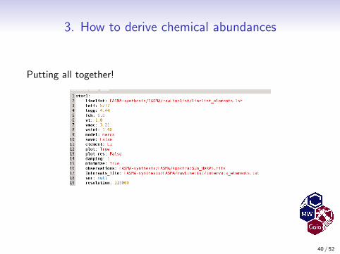
3. How to derive chemical abundances
Putting all together!
40 / 52
Questions?
41 / 52
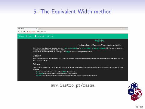
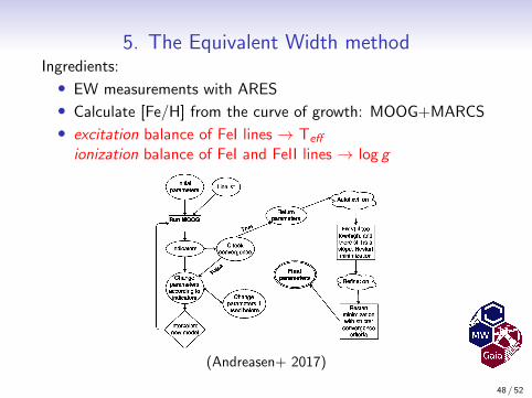
5. The Equivalent Width method
Ingredients:
• Line list of neutral (FeI) and ionized species (FeII)
• EW measurements (IRAF, daospec, ARES)
• Calculate [Fe/H] from the curve of growth
• Model atmospheres (MARCS, Kurucz)
• excitation balance of FeI lines → Teff
ionization balance of FeI and FeII lines → log g
42 / 52
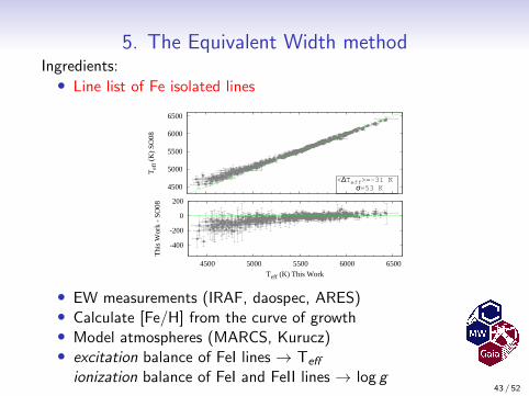
5. The Equivalent Width methodIngredients:• Line list of Fe isolated lines
-400
-200
0
200
4500 5000 5500 6000 6500
Thi
s W
ork
- SO
08
Teff (K) This Work
4500
5000
5500
6000
6500
Tef
f (K
) SO
08
<∆Teff
>=-31 K
σ=53 K
• EW measurements (IRAF, daospec, ARES)• Calculate [Fe/H] from the curve of growth• Model atmospheres (MARCS, Kurucz)• excitation balance of FeI lines → Teff
ionization balance of FeI and FeII lines → log g43 / 52
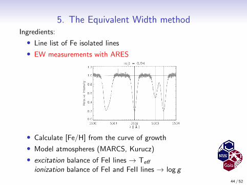
5. The Equivalent Width methodIngredients:
• Line list of Fe isolated lines
• EW measurements with ARES
• Calculate [Fe/H] from the curve of growth
• Model atmospheres (MARCS, Kurucz)
• excitation balance of FeI lines → Teff
ionization balance of FeI and FeII lines → log g
44 / 52
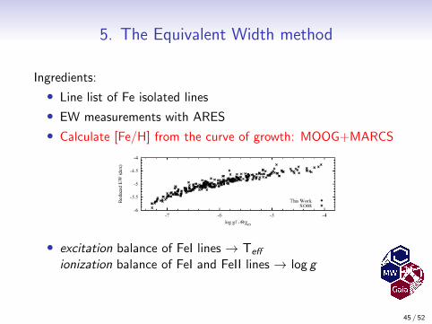
5. The Equivalent Width method
Ingredients:
• Line list of Fe isolated lines
• EW measurements with ARES
• Calculate [Fe/H] from the curve of growth: MOOG+MARCS
• excitation balance of FeI lines → Teff
ionization balance of FeI and FeII lines → log g
45 / 52
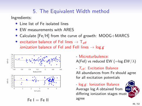
5. The Equivalent Width methodIngredients:
• Line list of Fe isolated lines
• EW measurements with ARES
• Calculate [Fe/H] from the curve of growth: MOOG+MARCS
• excitation balance of FeI lines → Teff
ionization balance of FeI and FeII lines → log g
7.1 7.2 7.3 7.4 7.5 7.6 7.7 7.8
0 1 2 3 4 5
A(F
e I)
E.P. (eV)
7.1 7.2 7.3 7.4 7.5 7.6 7.7 7.8
-5.8 -5.6 -5.4 -5.2 -5 -4.8 -4.6
A(F
e I)
Reduced EW
Fe I = Fe II
- Microturbulence:A(FeI) vs reduced EW (=log EW /λ)
- Teff : Excitation BalanceAll abundances from Fe should agreefor all excitation potentials
- log g : Ionization BalanceAverage logA obtained fromdiffering ionization stages mustagree
46 / 52
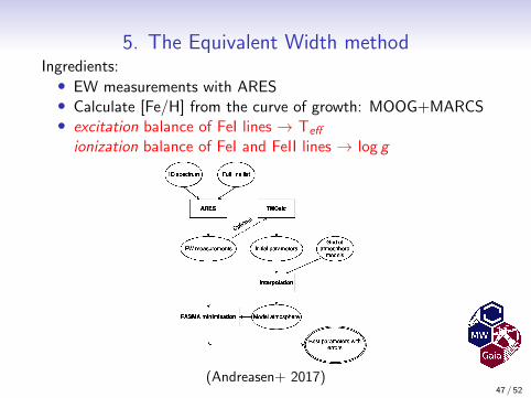
5. The Equivalent Width methodIngredients:• EW measurements with ARES• Calculate [Fe/H] from the curve of growth: MOOG+MARCS• excitation balance of FeI lines → Teff
ionization balance of FeI and FeII lines → log g
(Andreasen+ 2017)47 / 52
5. The Equivalent Width methodIngredients:
• EW measurements with ARES
• Calculate [Fe/H] from the curve of growth: MOOG+MARCS
• excitation balance of FeI lines → Teff
ionization balance of FeI and FeII lines → log g
(Andreasen+ 2017)
48 / 52
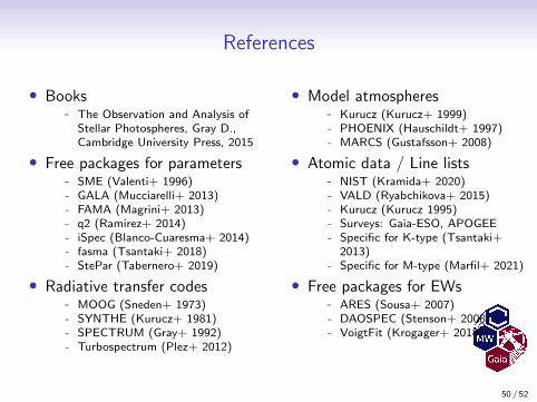
References
• Books- The Observation and Analysis of
Stellar Photospheres, Gray D.,Cambridge University Press, 2015
• Free packages for parameters- SME (Valenti+ 1996)- GALA (Mucciarelli+ 2013)- FAMA (Magrini+ 2013)- q2 (Ramirez+ 2014)- iSpec (Blanco-Cuaresma+ 2014)- fasma (Tsantaki+ 2018)- StePar (Tabernero+ 2019)
• Radiative transfer codes- MOOG (Sneden+ 1973)- SYNTHE (Kurucz+ 1981)- SPECTRUM (Gray+ 1992)- Turbospectrum (Plez+ 2012)
• Model atmospheres- Kurucz (Kurucz+ 1999)- PHOENIX (Hauschildt+ 1997)- MARCS (Gustafsson+ 2008)
• Atomic data / Line lists- NIST (Kramida+ 2020)- VALD (Ryabchikova+ 2015)- Kurucz (Kurucz 1995)- Surveys: Gaia-ESO, APOGEE- Specific for K-type (Tsantaki+
2013)- Specific for M-type (Marfil+ 2021)
• Free packages for EWs- ARES (Sousa+ 2007)- DAOSPEC (Stenson+ 2008)- VoigtFit (Krogager+ 2018)
50 / 52
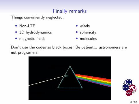
Finally remarksThings conviniently neglected:
• Non-LTE
• 3D hydrodynamics
• magnetic fields
• winds
• sphericity
• molecules
Don’t use the codes as black boxes. Be patient... astronomers arenot programers.
51 / 52
8. Exercise
Your turn!
52 / 52