A Heuristic Approach for Improvement Batch Plant …campusv.uaem.mx/cicos/imagenes/memorias/7mocicos2009/Articulos/… · A Heuristic Approach for Improvement Batch Plant Design under

A Heuristic Approach for Improvement Batch Plant Design under Imprecise Demand using Fuzzy Logics

Y. El-Hamzaouia ,J.A. Hernandeza , A.Bassamb

Centro de Investigación en Ingenieria y Ciencias Aplicadas (CIICAp), Universidad Autó-noma del Estado de Morelos (UAEM); Av. Universidad No. 1001, Col Chamilpa, C.P. 62209,

Cuernavaca, Morelos, Mexico b Centro de Investigación en Energía,Universidad Nacional Autónoma de México, Privada

Xochicalco s/n, Temixco, Mor. 62580, Mexico.

{youness, alfredo}@uaem.mx, [email protected]

Abstract. This paper deals with the problem of the improvement design of multiproduct batch chemical plants found in chemical engineering with imprecise demand. The objective of the batch plant design problem is to minimize the investment cost and find out the number and size of parallel equipment units in each stage. For this purpose, it is proposed to solve the problem in two differents ways: The first way is by using Monte Carlo Method (MC), the second way is by Genetic Algorithm (GA), that takes into account simultaneously, the imprecise demand using Fuzzy Logics with two criteria maximization of the Net Present Value (NPV) and Flexibility Index (FI). The results (number and size of equipment, investment cost, NPV, FI, Hi, CPU time) obtained by the GA are better than the MC. This methodology can help the decision makers and constitutes very a promising framework for finding a set of “good solutions”.

Key words: Genetic Algorithm, Monte Carlo, Fuzzy Logics, Batch Plant Design.

1. Introduction

In chemical engineering, precisely, in recent years, there has been an increased interest in the design of batch processes due to the growth of specialty chemical, food products, pharmaceutical and related industries aroused the current focus on the batch plant design problem (Cameron, 2008). Also the Process Engineering framework, batch processes are of growing industrial importance because of their flexibility and their ability to produce high added-value products in low volumes.

In economics, demand is the desire to own something and the ability to pay for it (Henning et al.1988). The term demand is also defined elsewhere as a measure of preferences that is weighted by income, but the market demand for such products is usually changeable, and at the stage of conceptual design of a batch plant, it is almost impossible to get the precise information on the future product demand over the lifetime of the plant. However, decisions must be made about the plant capacity. This capacity should be able to balance the product demand satisfaction (Henning et

M.A Cruz-Chávez, J.C Zavala Díaz(Eds):CICos2009, ISBN:978-607-00-1970-8, pp. 16 - 33, 2009.

al.1988). In the conventional optimal design of a multiproduct batch chemical plant (Hasebe et al.1979), a designer specifies the production requirements for each product and total production time for all products (Floudas et al.2005). The number required of volume and size of parallel equipment units in each stage is to be determined in order to minimize the investment cost.

Basically, batch plants are composed of items operating in a discontinuous way. Each batch then visits a fixed number of equipment items, as required by a given synthesis sequence (so-called production recipe) (Ponsich et al.2007).

For instance, the design of a multiproduct batch chemical plant is not only to minimize the investment cost, but also to minimize the operation cost, to minimize the total production time to maximize the revenue, and to maximize the flexibility index, simultaneously (Aguilar Lasserre et al, 2005).

On the other hand, the key point in the improvement design of batch plants under imprecision concerns the modeling of demand variations. The market demand for products resulting from the batch industry is usually changeable, and at the stage of conceptual design of a batch plant, it is almost impossible to obtain the precise information on the future product demand over the plant lifetime. Nevertheless, decisions must be made about on the plant capacity. This capacity should be able to balance the product demand satisfaction and extra-capacity in order to reduce the loss on the excessive investment cost or than on market share due to the varying product demands (Huang et al.2002).

The most recent common approaches treated in the dedicated literature represent the demand uncertainty with a probabilistic frame by means of Gaussian distributions. Yet, this assumption does not seem to be always a reliable representation of the reality, since in practice the parameters are interdependent and do not follow symmetric distribution rules, which leads to very complex conditional probabilities computations. An alternative treatment of the imprecision is constituted by using fuzzy concepts by Zadeh (1975). This approach, based on the arithmetic operations on fuzzy numbers, differs mainly from the probabilistic models insofar as distribution laws are not used. It considers the imprecise nature of the information, thus quantifying the imprecision by means of fuzzy sets that represent the ”more or less possible values”. In this study, we will only consider multiproduct batch plants, which mean that all the possible values”. Products follow the same operating steps (Bautista, 2007), the structure of the variables are the equipment sizes and number of each unit operation that generally takes discrete values. Based on Fuzzy concepts of the demand, the IBPD (Improvement Batch Plant Design) is solved by two techniques: Monte Carlo Method (MC) and Genetic Algorithm (GA). The aim of this work is to treat the improvement of multiproduct batch plant design under imprecise demand using MC and GA as tools of heuristic methods.

A Heuristic Approach for Improvement Batch Plant Design 17

The paper is organized as follows: Section 2 is devoted to the methodology and an overview of fuzzy set theory involved in the fuzzy framework, section 3 presents results and discussion. Finally the conclusions on this work are drawn.

2. Methodology

2.1 Process description

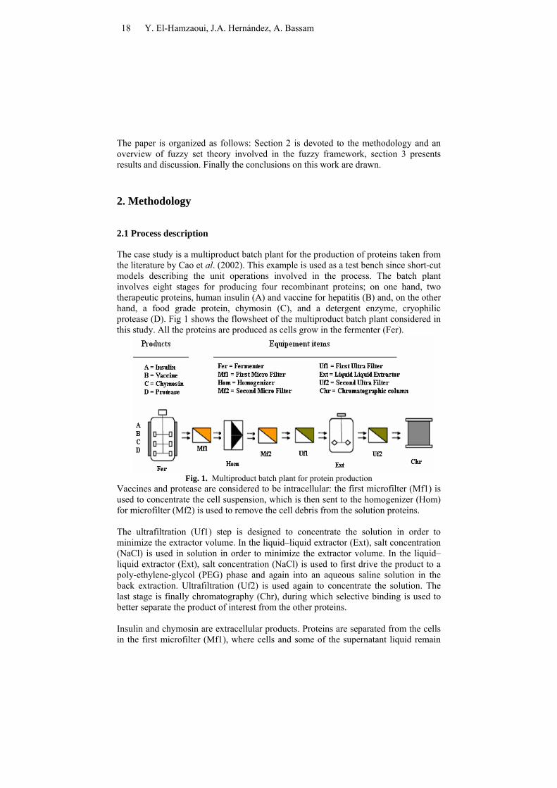
The case study is a multiproduct batch plant for the production of proteins taken from the literature by Cao et al. (2002). This example is used as a test bench since short-cut models describing the unit operations involved in the process. The batch plant involves eight stages for producing four recombinant proteins; on one hand, two therapeutic proteins, human insulin (A) and vaccine for hepatitis (B) and, on the other hand, a food grade protein, chymosin (C), and a detergent enzyme, cryophilic protease (D). Fig 1 shows the flowsheet of the multiproduct batch plant considered in this study. All the proteins are produced as cells grow in the fermenter (Fer).

Fig. 1. Multiproduct batch plant for protein production

Vaccines and protease are considered to be intracellular: the first microfilter (Mf1) is used to concentrate the cell suspension, which is then sent to the homogenizer (Hom) for microfilter (Mf2) is used to remove the cell debris from the solution proteins.

The ultrafiltration (Uf1) step is designed to concentrate the solution in order to minimize the extractor volume. In the liquid–liquid extractor (Ext), salt concentration (NaCl) is used in solution in order to minimize the extractor volume. In the liquid–liquid extractor (Ext), salt concentration (NaCl) is used to first drive the product to a poly-ethylene-glycol (PEG) phase and again into an aqueous saline solution in the back extraction. Ultrafiltration (Uf2) is used again to concentrate the solution. The last stage is finally chromatography (Chr), during which selective binding is used to better separate the product of interest from the other proteins.

Insulin and chymosin are extracellular products. Proteins are separated from the cells in the first microfilter (Mf1), where cells and some of the supernatant liquid remain

18 Y. El-Hamzaoui, J.A. Hernández, A. Bassam

behind. To reduce the amount of valuable products lost in the retentate, extra water is added to the cell suspension. The homogenizer (Hom) and microfilter (Mf2) for cell debris removal are not used when the product is extracellular. Nevertheless, the ultrafilter (Uf1) is necessary to concentrate the diluted solution prior to extraction. The final step of extraction (Ext), ultrafiltration (Uf2) and chromatography (Chr) are common to both the extracellular and intracellular products.

2.2. Fuzzy logics

The emergence of electronic commerce and business-to-business applications has, in a recent period, considerably changed the dynamics of the supplier–customer relationship. Indeed, customers can change more rapidly their orders to the suppliers and many enterprises have to organize their production even if the demand is not completely known at short term. On the other hand, the increasing need for integration and optimization in supply chains leads to a greater sensitivity to perturbations due to this uncertainty. These two elements clearly show the interest of taking into account as soon as possible the uncertainty on the demand and to propagate it along the production management mechanisms.

In the context of engineering design, an imprecise variable is a variable that may potentially assume any value within a possible range because the designer does not know a priori the final value that will emerge from the design process. The fuzzy set theory was introduced by Zadeh. (1975), to deal with problems in which a source of vagueness is involved. It is well recognized that fuzzy set theory offers a relevant framework to model imprecision.

In this section, only the key concepts from the theory of fuzzy sets that will be used for batch plant design are presented; more detail can be found in Kaufmann et al.(1988). Different forms can be used to model the membership functions of fuzzy numbers. We have chosen to use normalized trapezoidal fuzzy numbers (TrFNs) for modeling product demand, which can be represented by a membership function µ(X).

The proposed approach involves arithmetic operations on fuzzy numbers and quantifies the imprecision of the demand by means of trapezoidal fuzzy sets, as shown in Fig.2.We represent subjective judgments on future demand, given as linguistic values, such as “demand is around a certain value or interval [q2,q3] ” or “demand is not lower than a certain value”. For the design of the demand, we suppose that the products have a sure level of acceptance in market, represented by the interval [q2, q3]: This means that the demand has, in this interval, a certainty level α=1 that derives in TrFNs. On the other hand, the intervals [q1,q2] and [q3,q4] represent the demand “more or less possible values”. (See Fig. 2).


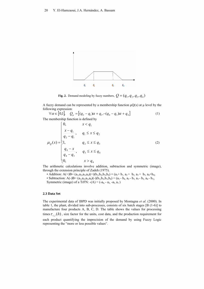
Fig. 2. Demand modeling by fuzzy numbers, ),,,( 4321 qqqqQ =

A fuzzy demand can be represented by a membership function µQ(x) at µ level by the following expression:

[ ] [ 434112 )(,)(,1,0 qqqqqqQ +−−+−=∈∀ ααα µ ] (1) The membership function is defined by

⎪⎪⎪⎪

⎩

⎪⎪⎪⎪

⎨

⎧

>

≤≤−−

≤≤

≤≤−−

<

=

4

4334

4

32

2112

1

1

,0

,

,1

,

,0

)(

qx

qxqqqxq

qxq

qxqqqqx

qx

xQµ (2)

The arithmetic calculations involve addition, subtraction and symmetric (image), through the extension principle of Zadeh (1975).

• Addition: A(+)B= (a1,a2,a3,a4)(+)(b1,b2,b3,b4) = (a1+ b1, a2 + b2, a3 + b3, a4+b4)• Subtraction: A(-)B= (a1,a2,a3,a4)(-)(b1,b2,b3,b4) = (a1 - b4, a2 - b3, a3 - b2, a4 - b1). Symmetric (image) of a TrFN: -(A) = (-a4, - a2, -a3, a1 )

2.3 Data Set

The experimental data of IBPD was initially proposed by Montagna et al. (2000). In table 1, the plant, divided into sub-processes, consists of six batch stages [B (1-6)] to manufacture four products A, B, C, D. The table shows the values for processing times )(, hjiτ , size factor for the units, cost data, and the production requirement for each product quantifying the imprecision of the demand by using Fuzzy Logic representing the “more or less possible values”.


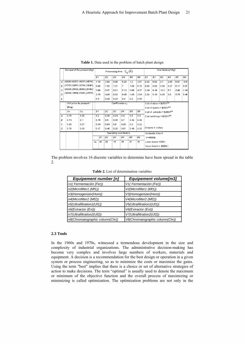
Table 1. Data used in the problem of batch plant design

The problem involves 16 discrete variables to determine have been spread in the table 2.

Table 2. List of determination variables

Equipement number [n] Equipement volume[m3]n1( Fermentación (Fer)) V1( Fermentación (Fer))n2(Microfilter1 (Mf1)) V2(Microfilter1 (Mf1))n3(Homogenizer(Hom)) V3(Homogenizer(Hom))n4(Microfilter2 (Mf2)) V4(Microfilter2 (Mf2))n5(Ultrafiltration1(Uf1)) V5(Ultrafiltration1(Uf1))

n8(Chromatographic column(Chr)) V8(Chromatographic column(Chr))

n6(Extractor (Ext)) V6(Extractor (Ext))n7(Ultrafiltration2(Uf2)) V7(Ultrafiltration2(Uf2))

2.3 Tools

In the 1960s and 1970s, witnessed a tremendous development in the size and complexity of industrial organizations. The administrative decision-making has become very complex and involves large numbers of workers, materials and equipment. A decision is a recommendation for the best design or operation in a given system or process engineering, so as to minimize the costs or maximize the gains. Using the term "best" implies that there is a choice or set of alternative strategies of action to make decisions. The term “optimal” is usually used to denote the maximum or minimum of the objective function and the overall process of maximizing or minimizing is called optimization. The optimization problems are not only in the


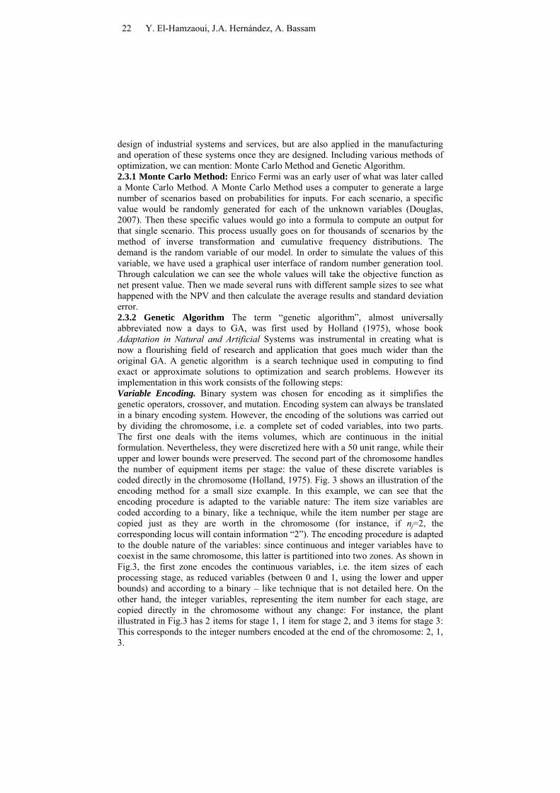
design of industrial systems and services, but are also applied in the manufacturing and operation of these systems once they are designed. Including various methods of optimization, we can mention: Monte Carlo Method and Genetic Algorithm. 2.3.1 Monte Carlo Method: Enrico Fermi was an early user of what was later called a Monte Carlo Method. A Monte Carlo Method uses a computer to generate a large number of scenarios based on probabilities for inputs. For each scenario, a specific value would be randomly generated for each of the unknown variables (Douglas, 2007). Then these specific values would go into a formula to compute an output for that single scenario. This process usually goes on for thousands of scenarios by the method of inverse transformation and cumulative frequency distributions. The demand is the random variable of our model. In order to simulate the values of this variable, we have used a graphical user interface of random number generation tool. Through calculation we can see the whole values will take the objective function as net present value. Then we made several runs with different sample sizes to see what happened with the NPV and then calculate the average results and standard deviation error. 2.3.2 Genetic Algorithm The term “genetic algorithm”, almost universally abbreviated now a days to GA, was first used by Holland (1975), whose book Adaptation in Natural and Artificial Systems was instrumental in creating what is now a flourishing field of research and application that goes much wider than the original GA. A genetic algorithm is a search technique used in computing to find exact or approximate solutions to optimization and search problems. However its implementation in this work consists of the following steps: Variable Encoding. Binary system was chosen for encoding as it simplifies the genetic operators, crossover, and mutation. Encoding system can always be translated in a binary encoding system. However, the encoding of the solutions was carried out by dividing the chromosome, i.e. a complete set of coded variables, into two parts. The first one deals with the items volumes, which are continuous in the initial formulation. Nevertheless, they were discretized here with a 50 unit range, while their upper and lower bounds were preserved. The second part of the chromosome handles the number of equipment items per stage: the value of these discrete variables is coded directly in the chromosome (Holland, 1975). Fig. 3 shows an illustration of the encoding method for a small size example. In this example, we can see that the encoding procedure is adapted to the variable nature: The item size variables are coded according to a binary, like a technique, while the item number per stage are copied just as they are worth in the chromosome (for instance, if nj=2, the corresponding locus will contain information “2”). The encoding procedure is adapted to the double nature of the variables: since continuous and integer variables have to coexist in the same chromosome, this latter is partitioned into two zones. As shown in Fig.3, the first zone encodes the continuous variables, i.e. the item sizes of each processing stage, as reduced variables (between 0 and 1, using the lower and upper bounds) and according to a binary – like technique that is not detailed here. On the other hand, the integer variables, representing the item number for each stage, are copied directly in the chromosome without any change: For instance, the plant illustrated in Fig.3 has 2 items for stage 1, 1 item for stage 2, and 3 items for stage 3: This corresponds to the integer numbers encoded at the end of the chromosome: 2, 1, 3.


Fig. 3. Illustration of the encoding method for a small size example

Creation of the initial population. The procedure of creating the initial population corresponds to random sampling of each decision variable within its specific range of variation. This strategy guarantees a population varied enough to explore large zones of the search space. Survival. For a given survival rate, the selection process is achieved via a classical biased roulette wheel. The selection is performed and each selected individual is included into the new population. Crossover Operation. To complete the new population, a classical one-point crossover is performed on pairs of individuals randomly chosen in the current population. Mutation Operation. After selection and crossover, mutation is then applied on the resulting population, with a fixed mutation rate. The number of individuals on which the mutation procedure is carried out is equal to the integer part of the value of the population size multiplied by the mutation rate. These individuals are chosen randomly among the population and then the procedure is applied. Elitism. The elitism consists in keeping the best individual from the current population to the next one.

2.4. Assumptions

The model formulation for IBPD’s problem adopted in this section is proposed by Karimi et al.(1989). It considers not only treatment in batch stages, which usually appears in all types of formulation, but also represents semi-continuous units that are part of the whole process (pumps, heat exchangers, etc). A semi-continuous unit is defined as a continuous unit alternating idle times and normal activity periods. Besides, this formulation takes into account mid-term intermediate storage tanks. They are just used to divide the whole process into sub-processes in order to store an amount of materials corresponding to the difference of each sub-process productivity.


This representation mode confers on the plant better flexibility for numerical resolution: It prevents the whole production process from being paralyzed by one limiting stage. So, a batch plant is finally represented as a series of batch stages (B), semi-continuous stages (SC) and storage tanks (T).The model is based on the following assumptions: (i) Devices used in the same production line can not be used again by the same product. (ii) Production is achieved through a series of single product campaigns. (iii) Units of the same batch or semi-continuous stage have the same type and size. (iv) All intermediate tank sizes are finite. (v) If a storage tank exists between two stages, the operation mode is “Finite Intermediate storage”. If not, the “Zero-Wait” policy is adopted. (vi) There is no limitation for utility. (vii) The cleaning time of the batch items is included in the processing time. (viii) The size of the items is continuous bounded variables.

2.5 Model Formulation

The model considers the synthesis of (I) products treated in (J) batch stages and (K) semi-continuous stages. Each batch stage consists of (mj) out-of-phase parallel items of the same size (Vj). Each semi-continuous stage consists of (nk) out-of-phase parallel items with the same processing rate (Rk) (i.e. treatment capacity, measured in volume unit per time unit). The item sizes (continuous variables) and equipment numbers per stage (discrete variables) are bounded. The (S-1) storage tanks, with size (Vs

*), divide the whole process into (S) sub-processes.

Following the above mentioned notation, IBPD’s problem can be formulated to minimize the investment cost for all items, maximizing the net present value and maximizing the flexibility index:

The investment cost (Cost), written as an exponential function of the unit size, is formulated in terms of the optimization variables, which represent the plant configuration:

∑∑∑===

++=S

s

sss

K

k

kkkk

J

j

jjjj VcRbnVamCostMin

111)()()()( γβα

(3)

Where aj and αj, bk and βk, Cs and γs are classical cost coefficients. A complete nomenclature is available in the Appendix. Eq. (3) shows that there is no fixed cost coefficient for any item. This may be unrealistic and will not tend towards minimization of the equipment number per stage. Nevertheless, this information was kept unchanged in order to compare our results with those found in the literature (Chunfeng et al.1996).


Instead of the investment cost recommended the economic criterion represents the NPV. This approach allows evaluating the impact of the plant over some years, taking into account the calculation of the net cash flow in terms of the present value of the money.

∑= +

++

+−−−+−−=

n

pnn

pppp

if

iAaADV

fCostNPVMax1 )1()1(

)1)(()( (4)

Eq.(4) underlines the fact that the objective function accounts not only for the investment cost, but also for the incomes from the sells (Vp), the operation costs (Dp) and depreciation (Ap) computed on n given time periods. Discount rates (r), taxes (a), and working capital (f) are also involved to update the money value. It is worth noting that since sales and operation costs depend on the uncertain demand parameter.

However, the Flexibility Index (FI) is formulated as the ratio between the new total production and initial demand:

∑

∑

=

=

+= I

ii

I

iii

Q

QQFIMax

1

1

* )()( (5)

This problem is subjected to three kinds of constraints:

(i) Variable bounding:

{ } maxmin,..,1 VVVjj j ≤≤∈∀ (6)

{ } maxmin,..,1 RRRkk k ≤≤∈∀ (7)

Volume of the items of each batch stage j and treatment capacity of each semi-continuous stage k. However, these variables are not continuous anymore and were discretized with an interval of 50 units between two possible values. This working mode was adopted in a view of realism. Indeed, since equipment manufacturers propose the items following defined size ranges, the design of operation unit equipments does not require a level of accuracy such as real number. Note however that the initial bounds on these size variables were kept unchanged, being for batch and semi-continuous, respectively: and , and .

jV kR

minV maxV minR maxR

Item number in batch stage j and item number in semi-continuous stage k.

These variables cannot exceed 3 items per stage (jm kn

3,1 ≤≥ kj nm ). (ii) Time constraint: the total production time for all products must be lower than a given time horizon H :


∑∑==

=≥I

i i

iI

ii od

QHH

11 Pr (8)

Where is the demand for product i. iQ(iii) Constraint on productivities: the global productivity for product i (of the whole process) is equal to the lowest local productivity (of each sub-process s).

{ } [ ]

Ssisi odlocMinodIi

∈=∈∀ PrPr,..1 (9)

These local productivities are calculated from the following equations: (a) Local productivities for product i in sub-process s:

{ } { } Lis

is

TBodlocisSsIi =∈∀∈∀ Pr,..,1,,..,1 (10)

(b) Limiting cycle time for product i in sub-process s: { } { } [ ]itij

Lis TMaxTSsIi Θ=∈∀∈∀ ,,..1,,..1 (11)

Where Js and Ks are, respectively, the sets of batch and semi-continuous stages in sub-process s. (c) Cycle time for product I in batch stage j:

{ } { }j

ijtitiij m

pTJjIi

+Θ+Θ=∈∀∈∀ + )1(,,..,1,,..,1 (12)

Where k and k+1 represent the semi-continuous stages before and after batch stage j. (d) Processing time of product i in batch stage j:

{ } { } { } dijisijijij BgppSsJjIi +=∈∀∈∀∈∀ 0,..,1,..,1,,..,1

(13) (e) Operating time for product i in semi-continuous stage : k

{ } { } { }kk

ikisik nR

DBSsKskIi =∈∀∈∀∈∀ θ,..,1,,..,1,,..,1 (14)

(f) Batch size of product i in sub-process : s

{ } { }⎥⎥⎦

⎤

⎢⎢⎣

⎡=∈∀∈∀

ij

jis S

VMinBSsIi ,..1,,..,1 (15)

(g) Finally, the size of intermediate storage tanks is estimated as the greatest size difference between the batches treated in two successive sub-processes:

{ } [ ])1()1((*Pr1,..,1 ++ Θ−Θ−+=−∈∀ tiLsi

Lisisis TTSodMaxVSs

(16)


3. Results and discussion

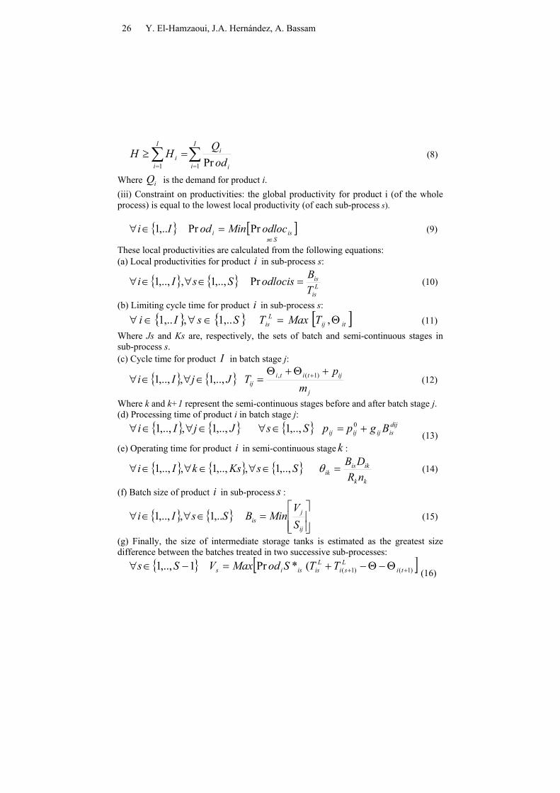
The results obtained by Monte Carlo Method, running the model 30 runs of 100000 iterations is given in Table 3, although Fig .5 shows equipment structure according to this result.

Table 3. Best design of batch plant by MC

V1 V2 V3 V4 V5 V6 V7 V810000.000 10000.000 10000.000 8692.625 9924.000 10000.000 899.877 6269.000

n1 n2 n3 n4 n5 n6 n7 n83 3 3 3 3 3 3 2

Volume [m3]

Equipment number [n]

%Std.Dev(FI)Cost

Max(NPV)%Std.Dev(NPV)

Max(FI)

1000000[$]15%

1.00000085

HiCPU time

15%1500000[$]

6000(h)20000*(s)

*CPU time was calculated for MC method on Microsoft Windows XP Professional Intel(R)D CPU 2.80 GHz., 2.99 GB of RAM.

Fig. 4. Equipment Structure according to the Table 3

However, the Genetic Algorithm parameters are displayed in Table 4.The reference values were taken from (Berard, 2000).

Table 4. Genetic algorithm parameters

Population size 200 Generation number 1000 Survival rate 0.50


Mutation rate 0.40 Elitism 1

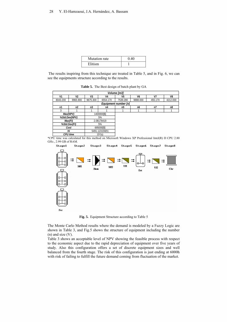
The results inspiring from this technique are treated in Table 5, and in Fig. 6, we can see the equipments structure according to the results.

Table 5. The Best design of batch plant by GA

V1 V2 V3 V4 V5 V6 V7 V88043.200 9965.900 9675.300 6554.170 7539.280 9888.000 455.170 4212.000

n1 n2 n3 n4 n5 n6 n7 n83 1 1 1 1 1 1 1

Hi 5491.123159(h)CPU time 15*(s)

%Std.Dev(FI) 5%Cost 695000[$]

%Std.Dev(NPV) 5%Max(FI) 2.08176419

Max(NPV) 1400000[$]

Volume [m3]

Equipment number [n]

*CPU time was calculated for this method on Microsoft Windows XP Professional Intel(R) D CPU 2.80 GHz., 2.99 GB of RAM.

Fig. 5. Equipment Structure according to Table 5

The Monte Carlo Method results where the demand is modeled by a Fuzzy Logic are shown in Table 3, and Fig.5 shows the structure of equipment including the number (n) and size (V). Table 3 shows an acceptable level of NPV showing the feasible process with respect to the economic aspect due to the rapid depreciation of equipment over five years of study. Also this configuration offers a set of discrete equipment sizes and well balanced from the fourth stage. The risk of this configuration is just ending at 6000h with risk of failing to fulfill the future demand coming from fluctuation of the market.


The typical results obtained by Genetic Algorithm after thirty runs guarantees the stochastic nature of the algorithm with demand modeled by a Fuzzy Logic, maximizing NPV and FI are shown in Table 5, and in Fig.6 had been indicated the structure of equipment. Also this configuration shows an excellent NPV with respect to the economical feasibility and indicates great flexibility in the process to fulfill future demand.

Table 5 shows a better NPV ($1,400,000) from the configuration obtained by GA optimization with respect to the MC. Also this process shows great flexibility (FI=2.08), taking into account, that the customers need the product each 6000h, the configuration created by Table 5 has 5491.12h as a total production time. This helps fulfill the increase future demand coming from fluctuation of the market. Also this configuration shows a very small Std. Dev (error): In addition, GA’s results are faster convergence (CPU=15s), and GA’s yield highly satisfactory could be touch to the global optimum.

However, the configuration showing by Monte Carlo Method (Table 3 and Fig.5 ) is expensive and the NPV obtained is very small, also The error is also high, and the time of the process calculation is slow(CPU=20000s~6h).

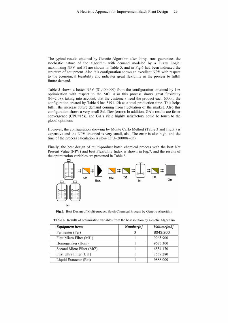
Finally, the best design of multi-product batch chemical process with the best Net Present Value (NPV) and best Flexibility Index is shown in Fig.7, and the results of the optimization variables are presented in Table 6.

Fig.6. Best Design of Multi-product Batch Chemical Process by Genetic Algorithm

Table 6. Results of optimization variables from the best solution by Genetic Algorithm

Equipment items Number[n] Volume[m3] Fermenter (Fer) 3 8043.200 First Micro Filter (Mf1) 1 9965.900 Homogenizer (Hom) 1 9675.300 Second Micro Filter (Mf2) 1 6554.170 First Ultra Filter (Uf1) 1 7539.280 Liquid Extractor (Ext) 1 9888.000


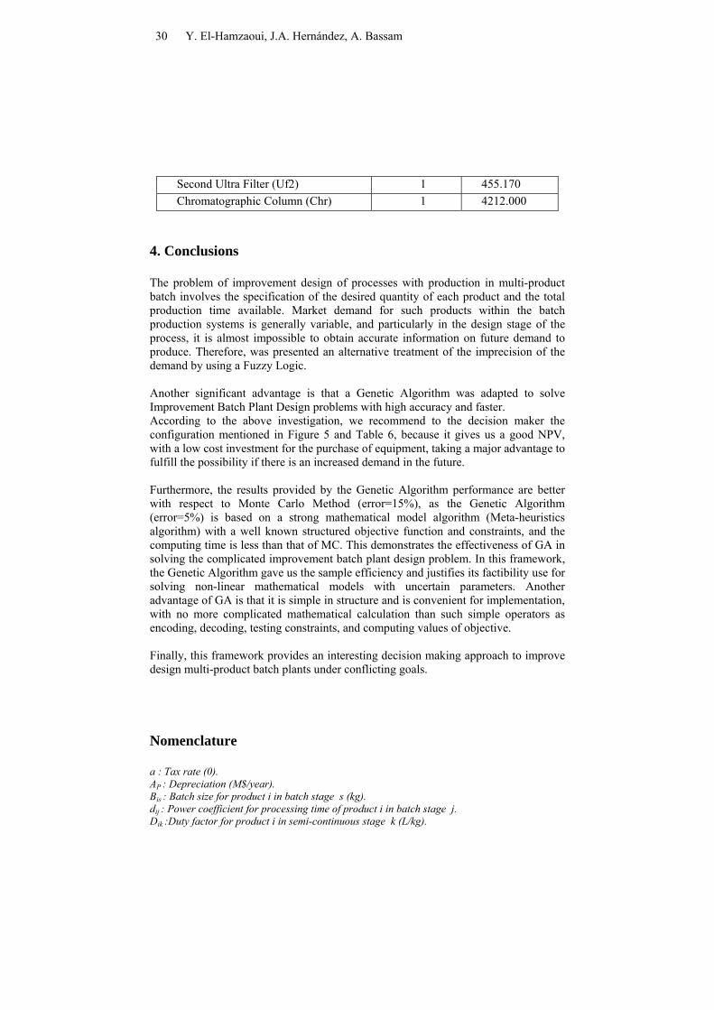
Second Ultra Filter (Uf2) 1 455.170 Chromatographic Column (Chr) 1 4212.000

4. Conclusions

The problem of improvement design of processes with production in multi-product batch involves the specification of the desired quantity of each product and the total production time available. Market demand for such products within the batch production systems is generally variable, and particularly in the design stage of the process, it is almost impossible to obtain accurate information on future demand to produce. Therefore, was presented an alternative treatment of the imprecision of the demand by using a Fuzzy Logic.

Another significant advantage is that a Genetic Algorithm was adapted to solve Improvement Batch Plant Design problems with high accuracy and faster. According to the above investigation, we recommend to the decision maker the configuration mentioned in Figure 5 and Table 6, because it gives us a good NPV, with a low cost investment for the purchase of equipment, taking a major advantage to fulfill the possibility if there is an increased demand in the future.

Furthermore, the results provided by the Genetic Algorithm performance are better with respect to Monte Carlo Method (error=15%), as the Genetic Algorithm (error=5%) is based on a strong mathematical model algorithm (Meta-heuristics algorithm) with a well known structured objective function and constraints, and the computing time is less than that of MC. This demonstrates the effectiveness of GA in solving the complicated improvement batch plant design problem. In this framework, the Genetic Algorithm gave us the sample efficiency and justifies its factibility use for solving non-linear mathematical models with uncertain parameters. Another advantage of GA is that it is simple in structure and is convenient for implementation, with no more complicated mathematical calculation than such simple operators as encoding, decoding, testing constraints, and computing values of objective.

Finally, this framework provides an interesting decision making approach to improve design multi-product batch plants under conflicting goals.

Nomenclature

a : Tax rate (0). AP : Depreciation (M$/year). Bis : Batch size for product i in batch stage s (kg). dij : Power coefficient for processing time of product i in batch stage j. Dik :Duty factor for product i in semi-continuous stage k (L/kg).


DP : Operation cost (M$/year). CP : Unit price of production cost ($/kg). Co : Unit price of operation cost ($/kg). CE : Operating cost factors. f : Working capital (M$). gij : Coefficient for processing time of product i in batch stage j. k : Index for semi-continuous stages. K : Total number of semi-continuous stages. Ks :Total number of semi-continuous stages in sub-process s. mj : Number of parallel out-of-phase items in batch stage j. M :Number of stages. n : Number of periods. nk : Number of parallel out-of-phase items in semi-continuous stage k. pij : Processing time of product i in batch stage j (h). pij

0 : Constant for calculation of processing time of product i in batch stage j( h). P : Number of products to be produced. prodi : Global productivity for product i (kg/h). prodlocis : Local productivity for product i in sub-process s (kg/h). Qi :Demand for product i. Rk : Processing rate for semi-continuous satge k (L/h). Rk

max : Maximum feasible processing rate for semi-continuous stage k (L/h). Rk

min : Minimum feasible processing rate for semi-continuous stage k (L/h). S : Total number of sub-processes. Sij : Size factor of product i in batch stage j (L/kg). Sis : Size factor of product i in intermediate storage tanks (L/kg). Tij : Cycling time of product i in batch stage j(h). Tis

L : Limiting cycling time of product i in sub-process s(h). Vj : Size of batch stage j (L). Vj

max : Maximum feasible size of batch stage j (L). Vj

min : Minimum feasible size of batch stage j (L). Vp : Revenue (M$/year). Vs : Size of intermediate storage tank (L). Greek letters

jα : Cost factor for batch stage j. kβ : Power cost coefficient for semi-continuous stage k.

sγ : Power cost coefficient for intermediate storage.

ikΘ : Operating time of product i in semi-continuous stage k.


References

1. Aguilar Lasserre, A. A, Azzaro-Pantel C, Pibouleau L, Domenech S. : Modelisation des imprecisions de la demande en conception optimale multicritère d’atelier discontinues.In: Proceedings of the SFGP (Sociètè Francias de Gènie de procedes), Toulouse, France (2005).

2. Bautista MA. Modelo y software para la interpretación de cantidades difusas en un

problema de diseño de procesos .MBA thesis, Instituto Tecnológico de Orizaba, México, 2007.

3. Berard, Stratègies de gestion de production dans un atelier flexible de chimie fine.

These de doctorate, INP ENSIGC Toulouse,France(2000).

4. Cameron, A Survey of industrial process modeling across the product and life cycle. Computers & Chemical Engineering Volume 32,Issue 3,24 March 2008, page420-438.

5. Cao DM, Yuan XG. Optimal design of batch plants with uncertain demands

considering switchover of operating modes of parallel units. Industrial Engineering and Chemistry Research 2002; 41(18):4616–25.

6. Chunfeng Wang, Hongying Quan,and Xien Xu ., Optimal Design of Multiproduct

Batch Chemical process Using Genetic Algorithm. Ind. Eng. Chem. Res. 1996, 35, 3560-3566.

7. Douglas Hubbard "How to Measure Anything: Finding the Value of Intangibles in

Business" p. 72, John Wiley & Sons, 2007

8. Floudas C.A., I.G. Akrotirianakis S, Caratzoulas, C.A. Meyer, J. Kallrath Global Optimization in the 21st century: Advances and challenges. Computers & Chemical Engineering volume 29, Issue 6, 15 May 2005, pages 1185.

9. Hasebe S.,Takeichiro Takamatsu, Iori Hashimoto Optimal scheduling and minimum

storage tank capacities in a process system with parallel batch units. Computers & Chemical Engineering volume 3, Issues 1-4,1979 pages 185-195).

10. Henning, N, Charles, and piogott William, and Scott, Robert Haney, Financial

Markets and the economy 5th ed, new Jersey, 1988.

11. Holland, J, Adaptation in Natural and Artificial Systems, 1975. Oxford University,Press

12. Huang HJ, Wang WF. Fuzzy decision-making design of chemical plant using mixed-

integer hybrid differential evolution. Computers and Chemical Engineering 2002; 26(12):1649–60.


13. Karimi IA Modi AK,. Design of multiproduct batch processes with finite

intermediate storage.Computers and Chemical Engineering 1989;13(1-2):127-39.

14. Kaufmann, A., Gupta, M. M. Fuzzy mathematical models in engineering and management s(1988). Science. North Holland.

15. Montagna, J. M., Vecchietti, A. R., Iribarren, O. A., Pinto, J. M., & Asenjom, J. A.

(2000). Optimal design of protein production plants with time and size factor process models. Biotechnology Progress, 16, 228–237.

16. Ponsich A, Azzaro-Pantel C, Domenech S, Pibouleau. Some Guidelines for Genetic

Algorithm Implemenetation in MINLP Batch Plant Design Problems, Ind. Eng. Chem. Res., 2007, 46 (3).

17. Zadeh LA. The concept of a linguistic variable and its application to approximate

reasoning.Information Sciences 1975;8(3):199–249.


Documents

A Heuristic Approach for Improvement Batch Plant …campusv.uaem.mx/cicos/imagenes/memorias/7mocicos2009/Articulos/… · A Heuristic Approach for Improvement Batch Plant Design under