NAVAL POSTGRADUATE SCHOOLMonterey, California

THESISA HEURISTIC SEARCH METHOD

OF SELECTING RANGE-RANGE SITESFOR HYDROGRAPHIC SURVEYS

by

Arnold F. Steed

September, 1991

Thesis Advisor:Co-Advisor:

Neil C. RoweEverett Carter

Approved for public release; distribution is unlimited

T258733

Unclassified

SECURITY CLASSIFICATION OF THIS PAGE

REPORT DOCUMENTATION PAGE

1a REPORT SECURITY CLASSIFICATION

UNCLASSIFIEDlb RESTRICTIVE MARKINGS

2a SECURITY CLASSIFICATION AUTHORITY

2b DECLASSIFICATION/DOWNGRADING SCHEDULE

3 DISTRIBUTION/AVAILABILITY OF REPORT

Approved for public release; distribution is unlimited.

4 PERFORMING ORGANIZATION REPORT NUMBER(S) 5 MONITORING ORGANIZATION REPORT NUMBER(S)

6a NAME OF PERFORMING ORGANIZATIONNaval Postgraduate School

6b OFFICE SYMBOL(If applicable)

35

7a NAME OF MONITORING ORGANIZATION

Naval Postgraduate School

6c ADDRESS (City, State, and ZIP Code)

Monterey, CA 93943-5000

7b ADDRESS (City, State, and ZIP Code)

Monterey, CA 93943-5000

8a NAME OF FUNDING/SPONSORING

ORGANIZATION8b OFFICE SYMBOL

(If applicable)

9 PROCUREMENT INSTRUMENT IDENTIFICATION NUMBER

8c ADDRESS (City, State, and ZIP Code) 10 SOURCE OF FUNDING NUMBERS

Proyrdm tlement No Project No Work unit Acceiiion

Number

1 1 TITLE (Include Security Classification)

A HEURISTIC SEARCH METHOD OF SELECTING RANGE-RANGE SITES FOR HYDROGRAPHIC SURVEYS

12 PERSONAL AUTHOR(S) Steed, Arnold F.

13a TYPE OF REPORT

Master's Thesis

13b TIME COVERED

From To

14 DATE OF REPORT (year, month, day)

September, 1991

15 PAGE COUNT123

16 SUPPLEMENTARY NOTATION

The views expressed in this thesis are those of the author and do not reflect the official policy or position of the Department of Defense or the U.S.

Government.

17 COSATI CODES

FIELD GROUP SUBGROUP

18 SUBJECT TERMS (continue on reverse if necessary and identify by block number)

Hydrography, navigation, heuristic search, artificial intelligence

19 ABSTRACT (continue on reverse if necessary and identify by block number)

One of the costliest aspects of many hydrographic surveys is establishing and occupying the navigation control stations. As budget cuts

force agencies to conduct their surveys more efficiently, minimizing the cost of these control networks will be of primary importance.

Because it has the ability to process numerical information faster than a human, a computer could be used to assist the survey planner in

selecting optimal shore sites, yet little work has actually been done in this area.

This thesis examines the possibility of using Artificial Intelligence (AI) to assist the survey planner in selecting navigation control

sites. A search program is presented which uses a number of heuristics to select sites and guide the search for an optimal solution. The

program was tested in several actual and idealized survey situations, and the results of these tests indicate that the heuristic search approach

has the potential of surpassing a human expert in the selection of an optimal set of sites.

20 DISTRIBUTION/AVAILABILITY OF ABSTRACT

Q UNCLASSIHtD/UNUMITED J SAME AS Ktl'ORl ] DTIC USERS

21 ABSTRACT SECURITY CLASSIFICATION

Unclassified

22a NAME OF RESPONSIBLE INDIVIDUAL

NeilC.Rowe22b TELEPHONE (Include Area code)

(408)646-2462

22c OFFICE SYMBOLCS/Rp

DD FORM 1473, 84 MAR 83 APR edition may be used until exhausted

All other editions are obsolete

SECURITY CLASSIFICATION OF THIS PAGE

Unclassified

Approved for public release; distribution is unlimited.

A Heuristic Search Method

of Selecting Range-Range Sites

for Hydrographic Surveys

by

Arnold F. .-Steed

Physical Scientist, Naval Oceanographic Office

B.S., University of Texas , 1987

Submitted in partial fulfillment

of the requirements for the degree of

MASTER OF SCIENCE IN HYDROGRAPHIC SCIENCE

from the

ABSTRACT

One of the costliest aspects of many hydrographic surveys is establishing and

occupying the navigation control stations. As budget cuts force agencies to conduct their

surveys more efficiently, minimizing the cost of these control networks will be of primary

importance. Because it has the ability to process numerical information faster than a

human, a computer could be used to assist the survey planner in selecting optimal shore

sites, yet little work has actually been done in this area.

This thesis examines the possibility of using Artificial Intelligence (AI) to assist the

survey planner in selecting navigation control sites. A search program is presented which

uses a number of heuristics to select sites and guide the search for an optimal solution.

The program was tested in several actual and idealized survey situations, and the results

of these tests indicate that the heuristic search approach has the potential of surpassing a

human expert in the selection of an optimal set of sites.

ui

6J

TABLE OF CONTENTS

I. INTRODUCTION 1

A. HYDROGRAPHIC SURVEY PLANNING 1

B. OPTIMIZING SITE LOCATIONS 2

C. OVERVIEW OF THESIS 3

II. DETAILED PROBLEM STATEMENT 5

A. HORIZONTAL CONTROL FOR HYDROGRAPHIC SURVEYS . . 5

B. PRACTICAL CONSTRAINTS FOR SITE SELECTION ... 7

C. EXISTING PROGRAMS 8

D. STRATEGIES FOR OPTIMIZATION 9

1. Simulated Annealing 9

2. Search Algorithms 9

E. TWO REPRESENTATIONS OF THE PROBLEM 10

1. Grid Approximation 10

2. Polygon Approximation 11

F. ASSUMPTIONS MADE IN THE PROGRAM 11

1. The Coordinate System 11

2. The Search Space 12

3. Positioning System 13

G. SUMMARY 14

III. DESCRIPTION OF PROGRAM 15

A. OVERVIEW OF SOFTWARE AND HARDWARE 15

B. SEARCH HEURISTICS DEVELOPED 15

IV

C. MAJOR COMPONENTS OF PROGRAM 16

1. Data Structures 16

2. Input and Output 18

3. The Search Algorithm 19

D. THE GOAL STATE 20

E. THE COST FUNCTION 20

1. Total Cost 20

2. Actual Network Cost 21

3. Artificial Geometric Cost 21

F. THE EVALUATION FUNCTION 22

G. THE SUCCESSOR FUNCTION 25

H. SUMMARY 26

IV. SUCCESSOR FUNCTION HEURISTICS 27

A. THE BASIC STRATEGY 27

B. CHOOSING THE INITIAL SITE 28

C. CHOOSING SUBSEQUENT SITES 2 9

D. APPLYING THE HEURISTICS 32

E. UPDATING THE REMAINING SURVEY AREA 34

F. THE SEARCH SPACE 37

G. SUMMARY 39

V. RESULTS OF TESTING 40

A. THE TEST DATA SETS 40

B. THE SUCCESSOR HEURISTICS 41

1. The Center of Polygon Function 41

2. The Optimal Solution 43

3. Heuristics Used in Optimal Solutions ... 44

v

C. THE EVALUATION FUNCTION 4 6

D. SPACE AND TIME USAGE 52

E. THE SECONDARY DATA SETS 52

F. SUMMARY 55

VI. CONCLUSIONS 57

A. GENERAL CONCLUSIONS 57

B. ADDITIONAL RELATED WORK 58

C. MODIFICATIONS TO THE HEURISTIC SEARCH PROGRAM . 58

1. Shifting Existing Sites 58

2. Fixed Search Space 59

3. Grid Approximation 59

D. SUMMARY 60

APPENDIX A - THE PRIMARY DATA SETS 61

APPENDIX B - THE SECONDARY DATA SETS 80

APPENDIX C - PROGRAM SOURCE CODE 8 6

LIST OF REFERENCES 112

INITIAL DISTRIBUTION LIST 113

VI

ACKNOWLEDGMENTS

Many thanks go to Neil Rowe, Everett Carter, and Bob Marks

for their programming assistance. I also owe a special debt

of gratitude to Kurt Schnebele for his ideas and criticism.

Without their help this project would have been a lot more

painful than it was.

But most of all I must thank my wife, Robbie, and my

daughters, Laura and Cathryn. They have endured months of my

moodiness, insomnia, and neglect with unfailing love and

patience. Their support has made this thesis possible.

VII

I . INTRODUCTION

A. HYDROGRAPHIC SURVEY PLANNING

Hydrographic surveys involve collecting many different

types of data, including position fixes, sonar soundings,

tidal heights, bottom samples, and the temperature, salinity,

and pressure of the sea water. Coordinating all of these

activities requires careful planning.

In order to accurately record a sounding on a nautical

chart, two things must be known: the depth of the water (a

vertical measurement) and the position of the sounding (a

horizontal measurement) . The position is usually expressed

either in latitude and longitude or in northing and easting.

Most methods for establishing the horizontal position require

a number of fixed navigation control sites at known positions

on shore. Although satellite positioning via GPS promises to

revolutionize navigation and precise positioning of the survey

vessel, application of this new technology is not proceeding

as quickly as predicted. As a result, the need for shore-

based navigation control sites will continue for some time.

One of the costliest aspects in many hydrographic surveys

is establishing and occupying these sites. The person

responsible for selecting appropriate sites is the survey

planner. He must select sites to meet the requirements of the

survey, or provide sufficient positional accuracy at all

points within the survey limits. The cost of each site

depends on a number of factors, and is explained in greater

detail in Chapter II. The survey planner should find a set of

sites that meet the survey requirements at a minimum cost. At

present, however, few tools exist to help find the optimal

site locations.

B. OPTIMIZING SITE LOCATIONS

Currently, survey planning is highly subjective and

governed by a few very loose rules of thumb, such as "try to

place three sites in an equilateral triangle around the survey

area." It is often easy to overlook simple solutions, or to

stop as soon as a solution is found without trying to find a

better one. There is also the temptation to use a particular

configuration because it worked in the last survey. As budget

cuts force agencies to conduct surveys more efficiently--to do

more with less--a more systematic method of selecting sites

will be needed.

Computers have several advantages in this regard. They

tirelessly carry out repetitive and monotonous tasks, they can

be more objective in their analysis, they are less likely to

pre- judge a situation, and they can examine more possibilities

than a human survey planner. All of this gives a computer the

potential of finding an optimal or near-optimal solution.

Our program is similar to an expert system, in that it

uses heuristics to make decisions such as where to locate

sites and which set of sites is more useful. Unlike an expert

system, however, our program surpasses what a single human

expert can do. It examines more combinations of sites than a

human can practically examine, and therefore has the potential

of finding solutions that would not occur to a human expert.

C. OVERVIEW OF THESIS

The objective of this thesis is to study the viability of

using a computerized expert system to recommend navigation

control sites for a hydrographic survey. Our study focuses on

three main objectives:

1. To develop a set of site selection heuristics which wouldensure that the optimal solution is included in thesearch space

.

2. To develop a set of cost estimation heuristics toefficiently direct the search.

3. To develop a set of polygon functions needed for theapplication of the search heuristics.

Chapter II begins with an explanation of the horizontal

control required for a hydrographic survey, and continues with

a discussion of some of the practical constraints limiting the

selection of potential sites. The chapter then discusses how

the problem was represented, as well as the assumptions made

by the program.

Chapter III discusses the program in detail, with the

primary focus being on the cost and evaluation functions as

well as the geometric functions used by them. The successor

function is also discussed briefly.

Chapter IV is devoted to an in-depth discussion of the

successor function. The heuristics used by this function are

discussed, as well as the geometric functions required to

apply these heuristics.

Chapter V presents the results of our testing, and

compares our heuristic evaluation function with a true A*

evaluation function. A comparison is made between the various

successor heuristics used. Finally, results of testing some

of our geometric algorithms are presented.

In Chapter VI, we discuss the conclusions we have drawn

from the test results, and further work that could be done on

this project.

II. DETAILED PROBLEM STATEMENT

A. HORIZONTAL CONTROL FOR HYDROGRAPHIC SURVEYS

The International Hydrographic Organization (IHO) , which

publishes accuracy standards for hydrographic surveys,

requires that the true position of a sounding be within 1.5 nun

of its plotted position at the scale of the survey with a 95%

probability (IHO, 1987)

.

This precise positioning is usually accomplished via an

electronic positioning system such as range-range, which

requires that radio positioning transmitters and receivers be

set up at shore sites and on the survey vessel. The distance

between the vessel and a shore site is determined by measuring

either the travel time or the phase difference between a

transmitted and received signal. By comparing the distances

from two or more shore sites, an estimate of the vessel's

position may be obtained.

The accuracy of a position obtained in this manner depends

not only upon the accuracy of the distance measurement, but

also upon the relative positions of the shore sites with

respect to the vessel (Laurilla, 1976) . For a two-site

position fix, the angle of intersection (£>) is defined as the

angle at the vessel subtended by the shore sites. The

accuracy of a position fix is given by

D = -£±-sinP

(1)

where a is the standard deviation of the range equipment. The

ideal intersection angle is 90°, and the angle should

generally be kept between 30° and 150° in the entire survey

area (Umbach, 1976) . It can be proven geometrically that this

range of angles will occur as shown in Figure 1 (Wells and

Hart, 1915) . The area outside the circles contains

intersection angles less than 30°, and the overlap area

contains angles greater than 150°.

Figure 1. Geometric Coverage of Two Range Stations. Thetriangles indicate the positions of the stations.

The challenge to the survey planner is to select

navigation sites such that every point in the survey area has

a good angle of intersection from at least two sites, while

minimizing the cost of constructing and maintaining the site

network.

B. PRACTICAL CONSTRAINTS FOR SITE SELECTION

When selecting prospective shore sites for a survey, the

survey planner must consider more than just coverage of the

survey area. Factors such as site security, ease of access

and resupply, type of equipment needed, suitability of

terrain, and existing geodetic control are also important

(Clark, 1988) . These factors must be weighed against each

other. The result of this is that different sites may have

different costs associated with them, and simply minimizing

the number of sites may not be sufficient to minimize the

overall cost of the network.

The cost of an individual site can be divided into two

parts: the cost of establishing the site and the cost of

maintaining the site. The ratio of the cost of establishing

a site with the cost of maintaining a site depends not only on

geographic location, but also on the type of equipment used

and the duration of the survey.

For example, if a short survey is conducted using

Minirangers (a short-range positioning system) , the site

maintenance only consists of visiting the site every two or

three days to change the battery, if the site is secure. The

cost of establishing the sites is then a significant part of

the overall cost. On the other hand, a survey using ARGO (a

medium-range system) requires allocating personnel to man the

sites during survey operations, and the cost of establishing

the site will be almost negligible compared with the

maintenance cost if operations will extend over a long period

of time.

C. EXISTING PROGRAMS

We have been unable to find any previous use of computer

programs to select optimal sites. Most software currently

used to assist the survey planner is similar to that used by

the Monterey Bay Aquarium Research Institute (MBARI) . In this

system, a list of navigation sites are entered into a file.

The user can interactively select any combination of

prospective sites from this list, and the software will draw

contours of expected position accuracy for that set of sites.

These accuracy values are obtained by a least squares

computation based on the accuracy and positions of the shore

sites. The user can then tell by inspection if that

particular network meets the requirements of the survey

(Meridian Ocean Systems, 1989) . Final site selection, and

hence any optimization, is done by the user through trial and

error.

D. STRATEGIES FOR OPTIMIZATION

1

.

Simulated Annealing

Our optimization problem can be considered a

minimization of a function of many variables; namely, the

number of sites and position of each site. One method of

finding this minimum is a technique known as simulated

annealing (Kirkpatrick, Gelatt, and Vecchi, 1983) . Under the

proper conditions, this technique is virtually guaranteed to

find the minimum, or optimal, solution. Unfortunately, our

problem does not seem to lend itself to this type of solution.

Simulated annealing requires starting from a solution

state, and assumes a method of obtaining a new solution state

from an existing solution state. All possible solution states

must be obtainable in this manner, from the initial state.

This is difficult to accomplish in our problem. Obtaining an

initial solution state (i.e., a set of navigation sites that

satisfy the survey requirements) is a non-trivial problem in

itself, and there is no simple or obvious method of obtaining

a new solution state from an existing one--a change in the

number or position of the existing sites may result in a state

that is not a solution at all.

2 . Search Algorithms

A number of search algorithms have been developed to

find optimal solutions which do not require starting from a

solution state. One of the most useful of these algorithms is

A* search.

This type of search requires a cost function to

compute the cost of a state, an evaluation function to

estimate the cost of going from a state to a solution state,

and a successor function to define new states from an existing

state. At each level of the search, the program picks the

state with the lowest sum of cost and evaluation functions and

generates the successors of that state. This process

continues until a solution is found. Under the right

conditions, the first solution found is guaranteed to be the

optimal solution (Rowe, 1988)

.

We have therefore attempted to create an A* program

for the site selection problem. We have also developed a

number of heuristics for evaluating states and defining

successor states. Although our final program does not meet

all of the requirements for a true A* search, the results of

our testing indicate that it produces optimal or near-optimal

solutions for most of the cases studied.

E. TWO REPRESENTATIONS OF THE PROBLEM

1 . Grid Approximation

One approach that we considered was to approximate the

survey area by a set of equally spaced grid points. Testing

the coverage of a site network would be accomplished by

computing the position error of each grid point via a least-

10

squares computation. If the position error of a point is

within the accuracy requirements of the survey, the point is

covered; otherwise, it is not. The advantage of this method

is that the positional accuracy is computed directly, making

it very easy to accommodate different equipment accuracies and

different survey requirements, including multiple ranges. The

disadvantage is that this representation would make it very

difficult to apply some of the heuristics we developed.

2 . Polygon Approximation

The approach we finally adopted involves approximating

the site coverage with polygons, as illustrated in Figure 2.

In this approach, the coverage of the survey area is tested by

finding the intersection of the coverage polygons with the

survey area polygons. The advantage of this technique is that

the survey area can be accurately represented, and the

heuristics we developed for site selection can be easily

implemented. The disadvantage is that relating the site

coverage to equipment accuracy is not very straightforward.

This leads to some restrictive assumptions about the

positioning systems used.

F. ASSUMPTIONS MADE IN THE PROGRAM

1 . The Coordinate System

A two-dimensional Cartesian coordinate system is used

to represent the environment. The units of the coordinates

are integer meters. The meter was chosen because it is small

11

L A J -

1500 2000 2500

X Range (meters)

Figure 2. Polygon Approximation of Station Coverage. This isthe set of polygons used in the program to approximate thecoverage shown in Figure 1 . The triangles indicate thepositions of the stations.

enough that round-off errors will not make a significant

difference in the planning process, and because the program

could be easily modified to accept UTM coordinates. The

actual coordinates used in the data sets are arbitrary with

the origin in the lower left-hand corner.

2 . The Search Space

Site locations are only considered at the shoreline.

Limiting the search space to essentially one degree of freedom

makes the problem much more tractable, and the savings in run

time due to a smaller search space and simpler computations

12

greatly outweigh the added flexibility that would be obtained

by extending the search space to the entire land area. In

practical experience, almost all navigation sites will be near

the shore, although it may occasionally be desirable to place

a site on a high hill or peak to increase the effective range

of line-of-site equipment.

The search space is further limited by the rectangular

chart limits specified in the input data set. The shoreline

is clipped at the chart boundary, and the entire survey area

should be within these limits. The only consequence of this

restriction is that the chart limits specified should be broad

enough to include all reasonable site locations.

Even with the above restrictions, the number of

possible site locations is infinite. In order to make the

problem manageable, we have further restricted the search

space with a set of successor heuristics.

3 . Positioning System

We assumed only range-range systems would be used in

the survey, and made no provisions for a range-azimuth,

hyperbolic, or hybrid positioning system. The following model

of the range equipment was used:

1. Only one type of station equipment is used for a givensurvey, and the range limit is constant.

2. The equipment is assumed to be sufficiently accurate forsurveying between the 30° and 150° angles of intersectionat the scale of the survey.

13

3. No distinction is made between line-of-sight and ground-wave equipment

.

4. Land masses do not affect station coverage.

G. SUMMARY

This chapter begins with a discussion of accuracy

requirements for hydrographic surveys, and the practical

constraints limiting the survey planner's selection of

navigation control sites. The representation of the problem

is outlined, as well as the specific assumptions made by the

program.

14

III. DESCRIPTION OF PROGRAM

A. OVERVIEW OF SOFTWARE AND HARDWARE

We developed the program in Arity Prolog. Although the

program can be compiled and run as an executable file, all

testing was done in the Arity Prolog Interpreter to facilitate

the development process. We used an XT compatible Mirage

computer with an 8088-lOMHz processor and no math coprocessor.

B. SEARCH HEURISTICS DEVELOPED

To aid in the search for the optimum site network, we

developed several heuristics, both for evaluating existing

states and for generating successor states. These heuristics

lead, in most cases, to optimal or near-optimal solution

states

.

A* search is an improved form of branch-and-bound search.

It requires both a cost function that returns the cost of a

given state, and an evaluation function which estimates the

additional cost required for a solution. An optimal solution

is guaranteed if the evaluation function returns a lower bound

on the true cost.

The cost of a given state is simply the sum of the costs

of each of the sites in the state. To estimate the number of

additional sites needed, two fundamental heuristics were

developed. The first heuristic looks at the size of the area

15

not covered by the existing sites, but ignores the actual

distribution of this area. The second heuristic looks at the

number of isolated areas remaining, but ignores the size of

these areas. A combination of these two heuristics proved to

be the most useful in directing the search.

We also developed a number of heuristics for defining the

successor states. If these heuristics generate too many

successors, it would lead to a very long search, but would be

more likely to generate the optimal solution to the problem.

If, on the other hand, the successor heuristics trim the

search space too much, the search time would be shortened but

the eventual solution found may not be optimal. Our goal

then, is to create a search space which is just large enough

to guarantee inclusion of the optimal solution. This proved

to be the most critical, and most difficult, problem in the

development of our program.

C. MAJOR COMPONENTS OF PROGRAM

1 . Data Structures

a. Geometric Structures

A number of geometric structures were defined for

the program. The basic unit of all of the geometric

structures is the point, defined as a list of two integers

[X,Y] . Line segments are represented as a list of two points,

and are considered to have direction (i.e., [P1,P2] *[P2,P1] )

.

16

Polygons are represented by a list of points with

the last point on the list equal to the first. They are

defined in a clockwise sense, with the interior of the polygon

to the right of the directed list. A fragment is a list of

points which does not form a closed polygon (i.e., the last

point is not equal to the first)

.

Single closed polygons are not always sufficient

to represent shorelines and survey areas. These objects can

be represented either as lists of polygons and fragments, or

as lists of segments. Both representations are used in our

program.

Lines are represented in the program as a list of

three floating-point numbers [A,B,C] such that the equation

Ax+By+C=0 is satisfied. Rays are represented by a two-element

list consisting of a point and a direction in radians. The

direction is a floating-point number between and 2k.

b. States

In this search problem, a state would be uniquely

defined by a set of navigation sites. We found it convenient,

however, to include additional information in the state.

States are represented by a list of three elements:

1. The list of navigation sites.

2. The average amount of survey area covered by each site.

3. The portion of the survey area not covered by any site.

17

The list of sites is represented by a list of

points, the average coverage per site is computed as a

floating-point number, and the remaining survey area is

represented by a list of polygons.

Two lists of sites may be equivalent without being

identical. For one thing, the ordering of the list of sites

is unimportant. In addition, a list of sites which is very

close to an existing list may be considered virtually

identical, or equivalent. To test for equivalency of states,

a constant parameter called site deviation {SD) is defined.

Two lists of N sites to be tested for equivalency are first

sorted, then the positions of the respective sites (Pl i,P21 )

are compared. The two sets are considered equivalent if the

following condition is met:

i Y \P1< - P2A 2 Z SD <2 >

If the site deviation is set too low, the program may

waste time examining states which are not significantly

different from existing states. If it is set too high, the

program may overlook potentially useful states.

2 . Input and Output

The only input required of the user is the name of the

input data file. This file is a Prolog database which

contains facts and rules defining the survey requirements:

18

1. The chart limits defined by two points: the lower leftand upper right corners of the chart. This chartrepresents the absolute limits of the search space.

2. The shoreline defined as a list of polygons andfragments

.

3. The survey area defined as a list of polygons.

4. Existing geodetic control defined as a list of points orthe empty list if none exists.

5. The minimum and maximum ranges of the range equipment.

6. A set of rules describing the cost of a site as afunction of position.

7. The site deviation for the data set.

The output of the program is a list of recommended

navigation sites. The user may obtain alternate solutions by

forcing the program to backtrack, but the first solution

should be optimal.

3 . The Search Algorithm

The search algorithm used is a modification of a

problem- independent A* search program developed by Rowe

(1988) . The major modification to the code involves a test to

avoid states already examined. This test now occurs as part

of the successor function. Our reason for making this change

is that the polygon routines are slow, and we did not want the

program to redundantly compute the remaining survey area. The

test now occurs after the sites have been selected, and if the

set of sites is equivalent to a set previously examined, the

successor fails.

19

We were also able to simplify the test itself--it does

not check to see if the same state was found at a lower cost.

This is possible since the cost does not depend on the path

the program takes to arrive at the state. In fact, the

modified program does not keep track of the path-list at all.

The search algorithm as used in the program does not,

however, meet the criteria for a true A* search, because the

evaluation function is not guaranteed to return a lower bound

on the estimated cost of reaching the goal.

Rowe's search program requires that four additional

predicates be defined. These are the goal state, the cost

function, the evaluation function, and the successor function.

D. THE GOAL STATE

The goal of the search is to find a list of navigation

sites that provide adequate coverage for the entire survey

area. The search continues until the entire survey area is

covered, therefore the goal state is any state in which the

remaining survey area is the empty list.

E. THE COST FUNCTION

1 . Total Cost

The total cost computed for each state is the sum of

the actual network cost (COSTA ) and an artificial geometric

cost (COSTG ) . The primary goal of the program is to minimize

COSTAI but we chose to add a small geometric cost to

20

differentiate between otherwise equal solutions. COSTG is

designed to reward networks with better geometric

configurations, an ideal geometric configuration being one in

which all sites are equally spaced.

2 . Actual Network Cost

COSTA is the sum of the costs of each of the sites

within the network. The cost of each site is the cost of

establishing the site plus the cost of maintaining the site

for the duration of the survey.

The minimum cost we selected for maintaining a site is

one, assuming that there are no security or access problems

with the site. There is no upper bound for maintenance cost--

the more difficult it is to provide security or resupply the

site, the higher the cost.

The minimum cost that we selected for establishing a

site is zero, which assumes that this cost negligible compared

with the maintenance cost.

For testing purposes, we have assumed that a site cost

predicate is provided in the input data set which expresses

the cost as a function of geographic position. Although the

actual cost is also a function of equipment type and duration

of survey, these will be constant for a given project.

3 . Artificial Geometric Cost

We define an ideal geometric configuration as one

where all sites are separated by the same distance, and the

21

geometric cost of a network is a measure of how much the

network deviates from this ideal. Since the geometric cost

should not outweigh the actual network cost, the geometric

cost function should have an upper bound of one. We selected

a geometric cost function based on the distances between the

sites in the network:

min [Di j]

COSTc = 1 - iiiifi-—

'

(3)G max [Di J

i,3.i*j '

J

where D ± ^ is the distance from site i to site j.

It should be noted that two states considered

equivalent via equation (2) may have slightly different

geometric costs associated with them. Therefore, when

evaluating output from different algorithms, we should not

take the costs too literally--cost differences of 0.2 or less

are probably not significant.

F. THE EVALUATION FUNCTION

The purpose of the evaluation function is to estimate the

cost of finding a solution from a given state. The basic form

of our evaluation function is

EVAL = SE x NE (4)

where SE is the estimated cost of a single site and NE is the

estimated number of additional sites needed.

22

We developed two basic formulas for estimating the number

of sites needed. The first is to divide the remaining survey

area (RA) by the average coverage per site (AC) in the

existing network, assuming each new site will cover that

average value. The second is to count the number of disjoint

pieces (NP) in the remaining survey area, and assume it will

require one site per piece. We then tested two methods of

combining the formulas. The first method computes a weighted

sum of the two basic formulas:

PAME = W,'— + W-NPAC

(5)

wx

+ w2

= 1

while the second method uses the maximum of the two formulas:

NE = max( — , NP ) (6)AC

The evaluation function based on equation (5) is called

EVAL1, and the evaluation function based on Equation (6) is

called EVAL2 . EVAL1 was tested for several values of the

weights Wx and W2f and both functions were tested for several

estimates of the site cost.

In general, as the estimated site cost is increased, the

number of states examined before a solution is found

decreases, resulting in a faster program. Unfortunately, as

the estimated site cost is increased, the probability of

23

arriving at a suboptimal solution also increases. Our goal

was to find a value for the estimated site cost which leads to

an optimal or near-optimal solution in a reasonably short

time.

For comparison purposes, we also wanted an algorithm that

would always return a lower bound for the cost estimate. To

achieve this, we created another evaluation function called

EVAL3 . For any non-goal state, the function returns one; for

a goal state, zero. This is guaranteed to be a lower bound

for the actual cost since the minimum number of sites needed

for a non-goal state is one, and the minimum cost per site is

one.

Using EVAL3, the program performs a true A* search, and is

guaranteed to find the optimal solution. Each of the data

sets were processed with EVAL3 to provide a bench mark for

comparing the results of the heuristic algorithms.

Implementing EVAL1 and EVAL2 requires computing the area

of an arbitrary polygon. Our algorithm divides the polygon

into triangles and sums the areas of the triangles. Because

the polygons may be concave, some of the triangles may contain

area outside the polygon boundary. Since all of our polygons

are defined clockwise, we were able to compensate for this by

defining a special triangle area function which returns

negative areas for counterclockwise triangles. When the

polygon is triangulated, exterior triangles will be

24

counterclockwise, and the sum of the positive and negative

areas will be the correct area of the polygon.

G. THE SUCCESSOR FUNCTION

For this problem, a successor could be generated in a

number of ways. One or more sites could be added to the

existing network, sites could be removed from the network, or

existing sites could be repositioned. If all of these ideas

were employed, the search space would be too large to be

practical. We have therefore limited our successor function

to adding sites to the existing network and, in most cases,

only a single site is added. We have further limited the

search space by using a set of heuristics to select new sites.

The essentials of the successor function are shown in

Figure 3.

There are essentially two ways to define an ideal pair of

sites. One is that the two sites should form an equilateral

triangle with the center of the survey area. This would place

the center of the survey area at the center of one of the

coverage circles. The other is that the two sites should be

equidistant from the center of the survey area and form a 90°

intersection angle. This would guarantee very good geometry

in the neighborhood of the center. Because it is

computationally simpler, the latter method is the basis of our

heuristics. Chapter IV discusses the successor function

heuristics in greater depth.

25

rCURRENT STATE

/

/

/

/

/

SITE LIST REMAININGAREA

/

/

j

\t \f

USEHEURISTICTO PICKNEW SITE

*FIND CENTEROF REMAINING

AREA

> t

ENSURESITE ISVALID

COMPUTE NEWREMAINING

SURVEY AREA*+

rSUCCESSOR STATE

/

/

/

/

/

NEWSITE LIST

NEW REMAININGAREA

i

i

i

i

j

Figure 3. Block Diagram of the Successor Function

H. SUMMARY

Most of the major components of the program are covered in

this chapter. The fundamental data structures are introduced,

and the overall search strategy briefly discussed. The

specific components of the search program are discussed in

detail, including the goal state, cost function, and

evaluation function. The geometric functions required by

these components are also discussed.

Finally, a basic overview of the successor function is

given, but an in-depth discussion of this function is left

until Chapter IV.

26

IV. SUCCESSOR FUNCTION HEURISTICS

A. THE BASIC STRATEGY

We developed a set of heuristics to generate the successor

states for the search. Each heuristic will generate one or

more successors if used, and all are used independently. That

is, no heuristic is combined with other heuristics to generate

a successor. Our heuristics can be divided into two main

classes: initial-site heuristics and subsequent-site

heuristics. The initial-site heuristics are

1. Begin at extreme end. Select a site that is close to thevertex of the survey limits farthest from the center ofthe survey area.

2. Begin in middle. Select a site that is near the centerof the survey area.

3. Begin with a geodetic station. Select a site at a knowngeodetic control station.

4. Begin with two sites. Find two new sites that formnearly a 90° angle of intersection with the center of thesurvey area.

5. Begin with two geodetic stations. Find two existinggeodetic stations that form nearly a 90° angle ofintersection with the center of the survey area.

while the subsequent-site heuristics are

6. Add a new site that forms nearly a 90° angle ofintersection with an existing site and the center of theremaining survey area.

7. Add a site down the coast from an existing site.

27

8. Add a site at a geodetic station. Find the existinggeodetic station that forms an angle of intersectionnearest to 90° with the last site picked and the centerof the remaining survey area.

9. Add a site at half the maximum range. If the dimensionsof the survey area are large compared with the range ofthe equipment used, choose a site that is half themaximum range limit from the last site picked.

The initial-site heuristics generate successors for a

state which has no navigation sites. Heuristics 1, 2, and 4

will each generate one successor. Heuristic 3 will generate

as many successors as there are geodetic stations, and

heuristic 5 will generate one successor if there are at least

two geodetic stations.

The subsequent-site heuristics generate successors for

states with one or more sites. Heuristics 6 and 7 will each

generate up to two successors for a state with one site, and

up to one successor for each existing site for a state with

more than one site. Heuristic 8 will generate one successor

if there are any geodetic stations which have not already been

used for sites. Heuristic 9 could generate any number of

successors if the dimensions of the survey area are greater

than half the range of the positioning equipment.

B. CHOOSING THE INITIAL SITE

In the early phases of program testing, we tried several

random initial sites for each of the data sets. Our purpose

was to determine how critical initial site selection is in

28

finding an optimal solution, and to look for patterns in the

test results that would help us develop a heuristic for

initial site selection. The results of this testing indicate

that initial site selection is fairly critical, but we were

unable to find a heuristic that would produce optimal

solutions in all cases. We decided to use several heuristics

to provide a good field of initial states.

C. CHOOSING SUBSEQUENT SITES

The successor function should find the point on the

shoreline that best approximates the ideal site--one which is

the same distance from the center of the survey area as an

existing site and forms a 90° intersection angle.

Unfortunately, an exact solution of this requires solving a

set of nonlinear equations. Even if the equations were

linearized by a Taylor series, the computations would be

impractical for our program. What we have done instead is

compute an ideal site location, then find the point on the

shoreline nearest that location.

Originally, we computed two ideal site locations for each

site in the current state. We developed the following

equations for computing the coordinates of the ideal site

location {XIf Yz ) from the coordinates of the existing site

{XE , YE ) and the center of the survey area (Xc , Yc ) :

29

Yx = Yc * (Xc - XE )

These points will be the same distance from the center of the

survey area as the existing site, and form a 90° intersection

angle. Preliminary tests revealed that the points computed

from equation (7) do not always lead to good shore sites,

especially for open coast surveys. The nearest point on shore

may not be a good site. We then added two more site location

definitions. The equations for the new points are:

XT= XE ± 1.5 {YE ~ Yc )

Yz = YE * 1.5(1, - Xc)

We designed equation (8) to obtain reasonably good shore sites

for open coast surveys, rather than sites with a 90°

intersection angle. Figure 4 shows the positions of the ideal

and actual sites for one of our test cases.

If the survey area is large compared to the range of

the radio positioning equipment, the actual coverage of two

sites may be less than their geometric coverage. This occurs

if two sites are separated by a distance greater than half the

maximum range of the equipment. Figure 5 illustrates a

geometric coverage clipped by the range circles of the sites.

If this is the case, the heuristics described above may not

produce good shore sites. To solve this problem, we

introduced another heuristic, which finds sites at a distance

30

TOQJ CDL_ -+->

TO TO •—i un LPQj in CU CU

ro O CJT-i—i -t—i

c ui in

-*-? Qj QJ -*-> i—i CDm >-p m n] lTO L_ C .-< CD Oo d Qj xxij:u in u Qj -i-h ui

o < +

C£

COIDCD

CD

i i i t i i i i i i i i i i i i i i i i i i i i

cs

CO

CNJ

<X)

cscscs

CO CNJ

cs

(sja^auj) abuey x

inl_Qj

-t->

CD

CUCPcTO(H

X

Figure 4. An Example of Site Selection Heuristics for theRIVER Data Set. Sites A and B were computed with equation(7) , and sites C and D were computed with equation (8) . A' ,

B' , C , and D' are the resulting shore sites.

31

of half the maximum range from an existing site. This is

essentially the optimum distance between sites--it produces

the largest coverage area that is not clipped by the equipment

range

.

1500 2000 2500

X Rang* (mettri)

3000 3500 4000

Figure 5. Range Clipping of Geometric Coverage. Thetriangles indicate the positions of the stations. The shadedareas of the geometric coverage have been clipped by the rangelimits of the equipment.

D. APPLYING THE HEURISTICS

Heuristics 4, 5, 6, 7, and 8 require an estimate for the

center of the survey area. The major problems with this are

that the remaining survey area may be represented by multiple

polygons, and those polygons may not be convex. We decided to

32

use a function that would find the center of the largest

polygon in the survey area.

We originally decided to use a combination of two

functions. The first computes the center of the polygon by

taking the mean of all the vertices. If the polygon is not

convex, however, the point returned may not be inside the

polygon. In this case, the second function triangulates the

polygon and returns the center of the largest triangle in the

polygon. We later developed another algorithm which

triangulates the polygon, computes the area and center of each

triangle, and takes the mean of these points, weighted by the

triangle areas. Heuristics 4, 5, 6, 7, and 8 also require a

measure of how good the intersection angle between two sites

and the center of the survey area is. Since the ideal angle

is 90°, we chose the following equation for the quality (Q) of

the intersection angle (15) :

Q(p) = (P - 90°) 2 (9)

The best intersection angle is then the angle with the

smallest Q.

Heuristic 4 requires finding two sites with a good angle

of intersection. A list of prospective sites is generated by

drawing radial lines at 10° increments from the center of the

survey area and finding the points where these rays intersect

33

the shoreline. This list of points is then searched to find

which two form the best intersection angle.

Heuristic 6 is applied via equation (7) and heuristic 7 is

applied via equation (8) . If only one site is in the current

state, these heuristics will each generate two successors. If

two or more sites are in the current state then one successor

is generated for each site. Either heuristic 6 or heuristic

7 is used, depending on which heuristic generates a better

site based on equation (9)

.

E. UPDATING THE REMAINING SURVEY AREA

Once the new site has been selected, the program must

determine the remaining survey area. To accomplish this,

three polygon routines were developed: intersection, union,

and clip_intersection. The first two are self-explanatory.

The third subtracts the intersection of two polygons from the

first polygon, and is represented symbolically as

P - P - (P Dp) (10)CCLIV r WHOLE KJrWHOLE ' ' ^TEST 1 \-«- v /

where PCLIP is the result of clipping PmoLE by PteST .

A number of polygon routines for convex polygons have been

previously developed. Plastock and Kalley (1986) describe a

method of clipping an arbitrary polygon with a convex polygon.

In our application, however, we are not guaranteed that any of

34

our polygons are convex, so we were forced to develop

something different.

All three of our routines use similar ideas. Polygon

lists are converted into segment lists, then the intersections

of the segments are computed and a new segment list is built.

This can then be transformed into a polygon list. The major

weakness of the routines is the inability to handle the case

where two line segments intersect in another line segment--the

intersection must be a point.

To find the survey area remaining after a new site is

added, the program generates the coverage added by the new

site and clips this from the existing survey area. The

coverage (CT0TAL ) added by the new site (N) is given by

C - C D C U • • • U C (11)

where Cifj is the area covered by sites i and j. For the

simple case where Cirj is equal to the geometric coverage

(GCifj ) , the coverage polygons are obtained by transforming a

prototype coverage polygon. This transformation is similar to

those described by ' Rogers and Adams (1990) and involves

scaling, rotating, reflecting, and translating the polygon

point set.

The remaining survey area (RA) is then

RA = EA - (£Afl CmTAL ) (12)

35

where EA is the existing survey area. We originally used

equations (11) and (12) to find the remaining area, but

encountered some difficulty. If GCi;j is clipped by the range

limits of i and j, the coverage is given by

Ca.b = GCa.b n RLA PI RLB (13)

where RL ± is the range limit of site i. The range limit

polygons are obtained by performing a point transformation on

a range prototype polygon. Equation (11) then becomes

Ctvtal = ( Gci,n n RLin ^V U • • • U (GCN.1N (1 RL^ n RLN)

(14)

The redundancy of RLN in equation (14) results in colinear

line segments which cause a failure in the polygon union

function. One way to solve the problem is to rewrite equation

(11) as

Ctvtal = ( GCi,w U • -• U GCN.liN) D (RL±U RL

ZU • • • U RLN ) (15)

thus avoiding the redundancy of RLN . Another way to solve the

problem is to rewrite equation (12) as

RA = EA - (EAH C1N ) - (EA (1 C2N )- • • • - (EA fl CN.1N)

(1 )

which avoids the polygon union altogether. Equation (16) is

used in the final version of our program.

36

F. THE SEARCH SPACE

Figure 6 shows the first three levels of the search space

for a simple data set with no range constraints and no

existing geodetic control (i.e., heuristics 3, 5, 8, and 9 are

not used) . For this case, the only subsequent-site heuristics

used are heuristics 6 and 7, which generate four successors

for a state with one site, and as many successors as there are

sites for states with multiple sites. The following equation

expresses the number of states (NS) at the Lth level of a

search tree which begins at level with one state containing

5 sites:

NS(L,S) =(L

,

+ S ~y '

(17)(S - 1)

!

For the case shown in Figure 6, level 1 contains two

states, level 2 contains nine states, and the total number of

states (TNS) for each subsequent level (L) is given by:

TNS(L) = 9NS(L-2,2)(18)

= 9 (L - 1) !

It is clear why EVAL3 is not feasible, especially for

surveys requiring many sites. For example, a six-site

solution would require a search of between 200 and 1000

states

.

37

1

C\]

+-> +->

CO CO

i_ k_

3 =5

CD CD

I I

^o

1 1 4=en

k_D

10 N iQ N!

O O O+-> +-> +-> -hCO CO CO CO

i_ L. l_ L.D D 3 D

CD

I X 1 I

1 1 I I 1 i

Figure 6. First Three Levels of an Example Search Space. Theboxes represent states, and the level in the tree indicateshow many sites are in the state, beginning with 0.

38

G. SUMMARY

This chapter covers the basic heuristics which govern the

selection of successor states. Two general classes of

heuristics are presented: Initial site heuristics and

subsequent site heuristics.

The polygon functions used to generate the site coverage

and trimming of the survey area are described. A problem with

these functions is identified--namely, the inability to handle

colinear line segments— and a procedure for rewriting the

algorithms to avoid this problem is outlined. Finally, the

factorial expansion of the search space is explored.

39

V. RESULTS OF TESTING

A. THE TEST DATA SETS

There are many different types of surveys that we

attempted to accommodate in the program, each with its own

specific problems and requirements. We selected six primary

and five secondary data sets to test the program.

The six primary data sets are fictitious areas constructed

to test the program performance in idealized scenarios. They

are COAST, BAY, RIVER, ISLES, POINT, and MIXED, and represent

an open coastline, a bay, a river, a group of islands, a

point, and a mixture of coastline and islands. These six data

sets were each tested under three different cases:

1. The range of the equipment is very long with respect tothe dimensions of the survey and there is no existinggeodetic control in the area.

2

.

The range of the equipment is long and there are threeexisting geodetic control stations in the area.

3

.

The range of the equipment is very restricted and thereis no existing geodetic control in the area.

The primary data sets, along with solutions, are displayed

graphically in Appendix A.

The five secondary data sets were taken from actual

charts, and each was tested under its own specific

requirements. MONBAY is a coastal survey of the entire

40

Monterey Bay. In this survey, medium-range positioning

equipment (ARGO) is used, and no existing geodetic control is

assumed. MONHAR is a survey of Monterey Harbor conducted with

short-range equipment (Miniranger) with several existing

geodetic control stations. OBISPO is a harbor and coastline

survey of San Luis Obispo Bay with short-range equipment

(Miniranger) and no existing control. SUISUN is a channel

survey in Suisun Bay with short-range equipment (Miniranger)

and no control. Finally, HELENA is a survey around the Island

of Saint Helena with short-range equipment (Trisponder) and no

existing control. The secondary data sets and solutions are

displayed graphically in Appendix B.

In all of the secondary data sets, the maximum equipment

ranges were obtained from the NOAA Hydrographic Manual

(Umbach, 1976) . In the primary data sets, fictitious ranges

were used.

B. THE SUCCESSOR HEURISTICS

1 . The Center of Polygon Function

Section IV. D. contains a description of the two

methods we developed for finding the center of an arbitrary

polygon. The first method uses both the convex and concave

functions, while the second method employs a weighted mean.

Figure 7 shows the centers obtained for a set of polygons

using the convex, concave, and weighted functions.

41

polygons"

we 1 gh t Gd " O

"convex " +

"concave " D

Figure 7. Three Center of Polygon Functions. The centers ofnine test polygons are shown, as determined by the weighted,convex, and concave functions.

We were surprised to discover that the . concave

function does not perform as we intended. We developed it to

ensure that the center was within the polygon boundary, but

the method we used to triangulate the polygon can result in a

center outside the polygon.

The weighted sum appears to be the best method, but we

decided to run EVAL3 for the primary data sets with both

methods to determine which one leads to a lower solution cost

.

42

2 . The Optimal Solution

As mentioned previously, EVAL3 is an A* algorithm and

guaranteed to return the optimal solution in a search space.

Unfortunately, this may not correspond to the optimal solution

in the real world. Because the search space is limited by the

successor heuristics--and because relative costs are

approximate—the "real" optimal solution may not be included

in the search space. In our subsequent discussion, the term

optimal solution will refer to the best solution in the search

space, while the term true optimal solution will refer to the

best solution in the real-world situation. The term near-

optimal refers to those solutions which differ from the

optimal by 0.2 "cost units" or less, and the term suboptimal

will refer to solutions which differ from the optimal by

greater than 0.2 in cost.

It is very difficult to determine if our search space

includes the true optimal solution. We decided to test the

program by comparing the output of EVAL3 to a manual solution

obtained by a human survey planner. The manual solution was

obtained by drawing sites on graphic printouts of the data

sets, and testing the solutions by drawing range and coverage

circles with a compass. Additionally, the human was allowed

to take as much time as needed, and, in some cases, had seen

the computer's solutions (the computer tests and manual tests

were performed concurrently) . While this is not entirely

satisfactory—the human is still not guaranteed to find an

43

optimal solution--it does give us some idea of the performance

of the successor heuristics. Table I lists the results of

these tests. Note that version 1 of EVAL3 uses our

convex/concave center of polygon algorithm, while version 2

uses the weighted mean algorithm.

The results show that, for most of the data sets, our

program does indeed return a solution similar or better in

cost to that of a manual search. The most notable exception

is the COAST data set. This may very well indicate that our

successor heuristics are inadequate for the open coast

situation.

Table II shows a similar set of solution costs for the

secondary data sets. Only version 2 of EVAL3 was used in this

case, because the weighted mean is clearly a better center of

polygon function. Notice that both the computer search and

manual search failed on the HELENA data set. We inadvertently

introduced a set of survey requirements which cannot be

satisfied. Otherwise, the results of the secondary data set

tests are positive.

3. Heuristics Used in Optimal Solutions

Table III lists the various heuristics we developed

and the number of times each heuristic was used in the optimal

solutions for the primary data sets.

44

Table I EVAL3 TEST FOR PRIMARY DATA SETS

DATA SETSOLUTION COST

EVAL3version 1

EVAL3version 2

ManualSearch

COAST case 1 5.03 6.73 3.00

COAST case 2 5.28 4.21 2.50

COAST case 3 6.70 6.68 3.00

BAY case 1 4.79 4.76 4.80

BAY case 2 3.83 3.90 3.90

BAY case 3 6.53 6.53 6.62

RIVER case 1 4.59 4.61 4.79

RIVER case 2 3.26 3.26 3.26

RIVER case 3 6.56 6.53 6.49

ISLES case 1 4.67 4.63 4.97

ISLES case 2 3.30 3.30 3.30

ISLES case 3 6.54 6.54 4.78

POINT case 1 4.70 4.69 4.51

POINT case 2 3.88 3.65 3.70

POINT case 3 6.57 4.55 6.77

MIXED case 1 6.60 6.24 6.27

MIXED case 2 5.25 5.26 5.25

MIXED case 3 6.39 6.36 6.27

AVERAGE 5.25 5.14 4.68

AVERAGEexcluding

COAST5.16 4.99 5.05

45

Table II. EVAL3 TEST FOR SECONDARY DATA SETS

DATA SETSOLUTION COST

EVAL3 version 2 Manual Search

MONBAY 4.80 4.89

MONHAR 2.50 4.04

OBISPO 6.85 6.71

SUISUN 4.71 4.83

HELENA failed failed

The data indicate that the heuristics which begin the

search with two sites do not often lead to optimal solutions.

Note that the geodetic control heuristics are only used in

case 2, while the half range heuristic is only used in case 3.

The data seem to support the hypothesis that heuristics 1, 2,

3, 6, 1 , 8 and 9 are needed; while heuristics 4 and 5 are not.

C. THE EVALUATION FUNCTION

We tested both EVAL1 and EVAL2 using case 1 of the primary

data sets. As Figure 8 and Figure 9 indicate, EVAL2 led to

quicker solutions for the lower values of SE. This was not

only true on the average, but for every test case run.

Although the minimum search time for EVAL1 varied somewhat as

a function of Wl and W2, the search time for EVAL2 for SE=1 .

and SE=1.5 was always lower. EVALl was sometimes faster with

SE=3.0 and SE=10.0, but in these cases both EVALl and EVAL2

often led to suboptimal solutions.

46

Table III HEURISTICS USED IN OPTIMAL SOLUTIONS

SUCCESSORHEURISTICS

NUMBER OF TIMES HEURISTIC WASUSED IN OPTIMAL SOLUTIONS

Case 1 Case 2 Case 3

Begin at extreme end 4 1

Begin in middle 2 1 5

Begin with ageodetic station 4

Begin with two sites

Begin with twogeodetic stations 1

Add a site at a 90°angle 11 3 7

Add a site down thecoast 2 3

Add a site at ageodetic station 8

Add a site at halfthe maximum range 6

EVAL2 also has the advantage that the user does not need

to select values for the weights Wl and W2 . Because EVAL2

performed better than EVAL1, and because of the length of time

needed to test all the cases for EVAL1, we elected not to test

EVAL1 for cases 2 and 3

.

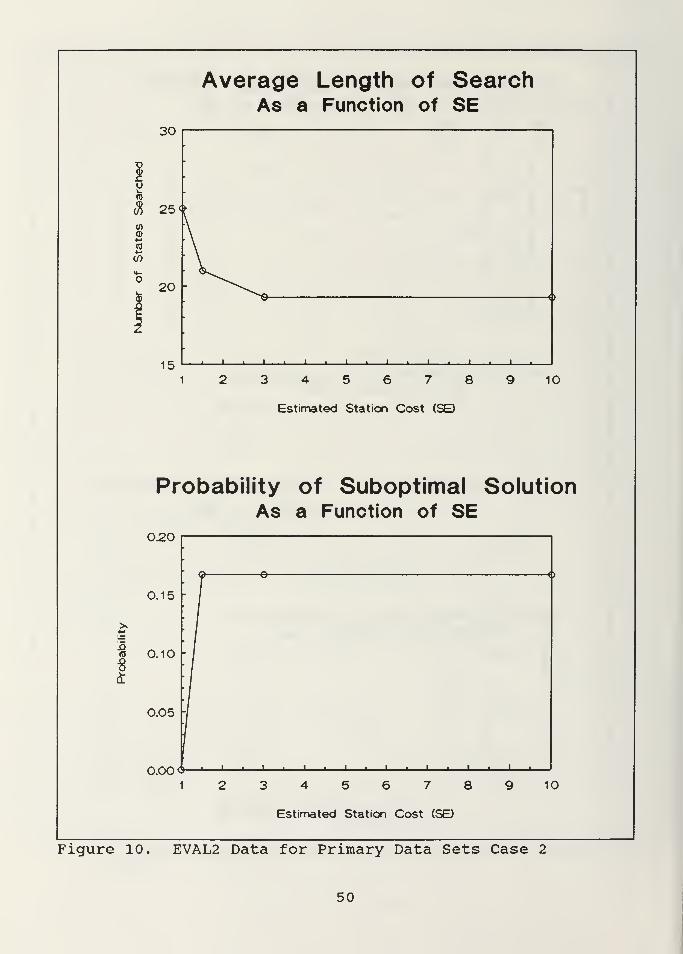
Figure 10 and Figure 11 indicate that the behavior of

EVAL2 is very similar in cases 2 and 3. Although increasing

SE produces a faster search, an optimal solution is only

guaranteed if SE is selected as the minimum cost for an

individual site, exactly as expected.

47

Average Length of SearchAs a Function of SE and log(W2/W1)

-*- SE=1.0

SE= -*- SE= *- SE=1.5 3.0 10.0

"O0)xzo\_(O0)CO

</>

0)

25

20

iS 15CO

o1—

t

10

-* ^

-2.0 -1.0 O.O

log<W2/W 1

)

I.O 2.0

Probability of Suboptimal SolutionAs a Function of SE

0l2O

«J 0. 10

!

123466789 10

Estimated Station Cost <SE)

Probability of Suboptimal SolutionAs a Function of log(W2/W1)

3

0.20

0.15

0.10

0.00-20 -I.O OO

log(W2/W1)to 2.0

Figure 8. EVAL1 Data for Primary Data Sets Case 1

48

Average Length of SearchAs a Function of SE

25

' i ' L

1 23456789 10

Estimated Station Cost (SE)

Probability of Suboptimal SolutionAs a Function of SE

0.20

0.15

ffl 0.10

4

0.05 -

0.00 <»—«—' ' L

1 23456789 10

Estimated Station Cost (SE)

Figure 9. EVAL2 Data for Primary Data Sets Case 1

49

Average Length of SearchAs a Function of SE

30

15 _i i i_ J i I i I i I i L23456789 10

Estimated Station Cost (SE)

Probability of Suboptimal SolutionAs a Function of SE

U^U

0.15

y <J \)

>

(0

Sit

0.10

0.05

' i.i.1 23456789 10

Estimated Station Cost (SE)

Figure 10. EVAL2 Data for Primary Data Sets Case 2

50

Average Length of SearchAs a Function of SE

50

<2 30if)

20

10 J i I i I i L23456789Estimated Station Cost (SE)

10

Probability of Suboptimal SolutionAs a Function of SE

0.50

0.40 -

r 0.305

8t 0.20 -

0.10

0.00*—«

—

L j i i i i i i_ J i L

1 3 4 5 6 7 8 9

Estimated Station Cost (SE)

10

Figure 11. EVAL2 Data for Primary Data Sets Case 3

51

Table IV compares the number of states searched and the

time required for the search for EVAL1 and EVAL2 to that

required by EVAL3 for each of the data sets. These results

demonstrate how effective the heuristic evaluation functions

are in pruning the search space. We set Wl=0.1, and W2=0 . 9 in

EVAL1 and SE=1 . in both EVAL1 and EVAL2, because these values

always produced optimal solutions.

D. SPACE AND TIME USAGE

Table V shows the amount of memory space used by the

program for the various data sets, and the amount of real time

in minutes required to reach a solution. The memory usage for

loading just the Prolog interpreter is 40K, and the memory

used by the interpreter and our program without running any

data sets is 88K.

The memory space used in running the data sets was fairly

uniform, and in all of the cases it was very small compared to

the memory used by the interpreter and the program itself.

The stack usage also varied little. All of the data sets used

close to 64K of global stack and approximately 3K of local

stack.

E. THE SECONDARY DATA SETS

Table VI lists the results of testing the secondary data

sets. These data sets were tested with both EVAL1 and EVAL2

.

We set SE=1 . for these tests because this should guarantee an

52

Table IV. EFFECT OF HEURISTICS ON SEARCH SPACE AND TIME

DATA SETEVAL1:EVAL3 EVAL2:EVAL3

STATES TIME STATES TIME

COAST case 1 0.60 0.44 0.48 0.38

COAST case 2 0.66 0.41 0.66 0.44

COAST case 3 0.35 0.26 0.33 0.23

BAY case 1 0.65 0.51 0.57 0.38

BAY case 2 0.58 0.39 0.50 0.30

BAY case 3 0.36 0.25 0.34 0.24

RIVER case 1 0.66 0.45 0.66 0.45

RIVER case 2 0.92 1.00 0.92 1.00

RIVER case 3 0.36 0.28 0.31 0.22

ISLES case 1 0.77 0.68 0.77 0.68

ISLES case 2 0.91 0.91 0.91 0.89

ISLES case 3 0.78 0.61 0.70 0.50

POINT case 1 0.62 0.29 0.62 0.29

POINT case 2 0.59 0.41 0.59 0.41

POINT case 3 0.40 0.26 0.38 0.24

MIXED case 1 0.50 0.31 0.34 0.14

MIXED case 2 0.85 0.76 0.75 0.55

MIXED case 3 0.41 0.30 0.33 0.19

AVERAGE 0.61 0.47 0.54 0.42

53

Table V. MEMORY USAGE AND RUN TIMES FOR PRIMARY DATA SETS

DATA SETMEMORY (Kbytes) TIME (Minutes)

EVALl EVAL2 EVAL3 EVALl EVAL2 EVAL3

COAST case 1 96 96 108 84 71 189

COAST case 2 92 96 100 34 36 82

COAST case 3 100 104 124 213 190 830

BAY case 1 96 96 108 23 17 45

BAY case 2 92 96 100 30 23 77

BAY case 3 100 104 124 255 243 1019

RIVER case 1 96 96 108 17 17 38

RIVER case 2 92 96 100 18 18 18

RIVER case 3 100 104 128 217 174 785

ISLES case 1 96 96 108 55 55 81

ISLES case 2 92 96 100 32 31 35

ISLES case 3 104 104 128 532 438 879

POINT case 1 96 96 108 11 11 38

POINT case 2 92 96 100 30 30 74

POINT case 3 104 104 128 64 59 247

MIXED case 1 96 96 108 39 18 126

MIXED case 2 96 96 100 70 51 92

MIXED case 3 104 104 128 387 247 1295

54

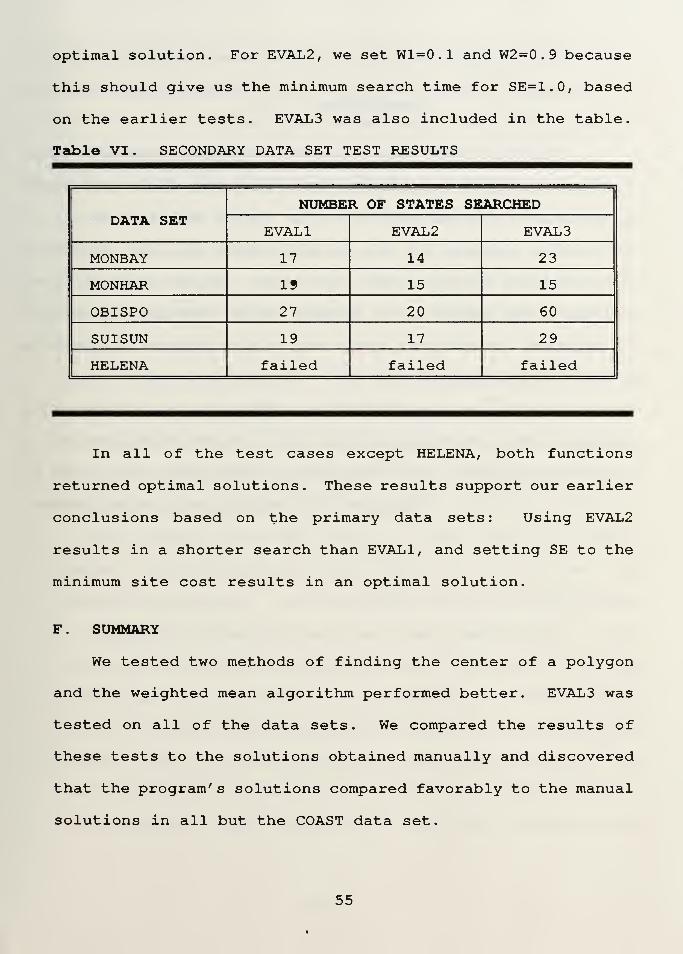
optimal solution. For EVAL2, we set W1=0 . 1 and W2=0 . 9 because

this should give us the minimum search time for SE=1.0, based

on the earlier tests. EVAL3 was also included in the table.

Table VI. SECONDARY DATA SET TEST RESULTS

DATA SETNUMBER OF STATES SEARCHED

EVAL1 EVAL2 EVAL3

MONBAY 17 14 23

MONHAR 15 15 15

OBISPO 27 20 60

SUISUN 19 17 29

HELENA failed failed failed

In all of the test cases except HELENA, both functions

returned optimal solutions. These results support our earlier

conclusions based on the primary data sets: Using EVAL2

results in a shorter search than EVAL1, and setting SE to the

minimum site cost results in an optimal solution.

F. SUMMARY

We tested two methods of finding the center of a polygon

and the weighted mean algorithm performed better. EVAL3 was

tested on all of the data sets. We compared the results of

these tests to the solutions obtained manually and discovered

that the program's solutions compared favorably to the manual

solutions in all but the COAST data set.

55

We then examined the actual successor heuristics used in

the search, and discovered that the heuristics which begin the

search with two sites are not very useful.

EVAL1 and EVAL2 were then tested on the primary data sets

.

EVAL2 resulted in a faster search. Both EVAL1 and EVAL2

returned suboptimal solutions for higher values of SE

.

The pruning of the search space by the heuristic

evaluation functions was discussed. On the average, they

reduce the search space by half while returning an optimal

solution. The memory usage and running time of the program

were also examined.

Finally, we tested EVAL1 and EVAL2 on the secondary data

sets. These test results were very similar to the results of

the primary data set tests. The HELENA data set proved to

have no solution, either with the program or by manual search.

56

VI . CONCLUSIONS

A. GENERAL CONCLUSIONS

Our tests demonstrate the feasibility of using heuristic

search to select sites. With the exception of the COAST data

set, the program's solutions are, on the average, at least as

good as the manual search by a human survey planner. The

memory space used by the program is relatively small and the

search times are fairly reasonable, considering the type of

computer used in testing. The run times would be greatly

reduced by compiling the program and using a better computer

(such as a 386 or 486) with a math coprocessor. In situations

where it is possible to locate sites in a nearly equilateral

triangle, the program performs very well.

The problems with the COAST data set make it clear,

however, that additional work needs to be done on the

successor heuristics. It is difficult to find a good method

of selecting sites for an open coast because it is so

different from an ideal survey situation. Heuristic 7, which

we designed for this case, is not adequate by itself. Both

versions of EVAL3 found much poorer solutions than the manual

search. What is perhaps even more surprising is that, for

case 1 of the COAST data set, version 1 of EVAL3 found a

better solution than version 2. Since it is clear that

57

version 2 employs a better algorithm for finding the center of

a polygon, this may mean that focusing the search on the

center of the remaining survey area is not a good strategy—at

least for the open coast situation. A possible thesis topic

for future students could be the improvement and refinement of

the successor heuristics.

B. ADDITIONAL RELATED WORK

There are many other aspects of survey planning which may

lend themselves to programs of this sort. These include

selecting sites for tide gages; dividing the survey area into

the minimum number of standard sheets; and laying out track

lines for the survey vessel. Finding the optimal path for a

survey vessel to cover a given set of track lines would be

very similar to the classic traveling salesman problem, and

could possibly be solved through a heuristic search or a

simulated annealing technique. These would all make excellent

topics for future theses.

C. MODIFICATIONS TO THE HEURISTIC SEARCH PROGRAM

1 . Shifting Existing Sites

It may be possible to obtain better results from the

program if a successor is generated by shifting one or more of

the sites in an existing state. The problem with this is that

it is seldom clear which sites to shift in what direction to

improve the coverage. If this type of heuristic were used too

58

liberally, the search space would become too large to be

practical. It may be possible to add a post-processing phase

to the program, where the best four or five solutions are

tested to see if they can be improved in this manner.

2 . Fixed Search Space

Instead of using the successor heuristics to limit the

search space, the space can be limited by beginning with a

fixed set of possible station sites, each with a fixed cost

associated with it. A successor would be obtained by adding

any site on the list which is not already in the current

state. The only heuristics employed in this program would be

the evaluation heuristics. This type of program assumes that

a survey team has already performed an initial reconnaissance

of the area, selected a number of possible station sites, and

estimated the relative cost of each site.

3 . Grid Approximation

As mentioned previously, an alternative to

approximating the coverage and survey area with polygons is to

approximate the survey area with a set of grid points. This

method has the advantage of selecting sites based on the

actual horizontal accuracy at each grid point, rather than on

the 30° to 150° coverage circles. Because of this, it would

lend itself easily to other control methods such as range-

azimuth and hyperbolic, and would allow different sites to

have different equipment (with different accuracies)

.

59

The major problem with this method is that it could

require considerably more space and time to run since the grid

must be sufficiently fine to find any coverage gaps. Another

problem is that it would be difficult to apply most of our

successor heuristics (which rely on the center of polygon

function) , and our most important estimation heuristic (which

counts the number of polygons in the remaining survey area)

.

It is possible that different heuristic could be developed for

this case. The successor heuristics could be eliminated

altogether using the fixed search space described above.

D. SUMMARY

It is clear from our tests that the heuristic search

method of selecting sites is feasible. The current program

does, however, have some limitations, and more work is

necessary to make the method practical. This could be the

topic of future theses. We mentioned some additional problems

in survey planning which could also be solved by a heuristic

search program. Finally, we discussed three possible

modifications which could be made to our program.

60

APPENDIX A

THE PRIMARY DATA SETS

The six primary data sets are fictitious areas constructed

to test the program performance in idealized scenarios. They

are COAST, BAY, RIVER, ISLES, POINT, and MIXED, and represent

an open coastline, a bay, a river, a group of islands, a

point, and a mixture of coastline and islands. These six data

sets were each tested under three different cases:

1. The range of the equipment is very long with respect tothe dimensions of the survey and there is no existinggeodetic control in the area.

2. The range of the equipment is long and there are threeexisting geodetic control stations in the area.

3. The range of the equipment is very restricted and thereis no existing geodetic control in the area.

Figure 12 through Figure 2 9 display all eighteen scenarios,

including the program solutions and the manual solutions.

61

CO<cCDCD

COZDCD

CJ

i i i i

csd

csdCSD

in in+3 Qj in• <-\ +-> 111

G--.-M• •—i 1/1 • •—i

•—i inG

>. tn —-+-> oj i_ min > on Z3rd i_ O CZO 3 l_ 03u in o_ e

i D <i

csdCSDcsdCSDCO

CSDcsdCSDCNI

ini_OJ-MQJ

OJen

CH

X

(3D

CSDCSD

J_L '

CSD

CDCSDCSDCSDCO

(X)CSDCSDCSDCN

CSDCSDCSDCSD

CSD

(sja^auj) a&uey ^

Figure 12. COAST Data Set Case 1

62

CO<cCDCJ

COZDCD

CD

CDCDCDcd00

, ,

L_in -m> in

-t-> c qj m.-1 O -*-> CDe LJ -r-l -l->

._, tn —

i

.—i u inh e>» i

•> ro i—

i

-P QJ OJ L TILO > TD CP Z3T3 l_ O O CO D QJ L O]U IT CPQ6

i0° «

CD

CDcd

CD

cdcdCO

ini_QJ+->

CDQJ

CDcd

QJrrCN CP

c£

X

CD

cdcd

JL-L II I I I I I CD

CDCDCDCD

CD

(sja^auj) a&uey ^

Figure 13. COAST Data Set Case 2

63

CO<cCDCD

CO

CD

CJ

IP in-4-S CLI in1—1 +-> CDe i—

i

-m• f—

4

i/i i—

i

,—,e in

>^ rn .—-4-> QJ L_ min > CP =3rd i_ o ao 13 L_ 03o m cl e

• D

I I I I I I II I I

GOISgogo

gogoGOGOCO

ini_QJ-M

GOgo

QJ

CJgoCM QJ

r-rcn

03or

X

(3DCOGOGO

GO

GOGOGOGO00

GOGOGOGOCN

GOGOGOGO

GO

(sja^auj) a&upy ^

Figure 14 . COAST Data Set Case 3

64

DQ

CO

CD

CJ

tn in-M Ql U1• --i -t-s QJ£ -r-. -|-J

• ~J 1/1 -^,—i un

£>-- ra _-.

-M QJ L_ H3in > en =3rO l_ o c:O ZS L_ <T)

lw» Ol CLE

i

D <

' ' ' ' ' ' ' I I I I I I I II I I

(3D

(3D

<3DCSD<3D<X>CO

inL_QJ

-4->

IS)

QJE=

(X)

CM QJ

t=T)CH

X

<S>

<3D

(3D(5)(3D(3D00

(3D(3D(3DCSDCN

(3D(3D(3)C3D

<3D

(sja^aiu) abuey x

Figure 15. BAY Data Set Case 1

65

cd

U>Join -4-> in

cd

+J C QJ Lph O-P (LE l_J •-I -u>

• •—i LTI -—

i

.—i <j in-i e

>^-4—> rfl i—i-P Q) QJ L rUui > "o CP Z3T3 L- O O CO ZJ QJ L_ nd cdu ui CPD.E CD

>-

iOo< *•

@J

CDCDCO

<cQQ

in

CO (U

ZD QJO CDCD e

i—

i

CD\— CD

CM QJena

h- \\

i—

i

\ ',

x X1_L_

\ \

\ -

CD\ CD

% * « CD\ » CD% * -—

i

* *

v *\ •

«

* "

\%% .

%

i i i i i t i i 1 i i i i i i i i i i 1 1 1 T^l 1 1 1

CD CD CD (S)cD cd cdcD cd CDcD CD CDf CM

a&uey y t

Figure 16. BAY Data Set Case 2

66

in en-P QJ Ui.,-H 4-> OJe •-. -mi-h un »i-h

,—l me

>- <T3 —

i

-+^ QJ i__ qjin > cn Z3T> L O Co Z3 L_ T3«-j tn o_ G

i

D *

>-

DQ

COZDCD

CJ

(S>

00

I I I I I I

<s>IS)

<S>

es<3DCO

ini_QJ

-4-J

(3D<S)

OJ

CO<X)CNJ CP

aT3Ctl

X

IS<s<S)

<X)

<SD

(sja^auj) abuey ^

Figure 17. BAY Data Set Case 3

67

in in-+-> Qj in'.-l -4-) Qj

inin

>- hd —

i

-P QJ L TIin > cji z3m i_ o c:O 3 L H3U Ul CLE

D *

C£

CO

CD

C_J

'' i i i i i i

(5)CS

CS>CO

inl_QJ

-»->

QJ

CsJ

CNJQJencTJC£

CS>cs

(3D

CSD

00

CS

CN

CSJGDCS>

CSJ

(Bjaqauj) a&up^j ^

Figure 18. RIVER Data Set Case 1

68

CSD

o \

CSDCSD

L_ I -*ftn+j ip \

-+J C QJ v/i

•--i O -1-5 Qj\

E LJ ..-1 _l_? ! \

• .—i LP ^/

' I

.—i l_> 1/1 / : ' \

..-i e / :

', \

>^-P H3 —- / | \P QJ QJ L H3 ; \

Lfi > "0 CP =3 j I

n) l o o c ' \O 3 Ol L H3 > I CSDU l/i CPQE \ CSD

iOn <

| \ "CSDCSDCO

f \ \:

or / • \ in

LU / \l_QJ

z> / • \ -M1—

1

/ '. \ CSDQJ

Q^ / ': \ _ CSDCSD

CO / i \;

CSDCNJ

OJCP

ZD \ \ \ .

CD \;

/ . eni—

i

\ i / Xi—

i

N. |'

^~ \ :

CJ / :

JCSD

i—

i

/ • 1 <S

LL-

\1

1

CSDCSD

1 1 1 1 / 1 1 1 1 1 1 1 1 1 1 i i i i 1 i i i i i i 1 i i

CSD

CS) CSD CSD CgCSD CSD CSDCSD CSD CSDCSD CSD (X)00 CM """

'

(sja^aiu) a&uey x

Figure 19. RIVER Data Set Case 2

69

<s>in in-P QJ i/i

•H4J Qj i

e --h -+o \ <X>—1 l/l -r—

1

\^

r—. l/l \

'; \

-P QJ L 13 ' \

in > t=n ra '• \

rO i_ O C ! 1

O 13 1^ OJ • \

u in aE • I

:

D 4

\ \ :

CD/ \ — CS)1 \ \ <X>

/ \ \ :

CO

en Y • 1 in

UJ / :, \

i_Qj

z> / • \ 4->

en /

1 \

IS)<3D

QJm

en / 1 \

CSQJen

ZD \% \

O \ / . cc:

i—

i

\\ / ;

X

h— TL_dCJ "-/

\

C5>

Li-

fIn

<S)CD

i i i i / i i i i 1 i i i i i i i i 1 i i i i i i ^ i i cs

es <SD<5> <X>

(S» cg<s>

<s <scs><S>

00 CN "—

'

(sja^auj) a&uey ^

Figure 20. RIVER Data Set Case 3

70

in in-+-> qj un.-i -»j m.—

<

1/1 -i—4

o

QJ

=3 L_

TJen =5O t=

H3u in ae

COLjJ

CO

COZDCD

CJ>

a

d"

Aa

D

o>

a

'''''' I , ' i ' '

CS>

(X)cs(3DCO

eni_QJ-Mdl

CJCS>Csl

QJena<ven

<X>

X

C3

cs>00

<s

CN

CS>CS)

(S»

(sja^auj) a&upy ^

Figure 21. ISLES Data Set Case 1

71

Jm \

a CDCD

in-p in^t*

+j c cu in•^h o -»-» ojG l_l -^H _|_>

.—i un • i—i

i—I l_J U*l

•ph e :

+j qj aj l a] Di r,

:

un > "o cr> 13 :

n3 l_ o a a 1i

O D QJ L nj <X>u in cnCLE

!0<> <

n | : cdGDCO

CO 1 s> ddd

|;

in

LU_l

i_QJ-M

CO :

CDCD

QJ

1—

1

i

—

CO D |

cdCN QJ

CPxz.

CD C£i—

i

X1—i—

i

h-CJ cd1—

1

SB J CDLl

!cs

1 1 1 1 1 1 1 1 1 1 1 1 1 1 1 1 1 1 1 1 1 1 1 1

(X)

CS Q C£> CDS) (5) csCS <X> (X)CS <X> (S)00 CN —

(5ja;aiu) a&upy ^

Figure 22. ISLES Data Set Case 2

72

in in-t-> (U 11*1

•--l -4-> Qi

unin

>-- ro .—

•

-P QJ U T)in > cm 3fO l_ D CO D L T3u in _ e

: o «

COUJ

CO

COIDo

CJ

D

trD

^

aDD

tl

tf

D

D

^1

CO

Q

Csl

mi_QJ

QJ

QJcna<v

x

'' i i i i cs

cs CS> CS»<s (SO cs>cs> <s <X>CS> CD <X>00 CM •—

1

cs>

(sja^auj) a&uey ^

Figure 23. ISLES Data Set Case 3

73

in in-p Qj in• r-t -M CD

>.—• inin

>-. ixi —

i

-P OJ L 03in > cp zina l_ o c=o D l n:u m cl e

i D *

i /i i i i i i i i i i i i i i

gd

G)GD<X>GDCO

inl_GJ-M

G>QJ

G)G)CNI

OJ

aHDCH

X

g>

G>

G)

CDGDGO00

G)G)GDGD

GDG>GDG>

GD

(sja^auj) a&uey ^

Figure 24. POINT Data Set Case 1

74

CDQ-

CO

CD

CJ

, ,

DL_

en -+-» in-m c QJ unh o+^ (Ue U-r-l4->._, m .—i.—i o un

-i e>v_j_? ro i—

i

-P QJ CU L_ TJl/l > "U CP ZJT) L O D CO D QJ L 11U l/i CPQ6

jOn «

I /I I I I I I I I I I I I I I I I II I I I I

COCOCOCO

COCOIS)CDCO

ini_QJ-M

COCO

QJ

COCDCN QJ

CPcnen

X

COcoCOCO

CO

COCOCOCOCO

COCOCOCOCN

COCOCOCO

CO

(sja^auj) a&uey ^

Figure 25. POINT Data Set Case 2

75

CDCj_

CO

CD

CJ

GD<SGDGD

in m-f-3 QJ ini—

i

+-> me • r—

1

-t-»• i—

i

in r—1

1—1£

in

>- TJ ,—

i

-u QJ l_ min > CP =303 L_ a t=o =3 i_ 03lj m cl e

i

<

gd

GDGDCO

gdgd•3DGDCNI

ini_CD

-4->

QJ

QJCPc03en

X

GD

GDIS

U i i i i i i i i i i i i i i i iI I I I I I gd

CDgdgdGD00

GDGDGDGDCM

GDGDGDG)

GD

(5ja^aiu) a&uey ^

Figure 26. POINT Data Set Case 3

76

COCD

<c_JCO

en.

enen<cDQ

CO

O

CJ

I I I I I '

CO

<S>

CSD

CM

CSD(5)IS)

CS)

(3DCO

ini_QJ

-»->

<s>

OJ

CsJ

C»JQJf—

r

in inp Qj inr-i -l-> CU

inin

-P QJ i_ T3m > endra l_ o c=O 13 L_ HDu i/i CLE

: D <

(sja^auj) abuey ^

enc:raen

X

Figure 27. MIXED Data Set Case 1

77

COCD

_JCO

C£

C£c£<cDQ

COIDO

CJ

''''

GOGOGOGOCO

goGOGOGO

GOGOGOCO

inL_QJ-M

GOQJ

GOgo

QJrrc

X

goGOGOGO

in

o

in-p ui-4-> C CD Ul.,-1 o -1-3 QJ

—I 1/1 • r—

I

i—i u m>—»_> rd --.

QJ QJ L_ n3> TO Cn ZJo

QJ rt)

u i/i cn a_ eOn

(5jaj,auj) abuey x

Figure 28. MIXED Data Set Case 2

78

COCD

<c_1CO

C£

GO

CO

O

CJ

' ' 'I'll

CDCDCDCDCO

CDCD(5)<x>CN

CDCDCDCSD

CDCDCDCD

CDCDCSDCDCO

CDCDCDCDCN

CDCDCDCD

un incu in*-> CD

m m

-4-J CDin >TO L_O Z3lj in

TO _l_ TOen =3o c=L_ TOcl e

(sja^auj) abuey x

ini_QJ

CU

QJcn

TOCtl

X

Figure 29. MIXED Data Set Case 3

79

APPENDIX B

THE SECONDARY DATA SETS

The five secondary data sets were taken from actual

charts, and each was tested under its own specific

requirements. MONBAY is a coastal survey of the entire

Monterey Bay. In this survey, medium-range positioning

equipment (ARGO) is used, and no existing geodetic control is

assumed. MONHAR is a survey of Monterey Harbor conducted with

short-range equipment (Miniranger) with several existing

geodetic control stations. OBISPO is a harbor and coastline

survey of San Luis Obispo Bay with short-range equipment

(Miniranger) and no existing control. SUISUN is a channel

survey in Suisun Bay with short-range equipment (Miniranger)

and no control. Finally, HELENA is a survey around the Island

of Saint Helena with short-range equipment (Trisponder) and no

existing control.

Figure 30 through Figure 34 display the five secondary

data sets, with program solutions and manual solutions for all

but the HELENA data set.

80

in unj-> Hi in

in !—

•

in

QJ L_

rao =3 L_

en Z3o c:T3u ui aE

>-

en

>-LU

CD

GDGDGD

G>GDGDGDCO

I I I I I I I I I I I I

in

QJ

rue—

•

G3 C1J

GD CT"G3 czGD ruCM CH

X

GDG3G3GDCO

G3G>GDG>CM

GDG5G3GD

(S3

sja^auj) abuey x

I

Figure 30. MONBAY Data Set

81

enCD

en<c

>-l_Uen

O

, ,

OL_

in-p in-p c oj ini—i o -t-^> die lj 'i-h j->

• —1 1/1 "1—

1

I 1 <w> IPH e^- I > ro r—<

-p m ou l njin > "O en z3T3 l_ O O CO ZS QJ L_ H3U l/i QiQE

I0° «

CNI

CD

00

ini_QJ-MQJ

OJCPc:no

XCDCD

CD

CDcdCDoo

cd(5)cd

CD

sjaqauj) a&uey x

Figure 31. MONHAR Data Set.

82

>-

00

CDQ_CO

DQCD

CO

CO

en

(X)

in

QJ

QJG

QJCPt=mC£

x

in in-4-J QJ in• i—

i

-4-J Qjg i—

i

-»-j

• i—

i

in • i—

i

—*G

in

>- n ,—

i

-4-3 QJ l_ H3in > en 3H3 L_ o Ca =5 i_ TJ<w> in dl e

i n <

<X>

CO

CX)

(5)en

<X>

CO

cs

sja^auj) a&uey x

Figure 32. OBISPO Data Set.

83

DQ

CO

CO

in in-M QJ m•rH -+-> cuG • i—

i

4->•—

i

in • i—

i

r-He

L/l

>- n , 1

-M ai L_ H3IP > cp:rfl i_ o Co =5 i_ roKJ LTI CLE

D <

inl_ai

QJ

CDenaH3

X

CNJ

«s

C5> oCNI

(5ja^auj) a&upy x

Figure 33. SUISUN Data Set

84

U1

LP >

k_» LP

J-L I I I I I I I I I I I I I I I I I I I I I I I I I I I

<3D

in

<X>

cs>Csl * "

<X> in

C\) L_

CO QJ-MQJe—OJCP

<s> 13CXi CH<x> X

<x>

CSD

<53

CO (N

CDcx>(S3(X)

cs>

(sja^auj) a&uey x

Figure 34. HELENA Data Set.

85

APPENDIX C

PROGRAM SOURCE CODE

MODIFIED HEURISTIC SEARCH ALGORITHM

Original Program by Neil Rowe, 1988Modified by Arnold Steed, May 1991

For an application, you must define 5 predicates:(1) successor (State, Newstate)(2) goal_reached (State)(3) eval (State, Evaluation) — estimates cost to goal(4) cost (State, Cost) — computes cost of a state(5) a top-level predicate that initializes things and

calls search

Note: "cost" must be non-negative"eval" should be a lower bound

=======*

,

search (Start , State) :-

clean database,add_st ate (Start)

,

repeat_if_agenda,pick_best_state (State)

,

add_successors (State)

,

retract (agenda (State, _,_) )

,

measure_work

.

pick_best_state (State) :-

asserta (best_state (dummy, dummy) )

,

agenda (S,_, D)

,

best_state (S2,D2)

,

special_less_than (D, D2)

,

retract (best~state (S2, D2) )

,

asserta (best_state (S, D) )

,

fail.pick_best_state (State) :-

best_state (State, D)

,

retract (best_state (State, D) )

,

expunge,not (D=dummy) , !

.

add_successors (State) :-

goal_reached (State) , !

.

add_successors (State) :-

successor (State, Newstate)

,

add_state (Newstate)

,

fail.add_successors (State) :-

retract (agenda (State, C, D) )

,

asserta (used state (State, C) )

,

86

expunge,fail.

add_state (Newstate) :-

cost (Newstate, Cnew) , ! ,

eval (Newstate, Enew) ,

D is Enew + Cnew,asserta (agenda (Newstate, Cnew, D) ) , !

.

add_state (Newstate) :-

not (cost (Newstate, Cnew) )

,

write (' Warning: Your cost function failed on state '),

write (Newstate) , nl, !.

add_state (Newstate) :-

not (eval (Newstate, Enew) ) ,

write (' Warning: Your evaluation function failed on state '),write (Newstate) , nl, !.

repeat_if_agenda

.

repeat_if_agenda :

-

agenda (_,_,_)

,

repeat_if_agenda

.

special_less_than (X, dummy) :-!

.

special_less_than (X, Y) :-

X < Y.

clean_database :

-

abolish ( agenda/3 ),abolish ( used_state/2 ),abolish ( best_state/2 ).

measure_work :

-

count_up (agenda (X, C, D) , NA) ,

count_up (used_state (S, C) , NB)

,

write (NA)

,

write(' incompletely examined state(s) and '),write (NB)

,

write (' examined state(s)'), nl, !.

count_up (P,_) :-

ctr_set (0,0) ,

call( P )

,

ctr_inc (0,_) ,

fail.count_up (_, N) :-

ctr is (0,N) .

87

SURVEY PLANNING PREDICATES

Original Program by Arnold Steed, May 1991

Note: Input data files must have the extension ".dat"and contain the following prolog predicates:

(1) chart_limits ( [Lower_left , Upper_right ] )

(2) shore_line ( Polygon_and_fragment_list )

(3) survey_limits ( Polygon_list )

(4) geodetic_control ( Station_list )

(5) range_limits ( Minimum, Maximum)

(6) site_cost ( Site, Cost )

(7) site deviation ( Floating point number )

plan ( Survey_file, Site_list ):-clean_up,initialize_data ( Survey_file, Area ),search ( [[],_, Area], [Site_list |_] ).

clean_up :—

abolish ( range_constraints/0 ),abolish ( shore_segments/l ), !.

initialize_data ( File, Area ):-

name ( File, Listl ),append ( Listl, ".dat", List2 ),name ( Data_file, List2 ),reconsult ( Data_file ) ,

chart_limits ( Chart )

,

shore_line ( Shore ) ,

trim_shore( Chart, Shore, Trimmed_shore ),asserta( shore_segments ( Trimmed_shore ) ),survey_limits ( Area ) ,

check_range_constraints ( Area ).

trim_shore( [ [XO, YO] , [XI, Yl] ] , Shore, Trimmed_shore ):-

make_segment_list ( [ [ [XO, YO] , [XO, Yl] , [XI, Yl] , [XI, YO] , [XO, YO] ] ]

,

Chart)

,

make_segment_list ( Shore, Seg_shore )

,

trim_outside ( Chart, Seg_shore, Trimmed_shore ), !.

check_range_constraints ( Area ):-

extreme_distance ( Area, Distance ),range_limits ( _, Max ) ,

ifthen( Distance > Max/2,assert (range_constraints) )

.

extreme_distance ( Area, Distance ):—

compress_list_of_lists ( Area, List ),relative distances ( List, , Distance )

.

Define Goal

goal reached ( [ , , []] ) .

88

Define Successors*/

successor ( [_r_r[]] r )'•-

!, fail.successor) [[],_, Area], [Site_pair, C, New_area] ):-

two_initial_sites ( Area, Site_pair ),

find_area_covered ( Site_pair, Area, New_area, A ),C is A/2,

successor) [[],_, Area], [ [Site] , . 0, Area] ):-initial site( Area, Site )

.

successor) [Jsite I List ] , C, Area] , [ [New_site, Site | List ], New_C, New_area] ):

range_const raint s

,

special_site ( Site, New_site ),

valid_site ( New_site, [Site|List] ),

find_area_covered( [New_site, Site | List ] , Area, New_area, A ),length ( [Site | List], N ),Total_area_covered is C*N + A,New_C is Total_area_covered/ (N + 1)

.

successor! [Site_list, C, Area] , [ [New_site | Site_list ] , New_C, New_area] ):-

not ( Site_list = [] ),center_of_area ( Area, Center )

,

choose_one_site ( Center, Site_list, New_site ),find_area_covered ( [New_site | Site_list ] , Area, New_area, A ),length ( Site_list, N ),

Total_area_covered is C*N + A,New_C is Total_area_covered/ (N + 1)

.

two_initial_sites ( Area, Pair ):-

center_of_area ( Area, P0 ),

geodetic_control ( Sites ),find_best_pair ( P0, Sites, Pair ).

two_initial_sites ( Area, Pair ):-

center_of_area ( Area, P0 ),get_radial_intersections ( P0, Intersections ),find_best_pair ( P0, Intersections, Pair )

.

initial_site ( _, Site ):-

geodetic_control ( Sites ),member ( Site, Sites )

.

initial_site ( Area, Site ):-

center_of_area ( Area, Center ),

most_distant_vertex ( Area, Center, Vertex ),find_nearest_shore ( Vertex, Site )

.

initial_site ( Area, Site ):-center_of_area ( Area, Center ),make_segment_list ( Area, Seg_list )

,

nearest_point_on_list ( Seg_list, Center, Point ),find_nearest_shore ( Point, Site ).

choose_one_site ( Center, [Site], New_site ):-

geodetic_control ( [] ),new_site ( Center, [Site], Site, [_,New_site] ).

choose_one_site ( Center, Site_list, 01d_site ):-

geodetic_control ( Control ),setof( Site,

old_site (Center, Site_list, Control, Site) ,

[[_,01d_site] |_] ).choose_one_site ( Center, Site_list, New_site )

:-

member ( 01d_site, Site_list ),setof( Site,

new site (Center, Site list, Old site, Site),

89

[ [_, New_site] |_] )

.

old_site( Center, [Site|List], Control, [Q,01d_site] ):-

member ( 01d_site, Control ),not ( member (01d_site, List) ),pair_quality ( Center, [Site, 01d_site] , Q ),valid_site( 01d_site, [Site|List] ).

new_site( [CX,CY], Site_list, [SX,SY], [Q,Site] ):-

X is CX - (CY - SY)

,

Y is CY + (CX - SX)

,

find_nearest_shore ( [X,Y], Site ),valid_site( Site, Site_list ),

pair_quality ( [CX,CY], [Site, [SX, SY] ] , Q ).new_site( [CX,CY], Site_list, [SX,SY], [Q,Site] )

:-

X is CX + (CY - SY)

,

Y is CY - (CX - SX)

,

find_nearest_shore ( [X,Y], Site ),valid_site( Site, Site_list ),pair_quality( [CX,CY], [Site, [SX, SY] ] , Q ).

new_site( [CX,CY], Site_list, [SX,SY], [Q,Site] ):-

X is SX + 1.5* (SY - CY)

,

Y is SY - 1.5* (SX - CX) ,

find_nearest_shore ( [X,Y], Site ),valid_site( Site, Site_list ),pair_quality( [CX,CY], [Site, [SX, SY] ] , Q ).

new_site( [CX,CY], Site_list, [SX,SY], [Q,Site] ):-

X is SX - 1.5* (SY - CY)

,

Y is SY + 1.5* (SX - CX)

,

find_nearest_shore ( [X,Y], Site ),valid_site( Site, Site_list ),pair_quality ( [CX,CY], [Site, [SX, SY] ] , Q ).

special_site ( Site, New_site ):-

range_limits ( _, Max )

,

R is Max/2,shore_segments ( List )

,

member ( Segment, List ),

seg_circle_intersect ( Segment, [Site,R], New_site ).

find_best_pair ( _, [P1,P2], [P1,P2] ):- !.

find_best_pair ( PO, [Pl|Points], Pair ):-find_best_pair ( PO, Points, Pairl ),find_best_pair2 ( PO, [Pl|Points], Pair2 ),pair_quality ( PO, Pairl, Ql ),pair_quality ( PO, Pair2, Q2 ),ifthenelse( Ql < Q2, Pair = Pairl, Pair = Pair2 ), !.

find_best_pair2 ( _, [P1,P2], [P1,P2] ):- !.

find_best_pair2 ( PO, [PI, P2 IPoints] , Pair ):-

find_best_pair2 ( PO, [PI IPoints], Pairl ),pair_quality ( PO, Pairl, Ql ),pair_quality ( PO, [Pl,P2], Q2 ),ifthenelse( Ql < Q2, Pair = Pairl, Pair = [P1,P2] ), !

pair_quality( PO, [P1,P2], Q ):-

angle_of_intersection ( PI, P2, PO, A ),

Q is (A - pi/2) A 2.

find_nearest_shore ( Point, Site ):-shore_segments ( Shore ) ,

nearest_point_on list ( Shore, Point, Site ), !.

90

Ensure state is not virtually identical to existing state*/

valid_site( Site, Site_list ):-not ( member (Site, Site list) ),sort ( [Sice | Site_listT, Set ),agenda_check ( Set )

,

used_state_check ( Set )

.

agenda_check (Set) :-

agenda ([ S ,_,_],_,_) ,

sort ( S, Set2 )

,

same_set ( Set, Set 2 ), !,

fail.agenda_check (_)

.

used_state_check (Set ):-

used_state ( [S, _,_],_)

,

sort ( S, Set2 )

,

same_set ( Set, Set2 ), !,

fail.used_state_check (_)

.

same_set ( Set_l, Set_2 ):-

site_deviation ( C ),mean_square_error ( points, Set_l, Set_2, E ),E < C.

/'

Survey area coverage

find_area_covered ( Sites, 01d_area, New_area, A ):—

make_segment_list ( 01d_area, Seg_list )

,

set_coverage ( Sites, Seg_list, New_seg_list ),

make_polygon_list ( New_seg_list , New_area ),total_area( Old_area, PA ),total_area( New_area, NA ),A is PA - NA, !

.

network_coverage ( [_] , Area, Area ):- !.

network_coverage ( [Station | Station list], Area, Remaining_area ):-network_coverage ( Station_lisF, Area, New_area ),set_coverage ( [Station | Station_list] , New_area, Remaining_area ), !

set_coverage ( [_] , Area, Area ):- !.

set_coverage ( [Station_l, Station_2 | List ] , Area, Remaining_area ):-

set_coverage ( [Station_l | List ] , Area, New_area ),pair_coverage ( Station_l, Station_2, New_area, Remaining_area ), !.

pair_coverage ( SI, S2, Area, Remaining_area ):-

coverage_parameters ( SI, S2, Rl, R2, M ),check_range ( M, Range )

,

case ( [ Range=short -> simple_coverage (SI, S2, R1,R2,M, Coverage)

,

Range=long -> complex_coverage (SI, S2, Rl, R2,M, Coverage)|no_coverage (Coverage) ] )

,

clip_intersection ( Area, Coverage, Remaining_area ), !.

check_range ( Scale, too_near ):-

range_limits ( Min, )

,

Scale < Min, !

.

check range ( Scale, too far ):-

91

range_limits ( _, Max )

,

Scale > Max, !

.

check_range ( Scale, short ):-range_limits ( _, Max ),

Scale < 0.5*Max, !

.

check_range ( _, long )

.

no_coverage ( [ ] ) .

simple_coverage ( Site_l, Site_2, Rotation_l, Rotation_2, Scale, Coverage ):-check_coverage ( Site_l, Site_2, Side ),

coverage ( Side, Site_l, Site_2, Rotation_l, Rotation_2, Scale, List ),

make_segment_list ( List, Coverage ), !.

complex_coverage ( Site_l, Site_2, Rotation_l, Rotation_2, Scale, Coverage ):-

simple_coverage ( Site_l, Site_2, Rotation_l, Rotation_2, Scale, Max ),

adjust_for_range ( Site_l, Site_2, Max, Coverage ), !.

check_coverage ( SI, S2, Side ):-linear_parameters ( [S1,S2], Baseline ),

survey_limits ( SL ) ,

compress_list_of_lists ( SL, Point_list )

,

check_baseline ( Baseline, Point_list, Side ) , !

.

check_coverage ( _, _, both )

.

check_baseline ( [A,B,C], [[X,Y]], left ):-

approx_less_than( (A*X + B*Y + C) , 0.0 ), !.

check_baseline ( [A,B,C], [[X,Y]], right ):-approx_greater_than( (A*X + B*Y + C) , 0.0 ), !.

check_baseline ( Line, [Point | List ] , Side ):-

check_baseline ( Line, List, Side ), !,

check_baseline ( Line, [Point], Side ).

coverage ( left, Site_l, Site_2, Rotation, _, Scale, [Coverage] ):-coverage_prototype ( Template ),trans form_points ( Template, Site_l, Rotation, Scale, Coverage )

.

coverage ( right, Site_l, Site_2, _, Rotation, Scale, [Coverage] ):-coverage_prototype ( Template )

,

trans form_points ( Template, Site_2, Rotation, Scale, Coverage )

.

coverage ( both, SI, S2, Rl, R2, S, [Coverage_l, Coverage_2] ):-

coverage ( left, SI, S2, Rl, R2, S, [Coverage_l] ),coverage ( right, SI, S2, Rl, R2, S, [Coverage_2] ).

cove rage_pa ramet ers ( Point_l, Point_2, Fwd_az, Back_az, Distance ):-polar_parameters ( Point_l, Point_2, Fwd_az, Distance ),angle_sum( Fwd_az, pi, Back_az ), !.

adjust_for_range ( Site_l, Site_2, Simple_coverage, Coverage ):-

range_polygon ( Site_l, Polygon_l ),range_polygon ( Site_2, Polygon_2 ),polygon_intersection ( Polygon_l, Polygon_2, Range_limit ),polygon_intersection ( Simple_coverage, Range_limit, Coverage ), !.

range_polygon ( Site, Polygon ):-range_limits ( _, Max )

,

range_prototype ( Template ),transform_points ( Template, Site, 0.0, Max, Point_list ),make_segment_list ( [Point_list] , Polygon ), !.

coverage_prototype( [[-0 . 19, . 14 ] , [-0.5,0.88] , [0.0, 1.75]

,

[1.0,1.75], [1.5,0.88], [1.19,0.14], [-0.19,0.14] ]) .

range prototype ([ [1 . 0, . 0] , [0.71,-0.71], [0.0,-1.0], [-0 . 71, -0 . 71]

,

92

[-1.0,0.0], [-0.71,0.71], [0.0,1.0], [0.71,0.71], [1.0,0.0]])

Cost Function

cost ( [Site_li3t ,_,_] , Cost ):-

sum_sites ( Site_list, Sum ),geometry_function ( Site_list, F ),

Cost is Sum + F, !

.

sum_sites ( [], 0.0 ):- !.

sum_sites ( [Site|List], Sum ):-

sum_sites ( List, S ),station_cost ( Site, C )

,

Sum is S + C, ! .

geometry_function ( [], 0.0 ):- !.

geometry_function ( [Site], 0.0 ):- !.

geometry_function ( Site_list, F ):-

relative_distances ( Site_list, Min, Max ),F is 1.0 - Min/Max, !

.

relative_distances ( [P1,P2], D, D ):-!, magnitude( PI, P2, D ).

relative_distances ( [P|List], Min, Max ):-

relative_distances2 ( [P|List], Mini, Maxl ),relative_distances ( List, Min2, Max2 ),ifthenelse ( Mini < Min2,

Min = Mini,Min = Min2 )

,

ifthenelse ( Maxl > Max2,Max = Maxl,Max = Max2 )

.

relative_distances2 ( [P1,P2], D, D ):-

!, magnitude ( PI, P2, D )

.

relative_distances2 ( [PI, P2 | List ] , Min, Max ):-magnitude ( PI, P2, D ),relative_distances2 ( [PI | List], Mini, Maxl ),ifthenelse ( Mini < D,

Min = Mini,Min = D )

,

ifthenelse ( Maxl > D,Max = Maxl,Max = D ) .

93

/ *============== ====== =======—EVALUATION FUNCTION DEFINITIONS

Original code by Arnold Steed, May 1991

Note: Only one of the following functions should bein the database at a time.

/* .

:==*/

/

Heuristic Evaluation Function version 1*/

eval( [[],_,_]' E > :"

!, estimated_site_cost ( Cs ),

E is 2*Cs.eval( [[_],_,_]' E

> :"

! , estimated_site_cost ( E ) .

eval( [_,C,RA] , E ):-

total_area ( RA, A ) ,

Nl is A/C,length ( RA, N2 )

,

evaluation_weights ( Wl, W2 ),estimated_site_cost ( S )

,

ifthenelse ( Nl = err,E is 100.0,E is S*(W1*N1 + W2*N2) ), !.

/*Heuristic Evaluation Function version 2

eval( [[],_,_], E ):-

!, estimated_site_cost ( Cs ),

E is 2*Cs.eval( [[_],_,_], E )

:-

! , estimated_site_cost ( E )

.

eval( [_,C,RA] , E ):-

total_area( RA, A ),Nl is A/C,length ( RA, N2 )

,

estimated_site_cost ( S )

,

ifthenelse ( Nl = err,E is 100.0,(max( [N1,N2], N ), E is S*N) ), !

/*A* Evaluation Function

eval( [_,_, []], ) :- !.

eval ( , 1 )

.

94

CENTER OF POLYGON FUNCTION DEFINITIONS

Original code by Arnold Steed, May 1991

Note: Only one of the following functions should bein the database at a time.

/*Center of Polygonversion 1

7

center_of_polygon ( Polygon, Center ):-

convex_center ( Polygon, Center ).make_segment_list ( [Polygon] , Segment_list )

,

point_in_polygon ( Center, Segment_list ), !.

center_of_polygon ( Polygon, Center ):-

concave_center ( Polygon, Center ).

center_of_polygon ( Polygon, ):—

writeln( 'version 1 of center_of_polygon failed on polygon' ),

signal ( Polygon ),fail.

convex_center ( [_|Polygon], [X,Y] ):-sum_points ( Polygon, X_sum, Y_sum )

,

length ( Polygon, N ),X is integer ( X_sum/N + 0.5 ),Y is integer ( Y_sum/N + 0.5 ), !.

concave_center ( Polygon, Center ):-

largest_triangle ( Polygon, [A, B,C] ), !,

convex_center ( [A,B,C,A], Center ), !.

largest_triangle( [A, B,C,A], [A,B,C] ):- !.

largest_triangle ( [A, B, C | Polygon] , Triangle ):-largest_triangle ( [A, C | Polygon] , New_triangle ),

special_triangle_area ( New_triangle, New_area ),

special_triangle_area ( [A,B,C], 01d_area ),

ifthenelse ( New_area > 01d_area,Triangle = New_triangle,Triangle = [A,B,C] ), !.

sum_points ( [], 0, ):- !.

sum_points ( [ [X, Y] | Points] , X_sum, Y_sum ):-

sum_points ( Points, X_add, Y_add ),X_sum is X + X_add,Y sum is Y + Y add.

/'

Center of Polygonversion 2'/

center_of_polygon ( Polygon, [X,Y] ):-

weighted_sum ( Polygon, Area, X_sum, Y_sum ),X is integer ( X_sum/Area + 0.5 ),Y is integer ( Y_sum/Area + 0.5 ), !.

center_of_polygon ( Polygon, ):-

writeln( 'version 2 of center_of_polygon failed on polygon' ),

signal ( Polygon )

,

fail.

95

weighted_sum( [A, B,A], 0.0, 0, ):- !.

weighted_sum( [A, B, C | Points ] , Area, X_sum, Y_sum ):-weighted_sum ( [A, C |Points] , Part_area, Part_X, Part_Y ),

special_triangle_area ( [A,B,C], Tri_area ),center_of_triangle (

[A,B,C], [Tri_X, Tri_Y] ),

Area is Part_area + Tri_area,X_sum is ?art_X + Tri_area*Tri_X,Y_sum is Part_Y + Tri_area*Tri_Y, !

.

center_of_triangle( [ [XI, Yl] , [X2, Y2] ,[X3, Y3] ] , [X,Y] ):-

X is integer ( (XI + X2 + X3) /3 + 0.5 ),Y is integer( (Yl + Y2 + Y3) /3 + 0.5 ).

96

GEOMETRY PREDICATES

Original Code by Arnold Steed, June 1991Additional Code by Neil Rowe

/*Polygon functions requiring segment-list representation

.*/

polygbn_intersection ( Polygon_l, Polygon_2, Intersection ):-

trim_outside ( Polygon_2, Polygon_l, Trim_list_l ),

trim_outside ( Polygon_l, Polygon_2, Trim_list_2 ),

append ( Trim_list_l, Trim_list_2, Intersection ), !.

polygon_union ( Polygon_l, Polygon_2, Union ):-

trim_inside ( Polygon_2, Polygon_l, Trim_list_l ),trim_inside( Polygon_l, Polygon_2, Trim_list_2 ),append ( Trim_list_l, Trim_list_2, Union ), !.

clip_intersection ( Polygon_to_clip, Test_polygon, Clipped_polygon ):-

triin_inside ( Test_polygon, Polygon_to_clip, Trim_list_l ),

trim_outside ( Polygon_to_clip, Test_polygon, Trim_list_2 ),reverse_direction ( Trim_list_2, Rev_trim_list ),

append( Trim_list_l, Rev_trim_list , Clipped_polygon ), !.

trim_inside( [], Polygon, Polygon ):- !.

trim_inside ( _, [], [] ):- !.

trim_inside( Test_polygon, [Segment | Polygon] , Output_polygon ):-trim_inside( Test_polygon, Polygon, Partial_output ),find_sorted_intersections ( Segment , Test_polygon, Point_list ),trim_inside_segments ( Test_polygon, Point_list, Trim_segments ),append( Trim_segments, Partial_output , Output_polygon ), !.

trim_outside ( [], _, [] ):- !.

trim_outside ( _, [], [] ):- !.

trim_outside ( Test_polygon, [Segment | Polygon] , Output_polygon ):-trim_outside ( Test_polygon, Polygon, Part ial_output ),find_sorted_intersections ( Segment , Test_polygon, Point_list ),trim_outside_segments (Test_polygon, Point_list , Trim_segments) ,

append ( Trim_segments, Partial_output , Output_polygon ), !.

find_sorted_intersections ( Segment, Polygon, Point_list ):-

seg_poly_intersect ( Segment, Polygon, List_l ),linear_parameters ( Segment, Line ),check_endpoints ( Polygon, Line, List_l, List_2 ),sort_intersections ( Segment, List_2, Point_list ), !.

trim_inside_segments ( Test_polygon, [PI, P2 | Point_list ]

,

Segment_list ):-

point_on_polygon ( PI, Test_polygon ),midpoint ( [P1,P2], P ),point_in_polygon ( P, Test_polygon ), !,

trim_segments ( [P2 |Point_list ] , Segment_list ), !.

trim_inside_segments ( Test_polygon, [P |Point_list ] , Segment_list ):-

point_on_polygon ( P, Test_polygon ), !,

trim_segments ( [P |Point_list ] , Segment_list ), !.

trim_inside_segments ( Test_polygon, [P |Point_list ] , Segment_list ):-

point_in_polygon ( P, Test_polygon ), !,

trim_segments ( Point_list, Segment_list ), !.

97

trim_inside_segments ( _, Point_list, Segment_list ):-trim_segments ( Point_list, Segment_list ).

trim_outside_segments ( Test_polygon, [PI, P2 |Point_list ] ,

Segment_list ):-

point_on_polygon ( PI, Test_polygon ),

midpoint ( [P1,P2], P ),

point_in_polygon ( P, Test_polygon ), !,

trim_segmGnts ( [PI, P2 | Point_list ] , Segment_list ), !.

trim_outside_segments ( Test_polygon, [P |Point_list ] , Segment_list )

point_on_polygon ( P, Test_polygon ), !,

trim_segments ( Point_list, Segment_list ), !.

trim_outside_segments ( Test_polygon, [P |Point_list ] , Segment_list )

point_in_polygon ( P, Test_polygon ), !,

trim_segments ( [P | Point_list ] , Segment_list ), !.

trim_outside_segments ( _, [_P |Point_list ] , Segment_list ):-trim_segments ( Point_list, Segment_list )

.

trim_segments ( [], [] ) :- !.

trim_segments ( [_] , [] ):- !.

trim_segments ( [PI, P2 | Point_list ] , [ [PI, P2] | Segment_list ] ):-trim_segments ( Point_list, Segment_list ) .

sort_intersections ( Point_list, [], Point_list ) :- !•

sort_intersections ( [P1,P2], [P3|Points], New_list ):-( same_point ( PI, P3 ) ; same_point ( P2, P3 ) ), !,

sort_intersections ( [P1,P2], Points, New_list ), !.

sort_intersections ( [P1,P2], [P3|Points], New_list ):-

find_points_between ( [P1,P3], Points, List_l ),

find_points_between ( [P3,P2], Points, List_2 ),sort_intersections ( [P1,P3], List_l, Sorted_list_l ),

sort_intersections ( [P3,P2], List_2, [P3 | Sorted_list_2 ] ),

append ( Sorted_list_l, Sorted_list_2, New_list ), !.

find_points_between ( , [], [] ):- !.

find_points_between ( JPlfP2], [P|Points], [P | New_points] ):-between_points ( PI, P2, P ), !,

find_points_between ( [P1,P2], Points, New_points ), !.

find_points_between ( End_points, [_|Points], New_points ):-

find_points_between ( End_points, Points, New_points ).

reverse_direction ( [], [] ):- !.

reverse_direction( [ [PI, P2] | In_list ] , [ [P2, PI] |Out_list ] ):-reverse_direction ( In_list, Out_list ).

/*Line, Segment, and Ray Intersections(polygons represented as segment lists)

7

line_intersection( [A1,B1,C1], [A2,B2,C2], ):-

approx_equal_to ( B1*A2, B2*A1 ), !,

approx_equal_to ( C2*A1, C1*A2 ),approx_equal_to ( C2*B1, C1*B2 ),writeln( 'Warning: Colinear lines may cause errors in polygons.' ),

write_list ( [' Lines :', [Al, Bl, CI] , [A2, B2, C2] ] ),

fail.line_intersection( [A1,B1,C1], [A2,B2,C2], [X,Y] )

:-

D is B1*A2 - B2*A1,X is (C1*B2 - C2*B1)/D,Y is (C2*A1 - C1*A2)/D,ifthen( (X=err; Y=err)

,

(writeln (' Line intersection error.'),

98

writeln( [A1,B1,C1] ),

writeln( [A2,B2,C2] ),fail) ), !.

line_circle_intersect ( [A,B,C], [[XO,YO],R], [X,Y] ):-

approx_equal_to ( B, 0.0 ), !,

X is -C/A,Qa is 1.0,Qb is -2.0*Y0,Qc is (X - X0) A 2 + Y0 A 2 - RA

2,

solve_quadratic ( Qa, Qb, Qc, Y ).line_circle_intersect ( [A,B,C], [[X0,Y0],R], [X,Y] ):-

approx_equal_to ( A, 0.0 ), !,

Y is -C/B,Qa is 1.0,Qb is -2.0*X0,Qc is (Y - Y0) A 2 + X0"2 - RA

2,solve_quadratic ( Qa, Qb, Qc, X )

.

line_circle_intersect ( [A,B,C], [[X0,Y0],R], [X,Y] ):-AB is A/B,Bf is Y0 + C/B,Qa is 1 + AB A

2,

Qb is 2*(AB*Bf - XO)

,

Qc is Bf A 2 + X0 A2 - RA2,

solve_quadratic ( Qa, Qb, Qc, X ),Y is -(A*X + C) /B.

seg_circle_intersect ( [P1,P2], Circle, [X,Y] ):-

linear_parameters ( [P1,P2], Line ), !,

line_circle_intersect ( Line, Circle, [FX,FY] ),between_points ( PI, P2, [FX,FY] ),X is integer ( FX + 0.5 ),Y is integer ( FY + 0.5 )

.

segment_intersection( [P1,P2], [P3,P4], [X,Y] ):-

linear_parameters ( [P1,P2], Line_l ),linear_parameters ( [P3,P4], Line_2 ),line_intersection ( Line_l, Line_2, [FX,FY] ),between_points ( PI, P2, [FX,FY] ),

between_points ( P3, P4, [FX,FY] ),

X is integer ( FX + 0.5 ),Y is integer ( FY + . 5 ) , !.

ray_line_intersect ( Ray, Line, Intersect ):-

ray_to_line ( Ray, Rline ),

line_intersection ( Line, Rline, Intersect ),point_on_ray ( Intersect, Ray ), !.

ray_seg_intersect ( Ray, [P1,P2], [X,Y] ):-linear_parameters ( [P1,P2], Line ),ray_line_intersect ( Ray, Line, [FX,FY] ),between_points ( PI, P2, [FX,FY] ),X is integer ( FX + 0.5 ),Y is integer ( FY + . 5 ) , !.

seg_poly_intersect ( _, [], [] ) :- !.

seg_poly_intersect ( Segment_l, [Segment_2 | Polygon] , [P|Points] )

segment_intersection ( Segment_l, Segment_2, P ), !,

seg_poly_intersect ( Segment_l, Polygon, Points ).seg_poly_intersect ( Segment, [_|Polygon], Points )

:-

seg_poly_intersect ( Segment, Polygon, Points ).

ray poly intersect ( , [], [] ):- !.

99

ray_poly_intersect ( Ray, [Segment | Polygon] , [P|Points] ):-ray_seg_intersect ( Ray, Segment, P ), !,

ray_poly_intersect ( Ray, Polygon, Points )

.

ray_poly_intersect ( Ray, [_|Polygon], Points ):-ray_poly_intersect ( Ray, Polygon, Points )

.

/*Point Location Functions

(polygons are represented as segment lists)*/

point_on_polygon ( Point, [Segment | Polygon] ):-

point_on_segment ( Point, Segment ), !.

point_on_polygon ( Point, [_| Polygon] ):-point_on_polygon ( Point, Polygon ).

point_on_segment ( Point, [Pl,P2] ):-linear_parameters ( [P1,P2], Line ),point_on_line ( Point, Line ),between_points ( PI, P2, Point ), !.

point_on_ray ( P, [P0,Dir] ):-direction( PO, P, PDir ),approx_equal_to ( Dir, PDir ), !.

point_on_line ( [X, Y] , [A, B,C] ):-approx_equal_to ( A*X+B*Y+C, 0.0 ) .

point_in_polygon ( [X,Y], Polygon ):-ray_poly_intersect ( [[X,Y],0.0], Polygon, Point_list ),ray_to_line( [[X,Y],0.0], Line ),

check_endpoints ( Polygon, Line, Point_list, New_list ),length ( New_list, N ),odd ( N ) , !

.

between_points ( [XI, Yl], [X2,Y2], [X,Y] ):-between ( XI, X2, X )

,

between ( Yl, Y2, Y ) , !

.

between ( Nl, N2, N ):-approx_less_than ( Nl, N ),approx_less_than ( N, N2 ) , !.

between ( Nl, N2, N ):-

approx_less_than ( N, Nl ) ,

approx_less_than ( N2, N ) , !.

same_point ( [X,Y], [X,Y] ):-integer ( X ) ,

integer ( Y )

.

midpoint ( [ [XI, Yl] , [X2, Y2] ] , [X,Y] ):-X is integer ( (XI + X2) /2 + 0.5 ),Y is integer ( (Yl + Y2)/2 + 0.5 ).

nearest_point_on_line ( [A,B,C], [X0,Y0], [X,Y] ):-

CO is A*Y0 - B*X0,line_intersection( [A,B,C], [B,-A,C0], [X,Y] ), !.

nearest_point_on_segment ( [P1,P2], PO, [X,Y] ):-

linear_parameters ( [P1,P2], Line ),nearest_point_on_line ( Line, PO, [FX,FY] ),between_points ( PI, P2, [FX,FY] ), !,

X is integer ( FX + 0.5 ),

100

Y is integer ( FY + 0.5 )

.

nearest_point_on_segment ( [P1,P2], P0, P ):-magnitude ( PI, P0, Ml ),magnitude ( P2, P0, M2 ),ifthenelse( Ml < M2, P = PI, P = P2 ) , !

nearest_point_on_list ( [Segment], P0, P ):-

!, nearest_point_on_segment ( Segment, PO, P ).nearest_point_on_list ( [Segment | List ] , PO, P ):-

nearest_point_on_segment ( Segment, PO, PI ),

nearest_point_on_list ( List, PO, P2 ),

magnitude ( PI, PO, Ml ),magnitude ( P2, PO, M2 ),ifthenelse( Ml < M2, P = Pi, P = P2 ) , !.

delete_point ( PI, [PI, P2 IPoints] , Polygon ):-

!, del_one_instance ( PI, Points, Temp ),

append( [P2|Temp], [P2], Polygon ).delete_point ( P, Old_polygon, New_polygon )

:-

del_one_instance ( P, 01d_polygon, New_polygon )

/*Point Transformations

trans form_points ( [], _, _, _, [] ):- !.

trans form_points ( [ [X, Y] |List] , [X0,Y0], Rotation, Scale,[ [XT, YT] |T_list] )

:-

transform_points ( List, [X0,Y0], Rotation, Scale, T_list ),

polar_parameters ( [0,0], [X,Y], Direction, Length ),angle_sum ( Direction, Rotation, Angle ),Magnitude is Length*Scale,XT is integer ( Magnitude*cos ( Angle ) + X0 + 0.5 ),YT is integer ( Magnitude*sin ( Angle ) + Y0 + . 5 ) , !.

/'

Structure Type Conversions

make_segment_list ( [], [] ):- !.

make_segment_list ( [P | Polygons ] , Segment_list ):-

make_segment_list ( Polygons, Segments ),make_segments ( P, S ) ,

append ( S, Segments, Segment_list ), !.

make_segments ( [_] , [] ) :- !.

make_segments ( [PI, P2 IPoints] , [ [PI, P2] | Segments] ):-

make_segments ( [P2 IPoints], Segments ).

make_point_list ( [[P1,P2]], [P1,P2] ):- !.

make_point_list ( [ [PI, P2] | Segments] , [PI, P2 | Points] ):-

find_next_segment ( P2, Segments, New_seg_list ),make_point_list ( New_seg_list, [P2 IPoints] ), !.

find_next_segment ( PI, [ [PI, P2] | Segments] , [ [Pi, P2] | Segments] ):-!find_next_segment ( PI, [Segment | Segments] , New_seg_list )

:-

append( Segments, [Segment], Seg_list ),find_next_segment ( PI, Seg_list, New_seg_list ), !.

make_polygon_list ( Segment_list , Polygon_list ):-

separate_polygons ( Segment_list , Polygon_segments ),make_polygons ( Polygon_segments, Polygon_list ), !.

101

separate_polygons ( [], [] ):- !.

separate_polygons ( [[P1,P2] | Segments],t [ [P1,P2] |Polygon] |Polygons] ):-

separate_one_polygon ( P2, Segments, Polygon, New_list ),separate_polygons ( New_list, Polygons ), !.

separate_one_polygon ( PI, Segments, [ [PI, P2] |Polygon] , Remains )

del_one_instance ( [P1,P2], Segments, New_list ), !,

separate_one_polygon ( P2, New_list, Polygon, Remains ).separate_one_polygon ( _, Segments, [], Segments ).

make_polygons ( [], [] ):- !.

make_polygons ( [Segments | Seg_list] , [Polygon |Poly_list] ):-

make_point_list ( Segments, Polygon ),make_polygons ( Seg_list, Poly_list ), !.

ray_to_line( [[X,Y],D], [A,B,C] ):-A is sin (D)

,

B is -cos (D)

,

C is -(A*X + B*Y) , ! .

/'

Check for Intersections at Vertices'/

check_endpoints ( Polygon, Line, Point_list, New_point_list ):-

multiple_occurance ( Point, Point_list ), !,

member ( [Point_l, Point ] , Polygon ),member ( [Point , Point_2] , Polygon ),check_intersections ( Point_l, Point_2, Line, Flag ),ifthenelse( (Flag > 0),

(del_all_instances ( Point, Point_list, New_list )),(del_one_instance ( Point, Point_list, New_list )) ),

!, check_endpoints ( Polygon, Segment ,New_list, New_point_list )

check_endpoints ( _, _, Point_list, Point_list ).

check_intersections ( [XI, Yl], [X2,Y2], [A,B,C], Flag ):-

Fl is A*X1 + B*Y1 + C,

F2 is A*X2 + B*Y2 + C,Flag is F1*F2, ! .

/'

Area of Polygons(polygons represented as point lists)

total_area( [] , ) :-!

.

total_area( [Polygon | Polygons] , Total_area ):-

total_area ( Polygons, Area_2 ),polygon_area ( Polygon, Area_l ),Total_area is Area_l + Area_2, !

.

polygon_area ( [A,B,A], 0.0 >:- !.

polygon_area ( [A, B, C |Points] , Area ):-

polygon_area ( [A, C I Points] , Part_area ),special_triangle_area ( [A, B, C] , Tri_area ),

Area is Part_area + Tri_area, !

.

special_triangle_area ( [A,B,C], Area ):-

oblique_angle ( A, B, C ), !,

triangle_area ( [A,B,C], Tri_area ),Area is -Tri_area, !

.

special_triangle_area( [A,B,C], Area ):-

102

triangle_area ( [A,B,C], Area ),

triangle_area ( [P1,P2,P3], Area ):-

magnitude ( PI, P2, A ),

magnitude ( P2, P3, B ),magnitude ( P3, PI, C ),

S is (A+B+C)/2,S2 is S*(S-A)*(S-B) *(S-C) ,

Area is sqrt ( S2 ) , !

.

/'

Angle Functions

Original Code by Neil RoweModified by Arnold Steed, June 1991

angle_of_intersection( [XI, Yl], [X2,Y2], [X,Y], Angle ):-

direction ( [X,Y], [XI, Yl], Dl ),

direction ( [X,Y], [X2,Y2], D2 ),

Al is D2 - Dl,smaller_angle ( Al, Angle ), !.

smaller_angle ( Angle, Small_angle ):-A is abs ( Angle )

,

ifthenelse( A > pi,Small_angle is 2*pi - A,Small angle is A ) , !

.

angle_difference ( Al, A2, DA ):-DA12 is Al - A2,normalize_angle ( DA12, DA ),

angle_sum( Al, A2, DA ):-

DA12 is Al + A2,normalize_angle ( DA12, DA )

.

before ( Dl, D2 ):-

angle_difference ( D2, Dl, DT is sin ( D )

,

T >= . , !

.

),

normalize_angle ( A, NA ):-

Twopi is 2*pi,floatmod( A, Twopi, NA ) , !.

find_oblique_angle ( PL, PI, P2, P3 ):-circular_sequence ( PL, PI, P2 ),circular_sequence ( PL, P2, P3 ),oblique_angle ( PI, P2, P3 ) , !.

find_non_oblique_angle ( PL, PI, P2, P3 ):-

circular_sequence ( PL, PI, P2 ),circular_sequence ( PL, P2, P3 ),non_oblique_angle ( PI, P2, P3 ) , !.

circular_sequence ( [PI, P2 | Point_list ] , PI, P2 )

circular_sequence ( [P | Point_list ] , PI, P2 ):-circular_sequence ( Point_list, PI, P2 ).

oblique_angle ( PI, P2, P3 ):-direction( PI, P2, H12 ),direction( P2, P3, H23 ),

103

before ( H12, H23 ) , !

.

non_oblique_angle ( PI, P2, P3 ):-

direction( PI, P2, H12 ),

direction( P2, P3, H23 ),

before ( H23, H12 ) , !

.

/'

Center of largest polygon in list(requires point-list representation)

center_of_area ( Polygon_list , Center ):-

largest_polygon ( Polygon_list, Polygon ),

center_of_polygon ( Polygon, Center ), !.

largest_polygon ( [Polygon], Polygon ):-!.largest_polygon ( [Polyl | List ] , Polygon )

:-

largest_polygon ( List, Poly2 ),polygon_area ( Polyl, Areal ),polygon area ( Poly2, Area2 ),iftheneTse ( Areal > Area2,

( Polygon = Polyl )

,

( Polygon = Poly2 ) ) , !

.

/*Miscellaneous utility predicates

most_distant_vertex ( Polygon_list , Center, Vertex ):-

farthest_in_poly_list ( Polygon_list , Center, Vertex, )

farthest_in_poly_list ( [Polygon], C, P, M ):-

!, farthest_in_point_list ( Polygon, C, P, M ).farthest_in_poly_list ( [Polygon|L], C, P, M )

:-

farthest_in_poly_list ( L, C, PI, Ml ),farthest_in_point_list ( Polygon, C, P2, M2 ),ifthenelse( Ml > M2,

(P = PI, M = Ml) ,

(P = P2, M = M2) ) , ! .

farthest_in_point_list ( [P], C, P, M ):-

magnitude ( P, C, M ) , !.

farthest_in_point_list ( [Pl|Points], C, P, M ):-farthest_in_point_list ( Points, C, P2, M2 ),magnitude ( PI, C, Ml ),ifthenelse( Ml > M2,

(P = PI, M = Ml) ,

(P = P2, M - M2) ) , ! .

get_radial_intersections ( P, I ):-

radial_intersections ( P, 360, I ).

radial_intersections ( P, 0, [] ):- !.

radial_intersections ( P, Dir, I_list ):-

Dir2 is Dir - 20,radial_intersections ( P, Dir2, Part_list ),shore_segments (S)

,

Rad is pi*Dir/180,ray_poly_intersect ( [P,Rad], S, Points ),closest_point ( P, Points, I ),append ( I, Part list, I list ), !.

104

closest_point ( _, [], [] ):-!.closest_point ( _, [P], [P] ):- !.

closest_point ( PO, [Pl|Points], [P] ):-

closest_point ( PO, Points, [P2] ),magnitude ( PO, PI, Ml ),

magnitude ( PO, P2, M2 ),

ifthenelse( Ml < M2, P = PI, P = P2 ),

105

MATH PREDICATES

Original Code by Arnold Steed, May 1991Additional Code by Neil Rowe

min( [X,Y], X ):-

X < Y, ! .

min( [X,Y], Y ):- !

.

min( [X| List] , Min ):-

min ( List , Ml )

,

min( [X,M1] , Min )

.

max( [X, Y] , X ):-

X > Y, ! .

max( [X,Y], Y ):-

!

.

max( [X | List] , Min ):-

max ( List, Ml )

,

max( [X,M1] , Min )

.

approx_less_than ( X, Y ):-

X - Y < (abs(X)+abs(Y) )*1.0e-14, !.

approx_less_than ( X, Y ) :-

X - Y < 1.0e-14

.

approx_greater_than ( X, Y ) :—

Y-X< (abs(X)+abs(Y) )*1.0e-14, !.

approx_greater_than ( X, Y ) :—

Y - X < 1.0e-14

.

approx_equal_to ( X, Y ):-

abs( X - Y ) < (abs(X)tabs(Y) )*1.0e-14, !.

approx_equal_to ( X, Y ):-abs ( X - Y ) < 1.0e-14

.

floatmod( X, M, X ):-

X < M, X >=0, ! .

floatmod( X, M, Y ):-

X<0, !,

MX is - X,floatmod( MX, M, MY )

,

Y is M - MY.floatmod( X, M, Y )

:-

NX is X - M,floatmod ( NX, M, Y ) , !

.

odd( N ):-

integer ( N )

,

(N/2) =\= (N//2)

.

slope_intercept ( [ [XI, Yl] , [X2, Y2] ] , [Slope, Intercept ] ):-

XI =\= X2,Slope is (Y2 - Y1)/(X2 - XI),Intercept is Yl - Slope*Xl.

linear_parameters ( [ [X, Y] , [X, Y] ] , ):-!, write ( 'Warning: Degenerate line at ' ),write ( [X,Y] ),writeln (

' cannot be parametrized.' ),fail.

106

linear_parameters ( [ [XI, Yl] , [X2, Y2] ] , [A,B,C] ):-An is Y2 - Yl,Bn is XI - X2,D is sqrt ( An*An + Bn*Bn )

,

A is An/D,B is Bn/D,C is -(A*X2 + B*Y2)

.

polar_parameters ( [X,Y], [X,Y], 0.0, 0.0 ):- !.

polar_parameters ( [XI, Yl], [X2,Y2], Angle, Magnitude ):-direction ( [XI, Yl], [X2,Y2], Angle ),

magnitude ( [XI, Yl], [X2,Y2], Magnitude ).

direction( [X,Y], [X,Y], _ ):-

write_list ( ['Degenerate line at' , [X, Y],

' has no direction.'] ), nl,

!, fail,direction ( [XI, Yl], [X2,Y2], D )

:-

Y2 < Yl, X2 < XI,direction2( [XI, Yl], [X2,Y2], D2 ),

D is D2 + pi, !

.

direction( [XI, Yl], [X2,Y2], D ):-

Y2 < Yl,direction2( [XI, Yl], [X2,Y2], D2 ),

D is (2*pi) - D2, ! .

direction( [XI, Yl], [X2,Y2], D ):-X2 < XI,direction2( [XI, Yl], [X2,Y2], D2 ),

D is pi - D2, !

.

direction( [XI, Yl], [X2,Y2], D ):-

direction2( [XI, Yl], [X2,Y2], D ), !.

direction2( [XI, Yl], [X2,Y2], D ):-DX is XI - X2, DY is Yl - Y2,ADX is abs(DX), ADY is abs (DY)

,

ADX > ADY, Q is ADY/ADX,D is atan(Q) , !

.

direction2( [XI, Yl], [X2,Y2], D ):-DX is XI - X2, DY is Yl - Y2,ADX is abs(DX), ADY is abs (DY)

,

Q is ADX / ADY,D is (pi/2) - atan(Q) , !

.

magnitude ( [XI, Yl], [X2,Y2], Magnitude ):-DX is X2 - XI, DY is Y2 - Yl,M2 is DXA 2 + DY A

2,

Magnitude is sqrt ( M2 )

.

random_integer ( M, N, R ):-D is N - M + 1,

R is integer ( random*D + M )

.

mean_square_error ( numbers, List_l, List_2, Drms ):-vector_subtract ( List_l, List_2, Residuals ),sum_squares ( Residuals, Sum ),length ( List_l, N )

,

Drms is sqrt ( Sum/N )

.

mean_square_error ( points, List_l, List_2, Drms ):-

position_differences ( List_l, List_2, Residuals ),sum_squares ( Residuals, Sum ),length ( List_l, N )

,

Drms is sqrt ( Sum/N )

.

sum squares ( [], ) :- !.

107

sum_squares ( [X|X_list], Sum ):-Z is X~2,sum_squares ( X_list, A_sum ),

Sum is A_sum + Z

.

position_differences ( [], [], [] ):- !.

position_differences ( [Pl|List_l], [P2|List_2], [M|M_list] )

position_differences ( List_l, List_2, M_list ),

magnitude( PI, P2, M ).

dot_product ( [], [], ) :- !.

dot_product ( [X|X_list], [Y|Y_list], Z ):-dot_product ( X_list, Y_list, Zp ),Z is Zp + X*Y.

scalar_multiply ( _, [], [] ) :- ! .

scalar_multiply( A, [X|X_list], [Y|Y_list] ):-scalar_multiply ( A, X_list, Y_list ),Y is A*X.

vector_add( [], [], [] ):- !.

vector_add( [X|X_list], [Y|Y_list], [Z|Z_list] ):-

vector_add( X_list, Y_list, Z_list ),

Z is X + Y.

vector_subtract ( [], [], [] ):- !.

vector_subtract ( [X|X_list], [Y|Y_list], [Z|Z_list] ):-

vector_subtract ( X_list, Y_list, Z_list ),Z is X - Y.

solve_quadratic ( A, B, C, X ):—

D is B*B - 4*A*C,solve_quadratic ( A, B, C, D, X )

.

solve_quadratic ( _, _, _, D, ):-D < 0, !,

fail.solve_quadratic ( A, B, C, D, X )

:-

approx_equal_to ( D, 0.0 ), !,

X is -B/ (2*A)

.

solve_quadratic ( A, B, C, D, X ):—

X is -(B - sqrt (D) ) / (2*A)

.

solve_quadratic ( A, B, C, D, X ):-X is -(B + sqrt (D) ) / (2*A)

.

108

BASIC PREDICATES

Original code by Arnold Steed, May 1991Additional code by Neil Rowe and Robert Marks

writeln( X ):-

write ( X ) , nl

.

writeln( S, X ):-

write ( S, X ) , nl ( S ) .

write_list ( [] ):-

nl.write_list ( [Element | List ]

):-write ( Element )

,

write (' ' ),

write_list ( List )

.

write_list ( S, [] ) :-

nl ( S ) .

write_list ( S, [Element | List ] ):-write ( S, Element ),write ( S, ' '

) ,

write_list ( S, List )

.

same (X, X )

.

compress_list_of_lists ( [], [] ):- !.

compress_list_of__lists( [List], List ) :- !.

compress_list_of_lists ( [List | Lists] , New_list ):-

compress_list_of_lists ( Lists, Partial_list ),append ( List, Partial_list, New_list ).

list_element ( [Head|_Tail] , Head, 1 ).list_element ( [_Head|Tail] , Element, N )

:-

var( N ),list_element ( Tail, Element, Np ),N is Np + 1

.

list_element ( [_Head|Tail] , Element, N ):-

var ( Element )

,

Np is N - 1,

list_element ( Tail, Element, Np ).

member ( Element, [Element |_List] ).member ( Element, [_Head|Tail] ):-

member ( Element, Tail ).

multiple_occurance ( Element, [Element | List] ):-

member ( Element, List )

.

multiple_occurance ( Element, [_Head|Tail] ):-

multiple_occurance ( Element, Tail ).

del_one_instance ( Element, [Element | List ] , List ).del_one_instance ( Element, [Head | List_l] , [Head | List_2] )

del_one_instance ( Element, List_l, List_2 ).

del_all_instances ( _, [], [] ).del_all_instances ( Element, [Element | Tail] , List )

:-

del all instances ( Element, Tail, List ).

109

del_all_instances ( Element, [Head|Tail_l] , [Head|Tail_2] ):-

del_all_instances ( Element, Tail_l, Tail_2 ).

append ( [], List, List ).append( [Head|Tail], List, [Head |New_t ail] )

:-

append ( Tail, List, New_tail ).

write_current__time ( Time ):-

time ( Time )

,

write_time( Time )

.

write_current_time ( H, Time ):-

time ( Time )

,

write_time( H, Time )

.

write_time( time (H,M, S, HS) ):-Sec is S + HS/100,write

(

H ) , write ( ' :')

,

write

(

M ) , write ( ' :') ,

write

(

Sec )

.

write_time( F, time (H,M, S, HS) ):-

Sec is S + HS/100,write

(

F, H ) , write ( F, ':' ),

write

(

F, M ) , write ( F, ':' ),

write

(

F, Sec )

.

write_current_date ( Date ):-date ( Date )

,

write_date( Date ), !.

write_current_date ( H, Date ):-date ( Date )

,

write_date( H, Date ), !.

write_date( date(Y,M,D) ):-

write

(

M ), write ('-' ),

write

(

D ), write ('-' ),

write

(

Y ) , write ( ''),!.write_date( H, date(Y,M,D) )

:-

write

(

H, M ) , write ( H, '-' ),

write

(

H, D ) , write ( H, '-'),

write

(

H, Y ) , write ( H, ' ') , ! .

elapsed_time ( time (HI, Ml, S1,HS1) , time (H2,M2, S2, HS2) , T ):-HI < H2, !

,

Hp is HI + 24,elapsed_time( time (Hp,Ml, SI, HS1) , time (H2,M2, S2,HS2) , T )

elapsed_time ( Tl, T2, T ):-convert_time( Tl, SI ),convert_time ( T2, S2 ),S is SI - S2,convert_time ( T, S ) .

convert_time( time (H, M, S, HS) , T ):-var(T), !,

T is H*3600 + M*60 + S + HS/100.convert_time ( time (H,M, S, HS) , T )

:-

H is integer (T/3600) ,

M is integer ( (T - H*3600)/60),S is integer(T - (H*3600 + M*60)),HS is integer (100* (T - (H*3600 + M*60 + S) ) )

.

set_global ( Name, Value ):-abolish ( Name/1 ),P=. .

[Name, Value]

,

110

asserta ( P ) , !

.

get_global ( Name, Value ):-

P=. .[Name, Value]

,

call( P ) , !

.

cons_global ( Name, I ):-

P=. .[Name,X]

,

call( P )

,

retract ( P )

,

NP=. . [Name, [I |X] ]

,

asserta ( NP ) , !

.

pop_global ( Name, Value ):-

P=. . [Name, [Value |L] ]

,

call( P )

,

retract ( P )

,

NP=. . [Name,L]

,

asserta ( NP ji , !

.

inc_global ( Name ):-

P=. . [Name,X]

,

call( P )

,

retract ( P )

,

Xpl is X + 1,

NP=. .[Name, Xpl]

,

asserta ( NP ) , !

.

beep:-put (7) .

beep ( N ):-

ctr_set (0,1)

,

repeat,ctr_inc (0,1),[! beep, delay ( 0.25 ) !],I =:= N.

delay ( Seconds ):-

time( time( H, M, S, D ) ) ,

Timel is float (H*3600 + M*60 + S + D/100.0 ),

repeat,time( time( H2, M2, S2, D2 ) ),Time2 is float ( H2*3600 + M2*60 + S2 + D2/100.0 ),Timel + Seconds =< Time2

.

signal ( Message ):-

writeln( Message ), nl,writeln( '< Press any key to acknowledge >' ),repeat,[! beep, delay ( 0.25 ) !],keyb_peek (A, ) ,

getO ( A ) , !

.

Ill

LIST OF REFERENCES

Clark, S. M. , "Hydrographic Survey Planning," notes onbriefing given to prospective Oceanographic Unit commandingofficers, U. S. Naval Oceanographic Office, Stennis SpaceCenter, Mississippi, 13 December 1988.

International Hydrographic Organization (IHO) SpecialPublication No. 44, IHO Standards for Hydrographic Surveys,3rd ed. , International Hydrographic Bureau, 1987.

Kirkpatrick, S., Gelatt Jr, C. D., and Vecchi, M. P.,"Optimization by Simulated Annealing," Science, v. 220, no.4598, pp. 671-680, 13 May 1983.

Laurilla, S. H., Electronic Surveying and Navigation, pp.108-117, John Wiley & Sons, Inc., 1976.

Meridian Ocean Systems, QUILS II Operator' s Manual, p. 57,1989.

Plastock, R. A. , and Kalley, G. , Theory and Problems ofComputer Graphics, pp. 99-104, McGraw-Hill, Inc., 1986.

Rogers, D. F., and Adams, J. A., Mathematical Elements forComputer Graphics, 2nd ed. , pp. 61-100, McGraw-Hill, Inc.,1990.

Rowe, N. C, Artificial Intelligence Through Prolog, pp.191-247, Prentice-Hall, Inc., 1988.

Umbach, M. J., Hydrographic Manual, 4th ed., NationalOceanic and Atmospheric Administration, 1976.

Wells, W. , and Hart, W. W., Plane Geometry, D. C. Heath &

Company, 1915.

112

INITIAL DISTRIBUTION LIST

1. Defense Technical Information CenterCameron StationAlexandria, VA 22304

2. Library, Code 52Naval Postgraduate SchoolMonterey, CA 93943-5000

3. Chairman, Code OC/CoDepartment of OceanographyNaval Postgraduate SchoolMonterey, CA 93943-5000

4. Neil C. Rowe, Code CS/RpDepartment of Computer ScienceNaval Postgraduate SchoolMonterey, CA 93943-5000

5. Everett Carter, Code OC/CrDepartment of OceanographyNaval Postgraduate SchoolMonterey, CA 93943-5000

6. Arnold F. Steed, Code HSANaval Oceanographic OfficeStennis Space CenterMS 39522-5001

7. Director of Naval Oceanography DivisionNaval Observatory34th and Massachusetts Avenue NWWashington, DC 20390

8

.

CommanderNaval Oceanography CommandStennis Space CenterMS 39529-5000

9. Commanding OfficerNaval Oceanographic OfficeStennis Space CenterMS 39522-5001

113

10. Commanding OfficerNaval Oceanographic and AtmosphericResearch LaboratoryStennis Space CenterMS 39529-5004

11. ChairmanOceanography DepartmentU. S. Naval AcademyAnnapolis, MD 21402

12. Chief of Naval Research (Code 420)800 N. Quincy StreetArlington, VA 22217

114

ThesisS67863c.l

SteedA heuristic search

method of selectingrange-range sites forhydrographic surveys.

ThesisS67863c.l

SteedA heuristic search

method of selecting

range-range sites for

hydrographic surveys.