Ecology, 89(8), 2008, pp. 2281–2289� 2008 by the Ecological Society of America

A HIERARCHICAL MODEL FOR SPATIAL CAPTURE–RECAPTURE DATA

J. ANDREW ROYLE1,3

AND KEVIN V. YOUNG2

1U.S. Geological Survey, Patuxent Wildlife Research Center, Laurel, Maryland 20708 USA2Utah State University Brigham City, 265 W. 1100 S., Brigham City, Utah 84302 USA

Abstract. Estimating density is a fundamental objective of many animal populationstudies. Application of methods for estimating population size from ostensibly closedpopulations is widespread, but ineffective for estimating absolute density because mostpopulations are subject to short-term movements or so-called temporary emigration. Thisphenomenon invalidates the resulting estimates because the effective sample area is unknown.A number of methods involving the adjustment of estimates based on heuristic considerationsare in widespread use. In this paper, a hierarchical model of spatially indexed capture–recapture data is proposed for sampling based on area searches of spatial sample units subjectto uniform sampling intensity. The hierarchical model contains explicit models for thedistribution of individuals and their movements, in addition to an observation model that isconditional on the location of individuals during sampling. Bayesian analysis of thehierarchical model is achieved by the use of data augmentation, which allows for astraightforward implementation in the freely available software WinBUGS. We present resultsof a simulation study that was carried out to evaluate the operating characteristics of theBayesian estimator under variable densities and movement patterns of individuals. Anapplication of the model is presented for survey data on the flat-tailed horned lizard(Phrynosoma mcallii ) in Arizona, USA.

Key words: abundance estimation; animal movement models; Bayesian analysis; data augmentation;density estimation; distance sampling; hierarchical modeling; Phrynosoma mcallii; spatial point process;trapping grid; trapping web.

INTRODUCTION

Estimating abundance is a fundamental goal of many

animal sampling problems, and it forms the basis of a

vast body of literature on statistical methods in animal

ecology (e.g., Seber 1982, Williams et al. 2002). An

important consideration in estimating abundance of

most animal populations is that individuals cannot be

observed perfectly. That is, the probability of encoun-

tering or detecting an animal is less than 1.0 in most

survey situations. A number of methods for dealing with

imperfect detection have been devised, including cap-

ture–recapture, its many variations, distance sampling

(Buckland et al. 1993), and approaches that are more

distinctly model based (e.g., Royle and Nichols 2003,

Royle 2004).

However, an equally important component of sam-

pling animal populations is the spatial organization of

sample units, and individuals within the broader

population that is the object of inference. That is, it is

typically not possible to expose all individuals in the

population at large to sampling. Instead, one must

typically delineate sample units (or at least locations)

that will be surveyed.

For example, suppose a 1-ha quadrat is delineated

and surveyed. Animals that are encountered are

uniquely marked, and the survey is repeated a number

of times. It is natural to view the resulting capture–

recapture data as being relevant to some form of a

demographically closed population, provided the sam-

ples were close enough together in time so as to minimize

mortality and recruitment. However, lacking a physical

barrier around the sample plot, there is likely to be

movement of individuals onto and off of the plot,

resulting in a lack of geographical closure. This

phenomenon of temporary emigration (Kendall and

Nichols 1995, Kendall et al. 1997, Kendall 1999) in the

simplest case (random temporary emigration) biases

detection probability (p) low, hence abundance (N)

high. Most importantly, temporary emigration means

that the effective sample area is poorly estimated by the

nominal, delineated area of the sample. That is,

individuals near the borders of the sample unit have

lower exposure to sampling, and those near the interior

have a higher net exposure to sampling. Thus, while we

might have a good quality data set in terms of

information content, we do not know the effective area

from which animals were sampled by the delineated

sample unit. Considerable effort has been focused on the

development of methods for estimating or approximat-

ing the effective sample area. See Parmenter et al. (2003)

for a review of concepts and an extensive evaluation of

some popular methods.

Manuscript received 10 April 2007; revised 19 September2007; accepted 15 November 2007; final version received 19December 2007. Corresponding Editor: B. E. Kendall.

3 E-mail: aroyle@usgs.gov

2281

In this paper, we propose a spatially explicit capture–

recapture model that applies to area-search sampling

wherein a delineated sample unit is searched thoroughly

and all captured animals are uniquely marked. The

process is repeated T times yielding spatially referenced

capture histories on n unique individuals. That is, every

time an individual is captured, a corresponding spatial

location is recorded. Our approach is to parameterize a

hierarchical model in terms of individual activity centers

(which we formally describe mathematically here), and

then a model for individual movement conditional on

the activity centers. Finally, we specify a model for the

observations conditional on the location of individuals

during each sample occasion. The objective is to

estimate absolute density of individuals in the survey

plot. Under our model, this is accomplished by

estimating the number of activity centers contained

within the delineated sample unit. The model is

hierarchical in the sense that a formal distinction is

made (in the model) between the underlying process

model, consisting of the model of individual activity

centers and movement, and an observation model which

describes the detection of individuals during sampling.

When rendered in this way, the model is simple, concise,

flexible, and extensible. We adopt a Bayesian analysis

based on data augmentation (Royle et al. 2007). Using

this approach, the model can be implemented in the

freely available software WinBUGS (Gilks et al. 1994)

with little more than a few lines of ‘‘pseudo-code’’ that

describes the model. The model also produces an

estimate of the relevant ‘‘super-population’’ of individ-

uals that are exposed to sampling. Therefore, the

method allows one to quantify temporary emigration

explicitly without use of the ‘‘robust design’’ (see Pollock

1982, Kendall et al. 1997).

We apply the model to a capture–recapture survey of

flat-tailed horned lizards (Phrynosoma mcallii ) in

southwestern Arizona. This species is difficult to

monitor due to low densities and detection probabilities

(Grant 2005, Grant and Doherty 2007), due in part to its

cryptic coloration and habit of burying under the sand

when approached (Wone and Beauchamp 1995; see

Plate 1). In addition to being difficult to find, these

lizards can move over fairly large distances, and

movement varies annually (K. Young, unpublished data)

and seasonally (Grant and Doherty 2006). Hence, even

when capture–recapture techniques yield an estimate of

p, estimating the effective sample area (and hence actual

density) can be problematic due to movement or

temporary emigration (Grant and Doherty 2007).

MODEL FORMULATION

Suppose that each individual in the population has a

center of activity, or home range center. We will avoid

associating a biological meaning to this concept, but

instead provide a concise mathematical definition. The

home range center for individual i is the point si ¼ (s1i,

s2i ), about which the movements of animal i are

distributed (in a manner to be described precisely)

according to some probability rule.

Thus, si ; i ¼ 1, 2, . . . , N represent the home range

centers for all individuals in the population, which will

be defined to be those individuals within some large

region S that contains the sample unit as a strict subset.

The sample unit (e.g., a transect, plot, or quadrat) will

be denoted by the set D 3 S. We will assume that the siare uniformly distributed over S. In practice, we will

prescribe S (e.g., by specifying coordinates of some

polygon that contains the sample unit). As an example,

consider Fig. 1 (which is described more fully below).

The smaller square is a hypothetical sample unit (i.e., D)

of dimension 10 3 10, and this is nested within a larger

polygon (the dashed line), S, which is a square of

dimension 163 16. The need for a formal definition of S

is related to the construction of the model (described

subsequently). The model postulates, due to movement,

that there are individuals captured having an si that is

located outside of the physical area that was sampled.

The model therefore implies the existence of some S, and

we must choose it to be sufficiently large so that it does

not influence the parameter estimates. More practically,

we specify the model in terms of a point process model

that governs the distribution of the points si, and we

adopt a Bayesian approach to analysis of the model

based on Markov chain Monte Carlo which requires

that we simulate draws of each si from the posterior

distribution. We must therefore describe, explicitly, the

region within which those si are simulated, and that

region is S. Essentially, S is a prior distribution on the

potential location of captureable individuals.

We suppose that an individual moves around

randomly according to some probability distribution

function, g(s; h). We will denote the coordinates at

sample times t as uit ¼ (u1,it, u2,it ) to distinguish them

from the individual centers. In the application below, we

suppose that the random variables (u1, u2) are indepen-

dent normals so that u1,it ; Normal(s1i, r1) and u2,it ;

Normal(s2i, r2). In practice, we do not observe the

individual centers, si, nor do we observe a complete set

of (u1,it, u2,it) pairs for each individual due to imperfect

sampling of individuals. We will describe the model for

the observation process subsequently.

Given the observation model, we will devise the joint

probability distribution of the observations and under-

lying process (the locations of the individuals), and this

will enable us to estimate the number of individual

activity centers located within the sample unit, or in any,

arbitrary region of S.

The observation model

The previous description of the activity centers and

time-specific locations of all individuals in the popula-

tion constitutes the biological process component of the

model. This is the process about which we would like to

learn. As is typical in ecology, we cannot obtain perfect

observations of this process. Instead, we must settle for

J. ANDREW ROYLE AND KEVIN V. YOUNG2282 Ecology, Vol. 89, No. 8

data that arise under some observation model that

induces uncertainty about the underlying state process.

Let y(i, t) be the binary observations indicating

whether individual i is encountered during sample t

[y (i, t) ¼ 1] or not [y (i, t) ¼ 0]. In practice, we obtain

these encounter histories on i ¼ 1, 2, . . . , n � N

individuals, which we will organize in the array Yn3T. In

addition to these encounter histories, there is a

corresponding pair of coordinates uit ¼ (u1,it, u2,it ) for

each occasion in which individual i was captured. We

emphasize that the sample method addressed here is an

‘‘area search’’ and so these observed coordinates may be

anywhere in D. They are not restricted to locations that

correspond to trap locations. We require an observation

model that describes the manner by which the uit pairs

are observed. We only observe uit whenever y (i, t) ¼ 1.

Otherwise, the uit will be viewed as missing data.

The observation model is derived as follows. If uit is

contained in D during the survey at t, then individual i is

detected with probability p. Otherwise, the individual

cannot be detected and y (i, t) ¼ 0 with probability 1.

That is, y (i, t) is a deterministic zero in this case. These

two possibilities are manifest precisely in the following

model for the observations:

yði; tÞ ¼ 0 if uit =2 D

yði; tÞ; Bernoulli½ pði; tÞ� if uit 2 D:

As described here, we have assumed no behavioral

response to capture (e.g., trap happiness or trap shyness),

which we feel is sensible for the lizard survey described in

Flat-tailed horned lizard data, which are captured by

hand during an exhaustive area search by crews of

several individuals. However, we have the usual flexibil-

ity for modeling p(i, t), for example as a function of time

or covariates, where such considerations are relevant.

This model is a special case of what are usually

referred to as ‘‘individual covariate’’ models (see Pollock

2002). The individual covariate in this case is si, and it is

unobserved. Secondly, this model is a model of

temporary emigration, under a more general form of

temporary emigration than random temporary emigra-

tion considered by Kendall (1999).

Illustration: simulated data

Fig. 1 shows an example of a realization from the

process model described above and the resulting pattern

of observations. As noted previously, the sample unit is

a square of dimension 10 3 10 units, and this is nested

FIG. 1. Simulated 10 3 10 sample unit nested within S, a 16 3 16 square, containing 200 individual activity centers (redtriangles) of which 46 are contained within the sample unit. The large and small black dots are all locations of each individual foreach of T¼ 5 hypothetical survey occasions. The large black dots correspond to capture locations.

Month 2008 2283SPATIAL CAPTURE–RECAPTURE MODELS

within S, a larger square of 163 16 units. We simulated

N¼200 individuals and subjected them to sampling with

p¼ 0.25. Their movement was bivariate normal with r1

¼ 1 and r2 ¼ 1. The small and large black dots are all

locations of each individual for each of T ¼ 5

hypothetical survey occasions (some of which are not

captures). The large black dots were the actual capture

locations within the sample unit.

In all, 81 of the 200 individuals had their center of

activity (red triangles) within the sample unit. A total of

57 individuals were observed in the sample, and this

included 46 individuals having their center of activity

within the sample unit. The remaining 11 captured

individuals were among the 119 having their centers

outside of the sample unit. The 57 captured individuals

were observed a total of 76 times during the five samples,

with p ¼ 0.25.

The statistical objective is to estimate the number of

centers within the 103 10 sample unit, when confronted

only with the capture histories of the 57 individuals, and

the locations of the large black circles in Fig. 1. In the

following Section, we describe a Bayesian analysis of

this model, and its implementation in WinBUGS.

BAYESIAN ESTIMATION BY DATA AUGMENTATION

The model is a specialized case of the individual

covariate models, wherein the individual effect is latent

(i.e., unobserved). Analysis of the classical individual

covariate or heterogeneity models using likelihood

methods is relatively straightforward integrated likeli-

hood (e.g., Coull and Agresti 1999, Dorazio and Royle

2003, Royle 2008). However, it is not immediately

apparent how to carry out such an analysis in the

present problem. In particular, the location of individ-

uals at each sample occasion are realizations of a

partially observed random variable, and they must be

removed from the conditional likelihood by integration.

Alternatively, Bayesian analysis can be accomplished

very directly using methods of Markov chain Monte

Carlo (MCMC). Within the MCMC framework, the

unobserved locations are removed by Monte Carlo

integration thus avoiding the necessity of explicit

integration. We adopt a general strategy here based on

a method of ‘‘data augmentation’’ (Tanner and Wong

1987). Here, we will avoid the technical details which

justify the following, instead focusing on its heuristic

motivation and practical implementation. The mathe-

matical justification for a related class of models is given

in Royle et al. (2007).

Data augmentation can be formally motivated by the

assumption of a discrete uniform prior on N having

support on the integers N ¼ 0, 1, . . . , M for some large

M. Under a reparameterization, the model is equivalent

(Royle et al. 2007) to physically augmenting the

observed data set with a large number, M � n, of ‘‘all

zero’’ encounter histories. Thus, the size of the data set

(M ) becomes a fixed quantity, and the model is

reparameterized to be technically equivalent to what

are sometimes referred to as ‘‘site occupancy’’ models

(e.g., MacKenzie et al. 2006). While the technical

derivation is precise, the augmented zeros are something

of an abstraction, corresponding to what one might call

‘‘pseudo-individuals,’’ only a subset of which are

members of the population of size N that was exposed

to sampling. We assert thatM is sufficiently large so that

the posterior of N is not truncated (this can be achieved

by trial and error with no philosophical or practical

consequence). Given the augmented data set, we now

introduce a latent indicator variable, say zi; i¼ 1, 2, . . . ,

M, such that zi ¼ 1 if the ith element of the augmented

list is a member of the population of size N, and zi ¼ 0

otherwise. We impose the model zi ; Bernoulli(w),where w will be referred to as the inclusion probability.

This is the probability that an individual on the list of

pseudo-individuals is a member of the sampled popula-

tion of size N. Under this formulation, the resulting

model is a zero-inflated version of the ‘‘known-N’’

model, which provided some of the motivation under-

lying the formulation put forth by Royle et al. (2007).

Specifically, 1� w is the zero-inflation parameter, and wis related to N in the sense that N ; Binomial(M, w)under the model for the augmented data. This relation-

ship between N and w has been noted elsewhere in the

context of site occupancy models and closed population

size estimation (Karanth and Nichols 1998, Royle et al.

2007).

While developing the MCMC algorithm for analysis

of the augmented data is straightforward under this

model, we avoid those technical details because the

model can also be implemented directly in WinBUGS,

which is the approach adopted here. We provide the

WinBUGS implementation in the Supplement so that

readers may experiment with the model and its analysis

under various scenarios. Some results of simulations are

provided in the following section.

MCMC methods obtain a sample of the model

parameters from the posterior distribution by Monte

Carlo simulation. Typically, a large sample of dependent

draws from the posterior is obtained after an initial

sample (referred to as the ‘‘burn-in’’) is discarded to

ensure that subsequent draws are being generated from

the target distribution. There are many practical aspects

to Bayesian analysis and MCMC which are discussed

extensively in a large number of recent publications

including the WinBUGS manual (Gilks et al. 1994), and

recent review articles including Link et al. (2002) and

Ellison (2004).

Within the MCMC framework, the individual activity

centers are regarded as missing observations, and they

are estimated by Monte Carlo sampling from the

posterior distribution. That is, we obtain a sample of

each sðjÞi for Monte Carlo iterations j¼ 1, 2, . . . . Various

estimands of interest are derived parameters under the

model formulation put forth here. For example, the

parameter N is the number of individual centers in the

region S, and this is obtained by calculating RMi¼1 zi for

J. ANDREW ROYLE AND KEVIN V. YOUNG2284 Ecology, Vol. 89, No. 8

each iteration of the MCMC algorithm. Similarly, the

number of centers within the sample unit, N(D), and the

density of individuals (which is just a scaled version of

N(D)), are derived parameters, which can be computed

from the posterior draws of the individual activity

centers. That is, we tally up those activity centers which

are within D during each iteration of the MCMC

algorithm. Our WinBUGS model specification does this

explicitly using the WinBUGS model specification

syntax (see Supplement).

EXAMPLES

Simulated data

The model was fit to the data set described in

Illustration: simulated data. Recall that 81 of the 200

individuals had their center of activity within the sample

unit, and, with p ¼ 0.25, a total of 57 individuals were

observed in the sample, including 46 of those 81

individuals having their center of activity within the

sample unit.

The posterior mean (SD; 95% confidence interval) of

N(D) was 79.06 (12.84; 59–109). For the detection

probability, the posterior mean was 0.200 (0.036; 0.134–

0.275). The posterior means (SD) of r1 and r2 were

0.962 (0.039) and 1.054 (0.051), respectively. In this case,

r1 ’ r2, consistent with the data-generating model in

which the two variance components were both set to 1.0.

We expanded our use of simulated data under more

variable conditions by considering populations having r2 f1, 2, 4g, five levels of density (see Table 1), while

keeping the 103 10 unit sample area fixed and p¼ 0.25.

The range of densities correspond to population sizes

within the 100 unit2 sample area of roughly 23–78.

Summary statistics of populations under these scenarios

are given in Table 1. We note that the average p of

individuals in the population is only 0.023 for r¼ 4 and

increases to only 0.098 for r ¼ 1. These are extraordi-

narily low detection probabilities and we therefore

believe the results of the density estimator should reflect

worst-case scenarios. In particular, when the movement

parameter is r¼ 4, we expect to capture only about 10%

of the individuals in the population (with T ¼ 5) and

only about 10% of those are captured more than one

time.

For each level of density (five levels) and r (three

levels), we simulated 100 data sets to which the model

was fitted in WinBUGS based on 10 000 post burn-in

draws from the posterior. Summaries of the estimated

density (posterior mean) across all 100 replicates for

each of the 15 cases are given in Table 2. We have

provided the mean, median, and standard deviation

across replicates as well as the coverage of a nominal

95% posterior interval, which was computed as the 2.5th

and 97.5th percentiles. As expected (i.e., in small

samples), the estimator appears slightly biased, and the

bias is more pronounced for the lower density situations

due to the very small sample sizes (see Table 1). We note

that the bias diminishes rapidly from about 15% to

about 4% as density increases from the lowest level

(0.234) to the highest (0.781). We see that the mean and

median are not too different, and typically close to the

data-generating value. The bias affects the confidence

interval coverage (mostly at the lower value of r),generating a typical coverage (averaged across levels of

density) close to 90% for r ¼ 1 and r ¼ 2, and then

about 96% for the high-movement case.

Flat-tailed horned lizard data

Here we apply the model to estimate the density of the

flat-tailed horned lizard in southwestern Arizona from a

TABLE 1. Summary of encounter history frequencies, expected number of individuals captured (E [n]), and mean detectionprobability (E [p]) for individuals in simulated populations.

r Density

Encounter frequency distribution

0 1 2 3 4 5 E [n] E [p]

4 0.234 0.900 0.085 0.013 0.001 0 0 27 0.0234 0.352 0.902 0.082 0.015 0.002 0 0 40 0.0234 0.469 0.900 0.085 0.013 0.002 0 0 54 0.0234 0.586 0.903 0.083 0.013 0.001 0 0 66 0.0234 0.781 0.902 0.083 0.013 0.001 0 0 88 0.0232 0.234 0.713 0.209 0.063 0.014 0.001 0 33 0.0772 0.352 0.716 0.205 0.063 0.014 0.002 0 48 0.0772 0.469 0.711 0.211 0.062 0.014 0.001 0 66 0.0772 0.586 0.713 0.205 0.065 0.015 0.002 0 81 0.0772 0.781 0.709 0.211 0.064 0.015 0.001 0 110 0.0771 0.234 0.668 0.214 0.093 0.022 0.003 0 20 0.0981 0.352 0.669 0.209 0.091 0.027 0.003 0 30 0.0981 0.469 0.665 0.215 0.091 0.025 0.004 0 40 0.0981 0.586 0.662 0.216 0.092 0.026 0.004 0 51 0.0981 0.781 0.665 0.212 0.095 0.024 0.003 0 67 0.098

Notes: Populations were simulated under five levels of density, with movement rate parameter r 2 f1, 2, 4g. Density is thenumber of individuals per unit area; encounter history frequency distribution is the probability that an individual is captured 0, 1, 2,3, 4, or 5 times. Individuals in simulated populations had home range centers within 2 SE of the trapping grid, and were subject toencounter on a 10 3 10 unit area.

Month 2008 2285SPATIAL CAPTURE–RECAPTURE MODELS

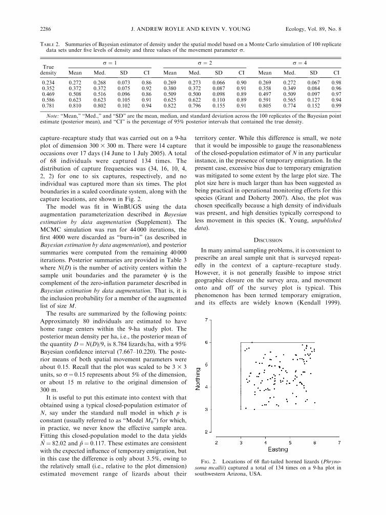
capture–recapture study that was carried out on a 9-ha

plot of dimension 300 3 300 m. There were 14 capture

occasions over 17 days (14 June to 1 July 2005). A total

of 68 individuals were captured 134 times. The

distribution of capture frequencies was (34, 16, 10, 4,

2, 2) for one to six captures, respectively, and no

individual was captured more than six times. The plot

boundaries in a scaled coordinate system, along with the

capture locations, are shown in Fig. 2.

The model was fit in WinBUGS using the data

augmentation parameterization described in Bayesian

estimation by data augmentation (Supplement). The

MCMC simulation was run for 44 000 iterations, the

first 4000 were discarded as ‘‘burn-in’’ (as described in

Bayesian estimation by data augmentation), and posterior

summaries were computed from the remaining 40 000

iterations. Posterior summaries are provided in Table 3

where N(D) is the number of activity centers within the

sample unit boundaries and the parameter w is the

complement of the zero-inflation parameter described in

Bayesian estimation by data augmentation. That is, it is

the inclusion probability for a member of the augmented

list of size M.

The results are summarized by the following points:

Approximately 80 individuals are estimated to have

home range centers within the 9-ha study plot. The

posterior mean density per ha, i.e., the posterior mean of

the quantity D¼N(D)/9, is 8.784 lizards/ha, with a 95%

Bayesian confidence interval (7.667–10.220). The poste-

rior means of both spatial movement parameters were

about 0.15. Recall that the plot was scaled to be 3 3 3

units, so r¼ 0.15 represents about 5% of the dimension,

or about 15 m relative to the original dimension of

300 m.

It is useful to put this estimate into context with that

obtained using a typical closed-population estimator of

N, say under the standard null model in which p is

constant (usually referred to as ‘‘Model M0’’) for which,

in practice, we never know the effective sample area.

Fitting this closed-population model to the data yields

N̂¼ 82.02 and p̂¼ 0.117. These estimates are consistent

with the expected influence of temporary emigration, but

in this case the difference is only about 3.5%, owing to

the relatively small (i.e., relative to the plot dimension)

estimated movement range of lizards about their

territory center. While this difference is small, we note

that it would be impossible to gauge the reasonableness

of the closed-population estimator of N in any particularinstance, in the presence of temporary emigration. In the

present case, excessive bias due to temporary emigration

was mitigated to some extent by the large plot size. The

plot size here is much larger than has been suggested asbeing practical in operational monitoring efforts for this

species (Grant and Doherty 2007). Also, the plot was

chosen specifically because a high density of individualswas present, and high densities typically correspond to

less movement in this species (K. Young, unpublished

data).

DISCUSSION

In many animal sampling problems, it is convenient toprescribe an areal sample unit that is surveyed repeat-

edly in the context of a capture–recapture study.

However, it is not generally feasible to impose strictgeographic closure on the survey area, and movement

onto and off of the survey plot is typical. This

phenomenon has been termed temporary emigration,and its effects are widely known (Kendall 1999).

TABLE 2. Summaries of Bayesian estimator of density under the spatial model based on a Monte Carlo simulation of 100 replicatedata sets under five levels of density and three values of the movement parameter r.

Truedensity

r ¼ 1 r ¼ 2 r ¼ 4

Mean Med. SD CI Mean Med. SD CI Mean Med. SD CI

0.234 0.272 0.268 0.073 0.86 0.269 0.273 0.066 0.90 0.269 0.272 0.067 0.980.352 0.372 0.372 0.075 0.92 0.380 0.372 0.087 0.91 0.358 0.349 0.084 0.960.469 0.508 0.516 0.096 0.86 0.509 0.500 0.098 0.89 0.497 0.509 0.097 0.970.586 0.623 0.623 0.105 0.91 0.625 0.622 0.110 0.89 0.591 0.565 0.127 0.940.781 0.810 0.802 0.102 0.94 0.822 0.796 0.155 0.91 0.805 0.774 0.152 0.99

Note: ‘‘Mean,’’ ‘‘Med.,’’ and ‘‘SD’’ are the mean, median, and standard deviation across the 100 replicates of the Bayesian pointestimate (posterior mean), and ‘‘CI’’ is the percentage of 95% posterior intervals that contained the true density.

FIG. 2. Locations of 68 flat-tailed horned lizards (Phryno-soma mcallii) captured a total of 134 times on a 9-ha plot insouthwestern Arizona, USA.

J. ANDREW ROYLE AND KEVIN V. YOUNG2286 Ecology, Vol. 89, No. 8

Unfortunately, it has not generally been possible to

account for temporary movements in the absence of

additional information such as replicate surveys carried

out under the so-called ‘‘robust design’’ (Kendall et al.

1997). This notion has been used in other herptile

surveys by Bailey et al. (2004a, b), and the basic concepts

and existing methods have recently been reviewed by

Parmenter et al. (2003).

In this paper, we described a hierarchal model of the

temporary emigration phenomenon that is informed by

location-of-capture information. The model is hierar-

chical in the sense that it is comprised of an explicit

process model, and an observation model that is

conditional on the underlying state process. The process

model describes the spatial organization of home-range

centers, and the movement of individuals over time. The

observation model describes the probability of encoun-

ter as a function of an individual’s location at the time of

sample, and a probability of detection parameter.

Bayesian analysis of this hierarchical analysis is

straightforward with the aid of data augmentation

(Royle et al. 2007). Under data augmentation, the

TABLE 3. Parameter estimates for the lizard data.

Parameter

Posterior percentiles

Mean SD 2.5% 50% 97.5%

N(D) 79.23 5.947 69.0 79.0 92.000b 8.784 0.659 7.667 8.667 10.220p 0.122 0.013 0.097 0.121 0.149r1 0.154 0.011 0.136 0.153 0.176r2 0.150 0.001 0.133 0.150 0.172w 0.626 0.077 0.483 0.626 0.781

Notes: N(D) is the number of home range centers located within the 9-ha study plot, and b is theestimated density (no. individuals/ha). The parameter w is the zero-inflation parameter, which isrelated to the total population of exposed individuals as described in Bayesian estimation by dataaugmentation.

PLATE 1. Not only does the flat-tailed horned lizard (Phrynosoma mcallii ) match the color of its sandy habitat, but it typicallypresses against or buries under the sand rather than fleeing, adding to the difficulty of detecting this species. Photo credit: K. V.Young.

Month 2008 2287SPATIAL CAPTURE–RECAPTURE MODELS

observed sample of size n is physically augmented with a

large number of all-zero encounter histories. This leads

to a reparameterization of the model: the resulting

model being a zero-inflated version of the ‘‘known N’’

model. That is, the reparameterized model explicitly

admits that the augmented data set contains an excess of

zeros. Data augmentation was devised as a method for

facilitating the Bayesian analysis of models with

individual effects of which the present model is a

specialized case, having an individual effect (individual

activity center) that is not observed. One of the

important advantages of data augmentation is that it

yields a fairly accessible implementation by MCMC.

The model proposed here can be implemented directly in

WinBUGS with little difficulty.

In the flat-tailed horned lizard example, the method

was used to obtain an estimate of density that allows for

bias due to movement of individuals into and out of the

sample plot. The typical movements (embodied in the

parameter r) were found to be small relative to the total

plot dimension (r̂¼ 0.15 relative to a standardized plot

dimension of three units). This was expected to a certain

extent as the large plot size was chosen in part to

minimize the effects of temporary emigration. However,

in general, there could be some advantage to using plots

of smaller size (e.g., more plots could be sampled,

thereby achieving more diverse landscapes and hence a

more representative sample), in which case the effects of

movement would be more acute. In such cases, there

would probably be a need to model additional structure

in the parameter r as home-range size would be

expected to change in response to density and local

conditions (e.g., see Discussion in Grant and Doherty

2007). The flat-tailed horned lizard is a difficult species

to monitor because of its low detection probabilities,

which are due, in part, to movement or temporary

emigration. The method presented here provides an

alternative to conventional methods (capture–recapture

and distance sampling) that allows for temporary

emigration and enables sampling on arbitrary plot sizes.

Using simulation studies, we evaluated the perfor-

mance of the proposed estimator under situations in

which the movement-to-plot-dimension ratio was con-

siderably larger than for the flat-tailed horned lizards.

For a 10 3 10 unit plot, we considered r 2 f1, 2, 4g,which is approximately 23, 43, and 83 the movement-

to-plot-dimension ratio found in the lizard data. These

simulations suggested tolerable levels of small-sample

bias (5–15%) in the estimator (posterior mean) even

under situations for which typical data sets contain few

individuals captured more than one time (see Table 1).

There are a number of conventional solutions for

obtaining estimates of density when the effective trap

area is unknown, or the study is subject to temporary

emigration. Some of these involve modification of the

basic survey method and design from conventional

capture–recapture methods (e.g., distance sampling

[Buckland et al. 1993], or trapping grids [Wilson and

Anderson 1985b]), while others involve various adjust-

ments to the nominal plot area (e.g., by the radius of a

home range [Otis et al. 1978] or by mean maximum

distance moved [Wilson and Anderson 1985c]), or the

use of ‘‘nested grids’’ (Wilson and Anderson 1985a).

These adjustments are used in camera trap surveys of

tigers in India (Karanth and Nichols 1998, Nichols and

Karanth 2002), small mammal trapping (Parmenter et

al. 2003), and in many other settings. Another form of

adjustment is based on auxiliary data from telemetry

information (White and Shenk 2001) when it is practical

to obtain such information. Oftentimes, however,

information necessary to apply such adjustments is

obtained from the literature on the species in question,

i.e., from prior, similar studies. The problem with the

use of such prior information is that the estimate used to

formulate the adjustment comes from somewhere else—

some other place, some other time, under different

conditions. That is, a different population of individuals.

Thus, the estimate of density for the population under

study is only as good as the relevance of the extrinsic

estimate of home range size which cannot be assessed, in

general, and likely varies in response to a host of factors.

On the other hand, the method that we have described

produces an ‘‘adjustment’’ that is intrinsic to the data set

at hand, i.e., the same data set that produces the

estimate of N. While this is immediately useful for

obtaining estimates of density of the population under

study, the model also allows for the consideration of

models for the movement range parameter, r, in

response to environmental conditions, or demographic

factors.

A number of useful extensions of this model are

possible. One in particular is to the case where sampling

is based on a fixed array of trap devices, such as camera

traps, or hair snares. Such a model appears to have

much in common with Efford’s models (Efford 2004)

which represent a novel approach to the incorporation

of spatial location in the development of density

estimation from trapping arrays. Efford (2004) uses a

simulation-based method of fitting the models to trap

array data, as opposed to one of the more conventional

paradigms of inference (e.g., likelihood or Bayesian). We

believe that the modification of the present hierarchical

model to the trap array situation is the conceptual

equivalent of the Efford models.

ACKNOWLEDGMENTS

The authors thank two anonymous referees and Tom Stanleyfor helpful reviews of the manuscript.

LITERATURE CITED

Bailey, L. L., W. L. Kendall, D. R. Church, and H. M. Wilbur.2004a. Estimating survival and breeding probabilities forpond-breeding amphibians using a modified robust design.Ecology 85:2456–2466.

Bailey, L. L., T. R. Simons, and K. H. Pollock. 2004b.Estimating detectability parameters for plethodon salaman-ders using the robust capture–recapture design. Journal ofWildlife Management 68:1–13.

J. ANDREW ROYLE AND KEVIN V. YOUNG2288 Ecology, Vol. 89, No. 8

Buckland, S. T., D. R. Anderson, K. P. Burnham, and J. L.Laake. 1993. Distance sampling: estimating abundance ofbiological populations. Chapman and Hall, London, UK.

Coull, B. A., and A. Agresti. 1999. The use of mixed logitmodels to reflect heterogeneity in capture–recapture studies.Biometrics 55:294–301.

Dorazio, R. M., and J. A. Royle. 2003. Mixture models forestimating the size of a closed population when capture ratesvary among individuals. Biometrics 59:351–364.

Efford, M. 2004. Density estimation in live-trapping studies.Oikos 106:598–610.

Ellison, A. M. 2004. Bayesian inference in ecology. EcologyLetters 7:509–520.

Gilks, W. R., A. Thomas, and D. J. Spiegelhalter. 1994. Alanguage and program for complex Bayesian modelling.Statistician 43:169–178.

Grant, T. J. 2005. Flat-tailed horned lizards (Phrynosomamcallii): population size estimation, effects of off-highwayvehicles, and natural history. Thesis. Colorado State Uni-versity, Fort Collins, Colorado, USA.

Grant, T. J., and P. F. Doherty. 2006. Phrynosoma mcallii (flat-tailed horned lizard) hibernation. Herpetological Review 37:346–347.

Grant, T. J., and P. F. Doherty, Jr. 2007. Monitoring of theflat-tailed horned lizard with methods incorporating detec-tion probability. Journal of Wildlife Management 71:1050–1056.

Karanth, K. U., and J. D. Nichols. 1998. Estimation of tigerdensities in India using photographic captures and recap-tures. Ecology 79:2852–2862.

Kendall, W. L. 1999. Robustness of closed capture–recapturemethods to violations of the closure assumption. Ecology 80:2517–2525.

Kendall, W. L., and J. D. Nichols. 1995. On the use ofsecondary capture–recapture samples to estimate temporaryemigration and breeding proportions. Journal of AppliedStatistics 22:751–762.

Kendall, W. L., J. D. Nichols, and J. E. Hines. 1997. Estimatingtemporary emigration using capture–recapture data withPollock’s robust design. Ecology 78:563–578.

Link, W. A., E. Cam, J. D. Nichols, and E. G. Cooch. 2002. Ofbugs and birds: Markov chain Monte Carlo for hierarchicalmodeling in wildlife research. Journal of Wildlife Manage-ment 66:277–291.

Nichols, J. D., and K. U. Karanth. 2002. Statistical concepts:estimating absolute densities of tigers using capture–recap-ture sampling. Chapter 11 in K. U. Karanth and J. D.Nichols, editors. Monitoring tigers and their prey. Centre forWildlife Studies, Bangalore, India.

Otis, D. L., K. P. Burnham, G. C. White, and D. R. Anderson.1978. Statistical inference from capture data on closed animalpopulations. Wildlife Monographs 62.

Parmenter, R. R., et al. 2003. Small-mammal density estima-tion: a field comparison of grid-based vs. web-based densityestimators. Ecological Monographs 73:1–26.

Pollock, K. H. 1982. A capture–recapture design robust tounequal probability of capture. Journal of Wildlife Manage-ment 46:752–757.

Pollock, K. H. 2002. The use of auxiliary variables in capture–recapture modelling: an overview. Journal of AppliedStatistics 29:85–102.

Royle, J. A. 2004. N-mixture models for estimating populationsize from spatially replicated counts. Biometrics 60:108–115.

Royle, J. A. 2008. Analysis of capture–recapture models withindividual covariates using data augmentation. Biometrics, inpress.

Royle, J. A., R. M. Dorazio, and W. A. Link. 2007. Analysis ofmultinomial models with unknown index using data aug-mentation. Journal of Computational and Graphical Statis-tics 16:67–85.

Royle, J. A., and J. D. Nichols. 2003. Estimating abundancefrom repeated presence–absence data or point counts.Ecology 84:777–790.

Seber, G. A. F. 1982. The estimation of animal abundance andrelated parameters. Griffin, London, UK.

Tanner, M. A., and W. H. Wong. 1987. The calculation ofposterior distributions by data augmentation. Journal of theAmerican Statistical Association 82:528–540.

White, G. C., and T. M. Shenk. 2001. Population estimationwith radio-marked animals. Pages 329–350 in J. J. Mills-paugh and J. M. Marzluff, editors. Radio tracking andanimal populations. Academic Press, San Diego, California,USA.

Williams, B. K., J. D. Nichols, and M. J. Conroy. 2002.Analysis and management of animal populations. AcademicPress, San Diego, California, USA.

Wilson, K. R., and D. R. Anderson. 1985a. Evaluation of adensity estimator based on a trapping web and distancesampling theory. Ecology 66:1185–1194.

Wilson, K. R., and D. R. Anderson. 1985b. Evaluation of anested grid approach for estimating density. Journal ofWildlife Management 49:675–678.

Wilson, K. R., and D. R. Anderson. 1985c. Evaluation of twodensity estimators of small mammal population size. Journalof Mammalogy 66:13–21.

Wone, B, and B. Beauchamp. 1995. Observations of the escapebehavior of the horned lizard Phrynosoma mcallii. Herpeto-logical Review 26:132.

SUPPLEMENT

WinBUGS model specification for the lizard example in the paper (Ecological Archives E089-130-S1).

Month 2008 2289SPATIAL CAPTURE–RECAPTURE MODELS