A HIGHER ORDER PHASE-FIELD APPROACH TO FRACTURE FOR FINITE … · VII European Congress on Computational Methods in Applied Sciences and Engineering M. Papadrakakis, V. Papadopoulos,

ECCOMAS Congress 2016

VII European Congress on Computational Methods in Applied Sciences and Engineering

M. Papadrakakis, V. Papadopoulos, G. Stefanou, V. Plevris (eds.)

Crete Island, Greece, 5–10 June 2016

A HIGHER ORDER PHASE-FIELD APPROACH TO FRACTURE FOR

FINITE-DEFORMATION CONTACT PROBLEMS

M. Franke1, C. Hesch1 and M. Dittmann2

1 Karlsruhe Institute of TechnologyOtto-Ammann-Platz 9, 76131 Karlsruhe, Germanye-mail: {marlon.franke,christian.hesch}@kit.edu

2 University of SiegenPaul-Bonatz-Str. 9-11, 57068 Siegen, Germany

e-mail: [email protected]

Keywords: Finite deformations, Mortar contact, fracture, phase-field, NURBS, hierarchical

refinement.

Abstract. The present contribution provides a comprehensive computational framework for

large deformational contact and phase-fracture analysis and is based on the recently appeared

publication [16]. A phase-field approach to fracture allows for the efficient numerical treatment

of complex fracture patterns for three dimensional problems. Recently, the fracture phase-field

approach has been extended to finite deformations (see [18] for more details). In a nutshell,

the phase-field approach relies on a regularization of the sharp (fracture-) interface. Besides

a second-order Allen-Cahn phase-field model, a more accurate fourth-order Cahn-Hilliard

phase-field model is considered as regularization functional. For the former standard finite

element analysis (FEA) is sufficient. The latter requires global C1 continuity (see [3]), for

which we provide a suitable isogeometric analysis (IGA) framework. Furthermore, to account

for different local physical phenomena, like the contact zone, the fracture region or stress peak

areas, a newly developed hierarchical refinement scheme is employed (see [19] for more de-

tails). For the numerical treatment of the contact boundaries we use the variational consistent

Mortar method. The Mortar method passes the patch-test and is known to be the most accurate

numerical contact method. It can be extended, in a straightforward manner, to transient phase-

field fracture problems. The performance of the proposed methods will be examined in several

representative numerical examples.

1

M. Franke, C. Hesch and M. Dittmann

1 INTRODUCTION

The underlying contribution deals with large deformational continuum bodies which are as-

sumed to contact each other and are each able to fracture within considered simulation time. For

the spatial discretization a modern isogeometric analysis (IGA) framework with local refine-

ment scheme and the variational consistent Mortar contact method are employed. A structure

preserving integrator is provided for dynamic problems. Note, the work is based on the recently

appeared publication [16].

The phase-field method has originally been used to model phase separation. In the last two

decades it furthermore has been used to regularize sharp cracks (see e.g. [26, 28, 24]). Besides

the displacements the phase-field parameter s is introduced as primary unknown. This phase-

field parameter is driven by a suitable phase-field partial-differential equation (PDE), which

is used to regularize the sharp crack interface. In the literature different PDE’s are discussed

(see e.g. [3, 34]). We use a second and a fourth order PDE. It is assumed, that the crack

initiates or growths by attainment of a local critical energy release rate (see e.g. [9, 5, 26]).

It is further possible to give a variational formulation for the crack propagation problem (see

e.g. [23, 13, 12]). The phase-fracture method has been developed in the small strain regime

(see e.g. [26, 28]). Recently, the phase-fracture method has been extended to the full nonlinear

regime (see [18]) by using a multiplicative split of the deformation gradient into compressive

and tensile parts (cf. [27]). It is important to remark, that the numerical treatment of phase-

field approaches to fracture is less sophisticated than other computational crack propagation

techniques for modeling sharp cracks.

In the last three decades, computational modeling of contact mechanics has been intensified

(see [37, 25] for comprehensive overviews). Besides traditional nodal based contact methods,

e.g. like the node-to-surface method, the variational consistent Mortar method has been well-

established (see e.g. [31, 15, 30, 36]). In a recent publication (see [7]) we applied the Mortar

method for thermo-mechanical frictional contact problems. Therein we used an isogeometric

analysis framework, which allows for higher order approximations with arbitrary adjustable

continuity. Here and in our recent publication [16] we extend the isogeometric analysis frame-

work with the phase-field fracture approach. Note, for higher order phase-field equations stan-

dard C0 Lagrangian shape functions are not sufficient anymore.

Concerning the spatial discretization both the contact zone as well as the fracture zone de-

mand for refined meshes. Higher order spatial discretization methods are more accurate and

reduce the computational demand (see [6] for a comprehensive overview). Therefore we make

use of an IGA framework. To be specific we use non-uniform rational B-splines (NURBS),

for which the continuity is adjustable by construction of the shape functions. For local refine-

ment mainly T-splines and hierarchical refinement schemes have been used. The application of

T-Splines have some drawbacks (see [1] for details), such that we employ an hierarchical refine-

ment scheme (see [8, 33, 4]). Hierarchical refinement procedures replace B-spline and NURBS

basis functions on the refined level by a linear combination of scaled and copied versions of

themselves, maintaining the required continuity (see e.g. [22, 29]). In particular, we aim at an

hierarchical refinement formulation which maintains the partition of unity and is suitable to be

adapted to traditional contact mechanical formulations.

An outline of the underlying contribution is as follows. The continuum mechanical basis

with application to contact and fracture mechanics and the corresponding governing equations

are dealt with in Section 2. Standard FEA and IGA discretization of the weak form follows

in Section 3. Furthermore, a modern Mortar contact approach will be given in Section 3. The

2


EA, ea

ϕ(1)

ϕ(2)

B(1)0 B

(1)t

B(2)0

B(2)t

Γ(1)co

Γ(2)co

Γ(1)cr

Γ(2)cr

Γ(1)n

Γ(2)n

Γ(1)d

Γ(2)d

γ(1)co

γ(2)co

γ(1)cr

γ(2)cr

γ(1)n

γ(2)n

γ(1)d

γ(2)d

s = 1

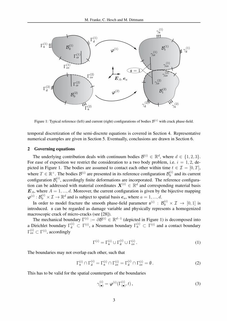
Figure 1: Typical reference (left) and current (right) configurations of bodies B(i) with crack phase-field.

temporal discretization of the semi-discrete equations is covered in Section 4. Representative

numerical examples are given in Section 5. Eventually, conclusions are drawn in Section 6.

2 Governing equations

The underlying contribution deals with continuum bodies B(i) ∈ Rd, where d ∈ {1, 2, 3}.

For ease of exposition we restrict the consideration to a two body problem, i.e. i = 1, 2, de-

picted in Figure 1. The bodies are assumed to contact each other within time t ∈ I = [0, T ],

where T ∈ R+. The bodies B(i) are presented in its reference configuration B

(i)0 and its current

configuration B(i)t , accordingly finite deformations are incorporated. The reference configura-

tion can be addressed with material coordinates X(i) ∈ Rd and corresponding material basis

EA, where A = 1, ..., d. Moreover, the current configuration is given by the bijective mapping

ϕ(i) : B(i)0 × I → R

d and is subject to spatial basis ea, where a = 1, ..., d.

In order to model fracture the smooth phase-field parameter s(i) : B

(i)0 × I → [0, 1] is

introduced. s can be regarded as damage variable and physically represents a homogenized

macroscopic crack of micro-cracks (see [28]).

The mechanical boundary Γ(i) := ∂B(i) ∈ Rd−1 (depicted in Figure 1) is decomposed into

a Dirichlet boundary Γ(i)d ⊂ Γ(i), a Neumann boundary Γ

(i)n ⊂ Γ(i) and a contact boundary

Γ(i)co ⊂ Γ(i), accordingly

Γ(i) = Γ(i)n ∪ Γ

(i)d ∪ Γ(i)

co . (1)

The boundaries may not overlap each other, such that

Γ(i)n ∩ Γ

(i)d = Γ(i)

n ∩ Γ(i)co = Γ

(i)d ∩ Γ(i)

co = ∅ . (2)

This has to be valid for the spatial counterparts of the boundaries

γ(i)(•) = ϕ(i)(Γ

(i)(•), t) , (3)

3


11

l l

X X

s(X)s(X)

Figure 2: 1D sharp (left) and phase-field regularized (right) crack.

as well, where the abbreviation (•) is used to refer to the different boundaries. In addition to

the mechanical boundaries a crack Dirichlet boundary Γ(i)cr defines a new internal boundary of

corresponding body and can be initialized within the bodies. All other phase-field boundaries

can be regarded as Neumann boundaries. For the two-field problem the displacement as well as

the scalar-valued phase-field parameter are the primary unknowns

[ϕ, s] ∈ Rd+1 . (4)

Phase-field contribution The aforementioned crack phase-field parameter s has two bounds,

the unbroken state with s = 0 and the fully broken state with s = 1 (see [28, 18]). Herein,

we assume that crack initiates or continues only in tensile state by attainment of a critical local

fracture energy density, given by G(i)c , which is related to the critical Griffith-type fracture en-

ergy (see [11, 21, 28]). The sharp crack is a d− 1-dimensional manifold. To avoid the difficult

modeling of sharp cracks we regularize the crack zone with a suitable crack density functional

γ(i)cr,n, such that we are able to integrate over the d-dimensional domain

G(i)c

∫

Γ(i)

dA ≈ G(i)c

∫

B(i)0

γ(i)cr,n dV = G(i)

c Γ(i)cr,n =: V (i)

cr,n .

Therein n denotes the order of the phase-field model (cf. [3]). In [28] a second order and

in [3, 34] a fourth order differential equation have been proposed1 (see Figure 3 for the 1D

analytical solution). The former is given by

s(i) − 4 (l(i))2 ∆s

(i) = 0 , (5)

with the corresponding functional

F(i)cr,2 =

1

2

∫

B(i)0

((s(i))2 + 4 (l(i))2 ∇s(i) · ∇s

(i)) dV , (6)

whereas the latter is given by

s(i) − 2 (l(i))2 ∆s

(i) + (l(i))4 ∆∆s(i) = 0 . (7)

The corresponding functional denotes

1It is important to remark, that it does not exist a natural PDE to model the crack density functional (for more

informations see [34])

4


Figure 3: Analytical solution of 1D second order phase-field (5) s(x) = e−|x|2 l (left) and fourth order phase-field

(7) s(x) = e−|x|

l (1 + |x|l) with different length scale parameters.

F(i)cr,4 =

1

2

∫

B(i)0

(1

2(s(i))2 + (l(i))2 ∇s

(i) · ∇s(i) +

(l(i))4

2∆s

(i) ∆s(i)) dV . (8)

In the above equations l(i) denotes the length scale parameter, which determines the width of

the regularization zone (see Figure 2). The length scale parameter may be treated as material

parameter and should be chosen as

h(i) <l(i)

2, (9)

where h(i) denotes the smallest finite element size (for more details see [28]). Note, for the

fourth order approach l(i) can be chosen even smaller as suggested by (9) (see e.g. [16]) The

regularized crack surface topologies are then constructed by Γ(i)cr,2/4 :=

1l(i)

F(i)cr,2/4 as proposed in

[28]. Accordingly, for (5) and (7), we obtain

Γ(i)cr,2 =

1

2 l(i)

∫

B(i)0

((s(i))2 + 4 (l(i))2 ∇s(i) · ∇s

(i)) dV , (10)

Γ(i)cr,4 =

1

4 l(i)

∫

B(i)0

((s(i))2 + 2 (l(i))2 ∇s(i) · ∇s

(i) + (l(i))4 ∆s(i)∆s

(i)) dV , (11)

respectively. As can be observed in Figure 3, the fourth order phase-field approach has two

advantages with respect to the second order phase-field approach. The fourth order phase-field

approach does not contain non-differentiable areas and further by using the same length scale

parameter the transition zone is smaller. Moreover, in the numerical treatment better accuracy

and convergence rates of the solution have been observed (see [3]). For the second order phase-

field model C0-continuity, whereas for the fourth order model C1-continuity is required.

Bulk contribution The potential of the bulk is given by

V(i)

bulk =

∫

B(i)0

Ψ(i) dV , (12)

5


where Ψ(i) denotes the strain energy density function of body i. The corresponding balance of

linear momentum is given by

Div(P (i)) + B(i)

= ρ(i)0 ϕ(i) , (13)

where P (i) : B(i)0 × I → R

d×d denotes the first Piola-Kirchhoff stress tensor, B(i)

∈ Rd

denotes the prescribed body force density and ρ(i)0 : B

(i)0 × I → R denotes the mass density.

Additionally, an arbitrary hyperelastic material law can be incorporated with a suitable strain

tensor. The symmetric right Cauchy-Green strain tensor is introduced by

C(i) = F (i) F (i)T , (14)

using the deformation gradient F (i) : B(i)0 × I → R

d×d. As already mentioned, we assume that

only local tension rather than local compression is responsible for crack growth. Accordingly,

we aim at an anisotropic description, such that we need to split the kinematic into tension and

compression2. Therefore we employ an eigendecomposition of the deformation gradient, which

yields

F (i) =d

∑

a=1

λ(i)a a(i)

a ⊗A(i)a , (15)

where the deformation gradient is represented in its principal stretches λ(i)a and spatial and mate-

rial directions a(i)a ,A(i)

a , respectively. As proposed by [18], an operator split of the deformation

gradient is performed, such that

F (i) = F (i),− F (i),+ =d

∑

a=1

λ(i),−a λ(i),+

a a(i)a ⊗A(i)

a . (16)

Therein the superscripted ± denotes

λ(i),±a =

λ(i)a ± |λ

(i)a |

2. (17)

Accordingly, the principal strains are decomposed into tensile and compressive components.

Furthermore, an anisotropic split of the principal stretches is accomplished, which yields

F (i) =: F(i)i

F (i)e

, (18)

where the fracture sensitive and insensitive parts are introduced as follows

F(i)i

=d

∑

a=1

(λ(i),+a )1−g(s(i)) aa ⊗Aa, F (i)

e=

d∑

a=1

(λ(i),+a )g(s

(i)) λ(i),−a aa ⊗Aa . (19)

Therein the degradation function g(s(i)) = 1− s(i) has been introduced. Note, in the linear case

an additive split has been proposed by [26] and can be stated as

Ψ(i)(ǫ(i)) → Ψ(i)(ǫi, s(i)) = (g(s(i)) + k)Ψ(i),+(ǫ(i)) + Ψi,−(ǫ(i)), g(s(i)) = (1− s(i))2 .

(20)

2Note, a less realistic but more simple choice would be an isotropic description.

6


EA, ea

B(1)t

B(2)t

γ(1)co

γ(2)co

γ(1)cr

γ(1)cr

γ(2)crγ

(2)cr

γ(1)n

γ(2)n

γ(1)d

γ(2)d

ϕ(1)

ϕ(2)n

ξ1ξ2

g

a1

a2

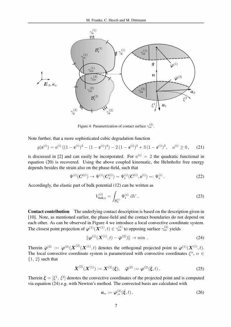
Figure 4: Parametrization of contact surface γ(2)co .

Note further, that a more sophisticated cubic degradation function

g(s(i)) = a(i) ((1− s(i))3 − (1− s

(i))2)− 2 (1− s(i))3 + 3 (1− s

(i))2, a(i) ≥ 0 , (21)

is discussed in [2] and can easily be incorporated. For a(i) = 2 the quadratic functional in

equation (20) is recovered. Using the above coupled kinematic, the Helmholtz free energy

depends besides the strain also on the phase-field, such that

Ψ(i)(C(i)) → Ψ(i)(C(i)e) = Ψ(i)

e(C(i), s(i)) =: Ψ(i)

e. (22)

Accordingly, the elastic part of bulk potential (12) can be written as

V(i)

bulk,e =

∫

B(i)0

Ψ(i)e

dV . (23)

Contact contribution The underlying contact description is based on the description given in

[10]. Note, as mentioned earlier, the phase-field and the contact boundaries do not depend on

each other. As can be observed in Figure 4 we introduce a local convective coordinate system.

The closest point projection of ϕ(1)(X(1), t) ∈ γ(1)co to opposing surface γ

(2)co yields

‖ϕ(1)(X(1), t)− ϕ(2))‖ → min . (24)

Therein ϕ(2) := ϕ(2)(X(2)(X(1), t) denotes the orthogonal projected point to ϕ(1)(X(1), t).

The local convective coordinate system is parametrized with convective coordinates ξα, α ∈{1, 2} such that

X(2)(X(1)) := X(2)(ξ), ϕ(2) := ϕ(2)(ξ, t) . (25)

Therein ξ = [ξ1, ξ2] denotes the convective coordinates of the projected point and is computed

via equation (24) e.g. with Newton’s method. The convected basis are calculated with

aα := ϕ(2),α (ξ, t) . (26)

7


Note that the above basis are in general not orthonormal. Accordingly, it is important to give

the metric for the local coordinate system

mαβ = aα · aβ . (27)

The gap vector is given by (see Figure 4)

g = ϕ(1) − ϕ(2) . (28)

Furthermore, the unit outward normal to the surface γ(2)co at point ϕ(2) is defined by

n :=a1 × a2

‖a1 × a2‖. (29)

With the above the scalar-valued gap function can be computed via

gN =(

ϕ(1) − ϕ(2))

· n . (30)

Considering the balance of linear momentum at the contact boundary, we obtain

t(1)co (X(1), t) dA(1) = −t(2)co (X

(2)(X(1)), t) dA(2) . (31)

Therein, the involved contact traction can be splitted into a normal and a tangential part as

follows

t(1)co (X(1), t) = tN + tT, tT · n = 0 . (32)

Moreover, the normal contact traction is given by

tN := t(1)N = −tN n . (33)

Frictionless contact is incorporated by using the well-known Karush-Kuhn-Tucker conditions,

given by

gN ≥ 0 , (34)

tN ≤ 0 , (35)

tN gN = 0 . (36)

The Karush-Kuhn-Tucker conditions are comprised of the impenetrability condition (34), the

condition which only allows compressive tractions (35) and the complementarity condition (36).

The Karush-Kuhn-Tucker conditions are shown in Figure 5 for both the penalty method and

Lagrange multipliers. Note, the framework is readily expendable to incorporate any frictional

constitutive law (e.g. Coulomb friction), but is omitted herein for convenience, i.e. tT = 0.

Within the computational treatment of contact, we subsequently apply the active set strategy to

obtain an active contact boundary Γ(i)co from the potential contact boundary Γ

(i)co . In particular

the inequalities given in (34)-(36) are implemented using the max-operator (see [20] for more

informations) as follows

ΦN = λN −max(0, λN − cΦN) = 0 . (37)

8


tN

gN

ǫN

admissible region

Figure 5: Karush-Kuhn-Tucker conditions for frictionless contact (solid line: exact enforcement, dotted line:

penalty regularization with penalty parameter ǫN).

Therein λN and ΦN denote the Lagrange multiplier and corresponding constraint, respectively.

Note λN := tN denotes the exact contact traction and ΦN := gN the gap function. Moreover,

within the active set strategy c ∈ R+ is a constant parameter, which is suitable to influence the

convergence of Newton’s method but does not influence the constraint enforcement. Eventually,

assuming active contact and using equation (31), we are able to introduce the contact potential

employing only one integral expression, such that

2∑

i=1

V (i)co =

∫

Γ(1)co

t(1)co ·(

ϕ(1) −ϕ(2))

dA(1) := Vco . (38)

Initial boundary value problem In the following the contact boundaries are assumed to be

known. Collecting all introduced contributions, yields

V aug =∑

i

V(i)

bulk,e + V(i)

cr,2/4 + Vco . (39)

Regarding transient problems the kinetic energy is defined by

T =∑

i

1

2

∫

B(i)0

ρ ϕ(i) · ϕ(i) dV . (40)

With the Lagrange functional L = T − V aug at hand, the above is used to employ Hamilton’s

principal, given by

δS =

∫ t2

t1

δL dt =

∫ t2

t1

(δT − δV aug) dt!= 0 . (41)

9


Equation (41) leads to the Euler-Lagrange equations. Accordingly, the initial boundary value

problem (IBVP), for the coupled system with fourth order phase-field model, can be written as

Div(F (i)e

S(i)e) + B

(i)− ρ

(i)0 ϕ(i) = 0 in B

(i)0 ∀t ∈ I , (42)

H(i) +G(i)c

4 l(i)(s(i) − 2 (l(i))2 ∆s

(i) + (l(i))4 ∆∆s(i)) = 0 in B

(i)0 ∀t ∈ I , (43)

ϕ(i) = ϕ(i) on Γ(i)d ∀t ∈ I , (44)

P (i) N (i) = T(i)

on Γ(i)n ∀t ∈ I , (45)

gN ≥ 0 on Γco∀t ∈ I , (46)

tN ≤ 0 on Γco∀t ∈ I , (47)

tN gN = 0 on Γco∀t ∈ I , (48)

s(i) = 1 on Γcr,d∀t ∈ I , (49)

∆s(i) = 0 on Γ(i)∀t ∈ I , (50)

∇((l(i))4 ∆s(i) − 2 (l(i))2 s(i)) ·N (i) = 0 on Γ(i)∀t ∈ I , (51)

ϕ(i)(t = 0) = ϕ(i)0 in B

(i)0 , (52)

ϕ(i)(t = 0) = ϕ(i)0 in B

(i)0 , (53)

s(i)(t = 0) = s

(i)0 in B

(i)0 . (54)

The above is supplemented by the constitutive equations

S(i)e

= 2 D1Ψ(i)e(C(i), s(i)), H(i) = D2Ψ

(i)e(C(i), s(i)) , (55)

which denote the second Piola-Kirchhoff stress tensor and the driving force of the phase-field.

Equations (44)-(45) are the prescribed mechanical Dirichlet and Neumann boundary conditions,

whereas equations (49)-(51) denote the phase-field Dirichlet and Neumann boundary condi-

tions. Furthermore equations (52)-(54) denote the initial conditions. Note, in order to obtain

the IBVP for the second order phase-field model, equation (43) needs to be exchanged by

H(i) +G(i)c

2 l(i)(s(i) − 4 (l(i))2 ∆s

(i)) = 0 in B(i)0 . (56)

Furthermore, equations (49) and (50) need to be exchanged by condition

∇s(i) = 0 on Γ(i)∀t ∈ I . (57)

Note that we do not enforce s ≥ 0. Accordingly, within our formulation, the phase-field may

be healed except the material is fully broken, i.e. s = 1, which will be enforced with a Dirichlet

type mechanism (see next paragraph for more informations).

Virtual work Analogously, we are able to collect the virtual work contributions, such that

G :=∑

i

G(i)dyn +G

(i)int,ext +G

(i)cr,2/4 + Gco . (58)

To this end the displacement solution space is defined by

V (i)s = {ϕ(i) : ϕ(i)(X(i), t) ∈ H1(B

(i)0 )|ϕ(i)(X(i), t) = ϕ(i) on Γ

(i)d } , (59)

10


such that the solution function ϕ(i) is element of the Sobolev space H1 which includes the space

of square-integrable functions and square-integrable first derivatives. Furthermore the solution

function is required to satisfy the Dirichlet boundary condition. The space of test functions with

the corresponding test function δϕ(i) is postulated as3

V(i)t = {δϕ(i) : δϕ(i)(X(i)) ∈ H1(B

(i)0 )|δϕ(i)(X(i)) = 0 on Γ

(i)d } . (60)

Accordingly, the test-function vanishes at the Dirichlet boundary. Using standard techniques,

the contributions to the weak form are obtained as follows

G(i)dyn :=

∫

B(i)0

δϕ(i) · ϕ(i) ρ(i)0 dV , (61)

G(i)int,ext :=

∫

B(i)0

S(i)e

: F (i)T

eGrad(δϕ(i)) dV −

∫

B(i)0

δϕ(i) · B(i)

dV −

∫

Γ(i)n

δϕ(i) · T(i)

dV .

(62)

Using a suitable test space for the second order PDE in (5), e.g. given by

Vs,(i)cr,2 = {s(i) : s(i)(X(i), t) ∈ H1(B

(i)0 )|s(i) = 1 on Γ(i)

cr } , (63)

Vt,(i)cr,2 = {δs(i) : δs(i)(X(i)) ∈ H1(B

(i)0 )|δs(i) = 0 on Γ(i)

cr } , (64)

where Γ(i)cr denotes a sharp crack inside B

(i)0 and thus can be regarded as Dirichlet condition,

yields the weak form

G(i)cr,2 :=

G(i)c

2 l(i)

∫

B(i)0

(

δs(i) (s(i) +2 l(i)

G(i)c

H(i)) + 4 (l(i))2 Grad(δs(i)) ·Grad(s(i))

)

dV . (65)

For the fourth order PDE given in (7), a test space which provides higher continuity is needed,

such as

Vs,(i)cr,4 = {s(i) : s(i)(X(i), t) ∈ H2(B

(i)0 )|s(i) = 1 on Γ(i)

cr } , (66)

V t,(i)cr,4 = {δs(i) : δs(i)(X(i)) ∈ H2(B(i)

0 )|δs(i) = 0 on Γ(i)cr } . (67)

Accordingly, the weak form is obtained by

G(i)cr,4 :=

G(i)c

4 l(i)

∫

B(i)0

(δs(i) (s(i) +4 l(i)

G(i)c

H(i)) + 2 (l(i))2 Grad(δs(i)) ·Grad(s(i))

+ (l(i))4 ∆δs(i) ·∆s(i)) dV . (68)

Using Lagrange multipliers for the incorporation of the contact conditions, the virtual work of

contact yields

Gco = GλNco + Gϕ

co , (69)

3Note that the test function δϕ(i) can also be interpreted as virtual displacement.

11


where GλNco := δλN

Vco and Gϕco := δϕVco have been introduced. Eventually, the governing

equations are obtained as follows4

∑

i

G(i)dyn +G

(i)int,ext + Gϕ

co = 0, ∀δϕ(i) ∈ V(i)t , (70)

∑

i

G(i)cr,2/4 = 0, ∀δs(i) ∈ V

(i)cr,2/4 , (71)

GλNco = 0, ∀δλN ∈ R . (72)

Note, the abbreviation 2/4 indicates that either the virtual work of the second order phase-field

equation (65) or the virtual work of the fourth order phase-field equation (68) can be taken into

account.

3 Spatial discretization

To perform the spatial discretization for the numerical solution of the variational formulation

each domain is subdivided into a finite set of non-overlapping elements

B(i) ≈ B(i),h =

n(i)el⋃

e

B(i),h,e . (73)

For the second order phase-field model standard FEA with C0 continuous shape functions is

sufficient, whereas for the fourth order phase-field model we need to apply C1 continuous shape

functions which we accomplish using IGA.

Standard FEA – Allen-Cahn phase-field model For the second order phase-field model

we are able to use standard Lagrangian shape functions and isoparametric as well as Bubnov-

Galerkin FE interpolations. Accordingly, solution and test functions are approximated by

ϕ(i),h = LA q(i)A , δϕ(i),h = LA δq

(i)A , X(i),h = LA X

(i)A , (74)

s(i),h = LA s

(i)A , δs(i),h = LA δs

(i)A , ∀A ∈ ω = {1, . . . , nnode} . (75)

Here L(i)A (X(i)) : B0 → R denote Lagrangian shape functions. Inserting these approximations

into the weak forms given in (70)–(72) yields the semi-discrete virtual work∑

i

δq(i)A · (M

(i)ABq

(i)B + F

(i),int

A − F(i),ext

A ) + Gϕ,hco = 0 , (76)

∑

i

δs(i)A

∫

B(i)0

(L(i)A H(i),h +

G(i)c

l(i)L(i)A L

(i)B s

(i)B + 4G(i)

c l(i)∇L(i)A · ∇L

(i)B s

(i)B ) dV = 0 , (77)

GλN,hco = 0 . (78)

Here, M(i)AB =

∫

B0ρ0L

(i)A L

(i)B dV are the coefficients of the consistent mass matrix. Further-

more, F(i),intA , F

(i),extA denote the nodal internal and external force vectors. Note the semi-

discrete contact contributions Gϕ,hco and GλN,h

co are dealt with in the very last paragraph of this

section.

4Strictly speaking, the underlying virtual work (38) is not an equality but an inequality equation, due to the

contact constraints (34)-(36) involved. As already mentioned, here and in what follows it is assumed that the

contact interface is known using e.g. an active set strategy, regularization techniques or others. Based on this

assumption the virtual work can be written as an equality (see e.g. [37, 35]).

12


0 1 2 3 4

0

1

C−1 C−1C2 C1 C0

Figure 6: Continuity of cubic B-splines with knot vector Θ = [0 0 0 0 1 2 2 3 3 3 4 4 4 4].

IGA – Cahn-Hilliard phase-field model For the higher order Cahn-Hilliard phase-field model

we use an IGA approach to satisfy the demand for C1 continuity. For the approximation we use

a linear combination of suitable splines and corresponding solution and test control variables

ϕ(i),h = R(i)A q

(i)A , δϕ(i),h = R

(i)A δq

(i)A , s

(i),h = R(i)A s

(i)A , δs(i),h = R

(i)A δs

(i)A ,

∀A ∈ ω = {1, . . . , nnode} . (79)

Here R(i)A (X(i)) : B0 → R denote multivariate NURBS with tensor product structure

R(i)A = R(i),i

p (ξ(i)) =Πd

l=1N(i)il,pl

(ξ(i),l)w(i)il

∑

i Πdl=1N

(i)

il,pl(ξ(i),l)w

(i)

il

, (80)

Therein i = [i1, ..., id] denote the multi index of the B-splines N(i)il,pl

with multi index p =[p1, ..., pd] for the respective order of each parametric direction. Moreover, wi denote the

NURBS weights. A comprehensive overview for IGA can be found in [6]. Note, for global

C1-continuity, which is required for the Cahn-Hilliard phase-field model, at least quadratic B-

splines need to be provided. B-splines are recursively defined. For order pl = 0 we have

N(i)il,pl=0(ξ

(i),l) =

{

1 if ξ(i),lil

≤ ξ(i),l < ξ(i),lil+1

0 otherwise, (81)

whereas for order pl > 0 the corresponding B-spline can be computed with

N(i)il,pl

(ξ(i),l) =ξ(i),l − ξ

(i),lil

ξ(i),lil+pl

− ξ(i),lil

N(i)il,p−1(ξ

(i),l) +ξ(i),lil+pl+1 − ξ(i),l

ξ(i),lil+pl+1 − ξ

(i),lil+1

N(i)il+1,p−1(ξ

(i),l) , (82)

where problem specific knot vectors need to be provided

Θ(i),l = [ξ(i),l1 , . . . , ξ

(i),lnl+pl+1] . (83)

13


Figure 7: Hierarchical level 1 subdivision of 1D linear, cubic and quintic B-splines (black: original spline/parent,

colored: ’refined’ splines/children).

With the knot vectors both the finite element mesh as well as the continuity is determined (see

Figure 6). B-splines and NURBS basis functions are local linear independent

∑

A

cAR(i)A (ξ(i)) = 0 ⇔ cA = 0 . (84)

Furthermore the partition of unity is fulfilled

∑

A

R(i)A (ξ(i)) = 1 . (85)

Another property is that B-splines as well as NURBS only have minimal support. In general

B-splines and NURBS are non-interpolatory but can be constructed that they are. B-splines and

NURBS basis functions are always positive, i.e.

R(i)A (ξ(i)) > 0 . (86)

As refinement techniques h-refinement e.g. achieved via knot insertion leads to expensive global

refinement. For local refinement techniques there mainly exists T-splines, which are the IGA

representation of hanging nodes and the concept of hierarchical refinement which we want to

apply subsequently. For hierarchical B-splines the basis functions are subdivided instead of

the elements. In particular the B-spline to be refined (parent) is replaced by using a linear

combination of copied and scaled version of the original B-spline (children) via

B(i),A = B(i),ip (ξ(i)) =

p+1∑

j=0

d∏

l=1

2−pl

(

pl + 1

jl

)

N(i)il,pl

(2ξ(i),l − j(i)l h

(i)l − ξ

(i),lil

) . (87)

Therein hl refers to the coarse level element length in the parameter space. The refinement

procedure for one level is shown for the one-dimensional case in Figure 7 and for the two-

dimensional case in Figure 8. Next we rewrite the hierarchical B-splines given in equation (87)

approach by using the subdivision matrix S(i), S(i)i,j which contains the scaling. A single B-

spline on level k can then be replaced by its children, which correspond to B-splines on level

k + 1

B(i),i,kp (ξ(i)) =

p+1∑

j=0

S(i)i,jB

(i),2i−1+j,k+1p (ξ(i)) . (88)

14


Figure 8: Subdivision of a 2D quartic B-spline (left: parent, right: children).

This is only valid for uniform knot vectors (for non-uniform knot vectors, see Sabin [32]).

Afterwards, the control mesh needs to be extended by

q(i),k+1A = S

(i),T

A q(i),kA , s

(i),k+1A = S

(i),T

A s(i),kA , (89)

where q(i),k+1A represents a set of new coordinates. The extension of B-splines to NURBS is

given by

R(i),kA = R(i),i,k

p (ξ(i)) =

p+1∑

j=0

S(i)i,jB

(i),2i−1+j,k+1p (ξ(i))w

(i),k+12i−1+j

∑

i

p+1∑

j=0

Si,jB(i),2i−1+j,k+1p (ξ(i))w

(i),k+12i−1+j

. (90)

The partition of unity as well as the continuity are still satisfied. For further details see [29].

Insertion of the polynomial approximations into the virtual work of the coupled phase-field

system yields

∑

i

δq(i)A · (M

(i)ABq

(i)B + F

(i),int

A − F(i),ext

A ) +Gϕ,hco = 0 , (91)

∑

i

δs(i)A

∫

B(i)0

(R(i)A H(i),h +

G(i)c

l(i)R

(i)A R

(i)B s

(i)B + 4G(i)

c l(i)∇R(i)A · ∇R

(i)B s

(i)B ) dV = 0 , (92)

GλN,hco = 0 . (93)

Here, M(i)AB =

∫

B0ρ0R

(i)A R

(i)B dV are the coefficients of the consistent mass matrix. Further-

more, F(i),int

A , F(i),ext

A denote the nodal internal and external force vectors, approximated with

HNURBS. As constitutive relations the discrete second Piola-Kirchhoff stress tensor as well as

the driving force for the phase-field

S(i),he

= 2 D1Ψ(i)e(C(i),h, s(i),h), H(i),h = D2Ψ

(i)e(C(i),h, s(i),h) , (94)

need to be provided.

15


Mortar contact element For the discretization of the contact interface we aim at a Mortar

approach. Herein, we restrict our consideration to the IGA case for the Lagrange discretized

case we refer to the Mortar method given in [15]. In order to simplify the approach without

violation of the required C1 continuity of the primal space we use linear approximation of the

dual space as has been proposed in [17, 7]. Accordingly, the contact traction is approximated

as follows

t(1),hco =∑

A∈ω(1)

LAλA, δt(1),hco =∑

A∈ω(1)

LAδλA . (95)

Therein ω(1) = [q1, . . . , qnsurf] denotes nsurf nodes on the physical contact boundary γ

(1)co . More-

over, LA : Γ(1)co → R are (d − 1)-dimensional shape functions associated with nodes A ∈ ω(1).

It is important to remark, that the discrete Lagrange multiplier space for refined contact regions

can provide possible singularities (for more informations see [16]). Eventually, we are able to

state the semi-discrete contact contribution

Gϕ,hco = λN,An ·

[

nABδq(1)B − nACδq

(2)C

]

+ λN,Aδn ·[

nABq(1)B − nACq

(2)C

]

. (96)

Therein the nodal normal traction λN,A is employed. Furthermore, the Mortar integrals

nAB =

∫

Γ(1),hco

LA(ξ(1))RB(ξ

(1)) dA, (97)

nAC =

∫

Γ(1),hco

LA(ξ(1))RC(ξ

(2)) dA , (98)

are comprised of the above introduced linear shape functions LA(ξ(1)) for the dual and quadratic

shape functions RB(ξ(1)), RC(ξ

(2)) for the primal space. In order to be able to integrate the

contact contributions we provide an isoparametric transformation

ξ(i),h(η) =3

∑

K=1

MK(η)ξ(i)K , (99)

where we make use of bilinear, triangular shape functions MK . The segment-wise Mortar

integrals are then given by

nκβ =

∫

△

Lκ(ξ(1),h(η))Rβ(ξ

(1),h(η))Jseg dη , (100)

nκζ =

∫

△

Lκ(ξ(1),h(η))Rζ(ξ

(2),h(η))Jseg dη . (101)

Therein Jseg denotes the segment-wise Jacobian. Using the tangential vectors in the reference

configuration Aα(ξ) = RA,α(ξ)qA the segment-wise Jacobian can be computed by

Jseg = ‖A1(ξ(1),h(η))×A2(ξ

(1),h(η))‖det(Dξ(η)) . (102)

Eventually the segment-wise contact contributions needs to be assembled into the global system.

For a more detailed explanation of the Mortar method, especially the technically demanding

segmentation and the assembly see [14, 15, 17, 7].

16


4 Temporal discretization

For the temporal discretization we subdivide the time interval I of interest into N equidistant

increments ∆t = tn+1 − tn, as follows

I = [0, T ] =N−1⋃

n=0

[tn, tn+1] , (103)

where in the following the variables qnA, snA at time tn are assumed to be known, whereas the

variables qn+1A , sn+1

A at time tn+1 are searched. Then we employ a second order accurate one

step midpoint-type discretization. In particular the fully discrete equations

∑

i

δq(i)A · (M

(i)AB

q(i),n+1B − q

(i),nB

∆t+

∫

B(i)0

∇R(i)A (X(i)) · S(i),n,n+1

e∇R

(i)B (X(i)) dV q

(i),n+ 12

B

−

∫

B(i)0

F(i),ext,n+ 1

2

A dV ) +Gϕ,n,n+1co = 0 , (104)

∑

i

δs(i)A

∫

B(i)0

R(i)A H(i),n+ 1

2 +Gc

2lR

(i)A R

(i)B s

(i),n+ 12

B + Gc l∇R(i)A · ∇R

(i)B s

(i),n+ 12

B

+Gc l

3

2∆R

(i)A ∆R

(i)B s

(i),n+ 12

B dV = 0 , (105)

GλN,n,n+1co = 0 , (106)

are obtained. In order to obtain a structure preserving time integration scheme, an algorithmic

stress computation

S(i),n,n+1e

=2∂Ψ(i),n+ 1

2

∂C(i),h

+ 2Ψ

(i),n+1e −Ψ

(i),ne + G

(i)c (γ(i),n+1 − γ(i),n)− ∂Ψ

(i),n+12

e

∂C(i),h : ∆C(i),h

∆C(i),h : ∆C(i),h∆C(i),h , (107)

using the concept of the discrete gradient is employed. Note that the concept of the discrete

gradient exhibits superior stability and robustness properties even for large time steps. The

fully discrete contact contributions can be calculated by

Gϕ,n,n+1co = λ

n,n+1A nn+ 1

2 ·[

nnABδq

(1)B − nn

ACδq(2)C

]

+ δλAδnn+ 1

2 ·[

nnABq

(1)B − nn

ACq(2)C

]

,

GλN,n,n+1co = δλAn

n+ 12 ·

[

nnAB q

(1)B − nn

AC q(2)C

]

.

5 Numerical examples

In order to show the enhanced properties of the proposed methods two representative numeri-

cal examples are examined. In particular the proposed hierarchical NURBS based discretization

with the Mortar contact method and the phase-field approach to fracture are investigated in the

examples, where local refinements are predefined. Note, for the simple geometries employed,

all NURBS weights are chosen equal to one, such that the NURBS can be considered as B-

splines.

17


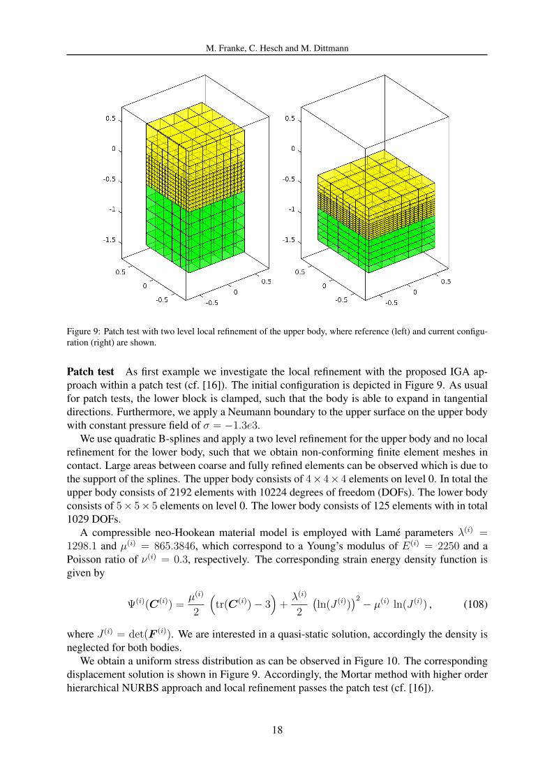
Figure 9: Patch test with two level local refinement of the upper body, where reference (left) and current configu-

ration (right) are shown.

Patch test As first example we investigate the local refinement with the proposed IGA ap-

proach within a patch test (cf. [16]). The initial configuration is depicted in Figure 9. As usual

for patch tests, the lower block is clamped, such that the body is able to expand in tangential

directions. Furthermore, we apply a Neumann boundary to the upper surface on the upper body

with constant pressure field of σ = −1.3e3.

We use quadratic B-splines and apply a two level refinement for the upper body and no local

refinement for the lower body, such that we obtain non-conforming finite element meshes in

contact. Large areas between coarse and fully refined elements can be observed which is due to

the support of the splines. The upper body consists of 4× 4× 4 elements on level 0. In total the

upper body consists of 2192 elements with 10224 degrees of freedom (DOFs). The lower body

consists of 5× 5× 5 elements on level 0. The lower body consists of 125 elements with in total

1029 DOFs.

A compressible neo-Hookean material model is employed with Lame parameters λ(i) =1298.1 and µ(i) = 865.3846, which correspond to a Young’s modulus of E(i) = 2250 and a

Poisson ratio of ν(i) = 0.3, respectively. The corresponding strain energy density function is

given by

Ψ(i)(C(i)) =µ(i)

2

(

tr(C(i))− 3)

+λ(i)

2

(

ln(J (i)))2

− µ(i) ln(J (i)) , (108)

where J (i) = det(F (i)). We are interested in a quasi-static solution, accordingly the density is

neglected for both bodies.

We obtain a uniform stress distribution as can be observed in Figure 10. The corresponding

displacement solution is shown in Figure 9. Accordingly, the Mortar method with higher order

hierarchical NURBS approach and local refinement passes the patch test (cf. [16]).

18


Figure 10: Von Mises stress distribution.

Bending contact fracture problem The next example deals with the contact of an elastic

block with an elastic plate. Note, this example is taken from [16]. The initial configuration is

depicted in Figure 11. As can be observed, the plate is clamped whereas the upper boundary of

the block is moved downwards with a constant increment size of ∆u = 5e-3 e3 for the first 200

steps and ∆u = 2.5× 10−3 e3 for the remaining steps.

The plate is of size 20 × 30 × 2 , whereas the block is of size 4 × 4 × 4. The center point

of the plate is placed at[

0 15 1]

and the center point of the block is placed at[

0 26 4.5]

.

The block consists of 4 × 4 × 4 elements and the plate of 13 × 19 × 2 elements on level 0.

Additionally, we apply a predefined local hierarchical refinement to account for the physical

events (contact and fracture). Therefore the contact zone of the block is locally refined with one

level. The plate is locally refined using one level refinement in the area of the expected contact

boundary and two level refined at the clamping zone (see Figure 11). In total 12948 elements

with overall 72912 DOFs and minimal element size of hmin = 0.0769 are employed.

Both bodies are modeled using the compressible neo-Hookean material model given in (108).

The Lame parameters of the plate are chosen as λ(1) = 1.1538e7 and µ(1) = 7.6923e6, which

Figure 11: Reference configuration of bending contact fracture problem.

19


Figure 12: Final phase-field (left) and σ22 stress (right) result of bending contact fracture problem.

correspond to a Young’s modulus of E(1) = 2e7 and a Poisson ratio of ν(1) = 0.3. The Lame

parameters of the block are chosen as λ(2) = 2.8846e4 and µ(2) = 1.9231e4, which correspond

to a Young’s modulus of E(2) = 5e4 and a Poisson ratio of ν(2) = 0.3. Accordingly, we expect

no locking behavior and there is no need for an advanced finite element model. For the plate

the phase-field parameters are chosen as Gc = 2.7 · e2 and l = 0.1538.

The final phase-field result as well as the final σ22 stress distribution are depicted in Figure

12. As can be observed the plate ripped out of the clamping zone, such that the plate becomes

statically undetermined. Accordingly, the problem can not be solved anymore with the consid-

ered quasi-static setup. Note, a more detailed explanation and examination of this example is

given in [16].

6 CONCLUSIONS

The underlying contribution introduces a large deformation framework to describe both con-

tact and fracture. For the former the variational consistent Mortar method, whereas for the latter

the phase-field method is used. In particular an accurate and smooth fourth order phase-field

model is employed which requires global C1 continuity. Therefore an existing IGA framework

with a sophisticated Mortar method for the contact boundaries is combined. With the proposed

NURBS-IGA approach a wide range of curved geometries can be approximated exactly. More-

over, an hierarchical refinement scheme is employed which does not violate the partition of

unity. This allows the local refinement of the bodies in order to account for different physical

events like e.g. contact or fracture.

In total an accurate and efficient higher order method is proposed for computational modeling

of large deformation Mortar contact and phase-field fracture problems.

REFERENCES

[1] A.-V. Vuong and C. Giannelli and B. Juttler and B. Simeon. A hierarchical approach to

adaptive local refinement in isogeometric analysis. Comput. Methods Appl. Mech. Engrg.,

200:3554–3567, 2011.

[2] M.J. Borden. Isogeometric Analysis of Phase-Field Models for Dynamic Brittle and Duc-

tile Fracture. PhD thesis, The University of Texas at Austin, 2012.

[3] M.J. Borden, T.J.R. Hughes, C.M. Landis, and C.V. Verhoosel. A higher-order phase-

field model for brittle fracture: Formulation and analysis within the isogeometric analysis

framework. Comput. Methods Appl. Mech. Engrg., 273:100–118, 2014.

20


[4] P.B. Bornemann and F. Cirak. A subdivision-based implementation of the hierarchical b-

spline finite element method. Comput. Methods Appl. Mech. Engrg., 253:584–598, 2013.

[5] B. Bourdin, G.A. Francfort, and J.J. Marigo. The variational approach to fracture. Journal

of Elasticity, 9:5–148, 2008.

[6] J.A. Cottrell, T.J.R. Hughes, and Y. Bazilevs. Isogeometric Analysis: Toward Integration

of CAD and FEA. Wiley, New York, 2009.

[7] M. Dittmann, M. Franke, I. Temizer, and C. Hesch. Isogeometric Analysis and thermome-

chanical Mortar contact problems. Comput. Methods Appl. Mech. Engrg., 274:192–212,

2014.

[8] D. Forsey and R.H. Bartels. Hierarchical B-Spline refinement. Comput. Graph., 22:205–

212, 1988.

[9] G.A. Francfort and J.-J. Marigo. Revisiting brittle fracture as an energy minimization

problem. Journal of the Mechanics and Physics of Solids, 46:1319–1342, 1998.

[10] M. Franke. Discretisation techniques for large deformation computational contact elasto-

dynamics. PhD thesis, Karlsruhe Institute of Technology, 2014.

[11] A.A. Griffith. The phenomena of rupture and flow in solids. Philosophical Transactions

of the Royal Society London, 221:163–198, 1921.

[12] H. Henry. Study of the branching instability using a phase field model of inplane crack

propagation. EPL, 83:16004, 2008.

[13] H. Henry and H. Levine. Dynamic instabilities of fracture under biaxial strain using a

phase field model. Physics Review Letters, 93:105505, 2004.

[14] C. Hesch and P. Betsch. Transient 3D Domain Decomposition Problems: Frame-

indifferent mortar constraints and conserving integration. Int. J. Numer. Methods Eng.,

82:329–358, 2010.

[15] C. Hesch and P. Betsch. Transient three-dimensional contact problems: mortar method.

Mixed methods and conserving integration. Computational Mechanics, 48:461–475,

2011.

[16] C. Hesch, M. Franke, M. Dittmann, and I. Temizer. Hierarchical NURBS and a higher-

order phase-field approach to fracture for finite-deformation contact problems. Computer

Methods in Applied Mechanics and Engineering, 301:242–258, 2016.

[17] C. Hesch and P.Betsch. Isogeometric analysis and domain decomposition methods. Com-

put. Methods Appl. Mech. Engrg., 213:104–112, 2012.

[18] C. Hesch and K. Weinberg. Thermodynamically consistent algorithms for a finite-

deformation phase-field approach to fracture. Int. J. Numer. Meth. Engng., 99:906–924,

2014.

[19] Schuß S. Dittmann M. Franke M. Hesch, C. and K. Weinberg. Isogeometric analysis

and hierarchical refinement for higher-order phase-field models. Computer Methods in

Applied Mechanics and Engineering, 303:185–207, 2016.

21


[20] M. Hintermueller, K. Ito, and K. Kunisch. The primal-dual active set strategy as a semis-

mooth Newton method. SIAM J. Optim., 13:865–888, 2003.

[21] G.R. Irwin. Elasticity and plasticity: fracture. In S. Fugge, editor, Encyclopedia of Physics,

1958.

[22] W. Jiang and J.E. Dolbow. Adaptive refinement of hierarchical B-spline finite elements

with an efficient data transfer algorithm. Int. J. Numer. Meth. Engng., 2014.

[23] A. Karma, D.A. Kessler, and H. Levine. Phase-field model of mode III dynamic fracture.

Physical Review Letter, 81:045501, 2001.

[24] C. Kuhn and R. Muller. A continuum phase field model for fracture. Engineering Fracture

Mechanics, 77:3625–3634, 2010.

[25] T.A. Laursen. Computational Contact and Impact Mechanics. Springer-Verlag, 2002.

[26] C. Miehe, M. Hofacker, and F. Welschinger. A phase field model for rate-independent

crack propagation: Robust algorithmic implementation based on operator splits. Comput.

Methods Appl. Mech. Engrg., 199:2765–2778, 2010.

[27] C. Miehe and L.M. Schanzel. Phase field modeling of fracture in rubbery polymers. Part

I: Finite elasticity coupled with brittle failure. Journal of the Mechanics and Physics of

Solids, page in press, 2013.

[28] C. Miehe, F. Welschinger, and M. Hofacker. Thermodynamically consistent phase-field

models of fracture: Variational principles and multi-field FE implementations. Int. J.

Numer. Meth. Engng., 83:1273–1311, 2010.

[29] R. Ortigosa, A.J. Gil, J. Bonet, and C. Hesch. A computational framework for polyconvex

large strain elasticity for geometrically exact beam theory. Computational mechanics,

2015, DOI:10.1007/s00466-015-1231-5.

[30] A. Popp, M. Gitterle, W. Gee, and W.A. Wall. A dual mortar approach for 3D finite

deformation contact with consistent linearization. Int. J. Numer. Methods Eng., 83:1428–

1465, 2010.

[31] M.A. Puso. A 3D mortar method for solid mechanics. Int. J. Numer. Methods Eng.,

59:315–336, 2004.

[32] M. Sabin, editor. Analysis and Design of Univariate Subdivision Schemes. Springer,

Heidelberg, 2010.

[33] D. Schillinger, L. Dede, M.A. Scott, J.A. Evans, M.J. Borden, E. Rank, and T.J.R. Hughes.

An isogeometric design–through–analysis methodology based on adaptive hierarchical re-

finement of NURBS, immersed boundary methods, and T–spline CAD surfaces. Comput.

Methods Appl. Mech. Engrg., 249–252:116–150, 2012.

[34] K. Weinberg and C. Hesch. A high-order finite-deformation phase-field approach to frac-

ture. Continuum Mechanics and Thermodynamics, pages 1–11, 2015.

[35] K. Willner. Kontinuums- und Kontaktmechanik. Springer-Verlag, 2003.

22


[36] B.I. Wohlmuth. Variationally consistent discretization schemes and numerical algorithms

for contact problems. Acta Numerica, 20:569–734, 2011.

[37] P. Wriggers. Computational Contact Mechanics. Springer-Verlag, 2nd edition, 2006.

23

Documents

A HIGHER ORDER PHASE-FIELD APPROACH TO FRACTURE FOR FINITE … · VII European Congress on Computational Methods in Applied Sciences and Engineering M. Papadrakakis, V. Papadopoulos,