Applied Mathematics and Computation 244 (2014) 606–612

Contents lists available at ScienceDirect

Applied Mathematics and Computation

journal homepage: www.elsevier .com/ locate /amc

A hybrid FEM for solving the Allen–Cahn equation

http://dx.doi.org/10.1016/j.amc.2014.07.0400096-3003/� 2014 Elsevier Inc. All rights reserved.

⇑ Corresponding author.E-mail address: cfdkim@korea.ac.kr (J. Kim).URL: http://math.korea.ac.kr/~cfdkim (J. Kim).

Jaemin Shin a, Seong-Kwan Park b, Junseok Kim c,⇑a Institute of Mathematical Sciences, Ewha W. University, Seoul 120-750, Republic of Koreab Department of Mathematics, Yonsei University, Seoul 120-749, Republic of Koreac Department of Mathematics, Korea University, Seoul 136-713, Republic of Korea

a r t i c l e i n f o a b s t r a c t

Keywords:Allen–Cahn equationFinite element methodOperator splitting methodUnconditionally stable scheme

We present an unconditionally stable hybrid finite element method for solving the Allen–Cahn equation, which describes the temporal evolution of a non-conserved phase-fieldduring the antiphase domain coarsening in a binary mixture. Its various modified formshave been applied to image analysis, motion by mean curvature, crystal growth, topologyoptimization, and two-phase fluid flows. The hybrid method is based on the operator split-ting method. The equation is split into a heat equation and a nonlinear equation. An impli-cit finite element method is applied to solve the diffusion equation and then the nonlinearequation is solved analytically. Various numerical experiments are presented to confirmthe accuracy and efficiency of the method. Our simulation results are consistent with pre-vious theoretical and numerical results.

� 2014 Elsevier Inc. All rights reserved.

1. Introduction

To model antiphase domain coarsening in a binary alloy, the following Allen–Cahn (AC) equation was introduced [1]:

@/ðx; tÞ@t

¼ � F 0ð/ðx; tÞÞ�2 þ D/ðx; tÞ; x 2 X; t > 0; ð1Þ

where X � R2 is a domain. The quantity /ðx; tÞ is defined as the difference of concentrations / ¼ cA � cB, where cA and cB arethe mass fractions of components A and B in a binary mixture. The function Fð/Þ ¼ 0:25ð/2 � 1Þ2 is the Helmholtz free energydensity. The small positive constant � is the gradient energy coefficient related to the interfacial energy. The system is com-pleted by taking initial and natural boundary conditions n � r/ ¼ 0, where n is normal to @X. The AC equation is a gradientflow with the Ginzburg–Landau free energy

Eð/Þ :¼Z

X

Fð/Þ�2 þ

jr/j2

2

!dx:

To show the total energy Eð/Þ is non-increasing in time, we differentiate the energy Eð/Þ with respect to time t

dEð/Þdt

¼Z

X

F 0ð/Þ�2 /t þr/ � r/t

� �dx ¼

ZX

F 0ð/Þ�2 � D/

� �/tdxþ

Z@X

n � r/ð Þ/tds ¼ �Z

X/2

t dx 6 0;

J. Shin et al. / Applied Mathematics and Computation 244 (2014) 606–612 607

where we have used the homogeneous Neumann boundary condition. The AC equation has been solved by using variousnumerical approaches such as the finite element, finite difference, and Fourier-spectral methods [2–7]. The various modifiedforms of AC equation have been applied to image analysis [8–10], motion by mean curvature [11–14], crystal growth [15,16],topology optimization [17,18], and two-phase fluid flows [19,20]. In general, finite element method (FEM) is better thanfinite difference method (FDM) in dealing with complicated domain problems. In FDM framework, a hybrid scheme was usedin [3]. However, it is not used in FEM. Therefore, the objective of this paper is to develop an unconditionally stable hybridfinite element method for solving the Allen–Cahn equation.

This paper is organized as follows. In Section 2, we describe the numerical solution algorithm of the AC equation. Thenumerical results showing the robustness and superiority of the proposed scheme are presented in Section 3. In Section 4,conclusions are drawn.

2. Numerical solution

We present an unconditionally stable hybrid scheme for solving the AC equation using the finite element method. LetH1ðXÞ denote the trial solution space. We partition X into a set T h consisting of a triangular element s. Let

Vh ¼ fw 2 Cð�XÞ : wjs is linear 8s 2 T hg � H1ðXÞ be the finite element space. Let fxigNi¼1 be the nodes of T h and let fgig

Ni¼1

be the linear basis functions such that gi 2 Vh;giðxjÞ ¼ dij, for i, j ¼ 1; � � � ;N, where N is the dimension of the discrete space.

We denote /i as the approximation of /ðxiÞ and define as /h ¼PN

i¼1/igi. We formally split the AC equation (1) into the heatand nonlinear differential equations as follows:

@/ðx; tÞ@t

¼ D/ðx; tÞ; ð2Þ

@/ðx; tÞ@t

¼ � F 0ð/ðx; tÞÞ�2 : ð3Þ

We numerically solve Eq. (2) by using a fully implicit finite element method and analytically solve Eq. (3) by using themethod of separation of variables. First, given /n

h, the finite element approximation to Eq. (2) is to find /�h such that forall wh 2 Vh

/�h � /nh

Dt;wh

� �þ ðr/�h;rwhÞ ¼ 0; ð4Þ

where Dt is the time step and ð�; �Þ is the inner product. Eq. (4) leads to the standard Galerkin method ðM þ dtKÞ/�h ¼ M/nh ,

where M ¼ ðmijÞ and K ¼ ðkijÞ are the mass and stiffness matrices with elements mij ¼ ðgi;gjÞ and kij ¼ ðrgi;rgjÞ. Becausethe standard Galerkin method does not guarantee the maximal principle [22], we use the lumped mass method

ðM þ dtKÞ/�h ¼ M/nh , where M obtained by taking for its diagonal elements �mii ¼

PNj¼1mij. For the implementation, we refer

to [21]. Second, by the method of separation of variables, Eq. (3) is solved analytically with the initial condition /�h.

/nþ1h ¼ /�hffiffiffiffiffiffiffiffiffiffiffiffiffiffiffiffiffiffiffiffiffiffiffiffiffiffiffiffiffiffiffiffiffiffiffiffiffiffiffiffiffiffiffiffiffiffiffiffiffiffi

��2Dt�2 þ /�h

� �2 1� e�2Dt�2

� �r : ð5Þ

In summary, to calculate /nþ1h from /n

h , we solve Eqs. (4) and (5).The stability of the proposed numerical scheme should be studied to get a reasonable solution. We prove that the pro-

posed scheme is unconditionally stable. Assume that k/nk1 6 1. The stability analysis [22] shows that the lumped massmethod of Eq. (4) is unconditionally stable. In addition, the inequality j/�j 6 k/nk1 is satisfied by the maximal principlefor the heat equation, and it implies that k/�k1 6 1. And, for the Eq. (5), we have the inequality

j/nþ1i j ¼ j/�i jffiffiffiffiffiffiffiffiffiffiffiffiffiffiffiffiffiffiffiffiffiffiffiffiffiffiffiffiffiffiffiffiffiffiffiffiffiffiffiffiffiffiffiffiffiffiffiffiffi

e�2Dt�2 þ ð/�i Þ

2 1� e�2Dt�2

� �r ¼ 1ffiffiffiffiffiffiffiffiffiffiffiffiffiffiffiffiffiffiffiffiffiffiffiffiffiffiffiffiffiffiffiffiffiffiffiffiffiffiffiffiffi1þ 1

ð/�i Þ2 � 1

� �e�

2Dt�2

s 6 1 ð6Þ

Therefore, we can conclude that if k/nk1 � 1, then k/nþ1k1 � 1. And, because the initial condition is given as k/0k1 � 1, theproposed scheme is stable for any time step size.

3. Numerical results

We perform numerical tests such as a convergence test, phase separation, and motion by mean curvature to validate theaccuracy and efficiency of the proposed method.

608 J. Shin et al. / Applied Mathematics and Computation 244 (2014) 606–612

3.1. The convergence test

We demonstrate that the numerical scheme is first- and second-order accurate in time and space, respectively. A quan-titative estimate of convergence rate is obtained by performing a number of simulations with a set of decreasing space ortime step size. For the test problem, we use the traveling wave solution of Eq. (1)

/ðx; y; tÞ ¼ 12

1� tanhx� st

2ffiffiffi2p�

� �;

where s ¼ 3=ffiffiffi2p�

� �is the speed of the traveling wave [2]. The numerical solution with the initial condition /ðx; y;0Þ is solved

on the computational domain X ¼ ð�1;1Þ � ð�1;1Þ. The mesh is the set of regular triangular elements as shown in Fig. 1. Wedenote the mesh step size h as the length of legs of right triangles on the regular mesh.

The error of the numerical solution is defined as e ¼ ðe1; e2; . . . ; eNÞ, where ei ¼ /Nti � /iðTÞ for i ¼ 1; . . . ;N. For each test, we

evolve the discrete equations to time T ¼ 0:25=s with � ¼ 0:03 and h ¼ 2�7. To estimate the rate of convergence for time,Dt ¼ 0:01=2n�1 are used for n ¼ 1;2;3;4. To estimate the rate of convergence for space, the parameters Dt ¼ T=104 andh ¼ 2�n are used for n ¼ 3;4;5;6. Tables 1 and 2 show the discrete l2 and maximum norms of the errors and rates of conver-gence for time and space, respectively. These results show that the scheme is indeed first- and second-order accurate in timeand space, respectively.

3.2. Phase separation

We consider the spinodal decomposition of a binary mixture. On the square and circle domains, Fig. 2 shows the evolu-tions of the phase separation with the initial condition /ðx; y;0Þ ¼ 0:01randðx; yÞ, where randðx; yÞ is a random value between�1 and 1. The time step size Dt ¼ 2E�6 and � ¼ 0:02 are used. For simulating on the square domain, the domain isX ¼ ð�1;1Þ � ð�1;1Þ with 257� 257 mesh grid points. For simulating on the disk, the domain is a disk of which the radiusis 1.

Fig. 2 shows the non-increasing trends of the scaled discrete total energy Eð/nÞ=Eð/0Þ. The dashed and solid lines are thetemporal evolutions of the total energies on the rectangular and circular domains, respectively. The inscribed small figuresare evolutions at the associated times. We draw the level contours from �0:8 to 0:8 increasing by factor to 0:2. These numer-ical results agree well with the total energy dissipation property. At the early stage of the phase separation, the diffuse inter-faces are smeared and the level contours are widely distributed. On the boundary, the contact angle of the phase isapparently remained to the right angle.

3.3. Mean curvature flow

We present the numerical simulation of surface evolution according to the mean curvature. Eq. (1) was formally shownthat the zero level contour of / evolves to the normal direction velocity V with the mean curvature j [1,23]. In two dimen-sional space,

V ¼ �j ¼ �1=R; ð7Þ

Fig. 1. Regular triangular mesh: (a) 9� 9 and (b) 17� 17 mesh grids.

Table 1The errors and rates of convergence for time.

Dt 0:05=s Rate 0:025=s Rate 0:0125=s Rate 0:00625=s

kek1 3:48E�3 0:99 1:75E�3 0:99 8:82E�4 0:92 4:66E�4

Table 2The errors and rates of convergence for space.

Mesh 17� 17 Rate 33� 33 Rate 65� 65 Rate 129� 129

kek1 5:05E�2 1:61 1:66E�2 2:38 3:17E�3 2:24 6:72E�4

Fig. 2. Non-dimensional discrete total energy Eð/nÞ=Eð/0Þ.

J. Shin et al. / Applied Mathematics and Computation 244 (2014) 606–612 609

where R is the radius of curvature at the point on the curve. If we set the initial condition as the circular region and denotethe initial radius as R0. The radius at time t is denoted as RðtÞ. Then Eq. (7) becomes dRðtÞ=dt ¼ �1=RðtÞ. The solution is

RðtÞ ¼ffiffiffiffiffiffiffiffiffiffiffiffiffiffiffiffiR2

0 � 2tq

. Thus the area AðtÞ at time t is AðtÞ ¼ p R20 � 2t

� �.

Fig. 3(a) shows the temporal evolution of two-dimensional circular shape. The initial condition is given by a circle wherethe center is ð0;0Þ with a radius 0:9, which is the ticker line. Fig. 3(b) shows the decreasing area due to the motion by meancurvature. The solid line is an exact area and the circles are the numerical area. For the initial condition, we set as/ðx; y;0Þ ¼ tanh½ð0:9�

ffiffiffiffiffiffiffiffiffiffiffiffiffiffiffix2 þ y2

pÞ=ð

ffiffiffi2p�Þ� on the computational domain X ¼ ð�1;1Þ � ð�1;1Þ with 257� 257 grid points,

time step size Dt ¼ 1E�6, and � ¼ 0:0188.Fig. 4 shows the evolution of a star-shaped interface in a curvature-driven flow on the computational domain

X ¼ ð�2;2Þ � ð�1;1Þ. The regular mesh contains 257� 129 grid points. The other parameters are Dt ¼ 1E�5 and� ¼ 0:0075. The initial configuration is defined as follows: /ðx; y;0Þ ¼ tanh dðx; yÞ=ð

ffiffiffi2p�Þ

� �, where

dðx; yÞ ¼ 0:6þ 0:2 sinð5hÞ �ffiffiffiffiffiffiffiffiffiffiffiffiffiffiffiffiffiffiffiffiffiffiffiffiffi0:25x2 þ y2

pð8Þ

and h ¼ atan2ðy; xÞ, which is a variation of the arc-tangent function in computer languages. The tips of the star move inward,while the gaps between the tips move outward. Once the form deforms to a circular shape, the radius of the circle shrinkswith increasing speed.

Fig. 5 shows the temporal evolution of the rectangular shape. The initial configuration is given by/ðx; y;0Þ ¼ tanh dðx; yÞ=ð

ffiffiffi2p�Þ

� �, where

dðx; yÞ ¼ �max jx� 1j � 0:7; jy� 0:5j � 0:1f g: ð9Þ

The computation is performed on 257� 129 mesh points with � ¼ 0:03 and Dt ¼ 1E�5. The ticker line represents the initialconfiguration and the succeeding contour lines are incremented by the time interval 5E�3. The tip where the two sides meet

Fig. 3. Mean curvature flow of the circle.

Fig. 4. Evolution of a star-shaped interface in a curvature-driven flow.

Fig. 5. Temporal evolution of the two-dimensional dumbbell shape.

610 J. Shin et al. / Applied Mathematics and Computation 244 (2014) 606–612

has a large curvature. The contour lines are shrinking to the center of the rectangle. But lines on the top and bottom side arenot evolved until the adjacent sides are curved.

3.4. Complicated domains

Fig. 6 shows the spinodal decomposition on the strip-like domain at t ¼ 0:02. Let CðsÞ ¼ ð0:1s cosðsÞ;0:1s sinðsÞÞ;p < s < 12p, be a smooth curve with its length 11p, where s is the arc length parameter. We define a strip-like domain X alongCðsÞwith its width 0:4 by X ¼ fCðsÞ þ zmðsÞ : p < s < 12p;�0:2 < z < 0:2g, where mðsÞ is a unit normal vector of CðsÞ. The tem-poral step size Dt ¼ 5E�6 and � ¼ 0:05 are used. The mesh contains 44;926 triangular elements and 24;905 nodes. The initialstate is /ðx; y;0Þ ¼ 0:1randðx; yÞ. Fig. 6(b) shows the triangular mesh of a part of Fig. 6(a).

Fig. 7 shows the spinodal decomposition on the sequential T-junctions at time t ¼ 0:0004. The time step size Dt ¼ 1E�7and � ¼ 0:005 are used. The initial state is /0 ¼ 0:01randðx; yÞ. The mesh contains 256;611 triangular elements and 133;720

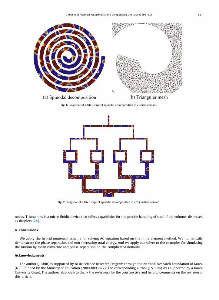
Fig. 6. Snapshot of a later stage of spinodal decomposition in a spiral domain.

Fig. 7. Snapshot of a later stage of spinodal decomposition in a T-junction domain.

J. Shin et al. / Applied Mathematics and Computation 244 (2014) 606–612 611

nodes. T-junctions is a micro-fluidic device that offers capabilities for the precise handling of small fluid volumes dispersedas droplets [24].

4. Conclusions

We apply the hybrid numerical scheme for solving AC equation based on the finite element method. We numericallydemonstrate the phase separation and non-increasing total energy. And we apply our solver to the examples for simulatingthe motion by mean curvature and phase separation on the complicated domains.

Acknowledgments

The author (J. Shin) is supported by Basic Science Research Program through the National Research Foundation of Korea(NRF) funded by the Ministry of Education (2009-0093827). The corresponding author (J.S. Kim) was supported by a KoreaUniversity Grant. The authors also wish to thank the reviewers for the constructive and helpful comments on the revision ofthis article.

612 J. Shin et al. / Applied Mathematics and Computation 244 (2014) 606–612

References

[1] S.M. Allen, J.W. Cahn, A microscopic theory for antiphase boundary motion and its application to antiphase domain coarsening, Acta Metall. 27 (1979)1085–1095.

[2] J.-W. Choi, H.G. Lee, D. Jeong, J. Kim, An unconditionally gradient stable numerical method for solving the Allen–Cahn equation, Physica A 388 (2009)1791–1803.

[3] Y. Li, H.G. Lee, D. Jeong, J.S. Kim, An unconditionally stable hybrid numerical method for solving the Allen–Cahn equation, Comput. Math. Appl. 60(2010) 1591–1606.

[4] X. Feng, H. Wu, A posteriori error estimates and an adaptive finite element method for the Allen–Cahn equation and the mean curvature flow, J. Sci.Comput. 24 (2005) 121–146.

[5] R. Kornhuber, R. Krause, Robust multigrid methods for vector-valued Allen–Cahn equations with logarithmic free energy, Comput. Vis. Sci. 9 (2006)103–116.

[6] A.Q.M. Khaliq, J. Martín-Vaquero, B.A. Wade, M. Yousuf, Smoothing schemes for reaction–diffusion systems with nonsmooth data, J. Comput. Appl.Math. 223 (2009) 374–386.

[7] J. Shen, X. Yang, Numerical approximations of Allen–Cahn and Cahn–Hilliard equations, Discrete Contin. Dyn. Syst. Ser. A 28 (2010) 1669–1691.[8] M. Beneš, V. Chalupecky, K. Mikula, Geometrical image segmentation by the Allen–Cahn equation, Appl. Numer. Math. 51 (2004) 187–205.[9] J.A. Dobrosotskaya, A.L. Bertozzi, A Wavelet-Laplace variational technique for image deconvolution and inpainting, IEEE Trans. Image Process. 17

(2008) 657–663.[10] Z. Rong, L.L. Wang, X.C. Tai, Adaptive wavelet collocation methods for image segmentation using TV–Allen–Cahn type models, Adv. Comput. Math. 38

(2013) 101–131.[11] M. Beneš, K. Mikula, Simulation of anisotropic motion by mean curvature-comparison of phase field and sharp interface approaches, Acta Math. Univ.

Comenian. 67 (1998) 17–42.[12] L.C. Evans, H.M. Soner, P.E. Souganidis, Phase transitions and generalized motion by mean curvature, Commun. Pure Appl. Math. 45 (1992) 1097–1123.[13] X. Feng, A. Prohl, Numerical analysis of the Allen–Cahn equation and approximation for mean curvature flows, Numer. Math. 94 (2003) 33–65.[14] T. Ohtsuka, Motion of interfaces by an Allen–Cahn type equation with multiple-well potentials, Asymptot. Anal. 56 (2008) 87–123.[15] M. Cheng, J.A. Warren, An efficient algorithm for solving the phase field crystal model, J. Comput. Phys. 227 (2008) 6241–6248.[16] A.A. Wheeler, W.J. Boettinger, G.B. McFadden, Phase-field model for isothermal phase transitions in binary alloys, Phys. Rev. A 45 (1992) 7424–7439.[17] L. Blank, M. Butz, H. Garcke, L. Sarbu, V. Styles, Allen–Cahn and Cahn–Hilliard variational inequalities solved with optimization techniques, in: G.

Leugering, S. Engell, M. Hinze, R. Rannacher, V. Schulz, M. Ulbrich, S. Ulbrich (Eds.), Constrained Optimization and Optimal Control for PartialDifferential Equations, ISNM, vol. 160, pp. 21–35, 2012.

[18] J.S. Choi, T. Yamada, K. Izui, S. Nishiwaki, J. Yoo, Topology optimization using a reaction–diffusion equation, Comput. Methods Appl. Mech. Eng. 200(2011) 2407–2420.

[19] X. Yang, J.J. Feng, C. Liu, J. Shen, Numerical simulations of jet pinching-off and drop formation using an energetic variational phase-field method, J.Comput. Phys. 218 (2006) 417–428.

[20] J.H. Adler, J. Brannick, C. Liu, T. Manteuffel, L. Zikatanov, First-order system least squares and the energetic variational approach for two-phase flow, J.Comput. Phys. 230 (2011) 6647–6663.

[21] J. Alberty, C. Carstensen, S.A. Funken, Remarks around 50 lines of Matlab: short finite element implementation, Numer. Algorithms 20 (1999) 117–137.[22] V. Thomee, Galerkin Finite Element Methods for Parabolic Problems, Springer-Verlag, Berlin, 1984.[23] P.C. Fife, Dynamics of Internal Layers and Diffusive Interfaces, SIAM, Philadelphia, PA, 1988.[24] D.R. Link, S.L. Anna, D.A. Weitz, H.A. Stone, Geometrically mediated breakup of drops in microfluidic devices, Phys. Rev. Lett. 92 (2004) 054503.