Embed Size (px)
Citation preview

A HYBRID-PARALLEL FRAMEWORK
FOR THE NONLINEAR SEISMIC ANALYSIS OF VERY TALL BUILDINGS
Thesis by
Abel Bermie R. Dizon
In Partial Fulfillment of the Requirements
for the Degree of
Doctor of Philosophy
California Institute of Technology
Pasadena, California
2016
(Defended December 1, 2015)

ii
© 2016
Abel Bermie R. Dizon
All Rights Reserved

iii
To
Jesus
My wife
My little one

iv
Acknowledgements
I am very blessed to have Dr. John Hall as my advisor. I have learned so much
through my conversations with him. He is encouraging, wise, and patient—qualities I
want to emulate. His clear and logical way of thinking is something I hope to practice
throughout my career. I thank Dr. Swaminathan Krishnan for giving me the opportunity
to pursue this Ph.D. and for teaching me FRAME3D. His guidance through my first two
years at Caltech was indispensable. And I thank Dr. Thomas Sabol from UCLA for being
the first to believe in me as a civil engineer, even while I was a freshman in college. I thank
the members of my candidacy and thesis defense committees: Dr. Domniki Asimaki, Dr.
James Beck, Dr. Thomas Heaton, and Dr. Dennis Kochmann. Their insights are a great
help to this work.
I wish to acknowledge my fellow graduate students, many who helped me
through candidacy and my thesis work. In particular, I thank Pablo Guerrero who studied
with me often during my first year at Caltech. I thank Anthony Massari for conversations
regarding building design and structural engineering in general. It was nice having a
Professional Engineer as a fellow classmate who was willing to help me out as much as
he did. I also thank Kenny Buyco for his help in the final defense preparations.
I am proud to have had the opportunity to study at Caltech, which I consider to
have one of the best learning environments in the world. I am grateful for the financial
support, specifically from the Harold Hellwig Foundation and the George Housner
Fellowship. I thank the administrative staff in the Mechanical and Civil Engineering
Department for all their work.

v
I thank my church communities, NewLife Fellowship and Grace Communion
International Los Angeles, for their prayers, encouragement, and moral support. I
especially thank Dr. Michael Morrison for proofreading this manuscript.
I want to honor my parents Bermie and Carmelita Dizon, who are wonderful
Christ-like role models and who encouraged me to pursue education. I wouldn't be the
man I am today if it wasn't for them. I thank my siblings (and their families) Ben Dizon
and Carmel Benavides, who grew to accept my quirkiness. I am especially glad to have a
brother, David Dizon, who shares my interest in engineering. I thank the Ronquillos, my
wife's family, who welcomed me as a son and brother.
I am very lucky to be married to the love of my life, Ana Dizon. Regarding this
manuscript, I appreciate her help in preparing it. But more importantly, I am grateful that
we are able to share our life-long dreams together. She inspires me to be the best version
of myself, and the last few years would not have been the same without her constant
loving support.
I hope that this work is an inspiration for my future children (such as the little one
on the way), who are already in our hearts and thoughts. I pray that their dreams will
come true, just as my dreams have and continue to come true.
Most of all, I am eternally grateful to my Lord and Savior, Jesus. His guidance
through this life's journey is priceless.

vi
Abstract
FRAME3D, a program for the nonlinear seismic analysis of steel structures, has
previously been used to study the collapse mechanisms of steel buildings up to 20 stories
tall. The present thesis is inspired by the need to conduct similar analysis for much taller
structures. It improves FRAME3D in two primary ways.
First, FRAME3D is revised to address specific nonlinear situations involving large
displacement/rotation increments, the backup-subdivide algorithm, element failure, and
extremely narrow joint hysteresis. The revisions result in superior convergence
capabilities when modeling earthquake-induced collapse. The material model of a steel
fiber is also modified to allow for post-rupture compressive strength.
Second, a parallel FRAME3D (PFRAME3D) is developed. The serial code is
optimized and then parallelized. A distributed-memory divide-and-conquer approach is
used for both the global direct solver and element-state updates. The result is an implicit
finite-element hybrid-parallel program that takes advantage of the narrow-band nature
of very tall buildings and uses nearest-neighbor-only communication patterns.
Using three structures of varied sized, PFRAME3D is shown to compute
reproducible results that agree with that of the optimized 1-core version (displacement
time-history response root-mean-squared errors are ~10−5 m) with much less wall time
(e.g., a dynamic time-history collapse simulation of a 60-story building is computed in
5.69 hrs with 128 cores—a speedup of 14.7 vs. the optimized 1-core version). The
maximum speedups attained are shown to increase with building height (as the total

vii
number of cores used also increases), and the parallel framework can be expected to be
suitable for buildings taller than the ones presented here.
PFRAME3D is used to analyze a hypothetical 60-story steel moment-frame tube
building (fundamental period of 6.16 sec) designed according to the 1994 Uniform
Building Code. Dynamic pushover and time-history analyses are conducted. Multi-story
shear-band collapse mechanisms are observed around mid-height of the building. The use
of closely-spaced columns and deep beams is found to contribute to the building's
“somewhat brittle” behavior (ductility ratio ~2.0). Overall building strength is observed
to be sensitive to whether a model is fracture-capable.

viii
Table of Contents
Acknowledgements ..................................................................................................................... iv
Abstract ......................................................................................................................................... vi
List of Figures ............................................................................................................................ xiii
List of Tables ............................................................................................................................... xix
Chapter 1: Introduction ................................................................................................................ 1
1.1 General ................................................................................................................................. 1
1.2 Literature review ................................................................................................................ 2
1.3 Objectives of the present study ......................................................................................... 5
1.4 Outline of thesis .................................................................................................................. 6
PART I: FRAME3D Reviewed and Revised .............................................................................. 8
Chapter 2: A Review of the FRAME3D Formulation............................................................... 9
2.1 General ................................................................................................................................. 9
2.2 Global solution .................................................................................................................. 11
2.3 Plastic-hinge element ....................................................................................................... 15
2.4 Three-segment elastofiber element ................................................................................ 19
2.5 Five-segment elastofiber element ................................................................................... 27
2.6 Panel-zone element........................................................................................................... 28
2.7 Diaphragm element .......................................................................................................... 31
2.8 Spring element .................................................................................................................. 31
2.9 Conclusion ......................................................................................................................... 32
Chapter 3: Revisions to the FRAME3D Formulation ............................................................. 33
3.1 General ............................................................................................................................... 33
3.2 Large displacement/rotation increments ..................................................................... 37
3.3 The backup-subdivide algorithm ................................................................................... 38
3.4 Element failure .................................................................................................................. 41
3.5 Extremely narrow joint hysteresis .................................................................................. 42

ix
3.6 Demonstration of convergence capabilities .................................................................. 44
3.7 Post-rupture compressive strength ................................................................................ 48
3.8 Conclusion ......................................................................................................................... 50
PART II: A Computationally Efficient, Parallel FRAME3D .................................................. 52
Chapter 4: Overview of Parallel Computing .......................................................................... 53
4.1 General ............................................................................................................................... 53
4.2 Review of parallel computing in structural engineering ............................................ 54
4.3 Terminology ...................................................................................................................... 56
4.4 Parallel performance measures ....................................................................................... 56
4.4.1 General ........................................................................................................................ 56
4.4.2 Wall time ..................................................................................................................... 57
4.4.3 Speedup ...................................................................................................................... 58
4.5 Computer architecture ..................................................................................................... 58
4.6 Speedup strategy .............................................................................................................. 59
Chapter 5: The Direct Solver ..................................................................................................... 63
5.1 General ............................................................................................................................... 63
5.2 Serial (1-core) solvers ....................................................................................................... 66
5.3 Multi-threaded blocked solver ....................................................................................... 71
5.4 Divide-and-conquer solver.............................................................................................. 72
5.5 Conclusion ......................................................................................................................... 83
Chapter 6: Domain Decomposition and Parallel Updating .................................................. 84
6.1 General ............................................................................................................................... 84
6.2 Domain decomposition .................................................................................................... 85
6.2.1 General ........................................................................................................................ 85
6.2.2 DOF allocation ........................................................................................................... 88
6.2.3 Element allocation ..................................................................................................... 89
6.2.4 Node allocation .......................................................................................................... 90
6.2.5 Additional notes ........................................................................................................ 91
6.3 Parallel updating of {𝑏} .................................................................................................... 91
6.3.1 General ........................................................................................................................ 91

x
6.3.2 Parallel updating of {𝑅𝑙}𝑖 ......................................................................................... 93
6.3.3 Parallel updating of ([4
(𝛥𝑡)2𝑀 +
2
𝛥𝑡𝐶] {𝑈𝑙})
𝑖 ........................................................... 98
6.3.4 Parallel updating of other terms in {𝑏}𝑖 ............................................................... 100
6.3.5 Additional notes ...................................................................................................... 100
6.4 Parallel updating of [𝐴] .................................................................................................. 101
6.4.1 General ...................................................................................................................... 101
6.4.2 Parallel updating of [𝐾𝑇𝑙 ]𝑖 ....................................................................................... 101
6.5 Parallel geometric updating .......................................................................................... 102
6.6 Parallel convergence check ............................................................................................ 104
6.7 Parallel input-output ...................................................................................................... 105
6.8 Miscellaneous considerations ....................................................................................... 106
6.8.1 General ...................................................................................................................... 106
6.8.2 Speedup of miscellaneous computational costs .................................................. 107
6.8.3 Load-balancing in the distributed-memory layer ............................................... 108
6.8.4 Conditional multi-threading .................................................................................. 108
6.8.5 Race condition .......................................................................................................... 108
6.8.6 Probabilistic fracture assignments ........................................................................ 109
6.8.7 Shared-memory-only version of PFRAME3D ..................................................... 109
6.9 Conclusion ....................................................................................................................... 109
Chapter 7: Overall Parallelization Results ............................................................................. 111
7.1 General ............................................................................................................................. 111
7.2 Results using a small structure ..................................................................................... 112
7.3 Results using an 18-story building ............................................................................... 116
7.4 Results using a 60-story building simulation ............................................................. 121
7.5 Maximum speedups ....................................................................................................... 127
7.6 Conclusion ....................................................................................................................... 130
PART III: Application and Conclusions ................................................................................ 131
Chapter 8: Application to a 60-story steel building ............................................................. 132
8.1 General ............................................................................................................................. 132
8.2 Building description and design .................................................................................. 133

xi
8.2.1 Building description ................................................................................................ 133
8.2.2 Building design ........................................................................................................ 137
8.3 Modeling considerations ............................................................................................... 142
8.3.1 General ...................................................................................................................... 142
8.3.2 Beams ........................................................................................................................ 142
8.3.3 Columns .................................................................................................................... 144
8.3.4 Beam-column joints ................................................................................................. 144
8.3.5 Floor/roof slabs ....................................................................................................... 144
8.3.6 Foundation ............................................................................................................... 146
8.3.7 Soil-structure interaction ........................................................................................ 146
8.3.8 Gravity loads and mass .......................................................................................... 147
8.3.9 Damping ................................................................................................................... 147
8.3.10 Miscellaneous parameters .................................................................................... 148
8.4 Building analyses and results ....................................................................................... 149
8.4.1 General ...................................................................................................................... 149
8.4.2 Dynamic pushover analysis ................................................................................... 150
8.4.3 Dynamic time-history analysis .............................................................................. 161
Chapter 9: Conclusions and Future Directions ..................................................................... 174
9.1 Conclusions ..................................................................................................................... 174
9.2 Future Directions ............................................................................................................ 178
Appendix A: Computer Architecture .................................................................................... 180
A.1 Terminology ................................................................................................................... 180
A.1.1 General ..................................................................................................................... 180
A.1.2 Hardware................................................................................................................. 181
A.1.3 Software ................................................................................................................... 183
A.2 The cache effect .............................................................................................................. 184
A.3 Regarding GPUs ............................................................................................................ 186
Appendix B: Miscellaneous Parallel Algorithms.................................................................. 187
B.1 Parallel pipelined solver ................................................................................................ 187
B.2 Hybrid-parallel matrix-vector multiplication ............................................................ 191
B.3 Share interface ................................................................................................................ 193

xii
Appendix C: General Behavior of Tube Buildings ............................................................... 194
Appendix D: Non-standard Section Properties .................................................................... 199
Appendix E: Ground Motions ................................................................................................. 201
Bibliography .............................................................................................................................. 206

xiii
List of Figures
Figure 2.1: Example element arrangement in FRAME3D, showing plastic-hinge, three-
segment elastofiber, five-segment elastofiber, panel-zone, and diaphragm elements, with global nodes, local nodes, attachment points, and coordinate systems (Krishnan 2009a, edited). ............................................................................... 11
Figure 2.2: Global DOFs 5 – 8 based on deformations of panel zones (Krishnan 2009a). . 12
Figure 2.3: Nodal forces/moments and displacements/rotations in local coordinates of a plastic-hinge element (Krishnan 2003). ....................................................................... 16
Figure 2.4: Effective shear areas for W-flanged and box sections (Krishnan 2003). .......... 18
Figure 2.5: 𝑃-𝑀𝑝𝑌′ -𝑀𝑝𝑍′ relationships for plastic-hinge elements. 𝑀𝑝𝑌′0 and 𝑀𝑝𝑍′
0 are the
plastic moment capacities when P=0 (top: Krishnan 2003, bottom: Krishnan, 2009b). .............................................................................................................................. 19
Figure 2.6: Three-segment elastofiber element layout (Krishnan 2003). ............................. 20
Figure 2.7: Stress-strain backbone curve of a fiber (Hall and Challa 1995)......................... 23
Figure 2.8: Hysteretic stress-strain paths of a fiber (Hall and Challa 1995). ....................... 24
Figure 2.9: Five-segment elastofiber element layout (Krishnan 2009a). .............................. 28
Figure 2.10: Beam-column joint represented as a panel-zone element (Krishnan 2003). Braces and brace attachment points are not shown. ................................................. 29
Figure 2.11: Shear stress-strain backbone curve of a panel zone (Challa 1992, edited). ... 30
Figure 3.1: Pictorial representation of element-level iterations. Although not pictured, incremental rotations are included in 𝛥𝑈1 and 𝛥𝑈2. ................................................. 35
Figure 3.2: Pictorial representation of a large displacement/rotation increment. Highlighted (grey) is the configuration used by the previous FRAME3D to
construct [KT(k)] for local iteration k=1; the end segments are shown to be highly
deformed. ........................................................................................................................ 37
Figure 3.3: Backup-subdivide algorithm. ................................................................................ 40
Figure 3.4: Joint hysteresis example featuring a negative hysteresis loop branching from a positive panel-zone backbone curve, and a positive hysteresis loop branching from a negative panel-zone backbone curve (Challa 1992, numbers added). ....... 44
Figure 3.5: Unamplified deformations of water-tank tower at t=16 sec (left) and at t=20 sec (right), due to the Kobe earthquake ground motion at Takatori (Figure E.2) scaled to 32%. Failed elements are not shown as they are omitted from analysis. .......................................................................................................................................... 46
Figure 3.6: Water-tank tower roof displacement histories due to the Kobe earthquake

xiv
ground motion at Takatori (Figure E.1), scaled to 32%, as observed by Bjornsson and Krishnan 2014 (solid), and with the §§3.2 – 3.5 revisions (dashed). ............... 47
Figure 3.7: Positive stress-strain backbone curve of a fiber with non-zero post-rupture strength 𝜎𝑓𝑖𝑛 (Challa 1992, post-rupture strength added). ....................................... 49
Figure 3.8: Water-tank tower roof displacement histories, due to the Kobe earthquake ground motion at Takatori (Figure E.1) scaled to 32% and 37.3%, with and without the §3.7 modified backbone curve. ............................................................... 51
Figure 4.1: Wall time (sec) per earthquake-simulation time step from three example collapse simulations: a small (top), a medium (middle), and a large (bottom) system. Part I’s unoptimized FRAME3D is used. ..................................................... 61
Figure 4.2: Computational cost breakdown of significant steps, from 3 collapse simulations. Part I’s unoptimized FRAME3D is used. ............................................. 62
Figure 5.1: Wall times (sec) of serial factorization, using row-based, column-based, and blocked solvers, where m=1000. Intel MKL is used for the “optimized” solvers. 67
Figure 5.2: Wall times (sec) of multi-threaded blocked factorization (dpbtrf) with 1 to 8 cores. Each curve corresponds to a different system size n with m=1000. ............ 72
Figure 5.3: Wall times (sec) of divide-and-conquer factorization with 8 to 256 cores. Each curve corresponds to a different system size n with m=1000. With 8 cores, the multi-threaded blocked factorization from §5.3 is used. A weak-scaling curve (solid green) is constructed (where workload is n = 5000 per 8 cores). ................. 73
Figure 5.4: Wall times (sec) of divide-and-conquer substitution with 8 to 256 cores. Each curve corresponds to a different system size n with m=1000. With 8 cores, the multi-threaded blocked substitution from §5.3 is used. A weak-scaling curve (solid green) is constructed (where workload is 𝑛 = 5000 per 8 cores). ................ 74
Figure 5.5: [A] matrix before divide-and-conquer permutation (Cleary and Dongarra 1997, numbering convention adjusted). Shown are the diagonal and lower half of the matrix. This example uses 4 processes. ................................................................ 77
Figure 5.6: [A] matrix after divide-and-conquer permutation (Cleary and Dongarra 1997, numbering convention adjusted). Shown are the diagonal and lower half of the permuted matrix. This example uses 4 processes. .................................................... 78
Figure 5.7: Local storage of process 2 after divide-and-conquer permutation, before factorization (Cleary and Dongarra 1997). Only the diagonal and lower half of the matrix are stored. ..................................................................................................... 79
Figure 5.8: Local storage of process 2 after the independent portion of factorization (Cleary and Dongarra 1997). Only the diagonal and lower half of the matrix are stored. .............................................................................................................................. 79
Figure 5.9: Final step for the factorization of the “interface” blocks combined as a tridiagonal block system. Shown are the diagonal and lower half of the matrix. This example shows 3 interfaces (4 processes are assumed). .................................. 80

xv
Figure 5.10: Local storage of process 2 at the end of factorization (Cleary and Dongarra 1997, edited). Only the diagonal and lower half of the matrix are stored. ............ 80
Figure 6.1: Domain decomposition of a structure. ................................................................. 86
Figure 6.2: Two-dimensional example illustrating element and node subdomain overlap. The solid lines represent beam elements and the dots represent nodes. The dashed line marks the division between the non-overlapping DOF subdomains of processes i and i+1. The highlighted (grey) elements and nodes belong to both processes 𝑖 and 𝑖 + 1, i.e., are overlapping. ................................................................ 90
Figure 6.3: Wall times (sec) of matrix-vector multiplication with 8 to 128 cores. Each curve corresponds to a different system size n with m=1000. With 8 cores, the multi-threaded matrix-vector routine from Intel MKL (dsbmv) is used. A weak-scaling curve (solid green) is constructed (where workload is 𝑛 = 10,000 per 8 cores). ............................................................................................................................... 96
Figure 6.4: [𝐾]𝑝𝑠 decomposition for hybrid-parallel matrix-vector operation. The thick black lines mark the subdomain divisions. The white portion of the band belongs to [𝐾]𝑝𝑠1 and the grey portion of the band belongs to [𝐾]𝑝𝑠2. Shown are the diagonal and lower half of the matrix. The example uses 4 processes................... 99
Figure 7.1: Isometric views of water-tank tower at t=0 sec (left) and t=38 sec (right) using 37.3% Kobe earthquake ground motion at Takatori (Figure E.1). Elements that failed during analysis are not shown. Deformations are unamplified. ............... 114
Figure 7.2: Roof displacement histories of water-tank tower (from the node initially at X=4.064 m, Y= 8.128 m, Z= 48.768 m) subjected to 37.3% Kobe earthquake ground motion at Takatori (Figure E.1). The results from 1-, 2-, 4-, and 8-core analysis are nearly identical. ............................................................................................................ 115
Figure 7.3: Isometric views of 18-story building at t=0 sec (left) and t=22.7 sec (right) subjected to the acceleration square wave ground motion (Figure E.2). Elements that failed during analysis are not shown. Deformations are unamplified. ........ 118
Figure 7.4: Displacement histories at penthouse roof of 18-story building subjected to an idealized five-cycle acceleration square wave with peak ground velocity PGV=1.375 m⁄s and period T=5.75 sec (Figure E.2). The results from 1-, 8-, 32-, and 48-core analysis are nearly identical. ................................................................. 119
Figure 7.5: Performance summary for 18-story collapse simulation. Wall time of total and various steps (top), and speedup vs. optimized 1-core code (bottom). ........ 120
Figure 7.6: Isometric views of 60-story building at t=0 sec and t=41.9 sec subjected to the Denali earthquake ground motion at Pump Station #10 (Figure E.3). Elements that failed during analysis are not shown. Deformations are unamplified. ........ 124
Figure 7.7: Displacement histories at the roof centroid of the 60-story building subjected to the Denali earthquake ground motion at Pump station #10 (Figure E.3). The results from 1-, 8-, 128-, and 232-core analysis are nearly identical. ..................... 125
Figure 7.8: Performance summary for 60-story collapse simulation. Wall time of total

xvi
and various steps (top), and speedup vs. optimized 1-core code (bottom). ........ 126
Figure 7.9: Wall time (sec) per earthquake-simulation time step, from 60-story building subjected to the Denali earthquake ground motion at Pump station #10 (Figure E.3). PFRAME3D with 128 cores is used. The “spikes” in the {b} & [A] update wall times are a result of load imbalances in the distributed-memory layer (§6.8.3). ........................................................................................................................... 127
Figure 7.10: Summary of “Total” speedups (vs. 1-core) for the water-tank tower, 18-story building, and 60-story building collapse simulations. Also plotted is a curve connecting the maximum speedups achieved for each of the three simulations. ........................................................................................................................................ 129
Figure 8.1: Typical plan (3rd floor to Roof) of 60-story example tube building, featuring closely-spaced columns. .............................................................................................. 134
Figure 8.2: Plan for 2nd floor of 60-story example tube building, featuring transfer girder. ............................................................................................................................ 135
Figure 8.3: Elevation view of the 60-story example building’s first three translational modes along a single direction. ................................................................................. 137
Figure 8.4: Maximum wind drift ratios using ASCE 7-93 (left) and maximum seismic drift ratios using UBC 94 Response Spectrum Method (right) for the 60-story building. ........................................................................................................................ 141
Figure 8.5: Layout of diaphragm elements in a typical floor level. ................................... 145
Figure 8.6: Foundation and soil modeling for 60-story example building. ...................... 146
Figure 8.7: Damping ratio vs. period for 60-story example building. ............................... 148
Figure 8.8: 60-story example building pushover curve (top), base shear history (middle), and roof |X| displacement history (bottom), using perfect welds and three cases of brittle welds. ............................................................................................................. 155
Figure 8.9: Story drift ratios at maximum pushover base shear. Shown are the perfect weld case (left) and the brittle weld case 1 (right). .................................................. 156
Figure 8.10: 60-story example building with perfect welds at ultimate state, t=27.0 sec. Web frame shown on right for the middle portion of the building. Deformations are amplified by 2 for both views. ............................................................................. 157
Figure 8.11: 60-story example building with brittle welds (case 1) at ultimate state, t=18.0 sec. Web frame shown on right for the middle portion of the building. Deformations amplified by 5 for both views. .......................................................... 158
Figure 8.12: Pushover collapse mechanisms of 60-story example building with perfect (left) and brittle (right) welds. Snapshots are taken when nodal displacement exceeds 300 in (~7 m; at t=28.9 sec and t=21.9 sec, respectively). Unamplified deformations shown. Failed elements are not shown as they are omitted from analysis. ......................................................................................................................... 159
Figure 8.13: Illustration showing pure-bending of a beam, from which the relationship

xvii
between fiber strain 𝜀𝑛, fiber position 𝑍𝑛′ (relative to the neutral axis), and
curvature κ can be derived. ........................................................................................ 160
Figure 8.14: Illustration showing that for a given end rotation θ, curvature κ is larger when beam length L is shorter, i.e., because 𝐿1 > 𝐿2, 𝜅1 < 𝜅2. .............................. 160
Figure 8.15: Displacement and drift histories of 60-story example building with perfect welds, subjected to the Denali earthquake ground motion at Pump station #10. ........................................................................................................................................ 165
Figure 8.16: Displacement and drift histories of example 60-story building with brittle welds, subjected to the Denali earthquake ground motion at Pump station #10. ........................................................................................................................................ 166
Figure 8.17: Story drift summary of time-history analysis with perfect (left) and brittle (right) welds. In the left, peak drifts are plotted. In the right, collapse mechanism drifts (at t=30.0 s) are plotted. Shown are drifts in the X (white) and Y (black) directions. ...................................................................................................................... 167
Figure 8.18: 𝑃/𝑃𝑦 histories of 60-story example building with perfect welds, subjected to the Denali earthquake ground motion at Pump station #10. ................................ 168
Figure 8.19: 𝑃/𝑃𝑦 histories of 60-story example building with brittle welds, subjected to the Denali earthquake ground motion at Pump station #10. ................................ 169
Figure 8.20: 𝑀/𝑀𝑝 histories of 60-story example building with perfect welds, subjected to the Denali earthquake ground motion at Pump station #10. ............................ 170
Figure 8.21: 𝑀/𝑀𝑝 histories of 60-story example building with brittle welds, subjected to the Denali earthquake ground motion at Pump station #10. ................................ 171
Figure 8.22: Peak plastic rotations in perfect weld case time-history analysis (due to the Denali earthquake ground motion at Pump Station #10). ..................................... 172
Figure 8.23: Collapse mechanism (at t=30.0 sec) and plastic rotations and flange fractures (right) in brittle weld case time-history analysis (due to the Denali earthquake ground motion at Pump Station #10)........................................................................ 173
Figure A.1: Typical computer cluster schematic with p nodes. ......................................... 182
Figure A.2: Typical schematic of computer node i, featuring dual quad-core processors and three levels of cache. ............................................................................................ 182
Figure B.1: Wall times (sec) of parallel-pipelined factorization with 2 to 64 cores. Each curve corresponds to a different system size n with m=1000. A weak-scaling curve (solid green) is constructed (where workload is n=5000 per core). ........... 190
Figure C.1: Example plan of a moment-frame tube building. ............................................ 196
Figure C.2: Exaggerated fundamental mode of the 60-story example tube building (§8). Compressive flange frame (left), web frame (center), and tensile flange frame (right). ............................................................................................................................ 197
Figure C.3: Upper stories of compressive flange frame. Due to shear lag, outer columns are compressed more than interior columns............................................................ 198

xviii
Figure E.1: Kobe earthquake ground motion at Takatori. Shown are acceleration, velocity, and displacement histories, and pseudoacceleration spectrum. EW, NS, and vertical components are applied along the water-tank tower’s global X, Y, and Z directions, respectively. ................................................................................... 203
Figure E.2: Five-cycle idealized acceleration square wave with peak ground velocity PGV=1.375 m⁄s and period T=5.75 sec. Shown are acceleration, velocity, and displacement histories, and pseudoacceleration spectrum. EW, NS, and vertical components are applied along the 18-story building’s global X, Y, and Z directions, respectively . .............................................................................................. 204
Figure E.3: Denali at Pump Station #10 acceleration, velocity, and displacement histories, and pseudoacceleration spectrum. EW, NS, and vertical components are applied along the 60-story example building’s global X, Y, and Z directions, respectively. ........................................................................................................................................ 205

xix
List of Tables
Table 5.1: Multiplication-division count and storage for LU and Cholesky factorization.
.......................................................................................................................................... 65
Table 5.2: Storage schemes for a banded matrix [A], where * represents symmetry. In this example, n=5 and m=3. ................................................................................................. 68
Table 5.3: Row- and column-based pseudocodes for the serial factorization of a banded positive-definite matrix. ................................................................................................ 68
Table 6.1: Wall time and speedup of parallel {b} calculation, from 60-story dynamic time-history collapse simulation. .......................................................................................... 93
Table 6.2: Wall time and speedup of parallel [A] calculation, from 60-story dynamic time-history collapse simulation. ............................................................................... 102
Table 6.3: Wall time and speedup of geometric updating, from 60-story dynamic time-history collapse simulation. ........................................................................................ 104
Table 6.4: User interface to run FRAME3D and PFRAME3D. In this example, PFRAME3D uses 128 cores (16 processes). Vary “16” to adjust core utilization.106
Table 6.5: Wall time and speedup of miscellaneous computational costs, from 60-story dynamic time-history collapse simulation. .............................................................. 107
Table 7.1: Overall parallelization speedup for water-tank tower collapse simulation. .. 114
Table 8.1: Summary of column and beam sizes for 60-story example building. ............. 136
Table 8.2: Modal periods of 60-story example building. ..................................................... 136
Table 8.3: Design dead loads. .................................................................................................. 138
Table 8.4: ASCE 7-93 wind design parameters for the 60-story example building. ........ 140
Table 8.5: UBC 94 seismic design parameters for the 60-story example building. .......... 141
Table 8.6: Tolerance, convergence, and Newmark parameters .......................................... 149
Table 8.7: 60-story example building pushover results. Roof displacement (m), percent base shear (% of building weight), and ductility ratio (ultimate roof displacement/yield roof displacement). .................................................................. 152
Table 8.8: Summary of plastic rotations from time-history analysis (due to the Denali earthquake ground motion at Pump station #10), with perfect welds. ............... 164
Table A.1: Original and cache-friendly pseudocodes of a 2D matrix update. ................. 185
Table B.1: “Cache-friendly” parallel pipelined factorization*, based on Cho (2012). ..... 188
Table B.2: Benchmark comparison wall times (sec) with the Cho (2012) parallel pipelined solver using n=32,400 and m=8145. .......................................................................... 189

xx
Table B.3: Hybrid-parallel matrix-vector multiplication. .................................................... 192
Table B.4: Share interface routine, used in parallel geometric updating. ......................... 193
Table D.1: Non-standard section properties used in the example 60-story building. ..... 200

1
Chapter 1
Introduction
1.1 General
The structural engineering discipline has greatly been aided by the rise of
structural analysis programs. Today, many such programs like SAP2000, ETABS, RAM,
PERFORM-3D, OpenSees, and LS-DYNA are used by industry and research groups to
solve complex problems. Yet computational challenges limit the capabilities of even the
most popular software packages.
In the past two decades, the California Institute of Technology (Caltech) has
developed FRAME, a program for the nonlinear analysis of steel structures subjected to
2
ground motion. FRAME2D and 3D are capable of simulating building response well up
to the point of collapse. They do this by automatically including in their algorithm
formulations that address the challenges that some programs approach in an ad-hoc
manner, challenges like geometric nonlinearity, robust convergence schemes, weld
fracturing, and material models that match experimental data over many loading cycles.
1.2 Literature review
Of the many structural programs available, PERFORM-3D (CSi 2011) and
OpenSees (Mazzoni et al. 2009) are two of the most widely used programs for highly
nonlinear structural analysis.
PERFORM-3D is a commercial finite-element program, generally considered the
industry standard. It has a large user base among practicing professionals and is suitable
for deformation-based design. Although P-Δ effects are considered, true large-
displacement analysis requires that equilibrium be taken at the structure’s deformed
position, which is not done in PERFORM-3D. Material models are approximated using a
five-line backbone curve, and hysteresis follows these lines. In a study (Bjornsson and
Krishnan 2014) comparing FRAME3D and PERFORM-3D, PERFORM-3D frame elements
were found to deviate from experimental data sooner (fewer loading cycles) than
FRAME3D frame elements. PERFORM-3D also had more difficulty capturing the slow
degradation of structures than FRAME3D.

3
OpenSees is an open-source finite-element program intended for both structural
and geotechnical analysis. Because of its modular design, it has a large element library
and is versatile. This also means that a user determines the level of nonlinearity intended,
the solution algorithms, etc. specific for their project. Features like panel zones, geometric
nonlinearity, large-displacement effects, and strength degradation can be included. The
material models in its database are similar to that of PERFORM-3D, in that they are based
on backbone curves composed of line segments. Although no comparison study between
OpenSees and FRAME3D has been conducted, FRAME3D uses a more realistic steel
backbone and hysteretic material model, and the above features (e.g., panel zones,
geometric nonlinearity, etc.) are automatically included for the context of steel frame
buildings.
The FRAME program is the starting point of the current research. A brief history
of FRAME is presented in the remainder of this section. Recounted are the works of
Caltech professor John Hall and some of his Ph.D. students since the 1990s.
In 1992, Challa completed his thesis, “Nonlinear seismic behavior of steel planar
moment-resisting frames” (Challa 1992). Before this work, the behavior of steel under
cyclic loading was well known from extensive experimental data (e.g., Kent 1969; Popov
and Petersson 1978). Yet few structural analysis programs captured the nonlinear
behavior well over several loading cycles. Challa proposed two computational beam-
column element models: (1), the plastic-hinge element, a simple model, and (2), the fiber
element, a comprehensive model. The plastic-hinge element behaves elastically between
two nodes and is allowed to hinge plastically when end moments exceed a yield value. It
accounts for strain hardening approximately by including an elastic rotational spring after

4
hinging occurs. The more robust fiber element is discretized transversely into subelements
(i.e., segments), where each segment is discretized longitudinally into fibers. Each fiber
follows the backbone curve and hysteretic rules of a steel bar under uniaxial stress, based
on experimental data (Kent 1969; Popov and Petersson 1978). The joints of the frames have
finite size and match the experimental shear stress-strain curves well (Tsai and Popov
1988). Additionally, Newmark’s method (Newmark 1959) was used to solve the
incremental equations of motion (§2.2). The result of this work was the NDA2 program, a
precursor to FRAME2D.
Hall and Challa developed and published the formulation of FRAME2D (Hall and
Challa 1995). The 1994 Northridge earthquake revealed a flaw in pre-Northridge moment-
resisting buildings: welds fractured below design levels. Thus, the fiber formulation was
updated to simulate weld fractures (Hall 1995; Hall 1998).
In the first efforts to extend FRAME2D to three dimensions, Carlson and Hall
developed a 3D fiber discretization of columns and a 3D joint (Carlson and Hall 1997).
Carlson also developed 3D constraint equations that represent the effect of rigid
diaphragms, so that a 3D building can be studied using planar frames. The work resulted
in the ANDERS program and Carlson’s thesis “Three dimensional nonlinear inelastic
analysis of steel moment-frame buildings damaged by earthquake excitations” (Carlson
1999). Carlson compared fracture-incapable models with fracture-capable models and
found little correlation between their behaviors, which suggests that for large motions,
fracture-incapable models would be insufficient. ANDERS, however, was not “fully 3D”;
it neglected some 3D effects such as the biaxial bending of non-corner columns.

5
Krishnan reformulated FRAME2D into FRAME3D, fully accounting for 3D effects.
He examined irregularly shaped buildings, those with a center of mass and rigidity that
do not coincide, and observed that torsional demand can be significant. He documented
the 3D transition in his thesis “Three dimensional nonlinear analysis of tall irregular steel
buildings subject to strong ground motion” (Krishnan 2003). A 3D analog replaced every
2D element. For example, 3D plastic-hinge elements can hinge in two orthogonal
directions. 3D fiber segments are discretized to account for biaxial bending. For
computational efficiency, Krishnan introduced the three-segment elastofiber element,
which was calibrated to replace the fiber element. The descriptions and formulations of
the 3D plastic-hinge and three-segment elastofiber elements can be found in §2.3 and §2.4,
respectively.
In 2009, Krishnan added the five-segment elastofiber element to FRAME3D’s
element library to efficiently capture geometric nonlinearities and buckling. A description
and formulation of the five-segment elastofiber element can be found in §2.5.
1.3 Objectives of the present study
Since the 1990s, FRAME2D and FRAME3D have contributed to the structural
engineering community’s knowledge of steel frame buildings up to 20 stories, their
response in strong earthquakes, and their collapse mechanisms. The primary goal of the
current thesis is to extend the capability of FRAME3D to steel buildings much taller than
20 stories. It is achieved with the following intermediate objectives:

6
Review the existing formulation of FRAME3D. It is important to understand
how the program works before improving it.
Propose revisions to the formulation of FRAME3D. The goal of these revisions
is to improve the program’s ability to handle highly nonlinear situations, such
as building collapse, and improve the realism of the steel material model.
Develop a computationally efficient, parallel FRAME3D. FRAME3D’s
nonlinear formulation is complex and detailed enough that for systems larger
than 20 stories, a sequential dynamic time-history collapse simulation may
take days or weeks complete. This thesis aims to significantly reduce the
computation times of tall-building simulations.
Develop and study an example 60-story steel building. The primary purpose
of this example is to showcase PFRAME3D’s computational performance. A
secondary purpose is to analyze the 60-story building’s nonlinear behavior and
collapse mechanisms. (The secondary purpose will be achieved with greater
detail in future work.)
1.4 Outline of thesis
This thesis consists of three parts.
Part I presents a review of and the revisions to FRAME3D's formulations. Chapter
2 reviews the FRAME3D formulation. It covers the global equations of motion and the

7
element contributions to the equations. Chapter 3 presents revisions to the FRAME3D
formulation, including their effect on improving the robustness of the program.
Part II focuses on the development of the parallel version of FRAME3D. Chapter 4
provides a general orientation to parallel computing. Chapter 5 discusses the direct solver.
Several algorithms are considered and a divide-and-conquer solver is chosen for
PFRAME3D. Chapter 6 covers domain decomposition and parallel updating. Chapter 7
demonstrates that PFRAME3D produces nearly identical results as FRAME3D in
significantly less time.
Part III covers the application of PFRAME3D to a 60-story example building.
Chapter 8 explains the design considerations according to pre-Northridge (UBC 94)
provisions, the modeling considerations for creating the PFRAME3D model, and the
results of dynamic pushover and dynamic time history analysis. Finally, Chapter 9 is the
conclusion of this report and presents future directions.

8
PART I
FRAME3D Reviewed and Revised

9
Chapter 2
A Review of the
FRAME3D Formulation
2.1 General
A structural finite element program works by defining a set of elements connected
at nodes, and then solving equations of equilibrium that describe how those elements
respond to external input generally applied at the nodes. For a 2D model, the elements lie
on a plane; for a 3D model, they lie in 3D space. The equations of equilibrium depend on
many variables—such as element properties, model geometry, boundary conditions—and

10
for dynamic problems, mass, damping, and initial conditions, too. A review of
FRAME3D’s equations is the focus of this chapter.
The discussion here begins with the global equation of motion (§2.2) and ends with
how each type of element contributes to the global equation (§§2.3 – 2.8).
The element library consists of:
the plastic-hinge element (§2.3)
the three-segment elastofiber element (§2.4)
the five-segment elastofiber element (§2.5)
the panel-zone element (§2.6)
the four-noded diaphragm element (§2.7)
the translational/rotational spring element (§2.8).
An example arrangement of these elements (except the spring) is shown in Figure 2.1 to
provide context. Three right-handed orthogonal coordinate systems are used: (1) the
global 𝑋𝑌𝑍 system, where 𝑋 and 𝑌 are horizontal and 𝑍 is vertical; (2) the panel-zone �̅��̅��̅�
system, where �̅�, �̅�, and �̅� are initially defined to match the longitudinal, major, and minor
axes, respectively, of the panel zone’s “associated column” (typically the column
immediately beneath the panel zone); and, (3) the beam segment/element 𝑋′𝑌′𝑍′ system,
where 𝑋′, 𝑌′, and 𝑍′ are the longitudinal, major, and minor axes, respectively, of the beam
segment/element chord. The coordinate systems, elements, and nodes are further
explained in §2.2 – 2.8. In-depth explanations can be found in Krishnan (2003), Krishnan
and Hall (2006a, 2006b), and Krishnan (2009a).

11
Figure 2.1: Example element arrangement in FRAME3D, showing plastic-hinge, three-segment
elastofiber, five-segment elastofiber, panel-zone, and diaphragm elements, with global nodes, local
nodes, attachment points, and coordinate systems (Krishnan 2009a, edited).
2.2 Global solution
The dynamic solution of FRAME3D is based on the matrix equation (Cook et al.
1989):
[𝑀]{�̈�(𝑡)} + [𝐶]{�̇�(𝑡)} + {𝑅(𝑡)} = {𝑓𝑔} − [𝑀][𝑟]{�̈�𝑔(𝑡)} (Eq. 2.1)
where {�̈�(𝑡)} and {�̇�(𝑡)} are vectors of global accelerations and velocities, respectively,
over time ({𝑈(𝑡)}, not shown in Eq. 2.1, is a vector of global displacements); [𝑀] is the

12
mass matrix, diagonal because masses are lumped at global nodes; [𝐶] is the Rayleigh
damping matrix: [𝐶] = 𝑎0[𝑀] + 𝑎1[𝐾], where [𝐾] is the initial elastic stiffness matrix and
𝑎0 & 𝑎1 are Rayleigh damping parameters; {𝑅(𝑡)} is the vector of nonlinear stiffness forces
(i.e., internal or restoring forces); {𝑓𝑔} is the static external force vector, typically of gravity
forces; {�̈�𝑔(𝑡)} is the three-component (global 𝑋, 𝑌, and 𝑍) input ground motion vector;
and [𝑟] is the participation matrix (so that {�̈�𝑔(𝑡)} can be applied as inertial forces through
[𝑀]).
In 3D, {𝑈(𝑡)}, {�̇�(𝑡)}, {�̈�(𝑡)}, {𝑅(𝑡)}, etc. have 6 to 8 degrees of freedom (DOFs) per
node. At each node, DOFs 1 – 3 are translations in global 𝑋, 𝑌, and 𝑍 directions (Figure
2.1). DOF 4 is the rigid body rotation of the panel-zone element about the �̅� axis (Figure
2.1). DOFs 5 – 8 define the deformations of the 2 orthogonal panel zones; each panel zone
can deform in 2 modes (Figure 2.2). When one or both panel zones are absent or rigid,
DOFs 5 – 6 and DOFs 7 – 8 consolidate to define up to 2 rigid body rotations, i.e., the node
has 6 or 7 DOFs instead of 8. It should be noted that the global rotational DOFs are not
about the fixed global axes 𝑋𝑌𝑍, but rather are defined by the panel-zone �̅��̅��̅� system.
Figure 2.2: Global DOFs 5 – 8 based on deformations of panel zones (Krishnan 2009a).

13
Discretizing time (𝛥𝑡), applying constant average acceleration, and recognizing
that a time step often cannot be completed in a single iteration, Eq. 2.1 at global iteration
𝑙 of time step 𝑡 becomes
[4
(𝛥𝑡)2𝑀+
2
𝛥𝑡𝐶 + 𝐾𝑇
𝑙 ] {𝛥𝑈} = {𝑓𝑔} − {𝑅𝑙} − [𝑀][𝑟]{�̈�𝑔(𝑡)} (Eq. 2.2)
+[𝑀] {4
(𝛥𝑡)2𝑈(𝑡) +
4
𝛥𝑡�̇�(𝑡) + �̈�(𝑡)}
+[𝐶] {2
𝛥𝑡𝑈(𝑡) + �̇�(𝑡)} − [
4
(𝛥𝑡)2𝑀+
2
𝛥𝑡𝐶] {𝑈𝑙}
where [𝐾𝑇𝑙 ] is the global iterating matrix. Although the subscript 𝑇 suggests that [𝐾𝑇
𝑙 ] is a
“tangent stiffness matrix,” it includes an elastic term, too; also, the fiber material model
may use non-tangent slopes (discussed more in §2.4); and, because analysis is dynamic,
whether an element loads or unloads is not necessarily certain at a given global iteration;
thus, the true “tangent stiffness matrix” is often not used.
[𝐾𝑇𝑙 ], {𝛥𝑈}, {𝑈𝑙}, and {𝑅𝑙} are updated in every iteration. {𝑈(𝑡)}, {�̇�(𝑡)}, {�̈�(𝑡)}, and
{�̈�𝑔(𝑡)} are updated at the beginning of every time step. [𝑀], [𝐶], and {𝑓𝑔} are constant
throughout the dynamic analysis.
A typical global iteration 𝑙 follows these steps:
(0) Get the right-hand side (RHS) using iteration 𝑙 − 1 or the previous time step.
The RHS is known as the force residual, which physically represents the
difference between internal and external forces (including dynamic effects) at
every DOF at the current global iteration.
(1) Check convergence. The system is considered to be converged if the infinity
norm of the RHS is nearly zero, within a tolerance. Physically, a zeroed infinity
norm implies dynamic force equilibrium at every node. If the system

14
converged, proceed to the next time step; the current configuration {𝑈𝑙} is
regarded as the solution for the current time step {𝑈(𝑡 + 𝛥𝑡)}. If the system did
not converge, continue iterating.
(2) Assemble [𝐾𝑇𝑙 ], the tangent stiffness matrix, based on every element in the
structure, and on the nodal configuration at iteration 𝑙. Add [𝐾𝑇𝑙 ] to the
constant 4
(𝛥𝑡)2[𝑀] and
2
𝛥𝑡[𝐶] terms to get the left-hand side (LHS) matrix
[4
(𝛥𝑡)2𝑀+
2
𝛥𝑡𝐶 + 𝐾𝑇
𝑙 ].
(3) Solve for {𝛥𝑈} using the LHS matrix and the RHS. {𝛥𝑈} represents the
incremental difference between {𝑈𝑙} and {𝑈𝑙+1}. The solution process has two
parts:
a. Factor the LHS matrix with Cholesky or 𝐿𝐷𝐿𝑇 factorization.
b. Solve the factored system.
For more details on this step, see §5.
(4) Update the geometry of the system—including element geometric parameters,
nodal locations/attachment points, and {𝑈𝑙+1}. This updated geometry will be
used at the next convergence check (step 1 of global iteration 𝑙 + 1). Because of
this step, geometric nonlinearities and P-Δ effects are automatically included.
(5) Assemble {𝑅𝑙+1}, the internal force vector, based on every element in the
structure, and on the updated 𝑙 + 1 geometry. Go to iteration 𝑙 + 1.
The primary task at each global iteration is to update [𝐾𝑇𝑙 ] and {𝑅𝑙}, both of which are
assembled from finite elements (§§2.3 – 2.8). For each element in the model, a static
specified-displacement problem is solved; i.e., given an incremental displacement {𝛥𝑈},

15
element stiffness and internal forces are determined such that static equilibrium is
satisfied. The individual element contributions are combined to form [𝐾𝑇𝑙 ] and {𝑅𝑙}. The
remainder of this chapter covers, for each element type, the formulations of these “local”
calculations.
2.3 Plastic-hinge element
The plastic-hinge (PH) element is a computationally efficient element, useful for
preliminary analysis or for modeling secondary elements. Its formulation assumes doubly
symmetric cross sections, centroidal axes, uniform cross sections along element length,
and no warping restraint. The 12-DOF equation (6 DOFs per node) in incremental form
describes the element:
{𝑑𝑅𝑝ℎ′ }
𝐿= [𝐾𝑇,𝑝ℎ
′ ]𝐿{𝑑𝑈𝑝ℎ
′ }𝐿 (Eq. 2.3)
where {𝑑𝑅𝑝ℎ′ }
𝐿, [𝐾𝑇,𝑝ℎ
′ ]𝐿, and {𝑑𝑈𝑝ℎ
′ }𝐿 are the element’s incremental internal force vector,
tangent stiffness matrix, and incremental displacement, respectively, in its local 𝑋’𝑌’𝑍’
coordinate system (§2.1; Figure 2.1). The 6 DOFs per node are 3 translational and 3
rotational DOFs, as indicated by the subscript 𝐿. Before Eq. 2.3 is solved, the global
displacement increments {𝛥𝑈𝑝ℎ} (extracted from {𝛥𝑈}) are transformed to {𝛥𝑈𝑝ℎ′ }
𝐿 using
{𝛥�̅�𝑝ℎ} = [𝑇1]{𝛥𝑈𝑝ℎ} (Eq. 2.4)
{𝛥�̅�𝑝ℎ}𝐿 =[𝑇2]{𝛥�̅�𝑝ℎ} (Eq. 2.5)
{𝛥𝑈𝑝ℎ}𝐿 =[𝑇3]{𝛥�̅�𝑝ℎ}𝐿 (Eq. 2.6)

16
{𝛥𝑈𝑝ℎ′ }
𝐿= [𝑇4]{𝛥𝑈𝑝ℎ}𝐿
(Eq. 2.7)
where [𝑇1] transforms the global displacement increments from the 𝑋𝑌𝑍 to the �̅��̅��̅�
system; [𝑇2] from the global node (e.g., J & K in Figure 2.1) to the local attachment point
(e.g., 1 & 2 in Figure 2.1), which reduces the number of DOFs per node from 6 – 8 to 6 as
denoted by the subscript 𝐿; [𝑇3] from the �̅��̅��̅� system to the 𝑋𝑌𝑍 system; and [𝑇4] from the
𝑋𝑌𝑍 system to the 𝑋′𝑌′𝑍′ system. The result of the transformations is {𝑑𝑈𝑝ℎ′ }
𝐿. {𝑑𝑅𝑝ℎ
′ }𝐿 and
[𝐾𝑇,𝑝ℎ′ ]
𝐿 are determined from {𝑑𝑈𝑝ℎ
′ }𝐿 using Eq. 2.8 – 2.10, and are transformed back to the
6 – 8 DOFs per node in the global 𝑋𝑌𝑍 system.
Figure 2.3: Nodal forces/moments and displacements/rotations in local coordinates of a plastic-
hinge element (Krishnan 2003).

17
Each term in {𝑑𝑅𝑝ℎ′ }
𝐿and [𝐾𝑇,𝑝ℎ
′ ]𝐿 is computed from beam theory, and accounts for
axial, flexural, shear, and twisting contributions (Figure 2.3). Axial (𝑃, 𝑈) and twisting (𝑇,
𝛼) contributions come from:
{𝑑𝑃1𝑑𝑃2
} =𝐸𝑇𝐴
𝐿0[1 −1−1 1
] {𝑑𝑈1𝑑𝑈2
} (Eq. 2.8)
{𝑑𝑇1𝑑𝑇2
} =𝐺𝐽
𝐿0[1 −1−1 1
] {𝑑𝛼1𝑑𝛼2
} (Eq. 2.9)
where the subscripts 1 and 2 denote the local element node number; 𝐸𝑇 is the tangent
Young’s modulus as independently computed using axial force only; 𝐴 is the cross
sectional area; 𝐿0 is the original element length; 𝐺 is the elastic shear modulus; and 𝐽 is the
torsional inertia. 𝐸𝑇 is determined by a bilinear material model defined by the elastic
modulus 𝐸, the yield stress 𝜎𝑦, and the strain-hardening (i.e., post-yield) modulus 𝐸𝑠ℎ,
and unloading is elastic. Eq. 2.9 neglects warping restraint. The flexural (𝑀, 𝜃) and shear
(𝑄, 𝑉) contributions about the major axis (𝑌′) come from:
{
𝑑𝑄1𝑍′
𝑑𝑀1𝑌′
𝑑𝑄2𝑍′
𝑑𝑀2𝑌′}
=
[
[ −1
𝐿01
−1
𝐿00
1
𝐿00
1
𝐿01 ]
[𝑎𝑇 𝑏𝑇𝑏𝑇 𝑐𝑇
]
[ −1
𝐿01
1
𝐿00
−1
𝐿00
1
𝐿01]
+𝑃
𝐿0[
1 00 0
−1 00 0
−1 00 0
1 00 0
]
]
{
𝑑𝑉1𝑍′
𝑑𝜃1𝑌′
𝑑𝑉2𝑍′
𝑑𝜃2𝑌′}
(Eq. 2.10)
where 𝑎𝑇, 𝑏𝑇, and 𝑐𝑇 depend on 𝐸, 𝐺, 𝑃, major-axis moment of inertia 𝐼𝑌′, major-axis
effective shear area 𝐴𝑆𝑍′ (Figure 2.4), and major-axis plastic-hinge conditions at nodes 1
and 2 (Krishnan 2003; Krishnan and Hall 2006a).

18
Figure 2.4: Effective shear areas for W-flanged and box sections (Krishnan 2003).
A plastic hinge occurs when the moment at node 1 or 2 exceeds the yield moment
𝑀𝑝𝑌′ or 𝑀𝑝𝑍′ as defined by a 𝑃-𝑀𝑝𝑌′-𝑀𝑝𝑍′ (PMM) interaction relationship. FRAME3D has
two types of interaction curves. The first, shown in Figure 2.5 (top), accounts for the effect
of 𝑃 on the plastic moment capacities, but not the effect of major-axis bending on minor-
axis plastic moment capacity and vice versa. The second is a PMM surface, constructed
from a user-defined section (Krishnan 2009b); e.g., the PMM interaction relationship for a
W6X20 section is shown in Figure 2.5 (bottom). Between nodes, the element is elastic in
flexure. Switch 𝑍′ and 𝑌′ in Eq. 2.10 to get the flexural and shear formulation about the
minor axis. The PH element, although efficient, is suited for secondary and pinned
elements. To more accurately capture beam behavior for high levels of inelasticity, a more
complicated fiber-based element is required.
The next two sections describe the formulation of two fiber-based elements: the
three-segment and five-segment elastofiber elements.

19
Figure 2.5: 𝑃-𝑀𝑝𝑌′ -𝑀𝑝𝑍′ relationships for PH elements. 𝑀𝑝𝑌′0 and 𝑀𝑝𝑍′
0 are the plastic moment
capacities when P=0 (top: Krishnan 2003, bottom: Krishnan, 2009b).
2.4 Three-segment elastofiber element
The three-segment elastofiber (EF3) element is suited for accurately modeling
beams over many loading cycles. It can capture flexural behavior similar to a fully
20
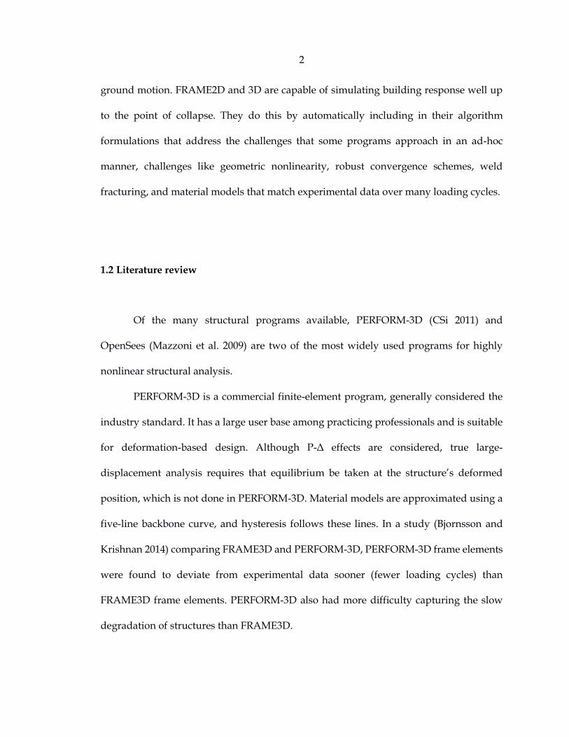
discretized fiber element with significantly less computational cost (Krishnan 2003). It
consists of 3 segments (fiber-elastic-fiber) and 4 nodes (2 interior and 2 exterior) (Figure
2.6).
Figure 2.6: Three-segment elastofiber element layout (Krishnan 2003).
21
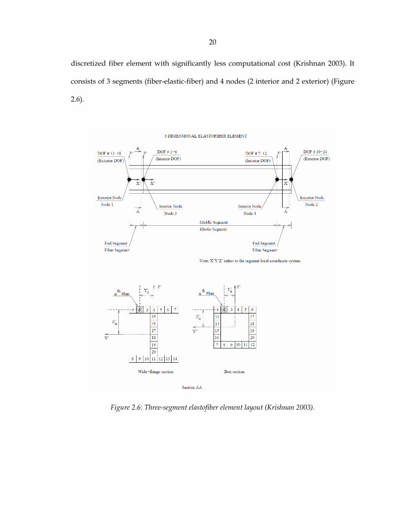
Because displacement increments are specified at the exterior nodes and the EF3
element has 2 interior nodes, it is treated like a local structural analysis problem. Thus,
Newton-Raphson iterations (Eq. 2.11; similar to §2.2) are used to achieve local force
equilibrium. For local iteration (𝑘),
[𝐾𝑇,𝐼𝐼(𝑘) 𝐾𝑇,𝐼𝐸
(𝑘)
𝐾𝑇,𝐸𝐼(𝑘)
𝐾𝑇,𝐸𝐸(𝑘)
] {𝛥𝑈𝐼𝛥𝑈𝐸
} = {0𝐹𝐸} − {
𝑅𝐼(𝑘)
𝑅𝐸(𝑘)} (Eq. 2.11)
where the (𝑘) denotes local iterations within global iteration l; the subscripts 𝐼 and 𝐸
indicate the 12 internal and 12 external DOFs, respectively, of the EF3 element (6 DOFs
per node using the 𝑋𝑌𝑍 system); {𝛥𝑈𝐸} is the known displacement increment {𝛥𝑈𝑒𝑓}𝐿
applied at the exterior nodes (transformed from {𝛥𝑈𝑒𝑓} using [𝑇1], [𝑇2], and [𝑇3]); {𝐹𝐸}
represents unknown external forces (which can be ignored as shown in Eq. 2.12 – 2.13);
[𝐾𝑇,𝐼𝐼(𝑘) 𝐾𝑇,𝐼𝐸
(𝑘)
𝐾𝑇,𝐸𝐼(𝑘)
𝐾𝑇,𝐸𝐸(𝑘)
] and {𝑅𝐼(𝑘)
𝑅𝐸(𝑘)} are assembled from segment contributions (after the
contributions are transformed using [𝑇4] from segment 𝑋′𝑌′𝑍′ systems to the 𝑋𝑌𝑍 system);
and {𝛥𝑈𝐼} is solved from
[𝐾𝑇,𝐼𝐼(1)] {𝛥𝑈𝐼} = − [𝐾𝑇,𝐼𝐸
(1)] {𝛥𝑈𝐸} − {𝑅𝐼
(1)} (Eq. 2.12)
[𝐾𝑇,𝐼𝐼(𝑘)] {𝛥𝑈𝐼} = − {𝑅𝐼
(𝑘)}. (Eq. 2.13)
In Eq. 2.12, i.e., (𝑘) = 1, the effect of {𝛥𝑈𝐸} is an applied force on the upper 𝐼 equations of
Eq. 2.11. At local convergence, the internal DOFs are condensed out of [𝐾𝑇,𝐼𝐼(𝑘) 𝐾𝑇,𝐼𝐸
(𝑘)
𝐾𝑇,𝐸𝐼(𝑘) 𝐾𝑇,𝐸𝐸
(𝑘)] and
{𝑅𝐼(𝑘)
𝑅𝐸(𝑘)} using partial factorization, resulting in [𝐾𝑇,𝑒𝑓
𝑙+1 ]𝐿 and {𝑅𝑒𝑓
𝑙+1}𝐿, which are then

22
transformed into [𝐾𝑇,𝑒𝑓𝑙+1 ] and {𝑅𝑒𝑓
𝑙+1} using [𝑇3], [𝑇2], and [𝑇1], and assembled into the global
[𝐾𝑇𝑙+1] and {𝑅𝑙+1} arrays.
[𝐾𝑇,𝐼𝐼(𝑘)
𝐾𝑇,𝐼𝐸(𝑘)
𝐾𝑇,𝐸𝐼(𝑘)
𝐾𝑇,𝐸𝐸(𝑘)
] and {𝑅𝐼(𝑘)
𝑅𝐸(𝑘)} are assembled from segment contributions. The center
segment has an elastic beam formulation, without axial yielding or plastic hinging
capabilities. The two outer fiber segment formulations can be derived from individual
fibers (Figure 2.6).
Consider fiber 𝑛 in a segment. Fiber 𝑛 has an incremental strain 𝑑𝜀𝑛 that depends
on the incremental (axial) translations 𝑑𝑈 and incremental (relative to the chord) rotations
𝑑𝜑 of the segment nodes 𝑖, 𝑗:
𝑑𝜀𝑛 =𝑑𝑈𝑗−𝑑𝑈𝑖
𝐿𝑠0+
𝑍𝑛′ (𝑑𝜑
𝑗𝑌′−𝑑𝜑
𝑖𝑌′)
𝐿𝑠0−
𝑌𝑛′(𝑑𝜑
𝑗𝑍′−𝑑𝜑
𝑖𝑍′)
𝐿𝑠0 (Eq. 2.14)
where 𝑍𝑛′ and 𝑌𝑛
′ is the location of fiber 𝑛 along the cross section (Figure 2.6), and 𝐿𝑠0 is
the original segment length.
A robust material model (Figure 2.7 and Figure 2.8, Hall and Challa 1995) defines
the fiber’s current tangent stiffness 𝐸𝑇,𝑛 and stress 𝜎𝑛 based on its stress-strain history and
𝑑𝜀𝑛. The user-defined backbone curve has an initial elastic region, a yield plateau, and a
strain-hardening/softening curve defined by a cubic ellipse. In this curve, 𝐸 is the elastic
modulus, 𝜎𝑦 is the yield stress, 𝐸𝑠ℎ is the tangent modulus at the onset of strain-hardening,
𝜀𝑠ℎ is the strain at the onset of strain-hardening, 𝜎𝑢 is the ultimate stress, and 𝜀𝑢 is the fiber
ultimate strain. The cubic ellipse (𝜀, 𝜎) in Figure 2.7 is determined by
(𝜀−𝜀0)
3
𝑎3+
(σ−𝜎0)3
𝑏3= 1 (Eq. 2.15)

23
where 𝜀0 and 𝜎0 define the center of the ellipse, and 𝑎 and 𝑏 are the diameters of the ellipse.
𝜀0, 𝜎0, 𝑎, and 𝑏 are functions of 𝜎𝑦, 𝐸𝑠ℎ, 𝜀𝑠ℎ, 𝜎𝑢, and 𝜀𝑢. At the plateau region of the
backbone curve (between point A and the point of strain-hardening onset in Figure 2.7),
𝐸𝐴𝐵 is used as 𝐸𝑇,𝑛, where the A-B line segment is tangent to the cubic ellipse at point B.
Beyond the ultimate point (between points C and D in Figure 2.7), 0 is used as 𝐸𝑇,𝑛. The
Extended Masing’s hypothesis, described in Challa (1992), governs the hysteretic behavior
(Figure 2.8). Fibers may also fracture in tension if a predetermined probabilistic fracture
strain is exceeded; a fractured fiber may carry compressive loads.
Figure 2.7: Stress-strain backbone curve of a fiber (Hall and Challa 1995).

24
Figure 2.8: Hysteretic stress-strain paths of a fiber (Hall and Challa 1995).
Fiber contributions are combined to get the segment’s incremental axial force (𝑑𝑃)
and moment (𝑑𝑀):
𝑑𝑃 = ∑ 𝐸𝑇,𝑛𝐴𝑛𝑑𝜀𝑛𝑛 (Eq. 2.16)
𝑑�̅�𝑌′ = −∑ 𝐸𝑇,𝑛𝐴𝑛𝑍𝑛′
𝑛 𝑑𝜀𝑛 (Eq. 2.17)
𝑑�̅�𝑍′ = ∑ 𝐸𝑇,𝑛𝐴𝑛𝑌𝑛′
𝑛 𝑑𝜀𝑛 (Eq. 2.18)
where 𝐴𝑛 is fiber area. The overbar indicates that 𝑑𝑀 corresponds to the segment center.
Shear (𝑑𝑄) is elastic and computed independently:
𝑑�̅�𝑌′ = −𝐴𝑆𝑌′𝐺(𝑑𝜑
𝑖𝑍′+𝑑𝜑
𝑗𝑍′)
2 (Eq. 2.19)
𝑑�̅�𝑍′ = 𝐴𝑆𝑍′𝐺(𝑑𝜑
𝑖𝑌′+𝑑𝜑
𝑗𝑌′)
2 (Eq. 2.20)

25
where 𝐴𝑆𝑌′ and 𝐴𝑆𝑍′ are the cross-sectional shear areas (Figure 2.4). Twisting (𝑑𝑇) is
computed in the same way as PH element twisting. Eq. 2.14 is substituted into Eq. 2.16 –
2.20, and Eq. 2.16 – 2.20 and Eq. 2.9 are combined to form the matrix equation
{
𝑑𝑃𝑑�̅�𝑌′
𝑑�̅�𝑍′
𝑑�̅�𝑌′
𝑑�̅�𝑍′
𝑑𝑇 }
= [𝐶𝑇]
{
𝑑𝑈𝑗−𝑑𝑈𝑖
𝐿𝑠0
−𝑑𝜑
𝑗𝑌′−𝑑𝜑
𝑖𝑌′
𝐿𝑠0
−𝑑𝜑
𝑗𝑍′−𝑑𝜑
𝑖𝑍′
𝐿𝑠0
−𝑑𝜑
𝑖𝑍′+𝑑𝜑
𝑗𝑍′
𝐿𝑠0𝑑𝜑
𝑖𝑌′+𝑑𝜑
𝑗𝑌′
𝐿𝑠0𝑑𝛼𝑗−𝑑𝛼𝑖
𝐿𝑠0 }
(Eq. 2.21)
where
[𝐶𝑇] =
[ ∑ 𝐸𝑇,𝑛𝐴𝑛𝑛 −∑ 𝐸𝑇,𝑛𝐴𝑛𝑍𝑛
′𝑛 ∑ 𝐸𝑇,𝑛𝐴𝑛𝑌𝑛
′𝑛 0 0 0
∑ 𝐸𝑇,𝑛𝐴𝑛𝑍𝑛′2
𝑛 −∑ 𝐸𝑇,𝑛𝐴𝑛𝑌𝑛′𝑍𝑛
′𝑛 0 0 0
∑ 𝐸𝑇,𝑛𝐴𝑛𝑌𝑛′2
𝑛 0 0 0
symmetric 𝐴𝑆𝑌′𝐺 0 0
𝐴𝑆𝑍′𝐺 0
𝐺𝐽]
. (Eq. 2.22)
By substituting
{
𝑑𝑈𝑗−𝑑𝑈𝑖
𝐿𝑠0
−𝑑𝜑
𝑗𝑌′−𝑑𝜑
𝑖𝑌′
𝐿𝑠0
−𝑑𝜑
𝑗𝑍′−𝑑𝜑
𝑖𝑍′
𝐿𝑠0
−𝑑𝜑
𝑖𝑍′+𝑑𝜑
𝑗𝑍′
𝐿𝑠0𝑑𝜑
𝑖𝑌′+𝑑𝜑
𝑗𝑌′
𝐿𝑠0𝑑𝛼𝑗−𝑑𝛼𝑖
𝐿𝑠0 }
=1
𝐿𝑠0[𝑆]
{
𝑑𝑈𝑖𝑑𝑉𝑖𝑌′
𝑑𝑉𝑖𝑍′
𝑑𝛼𝑖𝑑𝜃𝑖𝑌′
𝑑𝜃𝑖𝑍′
𝑑𝑈𝑗𝑑𝑉𝑗𝑌′
𝑑𝑉𝑗𝑍′
𝑑𝛼𝑗𝑑𝜃𝑗𝑌′
𝑑𝜃𝑗𝑍′}
(Eq.2.23)
where

26
[𝑆] =
[ −1 0 0 0 0 0 1 0 0 0 0 00 0 0 0 1 0 0 0 0 0 −1 00 0 0 0 0 1 0 0 0 0 0 −1
0 −1 0 0 0 −𝐿𝑠0
20 1 0 0 0 −
𝐿𝑠0
2
0 0 −1 0𝐿𝑠0
20 0 0 1 0
𝐿𝑠0
20
0 0 0 −1 0 0 0 0 0 1 0 0 ]
(Eq. 2.24)
into Eq. 2.21, and accounting for geometric nonlinearity through the geometric stiffness
matrix
[𝐺] =𝑃
𝐿𝑠0
[ 0 0 0 0 0 0 0 0 0 0 0 00 1 0 0 0 0 0 −1 0 0 0 00 0 1 0 0 0 0 0 −1 0 0 00 0 0 0 0 0 0 0 0 0 0 00 0 0 0 0 0 0 0 0 0 0 00 0 0 0 0 0 0 0 0 0 0 00 0 0 0 0 0 0 0 0 0 0 00 −1 0 0 0 0 0 1 0 0 0 00 0 −1 0 0 0 0 0 1 0 0 00 0 0 0 0 0 0 0 0 0 0 00 0 0 0 0 0 0 0 0 0 0 00 0 0 0 0 0 0 0 0 0 0 0]
, (Eq. 2.25)
Eq. 2.21 is rewritten as
{
𝑑𝑃𝑖𝑑𝑄𝑖𝑌′
𝑑𝑄𝑗𝑌′
𝑑𝑇𝑖𝑑𝑀𝑖𝑌′
𝑑𝑀𝑖𝑍′
𝑑𝑃𝑗𝑑𝑄𝑖𝑍′
𝑑𝑄𝑗𝑍′
𝑑𝑇𝑗𝑑𝑀𝑗𝑌′
𝑑𝑀𝑗𝑍′}
=1
𝐿𝑠0[𝑆𝑇𝐶𝑇𝑆 + 𝐺]
{
𝑑𝑈𝑖𝑑𝑉𝑖𝑌′
𝑑𝑉𝑖𝑍′
𝑑𝛼𝑖𝑑𝜃𝑖𝑌′
𝑑𝜃𝑖𝑍′
𝑑𝑈𝑗𝑑𝑉𝑗𝑌′
𝑑𝑉𝑗𝑍′
𝑑𝛼𝑗𝑑𝜃𝑗𝑌′
𝑑𝜃𝑗𝑍′}
, (Eq. 2.26)
which is the segment’s incremental force-displacement relation
{𝑑𝑅𝑠′} = [𝐾𝑇,𝑠
′ ]{𝑑𝑈𝑠′}. (Eq. 2.27)

27
As stated above, [𝐾𝑇,𝑠′ ] and {𝑑𝑅𝑠
′} are transformed using [𝑇4] from the segment 𝑋′𝑌′𝑍′
system to the 𝑋𝑌𝑍 system before being assembled into [𝐾𝑇,𝐼𝐼(𝑘) 𝐾𝑇,𝐼𝐸
(𝑘)
𝐾𝑇,𝐸𝐼(𝑘) 𝐾𝑇,𝐸𝐸
(𝑘)] and {
𝑅𝐼(𝑘)
𝑅𝐸(𝑘)}.
2.5 Five-segment elastofiber element
The five-segment elastofiber (EF5) element is suitable for modeling columns,
braces, and other elements that may exhibit first-mode buckling. It has 5 segments (fiber-
elastic-fiber-elastic-fiber) and 6 nodes (4 interior and 2 exterior) (Figure 2.9). The five-
segment formulation is very similar to the three-segment formulation, except it has 24
internal DOFs instead of 12.
Interior nodal coordinates are updated at every local iteration in order to account
for geometric nonlinearity and buckling. (Coordinate updating is done in the EF3 element,
too, but this feature is more relevant for the EF5 element.)
It is also worth nothing, for both EF3 and EF5 elements, that axial yielding is
concentrated at the fiber segments, which may not be realistic behavior particularly when
modeling braces in tension.
When using the brace attachment points (Figure 2.1), pinned connections are not
necessarily assumed (unlike FRAME2D). Krishnan (2009a) explains how gusset plates can
be modeled at the brace attachment points.

28
Figure 2.9: Five-segment elastofiber element layout (Krishnan 2009a).
2.6 Panel-zone element
The panel-zone (PZ) element captures the nonlinear hysteretic behavior of the part
of the column within the depths of the intersecting beams. Building joints are deformable;
therefore, the PZ element contributes to the model's stiffness and internal forces. The PZ
element consists of two orthogonal rectangles, with attachment points for beams,
columns, and/or braces (Figure 2.1). Each PZ deforms in shear due to the moments and
shears from attached beams and columns.
The 4-DOF formulation has the form:
{𝑑𝑅𝑝𝑧} = [𝐾𝑇,𝑝𝑧]{𝑑𝑈𝑝𝑧} (Eq. 2.28)

29
where [𝐾𝑇,𝑝𝑧] is assembled from the two orthogonal panels (Figure 2.10). A PZ that
corresponds to the web of the associated column (panel ①) is described by the 2-DOF
equation:
{𝑑𝑀𝐽�̅�
𝐵
𝑑𝑀𝐽�̅�𝐶 } = 𝐺𝑇𝑡𝑝𝐻𝐷 [
1 −1−1 1
] {𝑑𝜃𝐽�̅�
𝐵
𝑑𝜃𝐽�̅�𝐶 }. (Eq. 2.29)
The tangent stiffness 𝐺𝑇 is based on the backbone curve in Figure 2.11 with hysteretic
behavior similar to that of a fiber, 𝑡𝑝 is the thickness of the web (plus any doubler plates),
𝐻 is the height (i.e., the depth of an attaching beam), and 𝐷 is the depth of the column. For
panel ②, 𝑡𝑝 is the thickness of both column flanges (plus any doubler plates), and the
column width 𝑊 is used instead of 𝐷. The relevant DOFs for each PZ are shown in Figure
2.2.
Figure 2.10: Beam-column joint represented as a panel-zone element (Krishnan 2003). Braces
and brace attachment points are not shown.

30
Figure 2.11: Shear stress-strain backbone curve of a panel zone (Challa 1992, edited).
The quadratic ellipse (𝛾, 𝜏) in Figure 2.11 is determined by
(𝛾−𝛾0)
2
𝑎2+
(𝜏−𝜏0)2
𝑏2= 1 (Eq. 2.30)
where 𝛾0 and 𝜏0 define the center of the ellipse, and 𝑎 and 𝑏 are the diameters of the ellipse.
𝛾𝑦, 𝛾0, 𝜏0, 𝑎, and 𝑏 depend on 𝜏𝑦 and 𝐺. Because the PZ element has no internal nodes,
{𝑑𝑅𝑝𝑧} and [𝐾𝑇,𝑝𝑧] are computed without iterations.
When assembled, the PZ element contributes to global stiffness of DOFs 5 – 8
(rotational DOFs) at each node. No transformation is required.

31
2.7 Diaphragm element
The diaphragms of a building, i.e., the floor slabs, are modeled as four-node
linearly elastic plane-stress (PS) elements. A PS element provides in-plane-only resistance
defined by elastic modulus 𝐸 and Poisson’s ratio 𝜈, and its formulation can be found in
many finite element textbooks (also in Krishnan 2003). A three-node version is achieved
by mapping two local nodes to the same global node. Unlike FRAME3D’s beam and PZ
elements, its PS elements are always elastic; thus, the global stiffness matrix due to PS
elements [𝐾]𝑝𝑠 is calculated only once, before analysis begins. Coordinate updating is not
included in the PS element formulation.
2.8 Spring element
The simplest element in FRAME3D is the 1-node linear-elastic spring element,
which resists a node's motion along a user-defined global DOF 1 – 8. It is added directly
to the diagonal of the global stiffness matrix. Its implementation is straightforward and 1-
dimensional.

32
2.9 Conclusion
This chapter reviewed the global equation of motion (§2.2) and various element
formulations (§2.3 – 2.8). The remainder of the thesis discusses the contributions of the
present research: improvements in the serial code (§3), the development of a parallel
version (Part II), and an analysis of a 60-story high-rise building (Part III).

33
Chapter 3
Revisions to the
FRAME3D Formulation
3.1 General
FRAME3D is designed for highly nonlinear, large displacement analysis. In a
study comparing FRAME3D with the industry standard PERFORM-3D, Bjornsson and
Krishnan (2014) showed that both programs can track structures to the onset of collapse.
They used both programs to analyze the collapse of a low-complexity water-tank tower
(with fundamental period ~1.31 sec). A FRAME3D element was shown to capture more

34
loading cycles more accurately than an “equivalent” PERFORM-3D element. The
FRAME3D water-tank tower degraded gradually until collapse onset. Immediately
following the onset of collapse, the FRAME3D model encountered numerical instabilities
that terminated the program. PERFORM-3D encountered similar numerical instabilities
but terminated at larger roof displacements. However, the PERFORM-3D model
collapsed suddenly with a large work-energy imbalance, an indication of error.
Neither program can collapse the water-tank tower “to the ground”; in fact, few
structural engineering programs have this capability. Researchers are concerned
primarily with the structural response leading up to the formation of the collapse
mechanism. However, the above-mentioned numerical instabilities may prevent a model
from even reaching this point. Thus, the present work improves FRAME3D’s convergence
capabilities by reformulating some of the core components of the solution procedure.
Even though the structural models themselves may fail to capture all of the behavioral
features of extremely large deformations associated with collapse conditions, it is
important that a code not be limited by convergence problems.
One approach to avoid non-convergence is to one-by-one attempt various
nonlinear solution algorithms (e.g., Newton-Raphson, modified Newton-Raphson,
Newton Line Search, Krylov-Newton, etc.) until convergence is achieved (Haselton et al.
2009). This procedure may be time-consuming because several algorithms are used and it
may not directly address some underlying causes of non-convergence.
In the case of FRAME3D, convergence implies force equilibrium—for both the
global (Eq. 2.2) and the local problem (Eq. 2.11). The global problem is dynamic and the
LHS matrix tends to have an effective stiffness controlled by [𝑀] and [𝐶], so global

35
convergence is usually reliable. The local problem is static and there are often large
changes in stiffness due to unloading and yielding, so local convergence can be a
challenge.
Recall (§2.4) the purpose of the local iterations: a multi-segmented beam problem
with specified displacement increments at the ends is solved, as illustrated in Figure 3.1.
The displacement/rotation increments are denoted as 𝛥𝑈1 and 𝛥𝑈2. Of interest are the
beam's end forces/moments and condensed tangent matrix—but to determine these, the
state of the interior segments must be solved via a static structural analysis; element-level
iterations are hence needed.
Figure 3.1: Pictorial representation of element-level iterations. Although not pictured, incremental
rotations are included in 𝛥𝑈1 and 𝛥𝑈2.
The previous FRAME3D addresses local convergence issues with these features:
For the first local iteration (𝑘 = 1) the elastic matrix is used; this is beneficial if
one or more fibers are unloading because the unloading slope is the elastic
slope 𝐸.
If the element force residual grows, it iterates with an elastic matrix for 2
iterations.

36
Otherwise, it iterates with the tangent matrix plus a user-defined fraction of
the elastic matrix (the author uses 5%).
In addition to the above strategies, it uses a “backup-subdivide algorithm”
(discussed in §3.3).
But even with these remedies, the local problem can have trouble converging in some
cases. In this chapter, elements and nodes are tracked more carefully and FRAME3D is
revised to account for software bugs and limitations that arise in specific nonlinear
situations. These situations involve:
Large displacement/rotation increments (§3.2)
The backup-subdivide algorithm (§3.3)
Element failure (§3.4)
Extremely narrow joint hysteresis (§3.5).
The improvements in convergence due to the §§3.2 – 3.5 revisions are demonstrated in
§3.6. The revisions above are shown to produce identical structural response compared to
that of the previous FRAME3D with a greater ability to track collapse.
This chapter also documents the modification of the fiber backbone curve to allow
for:
Post-rupture compressive strength (§3.7).
This modification simultaneously provides a more realistic representation of fiber
behavior at large compressive strains and addresses a non-convergent situation in the
fiber-segment formulation. Because this last modification alters structural response it is
discussed separately from the §§3.2 – 3.5 revisions.

37
3.2 Large displacement/rotation increments
In the present section, the algorithm that is used to create the Eq. 2.11 elastofiber
element stiffness matrix for the local iterations is revised to handle large
displacement/rotation increments more appropriately.
Recall (Eq. 2.11) that [𝐾𝑇,𝐼𝐼(𝑘) 𝐾𝑇,𝐼𝐸
(𝑘)
𝐾𝑇,𝐸𝐼(𝑘)
𝐾𝑇,𝐸𝐸(𝑘)
] (denoted as [𝐾𝑇(𝑘)] for convenience in the
present discussion) uses DOFs at both exterior and interior nodes. In the previous
FRAME3D, when local iteration 𝑘 = 1, the values of the exterior DOFs come from the
incremented state (“New node 1” and “New node 2” in Figure 3.1), and the values of the
interior DOFs come from the most recently converged state (“Node 3” and “Node 4”)—
updating gradually until local convergence is achieved (and matches the incremented
state). Using this original algorithm leads to successful convergence in most cases.
However, Figure 3.2 shows that if displacement/rotation increments are large enough,
the end segments can be very deformed, leading to an unrealistic [𝐾𝑇(𝑘)] and a difficulty
with convergence.
Figure 3.2: Pictorial representation of a large displacement/rotation increment. Highlighted (grey)
is the configuration used by the previous FRAME3D to construct [𝐾𝑇(𝑘)] for local iteration k=1;
the end segments are shown to be highly deformed.

38
Thus, FRAME3D is revised, for local iteration 𝑘 = 1 only, such that [𝐾𝑇(1)] is
constructed from values of the DOFs from the most recently converged state (“Nodes 1 –
4,” not the “New nodes”). Only the construction of [𝐾𝑇(1)] is different; the rest of Eq. 2.11
is unchanged.
For subsequent iterations 𝑘 > 1, the interior nodes are located in the neighborhood
of the incremented state, so no revision is implemented: [𝐾𝑇(𝑘)] is constructed from the
“New nodes 1 & 2” and the updating interior nodes.
The revision described in this section matches FRAME2D’s formulation, except it
is in 3D.
3.3 The backup-subdivide algorithm
The backup-subdivide algorithm was originally created to address large
displacement/rotation increments for the local element-level problem. In the present
section, the previous algorithm is reviewed and then revised to improve convergence
capabilities efficiently.
The previous backup-subdivide algorithm can be summarized by Figure 3.3. If
local equilibrium at the fully incremented state (“Attempt 1”) cannot be achieved within
a (user-defined) maximum allowable number of local iterations, then:
(1) It backs up to the “Most recently converged state,” and subdivides the
displacement increment. (The increment is halved in FRAME3D.)

39
(2) It applies the subdivided increment (“Attempt 2”) for which the element
should converge more easily.
(3) If the element does not converge, the program backs up and subdivides again
(“Attempt 3”).
(4) If the element converges (suppose at “Attempt 3”), then “Attempt 3” becomes
the “Most recently converged state,” and the program attempts the remaining
increment (“Attempt 1” again). Any future back-ups in the current global
iteration return to the newly converged state. It is worth noting, that in order
to avoid unrealistic effects such as artificial unloading, the fibers themselves
are always updated using the overall strain increments since the previously
converged time step.
(5) The loop continues until the entire 𝛥𝑈1 and 𝛥𝑈2 are applied successfully, or
until the subdivided increment is less than a “small” percentage (e.g., 25% in
FRAME3D) of the original 𝛥𝑈1 and 𝛥𝑈2. The latter implies non-convergence,
in which case the program will “accept” the last attempt and reapply the
remaining increment (with the backup-subdivide algorithm); the element may
become convergent if the entire 𝛥𝑈1 and 𝛥𝑈2 end up successfully applied.
(6) If the remaining increment is less than the small percentage (from step 5), then
the algorithm accepts the remaining increment’s “Attempt 1” as the solution,
whether or not it converged. A warning is issued if local convergence is not
achieved.
The previous (above) backup-subdivide algorithm ends in successful convergence in most
cases. However, it is found that accepting step 6’s “Attempt 1” is sometimes insufficient

40
in terms of helping the model, as a whole, approach global convergence. Thus, step 6 is
revised:
(6) If the remaining increment is less than the small percentage (from step 5) and
the remaining increment’s “Attempt 1” did not converge, then the algorithm
accepts “Attempt 2,” reapplies the remaining half, and repeats (the revised)
step 6. But if the remaining increment is also less than a much smaller
percentage (e.g., 0.1%), then the remaining increment’s “Attempt 1” is accepted
as the solution. A warning is issued if local convergence is not achieved.
This revision allows further subdivisions at the end of the algorithm—when the
remaining increment is less than 25% of the complete increment. It is more efficient than
simply reducing the 25% to a smaller percentage (which also increases the number of
subdivisions at the beginning of the algorithm). It is also observed that this revision tends
to reduce the number of global iterations needed before convergence. For example, in the
first 16 𝑠𝑒𝑐 (3200 time steps) of the water-tank tower collapse simulation, the revised
FRAME3D uses 32% less global iterations overall than the previous FRAME3D.
Figure 3.3: Backup-subdivide algorithm.
41
3.4 Element failure
Realistic building collapses likely include element failure. In the present section
the handling of failing elements is reconsidered for FRAME3D. For the discussion in the
present section, the following rules define fiber, segment, and element failure:
Fiber 𝑛 is considered as failed if it has reached or exceeded the rupture strain
in either tensile or compressive directions, i.e., |𝜀𝑛| ≥ |𝜀𝑟|.
A segment is considered as failed if every fiber in it has failed, i.e., min∀𝑛
|𝜀𝑛| ≥
|𝜀𝑟|.
An element is considered as failed if any segment in it has failed.
(The above failure criteria are modified in §3.7, but that revision will be discussed then.)
A fiber, segment, or element failure means that that fiber, segment, or element is
omitted from the formulation thereafter, i.e., it no longer contributes to the stiffness or
strength of the remaining structure. In the context of a single time step with global and
local iterations, the previous FRAME3D mistakenly defines “thereafter”:
If an element fails at global iteration 𝑙, it is omitted from subsequent global
iterations 𝑙.
This definition sometimes leads to a computational “snowball effect” where many other
elements fail in the same time step; the forces that cause the first element to fail are
“redistributed” in the next global iteration (because the first element is omitted) to
adjacent elements, which may cause them to fail, and so on. At the numerical instability
of Bjornsson and Krishnan (2014), roughly 100 elements apparently fail simultaneously in
a single time step (at t = 16 sec), which is physically improbable because time-step size

42
𝛥𝑡 = 0.005 𝑠𝑒𝑐 is very small. Thus, FRAME3D’s handling of element failure in the context
of a single time step is revised to match that of FRAME2D:
If an element failed at a previous time step, it is omitted from all iterations of
the current time step.
Otherwise, it is included in all iterations—global and local—of the current time
step.
This revision applies to fiber and segment failures, too. Essentially, the convergence of the
global iterations at the current time step determines whether a fiber, segment, or element
actually fails then.
3.5 Extremely narrow joint hysteresis
FRAME3D's material models are unique because they feature cubic and quadratic
ellipses to define the backbone curves and hysteresis. (Other programs such as
PERFORM-3D and OpenSees use multi-segmented lines to approximate material
behavior.) Of interest in the present section is joint hysteresis (i.e., for PZ elements), which
for FRAME3D is governed by the Extended Masing's hypothesis as stated in §2.6 and
explained in Challa (1992). A part of the hypothesis is reviewed, a non-convergent
scenario is identified, and the program is revised to account for the scenario.
There are many rules in the hypothesis, but for the present discussion consider a
branch originating from a PZ backbone curve. As shown in Figure 3.4, when unloading
takes place (starting at point “3” or “6”), a linear-elastic path is taken until zero load is

43
reached (point “4” or “7”), after which a cubic ellipse is followed until the symmetric point
on the translated opposite backbone curve is reached (point “5” or “8”). The entire path
(from “3” to past “5,” or from “6” to past “8”) is functionally smooth and the cubic ellipse
is computed internally to ensure that this constraint is met. Although not detailed here,
the portion that represents the cubic ellipse is computed from one of two explicit
functions: for a negative or a positive hysteresis loop.
The hypothesis accounts for the case where unloading occurs with a very small
amount of inelastic deformation because it may not be possible to construct a cubic ellipse
that smoothly connects point “4” with point “5” (or “7” with “8”). In this case, the linear-
elastic path is extended beyond point “4” (or “7”) toward the yield point “4A” (or “7A”)
of the translated opposite backbone curve until a cubic ellipse can be properly fitted. The
above rules have been used effectively for many years to accurately model joint hysteresis.
Although the hysteretic rules themselves are not revised in the present work, it is
observed that if unloading occurs with a much smaller amount of inelastic deformation
(plastic strain about 10−6), the program might use the wrong function to compute the path
of the cubic ellipse, resulting in global non-convergence whenever a PZ element
transitions from the linear-elastic to the cubic portion of an extremely narrow hysteresis
loop. The author identified this issue, and Hall fixed it by ensuring that an appropriate
function is used. The revision is implemented in the present work for FRAME3D.

44
Figure 3.4: Joint hysteresis example featuring a negative hysteresis loop branching from a positive
panel-zone backbone curve, and a positive hysteresis loop branching from a negative panel-zone
backbone curve (Challa 1992, numbers added).
3.6 Demonstration of convergence capabilities
Because of the revisions in §§3.2 – 3.5, FRAME3D is more robust for simulating
structural collapse. For example, the water-tank tower in §3.1 (Bjornsson and Krishnan
2014) can now collapse “to the ground.” Although the collapse mechanism forms before
𝑡 = 16 𝑠𝑒𝑐 (the numerical instability observed by Bjornsson and Krishnan 2014), Figure
3.5 (left) shows that the mechanism is not obvious in a plot of unscaled deformations.
Figure 3.5 (right) shows that, with the revision, the tank can be seen clearly collapsing

45
with unscaled deformations at 𝑡 = 20 𝑠𝑒𝑐. The revised FRAME3D converges beyond 𝑡 =
20 𝑠𝑒𝑐, but this is not shown because some members are below “ground level” (𝑍 = 0 𝑚).
It is shown in Figure 3.6 that the water-tank roof displacement histories, with and
without the §§3.2 – 3.5 revisions, are nearly identical until 𝑡 = 16 𝑠𝑒𝑐; for the first 16
seconds of the simulation, the root-mean-square error (against the previous FRAME3D)
of the revised FRAME3D’s “X Displacement” history in Figure 3.6 is 6.14 × 10⁻⁶ 𝑚, which
can be considered as negligible for the present context.
However, the reader must be cautioned. Even though the simulation is convergent
through collapse, the structural behavior may not be modeled appropriately at large
deformations. For example, the mass-proportional component of Rayleigh damping
resists absolute velocity and is unphysical (Hall 2005); when (and before) the water-tank
tower falls, it may be significant. Also, the stiffness-proportional damping may be
generating excessive resisting forces (Hall 2005).
It is recommended to improve FRAME3D’s damping formulation (this will be
done in a future study). For example in FRAME2D, the contribution from stiffness-
proportional damping can be bounded, and damping elements can be incorporated.
Nevertheless, the present research makes FRAME3D more robust for collapse
simulations.

46
Figure 3.5: Unamplified deformations of water-tank tower at t=16 sec (left) and at t=20 sec (right),
due to the Kobe earthquake ground motion at Takatori (Figure E.1) scaled to 32%. Elements that
failed during analysis are not shown. Deformations are unamplified.

47
Figure 3.6: Water-tank tower roof displacement histories, due to the Kobe earthquake ground
motion at Takatori (Figure E.1) scaled to 32%, as observed by Bjornsson and Krishnan 2014 (solid),
and with the §§3.2 – 3.5 revisions (dashed).

48
3.7 Post-rupture compressive strength
In the present section, the fiber backbone curve from Figure 2.7 is modified to
allow the presence of a post-rupture compressive strength (Figure 3.7). Without this
modification, non-convergence is sometimes observed because segment nodes might
move close to and even past each other, creating unphysical or “inside-out” segment
configurations. This behavior is not realistic and is observed because post-rupture
compressive strength is omitted. The modified backbone curve improves realism by
adding such strength.
The modification can be summarized as follows. Consider fiber 𝑛 with current
fiber stress 𝜎𝑛, current fiber strain 𝜀𝑛, rupture strain 𝜀𝑟, and “final” post-rupture strength
𝜎𝑓𝑖𝑛.
In compression, if 𝜀𝑛 ≤ 𝜀𝑟 < 0, then 𝜎𝑛 = 𝜎𝑓𝑖𝑛 < 0. Although not done here, a
user may adjust 𝜎𝑓𝑖𝑛 according to experimental data.
In tension, if 𝜀𝑛 ≥ 𝜀𝑟 > 0, then 𝜎𝑛 = 0, i.e., fiber 𝑛 fractures at the rupture point.
In other words, fiber 𝑛 can never “completely fail”—it can only fracture in tension.
Therefore, the element failure criteria is revised (see §3.4 for previous criteria):
Fiber 𝑛 can never fail. Even fractured fibers have potential compressive
capabilities.
A segment is considered as failed if every fiber in it has fractured.
An element is considered as failed if any segment in it has failed.

49
With the above modification, segment nodes might still eventually pass each other
and create an “inside-out” segment configuration that provides compressive resistance.
This situation, too, is unphysical. Therefore, an additional failure criterion is added:
The segment can also fail, as a whole, in compression if the segment strain 𝜀𝑠 =
𝐿𝑠−𝐿𝑠0
𝐿𝑠0≤ 𝜀𝑠𝑓 < 0, where 𝐿𝑠 and 𝐿𝑠0 are the current and original segment lengths,
respectively, and 𝜀𝑠𝑓 is the segment failure strain.
𝜀𝑠𝑓 = −0.9 is used presently so that segments fail before 𝐿𝑠 reaches a length of 0, but a
more appropriate value may be determined according to experimental data.
Figure 3.7: Positive stress-strain backbone curve of a fiber with non-zero post-rupture strength
𝜎𝑓𝑖𝑛, highlighted (Challa 1992, post-rupture strength added).
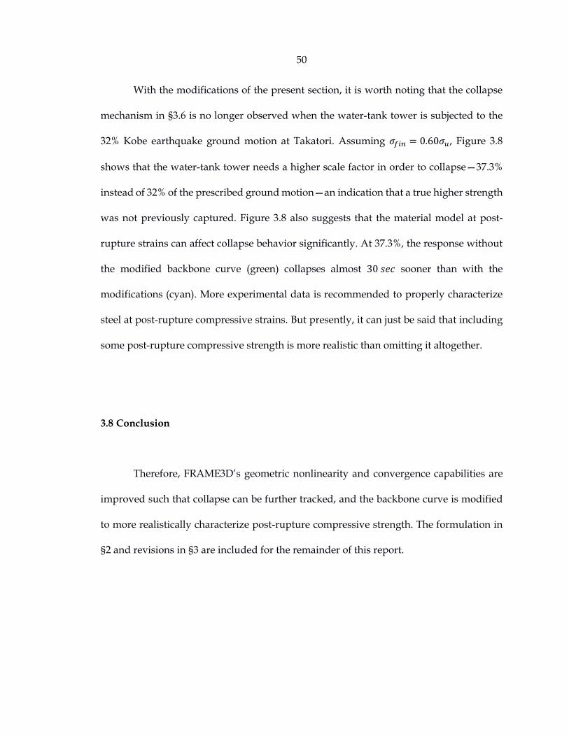
50
With the modifications of the present section, it is worth noting that the collapse
mechanism in §3.6 is no longer observed when the water-tank tower is subjected to the
32% Kobe earthquake ground motion at Takatori. Assuming 𝜎𝑓𝑖𝑛 = 0.60𝜎𝑢, Figure 3.8
shows that the water-tank tower needs a higher scale factor in order to collapse—37.3%
instead of 32% of the prescribed ground motion—an indication that a true higher strength
was not previously captured. Figure 3.8 also suggests that the material model at post-
rupture strains can affect collapse behavior significantly. At 37.3%, the response without
the modified backbone curve (green) collapses almost 30 𝑠𝑒𝑐 sooner than with the
modifications (cyan). More experimental data is recommended to properly characterize
steel at post-rupture compressive strains. But presently, it can just be said that including
some post-rupture compressive strength is more realistic than omitting it altogether.
3.8 Conclusion
Therefore, FRAME3D’s geometric nonlinearity and convergence capabilities are
improved such that collapse can be further tracked, and the backbone curve is modified
to more realistically characterize post-rupture compressive strength. The formulation in
§2 and revisions in §3 are included for the remainder of this report.
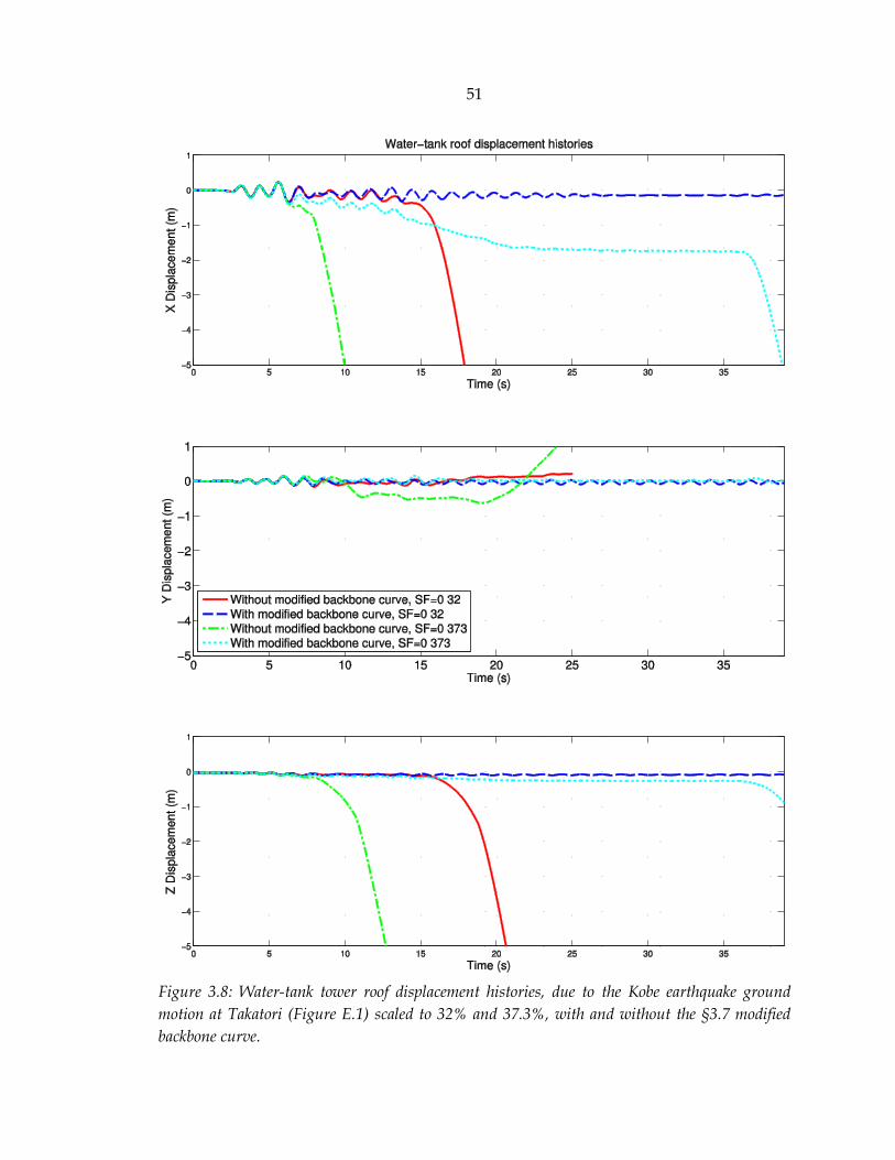
51
Figure 3.8: Water-tank tower roof displacement histories, due to the Kobe earthquake ground
motion at Takatori (Figure E.1) scaled to 32% and 37.3%, with and without the §3.7 modified
backbone curve.

52
PART II
A Computationally Efficient,
Parallel FRAME3D

53
Chapter 4
Overview of Parallel Computing
4.1 General
The revised FRAME3D at the conclusion of Part I exhibits superior convergence
capabilities compared to previous versions. The next goal of the present work is to
improve FRAME3D’s computational performance so that the nonlinear response of very
tall buildings can be computed more quickly. For example, Part I’s FRAME3D (an
unoptimized serial code) would compute the nonlinear dynamic time-history collapse of
a 60-story building (designed in §8) with a wall time (i.e., from the user’s perspective;
defined in §4.4.2) of 27 days.

54
In Part II (§§4 – 7), a computationally efficient, parallel FRAME3D (PFRAME3D)
is developed. The serial code is optimized, reducing the wall time of the same
computation to 3.5 days. Then the optimized serial code is parallelized, further reducing
the wall time to 5.7 hours (using 128 cores).
The current chapter, which presents an overview of parallel computing, is
organized as follows:
Review of parallel computing in structural engineering (§4.2)
Terminology (§4.3)
Parallel performance measures (§4.4)
Computer architecture (§4.5)
Speedup strategy (§4.6).
4.2 Review of parallel computing in structural engineering
Parallel computing for finite-element programs is becoming an increasingly
important topic due to rapidly improving computer environments. For dynamic
programs that use explicit integration, distributed-memory parallel-computing strategies
are well established. However, explicit integration is not preferred for large buildings
because stiff elements require the use of unreasonably small time steps. Additionally,
explicit dynamic analysis requires non-zero mass at every DOF in order to invert the mass
matrix in the solution phase, but building models often assume zero mass at rotational
DOFs. Thus, implicit integration schemes are usually preferred in structural engineering.

55
In the literature, there is yet to be a parallel framework intended specifically for
the analysis of very tall buildings. Industry standards like PERFORM-3D and ETABS are
currently limited to the shared-memory platform (one computer with multiple cores).
A distributed-memory (multiple computers) parallel version of OpenSees
(OpenSeesSP) (McKenna and Fenves 2007) was developed and addressed the general case
of sparse systems (uses sparse linear solvers like MUMPS, Petsc, and SuperLU). It was
reported, however, to not scale well when using implicit integration (McKenna 2012). A
bottleneck is present due to communication overhead with a “head-node.” Thus, it was
recommended to use OpenSeesSP with explicit integration, which as stated above is not
ideal for building structures.
Another distributed-memory parallel version of OpenSees (OpenSeesMP)
(McKenna and Fenves 2007) has also been developed and achieves scalability for the
naturally parallel case that is commonly used in parameter studies (i.e., many concurrent
simulations). To use OpenSeesMP, a user must write parallel scripts—and account for
potential deadlock (cyclic dependencies when message passing), race conditions (non-
determinism due to parallelization and variable CPU speeds), and load imbalances.
OpenSeesMP also allows for the analysis of a single large structure, but it requires a user
to specify subdomains. For example, a large model must be re-created if the user wants to
split up the problem differently (e.g., to use 4 computer nodes instead of 2). This
framework may not be ideal for highly complex structures.
Cho (2012) developed a parallel framework for the implicit finite-element analysis
of reinforced concrete walls. He observed scalability and his work is referenced in §B.1,
but a different framework is found to be more suitable for very tall buildings. Essentially,

56
Cho (2012) addressed the parallelization of wide-band systems, but of interest here are
narrow-band systems.
Therefore, the parallel framework developed in the current report is unique in that
it is intended for the nonlinear implicit analysis of large narrow-band systems
representing tall buildings. To the knowledge of the author, it is the first of its kind.
4.3 Terminology
The reader may not be familiar with some of the terminology used by the parallel
computing (PaC) and/or structural finite element modeling (FEM) communities. To add
confusion, word usage may overlap between these two disciplines. For example, node
refers to a computer in a computer cluster in PaC, but to a joint in a FEM model. Or, local
refers to a single node in PaC, but to the element-level calculations in FEM. And global
refers to a set of nodes in PaC, but to the structure-level calculations in FEM. §A.1 defines
terms as they are used in this paper.
4.4 Parallel performance measures
4.4.1 General
To quantify the effectiveness of parallelization, two performance measures are
defined:

57
Wall time (§4.4.2)
Speedup (§4.4.3).
4.4.2 Wall time
Perhaps the most intuitive way to assess performance is to consider wall time; the
ultimate goal of parallelization is to minimize this quantity. Wall time refers to the elapsed
time as perceived by a user. When plotted against the number of cores used, wall time can
help quantify how scalable a program is. Specifically, two notions of scalability are used:
strong-scaling and weak-scaling.
Strong-scaling involves varying the number of cores used to complete a constant
overall “workload.” This notion addresses the effectiveness of parallelization for
completing a single large computation as quickly as possible.
Weak-scaling involves simultaneously varying both the number of cores used and
the total workload such that the “workload per core” is constant. This notion addresses
the effectiveness of parallelization for completing larger computations (using more
parallelism) in the same amount of time as smaller computations (using less parallelism).
For clarity in the present discussion (to account for both notions of scalability) wall
time is written as 𝑇(𝑁,𝑊), a function of the number of cores used 𝑁, and the number of
“workload units” performed 𝑊 (e.g., if 1 “workload unit” is performed, then 𝑊 = 1; if 𝑁
“workload units” are performed, then 𝑊 = 𝑁, etc.). In a strong-scaling study, wall time is
denoted as 𝑇(𝑁,𝑊 = 1); in a weak-scaling study, it is 𝑇(𝑁,𝑊 = 𝑁).
Consider wall time vs. the number of cores used (i.e., 𝑇 vs. 𝑁). Strong-scaling is
“ideal” if 𝑇(𝑁, 1) halves when 𝑁 doubles, and “poor” if 𝑇(𝑁, 1) is constant vs. 𝑁. The latter

58
condition is typically approached as more cores are added (Amdahl 1967). Weak-scaling
is “ideal” if 𝑇(𝑁,𝑁) is constant vs. 𝑁, and “poor” if 𝑇(𝑁,𝑁) doubles when 𝑁 doubles.
(The terms “ideal” and “poor” are used for convenience. It is possible to have
“better than ideal” scaling, e.g., Cho (2012) due to favorable cache-effects, or “worse than
poor” scaling, i.e., “parallel slowdown,” due to excessive communication costs.
Nevertheless, “ideal” and “poor” serve as appropriate reference points.)
4.4.3 Speedup
Speedup, the relative wall times between serial (1-core) and parallel (𝑁-cores)
computations, is a unitless metric that measures “how much faster” a parallel program is
than its serial counterpart. It is most often defined (as is done here) in the strong-scaling
sense, or
𝑆𝑝𝑒𝑒𝑑𝑢𝑝(𝑁) =𝑇(1,1)
𝑇(𝑁,1). (Eq. 4.1)
Speedup is “ideal” if it is 1:1 proportional to 𝑁, and “poor” if it is constant vs. 𝑁. As
stated in §4.4.2, the latter condition is typically approached as more cores are added.
4.5 Computer architecture
All analyses are run using Garuda, a high-performance computer cluster at Caltech.
The cluster has 75 nodes with 8 cores per node (a core is assumed to be the basic unit that
can execute a single stream of commands); up to 600 cores may be simultaneously used
in analysis. More specifically, it has 75 Dell PowerEdge 1950s, each with 2.33 GHz dual
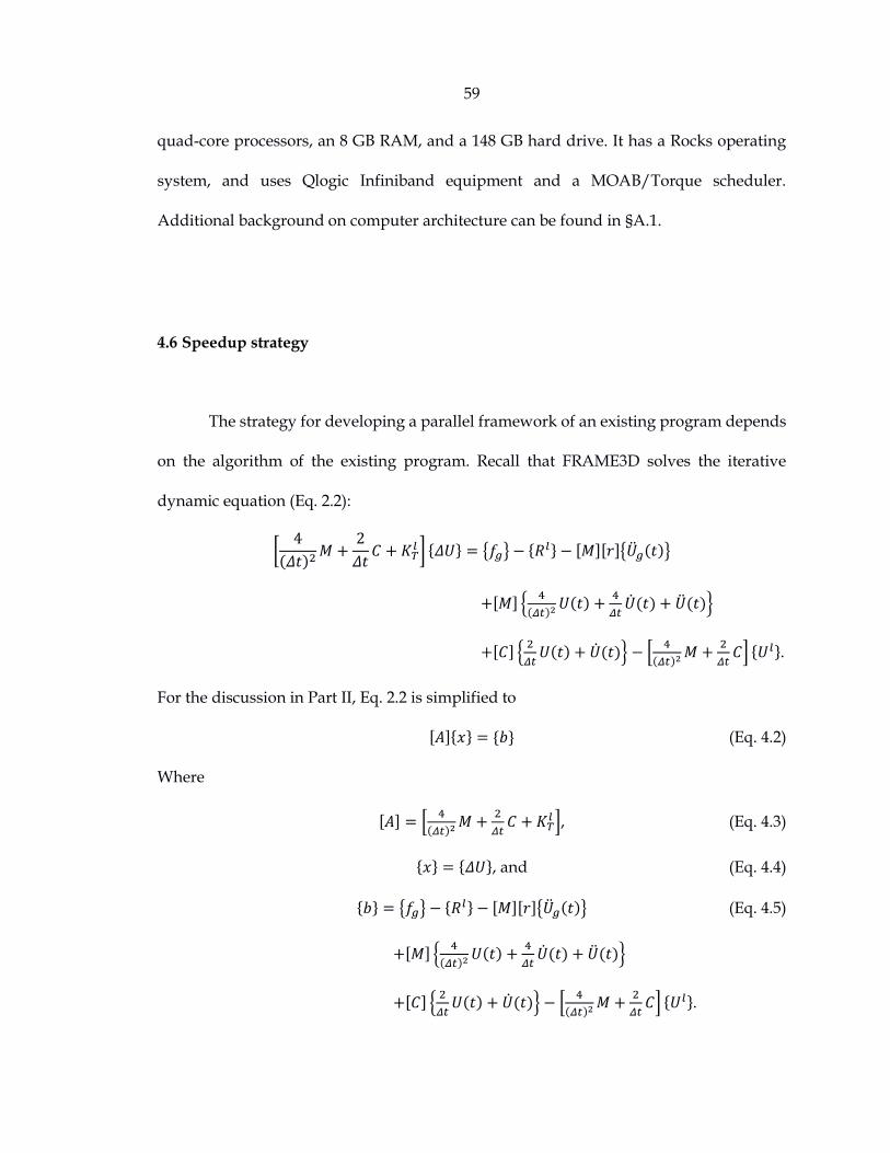
59
quad-core processors, an 8 GB RAM, and a 148 GB hard drive. It has a Rocks operating
system, and uses Qlogic Infiniband equipment and a MOAB/Torque scheduler.
Additional background on computer architecture can be found in §A.1.
4.6 Speedup strategy
The strategy for developing a parallel framework of an existing program depends
on the algorithm of the existing program. Recall that FRAME3D solves the iterative
dynamic equation (Eq. 2.2):
[4
(𝛥𝑡)2𝑀 +
2
𝛥𝑡𝐶 + 𝐾𝑇
𝑙 ] {𝛥𝑈} = {𝑓𝑔} − {𝑅𝑙} − [𝑀][𝑟]{�̈�𝑔(𝑡)}
+[𝑀] {4
(𝛥𝑡)2𝑈(𝑡) +
4
𝛥𝑡�̇�(𝑡) + �̈�(𝑡)}
+[𝐶] {2
𝛥𝑡𝑈(𝑡) + �̇�(𝑡)} − [
4
(𝛥𝑡)2𝑀+
2
𝛥𝑡𝐶] {𝑈𝑙}.
For the discussion in Part II, Eq. 2.2 is simplified to
[𝐴]{𝑥} = {𝑏} (Eq. 4.2)
Where
[𝐴] = [4
(𝛥𝑡)2𝑀+
2
𝛥𝑡𝐶 + 𝐾𝑇
𝑙 ], (Eq. 4.3)
{𝑥} = {𝛥𝑈}, and (Eq. 4.4)
{𝑏} = {𝑓𝑔} − {𝑅𝑙} − [𝑀][𝑟]{�̈�𝑔(𝑡)} (Eq. 4.5)
+[𝑀] {4
(𝛥𝑡)2𝑈(𝑡) +
4
𝛥𝑡�̇�(𝑡) + �̈�(𝑡)}
+[𝐶] {2
𝛥𝑡𝑈(𝑡) + �̇�(𝑡)} − [
4
(𝛥𝑡)2𝑀+
2
𝛥𝑡𝐶] {𝑈𝑙}.

60
Thus, the solution procedure (§2.2) simplifies to five general steps (referred to as Steps 1 –
5 in Part II). For each global iteration 𝑙:
(1) Check convergence
(2) Update* [𝐴]
(3) Solve for 𝑥 in [𝐴]{𝑥} = {𝑏}
(4) Update geometry
(5) Update {𝑏}
*Most of the work for Step 2 involves iterating locally (element-level) to determine
EF3/EF5 element tangent stiffnesses. This work is already done in Step 5 and is not
included in Step 2’s wall time.
By recording the wall time (𝑠𝑒𝑐) per simulation time step, using three example nonlinear
dynamic time-history collapse simulations (small/medium/large), it is shown in Figure
4.1 and Figure 4.2 that Steps 3 and 5 are usually the costliest—based on Part I’s FRAME3D,
an unoptimized serial code. These three systems are discussed further in §7, along with
performance results. In terms of strategy, it can be seen that as system size increases, Step
3 becomes more significant. Step 5 is significant for all sizes and cannot be ignored.
Thus, the speedup strategy here prioritizes Steps 3 and 5. §5 focuses on Step 3, and
§6 focuses on step 5. Steps 2 and 4 are similar to step 5, and therefore, are also covered in
§6. Step 1, though it uses insignificant computation time, is automatically sped up due to
the implementations of §5 and §6. As a result, every step is made parallel.
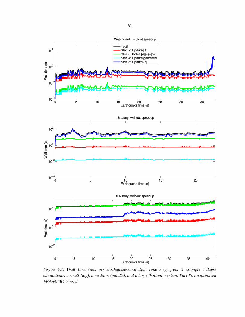
61
Figure 4.1: Wall time (sec) per earthquake-simulation time step, from 3 example collapse
simulations: a small (top), a medium (middle), and a large (bottom) system. Part I’s unoptimized
FRAME3D is used.

62
Figure 4.2: Computational cost breakdown of significant steps, from three collapse simulations.
Part I’s unoptimized FRAME3D is used.
*The 650 ℎ𝑟 (27 𝑑𝑎𝑦) simulation never actually ran. It is estimated based on: (1) the wall
time of an optimized 1-core analysis, and (2) the relative speeds of optimized and
unoptimized 1-core code.
Step 2 Step 3
Step 4
Step 5
Misc.
Water-tank tower (3.58 hrs)
Step 2
Step 3
Step 4
Step 5
Misc.
18-story building (38.6 hrs)
Step 2
Step 3
Step 4
Step 5
Misc.
60-story building (650 hrs*)
Step 2 Step 3 Step 4 Step 5 Misc.

63
Chapter 5
The Direct Solver
5.1 General
Many researchers have studied efficient solutions to the 𝑛-DOF linear equation
[𝐴]{𝑥} = {𝑏} (Step 3 in §4.6). In this chapter, various LU-type direct solvers are explored:
LU and Cholesky solvers in general (§5.1)
Row-based solver (§5.2; the original FRAME3D solver)
Column-based solver (§5.2)
Blocked solver (§§5.2-5.3)
Divide-and-conquer solver (§5.4).

64
The divide-and-conquer solver implemented with hybrid parallelism is chosen for
PFRAME3D.
The LU solution procedure, which assumes that [𝐴]{𝑥} = {𝑏} can be solved without
shifting, has two sub-steps: factorization and substitution.
(3.1) Factorization: Factor [𝐴] to an [𝐿][𝐷][𝑈] or [𝐿][𝑈] system, where [𝐿] and [𝑈]
are lower and upper triangular matrices, respectively, and [𝐷] is a diagonal
matrix. This sub-step is often written as
[𝐴] = [𝐿][𝐷][𝑈] (or [𝐿][𝑈]). (Eq. 5.1)
(3.2) Substitution: Solve the factored system [𝐿][𝐷][𝑈]{𝑥} = {𝑏} with three
equations:
[𝐿]{𝑧} = {𝑏} (Eq. 5.2)
[𝐷]{𝑦} = {𝑧} (Eq. 5.3)
[𝑈]{𝑥} = {𝑦} (Eq. 5.4)
where {𝑧} = [𝐷][𝑈]{𝑥}. Eq. 5.2 and 5.4 use forward and back substitution, respectively,
because [𝐿] and [𝑈] are triangular. Eq. 5.3 is present if the system was factored as LDU
(skipped if LU). Sub-steps 3.1 and 3.2 use about 𝑛3
3 and 𝑛2 multiplications, respectively,
for an 𝑛 × 𝑛 linear system.
For algorithmic efficiency and storage savings, symmetry and positive-
definiteness are considered. For a symmetric positive-definite [𝐴], [𝐿]𝑇 = [𝑈] and the
factored system is [𝐿][𝐷][𝐿]𝑇{𝑥} = {𝑏} (or [𝐿][𝐿]𝑇{𝑥} = {𝑏}). The resulting procedure,
called 𝐿𝐷𝐿𝑇 or 𝐿𝐿𝑇 (Cholesky) factorization, requires 𝑛3
6 multiplications—half of the LU
factorization multiplication count.

65
For a banded [𝐴], the terms outside of the band can be skipped, reducing wall time
and storage. As a result, factorization and substitution need 𝑛𝑚2
6 and 𝑛𝑚 multiplications,
respectively, where 𝑚 is the system half-bandwidth. And because [𝐴] is symmetric and
banded, storage requirements reduce from 𝑛2 to 𝑛𝑚. A tall building has a narrow-band
symmetric positive-definite [𝐴] matrix where 𝑚 is roughly the number of DOFs per story
level; e.g., for a 60-story building, 𝑚 ≈𝑛
60. Therefore, only banded Cholesky-type solvers
are considered. The above simplifications are summarized in Table 5.1.
Table 5.1: Multiplication-division count and storage for LU and Cholesky factorization.
Factorization type # Multiplications in factorization
# Multiplications in substitution
Storage
𝐿𝑈 (or 𝐿𝐷𝑈),
non-banded
𝑛3
3
𝑛2 𝑛2
Cholesky or 𝐿𝐷𝐿𝑇,
non-banded
𝑛3
6
𝑛2 𝑛2
Cholesky or 𝐿𝐷𝐿𝑇,
banded
𝑛𝑚2
6
𝑛𝑚 𝑛𝑚
The Cholesky solvers in this chapter are subjected to a series of performance tests
(solving [𝐴]{𝑥} = {𝑏} with varied system sizes 𝑛 and half-bandwidths 𝑚). Increasing the
size of a tall building usually means increasing its height. When considering increasing
building height, 𝑛 generally increases much faster than 𝑚. For example, if 1 story is added
to a tall building, 𝑚 is constant and 𝑛 increases by 𝑚. That is not to say that increases in 𝑚
are unimportant. On the contrary, taller buildings also tend to have larger footprints
(higher 𝑚, or more DOFs per story) than shorter buildings. And the factorization costs

66
depend on 𝑚2, a stronger than linear relationship. Nevertheless, the relationship between
𝑛 and 𝑚 is one where 𝑛
𝑚 approximately reflects the number of stories in a building. Thus,
to test a solver’s suitability over a range of building heights, it is reasonable to vary 𝑛 with
a constant 𝑚.
For each solver in this chapter, performance results are reported first and
algorithms explained afterwards.
5.2 Serial (1-core) solvers
This section shows that serial optimizations can significantly improve the
performance of the direct solver. Four solvers are considered:
a row-based solver (the original FRAME3D solver),
a column-based solver,
an optimized column-based solver, and
a blocked solver.
Performance tests, where 𝑛 ranges from 2500 to 160,000 with a constant 𝑚 = 1000, show
(Figure 5.1) that serial optimizations alone can make the direct solver much faster than the
original row-based solver. For example, if 𝑛 = 80,000 and 𝑚 = 1000, factorization wall
time is reduced from 753 𝑠𝑒𝑐 (row-based) to 12.9 𝑠𝑒𝑐 (blocked). These improvements are
achieved using 1 core.

67
Figure 5.1: Wall times (sec) of serial factorization, using row-based, column-based, and blocked
solvers, where m=1000. Intel MKL is used for the “optimized” solvers.
Begin with the original FRAME3D solver. It is a row-based variant of the 𝐿𝐷𝐿𝑇
solver; it uses [𝑈] instead of [𝐿], where [𝑈]𝑇 = [𝐿]. [𝐴] is stored as an 𝑛 ×𝑚 matrix (Table
5.2), and factored to [𝑈]𝑇[𝐷][𝑈] using the algorithm on the left of Table 5.3.
A column-based version of the original solver is shown on the right of Table 5.3.
Table 5.3 shows that the only difference between the row- and column-based solvers is
the switching of indices (and the renaming of mincol to minrow—but this is trivial). The
column-based solver is more efficient (~6 times faster than row-based) because it
considers cache effects (§A.2). Essentially, computer code is more efficient when data
arrangement matches the data access pattern. In a column-major language (FORTRAN),
0.1
1
10
100
1000
10000
2.5k 5k 10k 20k 40k 80k 160k
Fact
ori
zati
on
wal
l tim
e (s
ec)
System size (n)
Row-based Column-based Optimized column-based Optimized blocked

68
this means that factorization is more efficient when [𝐴] is stored as 𝑚 × 𝑛 (Table 5.3). For
similar reasons, substitution is sped up with the 𝑚 × 𝑛 arrangement.
Table 5.2: Storage schemes for a banded matrix [A], where * represents symmetry. In this example,
n=5 and m=3.
𝒏 × 𝒏 𝒏 ×𝒎 𝒎× 𝒏
[ 𝑎00 ∗ ∗
𝑎10 𝑎11 ∗ ∗𝑎20 𝑎21 𝑎22 ∗ ∗
𝑎31 𝑎32 𝑎33 ∗
𝑎42 𝑎43 𝑎44]
[ 𝑎00 𝑎10 𝑎20𝑎11 𝑎21 𝑎31𝑎22 𝑎32 𝑎42𝑎33 𝑎43𝑎44 ]
[
𝑎00 𝑎11 𝑎22 𝑎33 𝑎44𝑎10 𝑎21 𝑎32 𝑎43𝑎20 𝑎31 𝑎42
]
Table 5.3: Row- and column-based pseudocodes for the serial factorization of a banded positive-
definite matrix.
Row-based Column-based
[𝐴] is 𝑛 ×𝑚
[𝐴] = [𝑈]𝑇[𝐷][𝑈]
[𝐴] is 𝑚 × 𝑛
[𝐴] = [𝐿][𝐷][𝐿]𝑇
do i=1,n
mincol = min(m,n-i+1)
do j=2,mincol
st = A(i,j)/A(i,1)
do k=j,mincol
A(i+j-1,k-j+1) =
A(i+j-1,k-j+1) - A(i,k)*st
continue
A(i,j) = st
continue
continue
do i=1,n
minrow = min(m,n-i+1)
do j=2,minrow
st = A(j,i)/A(1,i)
do k=j,minrow
A(k-j+1,i+j-1) =
A(k-j+1,i+j-1) - A(k,i)*st
continue
A(j,i) = st
continue
continue

69
Although much of the initial wall time reduction in Figure 5.1 can be attributed to
the switch from a row- to a column-based solver, the equivalent optimized column-based
factorization from the Intel Math Kernel Library (MKL), dpbtf2, is even faster. Intel MKL
routines, designed specifically for Intel processors, include many additional optimizations
(e.g., loop unrolling, vectorization, machine-level optimizations, etc.) that make it difficult
to outperform (dpbtf2 is ~1.5 times faster than un-optimized column-based).
Wall time is further reduced by switching to a blocked solver. The blocked solver is
a generalization of the column-based solver; it factors by block columns instead of scalar
(1 × 1 block) columns (Remon, Quintana-Orti, and Quintana-Orti 2007). Figure 5.1 shows
that an optimized 1-core blocked solver is ~6 times faster than the optimized 1-core
column-based one. Although the total operation count is similar, working with blocks
reduces cache misses (Ballard et al. 2009). Used here is the Intel MKL version of the
blocked factorization, dpbtrf, where block sizes are optimized for the processors’ cache
sizes.
To understand blocked factorization, consider the matrix [𝐴], which is split into
blocks such that
[𝐴] =
[ [𝐴00] ∗ ∗
[𝐴10] [𝐴11] ∗ ∗[𝐴20] [𝐴21] [𝐴22] ∗ ∗
[𝐴31] [𝐴32] [𝐴33] ∗
[𝐴42] [𝐴43] [𝐴44]]
(Eq. 5.5)
where ∗ represents symmetry. Assume that the first block column ([𝐴𝑖0], 𝑖 ∈ 0,1,2) has
been factored already. To continue (using the next block column, [𝐴𝑖1], 𝑖 ∈ 1,2,3):
(1) Factor the diagonal block
[𝐴11] = [𝐿11][𝐿11]𝑇 (Eq. 5.6)

70
(2) Update the block column
[𝐴21](= [𝐿21]) = [𝐴21 ][𝐿11]−𝑇 (Eq. 5.7)
[𝐴31](= [𝐿31]) = [𝐴31 ][𝐿11]−𝑇 (Eq. 5.8)
(3) Update across
[𝐴22] = [𝐴22] − [𝐿21][𝐿21]𝑇 (Eq. 5.9)
[𝐴32] = [𝐴32] − [𝐿31][𝐿21]𝑇 (Eq. 5.10)
[𝐴33] = [𝐴33] − [𝐿31][𝐿31]𝑇. (Eq. 5.11)
The serial optimizations in this section are shown to significantly improve the
performance of the direct solver. Without adding computer resources (still using 1 core),
the 𝑛 = 80,000 and 𝑚 = 1000 factorization wall time is reduced from 753 𝑠𝑒𝑐 (row-based)
to 12.9 𝑠𝑒𝑐 (blocked).
Single-core optimizations are also included for the substitution step; e.g., for 𝑛 =
80,000 and 𝑚 = 1000, substitution wall time is reduced from 2.37 𝑠𝑒𝑐 (row-based) to
0.36 𝑠𝑒𝑐 (optimized Intel MKL dpbtrs).
For small systems (e.g., elastofiber elements with interior nodes, where 𝑛 ≤ 36 <
typical block size ≈ 64), the optimized column-based solver is most efficient, with
factorization and substitution about 1.6 and 1.2 times faster, respectively, than the original
row-based solver.

71
5.3 Multi-threaded blocked solver
The blocked solver from §5.2 is easily parallelized in the shared-memory context
(multiple cores in a computer node) because only matrix-matrix operations (Eq. 5.6 – 5.11)
are performed. Shared-memory parallelism is also known as multi-threading (§A.1) where
each core executes 1 thread. Figure 5.2 shows that multi-threading the blocked solver
further reduces factorization wall time, e.g., for 𝑛 = 80,000 and 𝑚 = 1000, from 12.9 𝑠𝑒𝑐
(1 core) to 3.47 𝑠𝑒𝑐 (8 cores).
Shared-memory parallelism is often efficient because there is no communication
cost; however, a maximum of 8 cores (the number of cores in 1 node) may be utilized. To
further reduce wall time (by using more than 8 cores), a distributed-memory solver must
be considered.

72
Figure 5.2: Wall times (sec) of multi-threaded blocked factorization (dpbtrf) with 1 to 8 cores. Each
curve corresponds to a different system size n with m=1000.
5.4 Divide-and-conquer solver
The divide-and-conquer solver is a distributed-memory extension of the multi-
threaded blocked solver in §5.3. Figure 5.3 shows that for large enough systems, it can
factor faster than the 8-core blocked solver. For example, with 256 cores, it factors the 𝑛 =
80,000, 𝑚 = 1000 system in 2.10 𝑠𝑒𝑐.
Figure 5.3 shows an initial “penalty,” where the 8-core blocked solver is faster than
a 16- or 32-core divide-and-conquer solver. This penalty is a result of “fill-in,” which
0
5
10
15
20
25
30
1 2 3 4 5 6 7 8
Fact
ori
zati
on
wal
l tim
e (s
ec)
Number of cores used (N)
10k 20k 40k 80k 160k
System size (n)

73
increases the overall operation count by about 4 (Cleary and Dongarra 1997). It is further
described below, as part of the discussion on the divide-and-conquer algorithm.
A weak-scaling curve (defined in §4.4) is constructed in Figure 5.3 (solid green).
This curve shows, for example, that if workload doubles from 𝑛 = 80,000 to 𝑛 = 160,000
with a constant 𝑛 = 5000 workload per 8 cores, factorization wall time increases by a
factor of about 1.22. (Recall from §4.4.2 that weak-scaling is “ideal” if this factor is 1.0 and
“poor” if it is 2.0.)
Figure 5.3: Wall times (sec) of divide-and-conquer factorization with 8 to 256 cores. Each curve
corresponds to a different system size n with m=1000. With 8 cores, the multi-threaded blocked
factorization from §5.3 is used. A weak-scaling curve (solid green) is constructed (where workload
is n = 5000 per 8 cores).
0
2
4
6
8
10
12
0 50 100 150 200 250 300
Fact
ori
zati
on
wal
l tim
e (s
ec)
Number of cores used (N)
10k 20k 40k 80k 160k Weak-scaling
System size (n)

74
Performance results for divide-and-conquer substitution (Figure 5.4) show that
“fill-in” has little effect on parallel substitution and that the weak-scaling curve is
relatively constant. For example, if workload doubles from 𝑛 = 80,000 to 𝑛 = 160,000
with a constant 𝑛 = 5000 workload per 8 cores, substitution wall time increases by a factor
of 1.17.
Figure 5.4: Wall times (sec) of divide-and-conquer substitution with 8 to 256 cores. Each curve
corresponds to a different system size n with m=1000. With 8 cores, the multi-threaded blocked
substitution from §5.3 is used. A weak-scaling curve (solid green) is constructed (where workload
is 𝑛 = 5000 per 8 cores).
0
0.1
0.2
0.3
0.4
0.5
0.6
0.7
0.8
0 50 100 150 200 250 300
Sub
stit
uti
on
wal
l tim
e (s
ec)
Number of cores used (N)
10k 20k 40k 80k 160k Weak-scaling
System size (n)
75
The divide-and-conquer solver is designed for narrow-band systems, or 𝑚 ≪ 𝑛
(Cleary and Dongarra 1997). [𝐴] is divided into “large blocks” (1 block per process), as
shown in Figure 5.5 and Figure 5.6, where each block is (mostly) factored locally and
independently. ([𝐴] is in symmetric band form 𝑚 × 𝑛, locally stored in 𝑝 processes as 𝑚 ×
𝑛𝑏, where 𝑛𝑏 ≈𝑛
𝑝. Here, 𝑝 also equals the number of “large blocks” used.) A permutation
matrix [𝑃], which depends on 𝑛, 𝑚, and 𝑝, determines how [𝐴] is uncoupled. To solve the
linear equation:
(1) Left multiply [𝐴]{𝑥} = {𝑏} with [𝑃] to get
[𝑃][𝐴]([𝑃]𝑇[𝑃]){𝑥} = [𝑃]{𝑏} (Eq. 5.12)
(2) Factor
[𝑃][𝐴][𝑃]𝑇 = [𝐿][𝐿]𝑇 (Eq. 5.13)
(3) Solve
[𝐿][𝐿]𝑇{�̂�} = {�̂�} (Eq. 5.14)
where {�̂�} = [𝑃]{𝑥} and {�̂�} = [𝑃]{𝑏},
(4) Recover
{𝑥} = [𝑃]𝑇{𝑥}. (Eq. 5.15)
The permuted [𝐴] matrix is stored locally (e.g., as shown in Figure 5.7). Each local matrix
is factored independently (e.g., to Figure 5.8) using
[𝐴𝑖] = [𝐿𝑖][𝐿𝑖]𝑇 (Eq. 5.16)
[𝐿𝑖][𝐵𝑖′]𝑇 = [𝐵𝑖]
𝑇 (Eq. 5.17)
[𝐶𝑖′] = [𝐶𝑖] − [𝐵𝑖
′][𝐵𝑖]𝑇 (Eq. 5.18)
[𝐿𝑖][𝐺𝑖]𝑇 = [𝐷𝑖] (Eq. 5.19)
[𝐸𝑖] = [𝐺𝑖][𝐺𝑖]𝑇 (Eq. 5.20)

76
[𝐹𝑖] = [𝐵𝑖′][𝐻𝑖]
𝑇 (Eq. 5.21)
where [𝐻𝑖] are the last 𝑚 columns of [𝐺𝑖]. At this point, it is worth noting that the
“interface” blocks ([𝐸𝑖], [𝐹𝑖], and [𝐶𝑖′]) are not completely factored yet. Figure 5.9 shows
that, as the final step in divide-and-conquer factorization, these “interface” blocks are
combined as a tridiagonal block system and factored. The local storage of the factored
permuted matrix is shown in Figure 5.10, ready for substitution.
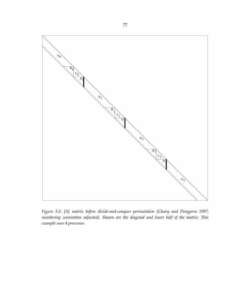
77
Figure 5.5: [A] matrix before divide-and-conquer permutation (Cleary and Dongarra 1997,
numbering convention adjusted). Shown are the diagonal and lower half of the matrix. This
example uses 4 processes.

78
Figure 5.6: [A] matrix after divide-and-conquer permutation (Cleary and Dongarra 1997,
numbering convention adjusted). Shown are the diagonal and lower half of the permuted matrix.
This example uses 4 processes.

79
Figure 5.7: Local storage of process 2 after divide-and-conquer permutation, before factorization
(Cleary and Dongarra 1997). Only the diagonal and lower half of the matrix are stored.
Figure 5.8: Local storage of process 2 after the independent portion of factorization (Cleary and
Dongarra 1997). Only the diagonal and lower half of the matrix are stored.

80
Figure 5.9: Final step for the factorization of the “interface” blocks combined as a tridiagonal block
system. Shown are the diagonal and lower half of the matrix. This example shows 3 interfaces (4
processes are assumed).
Figure 5.10: Local storage of process 2 at the end of factorization (Cleary and Dongarra 1997,
edited). Only the diagonal and lower half of the matrix are stored.

81
[𝐴] can be divided successfully only if 2(𝑚 − 1) ≤ 𝑛𝑏 . In other words, 𝑝 has the
upper limit
𝑝 ≤𝑛
2(𝑚−1) (Eq. 5.22)
after which additional parallelization is not possible. For example, if 𝑛 = 40,000 and 𝑚 =
1000, [𝐴] may be split into a maximum of 20 local blocks. So as to not limit the divide-
and-conquer solver to (for this example) 20 cores, a hybrid-parallel implementation is
used, where
𝑝 is the number of computer nodes used (1 process per computer node), and
the local operations (e.g., Eq. 5.16 – 5.21) are performed in parallel (8 cores per
process).
Thus for the current example, up to 160 cores may be used. It is worth noting, however,
that for a fixed problem size, as 𝑝 is increased to approach the limit set by Eq. 5.22, the
divide-and-conquer solver becomes less efficient. This is due to the increasing cost to
factor the “interface” blocks (as 𝑝 is increased, there are overall more “interface” blocks)
relative to cost of performing the independent calculations of Eq. 5.16 – 5.21. Fortunately,
if problem size is assumed to grow with 𝑛, more cores may be used for larger problems
(e.g., 320 cores if 𝑛 = 80,000 and 𝑚 = 1000, etc.).
The primary drawback of the divide-and-conquer solver is “fill-in.” Due to the
permutation, matrices [𝐸𝑖], [𝐹𝑖], and [𝐺𝑖] must also be factored, increasing the overall
operation count to about 4 times greater than sequential Cholesky factorization (Cleary
and Dongarra 1997). This effect is observable in Figure 5.3, where the divide-and-conquer
solver is slower than the 1-process (8-core) blocked solver if 4 processes (32 cores) or less
are used.

82
But for increasing 𝑛 with constant 𝑚, the operation count per process can be
bounded. Each process operates on its own local matrix (e.g., Figure 5.8), which is 𝑛𝑏 ×
𝑛𝑏. Eq. 5.16, computed by the multi-threaded blocked factorization from §5.3, operates on
a band matrix of size 𝑚 × (𝑛𝑏 − 2𝑚). Eq. 5.17, 5.18, 5.19, and 5.21 operate on 𝑚×𝑚
matrices. And Eq. 5.19 and 5.20 operate on matrices smaller than 𝑚× 𝑛𝑏. Increasing 𝑝
reduces 𝑛𝑏, so as long as 𝑚 is constant, the per-process operation counts for Eq. 5.16 – 5.21
can be bounded. Additionally, it can be seen from Figure 5.9 that the cost to finish
factoring the “interface” blocks is a function of 𝑚 and 𝑝. Finally, because the factored
permuted system is stored locally, substitution can be done independently with costs
related to 𝑛𝑏 and 𝑚. In other words, the cost of the divide-and-conquer algorithm is
bounded by a function of 𝑛𝑏, 𝑚, and 𝑝—not 𝑛 directly.
Communication, which occurs three times, has a cost that is bounded by a function
of 𝑚. First, at the initial permutation, each process gives [𝐷𝑖]𝑇, an 𝑚 ×𝑚 matrix, to its
neighbor. Second, in order to finish factoring the “interface” blocks, each process gives
[𝐶𝑖′], an 𝑚 ×𝑚 matrix, to its neighbor. Third, before substitution begins, each process gives
a 2𝑚 × 1 vector to its neighbor. These communication costs are independent of 𝑛.
Finally, the divide-and-conquer solver has a major advantage that is more
thoroughly discussed in the next chapter: preparation and communication costs are low
when inserted into the context of PFRAME3D’s global iterations. Other distributed-
memory solvers, such as the Cho (2012) parallel pipelined solver (§B.1) are considered,
too, but the divide-and-conquer approach is found to be more suitable for large narrow-
band systems.

83
5.5 Conclusion
In this chapter, several Cholesky direct solvers are considered and one is chosen
for PFRAME3D. First, serial optimizations are shown to be significant, e.g., for the 𝑛 =
80,000 and 𝑚 = 1000 system, factorization wall time is reduced from 753 𝑠𝑒𝑐 (row-based)
to 12.9 𝑠𝑒𝑐 (1-core blocked, §5.2). Next, shared-memory parallelization is shown to further
reduce wall time of the same computation to 3.47 𝑠𝑒𝑐 (8-core blocked, §5.3). Finally,
distributed-memory parallelization is shown to reduce it even further to 2.10 𝑠𝑒𝑐 (divide-
and-conquer with 256 cores, §5.4).
Recall (§4.6) that the 60-story building dynamic time-history collapse simulation,
with 𝑛 = 30,606, 𝑚 = 514, would take 650 hrs (27 days) to complete if run with Part I’s
unoptimized FRAME3D. Recall also that the row-based direct solver would use about
89% of those 27 days. If serial optimizations are applied to the direct solver, the overall 1-
core simulation would take only 83.6 hrs (3.5 days). Out of the 83.6 hrs, 14.2 hrs are spent
in the optimized 1-core direct solver. Parallelization of the direct solver reduces the 14.2
hrs (1-core blocked) to 3.74 hrs (128-core divide-and-conquer).
In other words, the direct solver is no longer the most time-consuming part of the
overall simulation. 69.4 hrs (i.e., 83.6 hrs minus 14.2 hrs) are spent outside of the direct
solver. Therefore, the next challenge is to speed up the rest of FRAME3D. This is the topic
of §6.

84
Chapter 6
Domain Decomposition
and Parallel Updating
6.1 General
So far, Step 3 in §4.6 is sped up. §6, which focuses on the remaining steps, is
organized as follows:
Domain decomposition (§6.2)
Parallel updating of {𝑏}𝑖 (§6.3; Step 5 in §4.6)
Parallel updating of [𝐴]𝑖 (§6.4; Step 2 in §4.6)

85
Parallel geometric updating (§6.5; Step 4 in §4.6)
Parallel convergence check (§6.6; Step 1 in §4.6)
Parallel input-output (§6.7)
Miscellaneous considerations (§6.8).
The result of this chapter is an efficient hybrid-parallel FRAME3D.
For clarity in this chapter, the term node is used in the finite-element sense, a joint
in the structural model. The parallel-computing node is referred to as a process to avoid
confusion. (A process is a single instance of a computer program being run. In a typical
hybrid-parallel program, each computer node in a computer cluster starts a process. See
§A.1 for more on terminology usage.)
6.2 Domain decomposition
6.2.1 General
This section shows how domain decomposition—the splitting up of a structural
model across processes as shown in Figure 6.1—is implemented in PFRAME3D. The
primary reason to conduct domain decomposition is to address the fact that a single
computer may not have enough RAM to hold all of the nodal, element, fiber, hysteretic,
etc. data of a very large model. Fortunately in the distributed-memory context, domain
decomposition can bound the per-process (i.e., per-computer) storage requirements. Even
if this RAM limit is not reached, domain decomposition still provides a more efficient use

86
of computing resources because parallelization eliminates the need for a given process to
access the entire data set (describing the structural model).
Figure 6.1: Domain decomposition of a structure.
Previous parallel implicit programs address domain decomposition in two parts:
one scheme for element-state updates, and another for the equation solver. OpenSeesSP
and the Cho (2012) parallel program approach domain decomposition in this manner.
This approach, however, results in additional “preparation” costs. For example, Cho
(2012) noted that 𝑛 communication steps are needed to transition from the element-state

87
updates to the parallel-pipelined solver. He showed that these costs are asymptotically
negligible for wide-band systems (as 𝑛 and 𝑚 → ∞, compared to the overall factorization
costs). But for narrow-band systems, which are of interest in the present work, these costs
are non-negligible.
A “unified” approach is developed for PFRAME3D. Domain decomposition is
most effective when inter-process communication is minimized between subroutines, e.g.,
between element-state updates and the direct solver of an implicit program. The
“preparation” costs noted in Cho (2012) are a non-issue for parallel explicit programs
because there is no linear equation solver in the explicit algorithm. The extent of
communication in explicit programs is between “nearest neighbors.” That is, a process
communicates only data from the boundary of its subdomain to the neighboring process
that shares the same boundary. This paradigm, which is well suited for parallel
computing, is applied to PFRAME3D, an implicit program. Domain decomposition is
implemented such that, between the element-state updates and the global solver,
processes need only to communicate 𝑚 × 1 vectors (the boundary) to their nearest
neighbors. Essentially, the domain decomposition scheme for the element-state updates
is made to match that of the divide-and-conquer solver. This “unified” domain
decomposition scheme results in the “nearest neighbor” communication pattern that is
rarely accomplished in parallel implicit programs, making PFRAME3D unique. It is
achieved in three parts:
DOF allocation (§6.2.2)
Element allocation (§6.2.3)
Node allocation (§6.2.4).

88
Additional notes on domain decomposition are presented in §6.2.5. The “DOF” data set is
distinct from the “node” data set in the following way: the “DOF” data set refers to any
global array that is stored in either 𝑚 × 𝑛 or 𝑛 × 1 form, e.g., [𝐴], {𝑥}, and {𝑏}, whereas the
“node” data set contains the coordinates, dimensions, deformation, etc. of every building
joint.
6.2.2 DOF allocation
Start with the fact that the divide-and-conquer solver uncouples the DOFs in [𝐴]
as shown in Figure 5.6. Before this permutation, [𝐴] is represented as an 𝑚 × 𝑛 band
(Figure 5.5), and process 𝑖 ∈ [0, 𝑝 − 1] ⊂ ℤ gets a non-overlapping 𝑚 × 𝑛𝑖 block of [𝐴]—
where 𝑚 is the half-bandwidth, 𝑛 is the total number of DOFs, 𝑝 is the number of processes
used, and 𝑛𝑖 is the number of DOFs assigned to a process 𝑖 as defined by Eq. 6.1 – 6.2. For
process 𝑖 ≠ 𝑝 − 1,
𝑛𝑖 = 𝑛𝑏 = {int (
𝑛
𝑝) , if mod (
𝑛
𝑝) = 0
int (𝑛
𝑝) + 1 , if mod(
𝑛
𝑝) ≠ 0
(Eq. 6.1)
where 𝑛𝑏 is the standard block size. For process 𝑖 = 𝑝 − 1,
𝑛𝑝−1 = 𝑛 − (𝑝 − 1)𝑛𝑏 ≤ 𝑛𝑏. (Eq. 6.2)
Denote process 𝑖’s block as [𝐴]𝑖. ([𝐴]𝑖 is different from [𝐴𝑖] in Figure 5.5 to Figure 5.7; the
former refers to the entire local block, while the latter refers to a sub-block and is irrelevant
in the present chapter.)
The divide-and-conquer solver also requires that {𝑥} and {𝑏} be split up. To use it,
process 𝑖 gets an 𝑛𝑖 × 1 portion of both vectors, denoted {𝑥}𝑖 and {𝑏}𝑖.

89
Other 𝑚 × 𝑛 and 𝑛 × 1 arrays are split similarly—into 𝑚× 𝑛𝑖 and 𝑛𝑖 × 1 blocks,
respectively. Recall (§4.6) that [𝐴]{𝑥} = {𝑏}, is simplified from the dynamic equation of
motion. Thus, process 𝑖 gets a non-overlapping block from [𝑀], [𝐶], [𝐾𝑇𝑙 ], {𝛥𝑈}, {𝑓𝑔}, {𝑅
𝑙},
[𝑟], {𝑈(𝑡)}, and {𝑈𝑙}, denoted [𝑀]𝑖, [𝐶]𝑖, [𝐾𝑇𝑙 ]𝑖, {𝛥𝑈}𝑖, {𝑓𝑔}𝑖
, {𝑅𝑙}𝑖, [𝑟]𝑖, {𝑈(𝑡)}𝑖, and {𝑈𝑙}𝑖.
Process 𝑖 also gets [𝐾]𝑖𝑝𝑠
, a non-overlapping block from [𝐾]𝑝𝑠, the global stiffness matrix
due to PS elements (§2.7). No process ever has a complete global copy of any of the above
arrays.
6.2.3 Element allocation
Recall (§2.2) that [𝐾𝑇𝑙 ] & {𝑅𝑙} are assembled from beam, PZ, diaphragm, and/or
spring elements. In parallel, process 𝑖 assembles [𝐾𝑇𝑙 ]𝑖 & {𝑅𝑙}𝑖 only. Thus it needs only the
set of elements that contribute to at least 1 DOF of [𝐾𝑇𝑙 ]𝑖 & {𝑅𝑙}𝑖, denoted ℰ𝑖 ⊂ ℰ, where ℰ
is the set of elements in the entire model. If an element contributes to [𝐾𝑇𝑙 ]𝑖 & {𝑅𝑙}𝑖 and
[𝐾𝑇𝑙 ]𝑖+1
& {𝑅𝑙}𝑖+1, it belongs to both ℰ𝑖 and ℰ𝑖+1; multiple copies are allowed because the
element-level calculations are deterministic. As shown in Figure 6.2, element subdomains
can overlap by up to 1 story worth of elements. The percent of overlap is smaller for taller
buildings.

90
Figure 6.2: Two-dimensional example illustrating element and node subdomain overlap. The solid
lines represent beam elements and the dots represent nodes. The dashed line marks the division
between the non-overlapping DOF subdomains of processes i and i+1. The highlighted (grey)
elements and nodes belong to both processes 𝑖 and 𝑖 + 1, i.e., are overlapping.
6.2.4 Node allocation
Recall (§§2.3 – 2.8) that the element-level calculations depend on the incremented
displacements of the global nodes. To perform a local-level beam calculation, the
positions/rotations of the beam’s two end nodes—which are based on the coordinates
and deformations of attached PZs—must be known. Similarly, a PZ calculation accesses
data from one node, a PS calculation from four nodes, and a spring calculation from one
node. Process 𝑖 needs only the set of nodes necessary for the calculation of at least one
element in ℰ𝑖, denoted 𝒩𝑖 ⊂ 𝒩, where 𝒩 is the set of nodes in the entire model. If a node
is necessary for the calculation of both an element in ℰ𝑖 and an element in ℰ𝑖+1, it belongs
ℰ𝑖+1, 𝒩𝑖+1
ℰ𝑖, 𝒩𝑖

91
to both 𝒩𝑖 and 𝒩𝑖+1. As shown in Figure 6.2, node subdomains can overlap by up to two
floors worth of nodes. The percent of overlap is small for taller buildings.
6.2.5 Additional notes
The DOF, element, and node domain decomposition happens at the start of
PFRAME3D, before analysis. Each process reads the same user-input files, skips irrelevant
data, and saves relevant data. The more levels a building has, the more it can be split up.
It is shown in §§6.3 – 6.8 that up to 𝑚-sized vectors are communicated (because of
non-overlapping DOF subdomains). Element and node data, on the other hand, are never
communicated.
The domain-decomposition scheme here allows for hybrid-parallel computations.
Process 𝑖 computes its subdomain 𝑖 in parallel using multiple cores. There is no core-to-
core communication in this shared-memory parallel layer. This approach is often superior
to a pure Message Passing Interface (MPI) scheme, where each core has its own
subdomain, requiring core-to-core communication within a computer.
6.3 Parallel updating of {𝒃}
6.3.1 General
This section shows how {𝑏} is updated in parallel (Step 5 in §4.6). Updating {𝑏}
(Step 5 in §4.6, which also includes most of the work for updating [𝐴]; see note for Step 2
in §4.6) is the most computationally expensive step outside of the direct solver. Recall

92
(§5.6) that for the optimized 1-core 60-story collapse simulation, 69.4 hrs (out of 83.6 hrs)
are spent outside of the direct solver. Updating {𝑏} uses 56.1 hrs of the 69.4 hrs. Table 6.1
shows that the parallelization of the {𝑏} calculation results in a significant reduction in
wall time and high speedups (vs. 1 core).
Recall (Eq. 4.5) that
{𝑏} = {𝑓𝑔} − {𝑅𝑙} − [𝑀][𝑟]{�̈�𝑔(𝑡)} + [𝑀] {4
(𝛥𝑡)2𝑈(𝑡) +
4
𝛥𝑡�̇�(𝑡) + �̈�(𝑡)}
+ [𝐶] {2
𝛥𝑡𝑈(𝑡) + �̇�(𝑡)} − [
4
(𝛥𝑡)2𝑀 +
2
𝛥𝑡𝐶] {𝑈𝑙}
and that process 𝑖 updates {𝑏}𝑖 only (§6.2). Thus,
{𝑏}𝑖 = {𝑓𝑔}𝑖− {𝑅𝑙}𝑖 − ([𝑀][𝑟]{�̈�𝑔(𝑡)})𝑖
+ ([𝑀] {4
(𝛥𝑡)2𝑈(𝑡) +
4
𝛥𝑡�̇�(𝑡) + �̈�(𝑡)})
𝑖
+([𝐶] {2
𝛥𝑡𝑈(𝑡) + �̇�(𝑡)})
𝑖− ([
4
(𝛥𝑡)2𝑀 +
2
𝛥𝑡𝐶] {𝑈𝑙})
𝑖. (Eq. 6.3)
The following subsections describe how each term in {𝑏}𝑖 is updated with a shared-
memory parallel layer. The discussion is organized by descending computational cost:
Parallel updating of {𝑅𝑙}𝑖 (§6.3.2)
Parallel updating of ([4
(𝛥𝑡)2𝑀+
2
𝛥𝑡𝐶] {𝑈𝑙})
𝑖 (§6.3.3)
Parallel updating of other terms in {𝑏}𝑖 (§6.3.4)
Additional notes (§6.3.5).

93
Table 6.1: Wall time and speedup of parallel {b} calculation, from 60-story dynamic time-history
collapse simulation.
Number of
cores used
Wall time
(𝒉𝒓𝒔)
Speedup
vs. 1-core
1
2
4
8
16
32
64
128
56.1
32.5
19.9
12.7
5.01
2.84
1.78
1.28
1.00
1.73
2.81
4.43
11.2
19.8
31.5
43.9
6.3.2 Parallel updating of {𝑹𝒍}𝒊
The most costly term in {𝑏}𝑖 is {𝑅𝑙}𝑖. For the same 1-core 60-story simulation, it
uses about 99% of the {𝑏}𝑖 calculation. {𝑅𝑙}𝑖 is summed from the internal forces of every
element in ℰ𝑖. Let ℰ𝑖 = ℰ𝑖𝑏 + ℰ𝑖
𝑝𝑧+ ℰ𝑖
𝑝𝑠+ ℰ𝑖
𝑠, the sets of beam, panel-zone, plane-stress, and
spring elements, respectively, in ℰ𝑖. The summation is handled in parts, based on element
type; i.e., there is a different summation loop for each set ℰ𝑖𝑏, ℰ𝑖
𝑝𝑧, ℰ𝑖
𝑝𝑠, and ℰ𝑖
𝑠 (called beam
loop, panel-zone loop, etc.).
Beam elements
Consider the contribution of beam elements ℰ𝑖𝑏 on {𝑅𝑙}𝑖. (A “beam element” is a
beam, column, or brace in a structural model.) For efficiency, the beam loop is multi-
threaded with 1 thread per core. Three types of load-balancing are considered: (1) static,

94
(2) dynamic, and (3) sorted dynamic. To understand how each type works, let 𝑐 be the
number of cores used by a process (e.g., 𝑐 = 8 in the present cluster) and let each core be
identified by 𝑗 (an integer from [0, 𝑐 − 1]). The set of beam elements that core 𝑗 calculates
for {𝑅𝑙}𝑖 is ℰ𝑖,𝑗𝑏 ⊂ ℰ𝑖
𝑏.
In static load-balancing, beam elements are evenly distributed among cores when
the beam loop begins; i.e., ℰ𝑖,𝑗𝑏 is predetermined such that |ℰ𝑖,𝑗
𝑏 | ≈|ℰ𝑖
𝑏|
𝑐, ∀𝑗. (| ∗ | is the
number of elements in set ∗.) Static load-balancing implies that ℰ𝑖,𝑗𝑏 is generally constant
for the entire simulation. Its overhead is cheaper than dynamic load-balancing, but
computations may be highly imbalanced.
Due to nonlinearity, internal forces may be calculated quickly for some beam
elements, but slowly for other beam elements. Denote the former as a fast element and the
latter as a slow element; e.g., a PH element with elastic deformations is a fast element, and
an EF3 or EF5 element with highly nonlinear deformations is likely a slow element. The
solution procedures of EF elements are iterative (§§2.4 – 2.5), so it is possible for 1 slow
element to have the same computational cost as hundreds or thousands of fast elements.
Thus, dynamic-load balancing is considered.
In dynamic load-balancing, elements are added gradually to ℰ𝑖,𝑗𝑏 during the beam
loop itself. For global iteration 𝑙, when the beam loop begins, only 1 (or a few) beam
elements are in ℰ𝑖,𝑗𝑏 ; i.e., |ℰ𝑖,𝑗
𝑏 | = 1. Beam elements are added to ℰ𝑖,𝑗𝑏 whenever every
element in ℰ𝑖,𝑗𝑏 has contributed to {𝑅𝑙}𝑖. (In PFRAME3D, beam elements are added one at
a time.) The procedure continues until every element in ℰ𝑖𝑏 has contributed to {𝑅𝑙}𝑖; i.e.,

95
∑ ℰ𝑖,𝑗𝑏𝑐−1
𝑗=0 = ℰ𝑖𝑏. The ℰ𝑖,𝑗
𝑏 when the beam loop finishes is likely different from one global
iteration to the next.
To improve dynamic load-balancing, the beam elements in ℰ𝑖,𝑗𝑏 are sorted from
slowest to fastest using the Intel MKL dlasrt routine every few global iterations or time
steps. (In PFRAME3D, the beam elements are re-sorted every time step and every 10th
consecutive unconverged global iteration.) The slowest elements are computed first, and
the fastest elements last. For the 60-story simulation with 128 cores, the {𝑏} calculation
takes 1.55 hrs with static load-balancing, and 1.28 hrs with sorted dynamic load-balancing.
15 sec were spent sorting the elements. It is possible to study the optimum re-sort
frequency, but this is not done here.
Panel-zone elements
Next, consider the contribution of panel-zone elements ℰ𝑖𝑝𝑧
on {𝑅𝑙}𝑖. Like the beam
loop, the PZ loop is multi-threaded, where core 𝑗 computes the contributions of ℰ𝑖,𝑗𝑝𝑧⊂ ℰ𝑖
𝑝𝑧
to {𝑅𝑙}𝑖. But unlike the beam loop, all PZ calculations are direct (non-iterative). Thus, static
load-balancing is implemented.
Plane-stress elements
Next, consider the contribution of plane-stress elements ℰ𝑖𝑝𝑠
on {𝑅𝑙}𝑖. Recall (§2.7)
that [𝐾]𝑝𝑠, the global stiffness matrix due to PS elements, is computed only once, before
analysis begins. The internal force vector due to PS elements is
{𝑅𝑙}𝑝𝑠 = [𝐾]𝑝𝑠{𝑈𝑙}. (Eq. 6.4)
The goal of process 𝑖 is to compute {𝑅𝑙}𝑖𝑝𝑠
.

96
To get {𝑅𝑙}𝑖𝑝𝑠
, a hybrid-parallel matrix-vector operation (using a banded symmetric
matrix) is created here because it is not found to exist in parallel linear-algebra libraries
such as ScaLAPACK. Performance results (Figure 6.3) of this hybrid-parallel operation
suggest nearly “ideal” weak-scaling (as defined in §4.4). For example, if workload doubles
from 𝑛 = 80,000 to 𝑛 = 160,000 with a constant 𝑛 = 10,000 workload per 8 cores, the
matrix-vector operation’s wall time increases by about 1%.
Figure 6.3: Wall times (sec) of matrix-vector multiplication with 8 to 128 cores. Each curve
corresponds to a different system size n with m=1000. With 8 cores, the multi-threaded matrix-
vector routine from Intel MKL (dsbmv) is used. A weak-scaling curve (solid green) is constructed
(where workload is 𝑛 = 10,000 per 8 cores).
0
0.05
0.1
0.15
0.2
0.25
0.3
0.35
0.4
0 20 40 60 80 100 120 140
Mat
rix-
vect
or
mu
ltip
licat
ion
wal
l tim
e (s
ec)
Number of cores used (N)
10k 20k 40k 80k 160k Weak-scaling
System size (n)

97
To understand the parallel matrix-vector operation, recall (§6.2) that process 𝑖 has
[𝐾]𝑖𝑝𝑠
and {𝑈𝑙}𝑖. However,
{𝑅𝑙}𝑖𝑝𝑠= ([𝐾]𝑝𝑠{𝑈𝑙})
𝑖≠ [𝐾]𝑖
𝑝𝑠{𝑈𝑙}𝑖 (Eq. 6.5)
because {𝑅𝑙}𝑖𝑝𝑠
depends on some terms in {𝑈𝑙} that are not in {𝑈𝑙}𝑖. Rather, if [𝐾]𝑝𝑠 is
decomposed into
[𝐾]𝑝𝑠 = [𝐾]𝑝𝑠1 + [𝐾]𝑝𝑠2 (Eq. 6.6)
as shown in Figure 6.4, where the white portion of the band belongs to [𝐾]𝑝𝑠1 and the grey
portion of the band belongs to [𝐾]𝑝𝑠2, a large portion of the computation can be done
independently. For process 𝑖, Eq. 6.4 becomes
{𝑅𝑙}𝑖𝑝𝑠= ([𝐾]𝑝𝑠1{𝑈𝑙})
𝑖+ ([𝐾]𝑝𝑠2{𝑈𝑙})
𝑖. (Eq. 6.7)
The first term in Eq. 6.7 can be computed without communication using the multi-
threaded Intel MKL routine dsbmv (double-precision symmetric band matrix-vector
operation) because
([𝐾]𝑝𝑠1{𝑈𝑙})𝑖= [𝐾]𝑖
𝑝𝑠1{𝑈𝑙}𝑖. (Eq. 6.8)
To compute ([𝐾]𝑝𝑠2{𝑈𝑙})𝑖, process 𝑖 gets 𝑚 − 1 terms from processes 𝑖 − 1 and 𝑖 + 1.
Communication is handled in two steps:
process 0{𝑅∗
𝑙}0
𝑙𝑎𝑠𝑡
→ …{𝑅∗
𝑙}𝑖−1
𝑙𝑎𝑠𝑡
→ process 𝑖{𝑅∗
𝑙}𝑖
𝑙𝑎𝑠𝑡
→ …{𝑅∗
𝑙}𝑝−2
𝑙𝑎𝑠𝑡
→ process (𝑝 − 1)
process 0{𝑈𝑙}
1
𝑓𝑖𝑟𝑠𝑡
← …{𝑈𝑙}
𝑖
𝑓𝑖𝑟𝑠𝑡
← process 𝑖{𝑈𝑙}
𝑖+1
𝑓𝑖𝑟𝑠𝑡
← …{𝑈𝑙}
𝑝−1
𝑓𝑖𝑟𝑠𝑡
← process (𝑝 − 1).
The superscripts indicate that only the last or first 𝑚 − 1 terms are passed, and the {𝑅∗𝑙}𝑖𝑙𝑎𝑠𝑡
indicates that {𝑈𝑙}𝑖𝑙𝑎𝑠𝑡 is pre-multiplied to avoid passing terms from [𝐾]𝑖
𝑝𝑠2.
To avoid deadlock due to cyclic dependency (i.e., some processes must send first
while others must receive first), each step is a single send-receive operation and MPI assures

98
stability internally. It can be seen that each step can be done in parallel, and that processes
communicate with their “nearest neighbor” only; thus, the cost of the communication
algorithm depends on 𝑚, not 𝑛 or 𝑝. Additionally, the first term in Eq. 6.7 is more
significant for narrow-band systems (e.g., very tall buildings), making it suited for
PFRAME3D. A pseudocode for the hybrid-parallel matrix-vector operation can be found
in §B.2.
Spring elements
Finally, consider the contribution of spring elements ℰ𝑖𝑠 on {𝑅𝑙}𝑖. The typical
number of spring elements does not require a multi-threaded spring loop.
6.3.3 Parallel updating of ([𝟒
(𝜟𝒕)𝟐𝑴+
𝟐
𝜟𝒕𝑪] {𝑼𝒍})
𝒊
Like {𝑅𝑙}𝑖, ([4
(𝛥𝑡)2𝑀 +
2
𝛥𝑡𝐶] {𝑈𝑙})
𝑖 is also updated in every global iteration. The
update of {𝑈𝑙}, covered in §6.5, is known prior to the update of {𝑏}. Because process 𝑖 has
[𝑀]𝑖, [𝐶]𝑖, and {𝑈𝑙}𝑖, ([4
(𝛥𝑡)2𝑀+
2
𝛥𝑡𝐶] {𝑈𝑙})
𝑖 is calculated using the same hybrid matrix-
vector operation in §6.2 (for the ℰ𝑖𝑝𝑠
contributions to {𝑅𝑙}𝑖; pseudocode in §B.2).

99
Figure 6.4: [𝐾]𝑝𝑠 decomposition for hybrid-parallel matrix-vector operation. The thick black lines
mark the subdomain divisions. The white portion of the band belongs to [𝐾]𝑝𝑠1 and the grey portion
of the band belongs to [𝐾]𝑝𝑠2. Shown are the diagonal and lower half of the matrix. The example
uses 4 processes.

100
6.3.4 Parallel updating of other terms in {𝒃}𝒊
{𝑈(𝑡)}𝑖 and its time derivatives are updated at the start of each time step based on
the converged {𝑈𝑙}𝑖 of the previous time step. Because [𝑀]𝑖 is diagonal, process 𝑖
calculates ([𝑀] {4
(𝛥𝑡)2𝑈(𝑡) +
4
𝛥𝑡�̇�(𝑡) + �̈�(𝑡)})
𝑖 without communication using
([𝑀] {4
(𝛥𝑡)2𝑈(𝑡) +
4
𝛥𝑡�̇�(𝑡) + �̈�(𝑡)})
𝑖= [𝑀]𝑖 (
4
(𝛥𝑡)2{𝑈(𝑡)}𝑖 +
4
𝛥𝑡{�̇�(𝑡)}
𝑖+ {�̈�(𝑡)}
𝑖). (Eq. 6.9)
To get ([𝐶] {2
𝛥𝑡𝑈(𝑡) + �̇�(𝑡)})
𝑖, the hybrid matrix-vector operation in §6.2 is used
(pseudocode in §B.2).
{�̈�𝑔(𝑡)} is read at the start of every dynamic time step. Because [𝑀]𝑖 is diagonal,
process 𝑖 calculates ([𝑀][𝑟]{�̈�𝑔(𝑡)})𝑖 without communication using
([𝑀][𝑟]{�̈�𝑔(𝑡)})𝑖= [𝑀]𝑖[𝑟]𝑖{�̈�𝑔(𝑡)}𝑖
. (Eq. 6.10)
Finally, recall that {𝑓𝑔} needs no updating; hence, {𝑓𝑔}𝑖 is constant throughout
analysis.
6.3.5 Additional notes
Every term that contributes to {𝑏}𝑖 is considered above. Except in the hybrid-
parallel matrix-vector operation, each process works independently. The output {𝑏}𝑖
matches the DOF subdomain of the divide-and-conquer solver, so no additional
“preparation” is needed.
Additional modest serial speedup of the {𝑏}𝑖 calculation is achieved by reordering
the EF5 interior nodes from 3-5-6-4 (Figure 2.9) to 3-4-5-6, because the half-bandwidth of
the EF5 local iterations is reduced from 24 DOFs to 12 DOFs; §5.1 has more discussion on
the effect of bandedness.
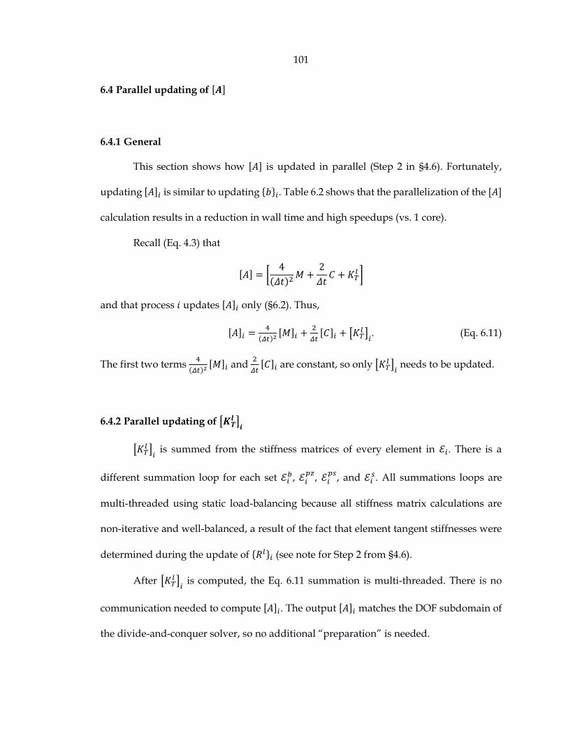
101
6.4 Parallel updating of [𝑨]
6.4.1 General
This section shows how [𝐴] is updated in parallel (Step 2 in §4.6). Fortunately,
updating [𝐴]𝑖 is similar to updating {𝑏}𝑖. Table 6.2 shows that the parallelization of the [𝐴]
calculation results in a reduction in wall time and high speedups (vs. 1 core).
Recall (Eq. 4.3) that
[𝐴] = [4
(𝛥𝑡)2𝑀 +
2
𝛥𝑡𝐶 + 𝐾𝑇
𝑙 ]
and that process 𝑖 updates [𝐴]𝑖 only (§6.2). Thus,
[𝐴]𝑖 =4
(𝛥𝑡)2[𝑀]𝑖 +
2
𝛥𝑡[𝐶]𝑖 + [𝐾𝑇
𝑙 ]𝑖. (Eq. 6.11)
The first two terms 4
(𝛥𝑡)2[𝑀]𝑖 and
2
𝛥𝑡[𝐶]𝑖 are constant, so only [𝐾𝑇
𝑙 ]𝑖 needs to be updated.
6.4.2 Parallel updating of [𝑲𝑻𝒍 ]𝒊
[𝐾𝑇𝑙 ]𝑖 is summed from the stiffness matrices of every element in ℰ𝑖. There is a
different summation loop for each set ℰ𝑖𝑏, ℰ𝑖
𝑝𝑧, ℰ𝑖
𝑝𝑠, and ℰ𝑖
𝑠. All summations loops are
multi-threaded using static load-balancing because all stiffness matrix calculations are
non-iterative and well-balanced, a result of the fact that element tangent stiffnesses were
determined during the update of {𝑅𝑙}𝑖 (see note for Step 2 from §4.6).
After [𝐾𝑇𝑙 ]𝑖 is computed, the Eq. 6.11 summation is multi-threaded. There is no
communication needed to compute [𝐴]𝑖. The output [𝐴]𝑖 matches the DOF subdomain of
the divide-and-conquer solver, so no additional “preparation” is needed.

102
Table 6.2: Wall time and speedup of parallel [A] calculation, from 60-story dynamic time-history
collapse simulation.
Number of
cores used
Wall time
(𝒉𝒓𝒔)
Speedup vs.
1-core
1
2
4
8
16
32
64
128
11.5
7.98
5.02
3.49
1.76
0.89
0.45
0.25
1.00
1.44
2.29
3.28
6.63
12.9
25.6
46.6
6.5 Parallel geometric updating
This section shows how geometric updating is performed in parallel. Table 6.3
shows that parallelization reduces geometric updating wall time. Recall (§4.6) that the
input to the geometric updating step is the newly solved {𝛥𝑈} (i.e., {𝑥} from Eq. 4.4) from
Step 3.
Geometric updating has 4 parts:
(1) Update geometric parameters of elements
(2) Update coordinates/rotations of nodes
(3) Update {𝑈𝑙}
(4) Avoid artificial unloading (adjust {𝛥𝑈}).

103
Process 𝑖 needs only to update its subdomain ℰ𝑖, 𝒩𝑖, {𝑈𝑙}𝑖, and {𝛥𝑈}𝑖. For parts (1) and (2),
multi-threaded loops across ℰ𝑖 and 𝒩𝑖 are used with static load-balancing. For parts (3)
and (4), {𝑈𝑙}𝑖 = {𝑈𝑙−1}𝑖 + {𝛥𝑈}𝑖 and {𝛥𝑈}𝑖 = {𝑈𝑙}𝑖 − {𝑈𝑙−1}𝑖 may be multi-threaded if 𝑛𝑏 is
large enough; but even if it is not multi-threaded, the operation is already parallel in the
distributed-memory sense.
Before geometric updating can occur in parallel, a communication step is needed.
Recall (§6.2) that process 𝑖 has {𝛥𝑈}𝑖. Also recall (§6.2) that some elements in ℰ𝑖 attach to
DOFs outside of process 𝑖’s DOF subdomain. Because 𝒩𝑖 depends on ℰ𝑖 (§6.2), some nodes
in 𝒩𝑖 are outside of process 𝑖’s DOF subdomain, too. Thus, to update some elements in ℰ𝑖
and some nodes in 𝒩𝑖, process 𝑖 needs some values from {𝛥𝑈} that are outside of {𝛥𝑈}𝑖—
specifically, from the 𝑚 closest DOFs from {𝛥𝑈}𝑖−1 and {𝛥𝑈}𝑖+1. An efficient
communication subroutine is created here (pseudocode in §B.3), similar to the two-step
communication used in the hybrid-parallel matrix-vector operation:
process 0{𝛥𝑈}0
𝑙𝑎𝑠𝑡
→ …{𝛥𝑈}𝑖−1
𝑙𝑎𝑠𝑡
→ process 𝑖{𝛥𝑈}𝑖
𝑙𝑎𝑠𝑡
→ …{𝛥𝑈}𝑝−2
𝑙𝑎𝑠𝑡
→ process (𝑝 − 1)
process 0{𝛥𝑈}1
𝑓𝑖𝑟𝑠𝑡
← …{𝛥𝑈}𝑖
𝑓𝑖𝑟𝑠𝑡
← process 𝑖{𝛥𝑈}𝑖+1
𝑓𝑖𝑟𝑠𝑡
← …{𝛥𝑈}𝑝−1
𝑓𝑖𝑟𝑠𝑡
← process (𝑝 − 1).
The superscripts indicate that only the last or first 𝑚 terms of {𝛥𝑈}𝑖 are passed.
The cost of the communication algorithm depends on 𝑚 and is independent from
𝑛. It is also independent from 𝑝 because each step can be done in parallel, and processes
communicate with their “nearest neighbors” only. Relative to the rest of the geometric
updating procedure (𝑚 ≪ 𝑛𝑖), the communication costs are small enough to result in
noticeable speedups relative to 1-core wall times, as observed in Table 6.3.

104
Table 6.3: Wall time and speedup of geometric updating, from 60-story dynamic time-history
collapse simulation.
Number of
cores used
Wall time
(𝒉𝒓𝒔)
Speedup vs.
1-core
1
2
4
8
16
32
64
128
0.28
0.16
0.08
0.05
0.21
0.11
0.06
0.03
1.00
1.76
3.39
6.09
1.34
2.63
4.51
8.28
6.6 Parallel convergence check
This section shows that the convergence check (Step 1 in §4.6) is automatically
performed in parallel due to the parallelization of Steps 2 – 5.
Convergence occurs if every DOF in {𝑏} converges. Because {𝑏} is split up, process
𝑖 checks {𝑏}𝑖 only. Process 𝑖 then reports a convergence status (whether subdomain 𝑖
converged) to the community of processes. If at least one process reports non-
convergence, then another global iteration is needed. Every process makes the same
global decision. In other words, global convergence occurs only if every DOF in every {𝑏}𝑖
converges.
The program has another check. Recall (§3.1) that if the maximum force residual
‖{𝑏}‖∞ grew in iteration 𝑙 − 1, then an elastic [𝐾𝑇𝑙 ] is used for iteration 𝑙. Like the

105
convergence check, this check is already parallel. Process 𝑖 determines and reports ‖{𝑏}𝑖‖∞
to the community of processes. Every process determines the same global maximum force
residual ‖{𝑏}‖∞ = 𝑚𝑎𝑥𝑖∈[0,𝑝−1]
‖{𝑏}𝑖‖∞.
Both checks use a very small collective communication step, where each process
shares a scalar with the community of processes.
6.7 Parallel input-output
This section shows how input-output is handled in parallel.
The user-input files for PFRAME3D are identical to FRAME3D. Each process
determines internally whether data is relevant for it. No additional parameter files are
needed; the user simply runs the program as shown in Table 6.4, specifying the number
of processes.
Other parallel programs, such as OpenSeesSP, make input “go through” a head-
node. The head-node reads input files then distributes the data to each process before
analysis begins—which may be a bottleneck. A head-node is not used in PFRAME3D.
Rather, each process independently reads the input files, skips irrelevant data, and keeps
relevant data, which reduces startup communication costs and the above-mentioned
bottleneck.
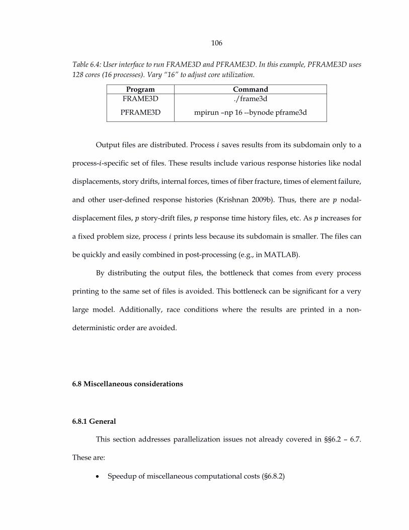
106
Table 6.4: User interface to run FRAME3D and PFRAME3D. In this example, PFRAME3D uses
128 cores (16 processes). Vary “16” to adjust core utilization.
Program Command
FRAME3D
PFRAME3D
./frame3d
mpirun –np 16 --bynode pframe3d
Output files are distributed. Process 𝑖 saves results from its subdomain only to a
process-𝑖-specific set of files. These results include various response histories like nodal
displacements, story drifts, internal forces, times of fiber fracture, times of element failure,
and other user-defined response histories (Krishnan 2009b). Thus, there are 𝑝 nodal-
displacement files, 𝑝 story-drift files, 𝑝 response time history files, etc. As 𝑝 increases for
a fixed problem size, process 𝑖 prints less because its subdomain is smaller. The files can
be quickly and easily combined in post-processing (e.g., in MATLAB).
By distributing the output files, the bottleneck that comes from every process
printing to the same set of files is avoided. This bottleneck can be significant for a very
large model. Additionally, race conditions where the results are printed in a non-
deterministic order are avoided.
6.8 Miscellaneous considerations
6.8.1 General
This section addresses parallelization issues not already covered in §§6.2 – 6.7.
These are:
Speedup of miscellaneous computational costs (§6.8.2)

107
Load-balancing in the distributed-memory layer (§6.8.3)
Conditional multi-threading (§6.8.4)
Race condition (§6.8.5)
Probabilistic fracture assignments (§6.8.6)
Shared-memory-only version of PFRAME3D (§6.8.7).
6.8.2 Speedup of miscellaneous computational costs
Table 6.5 shows that parallelization can speed up the miscellaneous computational
costs relative to 1-core wall times (i.e., everything except for §4.6’s Steps 2 – 5). These costs
include the convergence check (§6.6) and input-output (§6.7). While these speedups are
modest, they reflect a small portion of the total wall time.
Table 6.5: Wall time and speedup of miscellaneous computational costs, from 60-story dynamic
time-history collapse simulation.
Number of
cores used
Wall time
(𝒉𝒓𝒔)
Speedup vs.
1-core
1
2
4
8
16
32
64
128
1.54
1.53
1.50
1.50
0.89
0.62
0.45
0.40
1.00
1.01
1.02
1.02
1.72
2.50
3.39
3.88

108
6.8.3 Load-balancing in the distributed-memory layer
Load-balancing is an important consideration in the computation of {𝑅𝑙}𝑖, due to
the possibly imbalanced local iterations of multi-segmented elements. The shared-
memory layer accounts for this imbalance with the sorted dynamic load-balancing scheme
(§6.3.2). A similar type of imbalance can be observed in the distributed-memory layer. If
one process is slower than others (e.g., because some parts of the building yield more than
others), the other processes must wait. But if dynamic load-balancing is implemented for
the distributed-memory layer, large amounts of element and node data must be
communicated (e.g., the fiber histories of every fiber from every fiber segment in each
element), which may increase the {𝑏} calculation’s overall wall time. It is a concern for
future study.
6.8.4 Conditional multi-threading
There are minor loops that are not multi-threaded because overhead likely costs
more than the loop itself. It is possible to study the tipping-point size (where
parallelization outweighs multi-threading overhead cost) and implement conditional
threads—parallel only if past the tipping point. This study is not done here, and results
are expected to be processor-specific.
6.8.5 Race condition
Parallel programs with a shared-memory layer may suffer from the so-called race
condition, where core 𝑗 may edit a variable that core 𝑘 is using. This type of bug is not
deterministic and difficult to track because it depends on the relative computational

109
speeds of cores 𝑗 and 𝑘. Although not detailed here, considerable effort is taken to avoid
race conditions. §7 indicates that race-condition problems are absent from PFRAME3D.
6.8.6 Probabilistic fracture assignments
Recall that FRAME3D simulates probabilistic beam fractures (§2.4). At the start of
the program, a random number generator is used. A user may want a reproducible
“random” sequence of numbers, and hence specify a seed. Thus, for a given seed, the fiber
fracture assignments in PFRAME3D match FRAME3D. The random number generator in
PFRAME3D produces identical results to that of FRAME3D, regardless of process or core
count.
6.8.7 Shared-memory-only version of PFRAME3D
A shared-memory-only version of PFRAME3D is also created using the special
case of 𝑝 = 1. Here, the multi-threaded blocked solver (§5.3) is used for Step 3 (instead of
the divide-and-conquer solver). Thus, 𝑖 = 0, [𝐴] = [𝐴]0, {𝑥} = {𝑥}0, ℰ = ℰ0, 𝒩 = 𝒩0, etc.
This version is suitable for solving small problems in parallel.
6.9 Conclusion
In this chapter, the entirety of FRAME3D has been made parallel. Reductions in
wall time are observed for every step outside of the direct solver (Steps 1, 2, 4, and 5).

110
Recall (§5.6) that for the 60-story building dynamic time-history collapse
simulation, Steps 1, 2, 4, and 5 take 69.4 hrs to complete with 1 core. Due to 128-core
parallelization, the 69.4 hrs is reduced to 1.95 hrs. Also recall (§5.6) that, for the same
simulation, the 128-core divide-and-conquer solver uses 3.74 hrs. Thus, combining §5 and
§6, the overall 128-core simulation wall time is (1.95 + 3.74) hrs = 5.69 hrs.
The remainder of Part II (i.e., §7) demonstrates PFRAME3D’s ability to produce
the same results as FRAME3D, and further showcases PFRAME3D’s computational
performance, using three example structures of varied sizes.

111
Chapter 7
Overall Parallelization Results
7.1 General
PFRAME3D is described in §4 – 6. In the present chapter, two types of comparisons
are made between PFRAME3D and an optimized 1-core version of FRAME3D (that also
includes the revisions made in Part I). The first comparison demonstrates that PFRAME3D
produces time-history structural responses that are nearly identical to that of FRAME3D
and that any discrepancies are negligible. The second comparison demonstrates that
PFRAME3D uses less overall wall time due to parallelization. Three example structures
are used:

112
the water-tank tower from Bjornsson and Krishnan (2014) (§7.2)
an 18-story building from Mourhatch (2015) (§7.3)
the 60-story tube building from §8 (§7.4).
All three structures are subjected to collapse-causing dynamic time-history ground
motions. In all cases, displacement response histories are saved and simulations are timed
with various degrees of parallelism (i.e., core usage). The performance results from the
three simulations are compared in §7.5.
7.2 Results using a small structure
This section shows that the output of the shared-memory-only PFRAME3D is
nearly identical to that of FRAME3D and that wall time reductions due to parallelization
are significant even for a small structure.
The water-tank tower from Bjornsson and Krishnan (2014) is a braced-frame
structure with:
𝑛 = 252
𝑚 = 102
144 EF5 elements
18 PS elements
12 spring elements
44 nodes.

113
Details regarding the water-tank tower’s elevation, plan, and member sizes can be found
in Bjornsson and Krishnan (2014). It was not designed according to any particular building
code. The water-tank tower is subjected to the Kobe earthquake ground motion at
Takatori (Figure E.1), scaled at 37.3%—the same 3-component ground motion in §3.7. The
simulation is terminated at 𝑡 = 38 𝑠𝑒𝑐 (7600 dynamic time steps are used), when the
water-tank tower is clearly collapsing. The collapse configuration at termination is shown
in Figure 7.1 for visualization.
Because the number of processes 𝑝 allowed by the divide-and-conquer solver
(§5.4) is limited according to Eq. 5.22, or 𝑝 ≤𝑛
2(𝑚−1)=
252
2(102−1)≈ 1.24, only 1 process may
be used; thus, the shared-memory-only version of PFRAME3D (§6.8.7) is used with up to
8 cores (1 process).
This example indicates that the shared-memory layer of PFRAME3D produces
consistent results; Figure 7.2 shows that the roof displacement histories agree regardless
of core usage. Against the 1-core “X Displacement” history shown in Figure 7.2, the root-
mean-squared error of the 8-core “X Displacement” history is 6.55 × 10⁻⁵ 𝑚, which can
be considered as negligible for the present context.
In terms of performance, Table 7.1 shows that the 1-core 3.58 hr simulation is
reduced with 8 cores to 1.23 hrs.

114
Figure 7.1: Isometric views of water-tank tower at t=0 sec (left) and t=38 sec (right) using 37.3%
Kobe earthquake ground motion at Takatori (Figure E.1). Elements that failed during analysis are
not shown. Deformations are unamplified.
Table 7.1: Overall parallelization speedup for water-tank tower collapse simulation.
Number of
cores used
Wall time
(ℎ𝑟𝑠)
Speedup vs.
1-core
1
2
4
8
3.58
2.27
1.55
1.23
1.00
1.58
2.31
2.89

115
Figure 7.2: Roof displacement histories of water-tank tower (from the node initially at X=4.064 m,
Y= 8.128 m, Z= 48.768 m) subjected to 37.3% Kobe earthquake ground motion at Takatori (Figure
E.1). The results from 1-, 2-, 4-, and 8-core analysis are nearly identical.

116
7.3 Results using an 18-story building
This section shows that the output of PFRAME3D (the complete hybrid-parallel
version) matches that of FRAME3D and that wall time is reduced more for a medium-
sized tall building structure. The 18-story building (often referred to as the Canoga Park
building), designed according to the UBC 94 with S2 soil conditions, from Mourhatch
(2015), is a braced-frame building with:
𝑛 = 3966
𝑚 = 289
258 PH elements
282 EF3 elements
492 EF5 elements
216 PZ elements
517 PS elements
30 spring elements
760 nodes.
Details regarding the 18-story building’s elevation, plan, and member sizes can be found
in Mourhatch (2015). This building is subjected to a five-cycle idealized acceleration
square wave with peak ground velocity 𝑃𝐺𝑉 = 1.375𝑚 𝑠⁄ and period 𝑇 = 5.75 𝑠𝑒𝑐 (Figure
E.2). The simulation is set to terminate when the peak displacement history exceeds 300 𝑖𝑛
(~7 𝑚), when the building is clearly collapsing. The collapse configuration at termination
is shown in Figure 7.3 for visualization. Because 𝑛
2(𝑚−1)=
3966
2(289−1)≈ 6.88 (Eq. 5.22), up to
48 cores (6 processes) are used.

117
Figure 7.4 shows that the roof displacement histories agree regardless of core
usage. 76 displacement histories (from throughout the building) are used to compare the
1-core and 48-core results, and the maximum observed root-mean-square error is 3.77 ×
10−11 𝑚, which can be considered as negligible for the present context.
Figure 7.5 (top) shows that the parallelization of the {𝑏} & [𝐴] update calculations
contributes the most to the “Total” wall time reduction from 30.5 hrs with 1 core, to 2.95
hrs with 48 cores. The shift to distributed-memory computing begins with 16 cores, so a
penalty can be seen then (i.e., from 8 cores to 16 cores in Figure 7.5). For example, the
parallel geometric updating, in which communication is significant, slows down at 16
cores but speeds up as 48 cores is approached. Additionally, the divide-and-conquer
factorization is slower than the 8-core blocked factorization, as a result of “fill-in” and the
fact that 𝑝 is nearing the Eq. 5.22 limit (recall §5.4). Nevertheless, because the parallel
speedup of the {𝑏} & [𝐴] update calculations is more significant than the parallel
slowdown of the divide-and-conquer solver and parallel geometric updating, the lowest
wall time of 2.95 hrs is achieved with 48 cores, a speedup of 10.3.

118
Figure 7.3: Isometric views of 18-story building at t=0 sec (left) and t=22.7 sec (right) subjected to
the acceleration square wave ground motion (Figure E.2). Elements that failed during analysis are
not shown. Deformations are unamplified.

119
Figure 7.4: Displacement histories at penthouse roof of 18-story building subjected to an idealized
five-cycle acceleration square wave with peak ground velocity PGV=1.375 m⁄s and period T=5.75
sec (Figure E.2). The results from 1-, 8-, 32-, and 48-core analysis are nearly identical.

120
Figure 7.5: Performance summary for 18-story collapse simulation. Wall time of total and various
steps (top), and speedup vs. optimized 1-core code (bottom).
0.001
0.01
0.1
1
10
100
1 2 4 8 16 32 64
Wal
l tim
e (h
r)
Number of cores used (N)
Total A=LL^T LL^Tx=b {b} & [A] Update geo. Misc.
0
2
4
6
8
10
12
14
1 2 4 8 16 32 64
Spee
du
p (
T(1
,1)/
T(N
,1))
Number of cores used (N)

121
7.4 Results using a 60-story building simulation
This section further shows that the output of PFRAME3D (the complete hybrid-
parallel version) agrees with that of FRAME3D and that wall time is reduced even more
for very tall building structures. The large structure considered here is the 60-story
moment-frame tube building designed according to the UBC 94 from §8 of the current
report, with:
𝑛 = 30,606
𝑚 = 514
1496 PH elements
3840 EF3 elements
4348 EF5 elements
4080 PZ elements
4320 PS elements
77 spring elements
4421 nodes.
The EF3 and EF5 elements have probabilistic fiber fracture assignments (§§8.3.2 – 8.3.3,
brittle case with 𝑠𝑒𝑒𝑑 = 1). Details regarding the 60-story building’s elevation, plan, and
member sizes can be found in §8.2. The building is subjected to the Denali earthquake at
Pump station #10 (Figure E.3). This ground motion is chosen because the building
approaches collapse slowly (~40 𝑠𝑒𝑐 in earthquake time), providing greater opportunity
to check whether unforeseen race conditions are present. The simulation is set to terminate
when the peak displacement history exceeds 300 𝑖𝑛 (~7 𝑚), when the building is clearly

122
collapsing. The collapse configuration at termination is shown in Figure 7.6 for
visualization. Because 𝑛
2(𝑚−1)=
30606
2(514−1)≈ 29.8 (Eq. 5.22), up to 232 cores (29 processes) are
used.
Figure 7.7 shows that the roof displacement histories agree regardless of core
usage. 122 displacement histories (X and Y displacements from the centroids of the 61
floors) are used to compare the 1-core and 128-core results, and the maximum observed
root-mean-square error is 2.78 × 10⁻⁶ 𝑚, which can be considered as negligible for the
present context. It is worth noting that every element type (§2) is included in this model,
and that probabilistic fiber fracture assignments are included in the EF3 and EF5 elements.
Figure 7.7 (top) shows that parallelization reduces the “Total” wall time from 83.6
hrs (1-core) to 5.69 hrs (128-cores). At 1 core, the {𝑏} & [𝐴] update calculations are the most
expensive, but once extended to distributed-memory computing (≥16 cores), the divide-
and-conquer factorization becomes the most expensive step.
Unfortunately, the divide-and-conquer factorization does not exhibit speedups as
impressive as that of the parallel {𝑏} & [𝐴] update calculations. Nevertheless, the
parallelization of {𝑏} & [𝐴] calculations is significant enough that the “Total” speedup
reaches 14.7 with 128 cores. Additionally, as shown in Figure 7.9 (plot of the wall time of
each step as a function of earthquake time, from the 128-core simulation of the 60-story
building collapse), the {𝑏} & [𝐴] update calculations become more significant as the
building yields and elements are more nonlinear, especially at the last time steps of the
simulation (as collapse is approached).
The slight “parallel slowdown” of the “Total” computation at 232 cores (“Total”
wall time is 5.69 hrs with 128 cores and 5.74 hrs with 232 cores) is attributed to the divide-

123
and-conquer, which as mentioned in §5.4, is less efficient as 𝑝 nears the Eq. 5.22 limit for
a fixed problem size. Still, it should be noted that for an even taller building, the Eq. 5.22
limit is increased (assuming that 𝑛 increases much faster than 𝑚), such that higher core
counts may be used effectively. Additionally, the other steps in Figure 7.8 are shown to
be faster with 232 cores. It is of interest in a future study to either improve the divide-and-
conquer solver (e.g., by accounting for sparsity within the narrow band) or altogether
remove the direct solver (e.g., by solving the global equation of motion using a nonlinear
conjugate gradient approach). The present hybrid-parallel framework is expected to be
able to accommodate such changes.

124
Figure 7.6: Isometric views of 60-story building at t=0 sec and t=41.9 sec subjected to the Denali
earthquake ground motion at Pump station #10 (Figure E.3). Elements that failed during analysis
are not shown. Deformations are unamplified.

125
Figure 7.7: Displacement histories at the roof centroid of the 60-story building subjected to the Denali earthquake ground motion at Pump station #10 (Figure E.3). The results from 1-, 8-, 128-, and 232-core analysis are nearly identical.
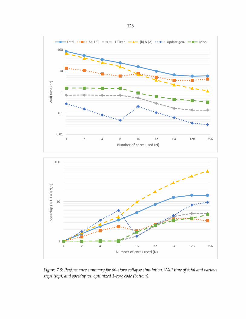
126
Figure 7.8: Performance summary for 60-story collapse simulation. Wall time of total and various
steps (top), and speedup vs. optimized 1-core code (bottom).
0.01
0.1
1
10
100
1 2 4 8 16 32 64 128 256
Wal
l tim
e (h
r)
Number of cores used (N)
Total A=LL^T LL^Tx=b {b} & [A] Update geo. Misc.
1
10
100
1 2 4 8 16 32 64 128 256
Spee
du
p (
T(1
,1)/
T(N
,1))
Number of cores used (N)

127
Figure 7.9: Wall time (sec) per earthquake-simulation time step, from 60-story building subjected
to the Denali earthquake ground motion at Pump station #10 (Figure E.3). PFRAME3D with 128
cores is used. The “spikes” in the {b} & [A] update wall times are a result of load imbalances in the
distributed-memory layer (§6.8.3).
7.5 Maximum speedups
A more holistic understanding of PFRAME3D’s performance can be obtained by
comparing the “Total” performance results of the three buildings with each other, as is
done in Figure 7.10. For the water-tank tower collapse simulation, PFRAME3D achieves a
maximum speedup of 2.89 with 8 cores; for the 18-story building collapse simulation, it
achieves a maximum speedup of 10.3 with 48 cores; and for the 60-story building collapse
simulation, it achieves a maximum speedup of 14.7 with 128 cores.

128
An additional curve is constructed on Figure 7.10 (bottom) by connecting the
maximum speedups attained for the three structures. An upward trend can be seen, which
suggests that as building height increases, additional cores may be used to achieve a
higher speedup.
The above comparison is similar to a weak-scaling study. However, it cannot be
appropriately classified as such because the per-core workloads vary between the three
cases. For example, because each structure has a different bandwidth, the divide-and-
conquer per-core workload varies. Or, the number of elements per floor is varied; e.g., the
60-story building has more frame elements per floor than the 18-story building. It is also
important to note that the three simulations themselves are very different. Three different
ground motions are used, the collapse mechanisms form at different times, and the water-
tank tower and 18-story building are braced-frame buildings while the 60-story building
is a moment-frame tube building.
Nevertheless, Figure 7.10 indicates that parallel speedup increases with building
height. It is not unreasonable to suggest that even higher speedups than shown in Figure
7.10 are possible if PFRAME3D is applied to even taller buildings (e.g., a 100-story
building).
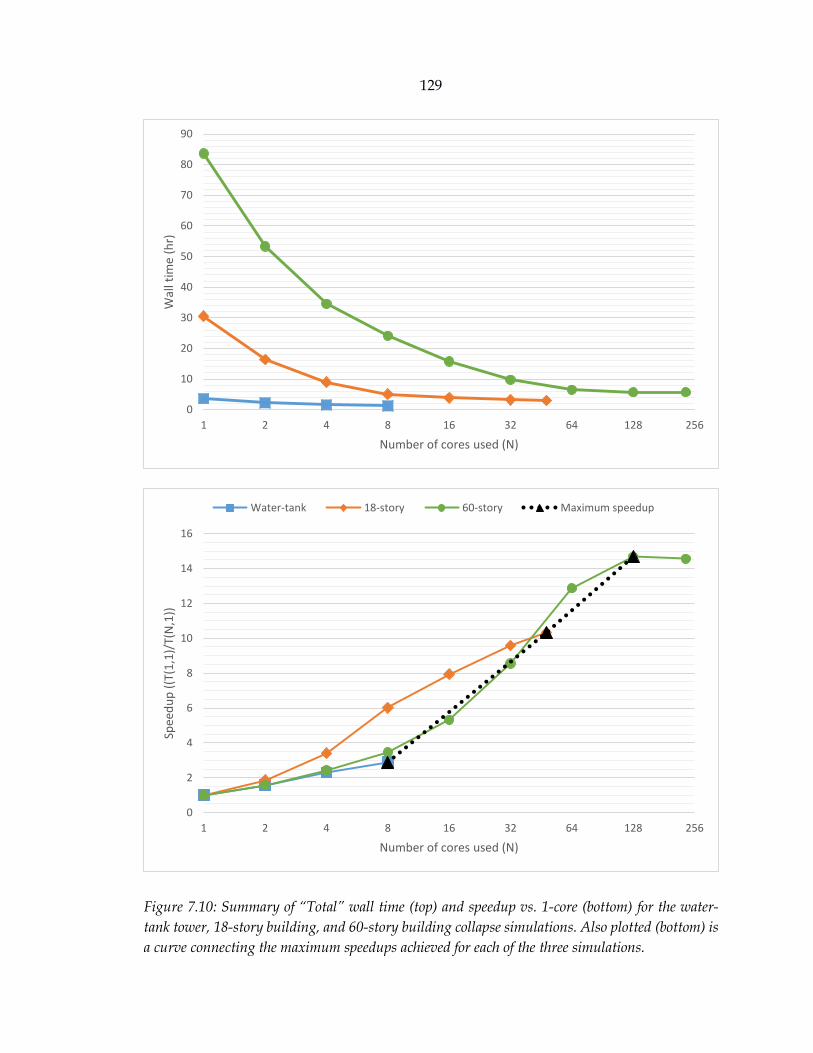
129
Figure 7.10: Summary of “Total” wall time (top) and speedup vs. 1-core (bottom) for the water-
tank tower, 18-story building, and 60-story building collapse simulations. Also plotted (bottom) is
a curve connecting the maximum speedups achieved for each of the three simulations.
0
10
20
30
40
50
60
70
80
90
1 2 4 8 16 32 64 128 256
Wal
l tim
e (h
r)
Number of cores used (N)
0
2
4
6
8
10
12
14
16
1 2 4 8 16 32 64 128 256
Spee
du
p (
(T(1
,1)/
T(N
,1))
Number of cores used (N)
Water-tank 18-story 60-story Maximum speedup

130
7.6 Conclusion
Therefore, using the three example dynamic time-history collapse simulations in
§§7.2 – 7.4, PFRAME3D is shown to produce output that is nearly identical to that of
FRAME3D. Race condition problems are not observed in any of the three cases.
Still, it should be noted that round-off errors due to floating-point arithmetic can
cause parallel computations to produce slightly different results than that of the 1-core
computations (Goldberg 1991, Villa et al. 2009). For example, the mathematical property
of associativity does not necessarily hold in optimized parallel libraries like Intel MKL.
Or, elements may update the global {𝑅𝑙} (§6.3.2) and [𝐾𝑇𝑙 ] (§6.4.2) in a different order than
the 1-core case, leading to a slightly different {𝑅𝑙} and [𝐾𝑇𝑙 ] (again, due to non-
associativity). It is possible to use fully deterministic versions of the Intel MKL routines,
or use static load-balancing such that {𝑅𝑙} and [𝐾𝑇𝑙 ] are assembled by the same sequence
of elements as the 1-core case. However, these fixes are not optimal in terms of parallel
performance, and so are not implemented here. Additionally, displacement-history root-
mean-square errors are observed to be ~10−5 𝑚 or less, and Figure 7.2, Figure 7.4, and
Figure 7.7 show that the resulting collapse mechanisms are reproducible regardless of
parallelization. Therefore, it can be stated that these discrepancies are negligible in the
overall context of building analysis.
Maximum speedups are shown to grow with the height of the building, and a 60-
story dynamic time-history collapse simulation is completed in 5.69 hours with 128 cores.
Thus, it can be said that PFRAME3D is suited for the efficient computation of tall building
response due to ground motion.

131
PART III
Application and Conclusions
132
Chapter 8
Application to a 60-story steel building
8.1 General
In this chapter a 60-story example building is developed and analyzed, in order to
showcase PFRAME3D’s capability to perform collapse analysis on very tall buildings. The
design satisfies UBC 94 load and stiffness criteria, and has a typical mass distribution for
office buildings. It has a 6.16-second fundamental period, which is typical for buildings of
its height. However, the building shows atypical moment-frame behavior because of the
use of very closely spaced columns (8 𝑓𝑡 or 2.4384 𝑚 center-to-center) and very deep
beams (up to 30 𝑖𝑛 or 0.762 𝑚). Beams in this configuration are likely to yield in shear, but

133
neither the EF3 (§2.4) or EF5 (§2.5) element can capture nonlinear shear. A more realistic
building model, with shallower beams and columns less closely spaced, will be designed
in a future project. Nevertheless, this test case is sufficient for the current report and
PFRAME3D is shown to be useful for studying very tall buildings subjected to strong
ground motions. Observations such as multi-story quasi-shear band collapse mechanisms
(similar to Krishnan and Muto 2012) are noted. This chapter is organized as follows:
Building design and description (§8.2)
Modeling considerations (§8.3)
Building analyses and results (§8.4).
8.2 Building description and design
8.2.1 Building description
The building considered in this chapter is a moment-frame (MF) tube structure.
The general behavior of tube structures is well explained in Smith and Coull (1991) and
briefly recounted in §C for convenience.
The 60-story example building is designed with typical and 1st-story plans shown
in Figure 8.1 and Figure 8.2, respectively. Story height is 12.5 𝑓𝑡 (3.81 𝑚) at levels 2 – 60,
and 15 𝑓𝑡 (4.572 𝑚) at level 1. The plan is a square to take advantage of symmetry. Beam
and column sizes are chosen every 4 stories as shown in Table 8.1. The properties of non-
standard sections can be found in §D. For simplicity, all MF beams are identical within a
floor level, all interior MF columns are identical within a story level, all gravity columns

134
are identical within a story level, etc. Column splices are located at every odd story level
above first story. Design considerations are discussed in §8.2.2. Modal characteristics and
mode shapes of the building are shown in Table 8.2 and Figure 8.3, respectively.
Figure 8.1: Typical plan (3rd floor to Roof) of 60-story example tube building, featuring closely-
spaced columns.

135
Figure 8.2: Plan for 2nd floor of 60-story example tube building, featuring transfer girder.

136
Table 8.1: Summary of column and beam sizes for 60-story example building.
Story
levels
Moment frame Gravity frame
Floor
levels
Moment
frame
Corner
columns
Interior
columns
Columns Beams
57 – 60
53 – 56
49 – 52
45 – 48
41 – 44
37 – 40
33 – 36
29 – 32
25 – 28
21 – 24
17 – 20
13 – 16
9 – 12
5 – 8
2 – 4
1
W14X82
W14X159
W14X176
W14X211
W14X233
W14X283
W14X342
W14X370
W14X398
W14X426
W14X455
W14X500
W14X550
W14X665
W14X873
28”X28” box*
W18X71
W18X97
W18X119
W21X147
W24X176
W27X194
W30X211
W30X261
W33X291
W33X318
W33X354
W36X395
W36X441
W36X529
W36X723
W36X925**
W12X136
W14X193
W14X257
W14X342
W14X426
W14X500
W14X550
W14X605
W14X665
W14X730
W14X808
W14X873
24”X24” box*
24”X24” box*
26”X26” box*
26”X26” box*
58 – Roof
54 – 57
50 – 53
46 – 49
42 – 45
38 – 41
34 – 37
30 – 33
26 – 29
22 – 25
18 – 21
14 – 17
10 – 13
6 – 9
3 – 5
2
W18X46
W18X60
W21X62
W21X62
W21X62
W21X68
W21X73
W21X73
W21X83
W21X93
W24X103
W24X103
W27X114
W27X114
W30X148
W40X324***
* Non-standard section, see §D.
** For column lines that extend to the ground.
*** Transfer girder.
Table 8.2: Modal periods of 60-story example building.
Mode Type Period (s)
1, 2
3
4, 5
6
7, 8
1st translational
1st torsional
2nd translational
2nd torsional
3rd translational
6.16
3.18
2.12
1.32
1.26

137
Figure 8.3: Elevation view of the 60-story example building’s first three translational modes along
a single direction.
8.2.2 Building design
The 60-story building is assumed to be located in downtown Los Angeles (DTLA).
Because some high-rise DTLA buildings were designed according to pre-Northridge
building code, design loads are determined according to the 1994 Uniform Building Code
(UBC 94). The building’s beams and columns are proportioned using the Allowable Stress
Design (ASD) procedure found in the Specification for Structural Steel Buildings: Allowable
Stress Design and Plastic Design (AISC 335-89). Design software ETABS is used throughout
the entire design procedure.

138
The basic ASD load combinations (UBC 94 §1603.6) considered are:
𝐷 + 𝐿
𝐷 + 𝐿 ±𝑊
𝐷 + 𝐿 ± 𝐸
where 𝐷, 𝐿, 𝑊, and 𝐸 are dead, live, wind, and earthquake loads, respectively. Columns
also satisfy (UBC 94 §2211.5.1):
1.0𝐷 + 0.7𝐿 ± 3 (𝑅𝑤
8)𝐸
0.85𝐷 ± 3(𝑅𝑤
8)𝐸
where 𝑅𝑤 accounts for material overstrength.
Design dead loads are according to Table 8.3. Combined, the typical floor dead
load (without beam/column self-weight and cladding) is 76 𝑝𝑠𝑓 (3.64𝑘𝑁
𝑚2) and the roof
dead load (without beam and column self-weight) is 64 𝑝𝑠𝑓 (3.06𝑘𝑁
𝑚2). Cladding is
applied around the building perimeter.
Table 8.3: Design dead loads.
Dead load 𝒑𝒔𝒇 (
𝒌𝑵
𝒎𝟐)
MF beams and columns
Gravity columns
(Primary) gravity beams
(Secondary) gravity beams
Concrete slab
Carpet/finish
Mechanical, ceiling, etc.
Partitions
Cladding
Self-weight
Self-weight
Self-weight
6 (0.29)
50 (2.39)
2 (0.096)
8 (0.38)
10 (0.48)
15 (0.72)

139
The building is intended to be an office building, and the design floor live loads
are 50 𝑝𝑠𝑓 (2.39𝑘𝑁
𝑚2) uniformly distributed (UBC 94, Table 16-A), except at the roof where
live loads are 20 𝑝𝑠𝑓 (0.96𝑘𝑁
𝑚2) uniformly distributed (UBC 94, Table 16-C).
Design wind loads are applied as static forces according to the national standard
ASCE 7-93 §6 (UBC 94 §1613). The wind-design parameters used are summarized in Table
8.4 as defined in the ASCE 7-93 §6. Story-drift ratios are checked to be within 1
400 using the
10-year wind and a 1st order analysis (Griffis 1993).
Seismic consideration is important in DTLA. A static lateral-force procedure (UBC
94 §1628.2) is an approximation of earthquake loads; while it is convenient for short
buildings, earthquakes are dynamic and often bring out the higher-mode effects in tall
buildings. Thus, the code requires a dynamic lateral-force procedure for buildings taller
than 240 𝑓𝑡 (73.152 𝑚) (UBC 94 §1627.8.3). Beams and columns are proportioned
according to the Response Spectrum Method (UBC 94 §1629.5) scaled to 90% of the static
procedure base shear. Overall building stability (P-Δ), individual column stability (P-δ),
and accidental torsion are considered. The seismic design parameters used are
summarized in Table 8.5 as defined in the UBC 94. Story drifts due to seismic loads are
checked to remain below a maximum allowable limit of 𝛥𝑎 = 0.0025ℎ𝑠𝑥 using 𝐶𝑠 = 0.012
(UBC 94 §1628.8).
Beams are proportioned to satisfy biaxial bending and shear strength demands.
Although it is not uncommon for designers to proportion MF beams to yield in flexure
(before shear), this check is not found to be explicitly specified in the UBC 94 as a beam
proportioning issue and is not done here. Columns are proportioned to satisfy combined

140
axial and biaxial bending stresses using the Effective Length Method (AISC 335-89 §C2.2)
and strong-column-weak-beam criteria. Beams and columns are also proportioned to
satisfy acceptable width-thickness ratios. Doubler plates are added to PZs as prescribed
by the code.
At the upper story levels, wind drifts and seismic stresses govern the beam design,
and seismic stresses govern the column design. At the lower story levels, seismic stresses
govern the column design, and beam sizes are increased so as to limit the Effective Length
Method K-factor enough to satisfy the allowable column stress criteria.
Figure 8.4 shows that the maximum wind drift ratios due to the 10-year wind load
are under 1
400= 0.0025, and the maximum seismic drift ratios are under
0.03
𝑅𝑤= 0.0025. Due
to symmetry only one loading direction is shown. The “total” drift is reported by the
design program ETABS and scaled to reflect the appropriate drift-level loads. The
“bending” drift is approximated based on the rotation of the entire story level. The “shear”
drift is the difference between “total” and “bending” drifts.
Table 8.4: ASCE 7-93 wind design parameters for the 60-story example building.
Parameter Value
𝑉
Exposure category
𝐼
�̅�
𝐶𝑝
70 𝑚𝑝ℎ (31.3 𝑚/𝑠)
B
1.00
1.20
0.8 (windward)
-0.5 (leeward)

141
Table 8.5: UBC 94 seismic design parameters for the 60-story example building.
Parameter Value
𝐶𝑠
𝑍
𝐼
𝐶
𝑆
𝑇
𝑅𝑤
0.030 (strength)
0.012 (drift)
0.40
1.00
0.36
1.00
6.54
12
Figure 8.4: Maximum wind drift ratios using ASCE 7-93 (left) and maximum seismic drift ratios
using UBC 94 Response Spectrum Method (right) for the 60-story building.
0
10
20
30
40
50
60
0 0.0005 0.001 0.0015 0.002 0.0025
Sto
ry le
vel
Maximum wind drift ratio
Total Bending Shear
0
10
20
30
40
50
60
0 0.0005 0.001 0.0015 0.002
Sto
ry le
vel
Maximum seismic drift ratio
Total Bending Shear
142
8.3 Modeling considerations
8.3.1 General
This section outlines the assumptions used to model the 60-story example building
in PFRAME3D. It is organized as follows:
Beams (§8.3.2)
Columns (§8.3.3)
Beam-column joints (§8.3.4)
Floor/roof slabs (§8.3.5)
Foundations (§8.3.6)
Soil-structure interaction (§8.3.7)
Gravity loads and mass (§8.3.8)
Damping (§8.3.9)
Miscellaneous parameters (§8.3.10).
3D models are created because 3D effects are present in tube buildings. Corner columns
belong to two orthogonal frames, and so may be subject to biaxial bending. Torsion may
be present due to probabilistic weld-fracture assignments, which can result in asymmetric
yielding from bi-directional shaking.
8.3.2 Beams
MF beams are modeled as EF3 elements (§2.4), where each fiber segment is 3% of
the total beam length (calibrated in Krishnan 2003, based on material properties). The
material model of each fiber (Figure 3.7) is defined by

143
𝐸 = 29000 𝑘𝑠𝑖 (200 𝐺𝑃𝑎)
𝜎𝑦 = 50.0 𝑘𝑠𝑖 (345 𝑀𝑃𝑎)
𝐸𝑠ℎ = 580 𝑘𝑠𝑖 (4.00 𝑀𝑃𝑎)
𝜀𝑠ℎ = 0.012
𝜎𝑢 = 65 𝑘𝑠𝑖 (448 𝑀𝑃𝑎)
𝜀𝑢 = 0.160
𝜎𝑓𝑖𝑛 = 0.60𝜎𝑢.
MF beams have rigid end connections. Perfect and brittle weld cases are considered. The
perfect case assumes full ductility in a steel fiber, i.e., the tensile fracture strain is set to the
tensile rupture strain, or 𝜀𝑓 = 𝜀𝑟 (§3.7). But using perfect welds may be unconservative,
especially for pre-Northridge buildings (Hall 1998, Krishnan and Muto 2012). That is
partly because MF assemblages used in experiments were smaller than in real buildings,
and the stress intensity factor 𝐾 (in fracture mechanics) scales unconservatively with size.
Additionally, field conditions may be non-ideal for producing perfect welds.
Thus, fracture-prone (brittle) welds are also modeled; if the tensile fracture strain
(𝜀𝑓) is exceeded, the fiber can no longer carry tensile stresses. 𝜀𝑓 is handled according to a
probabilistic 10-point distribution (10% probability for each point). The distribution used
in Krishnan and Muto (2012) is used here. For a beam’s bottom flange, 𝜀𝑓 = 0.9𝜀𝑦, 2𝜀𝑦, 5𝜀𝑦,
15𝜀𝑦, and 40𝜀𝑦 each have a 20% probability of assignment. For a beam’s web and top
flange, 𝜀𝑓 = 10𝜀𝑦 & 20𝜀𝑦 each have a 30% probability of assignment, and 𝜀𝑓 = 40𝜀𝑦 & 80𝜀𝑦
each have a 20% probability of assignment.

144
Gravity-only beams are modeled as PH elements (§2.3) with pinned end
connections. Only primary gravity beams (that attach directly to columns) are included;
no secondary beams (beams framing into beams) are modeled.
8.3.3 Columns
MF and gravity columns are modeled as EF5 elements (§2.5) to efficiently account
for geometric nonlinearity and column splices. Each fiber segment is 3% of the total
column length. Material properties match that of the beams. The center fiber segment is
used to model column splices with two weld cases: perfect and brittle. For brittle column
splices, 𝜀𝑓 = 10𝜀𝑦 & 20𝜀𝑦 each have a 30% probability of assignment, and 𝜀𝑓 = 40𝜀𝑦 &
80𝜀𝑦 each have a 20% probability of assignment.
8.3.4 Beam-column joints
The joints between beams and columns are modeled as PZ elements (§2.6). Its
linear-quadratic ellipsoidal material model (Figure 2.11) is defined by
𝐺 = 11600.0 𝑘𝑠𝑖 (80.0 𝐺𝑃𝑎)
𝜏𝑦 = 28.8675 𝑘𝑠𝑖 (199.03 𝑀𝑃𝑎).
8.3.5 Floor/roof slabs
Slabs are modeled as diaphragm elements (§2.7). Its linear-elastic material model
is defined by
𝐸 = 3605.0 𝑘𝑠𝑖 (24.86 𝐺𝑃𝑎)
𝜈 = 0.30.

145
Each slab is 6.25 𝑖𝑛 (0.159 𝑚) thick, and configured to laterally constrain every node at a
floor without adding global nodes, as shown in Figure 8.5. If the beams on both sides of a
column fail, the diaphragm prevents the column from two-story buckling.
Figure 8.5: Layout of diaphragm elements in a typical floor level.

146
8.3.6 Foundation
A mat foundation, typical in DTLA, is approximated using elastic beams (§2.3) at
ground level (Figure 8.6). The beams have stiffness properties that match a 10 𝑓𝑡 (3.3 𝑚)
deep foundation with an elastic material model where 𝐸 = 3605.0 𝑘𝑠𝑖 (24.86 𝐺𝑃𝑎). The
beams are rigidly connected. Subterranean levels are not modeled.
Figure 8.6: Foundation and soil modeling for 60-story example building.
8.3.7 Soil-structure interaction
To model soil-foundation-structure interaction, springs (§2.8) are attached at
ground level to the foundation beams (§8.3.6) as shown in Figure 8.6. Horizontal springs
are placed orthogonal to the perimeter at the base, and vertical springs are distributed

147
throughout the footprint of the base. The vertical springs automatically account for
rocking. All springs are elastic. The springs’ combined effect is tuned to yield a 10%
fundamental-period increase for Building 1 (the 6.16 𝑠𝑒𝑐 fundamental period in Table 8.2
includes soil-structure interaction), whilst maintaining a horizontal-to-vertical soil
stiffness ratio of 1-to-1.27 determined by the shallow-foundation equations from NIST
GCR 12-917-21 §2.2; these equations depend on the soil’s shear modulus 𝐺, Poisson’s ratio
𝜈, and the dimensions of the shallow foundation. The stiffness of an individual spring is
directly proportional to its “tributary” perimeter (horizontal springs) or area (vertical
springs).
8.3.8 Gravity loads and mass
Vertical gravity forces are applied at every global node (to form {𝑓𝑔} in Eq. 2.2),
before and throughout dynamic analysis. Additionally, masses that represent the inertia
of the building are applied at every global node (to form [𝑀] in Eq. 2.2). 100% dead loads
and 25% live loads are used for both gravity loading and masses. Rotational-DOF masses
are not included.
8.3.9 Damping
Rayleigh damping is used. As mentioned in §3.6, there are some unrealistic effects
associated with Rayleigh damping that are significant before and during collapse but are
not addressed here. These effects should be taken into consideration when interpreting
results (Hall 2005; ATC 72 §2.4.4.3). 2% damping is used because it is typical for a 60-story
building (ATC 72 §2.4.3.1). To capture the effects of significant higher modes, the 2%

148
damping limits are anchored as shown in Figure 8.7 at the fundamental period 𝑇1 and at
0.2𝑇1 (ATC 72 §2.4.4). Because 𝑇1 = 6.16 𝑠𝑒𝑐 and 0.2𝑇1 = 1.23 𝑠𝑒𝑐, 𝑎0 = 0.0340 and 𝑎1 =
0.00654. In other words, the first three translational and first two torsional modes are
damped at or below 2%. For future work, capped dampers will be included into the
PFRAME3D framework.
8.3.10 Miscellaneous parameters
The tolerance, convergence, and Newmark parameters used in analysis are shown
in Table 8.6. Also, analysis is automatically terminated if any node’s displacement exceeds
300 𝑖𝑛 (7.62 𝑚), when the building is clearly collapsing.
Figure 8.7: Damping ratio vs. period for 60-story example building.
0
0.01
0.02
0.03
0.04
0.05
0.06
0 1 2 3 4 5 6 7 8 9 10
Dam
pin
g ra
tio
Period (s)

149
Table 8.6: Tolerance, convergence, and Newmark parameters
Parameter Value
Global force tolerance
Global moment tolerance
EF3/EF5 force tolerance
EF3/EF5 moment tolerance
% stiffness* for PH elements
% stiffness* for EF3/EF5 elements
% stiffness* for PZ elements
Newmark β
Newmark α
0.1 𝑘
0.1 𝑘 𝑖𝑛
0.005 𝑘
0.005 𝑘 𝑖𝑛
5%
5%
5%
0.25
0.50
*The percent elastic stiffness matrix added to every tangent stiffness matrix during global
iterations.
8.4 Building analyses and results
8.4.1 General
To understand the nonlinear behavior of the 60-story example tube building, two
types of analysis are conducted:
Dynamic pushover analysis (§8.4.2)
Dynamic time-history analysis (§8.4.3).
It must be noted that these results reflect preliminary results (due to potential shear
yielding, not captured in the current model, of the deep beams between very closely
spaced columns) and that a more realistic building will be designed in the near future.

150
8.4.2 Dynamic pushover analysis
A pushover analysis is useful for determining the strength and ductility of a
structure. During a pushover, lateral loads are increased gradually until the building
collapses. In a dynamic pushover, a ramped horizontal ground acceleration causes the
lateral loads (e.g., as done in Krishnan 2003). It rises at a rate of 0.3𝑔/𝑚𝑖𝑛 in the present
case, which allows for a gradual deterioration of members. Masses are distributed
according to §8.3.8 (not according to a building code’s vertical distribution of force, e.g.,
UBC 94 §1628.4). Damping is removed. Due to plan symmetry, only one direction of
loading is considered (the X-direction). Four pushover analyses are run: 1 perfect-weld
case, and 3 brittle-weld cases (called “brittle weld cases 0 – 2”), each with a different
distribution of fracture strains.
To interpret results, pushover curves are constructed in Figure 8.8, which has three
subplots:
(1) The base shear (as a percentage of overall building weight, see §8.3.8) is plotted
vs. the displacement at the roof centroid. This force-deformation relationship
is known as the “pushover curve.” It shows the building’s ultimate strength,
which is defined here at the peak base shear. It also shows ductility, which is
defined here as the ratio between the ultimate and yield displacements (same
definition as in Krishnan 2003).
(2) The base shear is plotted vs. time. This plot is useful for determining when
ultimate strength is achieved, so that the building state at the ultimate point
can be further studied. It is approximately linear until collapse because it

151
reflects the 0.3 𝑔/𝑚𝑖𝑛 loading; the dynamic nature of analysis prevents it from
being perfectly linear.
(3) The roof X-displacement is plotted vs. time. This plot shows the rate at which
the buildings approach collapse.
A summary of the pushover curves is shown in Table 8.7. The perfect weld case can
withstand a 13.3% base shear, which is 4.43 times larger than the 3% design base shear.
This “over-strength” factor is typical compared to previously studied high-rise buildings;
e.g., the approximately 20-story UBC 97 buildings in Krishnan (2003) were reported to
have over-strength factors ranging from 1.5 to 5.5. The perfect weld case also has a
ductility ratio of 3.65
1.81= 2.02, which is near the lower limit of “ductile behavior.”
(According to the FEMA 356 standard for the assessment of seismic performance, a
building is “ductile” if its ductility ratio exceeds 2.) The example building is less ductile
than previously studied high-rise buildings; e.g., Krishnan (2003) reported ductility ratios
ranging from 2.4 to 5.6. The pushover curve never bottoms out to 0% because there is still
some shear resistance in the first story after the collapse mechanism forms in the upper
stories (see Figure 8.12). The brittle weld cases can withstand base shears roughly 2/3rds
than that of the perfect case. They exhibit non-ductile behavior (ductility ratios are under
2). Brittle weld case 1 showed the median ultimate base shear, so it is used for further
analysis. Brittle weld cases 0 and 2 are no longer considered.

152
Table 8.7: 60-story example building pushover results. Roof displacement (m), percent base shear
(% of building weight), and ductility ratio (ultimate roof displacement/yield roof displacement).
Yield Ultimate Ductility
ratio Roof disp. Base shear Roof disp. Base shear
Perfect
Case 0
Case 1
Case 2
1.81 m
1.38 m
1.38 m
1.40 m
10.4%
8.47%
8.47%
8.56%
3.65 m
1.45 m
1.55 m
1.57 m
13.3%
8.75%
8.90%
8.93%
2.02
1.05
1.12
1.12
By examining the story drift ratios at the ultimate state (Figure 8.9), it is shown
that the collapse mechanism is localized to the mid-height story levels. For the perfect
case, stories 25 – 33 exceed 3% drift, and for the brittle weld cases (case 1 shown in Figure
8.9), stories 26 – 32 exceed 1% drift. The perfect case shows a maximum of over 6% drift
(at story 29) before instability (the steep drop in base shear in Figure 8.8), and the brittle
weld case shows a maximum of less than 1.5% drift (at story 30) before instability.
More specifically, Figure 8.10 and Figure 8.11 show that the collapse mechanism
forms as nearly all the web-frame beams from several floors fracture (or, for the perfect
weld case, reach the rupture strain 𝜀𝑟). Shown are:
(1) An isometric view of the frame at the ultimate state to provide context (upper
left of Figure 8.10 and Figure 8.11).
(2) A zoomed-in planar view of the web-frame at the ultimate state (right of Figure
8.10 and Figure 8.11), with plastic hinges and flange fractures marked by
square and triangle markers, respectively, as shown in the legend (bottom left
of Figure 8.10 and Figure 8.11). Black markers are relevant for frame elements
and white markers are relevant for PZ elements. The square markers vary in
size depending on the plastic rotation in percent radians. Flange fractures

153
represent a more severe state, in which the fibers can only contribute in
compression. Plastic rotations are not plotted for a segment if at least 1 of its
flanges has fractured.
The perfect weld case (Figure 8.10) shows that beams within the band of concentrated
lateral displacement are plastically hinging with rotations exceeding 6%; many of these
beams also have fractured flanges. Although barely visible in Figure 8.10, column plastic
hinges have formed at story levels 25, 26, 31, and 32. The brittle weld case (Figure 8.11)
shows more fractured flanges. Because fractures occur sooner, the brittle weld case
collapses sooner. Column hinging is not observed at the ultimate state. Almost no PZ
plastic rotations are observed in either perfect or brittle weld cases.
Isometric snapshots of the building (Figure 8.12) when nodal displacements
exceed 300 𝑖𝑛 (~7 𝑚) show that the mechanism is of the shear band type confined to story
levels 25 – 32 (perfect) or 20 – 33 (brittle). Many beams in the brittle weld case are shown
to have completely failed. The observed collapse mechanism indicates that, although the
tube-frame design intends for flange-frame columns to resist lateral loads axially (§C),
when it comes to nonlinear deformations, web-frame beams are the first to yield and fail.
This effect can largely be attributed to the strong-column/weak-beam design philosophy
and the result is that the collapse mechanism resembles a shearing (not a bending) beam.
It should be stated that the author still agrees with the philosophy; the failure of a single
beam is likely less catastrophic than the failure of a single column, and the observed
collapse mechanisms form only after many beams over many floors fracture.
Additionally, more analyses will be conducted in the near future to confirm any trend.

154
The “somewhat brittle” behavior of the 60-story example building’s “perfect case”
can be attributed to its very closely spaced columns and very deep beams. This is
illustrated by considering the strain of a fiber 𝑛 in a pure bending beam, as shown in
Figure 8.13 and summarized by
𝜀𝑛 = 𝑍𝑛′ 𝜅 (Eq. 8.1)
where 𝜀𝑛 is the strain of fiber 𝑛, 𝑍𝑛′ is the position of fiber 𝑛 relative to the neutral axis, and
𝜅 is curvature (the reciprocal of the radius of curvature). It can be seen (Figure 8.13) that
𝑍𝑛′ increases with beam depth, thus for a given 𝜅, 𝜀𝑛 increases, too. It can also be seen
(Figure 8.14) that for a given beam rotation 𝜃 (which approximately correlates to story
drift), 𝜅 increases (radius of curvature decreases) as beam span decreases, thus 𝜀𝑛
increases, too. Therefore, 𝜀𝑛 increases “more quickly” in a building with deep beams and
closely spaced columns, which results in fibers rupturing at smaller story drifts. Overall,
the building is less ductile.

155
Figure 8.8: 60-story example building pushover curve (top), base shear history (middle), and roof
|X| displacement history (bottom), using perfect welds and 3 cases of brittle welds.

156
Figure 8.9: Story drift ratios at maximum pushover base shear. Shown are the perfect weld case
(left) and the brittle weld case 1 (right).

157
Figure 8.10: 60-story example building with perfect welds at ultimate state, t=27.0 sec. Web frame
shown on right for the middle portion of the building. Deformations are amplified by 2 for both
views.

158
Figure 8.11: 60-story example building with brittle welds (case 1) at ultimate state, t=18.0 sec.
Web frame shown on right for the middle portion of the building. Deformations amplified by 5 for
both views.

159
Figure 8.12: Pushover collapse mechanisms of 60-story example building with perfect (left) and
brittle (right) welds. Snapshots are taken when nodal displacement exceeds 300 in (~7 m; at t=28.9
sec and t=21.9 sec, respectively). Unamplified deformations shown. Failed elements are not shown
as they are omitted from analysis.

160
Figure 8.13: Illustration showing pure-bending of a beam, from which the relationship between
fiber strain 𝜀𝑛, fiber position 𝑍𝑛′ (relative to the neutral axis), and curvature κ can be derived.
Figure 8.14: Illustration showing that for a given end rotation θ, curvature κ is larger when beam
length L is shorter, i.e., because 𝐿1 > 𝐿2, 𝜅1 < 𝜅2.

161
8.4.3 Dynamic time-history analysis
The 60-story example building is subjected to the 2002 𝑀𝑤 7.9 Denali earthquake
ground motion at Pump station #10 (Figure E.3). Figure E.3, which includes the
pseudoacceleration spectra of this ground motion (corresponding to a 1-DOF system with
2% and 5% damping), shows that this ground motion exceeds the UBC 94 design spectra
significantly.
Floor displacement and story drift time histories are plotted to help assess the
performance of the example building (Figure 8.15 and Figure 8.16). Each figure has four
subplots: X and Y displacements from the centroid of each floor, and X and Y story drifts,
based on the relative centroidal displacements of adjacent floors. The floor displacements
reflect the motions relative to the shaking ground, not the absolute displacements. The
story drifts reflect the total story-drift ratios, not a bending or shear component. Time
histories from every floor/story are shown, where the floor/story is defined by the color
bar. Deep blue corresponds to the base of the building, and deep red corresponds to the
top of the building. From these plots it is clear that the building with perfect welds remains
stable, while the building with brittle welds collapses.
The perfect weld case experiences highest X story drifts of over 2% at the upper
stories (levels 46 – 54; peak at level 49 with 2.87%). Residual story drifts of up to about 1%
are observed in the X direction. In the Y direction, peak and residual drifts are under 2%
and 0.3%, respectively. Most of the damage can be attributed to the large pulse around
𝑡 = 20 𝑠𝑒𝑐.
The brittle weld case collapses with a shear-band mechanism at mid-height (levels
20 – 37). The large pulse around 𝑡 = 20 𝑠𝑒𝑐 is observed to not fully travel up the height of
162
the building; instead it is observed to contribute to the mid-height damage that eventually
leads to collapse. Although the building does not collapse in the Y direction, upper mid-
height stories (around level 43) experience a peak Y drift of 4.7%.
A story-drift summary is shown in Figure 8.17. The white and black bars
correspond to X and Y drifts, respectively. Peak story-drifts are shown for the perfect case,
and collapse-mechanism story drifts (at 𝑡 = 30 𝑠𝑒𝑐) are shown for the brittle weld case.
The brittle weld case collapse mechanism resembles the one observed in pushover
analysis, but the peak drifts of the perfect weld case do not, a result of higher mode effects.
To help understand what is happening at the element level, column 𝑃/𝑃𝑦 and
beam 𝑀/𝑀𝑝 time histories are plotted in Figure 8.18 & Figure 8.19 and Figure 8.20 & Figure
8.21, respectively. 𝑃 and 𝑃𝑦 are the current and yield axial forces, respectively, in the
column. 𝑀 and 𝑀𝑝 are the current and plastic moments, respectively, in the beams.
There are five subplots in Figure 8.18 and Figure 8.19 (the 𝑃/𝑃𝑦 plots). Each subplot
corresponds to a unique column line as shown in Figure 8.1 and Figure 8.2. Shown are
column lines A1, E1, I1, A5, and A9. Specific story-levels can be extracted based on the
colorbar. The corner column experiences higher peak 𝑃/𝑃𝑦 values than the interior MF
columns (0.48 vs. 0.30 for the perfect-weld case), which can be attributed to a combination
of shear lag (§C) and bi-directional shaking. 𝑃/𝑃𝑦 is not observed to approach unity.
There are six subplots in Figure 8.20 and Figure 8.21 (the 𝑀/𝑀𝑝 plots). Each subplot
corresponds to a unique set of beams. Specific floor-levels can be extracted based on the
colorbar. Figure 8.21 (the brittle weld case) represents failed beams as horizontal lines,
extended from the time and 𝑀/𝑀𝑝 at failure. Many perfect-weld beams are shown to
exceed the plastic moment, and only a few brittle-weld beams exceed the plastic moment.

163
Building damage is shown using plastic-rotation and flange-fracture plots (Figure
8.22 and Figure 8.23). For the perfect case, peak plastic rotations are shown (Figure 8.22)
because the damage represents the envelope of the time history and not a particular time
step; thus, the plastic rotations are plotted on an undeformed configuration. The highest
damage occurs at level 48 with beam plastic rotations of 2.39% radians and PZ plastic
rotations of 1.36% radians. For the brittle weld case, collapse-mechanism damage (Figure
8.23) is mapped on a deformed configuration (at 𝑡 = 30.0 𝑠𝑒𝑐). Damage is severe as many
beams have failed, and many remaining beams have one or multiple fractured flanges.
Columns are observed to not yet develop significant plastic rotations.
For the perfect weld case, a summary of plastic rotations is presented in Table 8.8.
All hinges are under 3% radians and about half of the beam components experience
almost no plastic rotations (less than 0.1% radians). “Beam minor axis” plastic rotations
can be attributed to diaphragm inertial effects.
If compared to performance assessment criteria such as FEMA 356 or ASCE 41,
which were developed after 1994, the perfect weld case building would be classified as
“collapsed” because some beams exceed major-axis plastic-rotation limits; e.g., from
FEMA 356, the major-axis plastic-rotation “collapse prevention” limit is 8𝜃𝑦, where 𝜃𝑦 =
𝑀𝑝𝐿
6𝐸𝐼. (𝑀𝑝, 𝐿, 𝐸, and 𝐼 are the beam’s major-axis plastic moment, clear length, elastic
modulus, and major-axis moment of inertia, respectively.) For the 60-story example
building, 𝜃𝑦 ranges from 0.12% to 0.29% radians, which is much smaller than the 0.5% to
1.1% radians range reported for the 19-story buildings in Krishnan (2003). The small 𝜃𝑦
can be attributed to the closely spaced columns (small 𝐿) and deep beams (large 𝐼,
although this second point is complicated by the fact that 𝑀𝑝 is also larger for deep beams);

164
i.e., 𝜃𝑦 is smaller for beams near the base and larger for beams near the roof. In other
words, the 8𝜃𝑦 “collapse prevention” limit is reached at plastic rotations of 0.96% to 2.3%
radians.
It is important to restate, however, that shear yielding is not included in the
EF3/EF5 formulation, so the nonlinear behavior of the MF beams in the example building
is not fully captured. A more realistic building will be designed in the near future,
featuring wider column spacing and beams with shear capacities greater than 2𝑀𝑝/𝐿.
Results from that analysis will be presented in a subsequent paper.
Still, the 60-story example building is useful in the present research for showcasing
the ability of PFRAME3D to perform highly nonlinear and collapse analyses efficiently.
Table 8.8: Summary of plastic rotations from time-history analysis (due to the Denali earthquake
ground motion at Pump station #10), with perfect welds.
Component ≤ 0.1% (0.1, 1.0]% (1.0, 2.0]% (2.0, 3.0]% (3.0, 4.0]% (4.0, 5.0]% > 5.0%
Panel zone
Beam major axis
Beam minor axis
Column major axis
Column minor axis
2586
3678
7561
8687
8682
1361
3818
231
0
5
133
288
0
0
0
0
8
0
0
0
0
0
0
0
0
0
0
0
0
0
0
0
0
0
0

165
Figure 8.15: Displacement and drift histories of 60-story example building with perfect welds,
subjected to the Denali earthquake ground motion at Pump station #10.

166
Figure 8.16: Displacement and drift histories of example 60-story building with brittle welds,
subjected to the Denali earthquake ground motion at Pump station #10.

167
Figure 8.17: Story drift summary of time-history analysis with perfect (left) and brittle (right)
welds. In the left, peak drifts are plotted. In the right, collapse mechanism drifts (at t=30.0 s) are
plotted. Shown are drifts in the X (white) and Y (black) directions.

168
Figure 8.18: 𝑃/𝑃𝑦 histories of 60-story example building with perfect welds, subjected to the Denali
earthquake ground motion at Pump station #10.

169
Figure 8.19: 𝑃/𝑃𝑦 histories of 60-story example building with brittle welds, subjected to the Denali
earthquake ground motion at Pump station #10.

170
Figure 8.20: 𝑀/𝑀𝑝 histories of 60-story example building with perfect welds, subjected to the
Denali earthquake ground motion at Pump station #10.
171
Figure 8.21: 𝑀/𝑀𝑝 histories of 60-story example building with brittle welds, subjected to the
Denali earthquake ground motion at Pump station #10.

172
Figure 8.22: Peak plastic rotations in perfect weld case time-history analysis (due to the Denali
earthquake ground motion at Pump station #10).

173
Figure 8.23: Collapse mechanism (at t=30.0 sec) and plastic rotations and flange fractures (right)
in brittle weld case time-history analysis (due to the Denali earthquake ground motion at Pump
station #10).

174
Chapter 9
Conclusions and Future Directions
9.1 Conclusions
In Part I, a comprehensive finite element program for the highly nonlinear analysis
of steel buildings, FRAME3D, is reviewed then revised. The review covers the iterative
global solution procedure and the formulations of various elements.
The revisions address specific nonlinear situations involving large
displacement/rotation increments, the backup-subdivide algorithm, element failure, and
extremely narrow joint hysteresis. The result of the revisions is superior convergence
capabilities compared to the previous version of FRAME3D, as shown through a water-

175
tank tower dynamic time-history collapse simulation. The structure can collapse “to the
ground.” Although it is reasonable to expect that this convergence capability applies to
other structural collapse simulations, it is noted that the structural models themselves
may not capture all of the behavioral features of extremely large deformations associated
with collapse conditions.
The fiber backbone curve is modified to allow for post-rupture compressive
strength, which provides a more realistic representation of fiber behavior at large
compressive strains while addressing a sometimes non-convergent situation in the fiber-
segment formulation. The result of this modification is an overall increase in the strength
of the water-tank tower (no longer collapses with the 32% Kobe earthquake ground
motion at Takatori). It is found that whether a model collapses is sensitive to the
additional parameters defined by the modified backbone curve; thus, experimental
validation is needed to further improve realism.
In Part II, FRAME3D is sped up using serial optimizations and parallel computing.
Serial optimizations alone result in an overall wall time reduction (for the collapse of a 60-
story building due to the Denali at Pump station #10 ground motion) from 650 hrs to 83.6
hrs. The improvement due to serial optimization is primarily attributed to a reduction in
cache-misses, most notably by switching to column-major and blocked code.
A parallel framework to efficiently analyze highly nonlinear behavior of very tall
buildings is developed, further reducing the same 60-story simulation wall time to 5.69
hrs with 128 cores. A divide-and-conquer approach is used for both the global direct
solver and element-state updates. The divide-and-conquer solver is found to be most
suitable for problems where 𝑚 is relatively small compared to 𝑛. The element-state
176
updates are distributed to “match” that of the divide-and-conquer solver, resulting in
communication costs that are generally limited by the half-bandwidth 𝑚 of the global
matrix. PFRAME3D is one of if not the first implicit finite-element hybrid-parallel
program with a “unified” domain decomposition scheme that takes advantage of the
narrow-band nature of very tall buildings and uses nearest-neighbor-only communication
patterns.
Using three structures of varied sizes, PFRAME3D is shown to compute
reproducible results that agree with that of the optimized 1-core version with much less
wall time. Displacement-history results of parallel computations have root-mean-squared
errors (against 1-core computations) of up to about ~10−5 𝑚, which are negligible in the
context of building structures. Maximum speedups are shown to increase with building
height (as the total number of cores used also increases), and the parallel framework can
be expected to be suitable for buildings taller than the ones presented here.
In Part III, PFRAME3D is applied to a 60-story example building. The building is
designed according to the UBC 94 and has a fundamental period of 6.16 𝑠𝑒𝑐. Modeling
considerations are presented. Dynamic pushover and time-history (Denali at Pump
station #10) analyses are conducted using “perfect” and “brittle” weld cases. It is noted,
however, that the very short span beams in the 60-story example building are found to be
inappropriately modeled because shear yielding is not captured by the current element
formulation. The conclusions below must be considered as “preliminary” until a more
realistic building model is developed for more detailed analyses in the near future.
Dynamic pushover analysis reveals multi-story shear-band collapse mechanisms
around mid-height of the building. The dynamic time-history brittle weld case collapses

177
with a similar mechanism. This collapse mode is attributed to the strong-column/weak-
beam design philosophy, and it is not unreasonable to expect a similar shear-band
collapse mechanism for other MF tube buildings. Still, more analyses should be conducted
first to confirm any trend.
The dynamic pushover analysis indicates that the use of closely spaced columns
and deep beams can lead to “somewhat brittle” behavior (ductility ratio of 2.02). This is
explained by considering the relationship between fiber strain, beam depth, and
curvature—essentially that for deep short-span MF beams, fibers will rupture/fracture at
smaller story drifts.
Both pushover and time-history analyses show that overall building strength is
sensitive to whether a model is fracture-capable. This result is consistent with previous
studies (e.g., Hall 1998, Carlson 1999, Krishnan and Muto 2012) and shown here to apply
to very tall steel buildings, too. In the pushover analysis, the brittle weld case has an
ultimate base shear that is roughly two-thirds that of the perfect weld case. In the time-
history analysis, the brittle weld case collapses while the perfect weld case does not when
subjected to the Denali earthquake ground motion at Pump station #10.
The perfect weld case remains stable (from the Denali time-history) with peak
transient story drifts of 2.87% at story level 49, peak transient column 𝑃/𝑃𝑦 = 0.48, and
peak transient beam plastic rotations of 2.39% radians. Although seismic assessment
criteria (e.g., FEMA 356) would classify the building as “collapsed” due to excessive beam
plastic rotations, the computed model remains stable at the end of the ground motion.

178
9.2 Future Directions
It is of interest to develop steel building models to study with the current
framework. In the near future, realistic very tall MF buildings will be developed for highly
nonlinear analysis. A tube design with wider column spacing will be considered. A
bundled-tube building will also be designed to further avoid the short beam modeling
limitations found presently. These building models will be subjected to a variety of strong
ground motions. Very tall braced-frame and dual-frame steel buildings can also be
studied with PFRAME3D, which may prove to be useful for the structural engineering
community.
It will be beneficial to implement a more accurate damping formulation. This is a
topic that must be addressed especially for nonlinear and collapse dynamic analysis.
Rayleigh damping with constant coefficients can overestimate damping forces. Damping
elements will soon be incorporated into PFRAME3D, similarly to how they are already
implemented in FRAME2D, to remove errors from Rayleigh damping assumptions.
Because PFRAME3D introduces significant speedups, it is of interest to develop
more detailed element types. For example, fiber elements (composed of only fiber
segments, e.g., in FRAME2D) can replace the elastofiber elements used in PFRAME3D,
which were originally created for efficiency and calibrated for MF beams. One such
advantage of fiber elements is a more realistic representation of plastic axial deformation,
which is especially useful for brace members.
To be able to more accurately study a greater variety of structures (e.g., eccentric
braced-frames or even the 60-story example building), it is of interest to generalize the
179
segment formulation to account for shear yielding. Or, to study composite structures,
additional fibers (representing the composite floor slab) can be added to each fiber
segment as is done in FRAME2D.
Future work can include the revision of the PZ formulation to include an axial
DOF—so that the PZ can participate in the axial deformation of columns.
The consideration of the post-rupture compressive strength of a fiber as presented
in §3.7 can be improved. Building response and collapse potential is shown to be sensitive
to the inclusion of post-rupture compressive strength. Although including some post-
rupture strength is more realistic than ignoring it, the 𝜎𝑓𝑖𝑛 = 0.6𝜎𝑢 strength and the 𝜀𝑠𝑓 =
−0.9 segment failure strain presently used were not thoroughly substantiated by
experimental data. More realistic values should be selected and verified in future work.
Future work may also include the direct modeling of local flange buckling and its
effect on the global response of structures. With the parallel computing framework of this
thesis, modeling structures with greater detail is achievable.
Regarding the hybrid-parallel framework presented in this thesis, future work
may include improving the divide-and-conquer solver (e.g., by accounting for sparsity
within the narrow band), exploring alternate solution algorithms (e.g., nonlinear
conjugate gradient method), investigating efficient methods for distributed-memory
dynamic load-balancing, or implementing a GPU-cluster version of PFRAME3D.
There is still much to improve in terms of the structural engineering community’s
ability to more accurately and efficiently model buildings in earthquakes. This thesis is a
step towards that goal.

180
Appendix A
Computer Architecture
A.1 Terminology
A.1.1 General
The reader may not be familiar with some of the terminology used by the parallel
computing (PaC) and/or structural finite element modeling (FEM) communities. To add
confusion, word usage may overlap between these two disciplines. For example, node
refers to a computer in a computer cluster in PaC, but to a joint in a FEM model. Or, local
refers to a single node in PaC, but to the element-level calculations in FEM. And global
refers to a set of nodes in PaC, but to the structure-level calculations in FEM. The context

181
of usage determines which definition is used and Figure A.1 & Figure A.2 illustrate the
relationships between some terms.
A.1.2 Hardware
A computer cluster is a set of computers that is configured to work as a unit
(Figure A.1). Each computer (with its local processors, RAM, and disk) is often
called a node.
A PaC node may have 1 or more processors; e.g., a dual quad-core computer
has 2 processors (Figure A.2). A processor is the computer’s calculator; it
executes the instructions. A processor may have 1 or many cores, e.g., a quad-
core processor has 4 cores.
A core can execute a single stream (thread) of commands, though it often does
so in a single instruction multiple data (SIMD) manner using vector registers. For
the purposes here, consider a core capable of doing sequential operations.
There are three general types of memory storage: disk, RAM, and cache.
The disk, or hard drive, can store the most amount of data, but is the slowest to
access. Usually, it is accessed only when reading from or writing to a file.
The RAM (Random Access Memory) is accessed faster than the disk but can hold
less data. A computer program generally works from the RAM to eliminate the
need to search for variables in the disk.
The cache is accessed faster than the RAM but can hold less data. When a
program accesses a variable in the RAM, it transfers neighboring variables to
its cache, which reduces the need to re-access the RAM in the near future.
182
There are multiple levels of cache in modern computers—L1, L2, and L3—
where L1 is the fastest-but-smallest and L3 is slowest-but-largest. More
discussion on the cache is found below (§A.2).
Figure A.1: Typical computer cluster schematic with p nodes.
Figure A.2: Typical schematic of computer node i, featuring dual quad-core processors and 3 levels
of cache.

183
A.1.3 Software
A process is a single instance of a computer program being run. One type of
parallel program is actually a set of multiple processes; i.e., multiple serial
programs running concurrently. Another type of parallel program is a single
process with multiple threads, a.k.a. a multi-threaded process.
The latter is also called a shared-memory (SM) program because the threads
share the same RAM. SM parallelism is usually fast because there is little
overhead and no communication cost. However, a SM program is usually not
scalable because the number of cores per node tends to be limited (at least for
CPU-based nodes).
OpenMP (Open Multi-Processing) is an interface to implement SM programs
and is especially suited for parallelizing loops.
The Linear Algebra Package (LAPACK) is another way to implement SM
parallelism. It is a library of vector-vector, matrix-vector, and matrix-matrix
operations—many of which are parallelizable in the SM context.
The Intel Math Kernel Library (Intel MKL) is a library that contains LAPACK
routines optimized for Intel processors.
OpenMP and LAPACK are both used in the present research.
A distributed-memory (DM) program is another type of parallel program. Here,
data is distributed among multiple processes. A process cannot access the data
of another process, unless the latter sends it. A DM program can be scalable
because node count is potentially limitless (by connecting more computers).
184
However, communication in a DM program can slow it down—enough that
DM-only programs are often slower than SM programs.
MPI (Message Passing Interface) is a library of communication subroutines for
the DM context, so that processes can send/receive data to/from other
processes. It has two basic types of subroutines: (1) point-to-point (between
two processes); and, (2) collective (among many processes).
The Scalable Linear Algebra Package (ScaLAPACK) is another useful library for
the DM context; it is the DM equivalent of LAPACK.
MPI and ScaLAPACK are both used in the present research.
A hybrid parallel program (HPP) is a DM program with a SM layer. In the DM
layer, each node runs a process. In the SM layer, each process is multi-
threaded. A HPP uses all available cores without needing all cores to
communicate; therefore, HPP programs are often fast and scalable.
PFRAME3D is a HPP.
A.2 The cache effect
When a processor retrieves a variable from the RAM, it puts the variable, plus
neighboring variables, into its cache. It does this because getting a variable in the cache
(cache hit) is much faster than getting a variable in the RAM (cache miss). A programmer
can take advantage of this feature by writing cache-friendly code.

185
In a cache-friendly code, data arrangement matches the algorithm’s access pattern.
Consider the access pattern of a FORTRAN code that accesses an 𝑛 × 𝑛 matrix [𝐴], where
𝑛 is large. FORTRAN is a column-major language, which means that 2D arrays are stored
as columns—column 1, then column 2, etc. This means that 𝐴(𝑖, 𝑗) is adjacent to 𝐴(𝑖 + 1, 𝑗)
and far (𝑛 entries away) from 𝐴(𝑖, 𝑗 + 1). A cache-friendly FORTRAN pseudocode would
revise the algorithm as shown in Table A.1. Various nested loops in FRAME3D are revised
to account for cache-friendliness.
Table A.1: Original and cache-friendly pseudocodes of a 2D matrix update.
Original Cache-friendly
do i=1,n
do j=1,n
update A(i,j)
continue
continue
do i=1,n
do j=1,n
update A(j,i)
continue
continue
Similarly, the matrix factorization in §5.2 is updated as shown in Table 5.3. The
same concept can be applied to speed up the solution procedure of [𝐿][𝐷][𝐿]𝑇{𝑥} = {𝑏}.
Further, using blocked code (e.g., the blocked solver in §5.2) can reduce cache misses, which
improves performance.
186
A.3 Regarding GPUs
Graphics processing units (GPUs) are gaining acceptance as the future of high
performance computing. GPUs allow for massively parallel computations—often
hundreds or thousands of cores per node. One GPU core is usually slower than one CPU
core. So if an algorithm is inherently serial, CPU computing may still be the faster choice.
It is not uncommon to use both GPUs and CPUs; e.g., GPUs for the global linear-equation
solver and CPUs for non-parallelizable computations.
The present research uses a CPU cluster that yielded sufficient performance speed
up; thus, GPU computing was not considered. Still, it may be interesting to study how
GPUs can further speed up PFRAME3D. The same principles apply, but with many more
cores per node.

187
Appendix B
Miscellaneous Parallel Algorithms
B.1 Parallel pipelined solver
A “cache-friendly” version of the Cho (2012) parallel pipelined factorization is
shown in Table B.1. (It is “cache-friendly” because it is a column-based algorithm written
in FORTRAN, a column-major language; the Cho (2012) pipeline, too, was column-based
but written in C++, a row-major language. See §A.2 for more about cache effects.) A
benchmark comparison (Table B.2) shows that the “cache-friendly” version is an
improvement of the Cho (2012) parallel pipeline, as seen in the less-than-half wall times

188
to solve a system (size 𝑛 = 32400 and 𝑚 = 8145) using the same computational resources
(i.e., the same computer cluster).
Table B.1: “Cache-friendly” parallel pipelined factorization*, based on Cho (2012).
nextprocbefore=myproc-1 nextprocafter=myproc+1 lastproc=nproc-1 if (myproc.eq.lastproc) nextprocafter=0 if (myproc.eq.0) nextprocbefore=lastproc iproc = 0 istart = 1 do 10 i = 1,nj minrow = min0(mbd,ni-i+1) if (myproc.eq.iproc) then buffer(1) = A(1,istart) do 20 j = 2,minrow buffer(j) = A(j,istart) A(j,istart) = buffer(j)/buffer(1) continue call mpi_send(buffer to nextprocafter) istart = istart+1 else call mpi_recv(buffer to nextprocbefore) if (myproc.ne.lastproc) call mpi_send(buffer to nextprocafter) endif jstart = myproc-iproc+1 if (jstart.le.1) jstart = jstart+nproc ii = istart do j = jstart,minrow,nproc st = buffer(j)/buffer(1) do k = j,minrow A(k-j+1,ii) = A(k-j+1,ii) - buffer(k)*st continue ii = ii+1 continue lastproc = iproc iproc = iproc+1 if (iproc.eq.nproc) iproc = 0 continue
*Before this algorithm begins, the 𝑚 × 𝑛-sized [𝐴] (symmetric banded storage) is
distributed “column-cyclically” among the different processes. For example, consider 3
processes and 𝑛 = 7. Process 0 gets columns 1, 4, and 7; process 1 gets columns 2 and 5;
and process 2 gets columns 3 and 6.

189
Table B.2: Benchmark comparison wall times (sec) with the Cho (2012) parallel pipelined solver
using n=32,400 and m=8145.
Solution step Version of
parallel pipeline
Number of cores used
16 32 64 128 256
Factorization Cho (2012)
Cache-friendly
2356.0
1005.7
1177.5
503.2
581.9
231.1
266.3
70.9
128.3
22.4
Substitution Cho (2012)
Cache-friendly
4.47
2.33
4.99
2.10
6.32
1.99
6.90
1.97
7.12
2.18
However, for the present work the parallel pipeline has two main drawbacks. First,
it is based on the un-optimized column-based solver (§5.2), a much slower “starting point”
for parallelization than the blocked solver from §5.2. For example, the parallel pipelined
solver factors the 𝑛 = 80,000 and 𝑚 = 1000 system in 9.53 𝑠𝑒𝑐 (with 32 cores), whereas
the 1-core blocked solver factors the same system in 12.9 𝑠𝑒𝑐.
Second, if system half-bandwidth is narrower than the Table B.2 benchmark
example (e.g., 𝑚 = 1000), Figure B.1 shows that weak-scaling (as defined in §4.4) is nearly
“poor”; e.g., if workload doubles from 𝑛 = 80,000 to 𝑛 = 160,000 with a constant 𝑛 =
5000 per core, wall time increases by a factor of roughly 1.9. (Recall from §4.4.2 that weak-
scaling is “ideal” if this factor is 1.0 and “poor” if it is 2.0).
The second drawback is attributed to the high communication costs in the parallel
pipeline. Each process sends and receives 𝑛 messages. Cho (2012) compared this cost with
𝑛3
3𝑝, which asymptotically governed as 𝑛 → ∞. (𝑝 is the number of processes used, which
for the pipeline equals the number of cores used.) For his wide-band systems (reinforced
concrete walls), this comparison is adequate. But for narrow-band systems (𝑚 ≪ 𝑛), the

190
costs should be compared with 𝑛𝑚2
3𝑝, which grows at the same rate as 𝑛, assuming constant
𝑚. Also, as 𝑝 increases, 𝑛𝑚2
3𝑝 decreases, making communication costs govern. There are
additional “preparatory” communication costs that grow by 𝑛 when the solver allocates
[𝐴] column-cyclically (see note in Table B.1) and {𝑏} & {𝑥} row-cyclically among processes;
these preparatory costs are not included in Figure B.1, but would reduce the overall
performance if the pipeline is implemented into a finite element program.
Therefore, although the parallel pipeline solver was adequate for Cho (2012), it is
not suitable for the large narrow-band systems likely used in PFRAME3D. §5.4 shows that
a divide-and-conquer solver is better suited for PFRAME3D.
Figure B.1: Wall times (sec) of parallel-pipelined factorization with 2 to 64 cores. Each curve
corresponds to a different system size n with m=1000. A weak-scaling curve (solid green) is
constructed (where workload is n=5000 per core).
0
5
10
15
20
25
30
0 10 20 30 40 50 60 70
Fact
ori
zati
on
wal
l tim
e (s
ec)
Number of cores used (N)
10k 20k 40k 80k 160k Weak-scaling

191
B.2 Hybrid-parallel matrix-vector multiplication
The pseudocode in Table B.3 computes
{𝑎} = {𝑎} + [𝐵]{𝑐} (Eq. B.1)
in parallel where {𝑎}, [𝐵], and {𝑐} are distributed among 𝑝 processes as {𝑎}𝑖, [𝐵]𝑖, and {𝑐}𝑖,
as is done in §6.2.2. If
[𝐵] = [𝐵1] + [𝐵2] (Eq. B.2)
as shown in Figure 6.4, then Eq. B.1 becomes
{𝑎} = {𝑎} + [𝐵1]{𝑐} + [𝐵2]{𝑐} (Eq. B.3)
or for process 𝑖,
{𝑎}𝑖 = {𝑎}𝑖 + ([𝐵1]{𝑐})𝑖 + ([𝐵2]{𝑐})𝑖
= {𝑎}𝑖 + [𝐵1]𝑖{𝑐}𝑖 + ([𝐵2]{𝑐})𝑖 (Eq. B.4)
The implementation in PFRAME3D computes Eq. B.4 accounting for symmetry,
bandedness, and cache-friendliness. It can be seen that nearest-neighbor-only
communications is used.

192
Table B.3: Hybrid-parallel matrix-vector multiplication.
! Use Intel MKL dsbmv to compute {𝑎}𝑖 = {𝑎}𝑖 + [𝐵1]𝑖{𝑐}𝑖
call dsbmv('l', ni, m-1, 1.d0, B, m, c, 1, 1.d0, a, 1)
! Determine what to send to neighbors
do i=1,m-1
if (myproc.ne.0) sendleft(i)=c(i)
if (myproc.ne.(nproc-1)) then
sendright(i) = 0.d0
mm=m-i
do j=1,mm
sendright(i)=sendright(i)+c(ni-j+1)*B(i+j,ni-j+1)
continue
endif
continue
! Send-receive operations
if (myproc.eq.0) then
call mpi_sendrecv(sendright to myproc+1, and recvright from myproc+1)
elseif (myproc.eq.(nproc-1)) then
call mpi_sendrecv(sendleft to myproc-1, and recvleft from myproc-1)
else
call mpi_sendrecv(sendright to myproc+1, and recvleft from myproc-1)
call mpi_sendrecv(sendleft to myproc-1, and recvright, from myproc+1)
endif
! add ([𝐵2]{𝑐})𝑖 to {𝑎}𝑖
do i=1,m-1
if (myproc.ne.0) a(i)=a(i)+recvleft(i)
if (myproc.ne.(nproc-1)) then
mm=m-i
do j=1,mm
a(ni-i+1)=a(ni-i+1)+recvright(j)*B(i+j,ni-i+1)
continue
endif
continue

193
B.3 Share interface
Assuming that dx is an 𝑛-DOF vector distributed as dxi (𝑛𝑖-DOF vector), the
pseudocode in Table B.4 generates a dxg vector, where dxg is dxi with 𝑚-DOFs (from
neighboring processes) concatenated to its front and back, i.e., an (𝑛𝑖 + 2𝑚)-DOF vector.
It can be seen that nearest-neighbor-only communication is used.
Table B.4: Share interface routine, used in parallel geometric updating.
! Determine what to send to neighbors
do i=1,mbd
if (myproc.ne.0) sendleft(i)=dxi(i)
if (myproc.ne.(nproc-1)) sendright(i) = dxi(ndof-mbd+i)
continue
! Send-receive operations
if (myproc.eq.0) then
call mpi_sendrecv(sendright to myproc+1, recvright from myproc+1)
elseif (myproc.eq.(nproc-1)) then
call mpi_sendrecv(sendleft to myproc-1, recvleft from myproc-1)
else
call mpi_sendrecv(sendright to myproc+1, recvleft from myproc-1)
call mpi_sendrecv(sendleft to myproc-1, recvright from myproc+1)
endif
! Create dxg
do i=1,mbd
dxg(i) = recvleft(i)
dxg(mbd+ndof+i) = recvright(i)
continue
do i=1,ndof
dxg(mbd+i) = dxi(i)
continue

194
Appendix C
General behavior of tube buildings
The 60-story example building in §8 is a moment-frame (MF) tube structure. The
general behavior of tube structures is well explained in Smith and Coull (1991), but a brief
overview is recounted here for convenience. This appendix is intended as a qualitative
discussion.
A tube structure has four exterior frames (assuming a rectangular floor-plan)
connected at the corners (Figure C.1). It is often idealized as a hollow bending beam,
where the frames parallel to the loading direction act like beam webs, and the frames
orthogonal act like beam flanges. The intention of the tube is that opposite flange frames
provide the most stiffness through the axial tension and compression in columns.

195
In a MF tube building, the web frames produce a shear-like (i.e., racking)
component of building response due to beam bending. The web frames’ response also has
a bending component, where web columns are stretched/compressed based on their
distance from the neutral axis.
Corner columns are important to the tube frame because they belong to both web
and flange frames. A simple elastic analysis of the fundamental mode of the §8 example
building (Figure C.2 and Figure C.3) shows that when the web frame bends, the corner
columns (C1) are stretched/compressed, and because they are rigidly connected to flange-
frame beams (B1), they cause the adjacent flange-frame columns (C2) to participate. In the
same way, flange-frame beams (B2) transfer load from C2 to the next column line (C3),
and so on. The overall result is that the flange-frame columns help resist lateral loads
through axial deformation.
But due to non-rigid beams, Figure C.3 shows that 𝛥1 > 𝛥2 > ⋯ > 𝛥9. This effect,
known as shear lag, results in highly stressed corner columns and underutilized interior
columns. (For the 60-story example building, C9’s axial loads are less than 25% of C1’s
axial load.) Engineers typically try to minimize this effect, so that the columns are more
evenly utilized. Shear lag may be reduced by stiffening beams or using closer column
spacing (e.g., every 2 − 4 𝑚). Another way to reduce shear lag is to use variants of the tube
structure, such as the bundled-tube or braced-tubed structure. In the present example,
only the tube structure is considered.
It is not uncommon for tube structures to have wider column-spacing at ground
level. For aesthetic and/or practical reasons, architects and owners often want large

196
entrances. A transfer girder or truss is needed to accommodate this feature and
redistribute loads to the 1st story columns.
Figure C.1: Example plan of a moment-frame tube building.

197
Figure C.2: Exaggerated fundamental mode of the 60-story example tube building (§8).
Compressive flange frame (left), web frame (center), and tensile flange frame (right).

198
Figure C.3: Upper stories of a compressive flange frame. Due to shear lag, outer columns are
compressed more than interior columns.

199
Appendix D
Non-standard Section Properties
Most beams and columns in the 60-story example building are sized using
standard sections according to the AISC Steel Construction Manual, 14th Edition (2010). Refer
to this manual to get the properties of standard sections. However, a few sections are non-
standard and are listed in Table D.1, where
𝐴 is the cross-sectional area in 𝑖𝑛2
𝐼𝑦 and 𝐼𝑧 are the major- and minor-axis moment of inertias, respectively, in 𝑖𝑛4
𝑆𝑦 and 𝑆𝑧 are the major- and minor-axis section moduli, respectively, in 𝑖𝑛3
𝑍𝑦 and 𝑍𝑧 are the major- and minor-axis plastic section moduli, respectively, in
𝑖𝑛3

200
𝑑 is the depth of the section in 𝑖𝑛𝑐ℎ𝑒𝑠
𝑡𝑤 is the web thickness in 𝑖𝑛𝑐ℎ𝑒𝑠
𝑏𝑓 is the flange width in 𝑖𝑛𝑐ℎ𝑒𝑠
𝑡𝑓 is the flange thickness in 𝑖𝑛𝑐ℎ𝑒𝑠
𝐽 is the torsional constant in 𝑖𝑛3.
Table D.1: Non-standard section properties used in the example 60-story building.
Section 𝑨
(𝒊𝒏𝟐)
𝑰𝒚
(𝒊𝒏𝟒)
𝑰𝒛
(𝒊𝒏𝟒)
𝑺𝒚
(𝒊𝒏𝟑)
𝑺𝒛
(𝒊𝒏𝟑)
𝒁𝒚
(𝒊𝒏𝟑)
𝒁𝒛
(𝒊𝒏𝟑)
𝒅
(𝒊𝒏)
𝒕𝒘
(𝒊𝒏)
𝒃𝒇
(𝒊𝒏)
𝒕𝒇
(𝒊𝒏)
𝑱
(𝒊𝒏𝟑)
24”X24” box
26”X26” box
28”X28” box
319.8
351.8
383.8
22155.1
29296.2
37844.9
22155.1
29296.2
37844.9
1846.3
2253.6
2703.2
1846.3
2253.6
2703.2
2429.3
2933.1
3484.9
2429.3
2933.1
3484.9
24.0
26.0
28.0
4.0
4.0
4.0
24.0
26.0
28.0
4.0
4.0
4.0
32000
42592
55296

201
Appendix E
Ground Motions
Three ground motions are used in the current report and presented in this
appendix. Shown (Figure E.1 to Figure E.3) are acceleration, velocity, and displacement
histories, and pseudoacceleration spectra. East-West (EW), North-South (NS), and vertical
components are applied along the global X, Y, and Z directions, respectively. The velocity
and displacement histories are integrated from the acceleration histories; artifacts from
discrete integration (MATLAB’s cumtrapz) may be present. The pseudoacceleration
spectra reflect the single-DOF response with 2% and 5% damping. The UBC 94 design
spectrum is plotted for comparison.

202
The first (Figure E.1) is the Kobe earthquake ground motion at Takatori, which can
be accessed from the Center for Engineering Strong Motion Data (CESMD) website,
www.strongmotioncenter.org. This ground motion is used for the water-tank tower
analyses in §3 (scaled to 32% and 37.3%) and §7.2 (scaled to 37.3%).
The second (Figure E.2) is a five-cycle idealized acceleration square wave with
peak ground velocity 𝑃𝐺𝑉 = 1.375𝑚 𝑠⁄ and period 𝑇 = 5.75 𝑠𝑒𝑐. NS and vertical motions
are zero. It is used for the 18-story building analysis in §7.3.
The third (Figure E.3) is the Denali earthquake ground motion at Pump station
#10, which can be accessed from the CESMD website. This ground motion is used for the
60-story example building analyses in §7.4 and §8.

203
Figure E.1: Kobe earthquake ground motion at Takatori. Shown are acceleration, velocity, and
displacement histories, and pseudoacceleration spectrum. EW, NS, and vertical components are
applied along the water-tank tower’s global X, Y, and Z directions, respectively.

204
Figure E.2: Five-cycle idealized acceleration square wave with peak ground velocity PGV=1.375
m⁄s and period T=5.75 sec. Shown are acceleration, velocity, and displacement histories, and
pseudoacceleration spectrum. EW, NS, and vertical components are applied along the 18-story
building’s global X, Y, and Z directions, respectively.

205
Figure E.3: Denali at Pump station #10 acceleration, velocity, and displacement histories, and
pseudoacceleration spectrum. EW, NS, and vertical components are applied along the 60-story
example building’s global X, Y, and Z directions, respectively.

206
Bibliography
AISC (1989). Specification for Structural Steel Buildings: Allowable Stress Design and Plastic
Design. American Institute of Steel Construction, Inc., Chicago, IL.
ASCE (1993). Minimum Design Loads for Buildings and Other Structures. American Society
of Civil Engineers, New York, NY.
ATC (2010). Modeling and Acceptance Criteria for Seismic Design and Analysis of Tall Buildings.
Applied Technology Council, Redwood City, CA.
Amdahl, G. M. (1967). “Validity of the single-processor approach to achieving large scale
computing capabilities.” AFIPS Conference Proceedings, Vol. 30. AFIPS Press,
Reston, VA, 483-485.
Ballard, G., et al. (2009). “Communication-optimal parallel and sequential Cholesky
decomposition.” Technical Report No. UCB/EECS-2009-29, Electrical Engineering
and Computer Sciences, University of California at Berkeley, Berkeley, CA.
Bjornsson, A. B. and Krishnan, S. (2014). “A low-complexity candidate for benchmarking
collapse-prediction of steel braced structures.” Special Issue on Computational
Simulation in Structural Engineering, Journal of Structural Engineering, Vol. 140(8),
2014.

207
Carlson, A. E. (1999). “Three-dimensional nonlinear inelastic analysis of steel moment-
frame buildings damaged by earthquake excitations.” Technical Report EERL 1999-
02, Earthquake Engineering Research Laboratory, California Institute of
Technology, Pasadena, CA.
Carlson, A. E., and Hall, J. F. (1997). “Three-dimensional analysis of a tall building under
Northridge earthquake.” Proceedings of the NEHRP Conference and Workshop on
Research on the Northridge, California Earthquake of January 17, 1994, Volume III-A,
330-337.
Challa, V. R. M. (1992). “Nonlinear seismic behavior of steel planar moment-resisting
frames.” Technical Report EERL 1992-01, Earthquake Engineering Research
Laboratory, California Institute of Technology, Pasadena, CA.
Cho, I. H. (2012). “Virtual earthquake engineering laboratory with physics-based
degrading materials on parallel computers.” Ph.D. Thesis, California Institute of
Technology, Pasadena, CA.
Cleary, A., and Dongarra, J. (1997). “Implementation in ScaLAPACK of divide-and-
conquer algorithms for banded and tridiagonal linear systems.” Technical Report
No. CRPC-TR97717, Center for Research on Parallel Computation, University of
Tennessee, Knoxville, TN.

208
Computers and Structures, Inc. (2011). Components and Elements for PERFORM-3D and
PERFORM-Collapse Version 5, Computers and Structures, Inc., Berkeley, CA.
Cook, R. D., Malkus, D. S., and Plesha, M. E. (1989). Concepts and applications of finite element
analysis, 3rd ed., Wiley, New York, NY.
Goldberg, D. (1991). “What every computer scientist should know about floating point
arithmetic.” ACM Computing Surveys, 23, 5-48.
Griffis, L. G. (1993). “Serviceability limit states under wind load.” Engineering Journal,
30(1), American Institute of Steel Construction, Chicago, IL.
Hall, J. F. (1995). “Parameter study of the response of moment-resisting steel frame
buildings to near-source ground motions.” Technical Report EERL 1995-08,
Earthquake Engineering Research Laboratory, California Institute of Technology,
Pasadena, CA.
Hall, J. F. (1998). “Seismic response of steel frame buildings to near-source ground
motions.” Earthquake Engineering Structural Dynamics, 27(12), 1445-1464.
Hall, J. F. (2005). “Problems encountered from the use (or misuse) of Rayleigh damping.”
Earthquake Engineering and Structural Dynamics, 35(5), 525-545.

209
Hall, J. F., and Challa, V. R. M. (1995). “Beam-column modeling.” Journal of Engineering
Mechanics, 121(12), 1284-1291.
Haselton, C. B., Liel, A. B., and Deierlein, G. G. (2009). “Simulating structural collapse due
to earthquakes: Model idealization, model calibration, and numerical solution
algorithms.” Computational Methods in Structural Dynamics and Earthquake
Engineering (COMPDYN), Rhodes, Greece, June 22-24, 2009.
ICBO (1994). Uniform Building Code. International Conference of Building Officials,
Whittier, CA.
Intel (2013). Intel Math Kernel Library for Linux OS: User’s Guide. Intel Corporation, Santa
Clara, CA.
Kent, D. C. (1969). Inelastic behavior of reinforced concrete members with cyclic loading. Univ.
of Canterbury, Christchurch, New Zealand.
Krishnan, S. (2003). “Three-dimensional nonlinear analysis of tall irregular steel buildings
subject to strong ground motion.” Technical Report EERL 2003-01, Earthquake
Engineering Research Laboratory, California Institute of Technology, Pasadena,
CA.

210
Krishnan, S. (2009a). “On the modeling of elastic and inelastic, critical- and post-buckling
behavior of slender columns and bracing members.” Technical Report EERL 2009-
03, Earthquake Engineering Research Laboratory, California Institute of
Technology, Pasadena, CA.
Krishnan, S. (2009b). “FRAME3D V2.0 – A program for the three-dimensional nonlinear
time-history analysis of steel structures: User guide.” Technical Report EERL 2009-
04, Earthquake Engineering Research Laboratory, California Institute of
Technology, Pasadena, CA.
Krishnan, S., and Hall, J. F. (2006a). “Modeling steel frame buildings in three dimensions
– Part I: Panel zone and plastic hinge beam elements.” Journal of Engineering
Mechanics, 132(4), 345–358.
Krishnan, S., and Hall, J. F. (2006b). “Modeling steel frame buildings in three dimensions
– Part II: Elastofiber beam element and examples.” Journal of Engineering Mechanics,
132(4), 359–374.
Krishnan, S., and Muto, M. (2012). “Mechanism of collapse of tall steel moment-frame
buildings under earthquake excitation.” Journal of Structural Engineering, 138(11),
1361-1387.

211
Mazzoni, S., McKenna, F., and Fenves, G. L. (2009). “Opensees command language
manual.” Technical Report, <opensees.berkeley.edu>, Pacific Earthquake
Engineering Research (PEER), Berkeley, CA.
McKenna, F. (2012). “Parallel and Grid Computing.” OpenSees Parallel Workshop.
University of California, Berkeley, CA.
McKenna, F., and Fenves, G. L. (2007). “Using the OpenSees interpreter on parallel
computers.” NEESit Report No. TN-2007-16. University of California, Berkeley, CA.
Mourhatch, R. (2015). “Quantifying earthquake collapse risk of tall steel braced frame
buildings using rupture-to-rafters simulations.” Ph.D. Thesis, California Institute
of Technology, Pasadena, CA.
Message Passing Interface Forum (2012). MPI: A Message-Passing Interface Standard,
Version 3.0. University of Tennessee, Knoxville, TN.
NEHRP Consultants Joint Venture (2012). Soil-Structure Interaction for Building Structures.
Applied Technology Council and the Consortium of Universities for Research in
Earthquake Engineering, Redwood City and Richmond, CA.
Newmark, N. M. (1959). “A method of computation for structural dynamics.” Journal of
Engineering Mechanics, ASCE, 85(EM3) 67-94.

212
OpenMP Architecture Review Board (2013). OpenMP Application Program Interface, Version
4.0. <openmp.org>.
Popov, E. P., and Petersson, H. (1978). “Cyclic metal plasticity: experiments and theory.”
Journal of the Engineering Mechanics Division, Proceedings of the ASCE, 104(6).
Remon, A., Quintana-Orti, E. S., and Quintana-Orti, G. (2007). “Cholesky factorization of
band matrices using multithreaded BLAS.” Applied Parallel Computing: State of the
Art in Scientific Computing, Springer Berlin Heidelberg, 608-616.
Smith, B. S., and Coull, A. (1991) Tall Building Structures: Analysis and Design. John Wiley
and Sons, Inc., New York, NY.
Tsai, K. C., and Popov, E. P. (1988). “Steel beam-column joints in seismic moment-resisting
frames.” Report Number UCB/EERC 88-19, Earthquake Engineering Research
Center, University of California, Berkeley, CA.
United States Geological Survey, and California Geological Survey (2015). “Center for
Engineering Strong Motion Data.” <strongmotioncenter.org>.
Villa, O., et al. (2009). “Effects of floating-point non-associativity on numerical
computations on massively multithreaded systems.” Technical Report, Pacific
Northwest National Laboratory, Richland, WA.