A HYBRID SOFC-MICROTURBINE COMBINED-CYCLE SYSTEM:

MODELING, EFFICIENCY EVALUATION AND POWER MANAGEMENT

by

Jonathan David Wilson

A thesis submitted in partial fulfillment of the requirements for the degree

of

Master of Science

in

Electrical Engineering

MONTANA STATE UNIVERSITY Bozeman, Montana

January 2012

©COPYRIGHT

by

Jonathan David Wilson

2012

All Rights Reserved

ii

APPROVAL

of a thesis submitted by

Jonathan David Wilson

This thesis has been read by each member of the thesis committee and has been found to be satisfactory regarding content, English usage, format, citation, bibliographic style, and consistency and is ready for submission to The Graduate School.

Dr. M. Hashem Nehrir

Approved for the Department of Electrical and Computer Engineering

Dr. Robert C. Maher

Approved for The Graduate School

Dr. Carl A. Fox

iii

STATEMENT OF PERMISSION TO USE

In presenting this thesis in partial fulfillment of the requirements for a master’s

degree at Montana State University, I agree that the Library shall make it available to

borrowers under rules of the Library.

If I have indicated my intention to copyright this thesis by including a copyright

notice page, copying is allowable only for scholarly purposes, consistent with “fair use”

as prescribed in the U.S. Copyright Law. Requests for permission for extended quotation

from or reproduction of this thesis in whole or in parts may be granted only by the

copyright holder.

Jonathan David Wilson January 2012

iv

DEDICATION

For Laura

v

ACKNOWLEDGEMENTS I would like to thank Dr. M. Hashem Nehrir for allowing me to take part in this

project along with his advice and support throughout its entirety. His patience and

technical knowledge have no bounds. I would like to thank Dr. Robert Gunderson for

sharing his technical knowledge and professional experiences. I would also like to thank

Dr. Steven Shaw and all of the other faculty and students at Montana State University for

their support.

I would especially like to thank Dr. M. Ruhul Amin of the Mechanical and

Industrial Engineering Department for sharing his knowledge and time. This research

would not be possible without his expertise.

I would also like to thank: Agha Seyyed Ali Pourmousavi Kani Jan for more than

you could imagine, Agha Seyyed Mohammad Moghimi Jan for always having a good

time, Stasha Patrick Jan for helping me through my first year, Aric & Maggie Litchy for

card nights, and Chris Colson for always having the right answer.

Finally, I would like to express my gratitude toward my family and friends, of

whom there are too many to list, for supporting my decision to brave the harsh wilderness

of Montana.

vi

TABLE OF CONTENTS 1. INTRODUCTION .........................................................................................................1

Current State of Hybrid Fuel Cell/Gas-turbine Systems ................................................4 Thesis Organization .......................................................................................................8

2. SYSTEM OPERATION & MODELS...........................................................................9

Solid Oxide Fuel Cell.....................................................................................................9

SOFC Operation.......................................................................................................9 SOFC Model ..........................................................................................................11 Model Configuration ..............................................................................................13 Anode & Cathode Channel Fuel Flow ...................................................................15 SOFC Simulation ...................................................................................................16

Microturbine ................................................................................................................21 MT Operation.........................................................................................................21 Types of MTs .........................................................................................................23 MT Model Overview .............................................................................................25 Transfer Function Model .......................................................................................25 Thermodynamic Model ..........................................................................................32 MT Simulation .......................................................................................................37

Combustor ....................................................................................................................44 Combustor Operation .............................................................................................44 Combustor Model ..................................................................................................45

Conservation of Chemical Species ............................................................46 Conservation of Mass ................................................................................47 Conservation of Energy .............................................................................48

Combustor Simulation ...........................................................................................49 Heat Exchanger ............................................................................................................57

Heat Exchanger Operation .....................................................................................57 Heat Exchanger Model ..........................................................................................58 Heat Exchanger Simulation ...................................................................................60

3. EFFICIENCY EVALUATION OF SOFC-MT/CC SYSTEM ....................................67

Combined Cycle...........................................................................................................67

Combined-Cycle Operation ...................................................................................67 Combined-Cycle Model .........................................................................................67 Combined-Cycle Simulation ..................................................................................69

Combined Heat & Power .............................................................................................83 CHP Operation .......................................................................................................83 CHP Model ............................................................................................................84 Load Data ...............................................................................................................85

vii

TABLE OF CONTENTS - CONTINUED

CHP Simulation .....................................................................................................88 Discussion ..............................................................................................................90

4. POWER MANAGEMENT OF SOFC-MT-CC SYSTEM ..........................................91

System Overview ...........................................................................................................91 Power Electronics Interfacing ........................................................................................92 Simulation Results .........................................................................................................92

MT Response to Variable Load .............................................................................92 SOFC Response to Variable Load .........................................................................96 SOFC-MT-CC Response to Variable Load ...........................................................97

Case 1: SOFC Generation Response........................................................100 Case 2: MT Generation Response ............................................................104

Discussion ....................................................................................................................111

5. CONCLUSION ............................................................................................................113

Future Work .................................................................................................................113

REFERENCES CITED ....................................................................................................115 APPENDIX A: MATLAB/Simulink Simulation Diagrams ...........................................120

viii

LIST OF TABLES

Table Page

2.1. Simulation Parameters of 5 kW SOFC Stack Model [4] ................................16 2.2. Simulation Parameters for MT........................................................................38 2.3. Simulation Parameters for Input Fuel of H2 with Various ................................. Input Fuel Temperatures ................................................................................49 2.4. Simulation Parameters for Input Fuel of H2 with Various Increasing Input Fuel Temperatures ..............................................................52 2.5. Simulation Parameters for Input Fuel of CH4 with Various Increasing Input Fuel Temperatures ..............................................................53 2.6. Simulation Parameters for Heat Exchanger with Various Input Cold Stream Temperatures ...................................................................60 2.7. Specific Heat Capacities of Species in Heat Exchanger at Various Temperatures .....................................................................................63 2.8. Simulation Parameters for Heat Exchanger with Similar Flow Rates and Various Input Cold Stream Temperatures ............................64 3.1. Simulation Parameters of SOFC-MT-CC Model ...........................................69 3.2. Properties of Combustion Species for Adiabatic Flame Temperature Estimation ..................................................................................77

ix

LIST OF FIGURES

Figure Page

1.1 Combined cycle operation of SOFC-MT system...............................................5 1.2 Configuration of SOFC-MT-CC system in CHP operation for residential hot water production. .................................................................6 2.1. Schematic diagram of a SOFC with H2 as fuel [4] ..........................................9 2.2. Block diagram for building a dynamic model of SOFC [4]. ..........................11 2.3. V-I and P-I characteristics of SOFC model reported in [25]. .........................12 2.4. SOFC system configuration diagram. .............................................................14 2.5. Unused and partial pressure of H2 in anode channel with constant rate of input fuel, H2........................................................................17 2.6. Unused and partial pressure of H2O in anode channel with constant rate of input water vapor, H2O. ................................................18 2.7. Unused and partial pressure of H2 in anode channel with constant rate of input fuel, H2 at nominal rating of 100 A at 55 Vdc. .......................................................................................................20 2.8. Unused and partial pressure of H2O in anode channel with constant rate of input at nominal rating of 100 A at 55 Vdc. .................21 2.9. Basic operation flow diagram of a gas turbine. ..............................................22 2.10. Ideal Brayton cycle T-s diagram ...................................................................23 2.11. Basic operation flow diagram of a double shaft gas turbine. ........................24 2.12. Block diagram of microturbine model with control systems [6]. .................26 2.13. Speed controller for MT model [6]. ..............................................................27 2.14. Fuel control system for MT model [6]. .........................................................29 2.15. Compressor, combustor, and turbine representations in MT model [6]. ...............................................................................................29

x

LIST OF FIGURES – CONTINUED

Figure Page

2.16. Temperature controller for MT model [6]. ...................................................31 2.17. Configuration of MT simulation interconnections. ......................................38 2.18. Power generated by thermodynamic and transfer function model of MT at rated power of 250 kW. ........................................40 2.19. Energy from ΔH of thermodynamic and transfer function model of MT at rated power of 250 kW. ........................................41 2.20. Mass flow rate (g/s) of fuel and oxidizer in MT at rated power of 250 kW, from simulation. .............................................................42 2.21. Molar flow rate (mol/s) of fuel and oxidizer in MT at rated power of 250 kW, from simulation. ....................................................43 2.22. Temperature of exhaust of MT at rated power of 250 kW and operating temperature of 750 K. ...........................................................44 2.23. Conservation of species diagram of combustor. ...........................................45 2.24. Power produced from combustion of H2 for input fuel temperatures of 1073 K (bottom), 1173 K (middle), 1273 K (top). .................................................................................................50 2.25. Output temperatures due to combustion of H2 for input fuel temperatures of 1073 K (left), 1173 K (middle), 1273 K (right), from simulation. ...................................................................51 2.26. Output temperatures due to combustion of H2 for input fuel temperatures of 1073 K (left), 1173 K (middle), 1273 K (right) with input temperature increase rate of 0.4 K/s, from simulation. ..............................................................................52 2.27. Power produced due to combustion of CH4 for input fuel temperatures of 1073 K (bottom), 1173 K (middle), 1273 K (top), from simulation. ...................................................................................54

xi

LIST OF FIGURES – CONTINUED

Figure Page

2.28. Output temperature due to combustion of CH4 for input fuel temperatures of 1073 K (bottom), 1173 K (middle), 1273 K (top), from simulation. ....................................................................54 2.29. Power produced from combustion of CH4 for input fuel temperatures of 1073 K (bottom), 1173 K (middle), 1273 K (top) with varying oxidizer input flow rates. ................................................55 2.30. Temperature change due to combustion of CH4 for input fuel temperatures of 1073 K (bottom), 1173 K (middle), 1273 K (top) with varying oxidizer input flow rates. ..................................56 2.31. General operation of a heat exchanger with air and fuel as inputs. ...........................................................................................................57

2.32. Outlet temperature of cold stream for input temperatures of 700 K (left), 800 K (middle), 900 K (right). .............................................61 2.33. Outlet temperature of hot stream for input cold stream temperatures of 700 K (bottom), 800 K (middle), 900 K (top). ..................62 2.34. Outlet temperature of cold stream for input temperatures of 700 K (left), 800 K (middle), 900 K (right) with similar hot stream flow rate. ....................................................................................65 2.35. Outlet temperature of hot stream for input cold stream temperatures of 700 K (bottom), 800 K (middle), 900 K (top) with increased hot stream flow rate. ....................................................66 3.1. Combined cycle operation of SOFC/MT system. ...........................................67 3.2. Energy flow diagram of combined cycle SOFC/MT system. .........................68 3.3. Unused H2 and H2O from SOFC anode channel in CC operation. ........................................................................................................70 3.4. Temperature of species at outlet of SOFC anode channel over medium time scale. ................................................................................71

xii

LIST OF FIGURES – CONTINUED

Figure Page

3.5. Temperature of species at outlet of SOFC anode channel over large time scale [4]. ................................................................................72 3.6. Active and reactive power delivered by the SOFC. ........................................73 3.7. Rate of change of heat energy flow rate from combustion of unused species from SOFC anode channel................................................74 3.8. Change in enthalpy, ΔH, of combustion products from unused species of SOFC anode channel. .......................................................75 3.9. Adiabatic flame temperature from combustion of unused species of SOFC anode channel. ....................................................................76 3.10. MT power generated due to combustion of CH4 as fuel. .............................79 3.11. Fuel and oxidizer mass flow rates of the MT corresponding to power required from the combustion of CH4. ..........................................80 3.12. MT power in CC mode based on the thermodynamic and transfer function models. ........................................................................81 3.13. Temperature of MT exhaust stream at outlet of heat exchanger. ....................................................................................................82 3.14. Configuration of SOFC-MT-CC system in CHP operation for residential hot water production. ......................................................................84 3.15. Aggregated total residential electrical use seasonal profiles [49]. .................................................................................................86 3.16. ASHRAE residential hot water average consumption profile [51]. ..................................................................................................87 3.17. Residential hot water supply and demand for SOFC-MT- CC-CHP system in Pacific Northwest 250-home winter weekday demand scenario. ...........................................................................88

xiii

LIST OF FIGURES – CONTINUED

Figure Page

3.18. Residential hot water supply and demand for SOFC-MT- CC-CHP system in Pacific Northwest 250-home summer weekend demand scenario. ..........................................................................89 4.1. Variable load attached to MT. ........................................................................93 4.2. MT active power response to variable load. ...................................................93 4.3. Fuel demand signal of the MT. .......................................................................94 4.4. Exhaust temperature of MT. ...........................................................................95 4.5. Variable load attached to SOFC. ....................................................................96 4.6. SOFC active power response to variable load. ...............................................97 4.7. System configuration with optional storage device and diesel generator representing the utility grid. .................................................98 4.8. Load profile for SOFC-MT-CC simulations in Case 1, 2 and 3. ....................99 4.9. Active (top) and reactive (bottom) power supplied by SOFC to meet load demand for Case 1. ..................................................................100 4.10. Active (top) and reactive (bottom) rated power supplied by MT for Case 1....... ......................................................................................101 4.11. Active (top) and reactive (bottom) power supplied by diesel generator for Case 1. ...................................................................................102 4.12. Frequency of SOFC-MT-CC system during simulation for Case 1. .........................................................................................................103 4.13. Active (top) and reactive (bottom) power supplied by MT to meet load demand for Case 2. ....................................................................104 4.14. Active (top) and reactive (bottom) rated power supplied by SOFC for Case 2. .......................................................................................106

xiv

LIST OF FIGURES – CONTINUED

Figure Page

4.15. Active (top) and reactive (bottom) power supplied by diesel generator for Case 2. ........................................................................107 4.16. Frequency of SOFC-MT-CC system during simulation for Case 2. ...................................................................................................108 4.17. Active (top) and reactive (bottom) power supplied by MT to meet load demand for Case 3. .........................................................109 4.18. Active (top) and reactive (bottom) power supplied by diesel generator for Case 3. ........................................................................110 4.19. Frequency of SOFC-MT-CC system during simulation for Case 3. ...................................................................................................111

xv

NOMENCLATURE

Symbol Description Units Cpi Specific heat capacity of species i J/(mol K) or J/(g K) Di,j Effective binary diffusivity of i-j pair m2/s F Faraday constant C/mol ∆𝐻 Enthalpy change kJ/mol Δ𝑓𝐻𝑖

𝑜 Enthalpy of formation of species i kJ/mol i, I Current A iden Current density A/m2 mi, Mi Molar mass of species i g/mol �̇�𝑖 Mass flow rate of species i g/s Ni Stoichiometric coefficient of species i - Np Number of parallel connected fuel cells - Ns Number of series connected fuel cells - �̇�𝑖 Molar flow rate of species i mol/s P Pressure atm or Pa p Partial pressure of species i atm or Pa Q Thermal energy kW q Heat transfer rate J/s R Gas constant J/(mol K) T Temperature °F or K Ti Time constant of device i s V Volume, or voltage m3 or V Wf Fuel demand signal pu wi Mass fraction of species i - 𝜒𝑖 Mole fraction of species i - η Efficiency -

xvi

ABSTRACT

As centralized electricity generation and transmission issues continue to complicate electricity demand, interest in distributed generation solutions is increasing. Solid oxide fuel cells are high temperature and efficiency electrochemical devices that can operate on natural gas as well as hydrogen. When in combined cycle operation with a microturbine, the system has the ability to utilize the unused fuel from the solid oxide fuel cell and waste heat to increase the electrical energy, overall efficiency, and feasibility of market penetration of the system. The waste heat can also be repurposed outside the system, known as combined heat and power, for heating residential water supplies. This thesis presents the modeling, efficiency evaluation and power management of a hybrid solid oxide fuel cell/microturbine system in combined cycle operation with combined heat and power functionality for residential applications in islanded and grid-connected modes. The response of the system to load changes is also examined. The dynamic models of the solid oxide fuel cell and microturbine are integrated using power electronic interfacing and simulated in Matlab/Simulink. Simulation results demonstrate an efficiency increase of the system in combined cycle operation and the dynamic behavior of the system in stand-alone operation under different load conditions.

1

INTRODUCTION The increased demand for electricity in the United States over the last few

decades has led to amplified interest in distributed generation due to disproportional

growth in central generation capacity over the same time period. The electrical

infrastructure was built, over the past century, by vertically integrated utilities that

generated electricity in large capacities near fuel supplies that relied on transmission

facilities to transport the electricity to end-users. Interconnections between neighboring

utilities were constructed to exchange power for increased reliability and shared excess

generation. In 1996, the Federal Energy Regulatory Commission (FERC) issued Orders

888 and 889, which allowed non-utilities, or independent power producers (IPPs), open

access to utility transmission systems. Through the deregulation of monopoly owned

transmission lines, all transmission users are provided access without discrimination to

more competitively priced electricity. As open access to transmission systems continued,

the need for regulatory oversight began to build. In 1999, FERC Order 2000 mandated

that the transmission owners relinquish control of their systems to regional transmission

organizations (RTOs). The Energy Policy Act of 2005 was signed into law, which

required compliance of all power system participants to the reliability standards of an

electric reliability organization (ERO). In 2006, FERC designated the National Energy

Reliability Council (NERC) to be the U.S. ERO. The expansion of IPPs led to the

consideration of distributed generation (DG) sources as additional power generation.

DG sources are small in size, relative to the power capacity of the attached

system, normally less than 10 MW and modular in structure. Additional local and small

2

scale power generation allows for optimal placement within distribution systems for

increased grid stability, diminished transmission losses, and overall improved system

reliability and efficiency. Although DG holds significant promise in the area of

infrastructure improvement, impediments still exist that prevent widespread market

penetration. Some DG technologies have been employed, others tested, and others still

merely exist in research and development. Alongside the lack of implementation for all

DG technologies, the issues associated with DG deployment arise. Three major concerns

with DG installation are safety, reliability and power quality. If maintenance needs to be

performed on a system with a DG attached, the grid power could be disconnected while

the DG is not, thus the line would still be live. The requirements of DG disconnection

with current electric power systems (EPS) have been addressed by IEEE Standard 1547

[1], determining disconnection from the grid within two seconds for islanded DGs. A

DG is said to be islanded if the grid power is disconnected while the DGs maintain a

connection to the subsystem. The reliability of variable generation sources such as wind

or solar photovoltaic (PV) provide operational challenges of meeting power demand.

However, generation sources such as fuel cells and gas turbines depend on a continuous

fuel source and can thereby maintain a constant output power. These DG sources require

power electronics interfacing, namely dc/dc and dc/ac converters, have the potential to

inject imperfect-sinusoidal current into the grid, creating distortion. Filtering techniques

must be employed to eliminate any harmonics generated by the DG to prevent any

operational issues from occurring.

3

Another issue with DG deployment involves the interconnection and interaction

with the existing grid. DG sources can operate in stand-alone, grid-connected, and

islanded modes. Stand-alone operation is independent of the grid and as such must

provide voltage and frequency regulation within the system [2]. Stand-alone operation is

typically used for remote and mobile applications to supply electricity. In grid-

connected operation, the DG sources are connected to the grid and operate as an

additional source of energy. Should the DG sources fail the end-user can rely upon the

utility system to provide electricity. Conversely, if the utility system should fail the end-

user can be disconnected from the grid and rely on the DG sources. This connection

scheme is referred to as islanded operation. In this sense, the islanded subsystem

becomes a small scale version of the centralized grid, and is aptly referred to as a

microgrid. Broadening this definition, a power subsystem that contains electricity

generation, storage, and loads and can be operated in islanded mode is considered to be a

microgrid.

As interest in small-scale DG continues to increase, so too will the research on

optimal operation of DG sources. The complementary technologies of DGs have led to

generation sources with similar capabilities along with the added benefits of increased

efficiency, reliability, and the potential of decreased costs. In particular, the coupling of a

fuel cell and small scale gas turbine has shown the most promise in the area of base

generation for DG deployment. Relying on DGs for dispatchable power generation due

to their fast ramp up and ramp down characteristics has also increased their popularity.

Any generation source that has the ability to be turned on or off upon demand, or

4

dispatched, at the request of a power grid operator, typically within a few minutes, is

known as a dispatchable generation source. Dispatchable generation sources are

commonly utilized by power grid operators for voltage and frequency stabilization of the

grid. Traditional base load generation sources, such as coal-based or nuclear power

plants, which generate constant power at a consistent level, have a limited range of power

output and require large time spans to differ their power within said range. On the other

hand, renewable energy sources such as PV or wind power are intermittent and unable to

provide reliable or readily available dispatchable power. Although energy storage

techniques have been used to resolve the intermittency of PV and wind power, the

storage methods require additional equipment, maintenance, and cost. A solid oxide fuel

cell (SOFC) and microturbine (MT) system, on the other hand, has the ability to provide

constant power at variable levels with fast responses to demand and is a robust option for

less carbon emitting and more efficient dispatchable power generation.

Current State of Hybrid Fuel Cell/Gas-turbine Systems

Solid oxide fuel cells (SOFCs) are energy conversion devices that convert the

chemical energy of a fuel into electrical energy [3]-[5]. SOFCs high operating

temperatures of 600-1000°C allow for internal fuel reforming within the electrode gas

channels, which facilitates the use of a variety of fuels including hydrogen, natural gas,

and hydrocarbon gases. Microturbines (MTs) are small scale gas turbines that typically

operate with a variety of gaseous or liquid fuels at nameplate capacities between 10 and

400 kW of electricity [6], [7]. MTs are also capable of operating at high and low

5

pressure levels. MTs have a short start-up time and thus are valuable when used for peak

power generation for grid support [8].

A consideration for a DG source is their ability to handle transients as a measure

of system reliability and power quality. The SOFC transient response is slow, on the

order of minutes, due to the electrochemical reactions taking place [9], [10]. As a result,

SOFCs are normally coupled with a device capable of fast response to transient

occurrences to prevent long term damage to the SOFC and maintain frequency

stabilization [11], [12]. The utilization of the unused fuel and thermal energy of the

SOFC can provide additional electrical energy or efficiency through the implementation

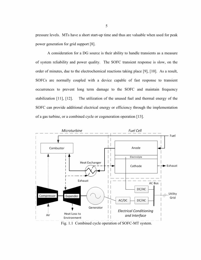
of a gas turbine, or a combined cycle or cogeneration operation [13].

Fig. 1.1 Combined cycle operation of SOFC-MT system.

6

Combined cycle (CC) operation refers to the coupling of heat streams for

purposes within the system itself. For the research of this thesis, CC operations refer to

the coupling of the MT exhaust gas stream and the unused SOFC fuel stream from the

anode channel, as shown in Fig.1.1. Such an implementation of CC operation is typical

in SOFC/MT systems, utilizing the unused exhaust from the MT in a heat recovery

operation to preheat the fuel into the MT to increase efficiency. CC operation will be

discussed in further detail in Chapter 3.

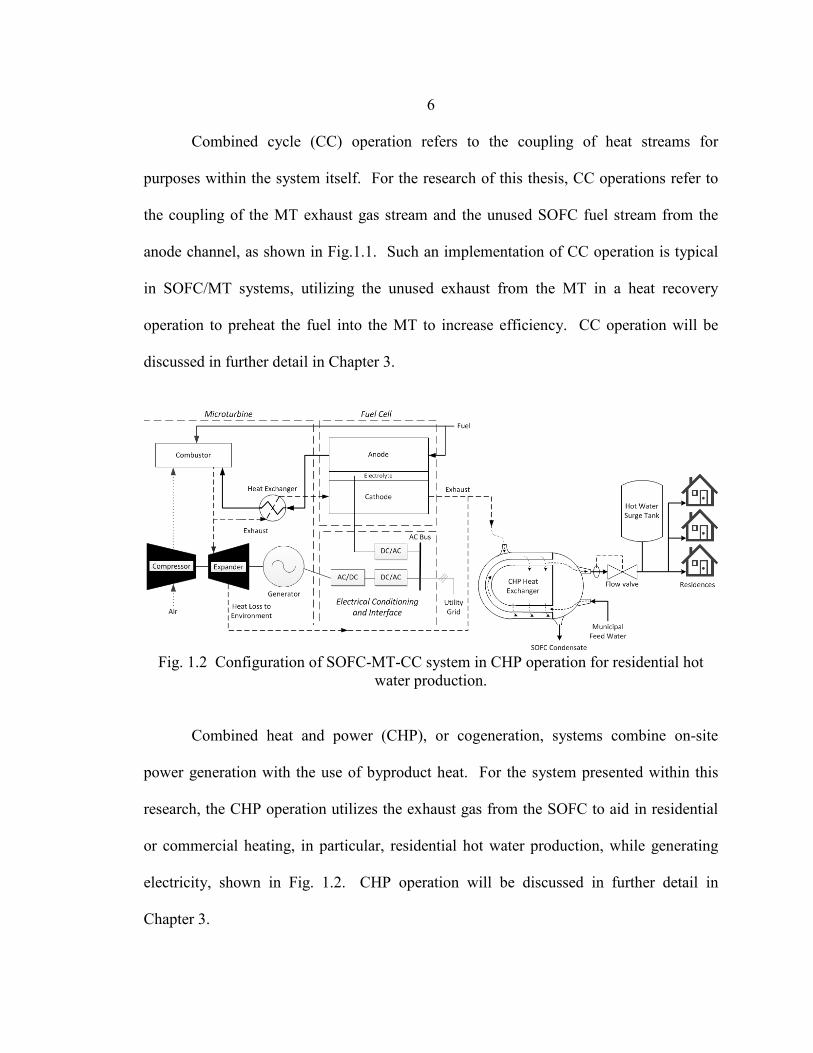
Fig. 1.2 Configuration of SOFC-MT-CC system in CHP operation for residential hot

water production. Combined heat and power (CHP), or cogeneration, systems combine on-site

power generation with the use of byproduct heat. For the system presented within this

research, the CHP operation utilizes the exhaust gas from the SOFC to aid in residential

or commercial heating, in particular, residential hot water production, while generating

electricity, shown in Fig. 1.2. CHP operation will be discussed in further detail in

Chapter 3.

7

Hybrid SOFC-MT systems benefit from combined cycle operation by increasing

the efficiency and transient capabilities of the system along with decreasing fuel costs

and emissions [14]. Efficiencies for hybrid SOFC-MT configurations have been shown

to be greater than 60% [12], [15]. Whereas traditional coal-fired and natural gas-

combustion power plants in the United States operate with efficiency ranges from 20-

38% and 30-50%, respectively [16]-[18]. SOFC-MT hybrids have a great potential to

function as effective electricity sources for the future, while more efficient fuels, i.e.

hydrogen, can subsequently be integrated into the SOFC-MT installations, further

improving generation efficiency and lowering associated costs. The hybrid SOFC-MT

generation systems of today can be viewed as an intermediary generation source

providing a cleaner and more efficient alternative to traditional generation methods until

a robust hydrogen supply and distribution economy has been implemented.

Currently, the research on hybrid renewable systems involving fuel cells, PV,

wind power, and microturbines is growing in the area of distributed generation, due to

increased interest in cleaner and cheaper alternative methods of generation, along with a

proliferation of new technologies. The modeling of such a system consisting of a robust

thermodynamic-based SOFC plant with a machine and thermodynamic-based

microturbine, however, has not. Hybrid SOFC-MT systems have been researched with a

transfer function model [19] or thermodynamic model [12], [20], [21], of a gas turbine

but an integrated model has yet to be developed to our knowledge. Machine, or transfer

function, based models of gas turbines are readily available and commonly used [22].

Thermodynamic based models for gas turbines have also been exhaustively investigated

8

over the past 20 years [23]. For the lack of a combined model, the interconnection of a

transfer function and thermodynamic microturbine model is presented within this thesis.

The ability to analyze efficiency of a system based on thermodynamic modeling, e.g.

reduction of fuel, and transfer function modeling, e.g. power generation and management,

led to this research.

Thesis Organization

The research described in this thesis seeks to concentrate on the modeling,

efficiency evaluation, and power management of a hybrid SOFC-MT system in combined

cycle (CC) operation with combined heat and power (CHP) functionality for residential

applications in islanded or grid-connected modes within a microgrid environment.

Chapter two presents the operation, modeling, and simulation of the SOFC, MT,

combustor, and heat exchanger components of the system. Chapter three provides the

operation and efficiency evaluation of a hybrid SOFC-MT-CC system. Chapter four

presents the power management of the system during transient occurrences. The thesis

concludes in chapter five with a discussion of the results and recommendations for future

work.

9

SYSTEM OPERATION & MODELS

Solid Oxide Fuel Cell

Fuel cells are energy conversion devices that convert the chemical energy of a

fuel into electrical energy [4]. Solid oxide fuel cells (SOFCs) high operating

temperatures of 600-1000°C allow for fuel reforming within the electrode gas channels,

which facilitates the use of a variety of fuels including hydrogen, natural gas, and

hydrocarbon gases.

SOFC Operation

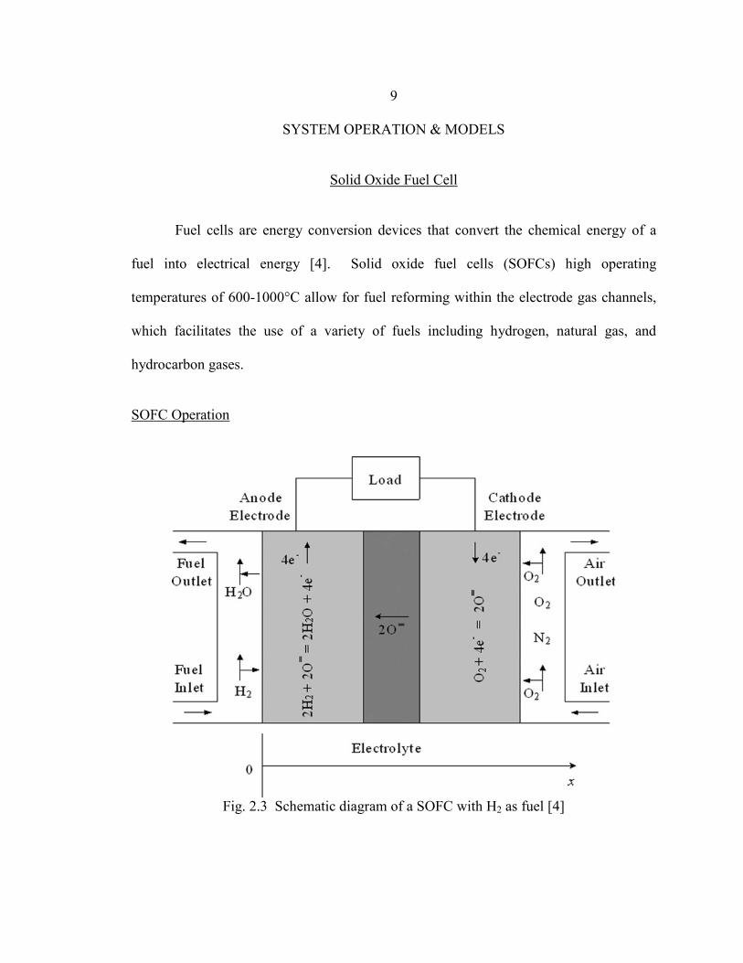
Fig. 2.3 Schematic diagram of a SOFC with H2 as fuel [4]

10

SOFCs operate with a 45-65% efficiency range, and up to 80% in hybrid mode

with CHP systems [13], [24]. The high efficiency of SOFCs is one reason why they

show promise for distributed generation applications [11]. A schematic of a SOFC is

shown in Fig. 2.3 depicting pure hydrogen and atmospheric air as reagents.

At the cathode, oxygen reacts with electrons to form oxygen ions (2.1). The

oxygen ions flow through the electrolyte from cathode to anode. At the anode, the

oxygen ions react with hydrogen to form H2O and excess electrons travel to the external

load (2.2), resulting in an overall reaction producing H2O (2.3).

12

𝑂2 + 2𝑒− → 𝑂2− (2.1)

𝐻2 + 𝑂2− → 𝐻2𝑂 + 𝑒− (2.2)

𝐻2 +12

𝑂2 → 𝐻2𝑂 (2.3)

The chemical reactions when fuel other than hydrogen, such as natural gas (CH4)

is utilized are fundamentally the same with additional intermediate steps, shown in Eq.

(2.4)-(2.7).

𝑂2 + 4𝑒− → 2𝑂2− Cathode (2.4)

𝐻2 + 𝑂2− → 𝐻2𝑂 + 2𝑒− Anode (2.5)

𝐶𝑂 + 𝑂2− → 𝐶𝑂2 + 2𝑒− Anode (2.6)

𝐶𝐻4 + 4𝑂2− → 2𝐻2𝑂 + 𝐶𝑂2 + 8𝑒− Anode (2.7) Since SOFCs are solid-state devices that may employ a ceramic material as the

electrolyte, corrosion and management problems can be significantly curtailed. As

compared to other high operating temperature fuel cells, e.g. molten carbonate fuel cells

11

(MCFCs), which endure higher manufacturing costs and standards due to their

electrolytic material [5].

SOFC Model

A dynamic model for a 5 kW tubular SOFC stack, reported in [4], has been used

in this study for the efficiency evaluation of the SOFC-MT system. The model was

developed based on SOFC electrochemical, thermodynamic, and material diffusion

properties, along with the mass and energy conservation laws with emphasis on the fuel

cell terminal electrical measurements.

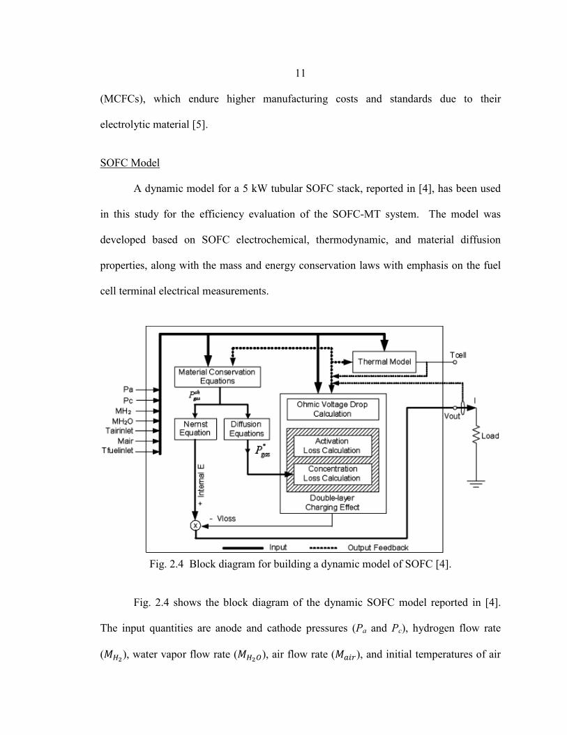
Fig. 2.4 Block diagram for building a dynamic model of SOFC [4].

Fig. 2.4 shows the block diagram of the dynamic SOFC model reported in [4].

The input quantities are anode and cathode pressures (Pa and Pc), hydrogen flow rate

(𝑀𝐻2), water vapor flow rate (𝑀𝐻2𝑂), air flow rate (𝑀𝑎𝑖𝑟), and initial temperatures of air

12

(𝑇𝑎𝑖𝑟 𝑖𝑛𝑙𝑒𝑡) and fuel (𝑇𝑓𝑢𝑒𝑙 𝑖𝑛𝑙𝑒𝑡) of the fuel cell cathode and anode channels, respectively.

At any given load current and time, the cell temperature 𝑇𝑐𝑒𝑙𝑙 is determined and both the

current and temperature are fed back to different blocks, which take part in the

calculation of the SOFC output voltage. The output quantities are the fuel cell voltage

and cell temperature.

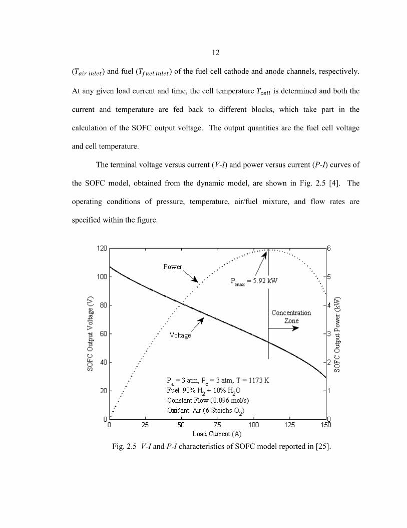
The terminal voltage versus current (V-I) and power versus current (P-I) curves of

the SOFC model, obtained from the dynamic model, are shown in Fig. 2.5 [4]. The

operating conditions of pressure, temperature, air/fuel mixture, and flow rates are

specified within the figure.

Fig. 2.5 V-I and P-I characteristics of SOFC model reported in [25].

13

The activation voltage drop dominates the voltage loss in the low-current region.

As the load current increases, the Ohmic voltage drop increases quickly and is the chief

contributor to the SOFC voltage reduction. When the load current exceeds a certain

value (110 A for the 5 kW model under the given operating conditions), the fuel cell

output voltage will decrease abruptly due to the concentration voltage drop inside the fuel

cell. The concentration voltage drop is a function of current, pressure and temperature.

The effective partial pressures of H2 and O2 are less than those in the electrode channels

while the effective partial pressure of H2O is higher than that in the anode channel. Thus,

the internal voltage of the fuel cell is less than the calculated value. The voltage

difference is referred to as the concentration voltage drop [4].

Model Configuration

The 5 kW stack model consists of 96 individual fuel cells used to generate the

nominal rating. For the purposes of the research in this thesis, the SOFC has a nominal

voltage of 220 V and rated power of 480 kW. To achieve the desired power rating, the 5

kW stack can be interconnected and combined to increase the power. Since the

maximum power is the preferred operating point of each 5 kW stack, it is noted from Fig.

2.3 that the current and voltage corresponding to the maximum power is approximately

110 A at 54 Vdc. However, in order to leave a safe margin so the SOFC stack does not

enter the concentration zone, the operating point is chosen to be 100 A at an output

voltage of 55 Vdc.

A 20 kW module of four 5 kW stacks in series is formed with a nominal output

voltage of 220 Vdc, found by Eq. (2.8) [4].

14

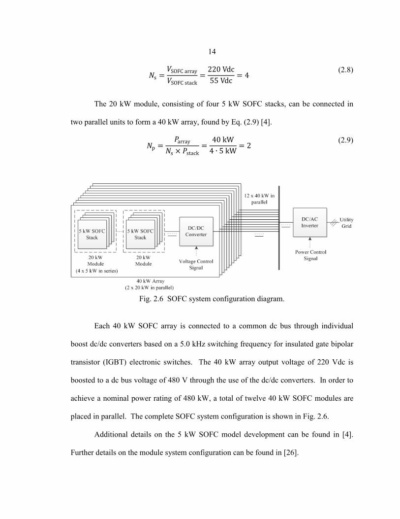
𝑁s =𝑉SOFC array

𝑉SOFC stack=

220 Vdc55 Vdc

= 4 (2.8)

The 20 kW module, consisting of four 5 kW SOFC stacks, can be connected in

two parallel units to form a 40 kW array, found by Eq. (2.9) [4].

𝑁p =𝑃array

𝑁s × 𝑃stack=

40 kW4 ∙ 5 kW

= 2 (2.9)

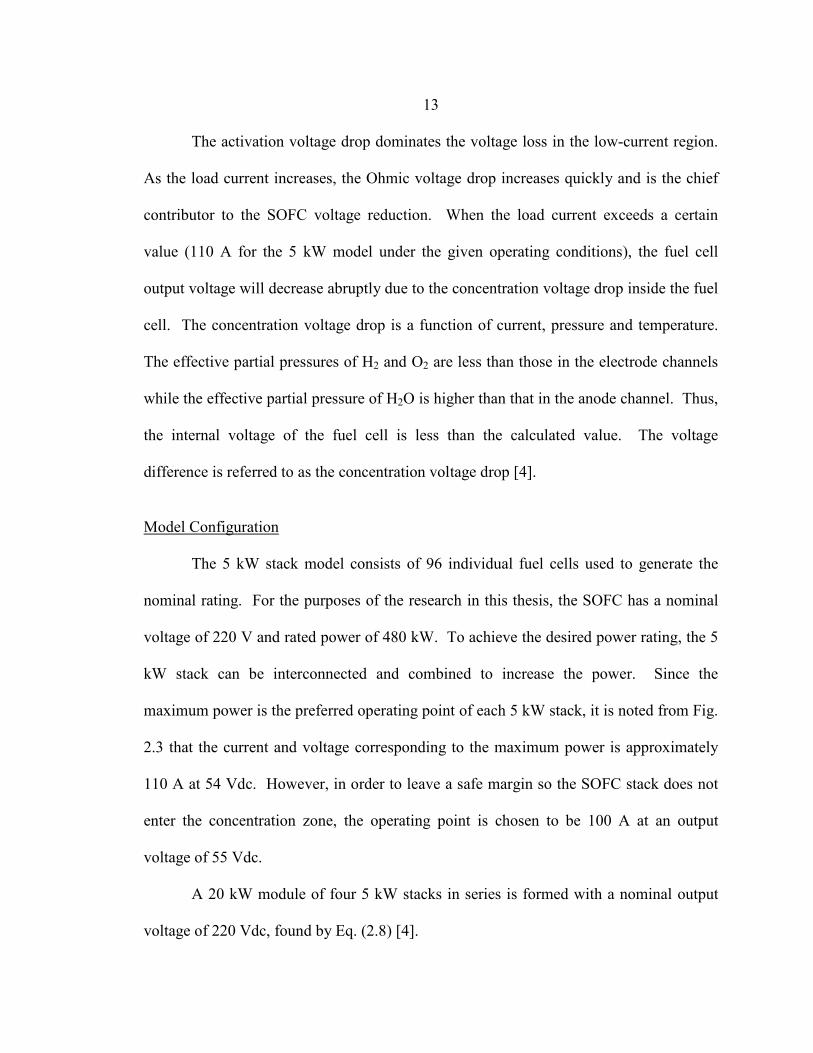
Fig. 2.6 SOFC system configuration diagram.

Each 40 kW SOFC array is connected to a common dc bus through individual

boost dc/dc converters based on a 5.0 kHz switching frequency for insulated gate bipolar

transistor (IGBT) electronic switches. The 40 kW array output voltage of 220 Vdc is

boosted to a dc bus voltage of 480 V through the use of the dc/dc converters. In order to

achieve a nominal power rating of 480 kW, a total of twelve 40 kW SOFC modules are

placed in parallel. The complete SOFC system configuration is shown in Fig. 2.6.

Additional details on the 5 kW SOFC model development can be found in [4].

Further details on the module system configuration can be found in [26].

15

Anode & Cathode Channel Fuel Flow

The steady-state response of the dynamic SOFC model is similar to that reported

in [4] and has been validated by operating data from industry sources. In order to

account for the dynamic behavior of a CC system, the quantity calculations of unused

fuel from the anode channel of the SOFC needed to be implemented. Assuming full

availability of hydrogen fuel and large stoichiometric quantities of water vapor and

oxygen at the cathode, the mass flow rate for H2, H2O and O2 at the inlet and outlet of the

anode and cathode flow channels can be expressed as follows [4]:

𝑀H2in = 𝑀a ∙ 𝜒H2

in = 𝑀a ∙𝑝H2

in

𝑃ach

(2.10a)

𝑀H2out = 𝑀a ∙ 𝜒H2

out = 𝑀a ∙𝑝H2

out

𝑃ach

(2.10b)

𝑀H2Oin = 𝑀a ∙ 𝜒H2O

in = 𝑀a ∙𝑝H2O

in

𝑃ach

(2.11a)

𝑀H2Oout = 𝑀a ∙ 𝜒H2O

out = 𝑀a ∙𝑝H2O

out

𝑃ach

(2.11b)

𝑀O2in = 𝑀c ∙ 𝜒O2

in = 𝑀c ∙𝑝O2

in

𝑃cch

(2.12a)

𝑀O2out = 𝑀c ∙ 𝜒O2

out = 𝑀c ∙𝑝O2

out

𝑃cch

(2.12b)

Where 𝑀𝑖 is the molar flow rate of species i (mol/s), 𝑀𝑎 and 𝑀𝑐 are the molar

flow rates of the anode and cathode channels, respectively (mol/s), 𝜒𝑖 is the mole fraction

of species i, 𝑝𝑖 is the partial pressure of species i (Pa), and 𝑃𝑎 and 𝑃𝑐 are the overall

pressures of the gas mixture in the anode and cathode channels, respectively. The

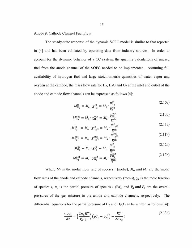
differential equations for the partial pressure of H2 and H2O can be written as follows [4]:

𝑑𝑝H2ch

𝑑𝑡= �

2𝑛𝑎𝑅𝑇𝑉𝑎𝑃a

ch � �𝑝H2in − 𝑝H2

ch � −𝑅𝑇

2𝐹𝑉𝑎𝑖

(2.13a)

16

𝑑𝑝H2Och

𝑑𝑡= �

2𝑛𝑎𝑅𝑇𝑉𝑎𝑃a

ch � �𝑝H2Oin − 𝑝H2O

ch � +𝑅𝑇

2𝐹𝑉𝑎𝑖

(2.13b)

Where R is the gas constant 8.3143 J/(mol K), T the gas temperature (K), 𝑉𝑎 the

volume of the anode channel (m3), and F is Faraday’s constant (96487 C/mol).

The molar flow rate of H2 and H2O out of the anode channel, Eq. (2.10b) and

(2.11b), were implemented in Matlab/Simulink within the existing SOFC model and is a

part of the research presented within this thesis.

For further details concerning the development of the thermodynamic modeling of

the SOFC, the reader is referred to [4].

SOFC Simulation

A simulation of the SOFC model was conducted for the purpose of verifying the

implemented equations of unused fuel from the anode channel. A simulation of the 5 kW

SOFC stack model was conducted over the range of rated input load currents from 0 to

150 A. The simulation parameters for a 5 kW stack model are shown in Table 2.1.

Table 2.1 Simulation Parameters of 5 kW SOFC Stack Model [4]

Parameter Value Fuel flow 0.096 mol/s (90% H2 + 10% H2O) Air flow 0.012 mol/s

Pressures (anode & cathode) 3 atm Initial fuel & air temperature 1173 K

The mass flow rate and the partial pressure of H2 at the outlet of the anode

channel, found via Eq. (2.10a) and (2.13a), is shown to exhibit a correlation. With a

constant mass flow rate of H2 at the inlet of the anode channel over the range of operating

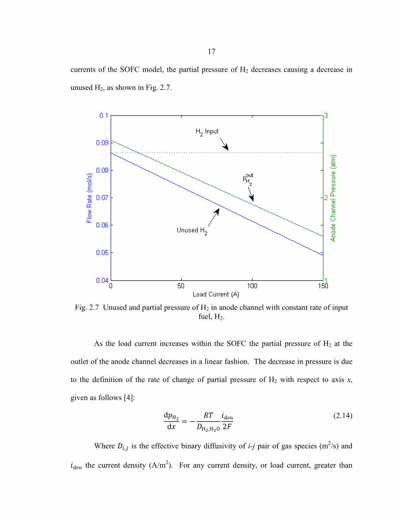
17

currents of the SOFC model, the partial pressure of H2 decreases causing a decrease in

unused H2, as shown in Fig. 2.7.

Fig. 2.7 Unused and partial pressure of H2 in anode channel with constant rate of input

fuel, H2. As the load current increases within the SOFC the partial pressure of H2 at the

outlet of the anode channel decreases in a linear fashion. The decrease in pressure is due

to the definition of the rate of change of partial pressure of H2 with respect to axis x,

given as follows [4]:

d𝑝H2

d𝑥= −

𝑅𝑇𝐷H2,H2O

𝑖den

2𝐹

(2.14)

Where 𝐷𝑖,𝑗 is the effective binary diffusivity of i-j pair of gas species (m2/s) and

𝑖den the current density (A/m2). For any current density, or load current, greater than

18

zero, the rate of change of partial pressure of H2 will be negative. As the load current

increases up to the maximum value of 150 A the partial pressure of H2 will continue to

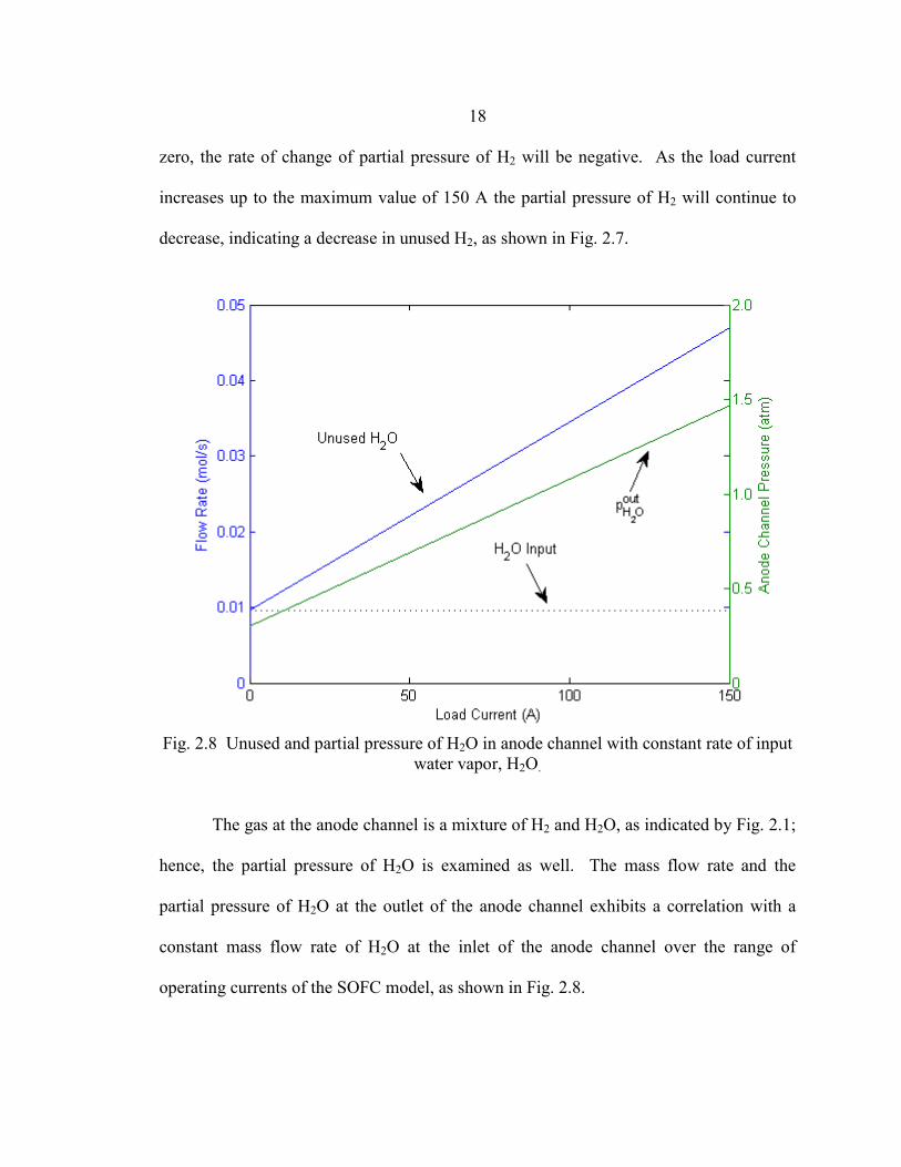
decrease, indicating a decrease in unused H2, as shown in Fig. 2.7.

Fig. 2.8 Unused and partial pressure of H2O in anode channel with constant rate of input

water vapor, H2O. The gas at the anode channel is a mixture of H2 and H2O, as indicated by Fig. 2.1;

hence, the partial pressure of H2O is examined as well. The mass flow rate and the

partial pressure of H2O at the outlet of the anode channel exhibits a correlation with a

constant mass flow rate of H2O at the inlet of the anode channel over the range of

operating currents of the SOFC model, as shown in Fig. 2.8.

19

In a similar fashion as H2, during the increase of load current within the SOFC the

partial pressure of H2O at the outlet of the anode channel increases in a linear fashion.

The increase in pressure is due to the definition of the rate of change of partial pressure of

H2O with respect to axis x, given as follows [4]:

d𝑝H2O

d𝑥=

𝑅𝑇𝐷H2,H2O

𝑖den

2𝐹

(2.15)

For a current density greater than zero, the rate of change of partial pressure of

H2O will be positive, indicating more unused H2O as the load current increases, as

verified by simulation.

The SOFC was also considered for a steady state operation case at a nominal

current of 100 A and rated power of 5 kW; therefore the load current was considered to

ramp up to a constant operating point set to the nominal rating of 100 A at 55 Vdc. The

results of the simulation are shown in the following figures.

Exhibiting the same startup characteristics as previously shown, the amount of

unused H2 along with the partial pressure of H2 in the anode channel decrease as the load

current is increased. Once the SOFC reaches the operating point of 100 A at 55 Vdc, the

mass flow rate and the partial pressure of H2 at the outlet of the anode channel remain

constant, as shown in Fig. 2.9. The molar flow rate and the overall pressure of the gas

mixture in the anode channel, Pa, remain constant throughout the simulation, regardless

of load current. When the load current is constant, the partial pressure of H2 of the anode

channel is constant due to the rate of change equal to zero, as found by Eq. (2.13a).

20

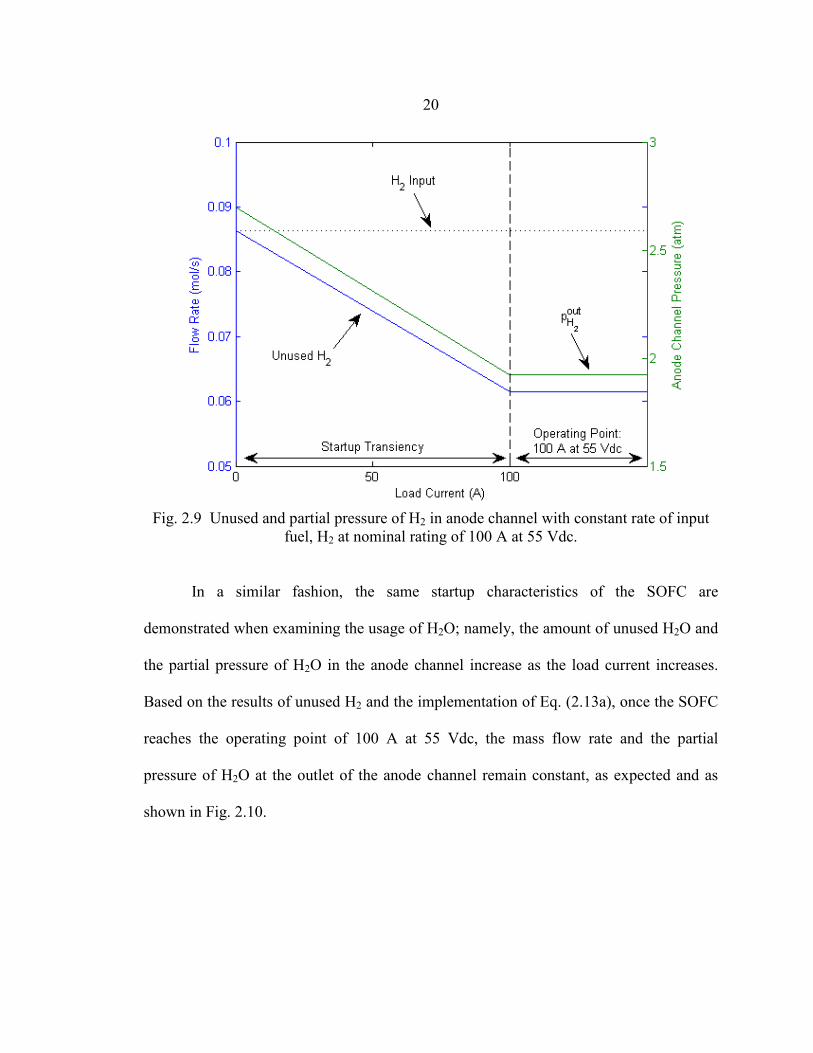
Fig. 2.9 Unused and partial pressure of H2 in anode channel with constant rate of input

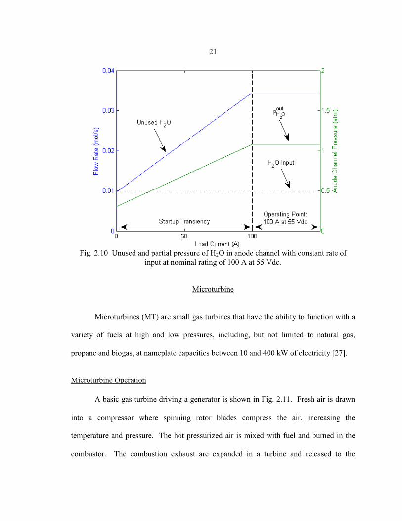
fuel, H2 at nominal rating of 100 A at 55 Vdc. In a similar fashion, the same startup characteristics of the SOFC are

demonstrated when examining the usage of H2O; namely, the amount of unused H2O and

the partial pressure of H2O in the anode channel increase as the load current increases.

Based on the results of unused H2 and the implementation of Eq. (2.13a), once the SOFC

reaches the operating point of 100 A at 55 Vdc, the mass flow rate and the partial

pressure of H2O at the outlet of the anode channel remain constant, as expected and as

shown in Fig. 2.10.

21

Fig. 2.10 Unused and partial pressure of H2O in anode channel with constant rate of

input at nominal rating of 100 A at 55 Vdc.

Microturbine

Microturbines (MT) are small gas turbines that have the ability to function with a

variety of fuels at high and low pressures, including, but not limited to natural gas,

propane and biogas, at nameplate capacities between 10 and 400 kW of electricity [27].

Microturbine Operation

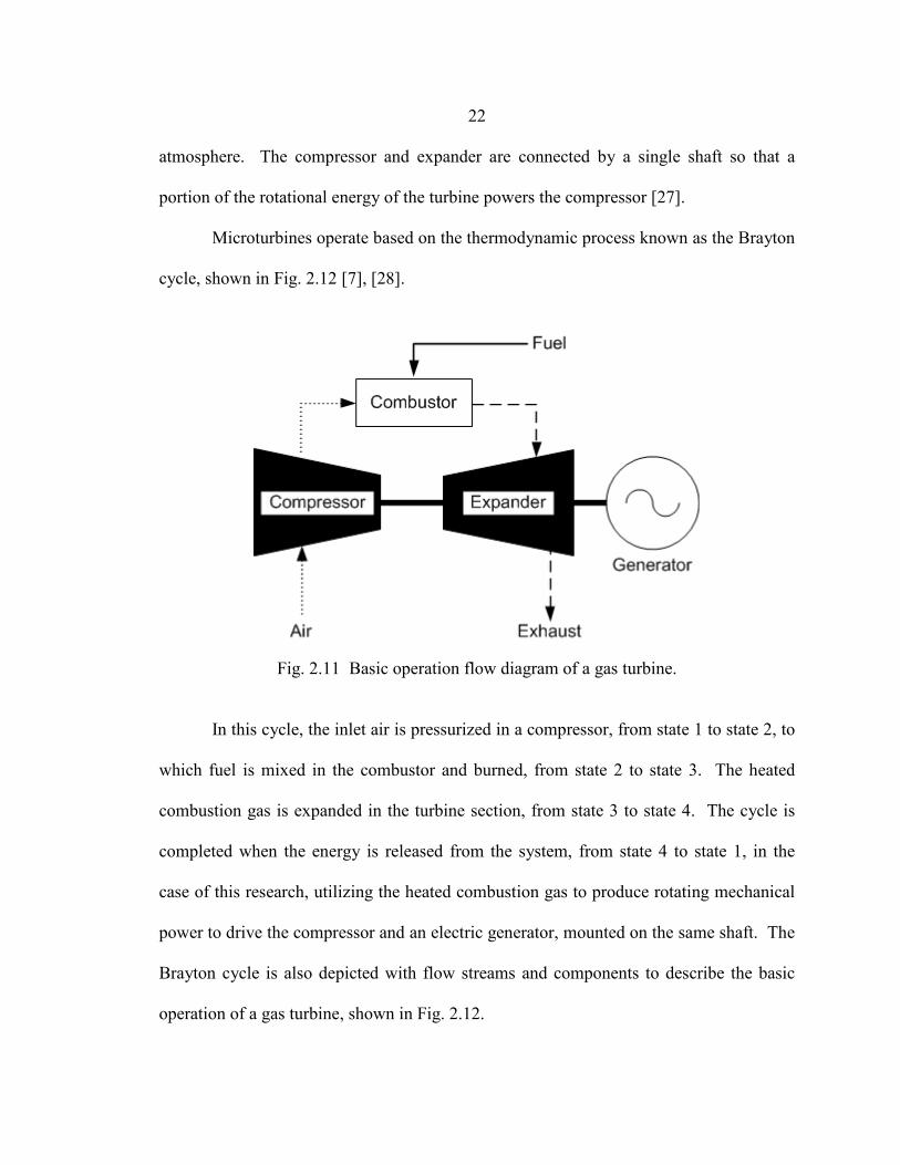
A basic gas turbine driving a generator is shown in Fig. 2.11. Fresh air is drawn

into a compressor where spinning rotor blades compress the air, increasing the

temperature and pressure. The hot pressurized air is mixed with fuel and burned in the

combustor. The combustion exhaust are expanded in a turbine and released to the

22

atmosphere. The compressor and expander are connected by a single shaft so that a

portion of the rotational energy of the turbine powers the compressor [27].

Microturbines operate based on the thermodynamic process known as the Brayton

cycle, shown in Fig. 2.12 [7], [28].

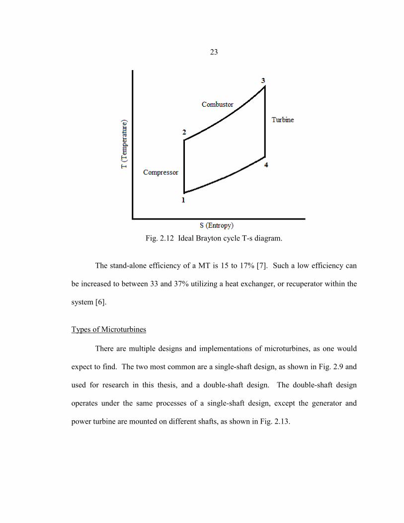
Fig. 2.11 Basic operation flow diagram of a gas turbine. In this cycle, the inlet air is pressurized in a compressor, from state 1 to state 2, to

which fuel is mixed in the combustor and burned, from state 2 to state 3. The heated

combustion gas is expanded in the turbine section, from state 3 to state 4. The cycle is

completed when the energy is released from the system, from state 4 to state 1, in the

case of this research, utilizing the heated combustion gas to produce rotating mechanical

power to drive the compressor and an electric generator, mounted on the same shaft. The

Brayton cycle is also depicted with flow streams and components to describe the basic

operation of a gas turbine, shown in Fig. 2.12.

23

Fig. 2.12 Ideal Brayton cycle T-s diagram.

The stand-alone efficiency of a MT is 15 to 17% [7]. Such a low efficiency can

be increased to between 33 and 37% utilizing a heat exchanger, or recuperator within the

system [6].

Types of Microturbines

There are multiple designs and implementations of microturbines, as one would

expect to find. The two most common are a single-shaft design, as shown in Fig. 2.9 and

used for research in this thesis, and a double-shaft design. The double-shaft design

operates under the same processes of a single-shaft design, except the generator and

power turbine are mounted on different shafts, as shown in Fig. 2.13.

24

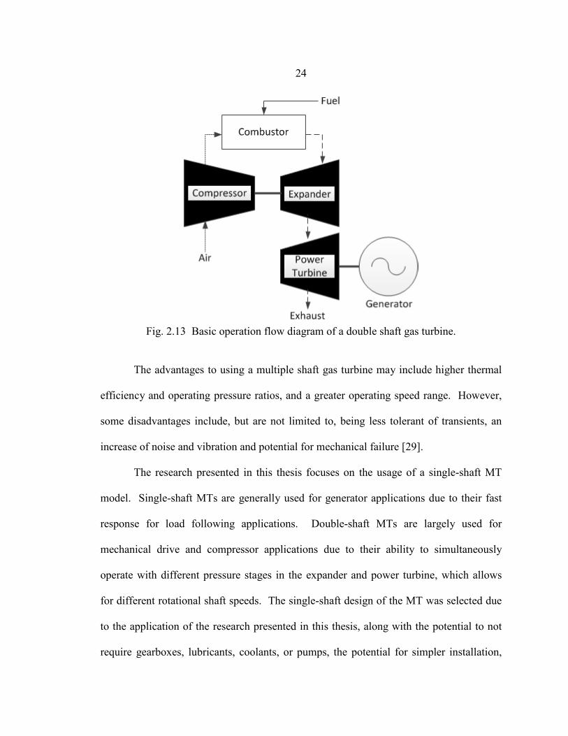
Fig. 2.13 Basic operation flow diagram of a double shaft gas turbine.

The advantages to using a multiple shaft gas turbine may include higher thermal

efficiency and operating pressure ratios, and a greater operating speed range. However,

some disadvantages include, but are not limited to, being less tolerant of transients, an

increase of noise and vibration and potential for mechanical failure [29].

The research presented in this thesis focuses on the usage of a single-shaft MT

model. Single-shaft MTs are generally used for generator applications due to their fast

response for load following applications. Double-shaft MTs are largely used for

mechanical drive and compressor applications due to their ability to simultaneously

operate with different pressure stages in the expander and power turbine, which allows

for different rotational shaft speeds. The single-shaft design of the MT was selected due

to the application of the research presented in this thesis, along with the potential to not

require gearboxes, lubricants, coolants, or pumps, the potential for simpler installation,

25

higher reliability, reduced noise and vibration, lower maintenance requirements, lower

emissions, and continuous combustion [6]. In conjunction with the advantages listed, the

single-shaft design was chosen due to the prior validation and usage of the single shaft

model for distributed generation applications [6], [22].

Operational Speed and Frequency of MT

Depending on the output capacity of the MT, the range of rotational speeds varies

from 50,000 to 120,000 rpm, and as a result high operational frequency, which must be

rectified to DC and inverted to 50 or 60 Hz, contingent to the usage [30]. The power

electronics necessary for the rectification and inversion of frequency within the system

have been previously modeled and verified [6], [31]. The implementation of the power

electronics in [6] and [31] have been modified for the purpose of the research presented

in this thesis to include islanded and grid-connected operations within a microgrid

environment.

Microturbine Model Overview

A transfer function model for a per unit gas turbine, developed by [32], along with

a thermodynamic model developed by the author has been used for this research. The

necessity of integrating the two model types is explained in further detail in the following

sections.

Transfer Function Model

The mathematical representation of a microturbine consists of a single-shaft

design, generator driven gas turbine model that includes speed control, temperature

26

control, and a fuel system. This model has been successfully implemented for DG

simulation applications [14], [33].

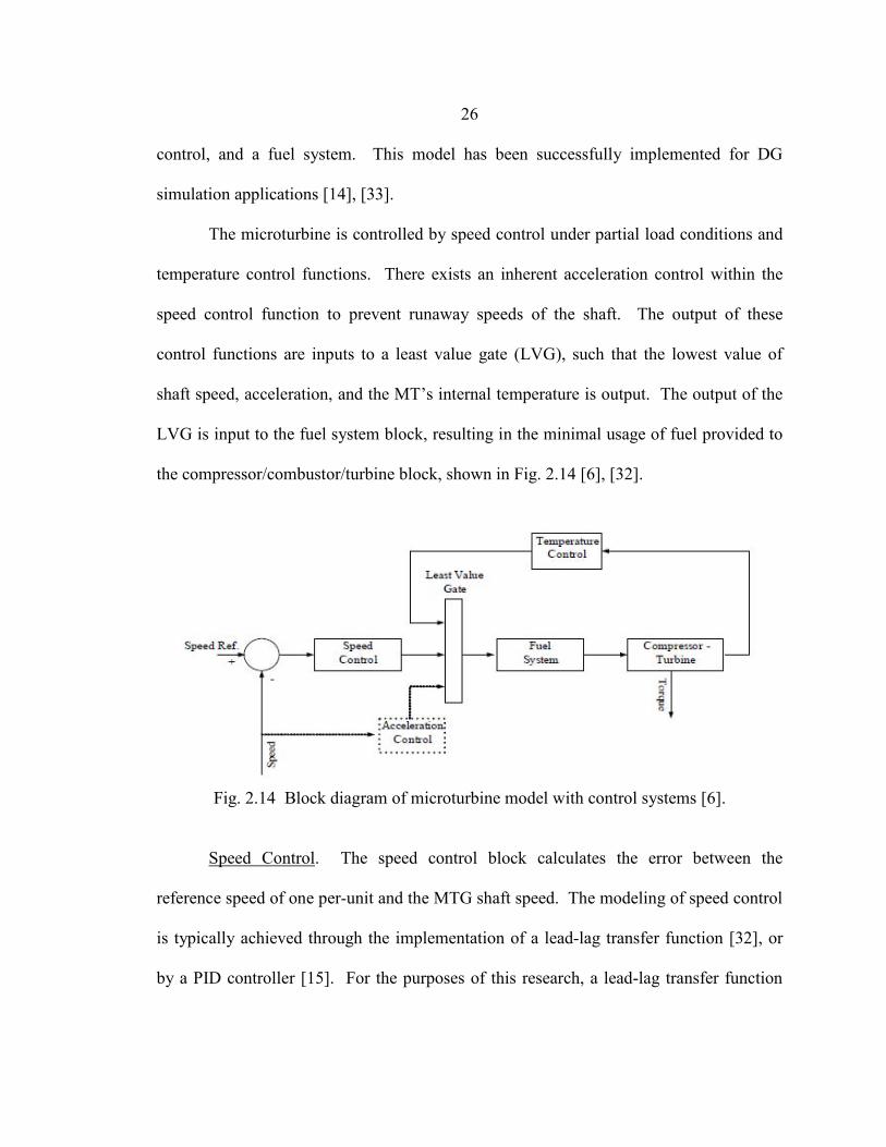
The microturbine is controlled by speed control under partial load conditions and

temperature control functions. There exists an inherent acceleration control within the

speed control function to prevent runaway speeds of the shaft. The output of these

control functions are inputs to a least value gate (LVG), such that the lowest value of

shaft speed, acceleration, and the MT’s internal temperature is output. The output of the

LVG is input to the fuel system block, resulting in the minimal usage of fuel provided to

the compressor/combustor/turbine block, shown in Fig. 2.14 [6], [32].

Fig. 2.14 Block diagram of microturbine model with control systems [6].

Speed Control

[32]

. The speed control block calculates the error between the

reference speed of one per-unit and the MTG shaft speed. The modeling of speed control

is typically achieved through the implementation of a lead-lag transfer function , or

by a PID controller [15]. For the purposes of this research, a lead-lag transfer function

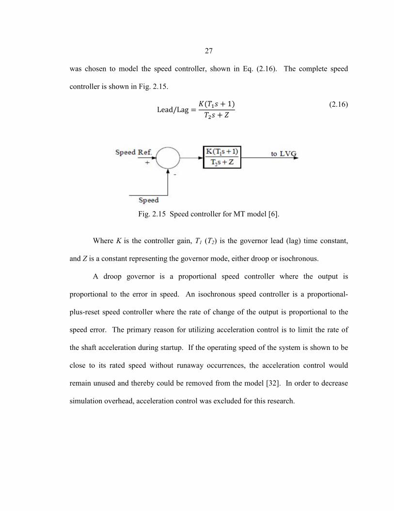
27

was chosen to model the speed controller, shown in Eq. (2.16). The complete speed

controller is shown in Fig. 2.15.

Lead/Lag =𝐾(𝑇1𝑠 + 1)

𝑇2𝑠 + 𝑍

(2.16)

Fig. 2.15 Speed controller for MT model [6].

Where K is the controller gain, T1 (T2) is the governor lead (lag) time constant,

and Z is a constant representing the governor mode, either droop or isochronous.

A droop governor is a proportional speed controller where the output is

proportional to the error in speed. An isochronous speed controller is a proportional-

plus-reset speed controller where the rate of change of the output is proportional to the

speed error. The primary reason for utilizing acceleration control is to limit the rate of

the shaft acceleration during startup. If the operating speed of the system is shown to be

close to its rated speed without runaway occurrences, the acceleration control would

remain unused and thereby could be removed from the model [32]. In order to decrease

simulation overhead, acceleration control was excluded for this research.

28

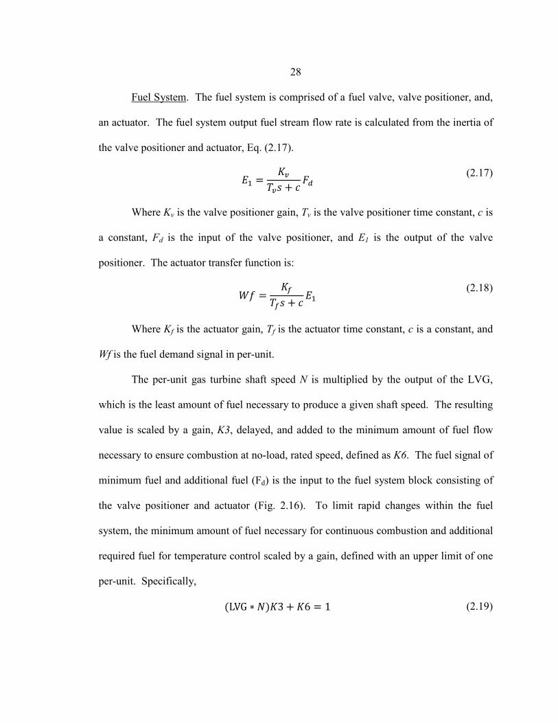
Fuel System

(2.17

. The fuel system is comprised of a fuel valve, valve positioner, and,

an actuator. The fuel system output fuel stream flow rate is calculated from the inertia of

the valve positioner and actuator, Eq. ).

𝐸1 =𝐾𝑣

𝑇𝑣𝑠 + 𝑐𝐹𝑑

(2.17)

Where Kv is the valve positioner gain, Tv is the valve positioner time constant, c is

a constant, Fd is the input of the valve positioner, and E1 is the output of the valve

positioner. The actuator transfer function is:

𝑊𝑓 =𝐾𝑓

𝑇𝑓𝑠 + 𝑐𝐸1

(2.18)

Where Kf is the actuator gain, Tf is the actuator time constant, c is a constant, and

Wf is the fuel demand signal in per-unit.

The per-unit gas turbine shaft speed N is multiplied by the output of the LVG,

which is the least amount of fuel necessary to produce a given shaft speed. The resulting

value is scaled by a gain, K3, delayed, and added to the minimum amount of fuel flow

necessary to ensure combustion at no-load, rated speed, defined as K6. The fuel signal of

minimum fuel and additional fuel (Fd) is the input to the fuel system block consisting of

the valve positioner and actuator (Fig. 2.16). To limit rapid changes within the fuel

system, the minimum amount of fuel necessary for continuous combustion and additional

required fuel for temperature control scaled by a gain, defined with an upper limit of one

per-unit. Specifically,

(LVG ∗ 𝑁)𝐾3 + 𝐾6 = 1 (2.19)

29

Fig. 2.16 Fuel control system for MT model [6].

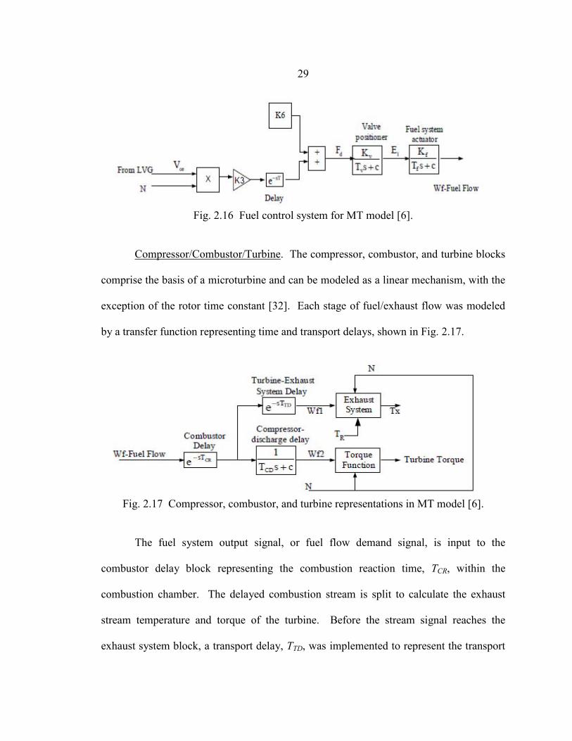
Compressor/Combustor/Turbine

[32]

. The compressor, combustor, and turbine blocks

comprise the basis of a microturbine and can be modeled as a linear mechanism, with the

exception of the rotor time constant . Each stage of fuel/exhaust flow was modeled

by a transfer function representing time and transport delays, shown in Fig. 2.17.

Fig. 2.17 Compressor, combustor, and turbine representations in MT model [6].

The fuel system output signal, or fuel flow demand signal, is input to the

combustor delay block representing the combustion reaction time, TCR, within the

combustion chamber. The delayed combustion stream is split to calculate the exhaust

stream temperature and torque of the turbine. Before the stream signal reaches the

exhaust system block, a transport delay, TTD, was implemented to represent the transport

30

of a stream from the combustion chamber to the expander. In the same manner, prior to

the input of the stream signal to the torque block, a time delay associated with the

compressor discharge, TCD, was implemented.

The exhaust system block calculates the temperature of the exhaust stream, TX

(°F), by the following equation [32]:

𝑇𝑋 = 𝑇𝑅 − 700(1 − 𝑊𝑓1) + 550(1 − 𝑁) (2.20) Where TR is the reference temperature (°F), N is the rotational per-unit shaft speed

of the gas turbine, and Wf1 is the per-unit fuel flow demand signal after passing through

the combustor and transport delay blocks.

The torque block calculates the torque of the gas turbine shaft in per-unit by the

following equation [32]:

Torque = 𝐾𝐻𝐻𝑉(𝑊𝑓2 − 0.23) + 0.5(1 − 𝑁) (2.21) Where KHHV is the higher heating value coefficient of the gas stream in the

combustion chamber and Wf2 is the fuel flow demand signal after passing through the

combustion and compressor discharge delay blocks. The value of KHHV and the constant

0.23 originate from the linearity of the typical power/fuel flow rate characteristics of a

gas turbine; namely, at zero power the fuel rate is 23% and at rated power the fuel rate is

100% [32], [34].

Temperature Control. The temperature control block limits the gas turbine output

power at a given operating setpoint (or reference) temperature of the gas turbine,

independent of ambient temperature, as shown in Fig. 2.18. An air/fuel mixture is burned

in the combustor, resulting in an exhaust stream at increased pressure and temperature to

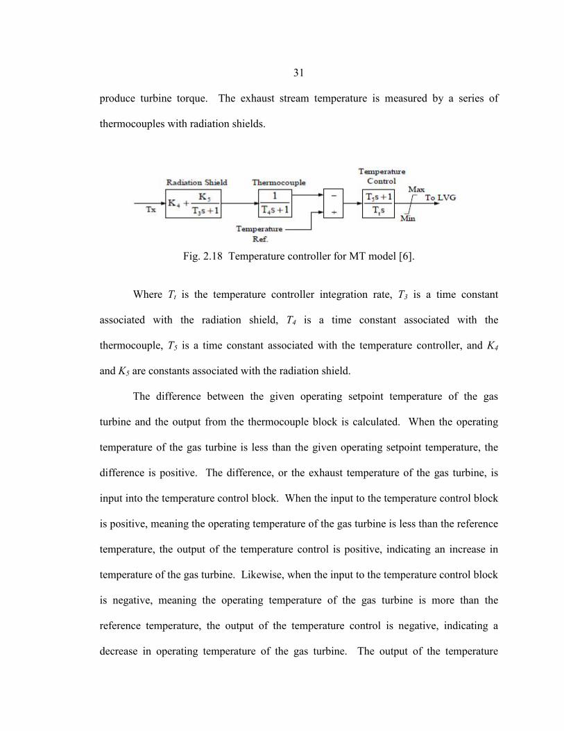
31

produce turbine torque. The exhaust stream temperature is measured by a series of

thermocouples with radiation shields.

Fig. 2.18 Temperature controller for MT model [6].

Where Tt is the temperature controller integration rate, T3 is a time constant

associated with the radiation shield, T4 is a time constant associated with the

thermocouple, T5 is a time constant associated with the temperature controller, and K4

and K5 are constants associated with the radiation shield.

The difference between the given operating setpoint temperature of the gas

turbine and the output from the thermocouple block is calculated. When the operating

temperature of the gas turbine is less than the given operating setpoint temperature, the

difference is positive. The difference, or the exhaust temperature of the gas turbine, is

input into the temperature control block. When the input to the temperature control block

is positive, meaning the operating temperature of the gas turbine is less than the reference

temperature, the output of the temperature control is positive, indicating an increase in

temperature of the gas turbine. Likewise, when the input to the temperature control block

is negative, meaning the operating temperature of the gas turbine is more than the

reference temperature, the output of the temperature control is negative, indicating a

decrease in operating temperature of the gas turbine. The output of the temperature

32

control block is the temperature control signal and the input to the LVG. When the

temperature control signal becomes less than the speed control signal, the gas turbine will

operate on temperature control instead of speed control.

Since the rest of the work completed by the author was developed with actual, not

per-unit, units and temperature in units of Kelvin, the gas turbine model temperatures

were converted to Kelvin for all outputs from the gas turbine block and to Fahrenheit for

all inputs to the gas turbine block. The outputs of the transfer function model are turbine

torque (pu), fuel demand (pu) and exhaust temperature (°F and K). As the SOFC, heat

exchanger, and combustor models are based on thermodynamic principles, the fuel and

air flow rates of the MT were required. In order to calculate the amount of fuel and air

necessary for a given rated power, a thermodynamic model was created and integrated

into the existing model.

Thermodynamic Model

Since the transfer function model of the MT lacks thermodynamic calculations, as

present elsewhere in the system, a limited thermodynamic model was constructed. The

model constructed is limited in that it merely acts as a bridge between the transfer

function model of the MT and the thermodynamic energy flows necessary for the

remaining system.

In order to maintain an accurate yet non-complex model, it is assumed that the

mass flow into the MT is equivalent to the mass flow out of the MT. The mass flow

stream in was assumed to consist of a fuel stream and air stream, shown in Eq. (2.22).

�̇�𝑜𝑢𝑡 = �̇�𝑖𝑛 = �̇�𝑎𝑖𝑟 + �̇�𝑓𝑢𝑒𝑙 (2.22)

33

Since air is comprised of approximately 78% N2 and 20.9% O2 with the remaining

percentage consisting of trace amounts of other gases, the trace gases are neglected from

the calculations. For the purposes of this research, air is assumed to consist of 79% N2

and 21% O2.

The air to fuel ratio (AFR) must be calculated in order to maintain continuous

combustion. Although air consists of N2 and O2, the reactants of the combustion reaction

only rely on O2. For this reason, the AFR is based on mass ratios of the O2 to fuel. The

AFR ratio is calculated to be 3.989, shown in Eq. (2.23).

𝑚𝑎𝑖𝑟

𝑚𝑓𝑢𝑒𝑙=

2𝑚𝑂2

𝑚𝐶𝐻4

=2 ∙ 32 𝑔

𝑚𝑜𝑙16.0425 𝑔

𝑚𝑜𝑙= 3.989

(2.23)

This result indicates a necessary ratio of O2 to CH4 at 3.989. As atmospheric air

is comprised of 21% O2 for the purposes of this research, it follows that the AFR needs to

account for the composition of air. The modification for atmospheric air flow was

calculated to be 18.9952:1 AFR, as shown in Eq. (2.24).

2𝑚𝑂2

𝑚𝐶𝐻4

= 3.989 ⇒𝑚𝑎𝑖𝑟

𝑚𝑓𝑢𝑒𝑙=

3.9890.21

= 18.9952 ≈ 19 (2.24)

For the research within this thesis, the calculated AFR of 18.9952:1 is defined as

19:1. This slightly increased AFR indicates the mixture will be fuel lean, or contain more

air than fuel.

The interconnection between the transfer function model of the MT and the

remainder of the model is required in terms of fuel flow rate due to the lack of other

available rates within the transfer function model. The other flows, namely the air flow,

are then extrapolated based on the previously calculated AFR. Since the air flow has

34

been written in terms of fuel flow as defined by the AFR, it remains to define the oxidant

in terms of fuel as well. The mass of the oxidant, atmospheric air, has been defined as

79% N2 and 21% O2 and can be written as

𝑚𝑎𝑖𝑟 = 0.79 𝑚𝑁2 + 0.21 𝑚𝑂2 �𝑔

𝑚𝑜𝑙� (2.25)

Where 𝑚𝑁2 is 28 g/mol and 𝑚𝑂2 is 32 g/mol. In order to get the mass of air in

terms of oxidant only, Eq. (2.25) was multiplied by one in terms of the mass of O2,

shown in Eq. (2.26).

𝑚𝑎𝑖𝑟 = �0.79 𝑚𝑁2 + 0.21 𝑚𝑂2�0.21 𝑚𝑂2

0.21 𝑚𝑂2

(2.26)

= 0.79 𝑚𝑁2 �0.21 𝑚𝑂2

0.21 𝑚𝑂2

� + 0.21 𝑚𝑂2

= �0.79 𝑚𝑁2

0.21 𝑚𝑂2

� 0.21 𝑚𝑂2 + 0.21 𝑚𝑂2 �𝑔

𝑚𝑜𝑙�

By substituting the molar masses of N2 and O2, rearranging and combining the

mass of O2 terms, Eq. (2.27) is obtained.

𝑚𝑎𝑖𝑟 = �0.79 × 28 𝑔

𝑚𝑜𝑙0.21 × 32 𝑔

𝑚𝑜𝑙 � 0.21 𝑚𝑂2 + 0.21 𝑚𝑂2

(2.27)

= (3.2917)0.21 𝑚𝑂2 + 0.21 𝑚𝑂2

= (4.2917)�0.21 𝑚𝑂2� Based on this result the mass of atmospheric air was found to be approximately

28.8402 g/mol when using the rounded value of 4.2917, shown in Eq. (2.28).

𝑚𝑎𝑖𝑟 = (4.2917)�0.21 𝑚𝑂2� (2.28)

= 4.2917 × 0.21 × 32𝑔

𝑚𝑜𝑙

= 28.8402𝑔

𝑚𝑜𝑙

35

To verify this result, the molecular mass of air was calculated by using the

definition of the composition of air, Eq. (2.25), as shown in Eq. (2.29).

𝑚𝑎𝑖𝑟 = 0.79 𝑚𝑁2 + 0.21 𝑚𝑂2 (2.29)

= 0.79 × 28𝑔

𝑚𝑜𝑙+ 0.21 × 32

𝑔𝑚𝑜𝑙

= 28.8400𝑔

𝑚𝑜𝑙

The error of 0.0002 g/mol is acceptable for the purposes of the research presented

in this thesis and stems from rounding errors. Combining the results of Eq. (2.27) and the

assumed AFR of 19:1, the oxidant of the combustion reaction, O2, can be written in terms

of proportional fuel consumption by setting the two equations equal to each other based

on their equivalence to the value of molecular mass of atmospheric air. The derivation

can be shown in the following manner [35]:

AFR: 𝑚𝑎𝑖𝑟 = 19 𝑚𝑓𝑢𝑒𝑙 Eq. (2.27): 𝑚𝑎𝑖𝑟 = 4.2917 𝑚𝑂2

⇒ 𝑚𝑎𝑖𝑟 = 19 𝑚𝑓𝑢𝑒𝑙 = 4.2917 𝑚𝑂2 (2.30a)

⇒ 𝑚𝑂2 =19

4.2917𝑚𝑓𝑢𝑒𝑙

(2.30b)

The AFR of 19:1 can be substituted into Eq. (2.22) to attain a value of mass flow

in and mass flow out in terms of fuel flow, shown in Eq. (2.31).

�̇�𝑜𝑢𝑡 = �̇�𝑖𝑛 = �̇�𝑎𝑖𝑟 + �̇�𝑓𝑢𝑒𝑙 (2.31) = 19 �̇�𝑓𝑢𝑒𝑙 + �̇�𝑓𝑢𝑒𝑙

= 20 �̇�𝑓𝑢𝑒𝑙 The relationship defined by Eq. (2.31) states that the mass flow in and out of the

combustion chamber of the MT can be written as the fuel flow multiplied by 20.

In order to ultimately determine the amount of fuel necessary to produce a given

amount of power within the MT combustor, the energy flow of the MT combustor must

36

be found. The heat energy produced from a chemical reaction can be described in terms

of enthalpy by the following general thermodynamic relationship [28], [35]:

Heat Energy = �� 𝐻𝑝𝑟𝑜𝑑𝑢𝑐𝑡𝑠� �̇�𝑜𝑢𝑡 − �� 𝐻𝑟𝑒𝑎𝑐𝑡𝑎𝑛𝑡𝑠� �̇�𝑖𝑛 (2.32)

The energy from heat of the products (CO2, H2O) and reactants (CH4, O2) when

CH4 is used as a primary fuel for combustion can be written based on their stoichiometric

quantities

� 𝐻𝑝𝑟𝑜𝑑𝑢𝑐𝑡𝑠 = ∆𝐻𝐶𝑂2 + 2 ∙ ∆𝐻𝐻2𝑂 (2.33)

� 𝐻𝑟𝑒𝑎𝑐𝑡𝑎𝑛𝑡𝑠 = ∆𝐻𝐶𝐻4 + 2 ∙ ∆𝐻𝑂2 (2.34)

The generic enthalpy equation, shown in Eq. (2.32), can be written in terms of

actual products (CO2, H2O) and reactants (CH4, O2), shown in Eq. (2.35).

Heat Energy = �∆𝐻𝐶𝑂2 + 2 ∙ ∆𝐻𝐻2𝑂��̇�𝑜𝑢𝑡 − �∆𝐻𝐶𝐻4 + 2 ∙ ∆𝐻𝑂2��̇�𝑖𝑛 (2.35)

= �∆𝐻𝐶𝑂2 + 2 ∙ ∆𝐻𝐻2𝑂��̇�𝑜𝑢𝑡 − ∆𝐻𝐶𝐻4�̇�𝑓𝑢𝑒𝑙 − 2 ∙ ∆𝐻𝑂2�̇�𝑂2 Since the mass flow out of the MT combustor and the mass flow of oxidant have

been derived in terms of mass flow of fuel, the energy within the combustion reaction can

be written in terms of fuel flow as well, shown in Eq. (2.36).

Heat Energy = �∆𝐻𝐶𝑂2 + 2 ∙ ∆𝐻𝐻2𝑂��20 �̇�𝑓𝑢𝑒𝑙� − ∆𝐻𝐶𝐻4�̇�𝑓𝑢𝑒𝑙

−2 ∙ ∆𝐻𝑂2 �19

4.2917�̇�𝑓𝑢𝑒𝑙�

(2.36)

The fuel flow term can then be factored:

Heat Energy = �̇�𝑓𝑢𝑒𝑙 �20 ∙ ∆𝐻𝐶𝑂2 + 40 ∙ ∆𝐻𝐻2𝑂 − ∆𝐻𝐶𝐻4 − �38

4.2917� ∙ ∆𝐻𝑂2�

(2.37)

Rearranging and solving for fuel flow:

37

�̇�𝑓𝑢𝑒𝑙 =Heat Energy

20 ∙ ∆𝐻𝐶𝑂2 + 40 ∙ ∆𝐻𝐻2𝑂 − ∆𝐻𝐶𝐻4 − � 384.2917� ∙ ∆𝐻𝑂2

(2.38)

Based on the result found in Eq. (2.38), given an amount of heat energy necessary

for a desired amount of power, and by calculating the enthalpy of the combustion

reaction for the products and reactants, the fuel flow rate corresponding to the desired

amount of power can be calculated.

There are many methods to calculate the enthalpy of a reaction [28]; however, the

method used for the research within this thesis utilized the Shomate equation for standard

enthalpy, as defined by [36]. In order to account for the varying temperatures, the

standard enthalpy equation is defined as

𝐻𝑜 − 𝐻298.15𝑜 = 𝐴𝑡 +

𝐵𝑡2

2+

𝐶𝑡3

3+

𝐷𝑡4

4−

𝐸𝑡

+ 𝐹 − 𝐻 (2.39)

Where 𝐻𝑜 is the standard enthalpy, 𝐻298.15

𝑜 is the standard enthalpy at 298.15 K, t

is the operating temperature of the species (K), A, B, C, D, E, F, H are the Shomate

equation parameters for thermochemical functions and differ by chemical species and

temperature ranges [36].

MT Simulation

The thermodynamic model of the MT was implemented within the

Matlab/Simulink environment. A simulation of the MT at a rated power of 250 kW was

conducted for the purpose of verifying the implemented equations of operating

temperature, thermodynamic heat flow, fuel flow, and power calculations. The

configuration of the simulation is shown in Fig. 2.19. The simulation parameters for a

MT per-unit and thermodynamic models are shown in Table 2.2.

38

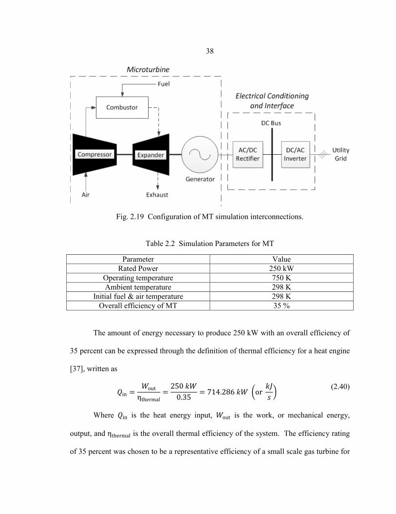
Fig. 2.19 Configuration of MT simulation interconnections.

Table 2.2 Simulation Parameters for MT

Parameter Value Rated Power 250 kW

Operating temperature 750 K Ambient temperature 298 K

Initial fuel & air temperature 298 K Overall efficiency of MT 35 %

The amount of energy necessary to produce 250 kW with an overall efficiency of

35 percent can be expressed through the definition of thermal efficiency for a heat engine

[37], written as

𝑄in =𝑊out

ηthermal=

250 𝑘𝑊0.35

= 714.286 𝑘𝑊 �or 𝑘𝐽𝑠

� (2.40)

Where 𝑄in is the heat energy input, 𝑊out is the work, or mechanical energy,

output, and ηthermal is the overall thermal efficiency of the system. The efficiency rating

of 35 percent was chosen to be a representative efficiency of a small scale gas turbine for

39

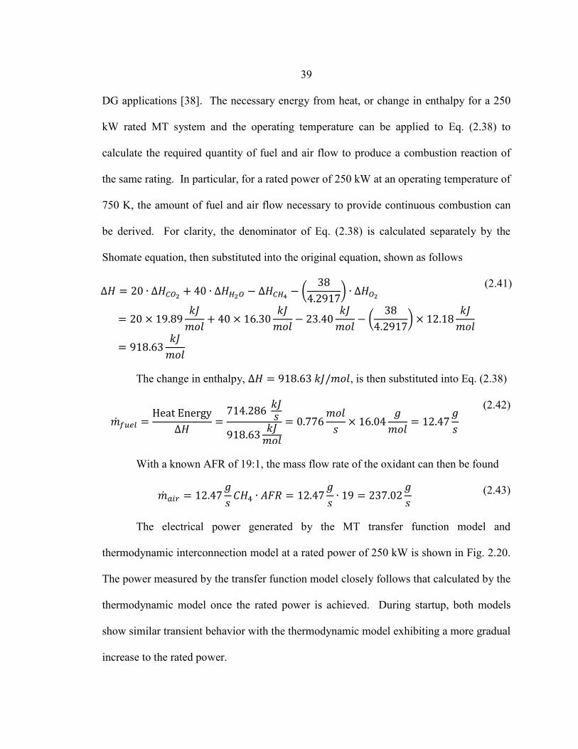
DG applications [38]. The necessary energy from heat, or change in enthalpy for a 250

kW rated MT system and the operating temperature can be applied to Eq. (2.38) to

calculate the required quantity of fuel and air flow to produce a combustion reaction of

the same rating. In particular, for a rated power of 250 kW at an operating temperature of

750 K, the amount of fuel and air flow necessary to provide continuous combustion can

be derived. For clarity, the denominator of Eq. (2.38) is calculated separately by the

Shomate equation, then substituted into the original equation, shown as follows

Δ𝐻 = 20 ∙ ∆𝐻𝐶𝑂2 + 40 ∙ ∆𝐻𝐻2𝑂 − ∆𝐻𝐶𝐻4 − �38

4.2917� ∙ ∆𝐻𝑂2

= 20 × 19.89𝑘𝐽

𝑚𝑜𝑙+ 40 × 16.30

𝑘𝐽𝑚𝑜𝑙

− 23.40𝑘𝐽

𝑚𝑜𝑙− �

384.2917

� × 12.18𝑘𝐽

𝑚𝑜𝑙

= 918.63𝑘𝐽

𝑚𝑜𝑙

(2.41)

The change in enthalpy, Δ𝐻 = 918.63 𝑘𝐽/𝑚𝑜𝑙, is then substituted into Eq. (2.38)

�̇�𝑓𝑢𝑒𝑙 =Heat Energy

Δ𝐻=

714.286 𝑘𝐽𝑠

918.63 𝑘𝐽𝑚𝑜𝑙

= 0.776𝑚𝑜𝑙

𝑠× 16.04

𝑔𝑚𝑜𝑙

= 12.47𝑔𝑠

(2.42)

With a known AFR of 19:1, the mass flow rate of the oxidant can then be found

�̇�𝑎𝑖𝑟 = 12.47𝑔𝑠

𝐶𝐻4 ∙ 𝐴𝐹𝑅 = 12.47𝑔𝑠

∙ 19 = 237.02𝑔𝑠

(2.43)

The electrical power generated by the MT transfer function model and

thermodynamic interconnection model at a rated power of 250 kW is shown in Fig. 2.20.

The power measured by the transfer function model closely follows that calculated by the

thermodynamic model once the rated power is achieved. During startup, both models

show similar transient behavior with the thermodynamic model exhibiting a more gradual

increase to the rated power.

40

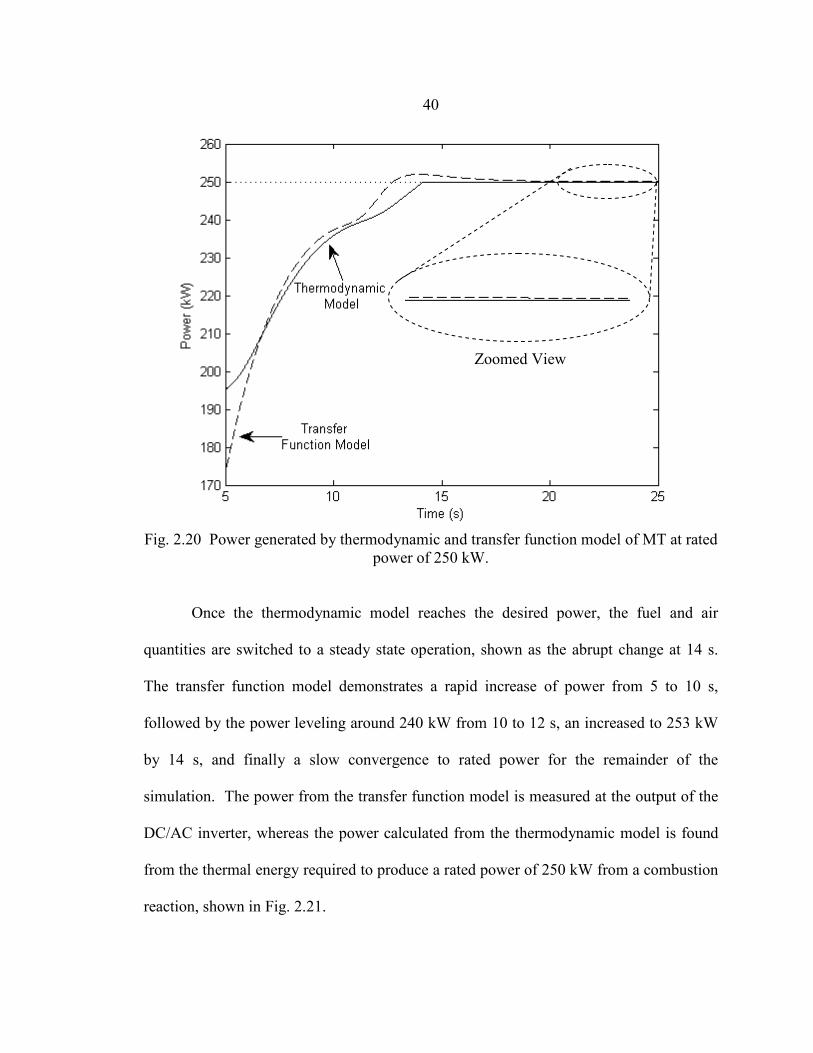
Fig. 2.20 Power generated by thermodynamic and transfer function model of MT at rated

power of 250 kW. Once the thermodynamic model reaches the desired power, the fuel and air

quantities are switched to a steady state operation, shown as the abrupt change at 14 s.

The transfer function model demonstrates a rapid increase of power from 5 to 10 s,

followed by the power leveling around 240 kW from 10 to 12 s, an increased to 253 kW

by 14 s, and finally a slow convergence to rated power for the remainder of the

simulation. The power from the transfer function model is measured at the output of the

DC/AC inverter, whereas the power calculated from the thermodynamic model is found

from the thermal energy required to produce a rated power of 250 kW from a combustion

reaction, shown in Fig. 2.21.

Zoomed View

41

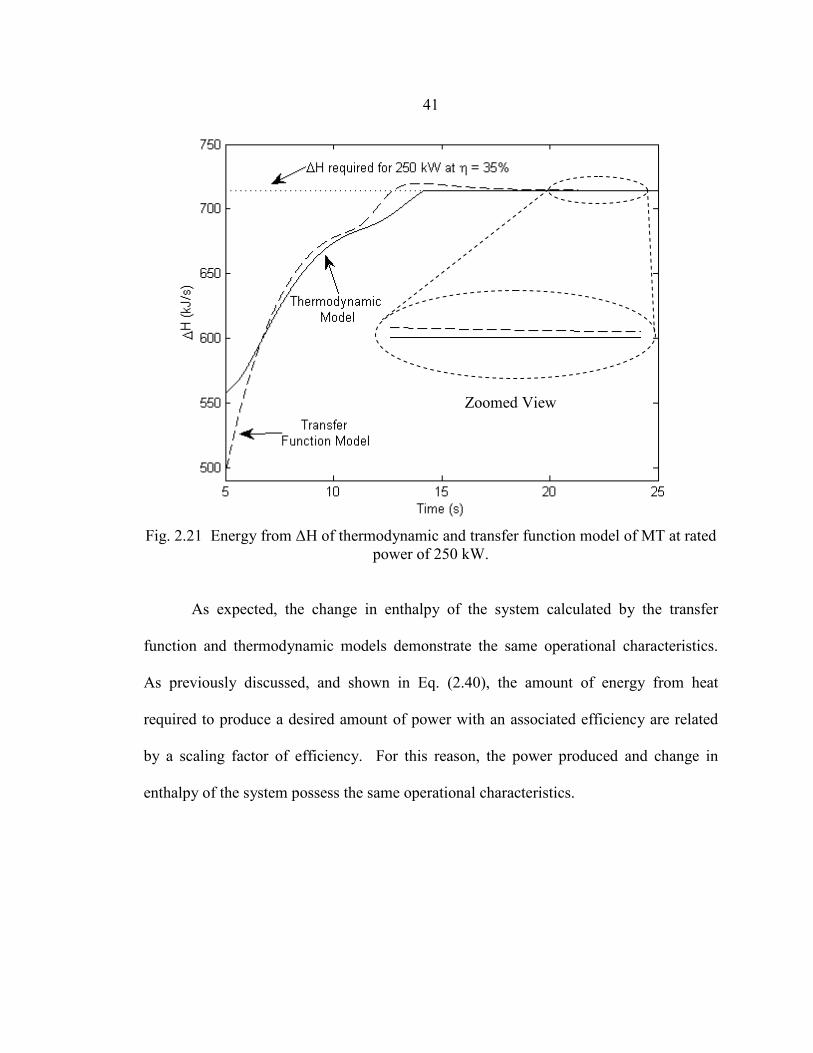
Fig. 2.21 Energy from ΔH of thermodynamic and transfer function model of MT at rated

power of 250 kW. As expected, the change in enthalpy of the system calculated by the transfer

function and thermodynamic models demonstrate the same operational characteristics.

As previously discussed, and shown in Eq. (2.40), the amount of energy from heat

required to produce a desired amount of power with an associated efficiency are related

by a scaling factor of efficiency. For this reason, the power produced and change in

enthalpy of the system possess the same operational characteristics.

Zoomed View

42

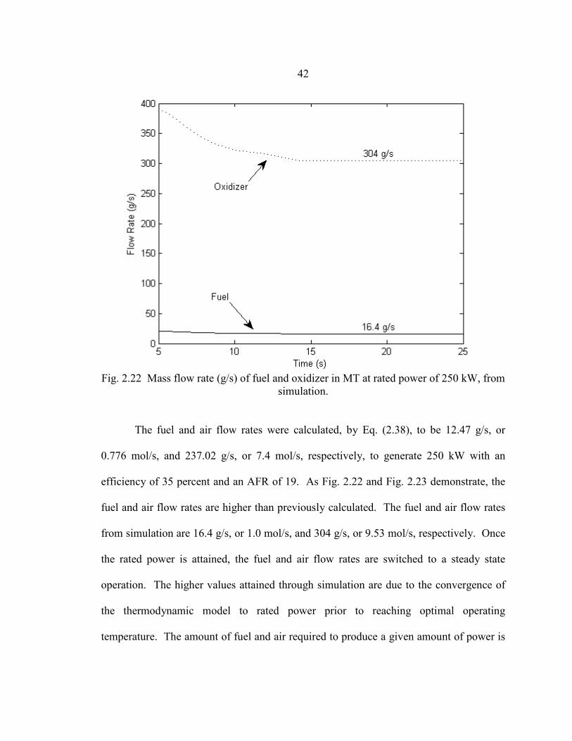
Fig. 2.22 Mass flow rate (g/s) of fuel and oxidizer in MT at rated power of 250 kW, from

simulation. The fuel and air flow rates were calculated, by Eq. (2.38), to be 12.47 g/s, or

0.776 mol/s, and 237.02 g/s, or 7.4 mol/s, respectively, to generate 250 kW with an

efficiency of 35 percent and an AFR of 19. As Fig. 2.22 and Fig. 2.23 demonstrate, the

fuel and air flow rates are higher than previously calculated. The fuel and air flow rates

from simulation are 16.4 g/s, or 1.0 mol/s, and 304 g/s, or 9.53 mol/s, respectively. Once

the rated power is attained, the fuel and air flow rates are switched to a steady state

operation. The higher values attained through simulation are due to the convergence of

the thermodynamic model to rated power prior to reaching optimal operating

temperature. The amount of fuel and air required to produce a given amount of power is

43

decreased as the operating temperature increases. The heat energy of the reactants

increases with temperature, thus requiring a lower flow rate.

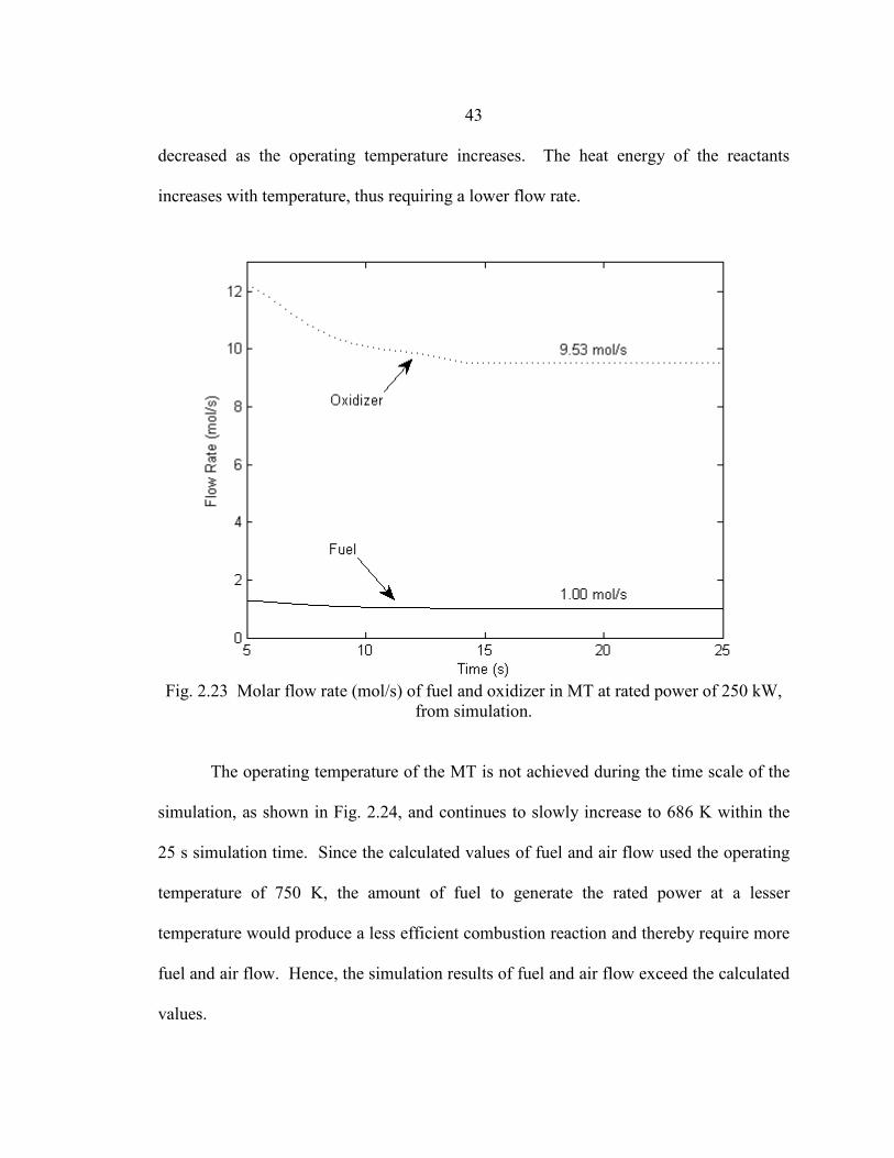
Fig. 2.23 Molar flow rate (mol/s) of fuel and oxidizer in MT at rated power of 250 kW,

from simulation. The operating temperature of the MT is not achieved during the time scale of the

simulation, as shown in Fig. 2.24, and continues to slowly increase to 686 K within the

25 s simulation time. Since the calculated values of fuel and air flow used the operating

temperature of 750 K, the amount of fuel to generate the rated power at a lesser

temperature would produce a less efficient combustion reaction and thereby require more

fuel and air flow. Hence, the simulation results of fuel and air flow exceed the calculated

values.

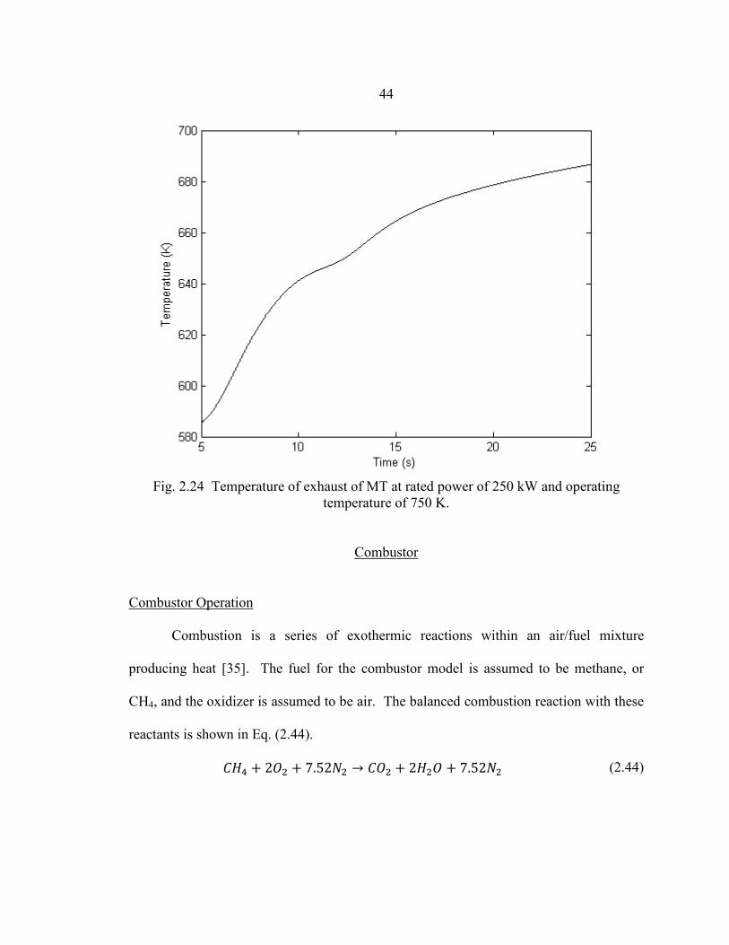
44

Fig. 2.24 Temperature of exhaust of MT at rated power of 250 kW and operating

temperature of 750 K.

Combustor

Combustor Operation

Combustion is a series of exothermic reactions within an air/fuel mixture

producing heat [35]. The fuel for the combustor model is assumed to be methane, or

CH4, and the oxidizer is assumed to be air. The balanced combustion reaction with these

reactants is shown in Eq. (2.44).

𝐶𝐻4 + 2𝑂2 + 7.52𝑁2 → 𝐶𝑂2 + 2𝐻2𝑂 + 7.52𝑁2 (2.44)

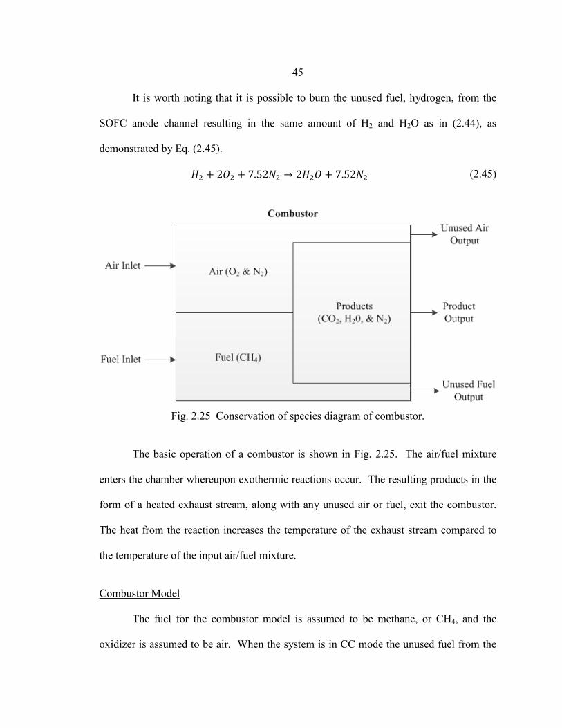
45

It is worth noting that it is possible to burn the unused fuel, hydrogen, from the

SOFC anode channel resulting in the same amount of H2 and H2O as in (2.44), as

demonstrated by Eq. (2.45).

𝐻2 + 2𝑂2 + 7.52𝑁2 → 2𝐻2𝑂 + 7.52𝑁2 (2.45)

Fig. 2.25 Conservation of species diagram of combustor.

The basic operation of a combustor is shown in Fig. 2.25. The air/fuel mixture

enters the chamber whereupon exothermic reactions occur. The resulting products in the

form of a heated exhaust stream, along with any unused air or fuel, exit the combustor.

The heat from the reaction increases the temperature of the exhaust stream compared to

the temperature of the input air/fuel mixture.

Combustor Model

The fuel for the combustor model is assumed to be methane, or CH4, and the

oxidizer is assumed to be air. When the system is in CC mode the unused fuel from the

46

SOFC anode channel is a mixture of H2 and H2O. The model accounts for this change in

fuel, from CH4 to H2, by calculating the enthalpy of an H-O combustion reaction defined

in Eq. (2.45).

Conservation of Chemical Specie

(2.46)

s. Due to the scope of this research a

simplified, or algebraic, but still valid, approach to defining the conservation of chemical

species within the combustion reaction was taken. The ideal mixture equations can be

defined by the mass fractions of each species within the combustion reaction.

Specifically, the ideal mass fraction of the oxidizer (O2 and N2), fuel (CH4), and products

(CO2, H2O, and N2) are defined by the ratios of their respective masses to the total mass

of all species, shown in Eq. -(2.48).

𝑤𝑜𝑥𝑖𝑑𝑖𝑧𝑒𝑟 =𝑀𝑜𝑥𝑖𝑑𝑖𝑧𝑒𝑟

𝑀𝑜𝑥𝑖𝑑𝑖𝑧𝑒𝑟 + 𝑀𝑓𝑢𝑒𝑙 + 𝑀𝑝𝑟𝑜𝑑𝑢𝑐𝑡𝑠

(2.46)

𝑤𝑓𝑢𝑒𝑙 =𝑀𝑓𝑢𝑒𝑙

𝑀𝑜𝑥𝑖𝑑𝑖𝑧𝑒𝑟 + 𝑀𝑓𝑢𝑒𝑙 + 𝑀𝑝𝑟𝑜𝑑𝑢𝑐𝑡𝑠

(2.47)

𝑤𝑝𝑟𝑜𝑑𝑢𝑐𝑡𝑠 =𝑀𝑝𝑟𝑜𝑑𝑢𝑐𝑡𝑠

𝑀𝑜𝑥𝑖𝑑𝑖𝑧𝑒𝑟 + 𝑀𝑓𝑢𝑒𝑙 + 𝑀𝑝𝑟𝑜𝑑𝑢𝑐𝑡𝑠

(2.48)

Where w is the mass fraction of each compound and M is the molar mass of each

compound (g/mol). This conservation can also be demonstrated graphically, as shown in

Fig. 2.25.

Based on the assumption of an ideal mixture of gas, the mass fraction of the

products can be written

𝑤𝑝𝑟𝑜𝑑𝑢𝑐𝑡𝑠 = 1 − 𝑤𝑜𝑥𝑖𝑑𝑖𝑧𝑒𝑟 − 𝑤𝑓𝑢𝑒𝑙 (2.49)

47

As Fig. 2.25 demonstrates, the oxidizer and fuel enter the combustion chamber,

whereupon combustion of the species occurs, resulting in the creation of the product

species. The unused oxidizer and fuel exit the combustor along with the product species.

The conservation of chemical species equations are supplemented by conservation of

mass equations described in the following section.

Conservation of Mass

[35]

. The conservation of mass equations describe the

consumption and production of chemical species based on collision theory of combustion

reactions presented by . During the combustion reaction both the oxidizer and fuel

are consumed. However, the rate at which oxidizer and fuel are consumed depends on

the stoichiometry of the reaction. For this reason, the mass conservation equations have

been written in terms of the oxidizer and fuel, shown in Eq. (2.50), (2.51).

𝑉𝑑𝑤𝑜𝑥𝑖𝑑(𝑡)

𝑑𝑡= �̇�𝑖𝑛𝑤𝑜𝑥𝑖𝑑𝑖𝑛(𝑡) − �̇�𝑜𝑢𝑡𝑤𝑜𝑥𝑖𝑑𝑜𝑢𝑡(𝑡) + 𝑀𝑓𝑢𝑒𝑙𝑘(𝑡)𝑉

𝑤𝑜𝑥𝑖𝑑

𝑤𝑓𝑢𝑒𝑙

(2.50)

𝑉𝑑𝑤𝑓𝑢𝑒𝑙(𝑡)

𝑑𝑡= �̇�𝑖𝑛𝑤𝑓𝑢𝑒𝑙𝑖𝑛(𝑡) − �̇�𝑜𝑢𝑡𝑤𝑓𝑢𝑒𝑙𝑜𝑢𝑡(𝑡) + 𝑀𝑓𝑢𝑒𝑙𝑘(𝑡)𝑉

(2.51)

Where 𝑉 is the volume of the combustor (assumed to be 1 m3), 𝑤𝑜𝑥𝑖𝑑𝑖𝑛and 𝑤𝑓𝑢𝑒𝑙𝑖𝑛

are the mass fraction of oxidizer and fuel into the combustor, 𝑤𝑜𝑥𝑖𝑑𝑜𝑢𝑡 and 𝑤𝑓𝑢𝑒𝑙𝑜𝑢𝑡 are

the mass fraction of oxidizer and fuel out of the combustor, �̇�𝑖𝑛 is the mass flow rate into

the combustor, �̇�𝑜𝑢𝑡 is the mass flow rate out of the combustor, and 𝑘 is the Arrhenius

rate term for consumption of species due to the combustion reaction.

The Arrhenius term is defined for a fuel of CH4 as [35]:

𝑘(𝑡) = �−24100𝑘𝑚𝑜𝑙𝑘𝑔 ∙ 𝑠

� 𝑤𝑓𝑢𝑒𝑙(𝑡)−0.3(0.233𝑤𝑜𝑥𝑖𝑑(𝑡))1.3𝑒−15908

𝑇(𝑡) (2.52)

48

For further detail the Arrhenius form and subsequent calculations of coefficients

for a given species, the reader is directed to [35].

Conservation of Energy

[28]

. The first law of thermodynamics for an open system,

such as a fuel cell or gas turbine, specifies that the rate of change of energy produced by

the system is equivalent to the difference in flow rates in and out of the system. For a

system under constant pressure, the first law can be written, in terms of enthalpy and heat

flow, in the following manner :

𝑑𝑄 − 𝑑𝑊 = � �̇�𝑖∆𝐻𝑖𝑝𝑟𝑜𝑑𝑢𝑐𝑡𝑠

− � �̇�𝑖∆𝐻𝑖𝑟𝑒𝑎𝑐𝑡𝑎𝑛𝑡𝑠

(2.53)

Where dQ is the rate of heat produced within the system (J/s), dW is the rate of

work within the system (J/s), ∆𝐻𝑟𝑒𝑎𝑐𝑡𝑖𝑜𝑛 is the change in enthalpy within the system (J/s),

�̇�𝑖 is the molar flow rate of the input or output stream (mol/s), and 𝐻𝑖 is the specific

enthalpy of the input or output stream (J/mol). Eq. (2.54) is implemented under the

assumption of constant pressure operation written as:

∆𝐻 = 𝑄 = �̇�𝑖𝑐𝑝∆𝑇 (2.54) Where cp is the specific heat capacity of a given compound (J/mol K) and ∆𝑇 is

the change in temperature of the input and output streams (K). The specific gas heat

capacity was calculated using the Shomate equation, as defined by [36]. By definition,

specific heat capacity is the amount of energy required to increase the temperature of a

compound by 1℃, leading to the fact that the specific heat capacity will vary for different

temperatures [28]. In order to account for the varying temperatures, the specific gas heat

capacity equation is defined as [36]

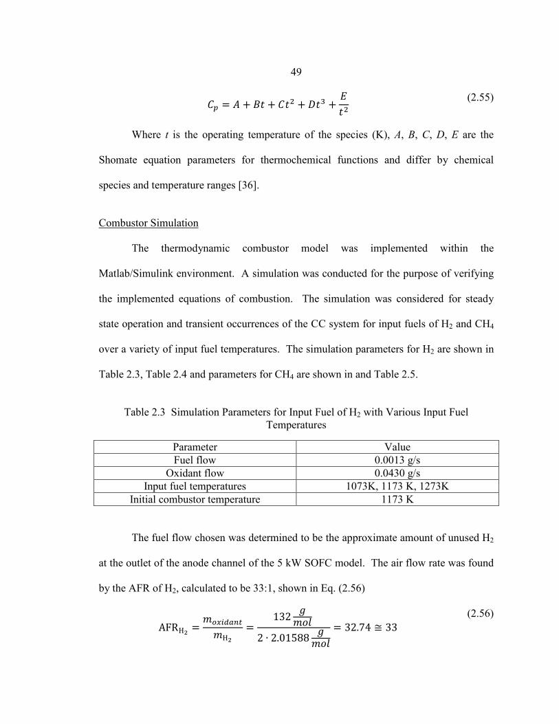
49

𝐶𝑝 = 𝐴 + 𝐵𝑡 + 𝐶𝑡2 + 𝐷𝑡3 +𝐸𝑡2

(2.55)

Where t is the operating temperature of the species (K), A, B, C, D, E are the

Shomate equation parameters for thermochemical functions and differ by chemical

species and temperature ranges [36].

Combustor Simulation

The thermodynamic combustor model was implemented within the

Matlab/Simulink environment. A simulation was conducted for the purpose of verifying

the implemented equations of combustion. The simulation was considered for steady

state operation and transient occurrences of the CC system for input fuels of H2 and CH4

over a variety of input fuel temperatures. The simulation parameters for H2 are shown in

Table 2.3, Table 2.4 and parameters for CH4 are shown in and Table 2.5.

Table 2.3 Simulation Parameters for Input Fuel of H2 with Various Input Fuel

Temperatures

Parameter Value Fuel flow 0.0013 g/s

Oxidant flow 0.0430 g/s Input fuel temperatures 1073K, 1173 K, 1273K

Initial combustor temperature 1173 K

The fuel flow chosen was determined to be the approximate amount of unused H2

at the outlet of the anode channel of the 5 kW SOFC model. The air flow rate was found

by the AFR of H2, calculated to be 33:1, shown in Eq. (2.56)

AFRH2 =𝑚𝑜𝑥𝑖𝑑𝑎𝑛𝑡

𝑚H2

=132 𝑔

𝑚𝑜𝑙

2 ∙ 2.01588 𝑔𝑚𝑜𝑙

= 32.74 ≅ 33 (2.56)

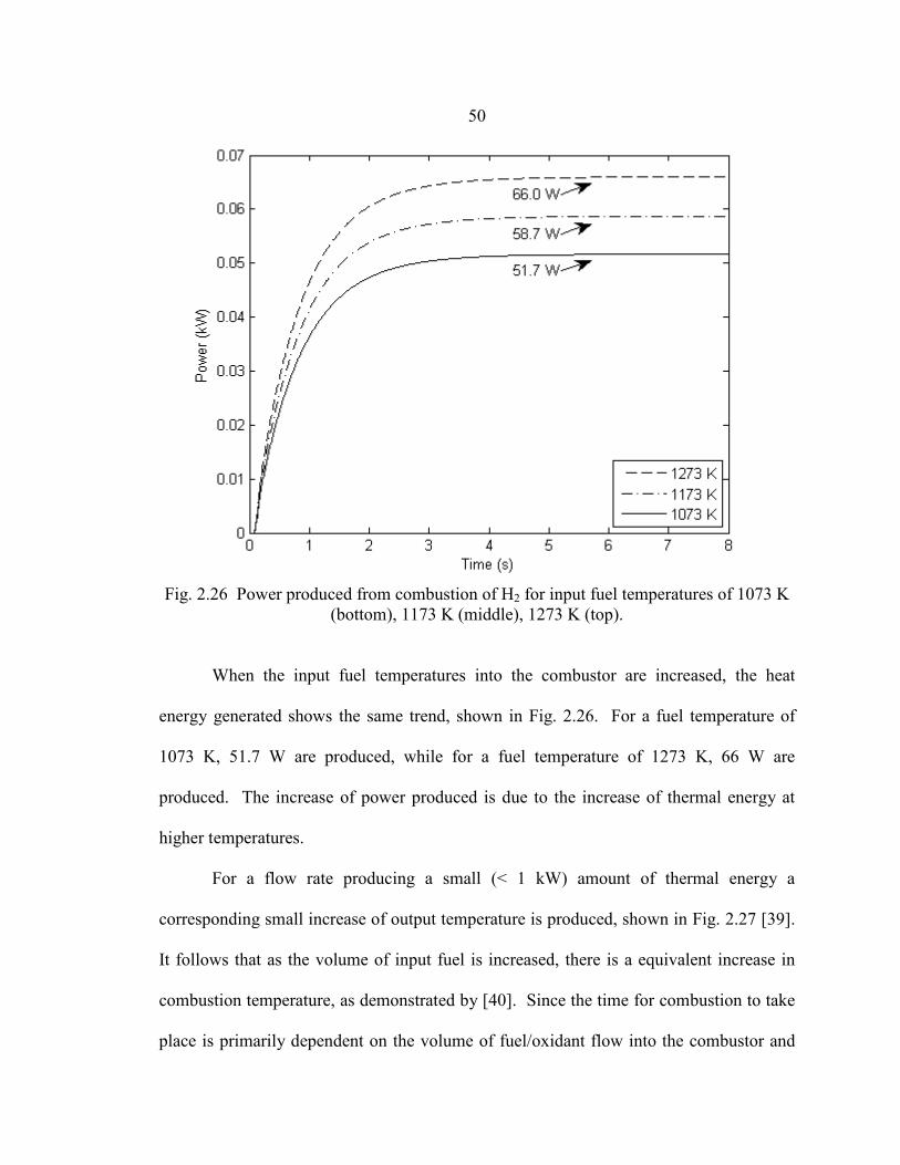
50

Fig. 2.26 Power produced from combustion of H2 for input fuel temperatures of 1073 K

(bottom), 1173 K (middle), 1273 K (top). When the input fuel temperatures into the combustor are increased, the heat

energy generated shows the same trend, shown in Fig. 2.26. For a fuel temperature of

1073 K, 51.7 W are produced, while for a fuel temperature of 1273 K, 66 W are

produced. The increase of power produced is due to the increase of thermal energy at

higher temperatures.

For a flow rate producing a small (< 1 kW) amount of thermal energy a

corresponding small increase of output temperature is produced, shown in Fig. 2.27 [39].

It follows that as the volume of input fuel is increased, there is a equivalent increase in

combustion temperature, as demonstrated by [40]. Since the time for combustion to take

place is primarily dependent on the volume of fuel/oxidant flow into the combustor and

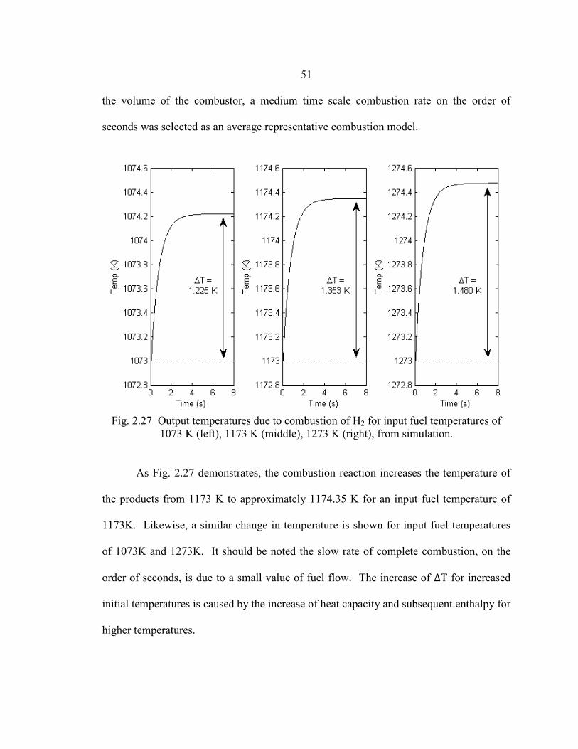
51

the volume of the combustor, a medium time scale combustion rate on the order of

seconds was selected as an average representative combustion model.

Fig. 2.27 Output temperatures due to combustion of H2 for input fuel temperatures of

1073 K (left), 1173 K (middle), 1273 K (right), from simulation. As Fig. 2.27 demonstrates, the combustion reaction increases the temperature of

the products from 1173 K to approximately 1174.35 K for an input fuel temperature of

1173K. Likewise, a similar change in temperature is shown for input fuel temperatures

of 1073K and 1273K. It should be noted the slow rate of complete combustion, on the

order of seconds, is due to a small value of fuel flow. The increase of ∆T for increased

initial temperatures is caused by the increase of heat capacity and subsequent enthalpy for

higher temperatures.

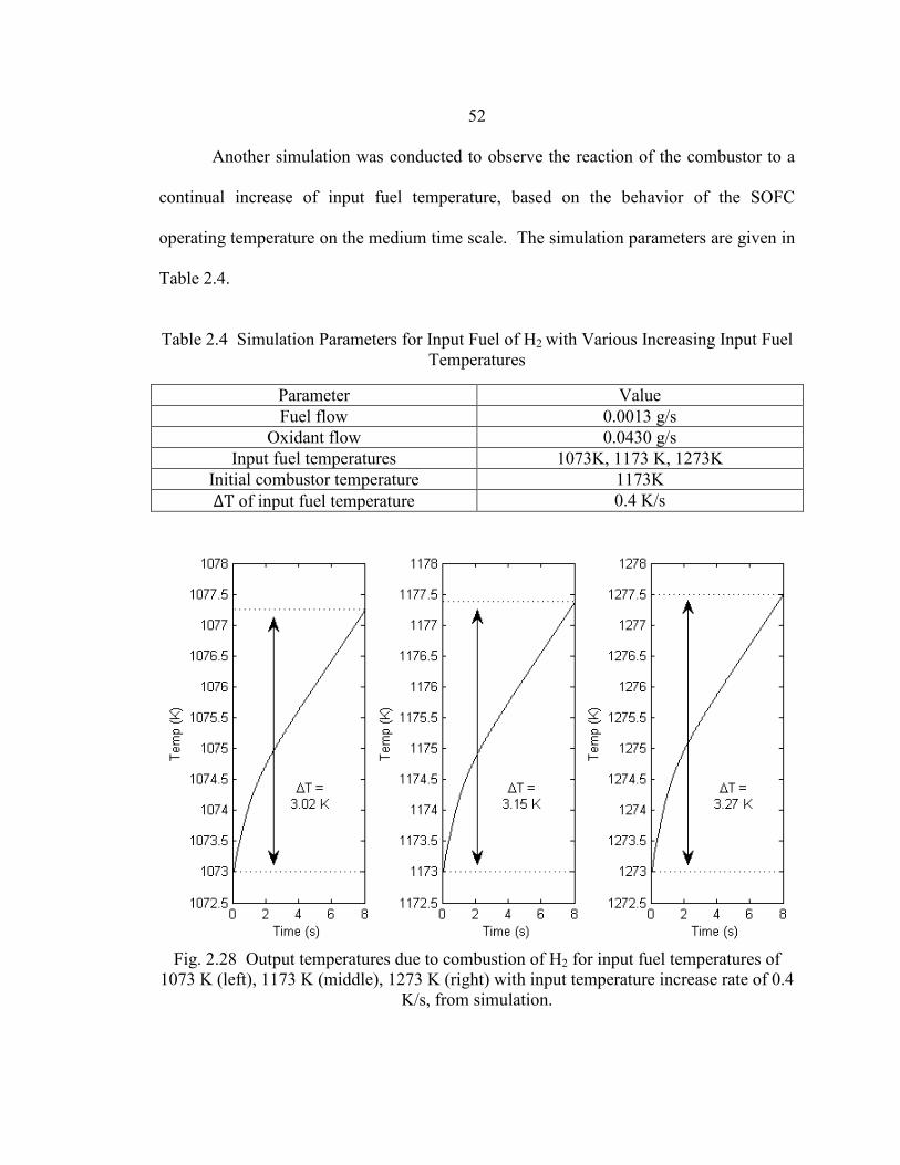
52

Another simulation was conducted to observe the reaction of the combustor to a

continual increase of input fuel temperature, based on the behavior of the SOFC

operating temperature on the medium time scale. The simulation parameters are given in

Table 2.4.

Table 2.4 Simulation Parameters for Input Fuel of H2 with Various Increasing Input Fuel

Temperatures

Parameter Value Fuel flow 0.0013 g/s

Oxidant flow 0.0430 g/s Input fuel temperatures 1073K, 1173 K, 1273K

Initial combustor temperature 1173K ∆T of input fuel temperature 0.4 K/s

Fig. 2.28 Output temperatures due to combustion of H2 for input fuel temperatures of

1073 K (left), 1173 K (middle), 1273 K (right) with input temperature increase rate of 0.4 K/s, from simulation.

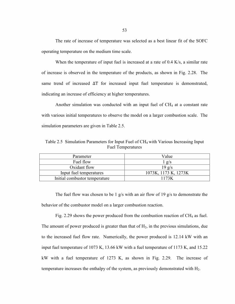
53

The rate of increase of temperature was selected as a best linear fit of the SOFC

operating temperature on the medium time scale.

When the temperature of input fuel is increased at a rate of 0.4 K/s, a similar rate

of increase is observed in the temperature of the products, as shown in Fig. 2.28. The

same trend of increased ∆T for increased input fuel temperature is demonstrated,

indicating an increase of efficiency at higher temperatures.

Another simulation was conducted with an input fuel of CH4 at a constant rate

with various initial temperatures to observe the model on a larger combustion scale. The

simulation parameters are given in Table 2.5.

Table 2.5 Simulation Parameters for Input Fuel of CH4 with Various Increasing Input

Fuel Temperatures

Parameter Value Fuel flow 1 g/s

Oxidant flow 19 g/s Input fuel temperatures 1073K, 1173 K, 1273K

Initial combustor temperature 1173K The fuel flow was chosen to be 1 g/s with an air flow of 19 g/s to demonstrate the

behavior of the combustor model on a larger combustion reaction.

Fig. 2.29 shows the power produced from the combustion reaction of CH4 as fuel.

The amount of power produced is greater than that of H2, in the previous simulations, due

to the increased fuel flow rate. Numerically, the power produced is 12.14 kW with an

input fuel temperature of 1073 K, 13.66 kW with a fuel temperature of 1173 K, and 15.22

kW with a fuel temperature of 1273 K, as shown in Fig. 2.29. The increase of

temperature increases the enthalpy of the system, as previously demonstrated with H2.

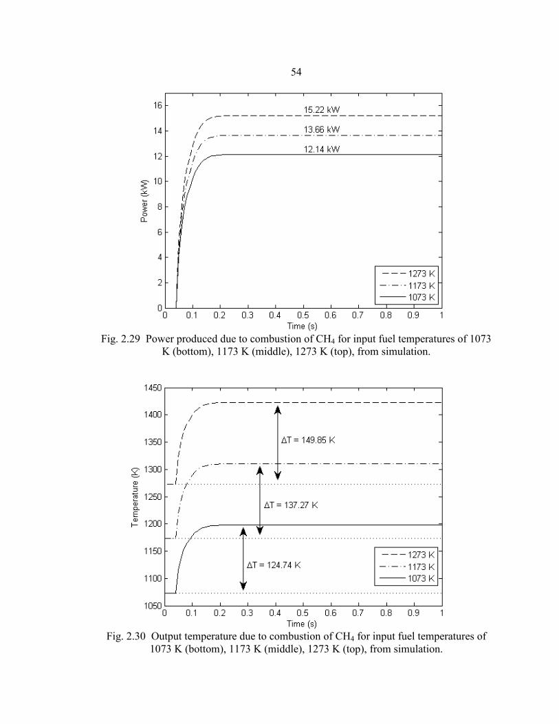
54

Fig. 2.29 Power produced due to combustion of CH4 for input fuel temperatures of 1073

K (bottom), 1173 K (middle), 1273 K (top), from simulation.

Fig. 2.30 Output temperature due to combustion of CH4 for input fuel temperatures of

1073 K (bottom), 1173 K (middle), 1273 K (top), from simulation.

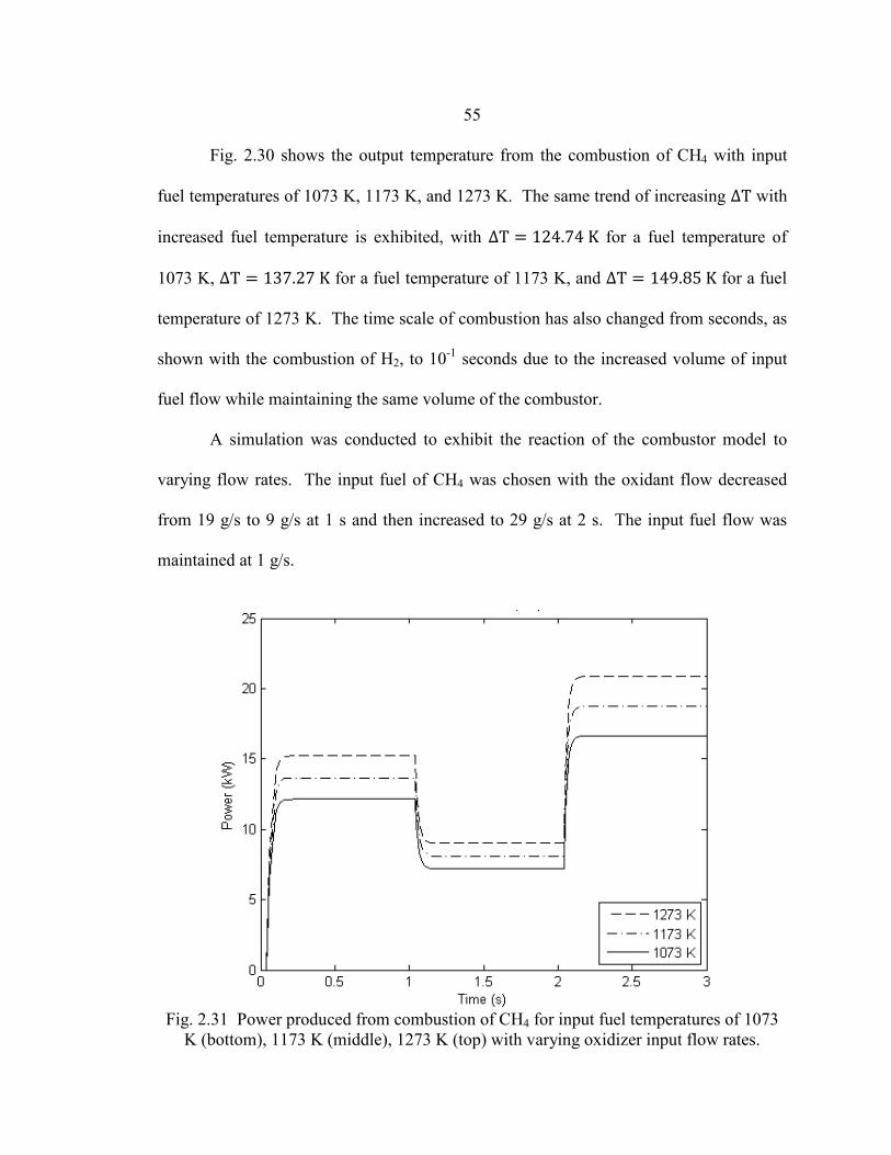
55

Fig. 2.30 shows the output temperature from the combustion of CH4 with input

fuel temperatures of 1073 K, 1173 K, and 1273 K. The same trend of increasing ∆T with

increased fuel temperature is exhibited, with ∆T = 124.74 K for a fuel temperature of

1073 K, ∆T = 137.27 K for a fuel temperature of 1173 K, and ∆T = 149.85 K for a fuel

temperature of 1273 K. The time scale of combustion has also changed from seconds, as

shown with the combustion of H2, to 10-1 seconds due to the increased volume of input

fuel flow while maintaining the same volume of the combustor.

A simulation was conducted to exhibit the reaction of the combustor model to

varying flow rates. The input fuel of CH4 was chosen with the oxidant flow decreased

from 19 g/s to 9 g/s at 1 s and then increased to 29 g/s at 2 s. The input fuel flow was

maintained at 1 g/s.

Fig. 2.31 Power produced from combustion of CH4 for input fuel temperatures of 1073

K (bottom), 1173 K (middle), 1273 K (top) with varying oxidizer input flow rates.

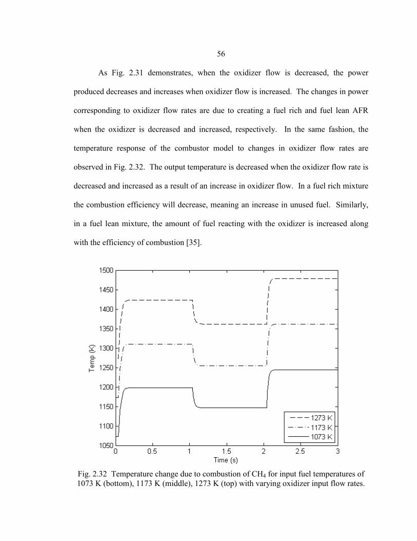
56

As Fig. 2.31 demonstrates, when the oxidizer flow is decreased, the power

produced decreases and increases when oxidizer flow is increased. The changes in power

corresponding to oxidizer flow rates are due to creating a fuel rich and fuel lean AFR

when the oxidizer is decreased and increased, respectively. In the same fashion, the

temperature response of the combustor model to changes in oxidizer flow rates are

observed in Fig. 2.32. The output temperature is decreased when the oxidizer flow rate is

decreased and increased as a result of an increase in oxidizer flow. In a fuel rich mixture

the combustion efficiency will decrease, meaning an increase in unused fuel. Similarly,

in a fuel lean mixture, the amount of fuel reacting with the oxidizer is increased along

with the efficiency of combustion [35].

Fig. 2.32 Temperature change due to combustion of CH4 for input fuel temperatures of 1073 K (bottom), 1173 K (middle), 1273 K (top) with varying oxidizer input flow rates.

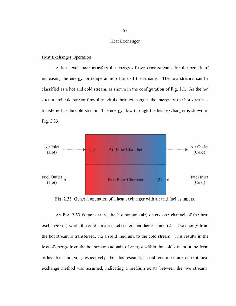
57

Heat Exchanger

Heat Exchanger Operation

A heat exchanger transfers the energy of two cross-streams for the benefit of

increasing the energy, or temperature, of one of the streams. The two streams can be

classified as a hot and cold stream, as shown in the configuration of Fig. 1.1. As the hot

stream and cold stream flow through the heat exchanger, the energy of the hot stream is

transferred to the cold stream. The energy flow through the heat exchanger is shown in

Fig. 2.33.

Fig. 2.33 General operation of a heat exchanger with air and fuel as inputs.

As Fig. 2.33 demonstrates, the hot stream (air) enters one channel of the heat

exchanger (1) while the cold stream (fuel) enters another channel (2). The energy from

the hot stream is transferred, via a solid medium, to the cold stream. This results in the

loss of energy from the hot stream and gain of energy within the cold stream in the form

of heat loss and gain, respectively. For this research, an indirect, or countercurrent, heat

exchange method was assumed, indicating a medium exists between the two streams.

58

When mixture, or direct contact, occurs between the two streams, the heat exchanger is

said to have a direct method of transferring heat. For this system, the two streams consist

of fuel and air in gaseous form.

Heat Exchanger Model of the SOFC-MT CC System

The thermodynamic mathematical model of the heat exchanger consists of a fuel

stream and an exhaust/air stream, as shown in Fig. 2.31. The fuel stream consists of the

unused fuel from the anode channel of the SOFC, and the exhaust stream consists of half

the exhaust stream from the compressor of the MT. The gas heat capacity, Cp, of the fuel

stream is calculated by (2.55). The heat capacity of the fuel stream is calculated for each

element of the fuel and multiplied by the temperature and flow rate of that particular

element to calculate the molar enthalpy of the stream, using (2.54).

Due to the operational temperatures of the SOFC and MT at approximately 1200

K and 750 K, respectively; the unused fuel from the SOFC anode channel is considered

to be the hot stream, while the exhaust from the MT is considered to be the cold stream.

The temperatures of the air and fuel outlets are the only concern for the purpose of this

research. The temperatures of the air and fuel outlets are assumed to be the temperatures

of the metal at the outlets, and are given by (2.57) and (2.58), respectively.

𝑑𝑇𝑐𝑜𝑙𝑑𝑜𝑢𝑡

𝑑𝑡=

1𝑚𝑚𝑒𝑡𝑎𝑙𝐶𝑝𝑚𝑒𝑡𝑎𝑙

��̇�𝑐𝑜𝑙𝑑𝐶𝑝𝑐𝑜𝑙𝑑�𝑇𝑐𝑜𝑙𝑑𝑖𝑛 − 𝑇𝑐𝑜𝑙𝑑𝑜𝑢𝑡� + 𝑞� (2.57)

𝑑𝑇ℎ𝑜𝑡𝑜𝑢𝑡

𝑑𝑡=

1𝑚𝑚𝑒𝑡𝑎𝑙𝐶𝑝𝑚𝑒𝑡𝑎𝑙

��̇�ℎ𝑜𝑡𝐶𝑝ℎ𝑜𝑡�𝑇ℎ𝑜𝑡𝑖𝑛 − 𝑇ℎ𝑜𝑡𝑜𝑢𝑡� − 𝑞� (2.58)

Where 𝑇𝑖𝑜𝑢𝑡 is the temperature of the metal at the i outlet, 𝑇𝑖𝑖𝑛 is the temperature

of the metal at the i inlet, 𝑚𝑚𝑒𝑡𝑎𝑙 is the mass of the heat exchanger plate, 𝐶𝑝𝑖 is the

59

specific heat capacity of the i material or stream, �̇�𝑖 is the mass flow rate of the i stream,

and 𝑞 is the rate of heat transfer found by Eq. (2.59) [42].

𝑞 =𝑒χ

𝑒𝜒

�̇�ℎ𝑜𝑡𝐶𝑝ℎ𝑜𝑡− 1

�̇�𝑐𝑜𝑙𝑑𝐶𝑝𝑐𝑜𝑙𝑑

�𝑇ℎ𝑜𝑡𝑖𝑛 − 𝑇𝑐𝑜𝑙𝑑𝑖𝑛� (2.59)

Where 𝜒 is a dimensionless parameter defined as

𝜒 = 𝑘𝑐𝑜𝑛𝑑 ∙ 𝑙𝐻𝑋 ∙ �1

�̇�ℎ𝑜𝑡𝐶𝑝ℎ𝑜𝑡

− 1

�̇�𝑐𝑜𝑙𝑑𝐶𝑝𝑐𝑜𝑙𝑑

� (2.60)

Where 𝑘𝑐𝑜𝑛𝑑 is the thermal conductivity of the streams (W/m K) and 𝑙𝐻𝑋 is the

thickness of the heat exchanger plate (mm).

The high operating temperature of the system led to the assumption that the metal

used in the heat exchanger requires a relatively large specific heat capacity. A metal of

carbon steel was selected to represent a common heat exchanger material for the

specified temperature range of the system, with a specific heat capacity of approximately

0.7 J/g K [43]. The specific heat capacity of the metal only affects the rate of heat

transfer and not the final temperatures of the streams. The steady state temperatures of

the streams will be reached on a large time scale (102-103 s) as a result of increasing the

specific heat capacity of the metal.

The inputs for the heat exchanger block are: mass flow rate of unused fuel from

the anode channel of the SOFC (mol/s) and associated temperature of stream (K), along

with half of the mass flow rate of exhaust from the compressor of the MT (mol/s) and

associated temperature of the stream (K). The outputs of the block are the temperatures

of the fuel and air streams at the outlets of the heat exchanger (K).

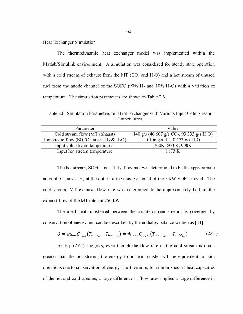
60

Heat Exchanger Simulation

The thermodynamic heat exchanger model was implemented within the

Matlab/Simulink environment. A simulation was considered for steady state operation

with a cold stream of exhaust from the MT (CO2 and H2O) and a hot stream of unused

fuel from the anode channel of the SOFC (90% H2 and 10% H2O) with a variation of

temperature. The simulation parameters are shown in Table 2.6.

Table 2.6 Simulation Parameters for Heat Exchanger with Various Input Cold Stream

Temperatures

Parameter Value Cold stream flow (MT exhaust) 140 g/s (46.667 g/s CO2, 93.333 g/s H2O)

Hot stream flow (SOFC unused H2 & H2O) 0.106 g/s H2, 0.773 g/s H2O Input cold stream temperatures 700K, 800 K, 900K Input hot stream temperature 1173 K

The hot stream, SOFC unused H2, flow rate was determined to be the approximate

amount of unused H2 at the outlet of the anode channel of the 5 kW SOFC model. The

cold stream, MT exhaust, flow rate was determined to be approximately half of the

exhaust flow of the MT rated at 250 kW.

The ideal heat transferred between the countercurrent streams is governed by

conservation of energy and can be described by the enthalpy balance written as [41]

𝑄 = �̇�ℎ𝑜𝑡𝐶𝑝ℎ𝑜𝑡�𝑇ℎ𝑜𝑡𝑖𝑛 − 𝑇ℎ𝑜𝑡𝑜𝑢𝑡� = �̇�𝑐𝑜𝑙𝑑𝐶𝑝𝑐𝑜𝑙𝑑�𝑇𝑐𝑜𝑙𝑑𝑜𝑢𝑡 − 𝑇𝑐𝑜𝑙𝑑𝑖𝑛� (2.61) As Eq. (2.61) suggests, even though the flow rate of the cold stream is much

greater than the hot stream, the energy from heat transfer will be equivalent in both

directions due to conservation of energy. Furthermore, for similar specific heat capacities

of the hot and cold streams, a large difference in flow rates implies a large difference in

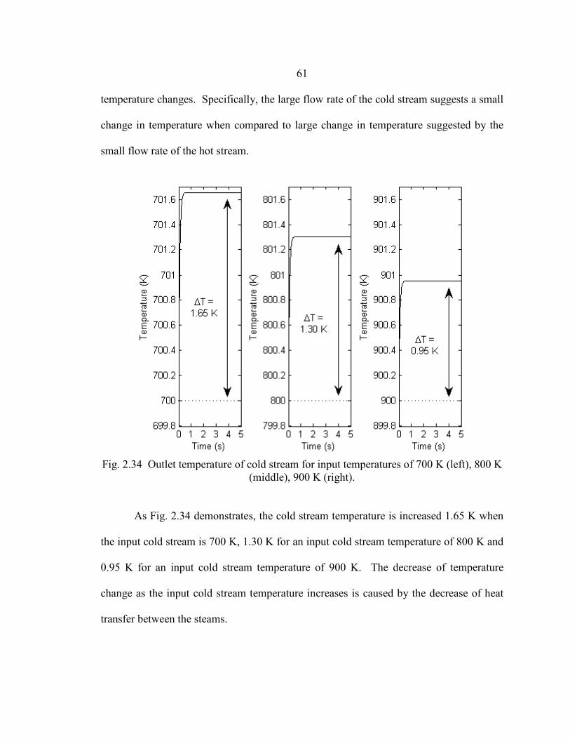
61

temperature changes. Specifically, the large flow rate of the cold stream suggests a small

change in temperature when compared to large change in temperature suggested by the

small flow rate of the hot stream.

Fig. 2.34 Outlet temperature of cold stream for input temperatures of 700 K (left), 800 K

(middle), 900 K (right). As Fig. 2.34 demonstrates, the cold stream temperature is increased 1.65 K when

the input cold stream is 700 K, 1.30 K for an input cold stream temperature of 800 K and

0.95 K for an input cold stream temperature of 900 K. The decrease of temperature

change as the input cold stream temperature increases is caused by the decrease of heat

transfer between the steams.

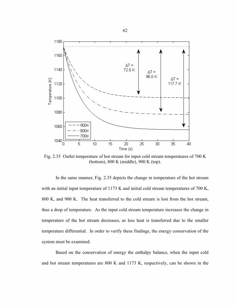
62

Fig. 2.35 Outlet temperature of hot stream for input cold stream temperatures of 700 K

(bottom), 800 K (middle), 900 K (top). In the same manner, Fig. 2.35 depicts the change in temperature of the hot stream

with an initial input temperature of 1173 K and initial cold stream temperatures of 700 K,

800 K, and 900 K. The heat transferred to the cold stream is lost from the hot stream,

thus a drop of temperature. As the input cold stream temperature increases the change in

temperature of the hot stream decreases, as less heat is transferred due to the smaller

temperature differential. In order to verify these findings, the energy conservation of the

system must be examined.

Based on the conservation of energy the enthalpy balance, when the input cold

and hot stream temperatures are 800 K and 1173 K, respectively, can be shown in the

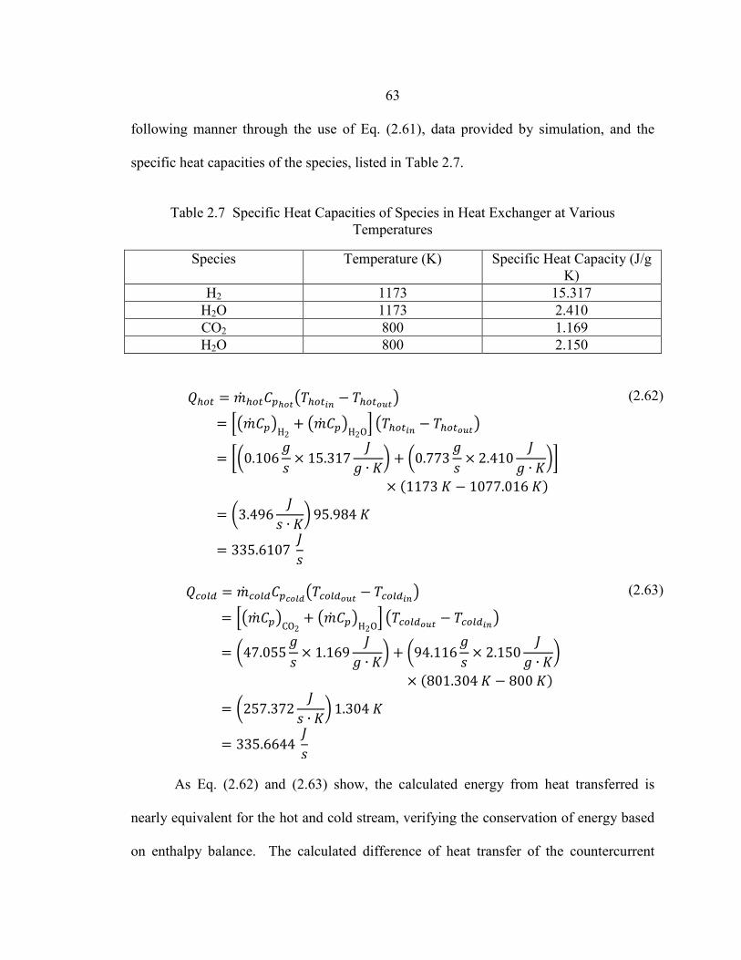
63

following manner through the use of Eq. (2.61), data provided by simulation, and the

specific heat capacities of the species, listed in Table 2.7.

Table 2.7 Specific Heat Capacities of Species in Heat Exchanger at Various

Temperatures

Species Temperature (K) Specific Heat Capacity (J/g K)

H2 1173 15.317 H2O 1173 2.410 CO2 800 1.169 H2O 800 2.150

𝑄ℎ𝑜𝑡 = �̇�ℎ𝑜𝑡𝐶𝑝ℎ𝑜𝑡�𝑇ℎ𝑜𝑡𝑖𝑛 − 𝑇ℎ𝑜𝑡𝑜𝑢𝑡�

= ���̇�𝐶𝑝�H2

+ ��̇�𝐶𝑝�H2O

� �𝑇ℎ𝑜𝑡𝑖𝑛 − 𝑇ℎ𝑜𝑡𝑜𝑢𝑡�

= ��0.106𝑔𝑠

× 15.317𝐽

𝑔 ∙ 𝐾� + �0.773

𝑔𝑠

× 2.410𝐽

𝑔 ∙ 𝐾��

× (1173 𝐾 − 1077.016 𝐾)

= �3.496𝐽

𝑠 ∙ 𝐾� 95.984 𝐾

= 335.6107 𝐽𝑠

(2.62)

𝑄𝑐𝑜𝑙𝑑 = �̇�𝑐𝑜𝑙𝑑𝐶𝑝𝑐𝑜𝑙𝑑�𝑇𝑐𝑜𝑙𝑑𝑜𝑢𝑡 − 𝑇𝑐𝑜𝑙𝑑𝑖𝑛�

= ���̇�𝐶𝑝�CO2

+ ��̇�𝐶𝑝�H2O

� �𝑇𝑐𝑜𝑙𝑑𝑜𝑢𝑡 − 𝑇𝑐𝑜𝑙𝑑𝑖𝑛�

= �47.055𝑔𝑠

× 1.169𝐽

𝑔 ∙ 𝐾� + �94.116

𝑔𝑠

× 2.150𝐽

𝑔 ∙ 𝐾�

× (801.304 𝐾 − 800 𝐾)

= �257.372𝐽

𝑠 ∙ 𝐾� 1.304 𝐾

= 335.6644 𝐽𝑠

(2.63)

As Eq. (2.62) and (2.63) show, the calculated energy from heat transferred is

nearly equivalent for the hot and cold stream, verifying the conservation of energy based

on enthalpy balance. The calculated difference of heat transfer of the countercurrent

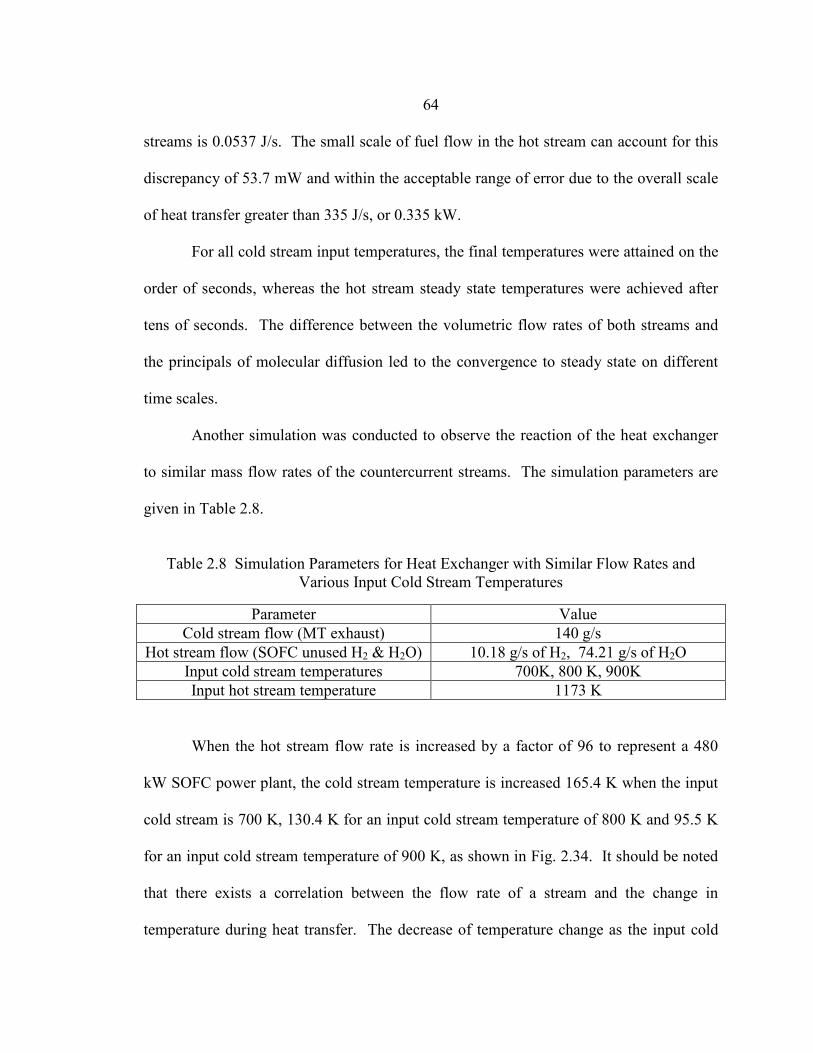
64

streams is 0.0537 J/s. The small scale of fuel flow in the hot stream can account for this

discrepancy of 53.7 mW and within the acceptable range of error due to the overall scale

of heat transfer greater than 335 J/s, or 0.335 kW.

For all cold stream input temperatures, the final temperatures were attained on the

order of seconds, whereas the hot stream steady state temperatures were achieved after

tens of seconds. The difference between the volumetric flow rates of both streams and

the principals of molecular diffusion led to the convergence to steady state on different

time scales.

Another simulation was conducted to observe the reaction of the heat exchanger

to similar mass flow rates of the countercurrent streams. The simulation parameters are

given in Table 2.8.

Table 2.8 Simulation Parameters for Heat Exchanger with Similar Flow Rates and

Various Input Cold Stream Temperatures

Parameter Value Cold stream flow (MT exhaust) 140 g/s

Hot stream flow (SOFC unused H2 & H2O) 10.18 g/s of H2, 74.21 g/s of H2O Input cold stream temperatures 700K, 800 K, 900K Input hot stream temperature 1173 K

When the hot stream flow rate is increased by a factor of 96 to represent a 480

kW SOFC power plant, the cold stream temperature is increased 165.4 K when the input

cold stream is 700 K, 130.4 K for an input cold stream temperature of 800 K and 95.5 K

for an input cold stream temperature of 900 K, as shown in Fig. 2.34. It should be noted

that there exists a correlation between the flow rate of a stream and the change in

temperature during heat transfer. The decrease of temperature change as the input cold

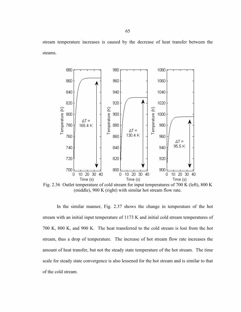
65

stream temperature increases is caused by the decrease of heat transfer between the

steams.

Fig. 2.36 Outlet temperature of cold stream for input temperatures of 700 K (left), 800 K

(middle), 900 K (right) with similar hot stream flow rate. In the similar manner, Fig. 2.37 shows the change in temperature of the hot

stream with an initial input temperature of 1173 K and initial cold stream temperatures of

700 K, 800 K, and 900 K. The heat transferred to the cold stream is lost from the hot

stream, thus a drop of temperature. The increase of hot stream flow rate increases the

amount of heat transfer, but not the steady state temperature of the hot stream. The time

scale for steady state convergence is also lessened for the hot stream and is similar to that

of the cold stream.

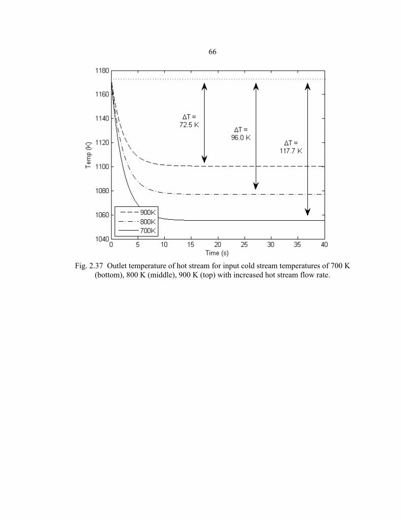
66

Fig. 2.37 Outlet temperature of hot stream for input cold stream temperatures of 700 K

(bottom), 800 K (middle), 900 K (top) with increased hot stream flow rate.

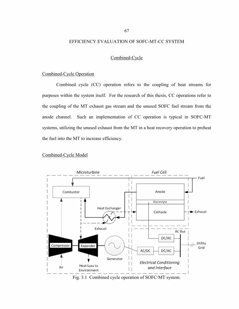
67

EFFICIENCY EVALUATION OF SOFC-MT-CC SYSTEM

Combined-Cycle

Combined-Cycle Operation

Combined cycle (CC) operation refers to the coupling of heat streams for

purposes within the system itself. For the research of this thesis, CC operations refer to

the coupling of the MT exhaust gas stream and the unused SOFC fuel stream from the

anode channel. Such an implementation of CC operation is typical in SOFC-MT

systems, utilizing the unused exhaust from the MT in a heat recovery operation to preheat

the fuel into the MT to increase efficiency.

Combined-Cycle Model

Fig. 3.1 Combined cycle operation of SOFC/MT system.

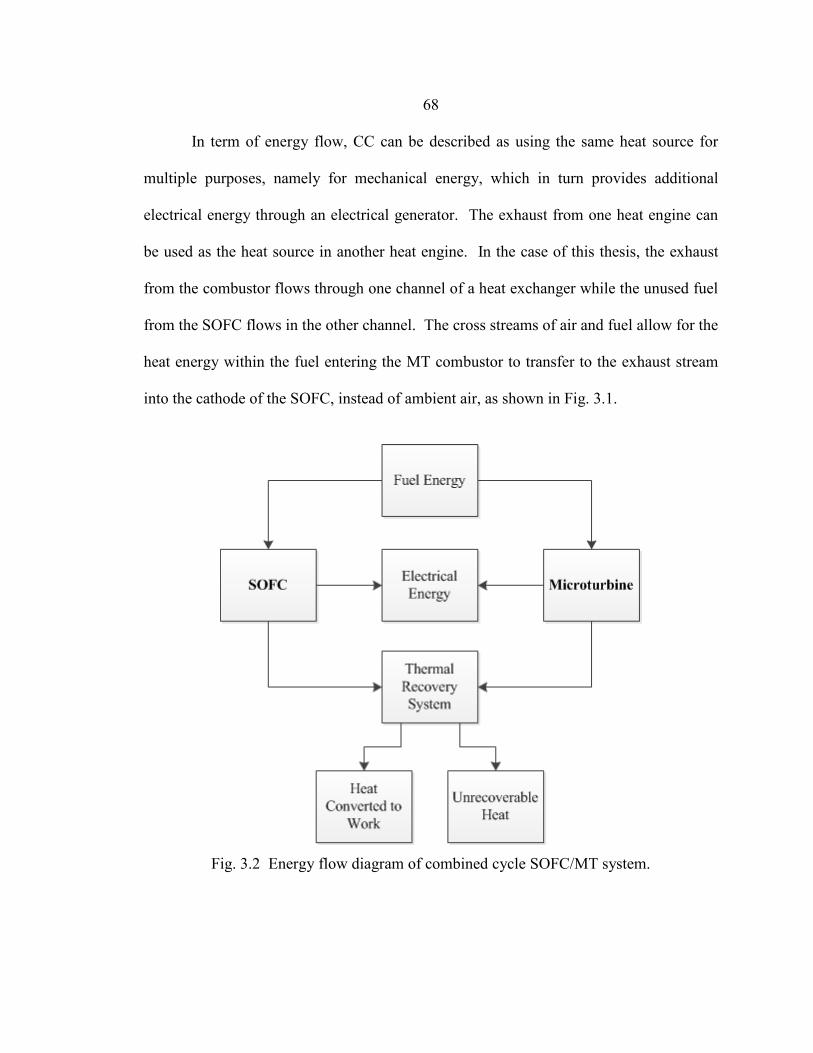
68

In term of energy flow, CC can be described as using the same heat source for

multiple purposes, namely for mechanical energy, which in turn provides additional

electrical energy through an electrical generator. The exhaust from one heat engine can

be used as the heat source in another heat engine. In the case of this thesis, the exhaust

from the combustor flows through one channel of a heat exchanger while the unused fuel

from the SOFC flows in the other channel. The cross streams of air and fuel allow for the

heat energy within the fuel entering the MT combustor to transfer to the exhaust stream

into the cathode of the SOFC, instead of ambient air, as shown in Fig. 3.1.

Fig. 3.2 Energy flow diagram of combined cycle SOFC/MT system.

69

The energy flow of the system begins with the fuel energy provided to the SOFC

and MT, which, in turn produce electrical energy. The heat losses of each device are

utilized with a thermal recovery system in the form of a combined cycle. The thermal

recovery system either converts the heat to work or is lost to the environment. The

energy flow of the system is visualized in Fig. 3.2.

By coupling the exhaust stream of the MT to the combustor and heat exchanger,

along with the unused fuel from the SOFC anode channel to the heat exchanger, the

system is said to be in CC operations. For the system to not operate in CC the heat

exchanger would be disconnected, causing the unused fuel from the SOFC anode channel

to not be preheated and utilized within the MT combustor and the exhaust stream from

the MT to succumb to heat loss to the environment; ultimately decreasing the overall

efficiency of the system through more losses.

Combined-Cycle Simulation

Table 3.1 Simulation Parameters of SOFC-MT-CC Model

Parameter Value Fuel cell

SOFC power plant 220 V/480 kW Twelve 40 kW SOFC arrays connected in parallel

SOFC array 220 V/40 kW, consisting of 4 (series) x 2(parallel) = eight 5 kW SOFC stacks

Fuel molar flow rate 9.216 mol/s (90% H2 + 10% H2O) Air molar flow rate 110.592 mol/s Pressures (anode & cathode) 3 atm Initial fuel & air temperature 1173 K

Microturbine Rated power 250 kW Operation efficiency 35 % Operation temperature 750 K

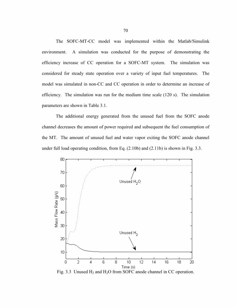
70

The SOFC-MT-CC model was implemented within the Matlab/Simulink

environment. A simulation was conducted for the purpose of demonstrating the

efficiency increase of CC operation for a SOFC-MT system. The simulation was

considered for steady state operation over a variety of input fuel temperatures. The

model was simulated in non-CC and CC operation in order to determine an increase of

efficiency. The simulation was run for the medium time scale (120 s). The simulation

parameters are shown in Table 3.1.

The additional energy generated from the unused fuel from the SOFC anode

channel decreases the amount of power required and subsequent the fuel consumption of

the MT. The amount of unused fuel and water vapor exiting the SOFC anode channel

under full load operating condition, from Eq. (2.10b) and (2.11b) is shown in Fig. 3.3.

Fig. 3.3 Unused H2 and H2O from SOFC anode channel in CC operation.

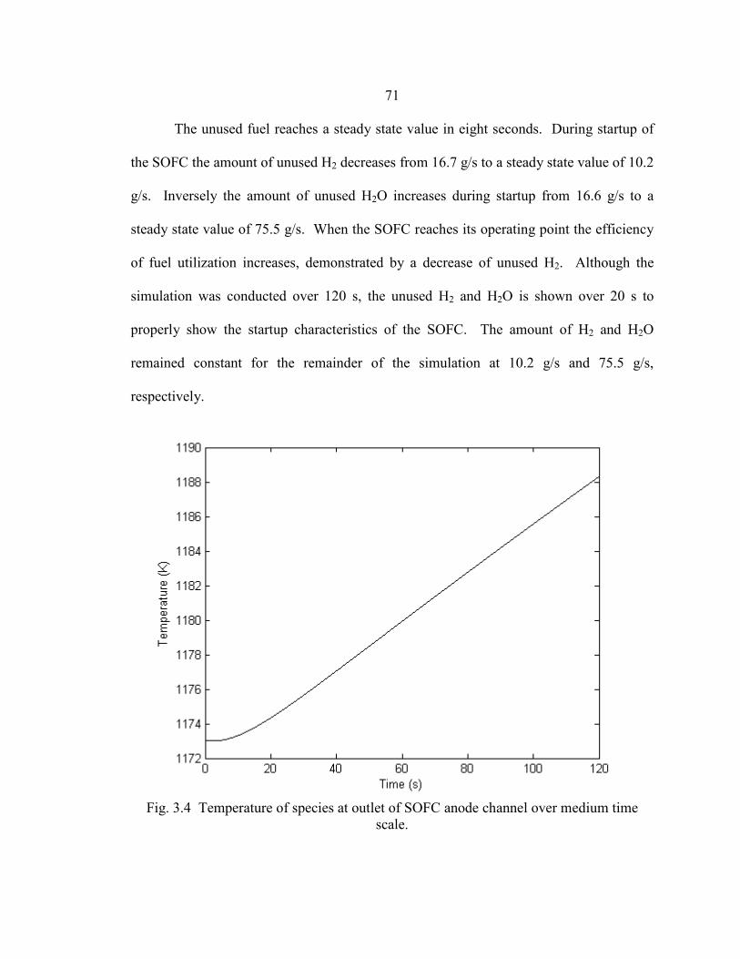
71

The unused fuel reaches a steady state value in eight seconds. During startup of

the SOFC the amount of unused H2 decreases from 16.7 g/s to a steady state value of 10.2

g/s. Inversely the amount of unused H2O increases during startup from 16.6 g/s to a

steady state value of 75.5 g/s. When the SOFC reaches its operating point the efficiency

of fuel utilization increases, demonstrated by a decrease of unused H2. Although the

simulation was conducted over 120 s, the unused H2 and H2O is shown over 20 s to

properly show the startup characteristics of the SOFC. The amount of H2 and H2O

remained constant for the remainder of the simulation at 10.2 g/s and 75.5 g/s,

respectively.

Fig. 3.4 Temperature of species at outlet of SOFC anode channel over medium time

scale.

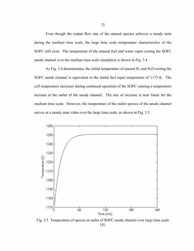
72

Even though the output flow rate of the unused species achieves a steady state

during the medium time scale, the large time scale temperature characteristics of the

SOFC still exist. The temperature of the unused fuel and water vapor exiting the SOFC

anode channel over the medium time scale simulation is shown in Fig. 3.4.

As Fig. 3.4 demonstrates, the initial temperature of unused H2 and H2O exiting the

SOFC anode channel is equivalent to the initial fuel input temperature of 1173 K. The

cell temperature increases during continued operation of the SOFC causing a temperature

increase at the outlet of the anode channel. The rate of increase is near linear for the

medium time scale. However, the temperature of the outlet species of the anode channel

arrives at a steady state value over the large time scale, as shown in Fig. 3.5.

Fig. 3.5 Temperature of species at outlet of SOFC anode channel over large time scale

[4].

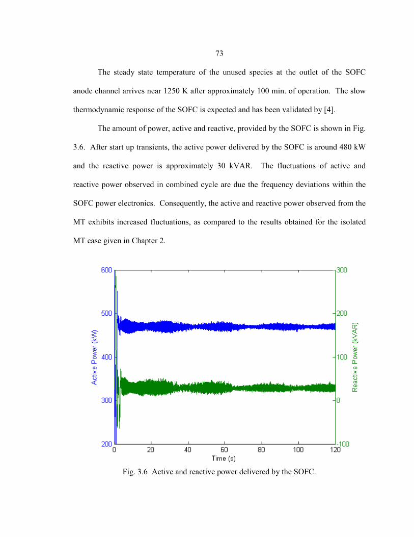
73

The steady state temperature of the unused species at the outlet of the SOFC

anode channel arrives near 1250 K after approximately 100 min. of operation. The slow

thermodynamic response of the SOFC is expected and has been validated by [4].

The amount of power, active and reactive, provided by the SOFC is shown in Fig.

3.6. After start up transients, the active power delivered by the SOFC is around 480 kW

and the reactive power is approximately 30 kVAR. The fluctuations of active and

reactive power observed in combined cycle are due the frequency deviations within the

SOFC power electronics. Consequently, the active and reactive power observed from the

MT exhibits increased fluctuations, as compared to the results obtained for the isolated

MT case given in Chapter 2.

Fig. 3.6 Active and reactive power delivered by the SOFC.

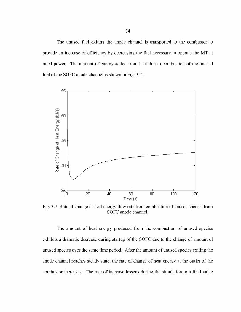
74

The unused fuel exiting the anode channel is transported to the combustor to

provide an increase of efficiency by decreasing the fuel necessary to operate the MT at

rated power. The amount of energy added from heat due to combustion of the unused

fuel of the SOFC anode channel is shown in Fig. 3.7.

Fig. 3.7 Rate of change of heat energy flow rate from combustion of unused species from

SOFC anode channel. The amount of heat energy produced from the combustion of unused species

exhibits a dramatic decrease during startup of the SOFC due to the change of amount of

unused species over the same time period. After the amount of unused species exiting the

anode channel reaches steady state, the rate of change of heat energy at the outlet of the

combustor increases. The rate of increase lessens during the simulation to a final value

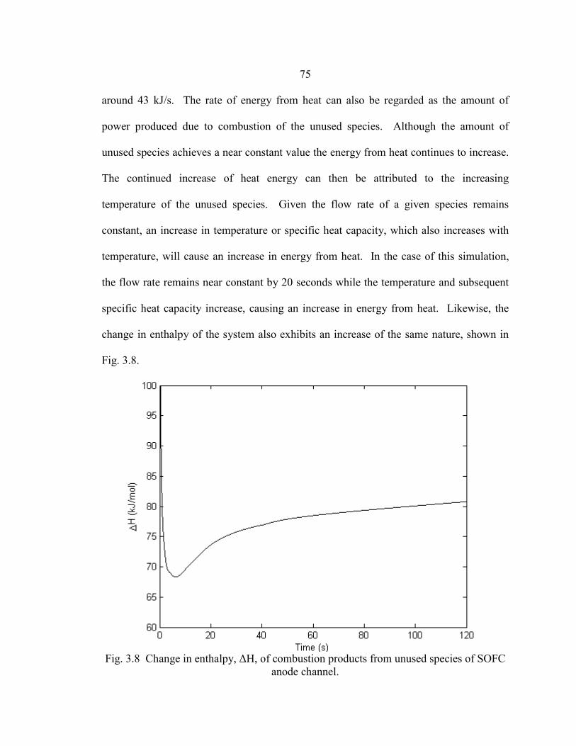
75

around 43 kJ/s. The rate of energy from heat can also be regarded as the amount of

power produced due to combustion of the unused species. Although the amount of

unused species achieves a near constant value the energy from heat continues to increase.

The continued increase of heat energy can then be attributed to the increasing

temperature of the unused species. Given the flow rate of a given species remains

constant, an increase in temperature or specific heat capacity, which also increases with

temperature, will cause an increase in energy from heat. In the case of this simulation,

the flow rate remains near constant by 20 seconds while the temperature and subsequent

specific heat capacity increase, causing an increase in energy from heat. Likewise, the

change in enthalpy of the system also exhibits an increase of the same nature, shown in

Fig. 3.8.

Fig. 3.8 Change in enthalpy, ΔH, of combustion products from unused species of SOFC

anode channel.

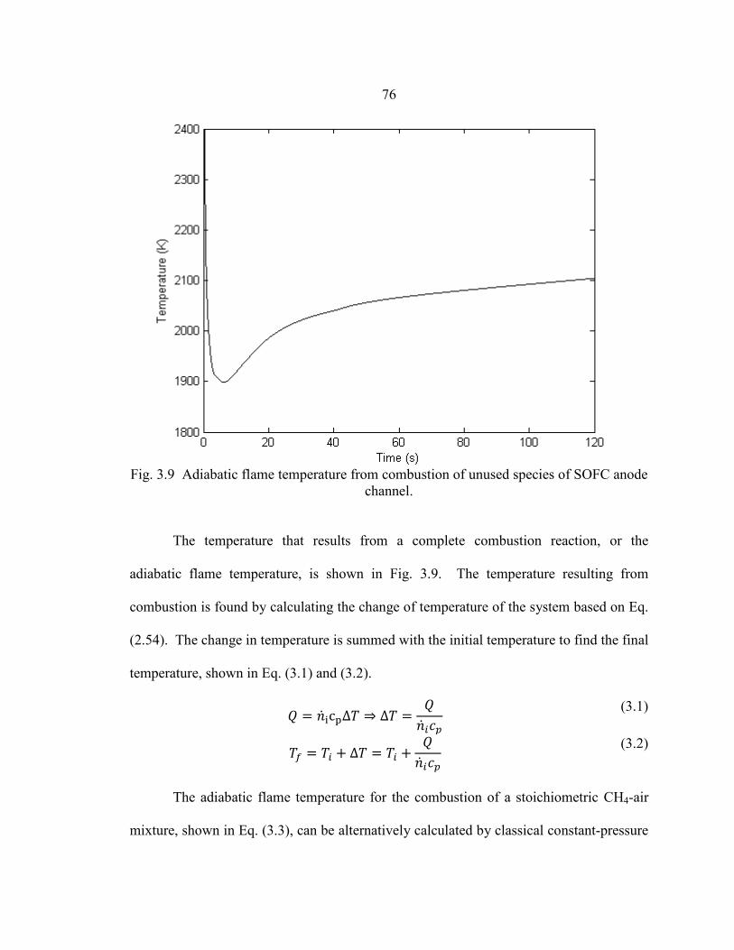
76

Fig. 3.9 Adiabatic flame temperature from combustion of unused species of SOFC anode

channel. The temperature that results from a complete combustion reaction, or the

adiabatic flame temperature, is shown in Fig. 3.9. The temperature resulting from

combustion is found by calculating the change of temperature of the system based on Eq.

(2.54). The change in temperature is summed with the initial temperature to find the final

temperature, shown in Eq. (3.1) and (3.2).

𝑄 = �̇�icpΔ𝑇 ⇒ Δ𝑇 =𝑄

�̇�𝑖𝑐𝑝

(3.1)

𝑇𝑓 = 𝑇𝑖 + Δ𝑇 = 𝑇𝑖 +𝑄

�̇�𝑖𝑐𝑝

(3.2)

The adiabatic flame temperature for the combustion of a stoichiometric CH4-air

mixture, shown in Eq. (3.3), can be alternatively calculated by classical constant-pressure

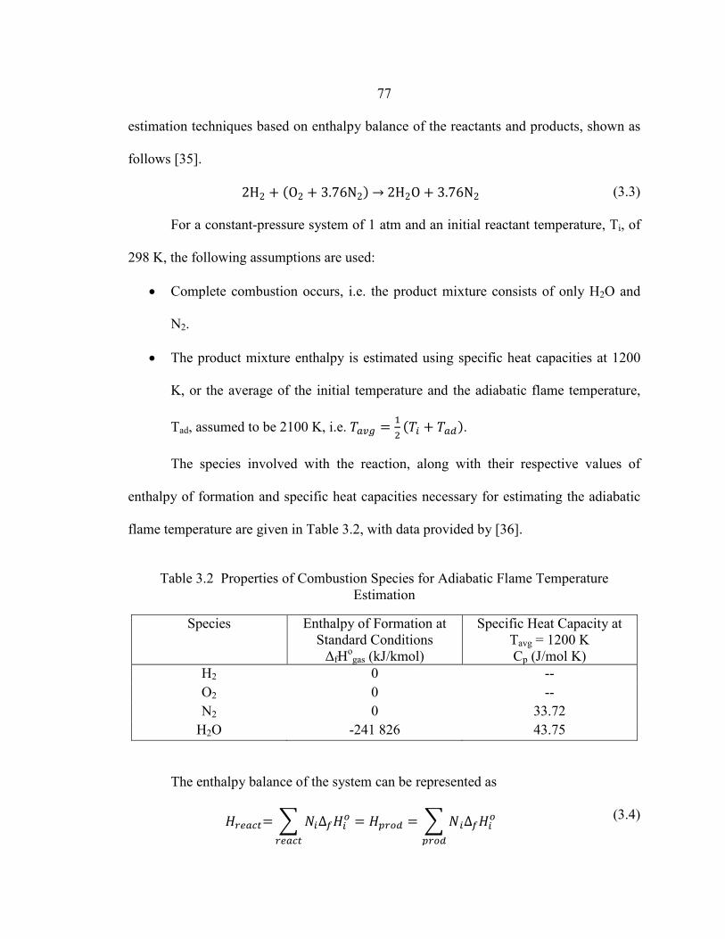
77

estimation techniques based on enthalpy balance of the reactants and products, shown as

follows [35].

2H2 + (O2 + 3.76N2) → 2H2O + 3.76N2 (3.3) For a constant-pressure system of 1 atm and an initial reactant temperature, Ti, of

298 K, the following assumptions are used:

• Complete combustion occurs, i.e. the product mixture consists of only H2O and

N2.

• The product mixture enthalpy is estimated using specific heat capacities at 1200

K, or the average of the initial temperature and the adiabatic flame temperature,

Tad, assumed to be 2100 K, i.e. 𝑇𝑎𝑣𝑔 = 12

(𝑇𝑖 + 𝑇𝑎𝑑).

The species involved with the reaction, along with their respective values of

enthalpy of formation and specific heat capacities necessary for estimating the adiabatic

flame temperature are given in Table 3.2, with data provided by [36].

Table 3.2 Properties of Combustion Species for Adiabatic Flame Temperature

Estimation

Species Enthalpy of Formation at Standard Conditions

ΔfHogas (kJ/kmol)

Specific Heat Capacity at Tavg = 1200 K Cp (J/mol K)

H2 0 -- O2 0 -- N2 0 33.72

H2O -241 826 43.75 The enthalpy balance of the system can be represented as

𝐻𝑟𝑒𝑎𝑐𝑡= � 𝑁𝑖Δ𝑓𝐻𝑖𝑜

𝑟𝑒𝑎𝑐𝑡

= 𝐻𝑝𝑟𝑜𝑑 = � 𝑁𝑖Δ𝑓𝐻𝑖𝑜

𝑝𝑟𝑜𝑑

(3.4)

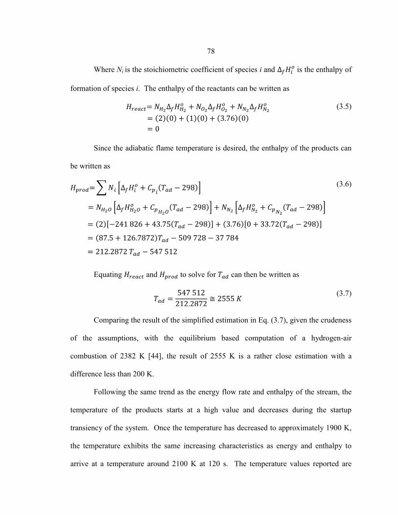
78

Where Ni is the stoichiometric coefficient of species i and Δ𝑓𝐻𝑖𝑜 is the enthalpy of

formation of species i. The enthalpy of the reactants can be written as

𝐻𝑟𝑒𝑎𝑐𝑡= 𝑁𝐻2Δ𝑓𝐻𝐻2𝑜 + 𝑁𝑂2Δ𝑓𝐻𝑂2

𝑜 + 𝑁𝑁2Δ𝑓𝐻𝑁2𝑜

= (2)(0) + (1)(0) + (3.76)(0) = 0

(3.5)

Since the adiabatic flame temperature is desired, the enthalpy of the products can

be written as

𝐻𝑝𝑟𝑜𝑑= � 𝑁𝑖 �Δ𝑓𝐻𝑖𝑜 + 𝐶𝑝𝑖

(𝑇𝑎𝑑 − 298)�

= 𝑁𝐻2𝑂 �Δ𝑓𝐻𝐻2𝑂𝑜 + 𝐶𝑝𝐻2𝑂

(𝑇𝑎𝑑 − 298)� + 𝑁𝑁2 �Δ𝑓𝐻𝑁2𝑜 + 𝐶𝑝𝑁2

(𝑇𝑎𝑑 − 298)�

= (2)[−241 826 + 43.75(𝑇𝑎𝑑 − 298)] + (3.76)[0 + 33.72(𝑇𝑎𝑑 − 298)]

= (87.5 + 126.7872)𝑇𝑎𝑑 − 509 728 − 37 784

= 212.2872 𝑇𝑎𝑑 − 547 512

(3.6)

Equating 𝐻𝑟𝑒𝑎𝑐𝑡 and 𝐻𝑝𝑟𝑜𝑑 to solve for 𝑇𝑎𝑑 can then be written as

𝑇𝑎𝑑 =547 512

212.2872≅ 2555 𝐾

(3.7)

Comparing the result of the simplified estimation in Eq. (3.7), given the crudeness

of the assumptions, with the equilibrium based computation of a hydrogen-air

combustion of 2382 K [44], the result of 2555 K is a rather close estimation with a

difference less than 200 K.

Following the same trend as the energy flow rate and enthalpy of the stream, the

temperature of the products starts at a high value and decreases during the startup

transiency of the system. Once the temperature has decreased to approximately 1900 K,

the temperature exhibits the same increasing characteristics as energy and enthalpy to

arrive at a temperature around 2100 K at 120 s. The temperature values reported are

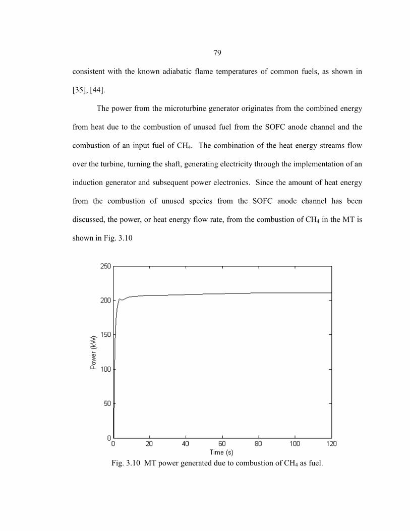
79

consistent with the known adiabatic flame temperatures of common fuels, as shown in

[35], [44].

The power from the microturbine generator originates from the combined energy

from heat due to the combustion of unused fuel from the SOFC anode channel and the

combustion of an input fuel of CH4. The combination of the heat energy streams flow

over the turbine, turning the shaft, generating electricity through the implementation of an

induction generator and subsequent power electronics. Since the amount of heat energy

from the combustion of unused species from the SOFC anode channel has been

discussed, the power, or heat energy flow rate, from the combustion of CH4 in the MT is

shown in Fig. 3.10

Fig. 3.10 MT power generated due to combustion of CH4 as fuel.

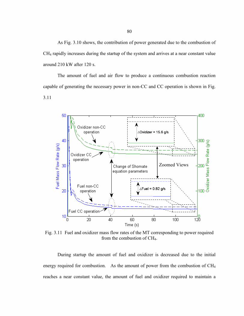
80

As Fig. 3.10 shows, the contribution of power generated due to the combustion of

CH4 rapidly increases during the startup of the system and arrives at a near constant value

around 210 kW after 120 s.

The amount of fuel and air flow to produce a continuous combustion reaction

capable of generating the necessary power in non-CC and CC operation is shown in Fig.

3.11

Fig. 3.11 Fuel and oxidizer mass flow rates of the MT corresponding to power required

from the combustion of CH4. During startup the amount of fuel and oxidizer is decreased due to the initial

energy required for combustion. As the amount of power from the combustion of CH4

reaches a near constant value, the amount of fuel and oxidizer required to maintain a

Zoomed Views

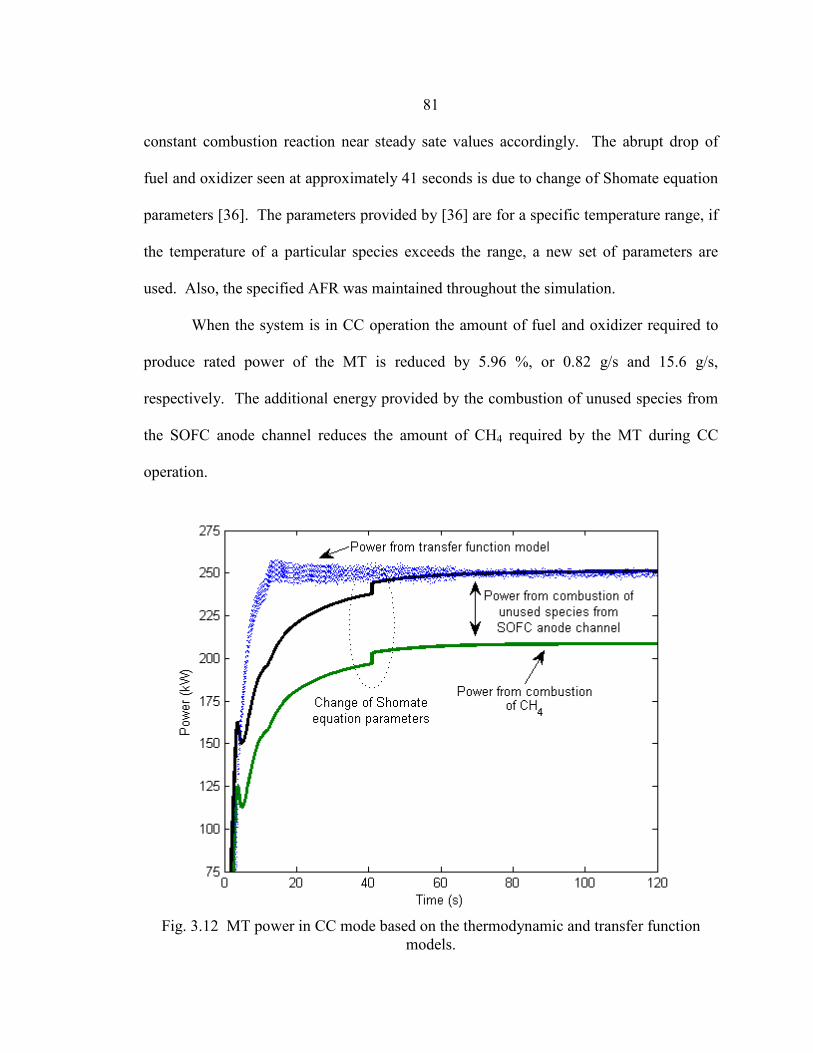
81

constant combustion reaction near steady sate values accordingly. The abrupt drop of

fuel and oxidizer seen at approximately 41 seconds is due to change of Shomate equation

parameters [36]. The parameters provided by [36] are for a specific temperature range, if

the temperature of a particular species exceeds the range, a new set of parameters are

used. Also, the specified AFR was maintained throughout the simulation.

When the system is in CC operation the amount of fuel and oxidizer required to

produce rated power of the MT is reduced by 5.96 %, or 0.82 g/s and 15.6 g/s,

respectively. The additional energy provided by the combustion of unused species from

the SOFC anode channel reduces the amount of CH4 required by the MT during CC

operation.

Fig. 3.12 MT power in CC mode based on the thermodynamic and transfer function

models.

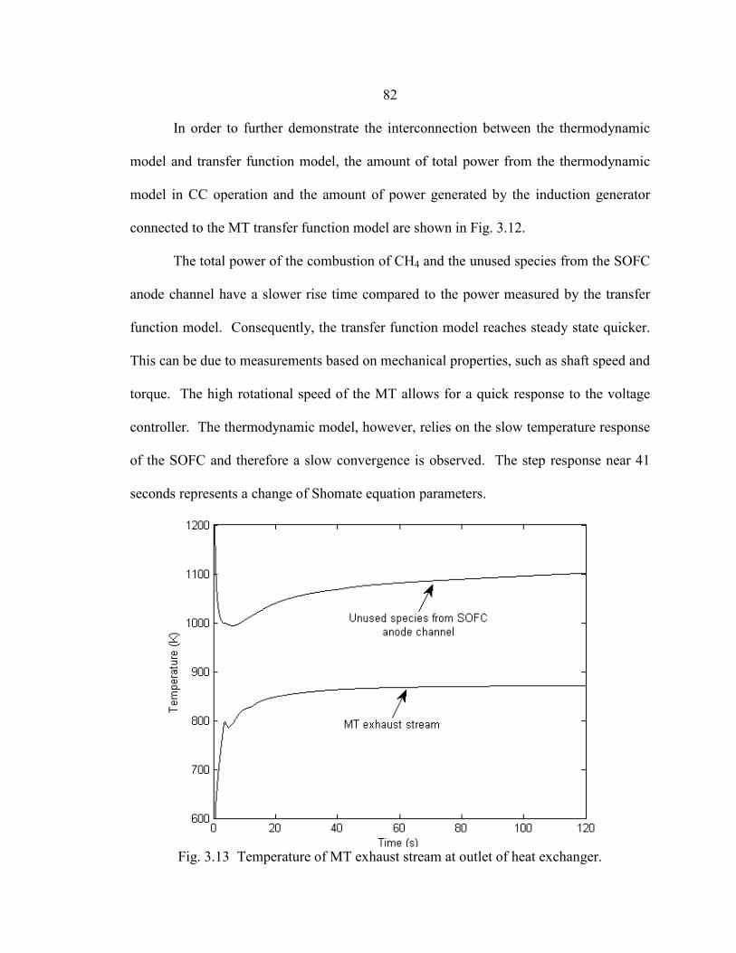
82

In order to further demonstrate the interconnection between the thermodynamic

model and transfer function model, the amount of total power from the thermodynamic

model in CC operation and the amount of power generated by the induction generator

connected to the MT transfer function model are shown in Fig. 3.12.

The total power of the combustion of CH4 and the unused species from the SOFC

anode channel have a slower rise time compared to the power measured by the transfer

function model. Consequently, the transfer function model reaches steady state quicker.

This can be due to measurements based on mechanical properties, such as shaft speed and

torque. The high rotational speed of the MT allows for a quick response to the voltage

controller. The thermodynamic model, however, relies on the slow temperature response

of the SOFC and therefore a slow convergence is observed. The step response near 41

seconds represents a change of Shomate equation parameters.

Fig. 3.13 Temperature of MT exhaust stream at outlet of heat exchanger.

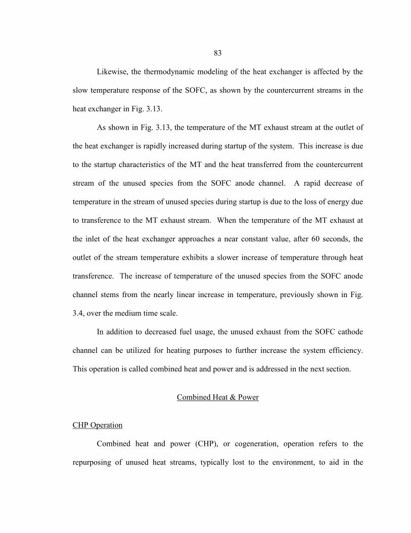
83

Likewise, the thermodynamic modeling of the heat exchanger is affected by the

slow temperature response of the SOFC, as shown by the countercurrent streams in the

heat exchanger in Fig. 3.13.

As shown in Fig. 3.13, the temperature of the MT exhaust stream at the outlet of

the heat exchanger is rapidly increased during startup of the system. This increase is due

to the startup characteristics of the MT and the heat transferred from the countercurrent

stream of the unused species from the SOFC anode channel. A rapid decrease of

temperature in the stream of unused species during startup is due to the loss of energy due

to transference to the MT exhaust stream. When the temperature of the MT exhaust at

the inlet of the heat exchanger approaches a near constant value, after 60 seconds, the

outlet of the stream temperature exhibits a slower increase of temperature through heat

transference. The increase of temperature of the unused species from the SOFC anode

channel stems from the nearly linear increase in temperature, previously shown in Fig.

3.4, over the medium time scale.

In addition to decreased fuel usage, the unused exhaust from the SOFC cathode

channel can be utilized for heating purposes to further increase the system efficiency.

This operation is called combined heat and power and is addressed in the next section.

Combined Heat & Power

CHP Operation

Combined heat and power (CHP), or cogeneration, operation refers to the

repurposing of unused heat streams, typically lost to the environment, to aid in the

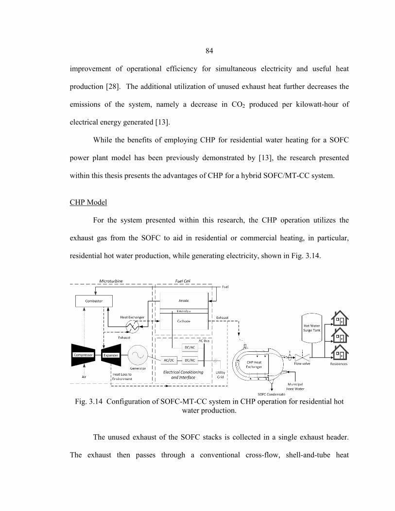
84

improvement of operational efficiency for simultaneous electricity and useful heat

production [28]. The additional utilization of unused exhaust heat further decreases the

emissions of the system, namely a decrease in CO2 produced per kilowatt-hour of

electrical energy generated [13].

While the benefits of employing CHP for residential water heating for a SOFC

power plant model has been previously demonstrated by [13], the research presented

within this thesis presents the advantages of CHP for a hybrid SOFC/MT-CC system.

CHP Model

For the system presented within this research, the CHP operation utilizes the

exhaust gas from the SOFC to aid in residential or commercial heating, in particular,

residential hot water production, while generating electricity, shown in Fig. 3.14.

Fig. 3.14 Configuration of SOFC-MT-CC system in CHP operation for residential hot

water production. The unused exhaust of the SOFC stacks is collected in a single exhaust header.

The exhaust then passes through a conventional cross-flow, shell-and-tube heat

85

exchanger. As the exhaust stream passes through the shell, heat is transferred to the

cooler inner tubing containing the residential hot water, causing an increase of

temperature in the water. The municipal water supply provides feed water to the cold

inlet of the heat exchanger, assumed to be a constant 13°C. The feed water circulates

around the heat exchanger tubing by the pressure maintained by the water utility, which

is between 40 and 80 psi. Exploiting the existing pressure of the feed water eliminates

the need for additional pumps. Once the SOFC exhaust has passed through the heat

exchanger and transferred heat to the residential hot water, it is released to the

environment at 200°C [13].

Although the SOFC/MT-CC system in CHP operation system is operated with a

utility grid interconnection, the research presented in this thesis focused on the ability of

the system to meet the power and hot water demands of a 250-home residential

neighborhood in the Pacific Northwest region of the United States.

Additional details regarding the CHP model can be found in [13].

Load Data

When appropriately sizing a system for a specific load, aggregate data directly

obtained from precise, real-time monitoring of the individual components that comprise

the system would ideally be used. However, this approach is not widely used for

residential load profiles. Consequently, the majority of residential load data currently

employed in research is found through an interpolation of a typical residence

configuration conjectured to suitably represent regional data, as opposed to direct

monitoring [45]-[47]. Recent research on optimal modeling for the residential sector has

86

aided the development of better techniques for obtaining residential end-use data [48].

Unfortunately, because much of the modeling methodology cannot yet be employed, an

alternative method to obtain relevant and accurate end-use profiles, developed by [49],

was utilized in this study. The data attained has been derived from the End-Use Load and

Consumer Assessment Program (ELCAP) studies completed in the 1990s, undertaken by

the Pacific Northwest Laboratory (PNNL) for Bonneville Power Administration (BPA)

and has been updated based on the most recent data available, specifically, 2010 EIA

base cases [50]. For this reason, it can be considered to be representative of the end use

curves for Pacific Northwest homes in the current era.

Fig. 3.15 Aggregated total residential electrical use seasonal profiles [49].

The aggregate end-use, time-of-day load curves based on seasonal usage patterns

in the Pacific Northwest region of the United States are shown in Fig. 3.15. The majority

87

of homes in the region observed utilized electric appliances, heating and ventilation, and

water heaters [49]. Fig. 3.15 shows the total aggregated end-use profiles for all-electric

residences, including an electric water heater (EWH). By assuming all-electric homes for

this study, the sizing of the generation system will be sufficient for a greatest electrical

load scenario.

While Fig. 3.15 provides the total electrical load profiles, it lacks EWH data

specific to water consumption. Therefore, the real-world residential hot water

consumption data representing the time-of-use average compiled by the American

Society of Heating, Refrigerating, and Air-Conditioning Engineers (ASHRAE) is utilized

and shown in Fig. 3.16 [51].

Fig. 3.16 ASHRAE residential hot water average consumption profile [51].

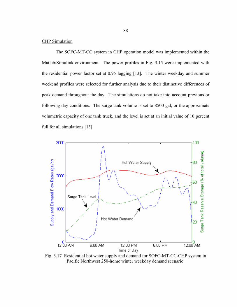
88

CHP Simulation

The SOFC-MT-CC system in CHP operation model was implemented within the

Matlab/Simulink environment. The power profiles in Fig. 3.15 were implemented with

the residential power factor set at 0.95 lagging [13]. The winter weekday and summer

weekend profiles were selected for further analysis due to their distinctive differences of

peak demand throughout the day. The simulations do not take into account previous or

following day conditions. The surge tank volume is set to 8500 gal, or the approximate

volumetric capacity of one tank truck, and the level is set at an initial value of 10 percent

full for all simulations [13].

Fig. 3.17 Residential hot water supply and demand for SOFC-MT-CC-CHP system in

Pacific Northwest 250-home winter weekday demand scenario.

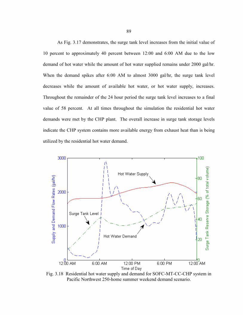
89

As Fig. 3.17 demonstrates, the surge tank level increases from the initial value of

10 percent to approximately 40 percent between 12:00 and 6:00 AM due to the low

demand of hot water while the amount of hot water supplied remains under 2000 gal/hr.

When the demand spikes after 6:00 AM to almost 3000 gal/hr, the surge tank level

decreases while the amount of available hot water, or hot water supply, increases.

Throughout the remainder of the 24 hour period the surge tank level increases to a final

value of 58 percent. At all times throughout the simulation the residential hot water

demands were met by the CHP plant. The overall increase in surge tank storage levels

indicate the CHP system contains more available energy from exhaust heat than is being

utilized by the residential hot water demand.

Fig. 3.18 Residential hot water supply and demand for SOFC-MT-CC-CHP system in

Pacific Northwest 250-home summer weekend demand scenario.

90

Fig. 3.18 demonstrates the summer weekend demand scenario, with a spike of

demand around 6:00 PM. Similar to the winter weekday scenario, the surge tank level

increases from the initial value of 10 percent to approximately 45 percent between 12:00

and 6:00 AM due to the low demand of hot water while the amount of hot water supplied

remains under 2000 gal/hr. The surge tank level decreases while the hot water supplied

increases when the demand spikes after 6:00 AM. Throughout the remainder of the 24

hour period the surge tank level increases to a final value of 56 percent. The difference

of tank levels for both scenario stems from the increased demand later in the day for the

summer weekend scenario. At all times throughout the simulation the residential hot

water demands were again met by the CHP plant. The overall increase in surge tank

storage level for both scenarios indicate the CHP system could be utilized for other

applications than the residential hot water demand for further cost savings [13].

Discussion

The CC chosen for this research is a variant of a Brayton cycle interconnection.

However, there are many other integration methods currently available when employing a

fuel cell and gas turbine [52]. Depending on the purpose and usage of the systems, the

interconnections can be reconfigured to produce greater efficiencies than those presented

in this research. The CC configuration within this research was deemed a common

coupling technique and thereby allows for future research to further improve the

efficiency of the system.

91

POWER MANAGEMENT OF SOFC-MT-CC SYSTEM The power management of the hybrid SOFC-MT-CC system is presented in this

chapter. A brief description of the power electronic interfaces, which connect to a

common bus, is also discussed.

The operation of the SOFC-MT-CC system is desired to be stable during transient

occurrences. Beside the advantage of increased efficiency, the coupling of a fuel cell

with a gas turbine also benefits in terms of transient stability and power management.

The electrochemical reactions that occur in a SOFC are slow in comparison to the

mechanical response of the MT. For this reason, during a transient period the fast

response of the MT is utilized for voltage and frequency stabilization and to prevent

damage occurring to the SOFC. For instance, rapid load fluctuations on a SOFC can

result in cell degradation of the SOFC, which can lead to thermal fatigue. In order to

prevent damage to the SOFC, the MT is given the responsibility of responding to

transient events to maintain the voltage and frequency of the system.

System Overview

The hybrid SOFC-MT-CC system presented in Chapter 3 (see Fig. 3.1) consists of

models for the SOFC, MT, heat exchanger, combustor, and power electronics interfacing.

The power electronics interfacing is connected to an AC bus which supplies an AC load.

In the following section, a brief description of the power electronics interfacing is given

[53].

92

Power Electronics Interfacing

Power electronics (PE) interfacing are necessary for hybrid systems to maintain

the output voltage and frequency of each generating component of the system. The PE

interfacing used for the hybrid system consists of a DC/DC boost converter and DC/AC

inverter for the SOFC and an AC/DC rectifier and DC/AC inverter for the MT. The PE

interfacing is used to control the real and reactive power by controlling the inverter

output voltage angle, and frequency. The SOFC and MT each contain their own dq

transformed PE interface. Further details of the PE interfaces and their subsequent

implementation can be found in [4], [6], [53].

Simulation Results

The simulation of a stand-alone MT, a stand-alone SOFC, and the SOFC-MT-CC

system were conducted. In each case, a variable load was attached to record the load

response capabilities of each generation source.

MT Response to Variable Load

The load response of the MT was first analyzed in order to determine the amount

of time required to return to a steady state. A variable load was attached to the MT, as

shown in Fig. 4.1. The variable load begins at 250 kW from t = 0 to 20 s, then the load

decreases to 150 kW from t = 20 to 30 s; it then increases to 200 kW from t = 30 to 40 s.

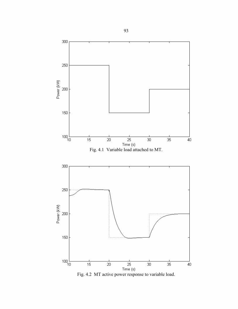
93

Fig. 4.1 Variable load attached to MT.

Fig. 4.2 MT active power response to variable load.

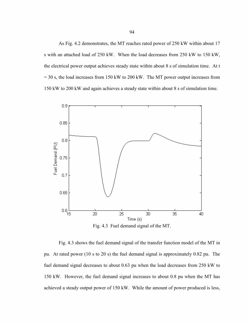
94

As Fig. 4.2 demonstrates, the MT reaches rated power of 250 kW within about 17

s with an attached load of 250 kW. When the load decreases from 250 kW to 150 kW,

the electrical power output achieves steady state within about 8 s of simulation time. At t

= 30 s, the load increases from 150 kW to 200 kW. The MT power output increases from

150 kW to 200 kW and again achieves a steady state within about 8 s of simulation time.

Fig. 4.3 Fuel demand signal of the MT.

Fig. 4.3 shows the fuel demand signal of the transfer function model of the MT in

pu. At rated power (10 s to 20 s) the fuel demand signal is approximately 0.82 pu. The

fuel demand signal decreases to about 0.63 pu when the load decreases from 250 kW to

150 kW. However, the fuel demand signal increases to about 0.8 pu when the MT has

achieved a steady output power of 150 kW. While the amount of power produced is less,

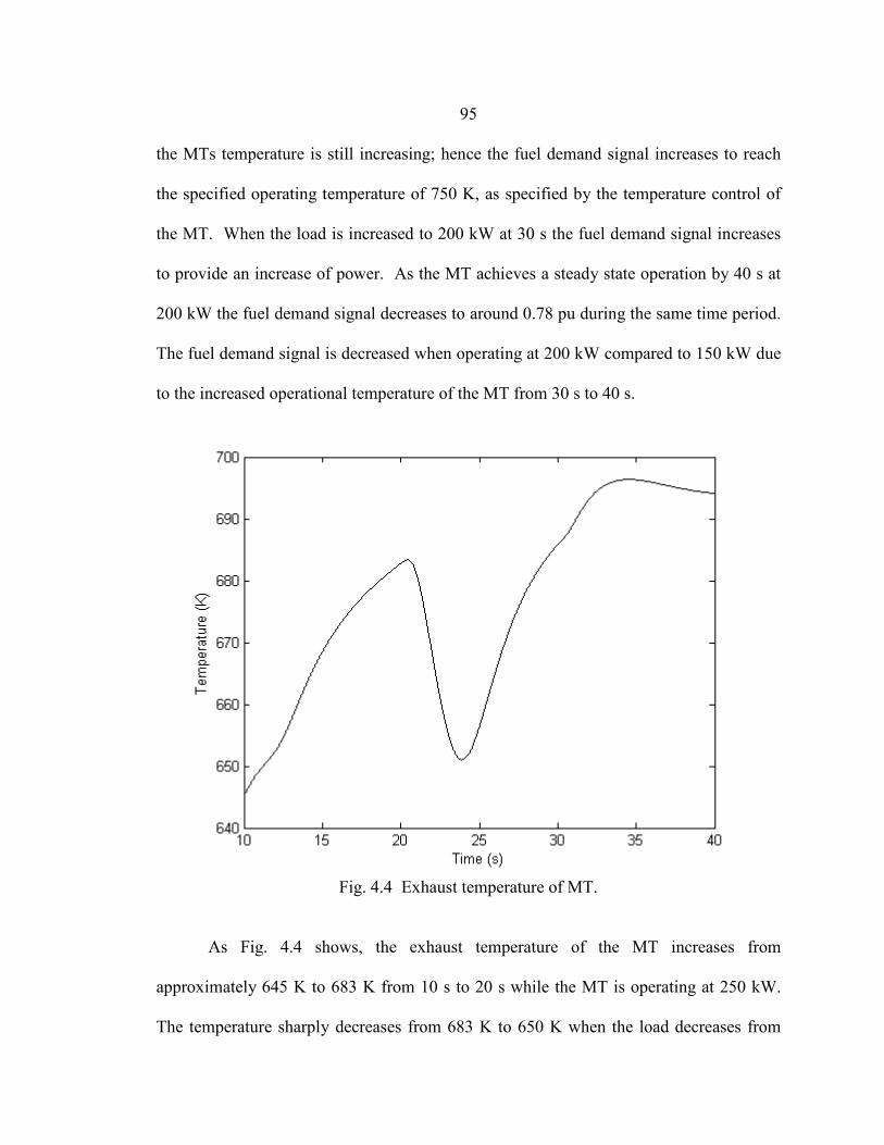
95

the MTs temperature is still increasing; hence the fuel demand signal increases to reach

the specified operating temperature of 750 K, as specified by the temperature control of

the MT. When the load is increased to 200 kW at 30 s the fuel demand signal increases

to provide an increase of power. As the MT achieves a steady state operation by 40 s at

200 kW the fuel demand signal decreases to around 0.78 pu during the same time period.

The fuel demand signal is decreased when operating at 200 kW compared to 150 kW due

to the increased operational temperature of the MT from 30 s to 40 s.

Fig. 4.4 Exhaust temperature of MT.

As Fig. 4.4 shows, the exhaust temperature of the MT increases from

approximately 645 K to 683 K from 10 s to 20 s while the MT is operating at 250 kW.

The temperature sharply decreases from 683 K to 650 K when the load decreases from

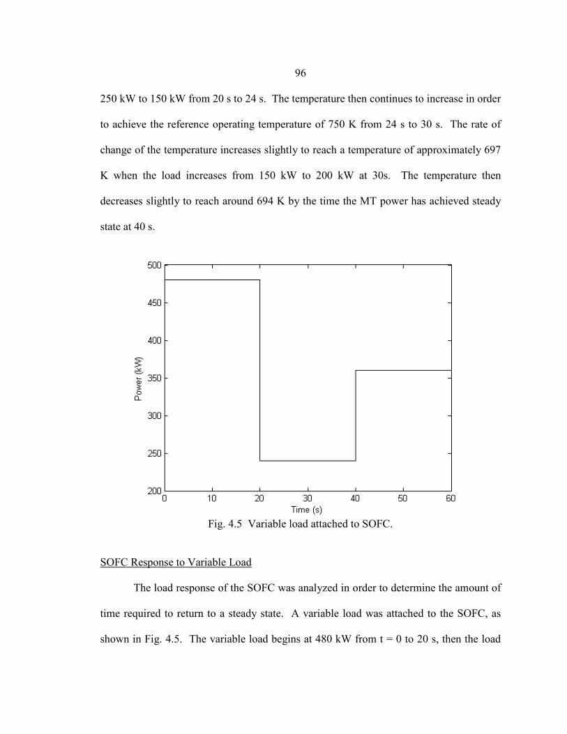
96

250 kW to 150 kW from 20 s to 24 s. The temperature then continues to increase in order

to achieve the reference operating temperature of 750 K from 24 s to 30 s. The rate of

change of the temperature increases slightly to reach a temperature of approximately 697

K when the load increases from 150 kW to 200 kW at 30s. The temperature then

decreases slightly to reach around 694 K by the time the MT power has achieved steady

state at 40 s.

Fig. 4.5 Variable load attached to SOFC.

SOFC Response to Variable Load

The load response of the SOFC was analyzed in order to determine the amount of

time required to return to a steady state. A variable load was attached to the SOFC, as

shown in Fig. 4.5. The variable load begins at 480 kW from t = 0 to 20 s, then the load

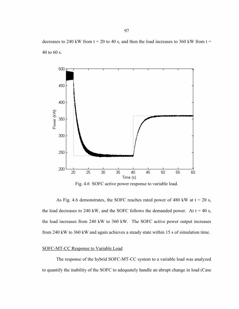
97

decreases to 240 kW from t = 20 to 40 s, and then the load increases to 360 kW from t =

40 to 60 s.

Fig. 4.6 SOFC active power response to variable load.

As Fig. 4.6 demonstrates, the SOFC reaches rated power of 480 kW at t = 20 s,

the load decreases to 240 kW, and the SOFC follows the demanded power. At t = 40 s,

the load increases from 240 kW to 360 kW. The SOFC active power output increases

from 240 kW to 360 kW and again achieves a steady state within 15 s of simulation time.

SOFC-MT-CC Response to Variable Load

The response of the hybrid SOFC-MT-CC system to a variable load was analyzed

to quantify the inability of the SOFC to adequately handle an abrupt change in load (Case

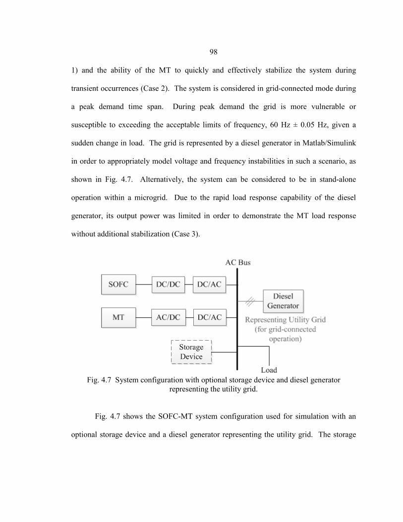
98

1) and the ability of the MT to quickly and effectively stabilize the system during

transient occurrences (Case 2). The system is considered in grid-connected mode during

a peak demand time span. During peak demand the grid is more vulnerable or

susceptible to exceeding the acceptable limits of frequency, 60 Hz ± 0.05 Hz, given a

sudden change in load. The grid is represented by a diesel generator in Matlab/Simulink

in order to appropriately model voltage and frequency instabilities in such a scenario, as

shown in Fig. 4.7. Alternatively, the system can be considered to be in stand-alone

operation within a microgrid. Due to the rapid load response capability of the diesel

generator, its output power was limited in order to demonstrate the MT load response

without additional stabilization (Case 3).

Fig. 4.7 System configuration with optional storage device and diesel generator

representing the utility grid. Fig. 4.7 shows the SOFC-MT system configuration used for simulation with an

optional storage device and a diesel generator representing the utility grid. The storage

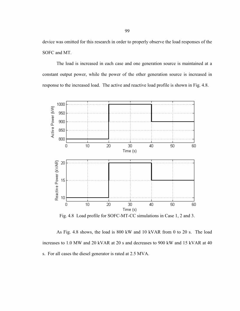
99

device was omitted for this research in order to properly observe the load responses of the

SOFC and MT.

The load is increased in each case and one generation source is maintained at a

constant output power, while the power of the other generation source is increased in

response to the increased load. The active and reactive load profile is shown in Fig. 4.8.

Fig. 4.8 Load profile for SOFC-MT-CC simulations in Case 1, 2 and 3.

As Fig. 4.8 shows, the load is 800 kW and 10 kVAR from 0 to 20 s. The load

increases to 1.0 MW and 20 kVAR at 20 s and decreases to 900 kW and 15 kVAR at 40

s. For all cases the diesel generator is rated at 2.5 MVA.

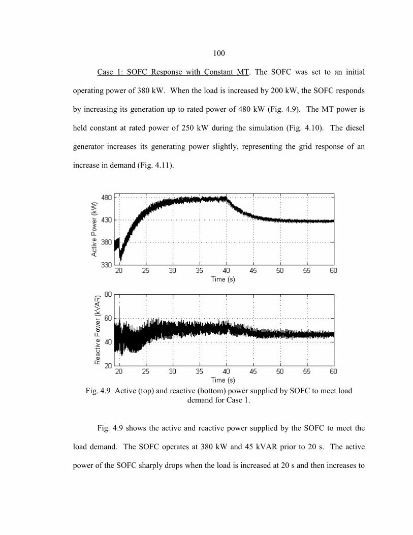
100

Case 1: SOFC Response with Constant MT

Fig. 4.9

. The SOFC was set to an initial

operating power of 380 kW. When the load is increased by 200 kW, the SOFC responds

by increasing its generation up to rated power of 480 kW ( ). The MT power is

held constant at rated power of 250 kW during the simulation (Fig. 4.10). The diesel

generator increases its generating power slightly, representing the grid response of an

increase in demand (Fig. 4.11).

Fig. 4.9 Active (top) and reactive (bottom) power supplied by SOFC to meet load

demand for Case 1. Fig. 4.9 shows the active and reactive power supplied by the SOFC to meet the

load demand. The SOFC operates at 380 kW and 45 kVAR prior to 20 s. The active

power of the SOFC sharply drops when the load is increased at 20 s and then increases to

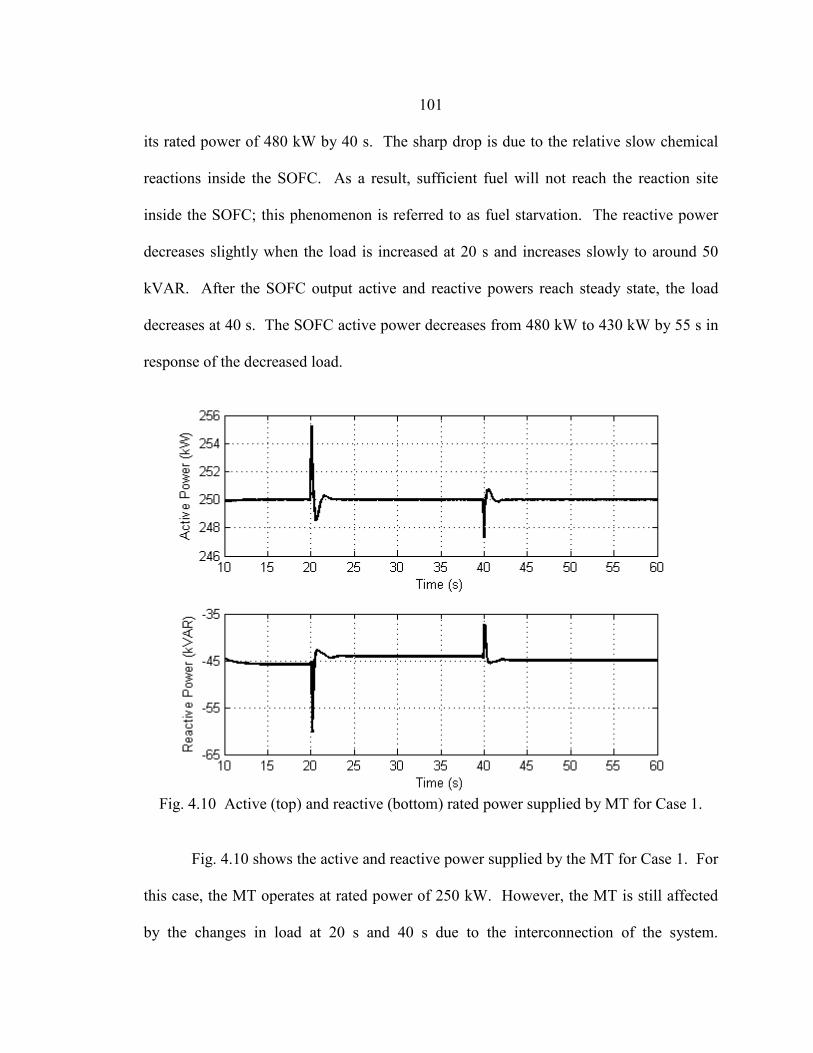
101

its rated power of 480 kW by 40 s. The sharp drop is due to the relative slow chemical

reactions inside the SOFC. As a result, sufficient fuel will not reach the reaction site

inside the SOFC; this phenomenon is referred to as fuel starvation. The reactive power

decreases slightly when the load is increased at 20 s and increases slowly to around 50

kVAR. After the SOFC output active and reactive powers reach steady state, the load

decreases at 40 s. The SOFC active power decreases from 480 kW to 430 kW by 55 s in

response of the decreased load.

Fig. 4.10 Active (top) and reactive (bottom) rated power supplied by MT for Case 1.

Fig. 4.10 shows the active and reactive power supplied by the MT for Case 1. For

this case, the MT operates at rated power of 250 kW. However, the MT is still affected

by the changes in load at 20 s and 40 s due to the interconnection of the system.

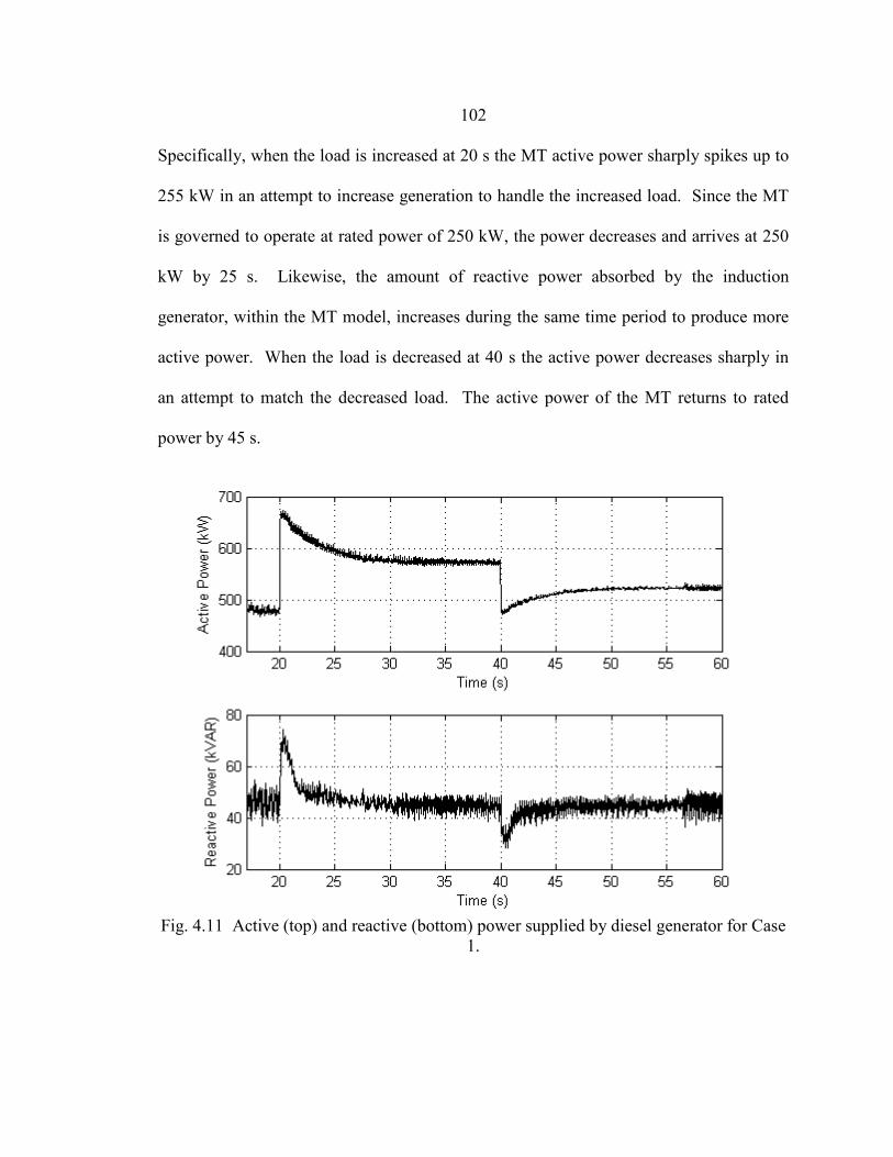
102

Specifically, when the load is increased at 20 s the MT active power sharply spikes up to

255 kW in an attempt to increase generation to handle the increased load. Since the MT

is governed to operate at rated power of 250 kW, the power decreases and arrives at 250

kW by 25 s. Likewise, the amount of reactive power absorbed by the induction

generator, within the MT model, increases during the same time period to produce more

active power. When the load is decreased at 40 s the active power decreases sharply in

an attempt to match the decreased load. The active power of the MT returns to rated

power by 45 s.

Fig. 4.11 Active (top) and reactive (bottom) power supplied by diesel generator for Case

1.

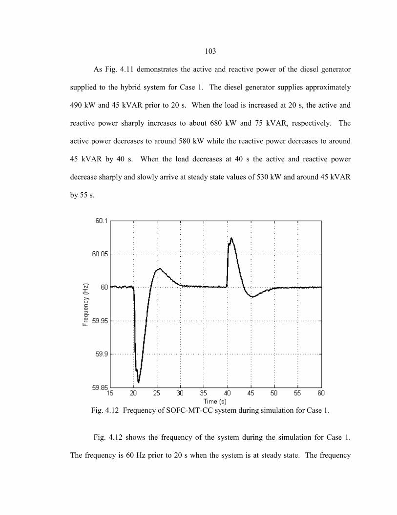
103

As Fig. 4.11 demonstrates the active and reactive power of the diesel generator

supplied to the hybrid system for Case 1. The diesel generator supplies approximately

490 kW and 45 kVAR prior to 20 s. When the load is increased at 20 s, the active and

reactive power sharply increases to about 680 kW and 75 kVAR, respectively. The

active power decreases to around 580 kW while the reactive power decreases to around

45 kVAR by 40 s. When the load decreases at 40 s the active and reactive power

decrease sharply and slowly arrive at steady state values of 530 kW and around 45 kVAR

by 55 s.

Fig. 4.12 Frequency of SOFC-MT-CC system during simulation for Case 1.

Fig. 4.12 shows the frequency of the system during the simulation for Case 1.

The frequency is 60 Hz prior to 20 s when the system is at steady state. The frequency

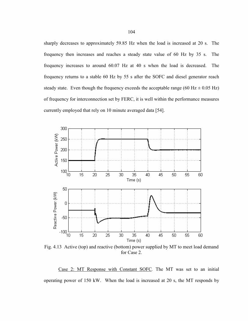
104

sharply decreases to approximately 59.85 Hz when the load is increased at 20 s. The

frequency then increases and reaches a steady state value of 60 Hz by 35 s. The

frequency increases to around 60.07 Hz at 40 s when the load is decreased. The

frequency returns to a stable 60 Hz by 55 s after the SOFC and diesel generator reach

steady state. Even though the frequency exceeds the acceptable range (60 Hz ± 0.05 Hz)

of frequency for interconnection set by FERC, it is well within the performance measures

currently employed that rely on 10 minute averaged data [54].

Fig. 4.13 Active (top) and reactive (bottom) power supplied by MT to meet load demand

for Case 2. Case 2: MT Response with Constant SOFC. The MT was set to an initial

operating power of 150 kW. When the load is increased at 20 s, the MT responds by

105

increasing its generation up to rated power of 250 kW. The diesel generator responds by

increasing supplied power slightly, as occurred in Case 1. The SOFC power is held

constant at rated power of 480 kW during the simulation.

Fig. 4.13 shows the active and reactive power supplied by the MT to meet the

load demand. The active power of the MT increases from 150 kW to 250 kW within 5 s

after the load is increased at 20 s. The reactive power of the MT decreases during the

same time period, or becomes more negative. Since the negative sign denotes absorption

of power, or power flowing into the measurement reference, the reactive power of the

induction generator can be equivalently described as an increase of reactive power

absorbed. When the load current is increased in a system with a fixed reactive power

supply, the terminal voltage of the induction generator will decrease. In order to

compensate, or increase the voltage, additional reactive power is required by the

induction generator [55]. In this system, the additional reactive power is supplied by the

grid, represented by the diesel generator. Also, the reactive power losses are increased

due to the increased current. In order for the induction generator to increase active power

output, the reactive power must be increased into the device. After the MT output active

and reactive power stabilizes at 250 kW and -50 kVAR, respectively, the load decreases

at 40 s. The MT active power decreases from 250 kW to 200 kW from 40 to 45 s in

response to the decrease of load.

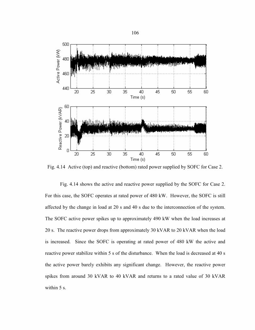
106

Fig. 4.14 Active (top) and reactive (bottom) rated power supplied by SOFC for Case 2.

Fig. 4.14 shows the active and reactive power supplied by the SOFC for Case 2.

For this case, the SOFC operates at rated power of 480 kW. However, the SOFC is still

affected by the change in load at 20 s and 40 s due to the interconnection of the system.

The SOFC active power spikes up to approximately 490 kW when the load increases at

20 s. The reactive power drops from approximately 30 kVAR to 20 kVAR when the load

is increased. Since the SOFC is operating at rated power of 480 kW the active and

reactive power stabilize within 5 s of the disturbance. When the load is decreased at 40 s

the active power barely exhibits any significant change. However, the reactive power

spikes from around 30 kVAR to 40 kVAR and returns to a rated value of 30 kVAR

within 5 s.

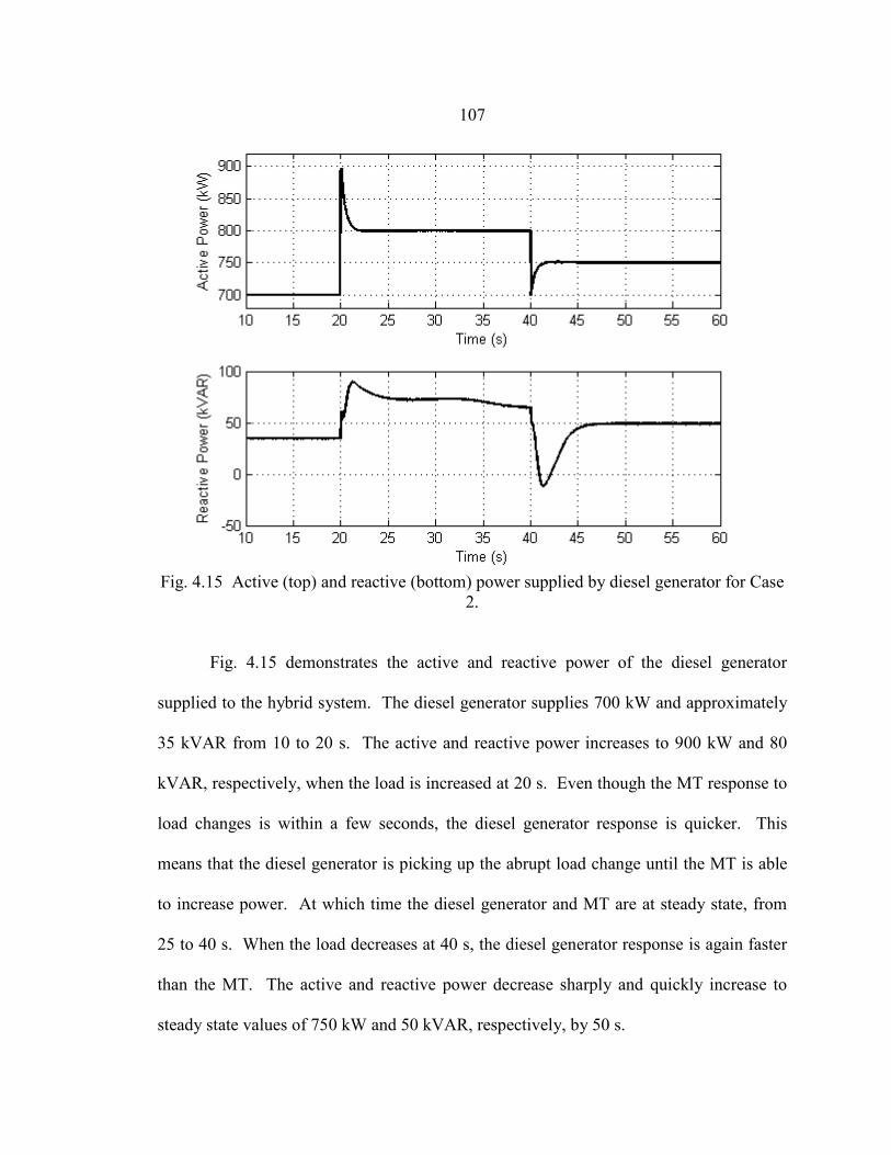
107

Fig. 4.15 Active (top) and reactive (bottom) power supplied by diesel generator for Case

2. Fig. 4.15 demonstrates the active and reactive power of the diesel generator

supplied to the hybrid system. The diesel generator supplies 700 kW and approximately

35 kVAR from 10 to 20 s. The active and reactive power increases to 900 kW and 80

kVAR, respectively, when the load is increased at 20 s. Even though the MT response to

load changes is within a few seconds, the diesel generator response is quicker. This

means that the diesel generator is picking up the abrupt load change until the MT is able

to increase power. At which time the diesel generator and MT are at steady state, from

25 to 40 s. When the load decreases at 40 s, the diesel generator response is again faster

than the MT. The active and reactive power decrease sharply and quickly increase to

steady state values of 750 kW and 50 kVAR, respectively, by 50 s.

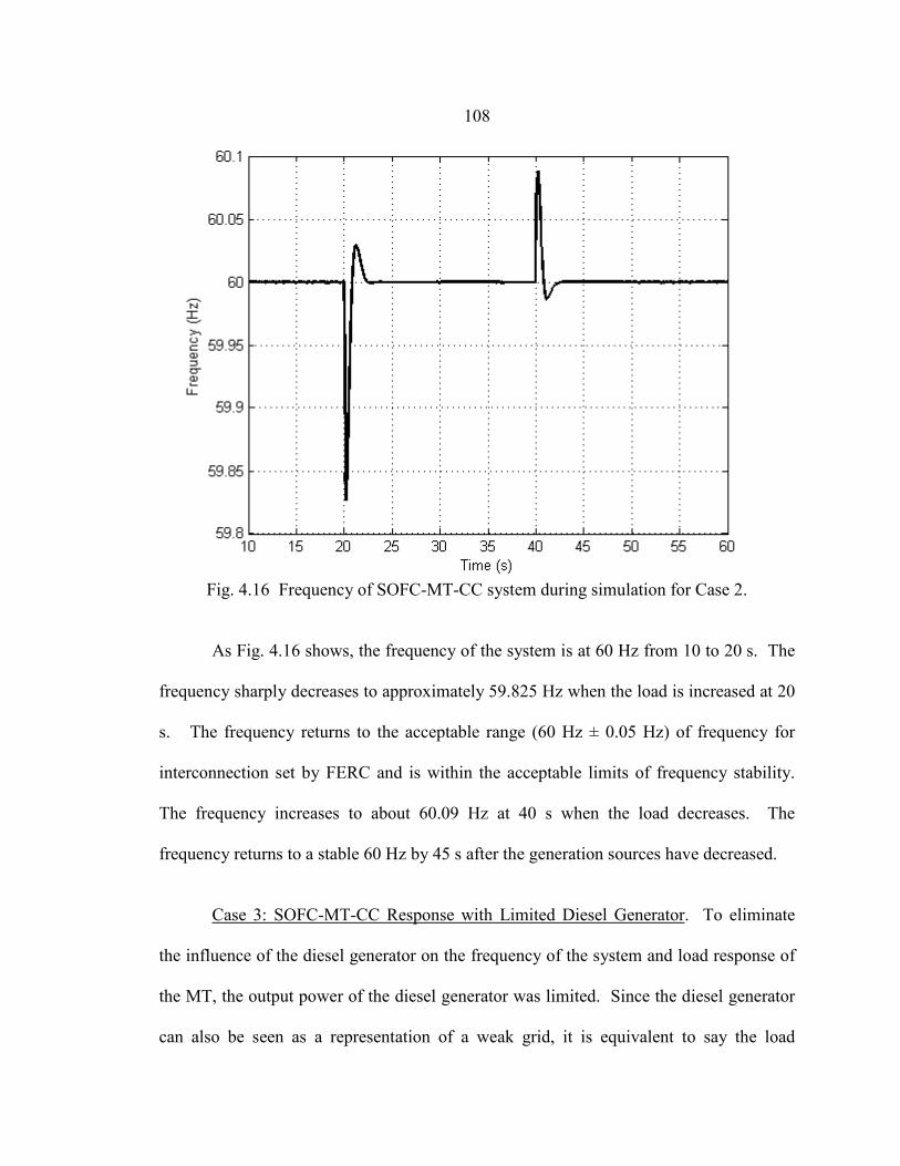
108

Fig. 4.16 Frequency of SOFC-MT-CC system during simulation for Case 2.

As Fig. 4.16 shows, the frequency of the system is at 60 Hz from 10 to 20 s. The

frequency sharply decreases to approximately 59.825 Hz when the load is increased at 20

s. The frequency returns to the acceptable range (60 Hz ± 0.05 Hz) of frequency for

interconnection set by FERC and is within the acceptable limits of frequency stability.

The frequency increases to about 60.09 Hz at 40 s when the load decreases. The

frequency returns to a stable 60 Hz by 45 s after the generation sources have decreased.

Case 3: SOFC-MT-CC Response with Limited Diesel Generator. To eliminate

the influence of the diesel generator on the frequency of the system and load response of

the MT, the output power of the diesel generator was limited. Since the diesel generator

can also be seen as a representation of a weak grid, it is equivalent to say the load

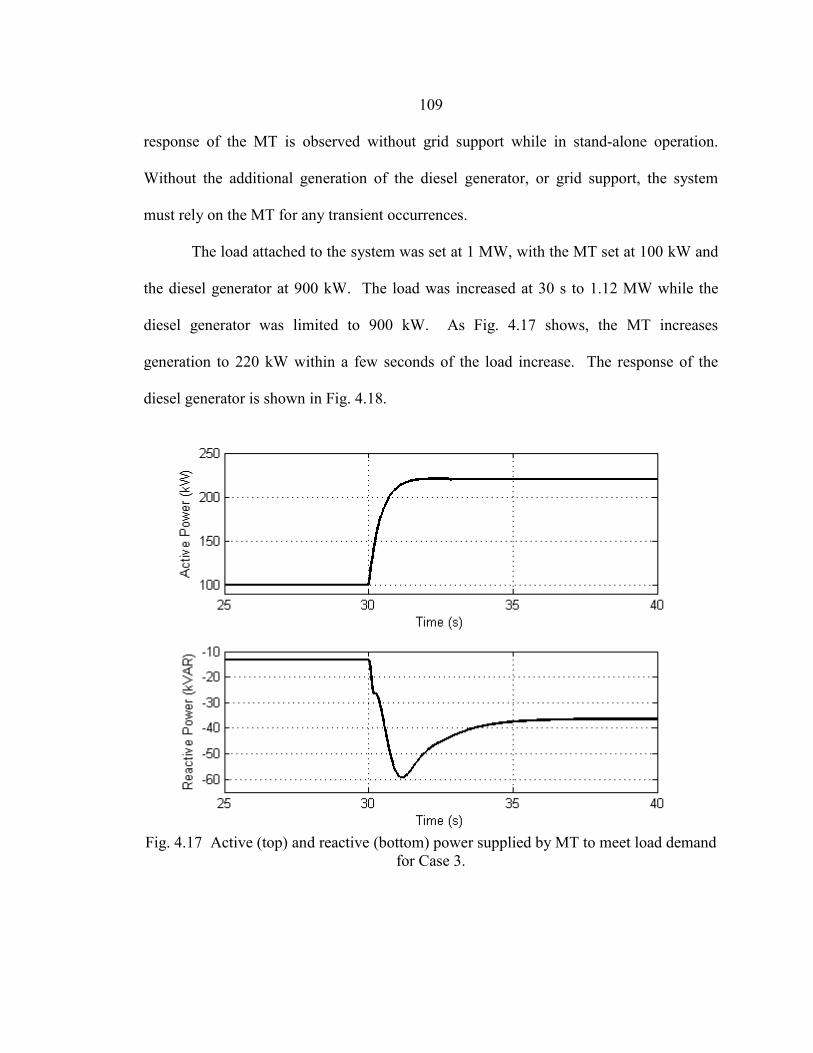
109

response of the MT is observed without grid support while in stand-alone operation.

Without the additional generation of the diesel generator, or grid support, the system

must rely on the MT for any transient occurrences.

The load attached to the system was set at 1 MW, with the MT set at 100 kW and

the diesel generator at 900 kW. The load was increased at 30 s to 1.12 MW while the

diesel generator was limited to 900 kW. As Fig. 4.17 shows, the MT increases

generation to 220 kW within a few seconds of the load increase. The response of the

diesel generator is shown in Fig. 4.18.

Fig. 4.17 Active (top) and reactive (bottom) power supplied by MT to meet load demand

for Case 3.

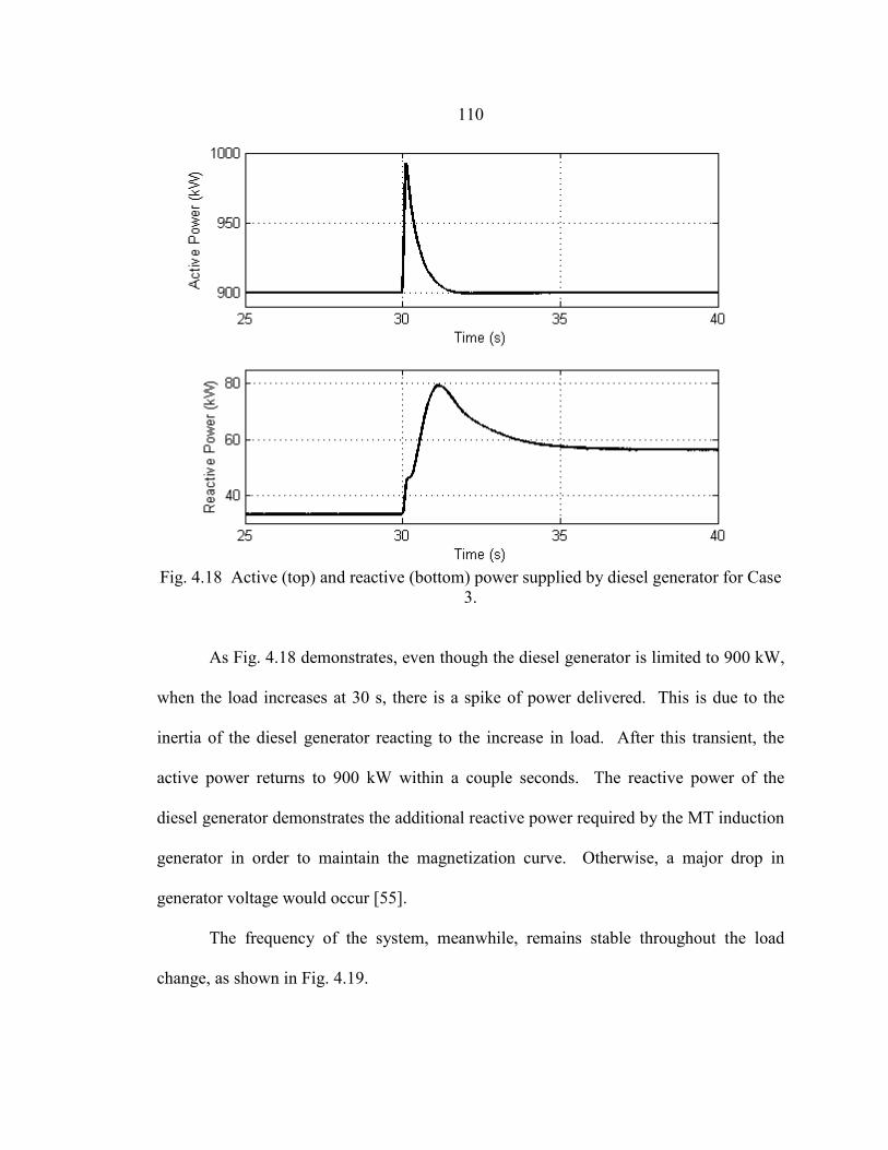
110

Fig. 4.18 Active (top) and reactive (bottom) power supplied by diesel generator for Case

3. As Fig. 4.18 demonstrates, even though the diesel generator is limited to 900 kW,

when the load increases at 30 s, there is a spike of power delivered. This is due to the

inertia of the diesel generator reacting to the increase in load. After this transient, the

active power returns to 900 kW within a couple seconds. The reactive power of the

diesel generator demonstrates the additional reactive power required by the MT induction

generator in order to maintain the magnetization curve. Otherwise, a major drop in

generator voltage would occur [55].

The frequency of the system, meanwhile, remains stable throughout the load

change, as shown in Fig. 4.19.

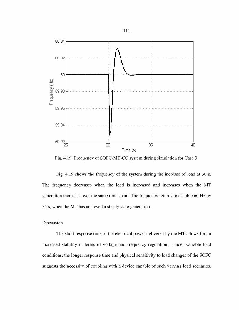
111

Fig. 4.19 Frequency of SOFC-MT-CC system during simulation for Case 3.

Fig. 4.19 shows the frequency of the system during the increase of load at 30 s.

The frequency decreases when the load is increased and increases when the MT

generation increases over the same time span. The frequency returns to a stable 60 Hz by

35 s, when the MT has achieved a steady state generation.

Discussion

The short response time of the electrical power delivered by the MT allows for an

increased stability in terms of voltage and frequency regulation. Under variable load

conditions, the longer response time and physical sensitivity to load changes of the SOFC

suggests the necessity of coupling with a device capable of such varying load scenarios.

112

In this sense, a MT is capable and suited well to pair with a SOFC given its fast

mechanical operation.

In order for the system to aptly respond to all transient events a fast-response

energy storage device along with a proper power management strategy is required, and is

recommended for fuel cell hybrid systems.

113

CONCLUSION

Hybrid SOFC-MT systems benefit from combined cycle operation by increasing

the efficiency and transient capabilities of the system along with decreasing fuel

consumption and subsequent emissions. This research considered the modeling,

efficiency evaluation, and power management of a hybrid SOFC-MT system in combined

cycle (CC) operation with combined heat and power (CHP) functionality for residential

applications in islanded or grid-connected modes within a microgrid environment. The

MT exhaust gas stream and the unused SOFC fuel stream from the anode channel were

utilized in CC operation preheat the fuel in the MT for an increase of efficiency. The

efficiency of the system was analyzed through the interconnection of a transfer function

and thermodynamic microturbine model. The modeling of thermodynamically based

combustor and heat exchanger models was also presented. The exhaust gas from the

SOFC was utilized in CHP operation for residential hot water and electricity production

for 250 residences in the Pacific Northwest. The load response of the SOFC and MT

were also examined during transient load events. The SOFC was shown to have a slower

response than the MT to load changes. The hybrid system frequency was also shown to

remain stable during load transients in a microgrid environment.

Future Work

SOFC-MT hybrids have a great potential to function as effective electricity

sources for the future, while more efficient fuels, i.e. hydrogen, can subsequently be

integrated into the SOFC-MT installations, further improving generation efficiency and

114

lowering associated costs. The addition of renewable energy sources, such as a wind or

PV, to the SOFC-MT-CC system can be further analyzed as a DG source. By increasing

the number of generation sources, the system will be more robust, yet require further

control and power management strategies to be employed. A cost benefit analysis as well

as a stability analysis can also be conducted on a system with more generation sources.

115

REFERENCES CITED [1] IEEE Standard for Interconnecting Distributed Resources with Electric Power

Systems, IEEE Standard 1547-2003, 2003.

[2] "Grid Reliability and Power Quality Impacts of Distributed Resources," EPRI, Palo Alto, CA, 2003.1004473.

[3] Fuel Cell Handbook, 7th ed., EG&G Services, Inc.; DOE, Office of Fossil Energy, National Energy Technology Laboratory, 2004.

[4] M. H. Nehrir and C. Wang, Modeling and Control of Fuel Cells, Hoboken, NJ: Wiley-IEEE Press, 2009.

[5] J. Larminie and A. Dicks, Fuel Cell Systems Explained, 2nd ed., Hoboken, NJ: Wiley, 2003.

[6] S. R. Guda, C. Wang and M. H. Nehrir, "Modeling of Microturbine Power Generation Systems," Electric Power Components and Systems, vol. 34, pp. 1027-1041, 2006.

[7] L. Goldstein, B. Hedman, D. Knowles, S. I. Freedman, R. Woods and T. Schweizer, "Gas-Fired Distributed Energy Resource Technology Characterizations," National Renewable Energy Laboratory, NREL/TP-620-34783, Nov. 2003.

[8] A. K. Saha, S. Chowdhury and P. A. Crossley, "Modeling and Performance Analysis of a Microturbine as a Distributed Energy Resource," IEEE Trans. Energy Convers., vol. 24, no. 2, pp. 529-538, June 2009.

[9] E. Achenbach, "Response of a solid oxide fuel cell to load change," J. Power Sources, vol. 57, no. 1, pp. 105-109, 1995.

[10] C. Wang and M. H. Nehrir, "Short-Time Overloading Capability and Distributed Generation Applications of Solid Oxide Fuel Cells," IEEE Trans. Energy Convers., vol. 22, no. 4, pp. 898-906, Dec. 2007.

[11] S. Singhal, "Solid oxide fuel cells for stationary, mobile, and military applications," Solid State Ionics 152-153, pp. 405-410, 2002.

116

[12] Y. Haseli, I. Dincer and G. F. Naterer, "Thermodynamic modeling of a gas turbine cycle combined with a solid oxide fuel cell," Int. J. Hydrogen Energy, no. 33, pp. 5811-5822, 2008.

[13] C. M. Colson and M. H. Nehrir, "Evaluating the Benefits of a Hybrid Solid Oxide Fuel Cell Combined Head & Power Plant for Energy Sustainability and Emissions Avoidance," IEEE Trans. Energy Convers., vol. 26, no. 1, pp. 140-148, March 2011.

[14] F. Jurado and J. R. Saenz, "Adaptive Control of a Fuel Cell-Microturbine Hybrid Power Plant," IEEE Trans. on Energy Convers., vol. 18, no. 2, pp. 342-347, June 2003.

[15] S. K. Park, K. S. Oh and T. S. Kim, "Analysis of the design of a pressurized SOFC hybrid system using a fixed gas turbine design," J. Power Sources, vol. 170, pp. 130-139, 2007.

[16] R. U. Ayres, H. Turton and T. Casten, "Energy efficiency, sustainability, and economic growth," Energy, vol. 32, no. 5, May 2007.

[17] R. U. Ayres, L. W. Ayres and B. Warr, "Exergy, power and work in the US economy, 1900-1998," Energy, vol. 32, no. 5, March 2003.

[18] W. Graus and E. Worrell, "Trend in efficiency and capacity of fossil power generation in the EU," Energy Policy, vol. 37, no. 6, June 2009.

[19] Y. Zhu and K. Tomsovic, “Development of models for anlyzing the load-following performance of microturbines and fuel cells,” Electric Power Syst. Research, vol 62, pp. 1-11, 2002.

[20] N. Autissier, F. Palazzi, F. Marechal, J. van Herle and D. Favrat, “Thermo-Economic Optimization of a Solid Oxide Fuel Cell, Gas Turbine Hybrid System,” J. Fuel Cell Sci. Technol., vol. 4, pp. 123-129, May 2007.

[21] M. Granovskii, I. Dincer and M. A. Rosen, “Performance comparison of two combined SOFC-gas turbine systems,” J. Power Sources, vol. 165, pp. 307-314, 2007.

[22] S. K. Yee, J. V. Milanovic and F. M. Hughes, "Overview and Comparative Analysis of Gas Turbine Models for System Stability Studies," IEEE Trans. Power Syst., vol. 23, no. 1, pp. 108-118, February 2008.

117

[23] M. A. El-Masri, “A Modified, High-Efficiency, Recuperated Gas Turbine Cycle,” J. Eng. Gas Turbines Power, vol. 110, no. 2, pp. 233-243, April 1988.

[24] C. Wang and M. H. Nehrir, "A Physically Based Dynamic Model for Solid Oxide Fuel Cells," IEEE Trans. Energy Convers., vol. 22, no. 4, pp. 887-897, 2007.

[25] C. Colson, M. Nehrir, M. Deibert, M. Amin and C. Wang, "Efficiency Evaluation of Solid-Oxide Fuel Cells in Combined Cycle Operations," J. Fuel Cell Sci. Technol., vol. 6, pp. 1-6, May 2009.

[26] C. M. Colson, M. H. Nehrir and C. Wang, "Modeling a large-scale utility-interconnected solid oxide fuel cell power plant," in Proc. 40th North American Power Symp., Calgary, AB, Canada, 2008.

[27] G. M. Masters, Renewable and Efficient Electric Power Systems, Hoboken, New Jersey: Wiley, 2004, p. 170.

[28] Y. A. Cengel and M. A. Boles, Thermodynamics: An Engineering Approach, 6th ed., New York, NY: McGraw-Hill, 2008.

[29] W. E. Forsthoffer, Forsthoffer's Rotating Equipment Handbooks: Principles of Rotating Equipment, Elsevier, 2006.

[30] J. D. Glover, M. S. Sarma and T. J. Overbye, Power System Analysis and Design, Thomson, 2008.

[31] S. A. Pourmousavi, M. H. Nehrir, C. M. Colson and C. Wang, "Real-Time Energy Management of a Stand-Alone Wind-Microturbine Energy System Using Particle Swarm Optimization," IEEE Trans. Sustainable Energy, vol. 1, no. 3, pp. 193-201, Oct. 2010.

[32] W. I. Rowen, "Simplified mathematical representations of heavy duty gas turbines," J. Eng Power Trans. ASME, vol. 105, no. 4, pp. 865-869, October 1983.

[33] F. Jurado and A. Cano, "Use of ARX algorithms for modeling micro-turbines on the distribution feeder," Proc. IEEE Gen. Trans. Dist., vol. 151, no. 2, pp. 232-238, March 2004.

[34] L. N. Hannet and K. A., "Combustion turbine dynamic model validation from tests," IEEE Trans. Power Syst., vol. 8, no. 1, pp. 152-158, February 1993.

[35] S. R. Turns, An Introduction to Combustion: Concepts & Applications, 2nd ed., McGraw-Hill, 1999.

118

[36] Nat. Inst. of Standards and Technol., NIST Chemistry WebBook, NIST Standard Reference Database Number 69, P. J. Linstrom and W. G. Mallard, Eds., Gaithersburg, MD: Nat. Inst. of Standards and Technol., 2009.

[37] J. Senft, Mechanical Efficiency of Heat Engines, New York, NY: Cambridge University Press, 2007.

[38] "Assessment of Leading Microturbine Technologies," EPRI, Palo Alto, CA, 2003.1004454.

[39] C. Fannin, "Linear Modeling and Analysis of Thermoacoustic Instabilities in a Gas Turbine Combustor," Ph.D. dissertation, Dept. Mech. Eng., Virginia Polytechnic Inst., Blacksburg, VA, 2000.

[40] T. Kaneko, J. Brower and G. S. Samuelsen, "Power and temperature control of fluctuating biomass gas fueled solid oxide fuel cell and micro gas turbine hybrid system," J. Power Sources, vol. 160, pp. 316-325, 2006.

[41] A. Bejan and A. D. Kraus, Heat Transfer Handbook, Vol. 1, Wiley-IEEE Press, 2003.

[42] Trax Corp., ProTrax Programmer's Manual, TRAX Int., Forest, VA, 1998.

[43] ASM Int. Materials Properties Database Committee, ASM Ready Reference: Thermal Properties of Metals, ASM Int., 2002.

[44] I. Glassman and R. A. Yetter, Combustion, Burlington, MA, Academic Press, 2008.

[45] S. Heunis and R. Herman, “A probabillistic model for residential consumer loads,” IEEE Trans. Power Syst., vol. 17, no. 3, Aug. 2002.

[46] R. T. Guttromson, D. P. Chassin, and S. E. Widergren, “Residential energy resource models for distribution feeder simulation,” 2003 IEEE PES General Meeting Proc., vol. 1, July 2003.

[47] D. McQueen, P. Hyland, and S. Watson, “Monte Carlo simulation of residential electricity demand for forecasting maximum demand on distribution networks,” IEEE Trans. Power Syst., vol. 19, no. 3, Aug. 2004.

[48] L. G. Swan and V. I. Ugursal, “Modeling of end-use energy consumption in the residential sector: A review of modeling techniques,” Renewable and Sustainable Energy Reviews, no. 13, pp. 1819-1835, 2009.

119

[49] C. Colson and M. H. Nehrir, “An Alternative Method to Load Modeling for Obtaining End-Use Load Profiles,” in Proc. 41st North American Power Symp., Starksville, MS, Oct. 2009.

[50] Energy Inform. Admin., “Annu. Energy Review 2010,” U.S. DOE, Oct. 2011. [Online], Available: http://www.eia.doe.gov/aer

[51] B. R. Becker and K. E. Stogsdill, “A domestic hot water use database,” J. Amer. Soc. Heating, Refrigeration, Air-Conditioning Engineers (ASHRAE), vol. 32, no. 9, pp. 21-25, 1990.

[52] X. Zhang, S. H. Chan, L. Guojun, H. K. Ho, J. Li, Z. Feng, “A review of integration strategies for solid oxide fuel cells,” J. Power Sources, vol. 195, pp. 685-702, 2010 .

[53] C. Wang, “Modeling and Power Management of Hybrid Wind/Photovoltaic/Fuel Cell Distributed Generation System,” Ph.D. dissertation, Dept. Elec. Eng., Montana State Univ., Bozeman, MT, 2006.

[54] H. F. Illian, “Frequency Control Performance Measurement and Requirements,” Lawrence Berkeley Nat. Lab., FERC/U.S. DOE, Dec. 2010.

[55] S. J. Chapman, Electric Machinery Fundamentals, 2nd ed., New York, NY. McGraw-Hill, 1991.

120

APPENDIX A

MATLAB/SIMULINK SIMULATION DIAGRAMS

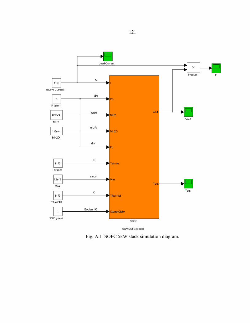
121

Fig. A.1 SOFC 5kW stack simulation diagram.

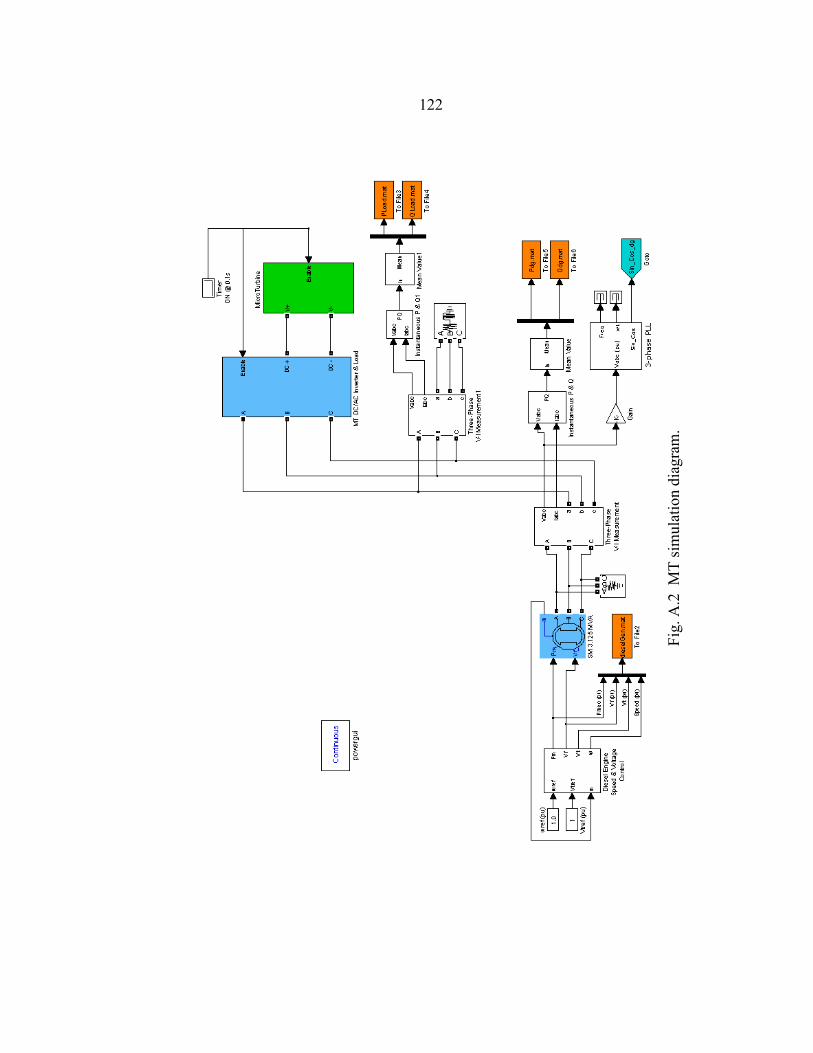
122

Fig.

A.2

MT

sim

ulat

ion

diag

ram

.

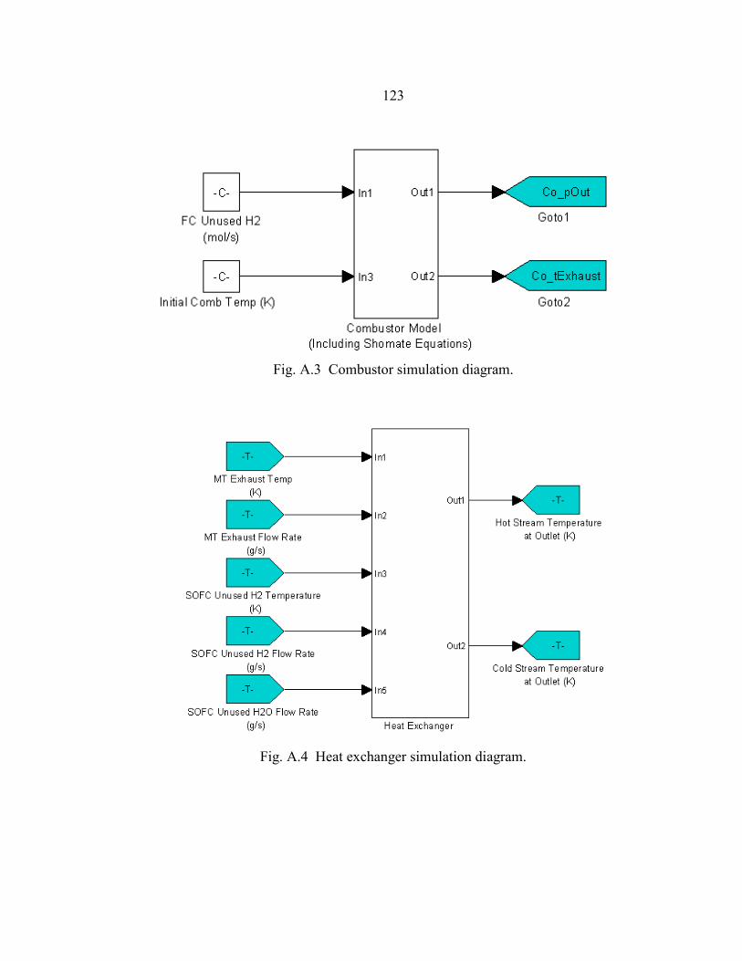
123

Fig. A.3 Combustor simulation diagram.

Fig. A.4 Heat exchanger simulation diagram.