Embed Size (px)
Citation preview
Investigation on the Drag Coe�cient of the Steadyand Unsteady Flow Conditions in Coarse PorousMediaHadi Norouzi ( [email protected] )
University of Zanjan https://orcid.org/0000-0001-6082-3736Jalal Bazargan
University of ZanjanFaezah Azhang
University of ZanjanRana Nasiri
University of Zanjan
Research Article
Keywords: Drag Coe�cient, Friction Coe�cient, Hydraulic Gradient, Porous Media, Steady and UnsteadyFlow
Posted Date: March 24th, 2021
DOI: https://doi.org/10.21203/rs.3.rs-332975/v1
License: This work is licensed under a Creative Commons Attribution 4.0 International License. Read Full License
1
Investigation on the Drag Coefficient of the Steady and Unsteady Flow Conditions in 1
Coarse Porous Media 2
d, Rana Nasiric, Faezeh Azhangb, Jalal Bazargan a* Hadi Norouzi 3
a. PhD Candidate of Hydraulic Structures, Department of Civil Engineering, University of 4
)[email protected], Zanjan, Iran ( 5
b. Associate Professor, Department of Civil Engineering, University of Zanjan, Zanjan, Iran 6
) [email protected]( 7
c. Masters of Hydraulic Structures, Department of Civil Engineering, University of Zanjan, 8
)[email protected], Iran ( 9
d. Masters of Hydraulic Structures, Department of Civil Engineering, University of Zanjan, 10
)[email protected], Iran ( 11
Abstract 12
The study of the steady and unsteady flow through porous media and the interactions between 13
fluids and particles is of utmost importance. In the present study, binomial and trinomial 14
equations to calculate the changes in hydraulic gradient (i) in terms of flow velocity (V) were 15
studied in the steady and unsteady flow conditions, respectively. According to previous 16
studies, the calculation of drag coefficient (Cd) and consequently, drag force (Fd) is a function 17
of coefficient of friction (f). Using Darcy-Weisbach equations in pipes, the hydraulic gradient 18
equations in terms of flow velocity in the steady and unsteady flow conditions, and the 19
analytical equations proposed by Ahmed and Sunada in calculation of the coefficients a and b 20
of the binomial equation and the friction coefficient (f) equation in terms of the Reynolds 21
number (Re) in the porous media, equations were presented for calculation of the friction 22
coefficient in terms of the Reynolds number in the steady and unsteady flow conditions in 1D 23
2
(one-dimensional) confined porous media. Comparison of experimental results with the 24
results of the proposed equation in estimation of the drag coefficient in the present study 25
confirmed the high accuracy and efficiency of the equations. The mean relative error (MRE) 26
between the computational (using the proposed equations in the present study) and 27
observational (direct use of experimental data) friction coefficient for small, medium and 28
large grading in the steady flow conditions was equal to 1.913, 3.614 and 3.322%, 29
respectively. In the unsteady flow condition, the corresponding values of 7.806, 14.106 and 30
10.506 % were obtained, respectively. 31
Keywords: Drag Coefficient, Friction Coefficient, Hydraulic Gradient, Porous Media, 32
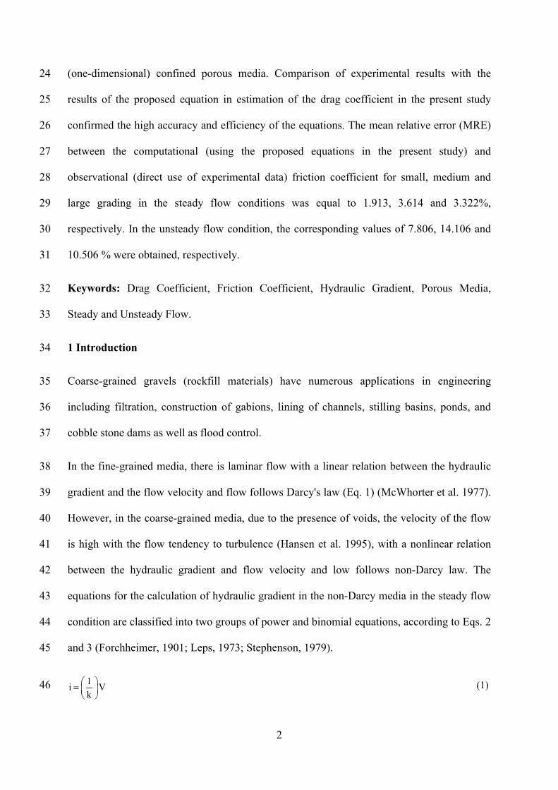
Steady and Unsteady Flow. 33
1 Introduction 34
Coarse-grained gravels (rockfill materials) have numerous applications in engineering 35
including filtration, construction of gabions, lining of channels, stilling basins, ponds, and 36
cobble stone dams as well as flood control. 37
In the fine-grained media, there is laminar flow with a linear relation between the hydraulic 38
gradient and the flow velocity and flow follows Darcy's law (Eq. 1) (McWhorter et al. 1977). 39
However, in the coarse-grained media, due to the presence of voids, the velocity of the flow 40
is high with the flow tendency to turbulence (Hansen et al. 1995), with a nonlinear relation 41
between the hydraulic gradient and flow velocity and low follows non-Darcy law. The 42
equations for the calculation of hydraulic gradient in the non-Darcy media in the steady flow 43
condition are classified into two groups of power and binomial equations, according to Eqs. 2 44
and 3 (Forchheimer, 1901; Leps, 1973; Stephenson, 1979). 45
1i V
k
=
(1) 46
3
nmVi = (2) 47
2bVaVi += (3) 48
The binomial equation was proved by dimensional analysis by Ward (1964) and by the 49
Navier-Stokes equations by Ahmed and Sunada (1969) and has a higher accuracy and 50
efficiency in comparison to the exponential equation (Stephenson 1979, Leps 1973). 51
Ergun (1952) studied the coefficients of the binomial equation of the hydraulic gradient by 52
passing nitrogen gas through a cylinder with an area of 7.24 cm2 that was filled with 53
aggregate and presented Eq. (4) to calculate the coefficients a, b. 54
( )32
21
150gnd
na
−=
υ ,
( )3
175.1gdn
nb
−= (4) 55
Ward (1964) presented Eq. (5), which can be proved using dimensional analysis, to calculate 56
the coefficients a and b in the free surface porous media. 57
gka
υ= ,
kg
Cb W
′= (5) 58
Kovacs (1980) studied a set of data with a Reynolds number range of 10 to 100 (according to 59
his definition of the Reynolds number) and presented an equation similar to that of Ergun 60
(Eq. (6)). 61
( )23
21144
dgn
na
−=
ν ,
( )dgn
nb
3
14.2 −= (6) 62
Ahmed and Sunada (1969) presented Eq. (7) to calculate the coefficients a and b using the 63
Navier-Stokes equations. 64
gka
ρµ
= , ckg
b1
= ,(7) 2CdK = 65
4
Ergun-Reichelt presented an equation for calculation of the coefficients a, b (Eq. (8)) (Fand 66
and Thinakaran, 1990). 67
( )23
22 1214
dgn
nMa
ν−= ,
( )dgn
nMb
3
157.1
−= , ( )nD
dM
−+=
13
21 (8) 68
Equations (4) to (8) and several equations including those proposed by (Muskrat 1937; 69
Engelund 1953; Irmay 1958; Stephenson 1979; Jent 1991; Kadlec and Knight 1996; 70
Sidiropoulou et al. 2007; Sedghi and Rahimi 2011) were presented to calculate the 71
coefficients of the binomial equation (a, b) in steady flow conditions. A semi-analytical 72
solution of the nonlinear differential equations constructing a fully saturated porous medium 73
is presented by (Abbas et al. 2021). 74
A comprehensive equation with respect to the effects of unsteady flow conditions was 75
proposed by Polubarinova-Kochino (1952) (Eq. (9)) (Hannoura and McCorcoudale, 1985). 76
++=dt
dVcbVaVi 2 (9) 77
Where the coefficient of the third term (c) is obtained using Eq. (10). 78
( )ng
nCnc m −+
=1
(10) 79
Where Cm represents the proportion of fluid that vibrates with the vibration of the particle. In 80
other words, Cm is the added mass coefficient. 81
Hannoura and McCorquodale (1985) performed an experimental study and indicated that Cm 82
was insignificant and negligible. In other words, by removing Cm from Eq. (10), the third 83
term of Eq. (9) can be expressed as Eq. (11). 84
=
dt
dV
gdt
dVc
1 (11) 85
5
where V is flow velocity (m/s), k is hydraulic conductivity (s/m), i is hydraulic gradient, m 86
and n are values dependent on the properties of the porous media, fluid and flow, while a and 87
b are coefficients that are dependent on the properties of the porous media as well as the 88
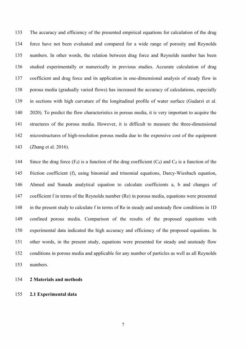
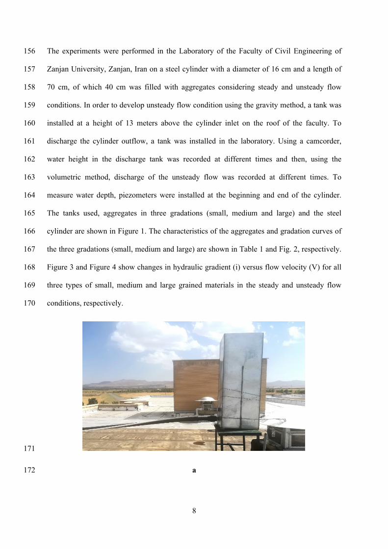
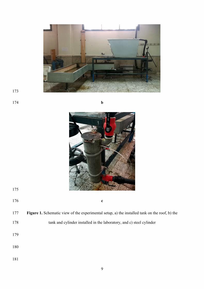
fluid. 89
Shokri et al. (2011) experimentally studied unsteady flow in a free surface coarse-grained 90
porous media and concluded that the third term (
dt
dVc ) has insignificant effect on the 91
accuracy of calculations. 92
In the present study, the binomial (Eq. 3) and trinomial (Eq. 8) equations were used to 93
calculate the changes in hydraulic gradient in terms of velocity in steady and unsteady flow 94
conditions, respectively. 95
The simulated annealing algorithm is often used for water resources management, model 96
calibration, decision making, etc. (Bechler et al. 2013; Cao and Ye 2013; Jiang et al. 2018). 97
(Hu et al. 2019) Kriging-approximation simulated annealing (KASA) optimization algorithm 98
has been used to optimize the flow parameters in the porous media. 99
Particle swarm optimization (PSO) algorithm is a population-based evolutionary algorithm 100
and is used in civil engineering and water resources optimization problems such as reservoir 101
performance (Nagesh Kumar and Janga Reddy, 2007), water quality management (Afshar et 102
al. 2011, Lu et al. 2002, Chau, 2005) and optimization of the Muskingum method coefficients 103
(Chu and Chang 2009, Moghaddam et al. 2016, Bazargan and Norouzi 2018, Norouzi and 104
Bazargan 2020, Norouzi and Bazargan 2021). Therefore, in the present study, the particle 105
swarm optimization (PSO) algorithm was used to optimize the coefficients of the 106
Forchheimer binomial equation (Eq. 3) as well as the Polubarinova-Kochino trinomial 107
equation (Eq. 8). 108
6
In addition to the above classification, flow in the coarse-grained media can be classified into 109
the following two general groups. 110
A: Free surface flow through and on coarse-grained layers such as gabions and gravel dams 111
in which the flow is in contact with the free environment on one side. 112
B: Confined flow through coarse-grained layers such as coarse-grained filters of rockfill 113
dams and coarse-grained layers confined between concrete elements and fine materials of 114
hydraulic structures. In such layers, flow from all sides is in contact with an impermeable 115
layer or a layer with low permeability in comparison to gravel materials. 116
The study of flow through confined porous media is of great importance in geology (Lei et al. 117
2017), petroleum (Song et al. 2014) and industry (Rahimi et al. 2017). Flow through 118
pressurized porous media has been studied experimentally and numerically by (Ingham and 119
Pop 2005; Sheikh and Pak 2015; and Zhu et al. 2016). The study of fluid flow in porous 120
media is performed by a network of capillary pipes with a microscopic approach by (Hoang 121
et al. 2013). (Hsu and Chen 2010) proposes a multiscale flow and transport model in three-122
dimensional fractal random fields for use in porous media. 123
Estimation of drag force due to flow-aggregate interactions is very important in modeling of 124
confined porous media (Sheikh and Qiu, 2018). Pore-scale drag and relative motion between 125
fluid and aggregates are important due to the formation of non-uniform velocity and 126
consequently, the formation of non-uniform force (Sheikh and Qiu, 2018). (Ergun 1952; Wen 127
and Yu 1966; Di Felice 1994; Schlichting and Gersten 2000; Hill et al. 2001a; Hill et al. 128
2001b; Van der Hoef et al. 2005; Bird et al. 2007; Yin and Sundaresan 2009; Zhang et al. 129
2011; Rong et al. 2013) studied the drag force in the confined porous media considering a 130
certain number of particles. The flow regime and drag force of a single particle are different 131
from those of interactive particles (Zhu et al. 1994; Liang et al. 1996; Chen and Wu 2000). 132
7
The accuracy and efficiency of the presented empirical equations for calculation of the drag 133
force have not been evaluated and compared for a wide range of porosity and Reynolds 134
numbers. In other words, the relation between drag force and Reynolds number has been 135
studied experimentally or numerically in previous studies. Accurate calculation of drag 136
coefficient and drag force and its application in one-dimensional analysis of steady flow in 137
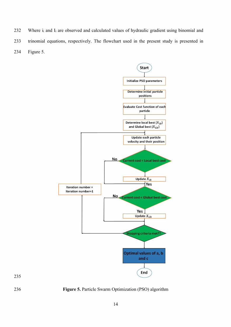
porous media (gradually varied flows) has increased the accuracy of calculations, especially 138
in sections with high curvature of the longitudinal profile of water surface (Gudarzi et al. 139
2020). To predict the flow characteristics in porous media, it is very important to acquire the 140
structures of the porous media. However, it is difficult to measure the three-dimensional 141
microstructures of high-resolution porous media due to the expensive cost of the equipment 142
(Zhang et al. 2016). 143
Since the drag force (Fd) is a function of the drag coefficient (Cd) and Cd is a function of the 144
friction coefficient (f), using binomial and trinomial equations, Darcy-Wiesbach equation, 145
Ahmed and Sunada analytical equation to calculate coefficients a, b and changes of 146
coefficient f in terms of the Reynolds number (Re) in porous media, equations were presented 147
in the present study to calculate f in terms of Re in steady and unsteady flow conditions in 1D 148
confined porous media. Comparison of the results of the proposed equations with 149
experimental data indicated the high accuracy and efficiency of the proposed equations. In 150
other words, in the present study, equations were presented for steady and unsteady flow 151
conditions in porous media and applicable for any number of particles as well as all Reynolds 152
numbers. 153
2 Materials and methods 154
2.1 Experimental data 155
8
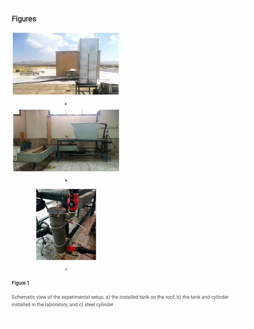
The experiments were performed in the Laboratory of the Faculty of Civil Engineering of 156
Zanjan University, Zanjan, Iran on a steel cylinder with a diameter of 16 cm and a length of 157
70 cm, of which 40 cm was filled with aggregates considering steady and unsteady flow 158
conditions. In order to develop unsteady flow condition using the gravity method, a tank was 159
installed at a height of 13 meters above the cylinder inlet on the roof of the faculty. To 160
discharge the cylinder outflow, a tank was installed in the laboratory. Using a camcorder, 161
water height in the discharge tank was recorded at different times and then, using the 162
volumetric method, discharge of the unsteady flow was recorded at different times. To 163
measure water depth, piezometers were installed at the beginning and end of the cylinder. 164
The tanks used, aggregates in three gradations (small, medium and large) and the steel 165
cylinder are shown in Figure 1. The characteristics of the aggregates and gradation curves of 166
the three gradations (small, medium and large) are shown in Table 1 and Fig. 2, respectively. 167
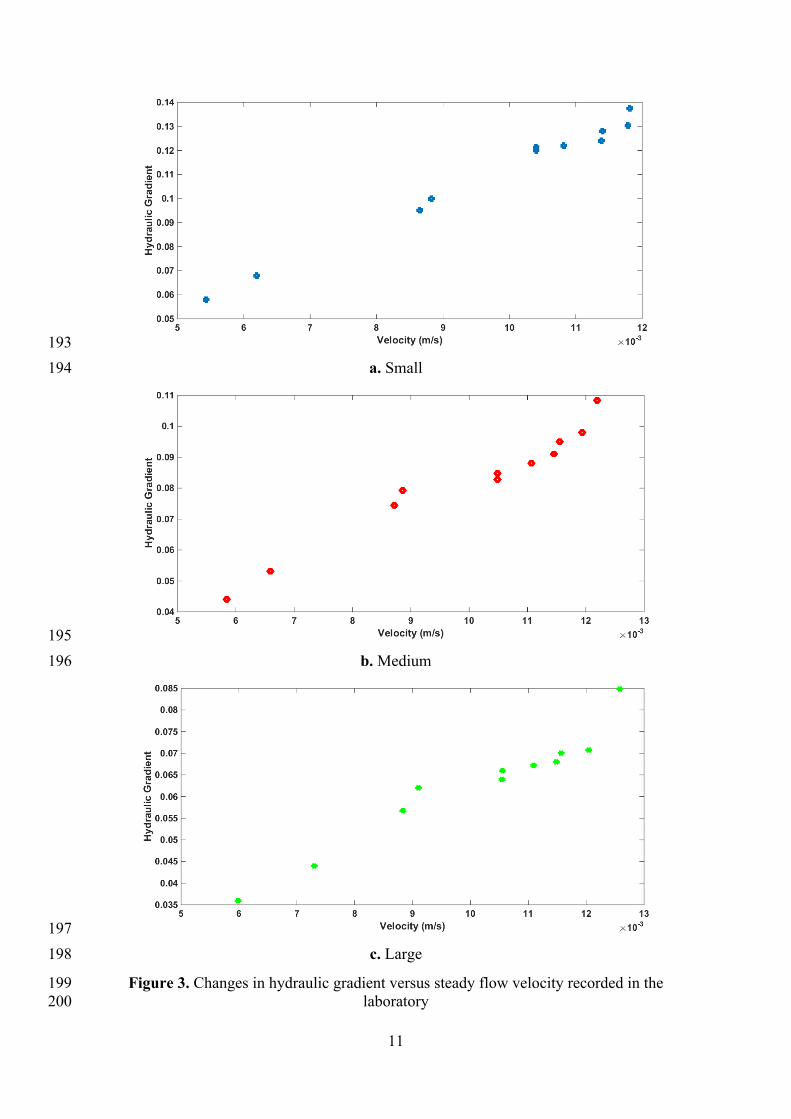
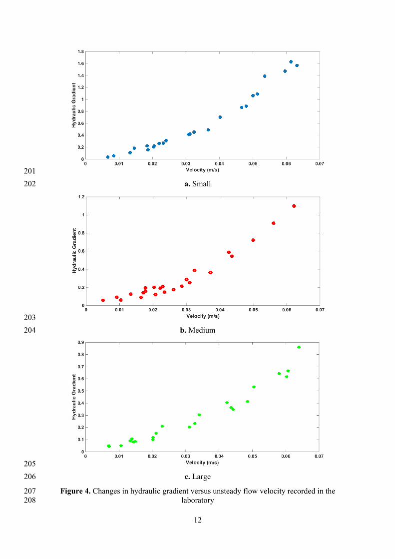
Figure 3 and Figure 4 show changes in hydraulic gradient (i) versus flow velocity (V) for all 168
three types of small, medium and large grained materials in the steady and unsteady flow 169
conditions, respectively. 170
171
a 172
9
173
b 174
175
c 176
Figure 1. Schematic view of the experimental setup, a) the installed tank on the roof, b) the 177
tank and cylinder installed in the laboratory, and c) steel cylinder 178
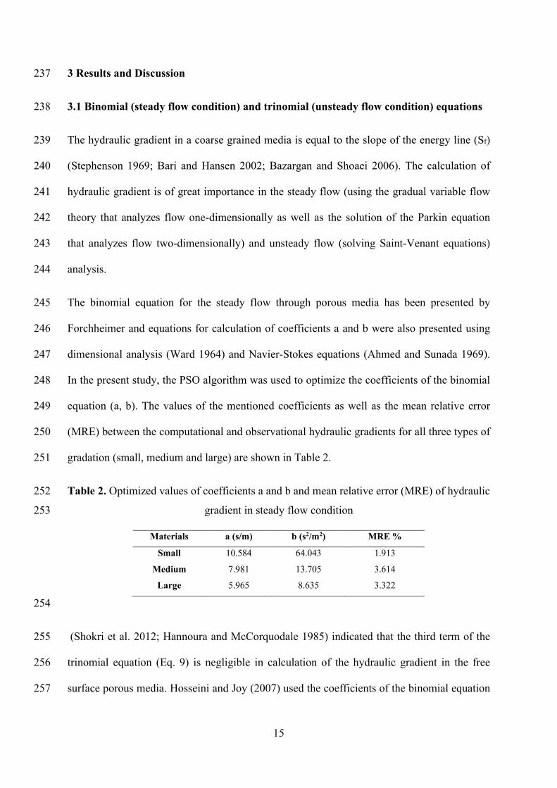
179
180
181
10
Table 1. Characteristics of the experimental materials 182
Materials 0 d
(mm)
10d
(mm)
30d
(mm)
50d
(mm)
60d
(mm)
100d
(mm)
Cu Cc porosity
Small 4 7 10 12.5 14.5 22 1.69 0.69 0358
Medium 4.75 14.5 18.5 19 21.3 32 1.16 0.95 0.410
Large 12.7 22.7 23.9 22 25.05 32 1.11 0.99 0.448
183
In Table 1, the coefficient of uniformity (Cu) and the coefficient of curvature (Cc) were equal 184
to 10
60
D
Dand
( )6010
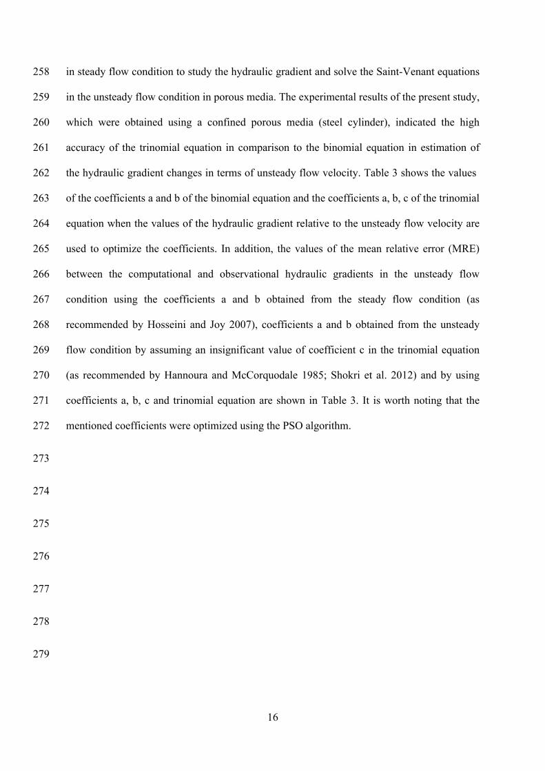
2
30
*DD
D, respectively. 185
186
Figure 2. Gradation curve of different materials 187
188
189
190
191
192
11
193
a. Small 194
195
b. Medium 196
197
c. Large 198
Figure 3. Changes in hydraulic gradient versus steady flow velocity recorded in the 199
laboratory 200
12
201
a. Small 202
203
b. Medium 204
205
c. Large 206
Figure 4. Changes in hydraulic gradient versus unsteady flow velocity recorded in the 207
laboratory 208
13
2.2 Particle Swarm Optimization (PSO) Algorithm 209
PSO method is also a population based evolutionary search optimization method inspired 210
from the movement of bird flock (swarm) (Eberhart and Kennedy 1995; Chau 2007; Clerc 211
and Kennedy 2002). The basic idea in PSO is based on the assumption that potential solutions 212
are flown through hyperspace with acceleration towards more optimum solutions. Each 213
particle adjusts its flying according to the experiences of both itself and its companions. 214
During the process; the overall best value attained by all the particles within the group and 215
the coordinates of each element in hyperspace associated with its previous best fitness 216
solution are recorded in the memory (Chau 2007; Kumar and Reddy 2007). The details of 217
PSO can be obtained elsewhere (Shi and Eberhart 1998; Clerc and Kennedy 2002; Chau 218
2007; Gurarslan and Karahan 2011; Karahan 2012; Di Cesare et al. 2015). Various 219
algorithms have been used to optimize the parameters of the Forchheimer equation and other 220
methods and other issues that need to be optimized, one of the fastest, most acceptable and 221
most widely used is the PSO algorithm, which has been confirmed by previous researchers. 222
since in previous studies, efficiency, high convergence speed and proper accuracy of the PSO 223
algorithm have been examined and approved, therefore, among different algorithms, the PSO 224
algorithm is selected to optimize the Forchheimer equation coefficients (a, b) and 225
Polubarinova-Kochino equation coefficient (a, b, c). 226
To evaluate the optimum values of the binomial equation coefficients (a, b) and the trinomial 227
equation coefficients (a, b, c), the minimization of the Mean Relative Error (MRE), which is 228
defined using Eq. (12), was used as the objective function in the Particle Swarm Optimization 229
algorithm. 230
∑=
−=
n
i i
ii
i
Ii
nMRE
1
100*1 (12) 231
14
Where ii and Ii are observed and calculated values of hydraulic gradient using binomial and 232
trinomial equations, respectively. The flowchart used in the present study is presented in 233
Figure 5. 234
235
Figure 5. Particle Swarm Optimization (PSO) algorithm 236
15
3 Results and Discussion 237
3.1 Binomial (steady flow condition) and trinomial (unsteady flow condition) equations 238
The hydraulic gradient in a coarse grained media is equal to the slope of the energy line (Sf) 239
(Stephenson 1969; Bari and Hansen 2002; Bazargan and Shoaei 2006). The calculation of 240
hydraulic gradient is of great importance in the steady flow (using the gradual variable flow 241
theory that analyzes flow one-dimensionally as well as the solution of the Parkin equation 242
that analyzes flow two-dimensionally) and unsteady flow (solving Saint-Venant equations) 243
analysis. 244
The binomial equation for the steady flow through porous media has been presented by 245
Forchheimer and equations for calculation of coefficients a and b were also presented using 246
dimensional analysis (Ward 1964) and Navier-Stokes equations (Ahmed and Sunada 1969). 247
In the present study, the PSO algorithm was used to optimize the coefficients of the binomial 248
equation (a, b). The values of the mentioned coefficients as well as the mean relative error 249
(MRE) between the computational and observational hydraulic gradients for all three types of 250
gradation (small, medium and large) are shown in Table 2. 251
Table 2. Optimized values of coefficients a and b and mean relative error (MRE) of hydraulic 252
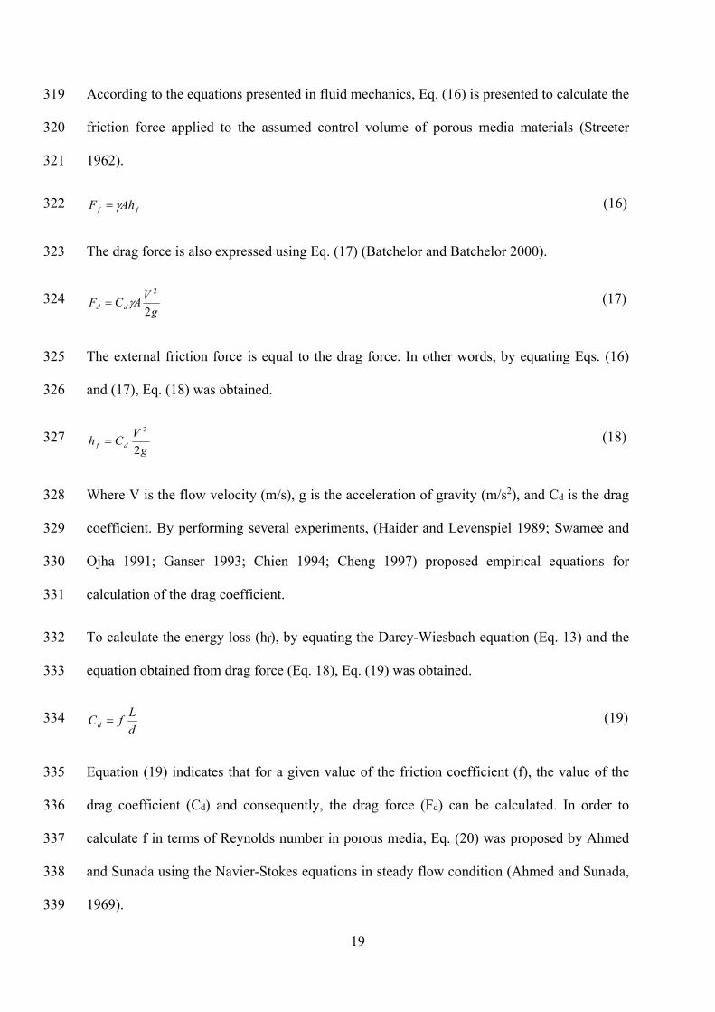
gradient in steady flow condition 253
Materials a (s/m) b (s2/m2) MRE %
Small 10.584 64.043 1.913
Medium 7.981 13.705 3.614
Large 5.965 8.635 3.322
254
(Shokri et al. 2012; Hannoura and McCorquodale 1985) indicated that the third term of the 255
trinomial equation (Eq. 9) is negligible in calculation of the hydraulic gradient in the free 256
surface porous media. Hosseini and Joy (2007) used the coefficients of the binomial equation 257
16
in steady flow condition to study the hydraulic gradient and solve the Saint-Venant equations 258
in the unsteady flow condition in porous media. The experimental results of the present study, 259
which were obtained using a confined porous media (steel cylinder), indicated the high 260
accuracy of the trinomial equation in comparison to the binomial equation in estimation of 261
the hydraulic gradient changes in terms of unsteady flow velocity. Table 3 shows the values 262
of the coefficients a and b of the binomial equation and the coefficients a, b, c of the trinomial 263
equation when the values of the hydraulic gradient relative to the unsteady flow velocity are 264
used to optimize the coefficients. In addition, the values of the mean relative error (MRE) 265
between the computational and observational hydraulic gradients in the unsteady flow 266
condition using the coefficients a and b obtained from the steady flow condition (as 267
recommended by Hosseini and Joy 2007), coefficients a and b obtained from the unsteady 268
flow condition by assuming an insignificant value of coefficient c in the trinomial equation 269
(as recommended by Hannoura and McCorquodale 1985; Shokri et al. 2012) and by using 270
coefficients a, b, c and trinomial equation are shown in Table 3. It is worth noting that the 271
mentioned coefficients were optimized using the PSO algorithm. 272
273
274
275
276
277
278
279
17
Table 3. Values of the optimized coefficients a and b using steady and unsteady flow data 280
and coefficients a, b, c of unsteady flow data and mean relative error (MRE) values of 281
hydraulic gradient of unsteady flow 282
Regime Equations Coefficients Small Medium Large
Steady
a (s/m) 10.584 7.91 5.965
Binomial b (s2/m2) 64.043 13.705 8.635
MRE % 25.567 25.923 21.306
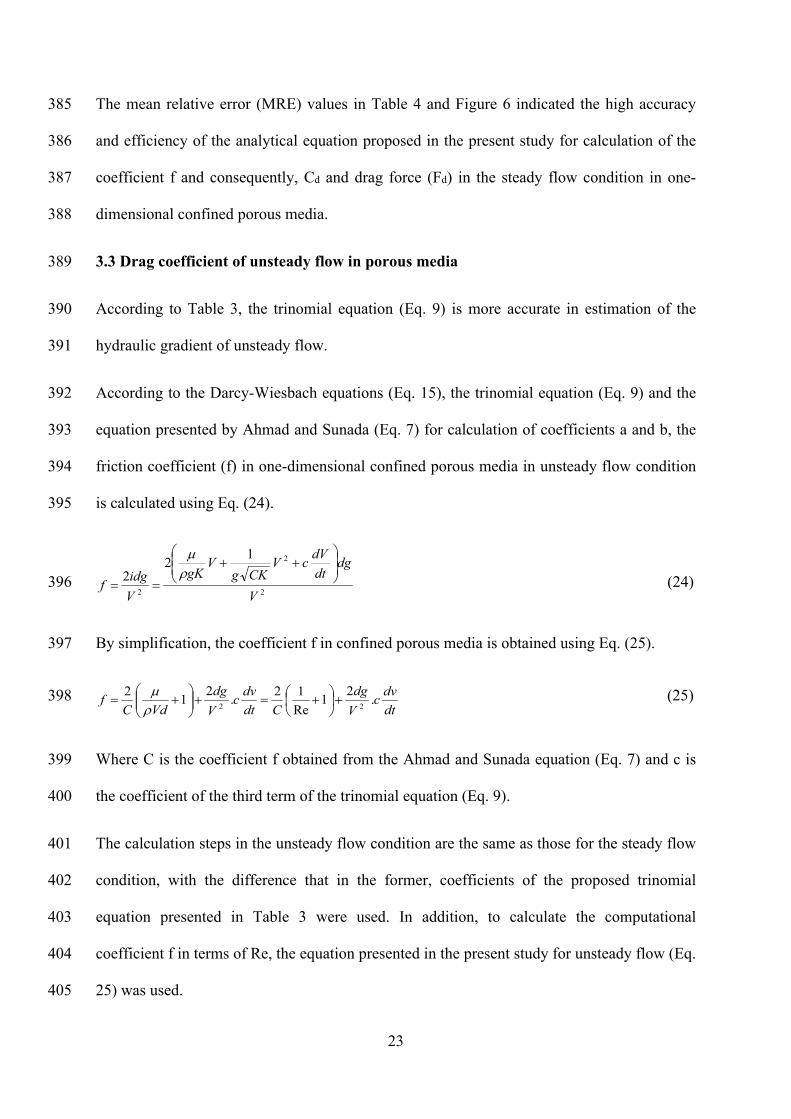
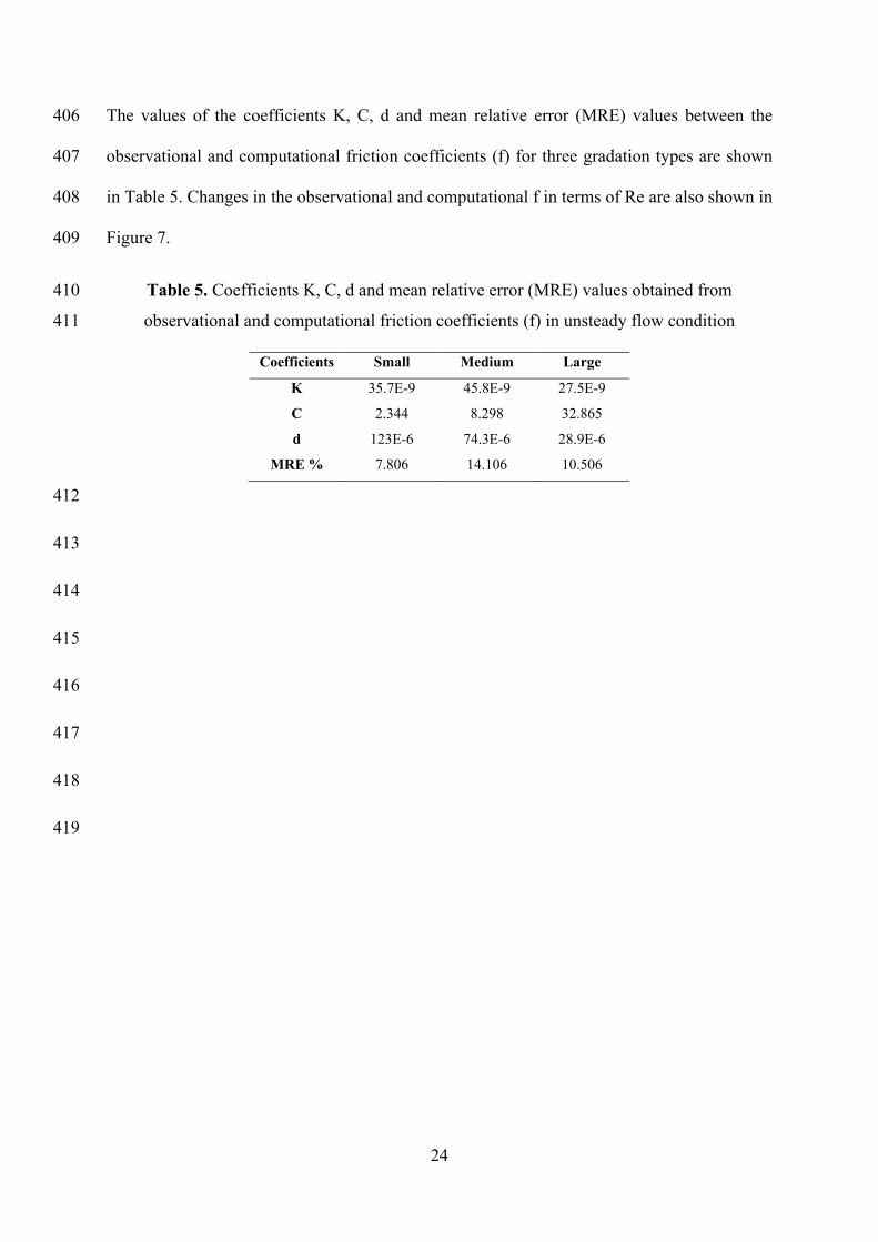
Unsteady
a (s/m) 3.848 5.255 5.411
Binomial b (s2/m2) 331.714 165.084 80.344
MRE % 10.024 22.599 12.941
Unsteady
a (s/m) 2.859 2.225 3.704
Trinomial b (s2/m2) 352.622 165.336 107.186
c (s2/m) 10.369 51.369 14.581
MRE % 7.806 14.106 10.506
283
As can be seen from Table 3, if the coefficients a and b obtained from the steady flow 284
condition were used to calculate the changes in the hydraulic gradient relative to the unsteady 285
flow velocity, the mean relative error (MRE) values of 25.567, 25.923, and 21.306 were 286
obtained for the small, medium and large grained materials, respectively. In the case of using 287
the coefficients a and b obtained from the unsteady flow data, the corresponding MRE values 288
of 10.024, 22.599 and 12.941%, were obtained, respectively. In addition, by using the 289
optimized coefficients a, b, and c of the trinomial equation, the corresponding MRE values of 290
7.806, 14.106 and 10.506% were obtained, respectively. The MRE values of the trinomial 291
equation in comparison to those of the binomial equation in case of using the coefficients a 292
and b obtained from the unsteady flow condition for three gradation types improved by 22, 38 293
and 19%, respectively. The corresponding values in case of using the coefficients a and b 294
obtained from the steady flow condition improved by 70, 46 and 51%, respectively. In other 295
words, in order to calculate the hydraulic gradient in the unsteady flow condition, the use of 296
the coefficients a, b, and c of the unsteady flow and the trinomial equation, coefficients a and 297
18
b obtained from the unsteady flow data, and coefficients a and b obtained from the steady 298
flow data were more accurate, respectively. 299
3.2 Drag coefficient in porous media 300
In addition to power equations (Eq. 2) and Forchheimer binomial equation (Eq. 3), one of the 301
methods of flow analysis in porous media is the use of friction coefficient (f) in terms of 302
Reynolds number (Re). Accordingly, the flow energy loss in porous media is obtained using 303
an equation similar to the Darcy-Weisbach equation (Stephenson 1979; Herrera and Felton 304
1991). For the confined flow in the pipes, the Darcy-Wiesbach equation is expressed using 305
Eq. (13). 306
g
V
d
Lfh f
2.
2
= (13) 307
Where f is the (dimensionless) friction coefficient, L is the pipe length (m), d is the pipe 308
diameter (m), V is flow velocity (m/s), g is the acceleration of gravity (m/s2), and hf is the 309
energy loss (m). 310
Since hf/L is equal to the hydraulic gradient, Eq. (13) can be rewritten as Eq. (14). 311
g
V
d
fi
2.
2
= (14) 312
Leps (1973) indicated the velocity corresponding head in the above equations asmg
V 2
, with m 313
value of 2 according to the Darcy-Wiesbach equation in pipes. Stephenson (1979) assumed 314
the formation of the porous media inside a set of winding tubes within a set of aggregates 315
with pores, considered the value of m in the energy loss (hf) equation equal to 1 and proposed 316
Eq. (15) to calculate the hydraulic gradient. 317
g
V
d
fi
2
.= (15) 318
19
According to the equations presented in fluid mechanics, Eq. (16) is presented to calculate the 319
friction force applied to the assumed control volume of porous media materials (Streeter 320
1962). 321
ff AhF γ= (16) 322
The drag force is also expressed using Eq. (17) (Batchelor and Batchelor 2000). 323
g
VACF dd
2
2
γ= (17) 324
The external friction force is equal to the drag force. In other words, by equating Eqs. (16) 325
and (17), Eq. (18) was obtained. 326
g
VCh df
2
2
= (18) 327
Where V is the flow velocity (m/s), g is the acceleration of gravity (m/s2), and Cd is the drag 328
coefficient. By performing several experiments, (Haider and Levenspiel 1989; Swamee and 329
Ojha 1991; Ganser 1993; Chien 1994; Cheng 1997) proposed empirical equations for 330
calculation of the drag coefficient. 331
To calculate the energy loss (hf), by equating the Darcy-Wiesbach equation (Eq. 13) and the 332
equation obtained from drag force (Eq. 18), Eq. (19) was obtained. 333
d
LfCd = (19) 334
Equation (19) indicates that for a given value of the friction coefficient (f), the value of the 335
drag coefficient (Cd) and consequently, the drag force (Fd) can be calculated. In order to 336
calculate f in terms of Reynolds number in porous media, Eq. (20) was proposed by Ahmed 337
and Sunada using the Navier-Stokes equations in steady flow condition (Ahmed and Sunada, 338
1969). 339
20
1Re
1+=f ,
µρVd
=Re (20) 340
Where ρ is water density (1000 kg/m3) and µ is water viscosity (0.001 kg/m.s). According 341
to Eqs. (19) and (20), the drag coefficient in the free surface porous media is calculated using 342
Eq. (21). 343
d
LCd
+= 1
Re
1 (21) 344
Where d is calculated using the equations proposed by Ahmed and Sunada (1969) 345
(Eq. 7, K = cd2). 346
Results of the present study showed that the friction coefficient (f) in one-dimensional 347
confined porous media in the steady and unsteady flow conditions is different from Eq. (20). 348
3.3 Drag coefficient of steady flow in porous media 349
According to Darcy-Wiesbach equations (Eq. 15), the binomial equation (Eq. 3), and the 350
equation of coefficients a and b presented by Ahmed and Sunada (Eq. 7), the friction 351
coefficient (f) in one-dimensional confined porous media in the steady flow condition is 352
calculated using Eq. (22). 353
2
2
2
12
2
V
dgVCKg
VgK
V
idgf
+
==ρ
µ
(22) 354
With simplification, Eq. (24) can be written as Eq. (23). 355
+=
+= 1
Re
121
2
CVdCf
ρµ (23) 356
In other words, in the steady flow condition in one-dimensional confined porous media, the 357
friction coefficient (f) is 2/C times the friction coefficient (f) in the free surface porous media. 358
21
The present study considering the steady flow condition in one-dimensional confined porous 359
media included the following steps: 360
1) Using experimental data, hydraulic gradient (i) (Fig. 4) in terms of flow velocity (V), the 361
optimized coefficients a and b using the PSO algorithm (Table 2), coefficients K, C and d 362
using Eq. (7) were calculated for small, medium and large-grained particles and summarized 363
in Table (4). 364
2) The friction coefficient (f) using Eq. (15), which is the same as the observational friction 365
coefficient, Reynolds number (Re) using Eq. (20), computational friction coefficient (f) using 366
the presented equation in the present study (Eq. 23) was calculated for the three gradations. 367
Figure 6 shows the changes in the friction coefficient (f) versus Reynolds number of steady 368
flow. 369
3) Observational friction coefficient (calculated directly from experimental data and Eq. (15)) 370
was compared with computational friction coefficient (calculated using Eq. (23), which was 371
presented in the present study for steady flow condition) and mean relative error (MRE) 372
values are shown in Table 4. 373
Table 4. Coefficients K, C, d and mean relative error (MRE) values obtained from 374
observational and computational friction coefficients (f) in steady flow condition 375
Coefficients Small Medium Large
K 9.6E-9 12.8E-9 17.1E-9
C 263.041 4331.704 8154.079
d 6.051E-6 1.717E-6 1.448E-6
MRE % 1.913 3.614 3.322
376
22
377
a. Small 378
379
b. Medium 380
381
c. Large 382
Figure 6. Observational and computational friction coefficient versus Reynolds number in 383
steady flow condition 384
23
The mean relative error (MRE) values in Table 4 and Figure 6 indicated the high accuracy 385
and efficiency of the analytical equation proposed in the present study for calculation of the 386
coefficient f and consequently, Cd and drag force (Fd) in the steady flow condition in one-387
dimensional confined porous media. 388
3.3 Drag coefficient of unsteady flow in porous media 389
According to Table 3, the trinomial equation (Eq. 9) is more accurate in estimation of the 390
hydraulic gradient of unsteady flow. 391
According to the Darcy-Wiesbach equations (Eq. 15), the trinomial equation (Eq. 9) and the 392
equation presented by Ahmad and Sunada (Eq. 7) for calculation of coefficients a and b, the 393
friction coefficient (f) in one-dimensional confined porous media in unsteady flow condition 394
is calculated using Eq. (24). 395
2
2
2
12
2
V
dgdt
dVcV
CKgV
gK
V
idgf
++
==ρ
µ
(24) 396
By simplification, the coefficient f in confined porous media is obtained using Eq. (25). 397
dt
dvc
V
dg
Cdt
dvc
V
dg
VdCf .
21
Re
12.
21
222
+
+=+
+=
ρµ (25) 398
Where C is the coefficient f obtained from the Ahmad and Sunada equation (Eq. 7) and c is 399
the coefficient of the third term of the trinomial equation (Eq. 9). 400
The calculation steps in the unsteady flow condition are the same as those for the steady flow 401
condition, with the difference that in the former, coefficients of the proposed trinomial 402
equation presented in Table 3 were used. In addition, to calculate the computational 403
coefficient f in terms of Re, the equation presented in the present study for unsteady flow (Eq. 404
25) was used. 405
24
The values of the coefficients K, C, d and mean relative error (MRE) values between the 406
observational and computational friction coefficients (f) for three gradation types are shown 407
in Table 5. Changes in the observational and computational f in terms of Re are also shown in 408
Figure 7. 409
Table 5. Coefficients K, C, d and mean relative error (MRE) values obtained from 410
observational and computational friction coefficients (f) in unsteady flow condition 411
Coefficients Small Medium Large
K 35.7E-9 45.8E-9 27.5E-9
C 2.344 8.298 32.865
d 123E-6 74.3E-6 28.9E-6
MRE % 7.806 14.106 10.506
412
413
414
415
416
417
418
419
25
420
a. Small 421
422
b. Medium 423
424
c. Large 425
Figure 7. Changes in observational and computational friction coefficients in terms of 426
Reynolds number in unsteady flow condition 427
26
The mean relative error (MRE) values (Table 5) as well as the changes in the observational 428
and computational f values in terms of Re (Fig. 6) indicated the high accuracy and efficiency 429
of the proposed equation in the present study to calculate f and consequently, Cd and Fd for 430
unsteady flow in one-dimensional confined porous media. 431
4 Conclusions 432
In the present study, steady and unsteady flows in one-dimensional confined porous media 433
were studied to calculate the changes in hydraulic gradient (i) in terms of flow velocity (V) 434
and drag force (Fd) considering small, medium and large grained materials. The calculation of 435
drag coefficient (Cd) is the most important step in calculations of Fd. On the other hand, 436
according to performed studies, the only important parameter in calculation of the Cd in a 437
porous media is the friction coefficient (f). For this reason, in the present study, to calculate 438
the coefficient f in terms of Reynolds number (Re), the Darcy-Wiesbach equation in pipes, 439
the equations of i in terms of V (in the steady flow condition as a binomial equation and in 440
the unsteady flow condition as a trinomial equation), and the analytical equation by Ahmad 441
and Sunada in calculation of the coefficients a, b and coefficient f in terms of Re in porous 442
media, an equation for steady flow condition and another equation for unsteady flow 443
condition in one-dimensional confined porous media were presented, which have many 444
applications in civil engineering, mechanics, geology, and oil industry. The proposed 445
equations for the f coefficient in terms of Re in both steady and unsteady flow conditions 446
were evaluated using experimental data and the results showed the accuracy and efficiency of 447
these equations in estimation of the coefficient f and consequently, Cd and Fd. In general, the 448
results of the present study include the followings. 449
1) Comparison of the accuracy of the hydraulic gradient calculations in terms of flow velocity 450
in unsteady flow conditions with the methods of a) trinomial equation, b) binomial equation 451
27
and coefficients a and b obtained from unsteady flow data by assuming an insignificant 452
coefficient c, and C) binomial equation and coefficients a and b obtained from steady flow 453
data showed that the methods a to c are more accurate, respectively. 454
2) Mean relative error (MRE) values between observational coefficients f in the steady flow 455
condition (direct use of experimental data to calculate coefficient f) and computational f 456
coefficients (using the proposed equation in the present study to calculate coefficient f in the 457
steady flow condition) for small, medium and large grained materials were equal to 1.913, 458
3.614 and 3.322%, respectively. 459
3) By using the proposed equation in the present study to calculate the coefficient f in 460
unsteady flow condition and then, comparing the computational and observational f values, 461
the mean relative error (MRE) values of 7.806, 14.106 and 10.506% were obtained for the 462
small, medium and large grained materials, respectively. 463
In other words, the results indicated that trinomial equation is more accurate in calculation of 464
the hydraulic gradient changes with respect to the unsteady flow velocity. In addition, to 465
calculate the coefficient f in terms of Re and consequently, the coefficient Cd in the porous 466
media, instead of using the experimental and numerical equations obtained for a certain 467
number of particles in the laboratory, the proposed equations in the present study for the 468
steady and unsteady flow conditions with any number of particles and for all Reynolds 469
numbers are suitably accurate and efficient. 470
Funding: The authors did not receive support from any organization for the submitted work. 471
Conflict of Interest: The authors have no financial or proprietary interests in any material 472
discussed in this article. 473
Availability of data and material: The authors certify the data and materials contained in 474
the manuscript. 475
28
Code availability: The relationships used are presented in the manuscript and the description 476
of the particle swarm optimization (PSO) algorithm is also attached. 477
Authors' contributions: All authors have contributed to various sections of the manuscript. 478
Ethics approval: The authors heeded all of the Ethical Approval cases. 479
Consent to participate: The authors have studied the cases of the Authorship principles 480
section and it is accepted. 481
Consent for publication: The authors certify the policy and the copyright of the publication. 482
All authors contributed to the study conception and design. Material preparation, data 483
collection and analysis were performed by [Hadi Norouzi], [Jalal Bazargan], [Faezeh 484
Azhang] and [Rana Nasiri]. The first draft of the manuscript was written by [Hadi Norouzi] 485
and all authors commented on previous versions of the manuscript. All authors read and 486
approved the final manuscript. 487
5 References 488
Abbas, W., Awadalla, R., Bicher, S., Abdeen, M. A., & El Shinnawy, E. S. M. (2021). Semi-analytical solution 489
of nonlinear dynamic behaviour for fully saturated porous media. European Journal of Environmental and Civil 490
Engineering, 25(2), 264-280. 491
Afshar, A., Kazemi, H., & Saadatpour, M. (2011). Particle swarm optimization for automatic calibration of large 492
scale water quality model (CE-QUAL-W2): Application to Karkheh Reservoir, Iran. Water resources 493
management, 25(10), 2613-2632. 494
Ahmed, N. and Sunada, D. K. 1969. Nonlinear flow in porous media. Journal of the Hydraulics Division, 95(6): 495
1847-1858. 496
Bari, R. and Hansen, D. (2002). Application of gradually-varied flow algorithms to simulate buried 497
streams. Journal of Hydraulic Research. 40(6): 673-683. 498
Batchelor, C. K., & Batchelor, G. K. (2000). An introduction to fluid dynamics. Cambridge university press. 499
29
Bazargan, J., Norouzi, H. (2018). Investigation the Effect of Using Variable Values for the Parameters of the 500
Linear Muskingum Method Using the Particle Swarm Algorithm (PSO). Water Resources Management, 32(14), 501
4763-4777. 502
Bazargan, J., Shoaei, S. M., (2006). Discussion, "Application of gradually varied flow algorithms to simulate 503
buried streams." IAHR J. of Hydraulic Research, Vol 44, No 1, 138-141. 504
Bechler, A., Romary, T., Jeannée, N., & Desnoyers, Y. (2013). Geostatistical sampling optimization of 505
contaminated facilities. Stochastic environmental research and risk assessment, 27(8), 1967-1974. 506
Bird RB, & Stewart WE, Lightfoot EN. (2007). Transport phenomena. Second ed. London: John Wiley and 507
Sons. 508
Cao, K., & Ye, X. (2013). Coarse-grained parallel genetic algorithm applied to a vector based land use 509
allocation optimization problem: the case study of Tongzhou Newtown, Beijing, China. Stochastic 510
Environmental Research and Risk Assessment, 27(5), 1133-1142. 511
Chau, K. (2005). A split-step PSO algorithm in prediction of water quality pollution. In International 512
Symposium on Neural Networks (pp. 1034-1039). Springer, Berlin, Heidelberg. 513
Chau, K.W., (2007). A split-step particle swarm optimization algorithm in river stage forecasting. J. Hydrol. 34, 514
131–135. 515
Cheng, N. S. (1997). Simplified settling velocity formula for sediment particle. Journal of hydraulic 516
engineering, 123(2), 149-152. 517
Chien, S. F. (1994). Settling velocity of irregularly shaped particles. SPE Drilling & Completion, 9(04), 281-518
289. 519
Chen, R. C., & Wu, J. L. (2000). The flow characteristics between two interactive spheres. Chemical 520
engineering science, 55(6), 1143-1158. 521
Chu, H. J., Chang, L. C. (2009). Applying particle swarm optimization to parameter estimation of the nonlinear 522
Muskingum model. Journal of Hydrologic Engineering, 14(9), 1024-1027. 523
Clerc, M., Kennedy, J., (2002). The particle swarm-explosion, stability, and convergence in a multidimensional 524
complex space. IEEE Trans. Evol. Comput. 6 (1), 58–73. 525
30
Di Felice, R. (1994). The voidage function for fluid-particle interaction systems. International Journal of 526
Multiphase Flow, 20(1), 153-159. 527
Di Cesare, N. Chamoret, D. and Domaszewski, M. (2015). A new hybrid PSO algorithm based on a stochastic 528
Markov chain model. Advances in Engineering Software. 90: 127-137. 529
Eberhart, R. and Kennedy, J. (1995). A new optimizer using particle swarm theory. In MHS'95. Proceedings of 530
the Sixth International Symposium on Micro Machine and Human Science (pp. 39-43). IEEE. 531
Ergun, S. (1952). Fluid Flow through Packed Columns. Chemical Engineering Progress. 48: 89–94. 532
Fand, R. M., & Thinakaran, R. (1990). The influence of the wall on flow through pipes packed with spheres. 533
Forchheimer, P. (1901). Wasserbewagung Drunch Boden, Z.Ver, Deutsh. Ing. 45: 1782-1788. 534
Ganser, G. H. (1993). A rational approach to drag prediction of spherical and nonspherical particles. Powder 535
technology, 77(2), 143-152. 536
Gudarzi, M., Bazargan, J., Shoaei, S. (2020). Longitude Profile Analysis of Water Table in Rockfill Materials 537
Using Gradually Varied Flow Theory with Consideration of Drag Force. Iranian Journal of Soil and Water 538
Research, 51(2), 403-415. doi: 10.22059/ijswr.2019.287292.668295 539
Gurarslan, G., Karahan, H., (2011). Parameter Estimation Technique for the Nonlinear Muskingum Flood 540
Routing Model. In: 6thEWRA International Symposium-Water Engineering and Management in a Changing 541
Environment, Catania, Italy. 542
Hannoura, A. A., McCorquodale, J. A., (1985). Rubble Mounds: Hydraulic Conductivity Equation, J. 543
Waterway, Port, Costal and Ocean Engineering, ASCE, 111(5), 783-799. 544
Hansen, D. Garga, V. K. and Townsend, D. R. (1995). Selection and application of a one-dimensional non-545
Darcy flow equation for two-dimensional flow through rockfill embankments. Canadian Geotechnical 546
Journal. 32(2): 223-232. 547
Haider, A., & Levenspiel, O. (1989). Drag coefficient and terminal velocity of spherical and nonspherical 548
particles. Powder technology, 58(1), 63-70. 549
Herrera, N. M., & Felton, G. K. (1991). HYDRAULICS OF FLOW THROUGH A ROCKHLL DAM USING 550
SEDIMENT-FREE WATER. Transactions of the ASAE, 34(3), 871-0875. 551
31
Hill, R. J., Koch, D. L., & Ladd, A. J. (2001a). The first effects of fluid inertia on flows in ordered and random 552
arrays of spheres. Journal of Fluid Mechanics, 448, 213. 553
Hill, R. J., Koch, D. L., & Ladd, A. J. (2001b). Moderate-Reynolds-number flows in ordered and random arrays 554
of spheres. Journal of Fluid Mechanics, 448, 243. 555
Hoang, H., Hoxha, D., Belayachi, N., & Do, D. P. (2013). Modelling of two-phase flow in capillary porous 556
medium by a microscopic discrete approach. European journal of environmental and civil engineering, 17(6), 557
444-452. 558
Hsu, K. C., & Chen, K. C. (2010). Multiscale flow and transport model in three-dimensional fractal porous 559
media. Stochastic Environmental Research and Risk Assessment, 24(7), 1053-1065. 560
Hu, M. C., Shen, C. H., Hsu, S. Y., Yu, H. L., Lamorski, K., & Sławiński, C. (2019). Development of Kriging-561
approximation simulated annealing optimization algorithm for parameters calibration of porous media flow 562
model. Stochastic Environmental Research and Risk Assessment, 33(2), 395-406. 563
Ingham, D. B., & Pop, I. (Eds.). (2005). Transport phenomena in porous media III (Vol. 3). Elsevier. 564
Jiang, X., Lu, W., Na, J., Hou, Z., Wang, Y., & Chi, B. (2018). A stochastic optimization model based on 565
adaptive feedback correction process and surrogate model uncertainty for DNAPL-contaminated groundwater 566
remediation design. Stochastic Environmental Research and Risk Assessment, 32(11), 3195-3206. 567
Karahan, H., (2012). Determining rainfall-intensity-duration-frequency relationship using Particle Swarm 568
Optimization. KSCE J. Civil Eng. 16 (4), 667–675. 569
Kumar, D.N., Reddy, M.J., (2007). Multipurpose reservoir operation using particle swarm optimization. J. 570
Water Resour. Plan. Manage. ASCE 133 (3), 192–201. 571
Kovács, G. (1980). Developments in water science: seepage hydraulics. Elsevier Scientific Publishing 572
Company. 573
Lei, T., Meng, X., & Guo, Z. (2017). Pore-scale study on reactive mixing of miscible solutions with viscous 574
fingering in porous media. Computers & Fluids, 155, 146-160. 575
Leps, T. M. (1973). Flow through rockfill, Embankment-dam engineering casagrande volume edited by 576
Hirschfeld, RC and Poulos, SJ. 577
32
Liang, S. C., Hong, T., & Fan, L. S. (1996). Effects of particle arrangements on the drag force of a particle in the 578
intermediate flow regime. International journal of multiphase flow, 22(2), 285-306. 579
Lu, W. Z., Fan, H. Y., Leung, A. Y. T., & Wong, J. C. K. (2002). Analysis of pollutant levels in central Hong 580
Kong applying neural network method with particle swarm optimization. Environmental monitoring and 581
assessment, 79(3), 217-230. 582
Mccorquodale, J. A., Hannoura, A. A. A., Sam Nasser, M. (1978). Hydraulic conductivity of rockfill. Journal of 583
Hydraulic Research, 16(2), 123-137. 584
Moghaddam, A., Behmanesh, J., Farsijani, A. (2016). Parameters estimation for the new four-parameter 585
nonlinear Muskingum model using the particle swarm optimization. Water resources management, 30(7), 2143-586
2160. 587
Nagesh Kumar, D., Janga Reddy M. (2007). Multipurpose reservoir operation using particle swarm 588
optimization. J Water Resour Plan Manag 133:192–201. 589
Norouzi, H., Bazargan, J. (2020). Flood routing by linear Muskingum method using two basic floods data using 590
particle swarm optimization (PSO) algorithm. Water Supply. 591
Norouzi, H., & Bazargan, J. (2021). Effects of uncertainty in determining the parameters of the linear 592
Muskingum method using the particle swarm optimization (PSO) algorithm. Journal of Water and Climate 593
Change. 594
Rahimi, M., Schoener, Z., Zhu, X., Zhang, F., Gorski, C. A., & Logan, B. E. (2017). Removal of copper from 595
water using a thermally regenerative electrodeposition battery. Journal of hazardous materials, 322, 551-556. 596
Rong, L. W., Dong, K. J., & Yu, A. B. (2013). Lattice-Boltzmann simulation of fluid flow through packed beds 597
of uniform spheres: Effect of porosity. Chemical Engineering Science, 99, 44-58. 598
Schlichting, H., Gersten, K. (2000). Boundary layer theory, eighth ed. Springer Verlag, Berlin. 599
Sedghi-Asl, M., Rahimi, H. (2011). Adoption of Manning's equation to 1D non-Darcy flow problems. Journal of 600
Hydraulic Research, 49(6), 814-817. 601
Stephenson, D. J. (1979). Rockfill in hydraulic engineering. Elsevier scientific publishing compani. Distributors 602
for the United States and Canada. 603
33
Sidiropoulou, M. G. Moutsopoulos, K. N. Tsihrintzis, V. A. (2007). Determination of Forchheimer equation 604
coefficients a and b. Hydrological Processes: An International Journal. 21(4): 534-554. 605
Sheikh, B., & Pak, A. (2015). Numerical investigation of the effects of porosity and tortuosity on soil 606
permeability using coupled three-dimensional discrete-element method and lattice Boltzmann method. Physical 607
Review E, 91(5), 053301. 608
Sheikh, B., & Qiu, T. (2018). Pore-scale simulation and statistical investigation of velocity and drag force 609
distribution of flow through randomly-packed porous media under low and intermediate Reynolds 610
numbers. Computers & Fluids, 171, 15-28. 611
Shi, Y. and Eberhart, R. (1998). A modified particle swarm optimizer. In 1998 IEEE international conference on 612
evolutionary computation proceedings. IEEE world congress on computational intelligence (Cat. No. 613
98TH8360) (pp. 69-73). IEEE. 614
Shokri, M., Saboor, M., Bayat, H., Sadeghian, J. (2012). Experimental Investigation on Nonlinear Analysis of 615
Unsteady Flow through Coarse Porous Media. Journal of Water and Wastewater; Ab va Fazilab (in persian), 616
23(4), 106-115. 617
Song, Z., Li, Z., Wei, M., Lai, F., & Bai, B. (2014). Sensitivity analysis of water-alternating-CO2 flooding for 618
enhanced oil recovery in high water cut oil reservoirs. Computers & Fluids, 99, 93-103. 619
Streeter, V. L. (1962). Fluid mechanics, McCraw-Hill Book Company. 620
Swamee, P. K., & Ojha, C. S. P. (1991). Drag coefficient and fall velocity of nonspherical particles. Journal of 621
Hydraulic Engineering, 117(5), 660-667. 622
Van der Hoef, M. A., Beetstra, R., & Kuipers, J. A. M. (2005). Lattice-Boltzmann simulations of low-Reynolds-623
number flow past mono-and bidisperse arrays of spheres: results for the permeability and drag force. Journal of 624
fluid mechanics, 528, 233. 625
Ward, J. C. (1964). Turbulent flow in porous media. Journal of the hydraulics division. 90(5): 1-12. 626
Wen, C. Y., & Yu, Y. H. (1966). A generalized method for predicting the minimum fluidization 627
velocity. AIChE Journal, 12(3), 610-612. 628
34
Yin, X., & Sundaresan, S. (2009). Fluid‐particle drag in low‐Reynolds‐number polydisperse gas–solid 629
suspensions. AIChE journal, 55(6), 1352-1368. 630
Zhang, Y., Ge, W., Wang, X., & Yang, C. (2011). Validation of EMMS-based drag model using lattice 631
Boltzmann simulations on GPUs. Particuology, 9(4), 365-373. 632
Zhang, T., Du, Y., Huang, T., Yang, J., Lu, F., & Li, X. (2016). Reconstruction of porous media using 633
ISOMAP-based MPS. Stochastic environmental research and risk assessment, 30(1), 395-412. 634
Zhu, C., Liang, S. C., & Fan, L. S. (1994). Particle wake effects on the drag force of an interactive 635
particle. International journal of multiphase flow, 20(1), 117-129. 636
Zhu, X., Rahimi, M., Gorski, C. A., & Logan, B. (2016). A thermally‐regenerative ammonia‐based flow battery 637
for electrical energy recovery from waste heat. ChemSusChem, 9(8), 873-879. 638
1
1. Particle Swarm Optimization Algorithm
This algorithm was first introduced by Eberhart and Kennedy in 1995 (Eberhart and Kennedy,
1995). The Particle Swarm Optimization Algorithm is a population-based search algorithm such
as genetic algorithm, ant colony algorithm, bee algorithm, etc. It is a nature-inspired algorithm
designed based on collective intelligence and social behavior of birds and fish (Abido, 2002).
The advantages of the Particle Swarm Optimization Algorithm include simple structure and
implementation, low number of controllable parameters and high convergence speed as well as
high computational efficiency (Abido, 2002; Del Valle et al. 2008). The structure of this
algorithm will be discussed below .
1.1 Initial population creation
This algorithm starts by generating a random number of particles. Each of these particles is a
possible answer to the optimization problem. Increasing the number of particles makes the
algorithm complex. Of course, this increase in the initial population reduces the number of
iterations of the algorithm. There must be a compromise between these two parameters. The
number of this initial population as well as the number of iterations of the algorithm depends on
the type and nature of the optimization problem.
In Particle Swarm Optimization Algorithm, each particle i has a position vector and a velocity
vector, which are defined as equations (1) and (2) (Clerc, 2010).
1 2[ , ,..., ]i i i inx x x x= (1)
1 2[ , ,..., ]i i i inv v v v= (2)
2
ix : The current location of the ith particle
iv : The current speed of the ith particle
n in the above equations is the dimension of the search space of the optimization problem.
The Particle Swarm Optimization Algorithm must consider a variable that holds the best position
of each particle in its memory. This variable is considered as iBestx . Where i is considered to
represent the number of the particle. In the other word, iBestx is cost function having the lowest
value (or the profit or fitness function having the highest value). In the next step, after generating
a random initial population, the variables iBestx and xgBest must be quantified according to
equations 3 and 4 . In equation 3, xgBest is the best particle among the community of particles.
As xgBest does not belong to any particular particle, index i has not been applied. As seen in
equation 4, at this stage of the algorithm, because the particles have no motion, and are newly
generated, iBestx is equal to xi.
iBestx is the best personal experience of the ith particle (Clerc,
2010).
(t) ( (t)) ( )( 1)
( (t)) ( )
gBest
i igBest
gBest gBest
i
x Cost x Cost xx t
x Cost x Cost x
<+ = >
(3)
(t 1) (t)iBest
ix x+ = (4)
1.2 The particles movement toward the best particle
At this stage of the algorithm, a movement should be considered for the particles generated in the
previous section. Equation 3 is used to change the location of each particle. In this equation,
two random functions of r1 and r2 with uniform distribution are used to model the stochastic
3
nature of the algorithm. Speed update equation is in the form of equation 5. In this equation, r1
and r2 are scaled using c1 and c2. In this equation, 0<c1, c2<2, that these coefficients are known as
Acceleration Coefficients. It is called so because if the value of equation 5 is rewritten as the
equation 6, by dividing the two sides of the equation 6 in unit of time, the value on the left of the
equation represents the acceleration coefficients. The acceleration coefficients have an effect on
each step of each particle in each reiteration. In the other word, the value of c1 represents the
affectivity of a particle from its best memory position and the value of c2 represents the
affectivity of the particle from the total. In equations 5 and 6, index j represents the jth dimension
of each particle in which j is j-0,1,….n (Eberhart and Kennedy, 1995).
1 1, 2 2,[t 1] v [ ] (x [t] x [t]) (x [t] x [t])i i iBest i gBest i
j jv t c r c r+ = + − + − (5)
1 1, 2 2,[t 1] v [ ] (x [t] x [t]) (x [t] x [t])i i iBest i gBest i
j jv t c r c r+ − = − + − (6)
In the above equation, over time, if a particle has cost function less (or benefit function higher
than) the xgBest , it will replace this particle and the cost value and position of the particle will be
updated. The speed update equation has three components. The first component of this equation
corresponds to the velocity of the particle in the previous step and is therefore called the inertia
component. This component reflects the tendency of the particle group to maintain its orientation
in the search space. As shown in Equation (6), the performance of the algorithm is influenced by
the best position of each particle, the best individual experience of the particle (the best
individual experience of the particle) as well as the position of the best neighbor particle in the
neighborhood of the same particle ( the best collective experience). Therefore, each particle with
a special ratio will be attracted toward its best value and its best neighbor particle. Therefore, the
4
second component of this equation is called the cognitive component and the third component is
called the social component.
1.3 Inertia coefficient
The value of velocity vector v [ ]it in equation (5) can be considered as a variable. This vector is
weighted by w which is called the inertia coefficient. This parameter is one of the important
parameters in the Particle Swarm Optimization Algorithm that its proper tuning makes this
algorithm robust (Ting et al. 2012). This parameter was first introduced by Shay and Eberhart in
1998 and added to the velocity equation (Shi and Eberhart, 1998). By incorporating this
parameter into Equation (5), it is modified into Equation (6) (Di Cesare et al. 2015). To improve
the convergence of the algorithm, the coefficient can be adjusted so that it decreases by passing
time and approaching to the optimal response. Adjusting this parameter provides a variety of
linear, nonlinear, and adaptive functions such as Constant inertia weight, Random inertia Weight,
linear decreasing inertia weight, Oscillating Inertia Weight, etc. in reference (Bansal et al. 2011),
the authors have discussed 15 of these functions and have investigated the performance of these
functions on function 5, which is discussed in the following sections. The decreasing trend of
the inertia coefficient and consequently the decrease of the inertia component of the velocity
equation is due to the particle moving initially with larger steps and as approaching to the final
answer to the optimization problem, decreasing the particles step makes the particles not to get
far from the optimal response. This modification can be done by multiplying coefficient w into a
damping constant, so that at the end of each iteration in the main circle of this algorithm, this
constant is re-multiplied into w. Moreover, the value of inertia coefficient can be defined as
equation (8) (Eberhart et al. 2001; Lee and Park, 2006). In this equation, ωmin and ωmax,
5
respectively, represent the initial and final values of inertia coefficient and Iter and MaxIter
represent Current iteration number and iteration number.
1 1, 2 2,[t 1] v [ ] (x [t] x [t]) (x [t] x [t])i i iBest i gBest i
j jv w t c r c r+ = + − + − (7)
Max MinMax
Max
w IterIter
ω ωω −= − × (8)
Given the neighborhood concept of each particle and the social intelligence of the Particle
Swarm Optimization Algorithm or the third component of equation (7), topologies are presented
as follows.
1.4 Particle Swarm Evolutionary Algorithm Models
In general, the Particle Swarm Optimization Algorithm is examined by two main models. 1)
Global best model (Gbest) and Local best model (Lbest). The main difference between the two
models is in structure of the neighborhood model of each particle. In the first model, the
neighborhood of each particle contains all members of the population and only one particle is
known as the best particle, and all the particles in the group are absorbed by it. In this model, the
best particle information is shared with the rest of the particles. Unlike the Gbest model, in
Lbest, each particle only has access to the information related to the neighborhood of the same
particle. In Gbest model, because all particles of the group is absorbed by a single particle, this
model has a higher convergence rate than the Lbest model. One on the other, the probability of
this model being trapped at local extreme points is higher than in the case of several defined
neighborhoods (Poli et al. 2007; Mavrovouniotis et al. 2017).
For these models several topologies are presented which will be explained in the next section.
6
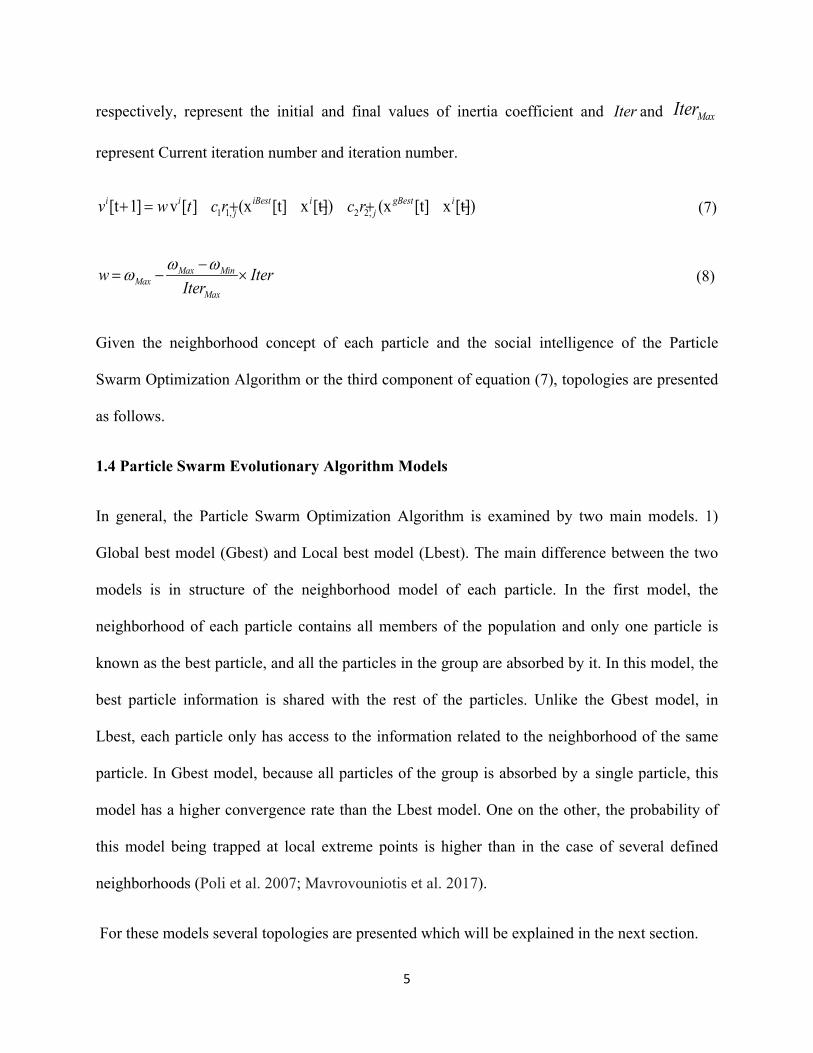
1.5 Types of network topologies or structures
1.5.1 Definition of particle topology
Particle topology is the symbolic network structure of particles that reflects how the population
particles interact and share information with each other.
As mentioned in the previous sections, this algorithm can be defined as a set of particles moving
in areas determined by the best successful experience of each particle and the best experience of
some other particles. According to the phrase "best experience of some other particles”, there are
many structures in the references that three main cases will be discussed below.
1. Star
2. Ring (Circles)
3. Wheel
1.5.2 Star structure
In the star structure, all the particles in the group are adjacent to each other. Therefore, the
position of the best particle of the group is shared with all the particles of the group and affects
their velocity updating equation. This structure is related to the Gbest model. In this structure, the
probability of being trapped at the optimal local point is increased if the best solution of the
problem is not close to the best particle. The properties of this structure can be attributed to its
rapid convergence as well as the greater likelihood of being trapped in optimal local locations.
The star structure is shown in the figure 1.
7
Fig. 1. Star structure
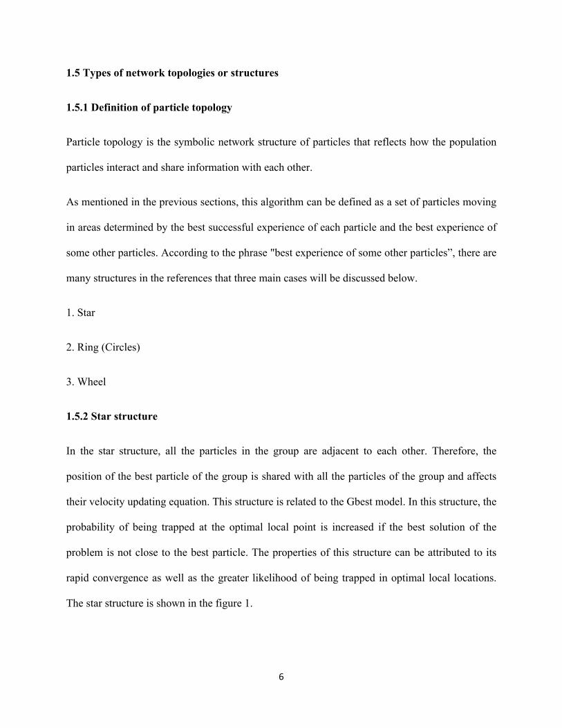
1.5.3 Ring (Circles) structure
In this structure, each particle is adjacent to its n particle. So that there are n/2 particles on each
side. This structure for state n=2 is shown in Fig. (2). In this case, each particle is associated with
its two adjacent particles. This structure is corresponding to the Lbest model. In this structure,
each particle strives to move toward the best particle in its defined neighborhood. In this
structure more areas of the search space are examined, but the convergence rate of this structure
is low (Kacprzyk, 2009).
Fig. 2. Ring structure in n=2
8
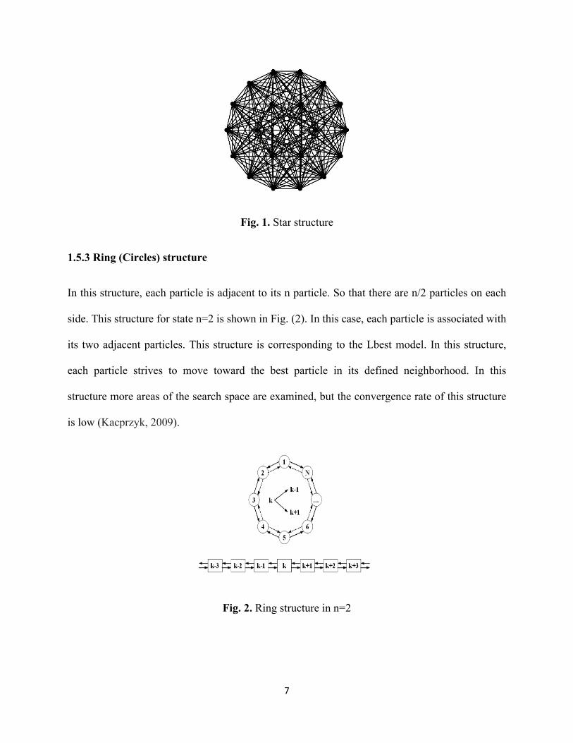
1.5.4 Wheel structure
In the wheel structure, one particle is considered as the Focal particle (Hub). In this structure, the
middle particle is attached to all the particles in the group, but the other particles are only
attached to this particle and are insulated from each other. The focal particle moves to the best
particle. If this focal particle movement improves its performance, it also affects other particles.
This structure is shown in Fig. 3.
Fig. 3. Wheel structure
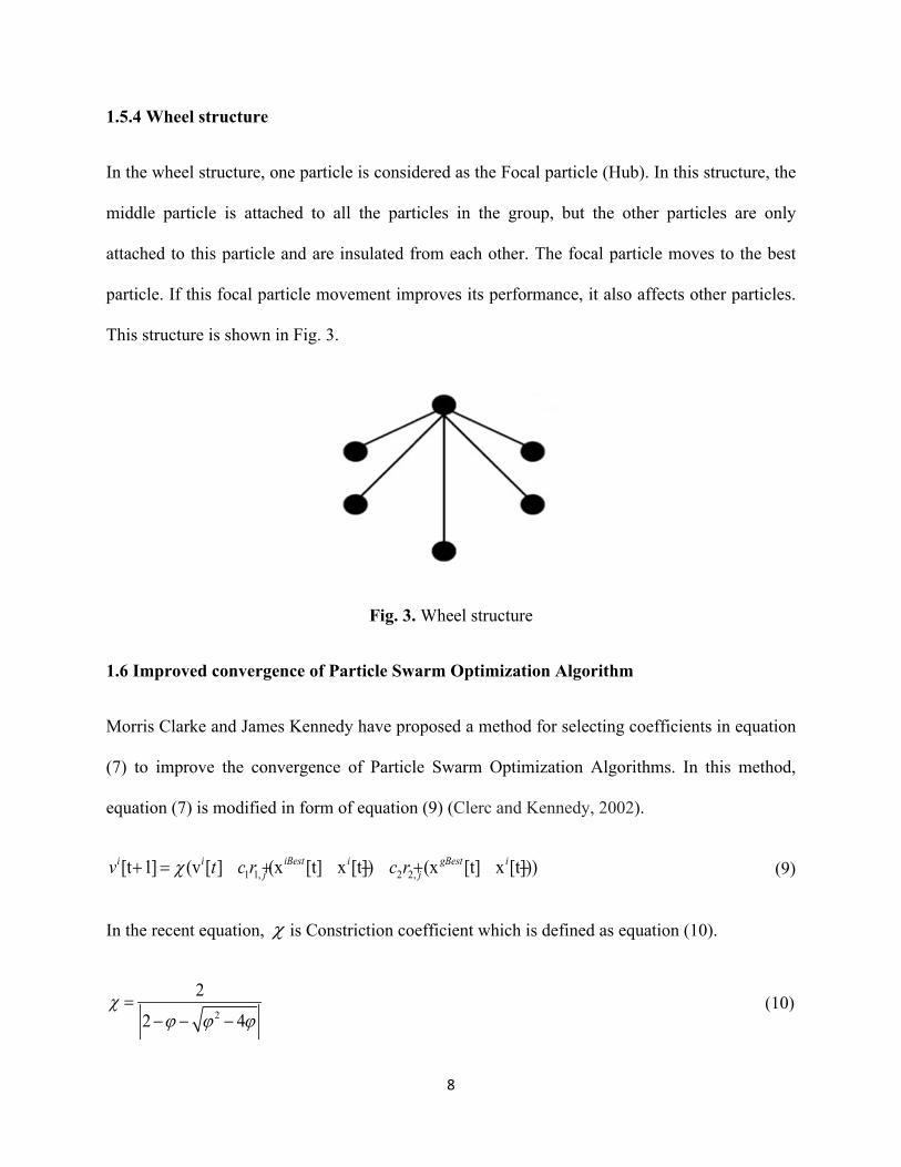
1.6 Improved convergence of Particle Swarm Optimization Algorithm
Morris Clarke and James Kennedy have proposed a method for selecting coefficients in equation
(7) to improve the convergence of Particle Swarm Optimization Algorithms. In this method,
equation (7) is modified in form of equation (9) (Clerc and Kennedy, 2002).
1 1, 2 2,[t 1] (v [ ] (x [t] x [t]) (x [t] x [t]))i i iBest i gBest i
j jv t c r c rχ+ = + − + − (9)
In the recent equation, χ is Constriction coefficient which is defined as equation (10).
2
2
2 4χ
ϕ ϕ ϕ=
− − − (10)
9
In the recent equation, coefficient ϕ is defined as equation 11 (Chan et al. 2007).
1 2 c cϕ ϕ= + > 4 (11)
1.7 Limiting velocity
After obtaining the particle velocity vector of the group, it is necessary to check whether the
velocities obtained are within the specified permissible range. This allowed range is usually
expressed as a coefficient of the width of the search space. This range is shown in Equations (12)
and (13).
max max min( )v x xα= − (12)
min max min( )v x xα= − − (13)
In both recent equations, xmin and xmax represent the variables range in optimization problem. In
addition, Alpha coefficient has a value between zeros to one, so that the velocity threshold value
does not exceed the width of the research space.
After determining the particle velocity vector and determining the particle velocity threshold,
these ranges are applied as relation (14):
,
min min
, , ,
min max
, ,
max max
( 1)
( 1) ( 1) ( 1)
( 1)
i j j
i j i j j i j j
i j i j
v v t v
v t v t v v t v
v v t v
+ ≤
+ = + < + < + ≥
(14)
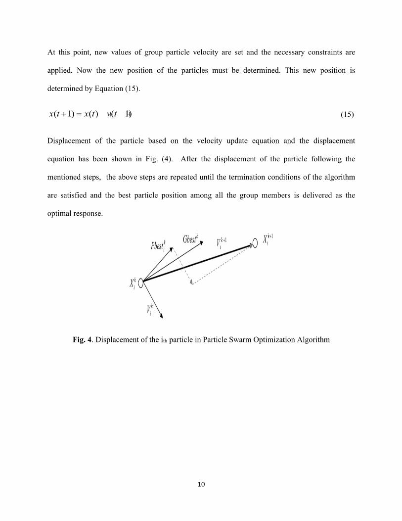
10
At this point, new values of group particle velocity are set and the necessary constraints are
applied. Now the new position of the particles must be determined. This new position is
determined by Equation (15).
( 1) ( ) ( 1)x t x t v t+ = + + (15)
Displacement of the particle based on the velocity update equation and the displacement
equation has been shown in Fig. (4). After the displacement of the particle following the
mentioned steps, the above steps are repeated until the termination conditions of the algorithm
are satisfied and the best particle position among all the group members is delivered as the
optimal response.
Fig. 4. Displacement of the ith particle in Particle Swarm Optimization Algorithm
11
References
Abido, M. A. (2002). Optimal design of power-system stabilizers using particle swarm optimization. IEEE
transactions on energy conversion, 17(3), 406-413.
Bansal, J. C., Singh, P. K., Saraswat, M., Verma, A., Jadon, S. S., & Abraham, A. (2011, October). Inertia weight
strategies in particle swarm optimization. In Nature and Biologically Inspired Computing (NaBIC), 2011 Third
World Congress on (pp. 633-640). IEEE.
Clerc, M. (2010). Particle swarm optimization (Vol. 93). John Wiley & Sons.
Clerc, M., & Kennedy, J. (2002). The particle swarm-explosion, stability, and convergence in a multidimensional
complex space. IEEE transactions on Evolutionary Computation, 6(1), 58-73.
Chan, F. T. S., & Tiwari, M. K (2007). Swarm Intelligence: focus on ant and particle swarm optimization. I-Tech
Education and Publishing. Cited on, 146.
Del Valle, Y., Venayagamoorthy, G. K., Mohagheghi, S., Hernandez, J. C., & Harley, R. G. (2008). Particle swarm
optimization: basic concepts, variants and applications in power systems. IEEE Transactions on evolutionary
computation, 12(2), 171-195.
Di Cesare, N., Chamoret, D., & Domaszewski, M. (2015). A new hybrid PSO algorithm based on a stochastic
Markov chain model. Advances in Engineering Software, 90, 127-137.
Eberhart, R., & Kennedy, J. (1995). A new optimizer using particle swarm theory. In Micro Machine and Human
Science, 1995. MHS'95., Proceedings of the Sixth International Symposium on (pp. 39-43). IEEE.
Eberhart, R. C., Shi, Y., & Kennedy, J. (2001). Swarm Intelligence (The Morgan Kaufmann Series in Evolutionary
Computation).
Kacprzyk, J. (2009). Studies in Computational Intelligence, Volume 198.
Lee, K. Y., & Park, J. B. (2006, October). Application of particle swarm optimization to economic dispatch
problem: advantages and disadvantages. In Power Systems Conference and Exposition, 2006. PSCE'06. 2006 IEEE
PES (pp. 188-192). IEEE.
12
Mavrovouniotis, M., Li, C., & Yang, S. (2017). A survey of swarm intelligence for dynamic optimization:
algorithms and applications. Swarm and Evolutionary Computation, 33, 1-17.
Poli, R., Kennedy, J., & Blackwell, T. (2007). Particle swarm optimization. Swarm intelligence, 1(1), 33-57.
Shi, Y., & Eberhart, R. (1998, May). A modified particle swarm optimizer. In Evolutionary Computation
Proceedings, 1998. IEEE World Congress on Computational Intelligence., The 1998 IEEE International Conference
on (pp. 69-73). IEEE.
Ting, T. O., Shi, Y., Cheng, S., & Lee, S. (2012, June). Exponential inertia weight for particle swarm optimization.
In International Conference in Swarm Intelligence (pp. 83-90). Springer, Berlin, Heidelberg.
Figures
Figure 1
Schematic view of the experimental setup, a) the installed tank on the roof, b) the tank and cylinderinstalled in the laboratory, and c) steel cylinder
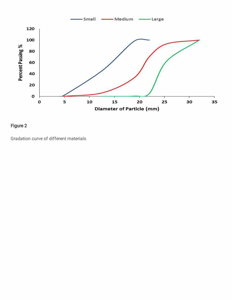
Figure 2
Gradation curve of different materials
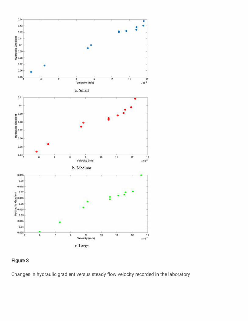
Figure 3
Changes in hydraulic gradient versus steady �ow velocity recorded in the laboratory
Figure 4
Changes in hydraulic gradient versus unsteady �ow velocity recorded in the laboratory
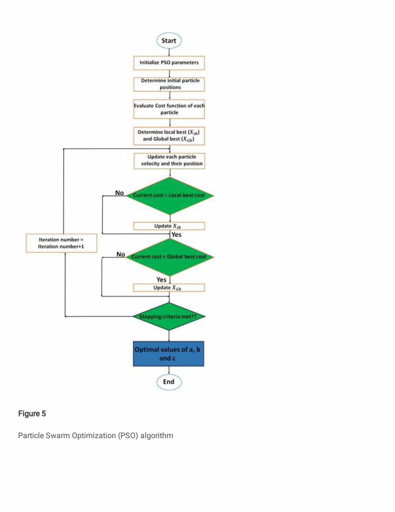
Figure 5
Particle Swarm Optimization (PSO) algorithm
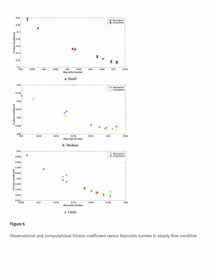
Figure 6
Observational and computational friction coe�cient versus Reynolds number in steady �ow condition

Figure 7
Changes in observational and computational friction coe�cients in terms of Reynolds number inunsteady �ow condition