Embed Size (px)
Citation preview

Article
A joint approach forstrategic bidding of amicrogrid in energy andspinning reserve markets
Gabriella Ferruzzi1, Giorgio Graditi2 andFederico Rossi1
Abstract
In the electricity market, short-term operation is organized in day-ahead and real-time stages.
The two stages that are performed in different time intervals have reciprocal effects on each
other. The paper shows the strategy of a microgrid that participates to both day-ahead energy
and spinning reserve market. It is supposed that microgrid is managed by a prosumer, a decision
maker who manages distributed energy sources, storage units, Information and Communication
Technologies (ICT) elements, and loads involved in the grid. The strategy is formulated consid-
ering that all decisions about the amount of power to sell in both markets and the price links to
the offer, must be taken contextually and at the same time, that is through a joint approach. In
order to develop an optimal bidding strategy for energy markets, prosumer implements a non-
linear mixed integer optimization model: in this way, by aggregating and coordinating various
distributed energy sources, including renewable energy sources, micro-turbines–electricity
power plants, combined heat and power plants, heat production plants (boilers), and energy
storage systems, prosumer is able to optimally allocate the capacities for energy and spinning
reserve market and maximize its revenues from different markets. Moreover, it is considered that
both generators and loads can take part in the reserve market. The demand participation
happens through both shiftable and curtailable loads. Case studies based on microgrid with
various distributed energy sources demonstrate the market behavior of the prosumer using
the proposed bidding model.
Keywords
Ancillary service, microgrid, optimal bidding strategy, joint approach, optimization problem
1University of Naples, Federico II, Naples, Italy2ENEA, Portici, Italy
Corresponding author:
Gabriella Ferruzzi, University of Naples, Federico II, Piazzale Tecchio 80, Naples 80125, Italy.
Email: [email protected]
Energy & Environment
0(0) 1–28
! The Author(s) 2018
Reprints and permissions:
sagepub.co.uk/journalsPermissions.nav
DOI: 10.1177/0958305X18768128
journals.sagepub.com/home/eae
brought to you by COREView metadata, citation and similar papers at core.ac.uk
provided by Archivio della ricerca - Università degli studi di Napoli Federico II

Introduction
Recently power systems have been undergoing changes to satisfy an increasing energydemand. The microgrids (MGs) concept is one of the proposed solutions to cope withthese new challenges. It is based on a cluster of time-varying loads and distributed energysources, a portion of which includes renewable energy sources (RESs). MGs operate assingle controllable system that provides power, and optionally heat, allowing bidirectionalpower to and from the main medium voltage (MV) power grid.1–5
From the system point of view, MGs show the advantages of low investment costs, lowpollutant emission, and high operational flexibility. In addition, the MGs are located at thedemand side, efficiently offering capacities to meet the local requirements.6
Several investigators have analyzed the role played by MGs into the deregulated electric-ity market, their contribution to energy price reduction and to the reliability system increase,as well as their impact on the best strategy devising to minimize operating costs.
The negotiation process between buyers and sellers in a deregulated electricity market isarticulated in different steps: the first is represented by the wholesale energy market and thelast by the ancillary services market, in which imbalances between programmed and realflows are deleted.
Although in literature it is possible to find similar decision support models, participationto both energy markets following a joint approach is an important open research issue.
The objective of this paper is to show how the MG develops an optimalcoordinated bidding strategy for the day-ahead energy and spinning reserve marketstaking into account the “perceived probability.” The perceived probability is related tothe density of probability that reserve is called for. The equilibrium point between thedemand and supply determines the market clearing price (MCP) for each hour MGoffers, for the hours in which the electricity price is high, the power resulting from thedifference between own load and internal production; when the electricity price is low,MG prefers to buy electricity from the main grid in order to satisfy own load. In bothcases the focus is the formulation of an appropriate mathematical optimization model,described in the following.
The model is written in a general and complete manner. It, in fact, considers an MG inwhich both thermal and electrical loads must be satisfied, so that in the MG only electricitypower plants, combined heat and power (CHP) plants, and heat production plants (boilers)are already installed. The presence of thermal and electrical storage systems is alsoaccounted for. Moreover, it is considered that both generators and loads can participatein the reserve market. The demand participation happens through both shiftable and cur-tailable loads.7
Note that a low-voltage MG is characterized by a small amount of total capacity, whilethe market rules generally require that almost a fixed amount of energy must be offered inthe reserve market.8 In order to respect the power limit, we assume that the bid to presentinto the market is a virtual aggregated bid, resulting from the offers of more MGs, formu-lated by each MG in independent way. For this purpose, we hypothesized that prosumeracts as an aggregator on behalf of all.
The remaining of the paper is organized as follows: bidding strategy is discussed in thenext section and formulated in “The model” section; case study in the subsequent section;discussion and conclusion are presented in the final section.
2 Energy & Environment 0(0)

The bidding strategy and literature review
From the MG’s point of view, the energy and the spinning reserve markets are interrelated
and dependent on each other: in fact, as more power is produced for the energy market, as
less it can be produced for the reserve market, and vice versa. It implies to “withhold”
capacity to offer into the energy market and to offer it into reserve market, or “release”
capacity in the energy market and give up to offer it into reserve market.When MG is a producer for the energy market, providing spinning reserve service means
that the value of resultant power delivered to the main grid will be increased; when MG is a
consumer in energy market, the value of resultant power absorbed from the main grid will
be decreased. In all the cases, the MG produces more and/or consumes less energy.Two different dispatching strategies are usually used among markets: sequential and
joint dispatch.In the sequential approach, prosumer takes part in the reserve market only after the
outcomes of the ahead-day market are known offering, eventually, only the residual pro-
duced capacity. However, sequential optimization is more appropriate for simple quantity–
price auctions for both energy and reserve for both energy and reserves but with less efficient
dispatches. In fact, this strategy does not optimize the MG operation obtaining, almost, a
suboptimum solution.9
In the joint approach, the decisions about how much power is to be allocated in each
market and at what price must be taken a priori and contextually. From an economic point
of view, the joint approach provides more efficient dispatches if compared with a sequential
approach, and it is usually proposed to solve auctions where bidders must declare their
units’ technical constraints.9 So, a joint model must explicitly consider, among decision
variables, the powers—those exchanged with the main grid and those generated by each
unit, and the curtailable loads, for both markets. These decision variables are added to the
shiftable loads and to the levels and powers of the storages.It said the joint approach provides more efficient dispatches if compared with a sequen-
tial approach, and it is usually proposed to solve auctions where bidders must declare their
units’ technical constraints.9
The participation of the reserve market involves that the benefits for MG can increase.The amount of the additional revenues depends on the way in which reserve payments
are made.More specifically, there are markets in which the reserve power is paid at reserve price,
only when reserve is actually used. In others, the reserve power is paid, at reserve price, when
reserve is allocated but not used, and, at energy price, when the reserve is used.10–12
The problem considered in this paper was dealt with in literature almost from the point of
view of traditional generation companies13 or the virtual power plant (VPP),14,15 using
sequential models16–21 or joint model.6,22–32
In Ferruzzi et al.33 an arbitrage strategy for VPPs by participating in energy, spinning
reserve, and reactive power markets is presented. In Rossi,4 a risk-averse optimal offering
model for a VPP is proposed in the joint energy and reserve markets.However, papers that address the problem with reference or MGs exist in the litera-
ture6,34,35 although in most of the studies, only the first stage of energy management has
been considered.13–15,36–38 This probably happens because MG is characterized by a small
Ferruzzi et al. 3

amount of total capacity, while the market rules generally require that almost a fixed
amount of energy must be offered in the reserve market.In this work, indeed, the main differences can be summarized as follows: participation of
an MG grid connected mode in both the energy markets by a prosumer. It takes part in the
markets both as producer and consumer according to energy price values, internal load and
grid constraints. The participation also in the reserve market introduces an additional level
of complexity in the MG operation but offers the potential for additional revenue. In order
to respect the MG power limits, authors assume that the bid to present into the market is an
aggregated bid, resulting from the offers of more MGs.39 For this purpose, we hypothesized
that prosumer acts as an aggregator on behalf of all. The study is developed with reference
to the Italian framework. Moreover, an optimization model to minimize the operation costs
of an MG in the presence of uncertainties is shown: different from the others presented in
literature, it takes into account not only the uncertainties from RESs, but also the uncer-
tainties linked to the different energy prices. Authors underline that none of the last citied
works formulate a model that allows to deal with together the cases of the call and of the not
call the reserve: this is particularly relevant when intertemporal constraints exist (i.e. as those
introduced by shiftable loads and storage systems).In particular, authors assume that a “perceived probability”, rt, that reserve is called, is
equal to 0 (MG does not take part in reserve market) or to 1 (the MG takes part in the
reserve market).The perceived probability is related to the density of probability that the reserve is called,
obtained by analyzing historical series, different from hour to hour.Furthermore, none of the citied works considers the cogeneration and none treats shift-
able loads.
The model
A novel model of day energy and reserve management of MG is proposed. It formulates a
nonlinear mixed integer programming model to evaluate how MG develops an optimal
bidding strategy in energy markets. The optimal management problem consists in research-
ing, hour by hour during the day, the values of energy exchanged with the main distribution
network, the energy production of each dispatchable unit, the energy charged to/discharged
from the storage units, and the controllable load profiles that optimize an economic objec-
tive. Also the choices of the thermoelectric units that must be in operation on an hourly base
and the determination of the internal network status consistent with operating constraints
are part of the problem.The optimization is extended simultaneously to all 24 h of the management period
because the presence of storage systems and shifting actions introduce intertemporal
constraints.It is assumed that all different production units (generators and cogenerators as well as
the curtailable loads) have the requirements to provide reserve service; the load shedding is
used also for the energy market; the MG can estimate fixed loads, RES production, and
prices of energy and spinning reserve markets for each hour through the analysis of time
series; the MG knows the density of probability that the reserve will be called to produce,
which, according to Yamin,28 and contrary to Bai et al.,16 Chitkara et al.,17 and Jia et al.18
has different values from hour to hour.
4 Energy & Environment 0(0)

Objective function
The revenues, R, are related to energy sold in the reserve market and, if there is, in the
energy market. Neglecting the management costs of storage and shifting, the costs, C, are
related, instead, to the energy bought from the main grid, if there is, to production costs of
generators, cogenerators, and boilers and, finally, to load shedding.That said, assuming that the exchanged power in the energy market is positive if it is
bought and negative if it is sold, and assuming that the energy market price is equal in the
buying and selling phases, the objective function to maximize is
E R� Cð Þ ¼X24t¼1
rtqrtP
rgridt þ
X24t¼1
qetPegridt �
X24t¼1
1� rtð ÞXj2XC
Ccj PeCet;j
� �"
þXj2XB
CBjPBt;j
� �þ Xj2XGj
CGjPeGt;j
� �þX
j2XDCU
CDCUjPeDCUt;j
� �#
�X24t¼1
rtð ÞXj2XC
Ccj PeCet;j
þ PrCet;j
� �þXj2XB
CBjPBt;j
� �"
þXj2XG
CGjPeGt;j
þ PrGt;j
� �þX
j2XDCU
CDCUjPeDCUt;j
þ PrDCUt;j
� �#(1)
The first summation of equation (1) represents the revenue, Rr derived from the partic-
ipation to the reserve market, supposing that the reserve power is paid, at reserve price only
when reserve is actually used.If, moreover, the reserve power is paid, at reserve price, when reserve is allocated but not
used, and, at energy price, when the reserve is used, it must be changed in
EðRrÞ ¼X24t¼1
½ð1� rtÞqr þ rtqe�Pr
gridt
Constraints
The basic equality constraints are the thermal and electric balance constraints.Assuming that the storage powers are positive during the discharge and negative during
the charge, they area
1� rtð ÞXj2XC
PeCet;j
gjþX
j2XBPBt;j
!þ rt
Xj2XC
PeCet;j
gjþXj2XC
PrCet;j
gjþXj2XB
PBt;j
!
¼Xj2XDth
PDsht;j þXj2XST
PSTt;jt ¼ ð1 . . . :24Þ
(2)
Ferruzzi et al. 5

X24t¼1
1� rtð Þ�XX
j2Xc
PeGt;j
þ PrCet;j
� �þ Pe
gridt �Xj2XDF
PDFt;j
þXj2XDC
PeDCUt;j
�X
j2XDSH
PDSHt;j�Xj2XSE
PSEt;j
�
þX24t¼1
r
�X24t¼1
PeCet;j
þ PrCet;j
þXj2XG
PeGt;j
þXj2XG
PrGt;j
þ Pegridt
þ Pegridt �
Xj2XDF
PDFt;jþXj2XDC
PeDCUt;j
þXj2XDC
PrDCUt;j
�X
j2XDSH
PDSHt;j�Xj2XSE
PSEt;j
�t ¼ ð1 . . . :24Þ
(3)
In equation (3) PDSHt,j is the shifted power of the jth shiftable load.The relationship between the loads before and after shifting can be represented by intro-
ducing binary variables ut,j.The condition ut,j¼ 1 identifies the initial interval t where the jth shiftable load starts to be
supplied for the next Sj hours. Considering that the profile of the jth shiftable load startsonly once, only a binary variable can be equal to one. Moreover, only the first (Tj�Sjþ 1)binary variables can be defined because each ut,j variable is associated with the next (Sjþ 1)variables PDSHt,j
It must happen that
XTj�Sjþ1
t¼1
ut;j ¼ 1ðj2DSHÞ (4)
Then, let us consider that only the variables associated with ut,j¼ 1, i.e.PDSHt;j
;PDSHtþ1;j; ; . . . ;PDSHtþk;j
, take positive values. Specifically, each PDSHt;jj with
k¼ t� sþ 1, takes the value DSHt;j. This way, the links between shiftable and shiftedloads are
PDSHt;j¼Xts¼1
DSHðt�kþ1Þ � uk;j ðj2DSH; t ¼ 1; . . . ;Tj � Sj þ 1Þ (5)
Mathematically the problem is a nonlinear mixed integer programming problem.However, if the shiftable loads are not taken into account, it becomes an easier nonlinearprogramming problem.
When there are storage units, the objective function is the same because the operationcosts of storage can be neglected.
6 Energy & Environment 0(0)
Additional equality constraints can be derived from modeling the storage units. In fact, itis necessary to express the variation of the storage levels and the restoration of the initiallevels as: the variation of the storage levels
WSEt;j¼ WSEt�1;j
þ PSEt;jðj2XSE; t ¼ 1; . . . ; 24Þ (6a)
WSTt;j¼ WSTt�1;j
þ ksjPSTt;jðj2XSE; t ¼ 1; . . . ; 24Þ (6b)
Finally, inequality constraints express the limits on internal production and maximumamount of exchangeable power, bought or sold, in the main grid must be considered:
• limits on cogenerators production
0 � PrCej
� PMaxCej
� PeCej
� �ðj2XC; t ¼ 1; . . . ; 24Þ (7a)
PeCej
þ PrCej
� PMaxCej
ðj2XC; t ¼ 1; . . . ; 24Þ (7b)
• limits on boilers production
PmBj
� PBt;j� PM
Bjðj2XC; t ¼ 1; . . . ; 24Þ (8)
• limits on generators production
0 � PrGt;j
� PMaxGj
� PeGj
� �ðj2XG; t ¼ 1; . . . ; 24Þ (9a)
PeGt;j
þ PrGt;j
� PMaxGj
ðj2XG; t ¼ 1; . . . ; 24Þ (9b)
• limits if exchangeable power in the main grid
�PMaxgridt
� Pgridt � PMaxgridt
ðt ¼ 1; . . . ; 24Þ (10)
It is noted that the model does not evaluate the arbitrage opportunities: MG cannot buymore energy in the energy market to sell more into the reserve market. If arbitrage isadmitted, constraints (7) and (9) must be written as
0 � PrCej
� PMaxCej
� PeCej
� �ðj2XC; t ¼ 1; . . . ; 24Þ (11a)
0 � PrGt;j
� PMaxGj
� PminGj
� �ðj2XG; t ¼ 1; . . . ; 24Þ (11b)
Ferruzzi et al. 7

Case study
The model described in Siano et al.1 is applied to a residential MG, grid connected, com-posed of different entities, i.e. hotel, sports center, markets, offices, and buildings. Thermaland electric total loads, with reference to a summer day, are reported in Table 1. The loadsare reduced by the renewable energy.
Some loads can be shifted, so it is possible moving them from peak load to valley load.Washing machines, dryers, dishwasher, air conditioners, irons, and electric coffee makersare shiftable loads. The total number of devices taken into account for the analysis is 1260and their characteristics are reported in Table 2.
In MG there are six power generators: two power plants producing only electricity (G1,G2) and four producing electricity and heat (Ce1, Ce2, Ce3, Ce4). To satisfy thermal loads,there is also a boiler.
The generator and cogenerators cost functions are assumed quadratic, while the boilercost function is assumed to be linear as follows
CCjðPCet;jÞ ¼ aCjP
2Cet;j
þ bCjPCet;j þ cCj
CGjðPCet;jÞ ¼ aGjP
2Cet;j
þ bGjPCet;j þ cGj
Table 1. Hourly electrical and thermal loads.
Hours [h] PDet ½kWe� PDth½kWe�1 440.0 320.0
2 440.0 295.0
3 440.0 275.0
4 440.0 275.0
5 440.0 495.0
6 740.0 605.0
7 1200.0 1305.0
8 1905.0 3560.0
9 2345.0 3570.0
10 2405.0 3690.0
11 2420.0 3625.0
12 2440.0 4095.0
13 2470.0 4125.0
14 2465.0 4300.0
15 2450.0 4255.0
16 2395.0 3950.0
17 2360.0 3905.0
18 2335.0 3605.0
19 1695.0 1695.0
20 1425.0 1680.0
21 1295.0 1425.0
22 955.0 1020.0
23 530.0 520.0
24 425.0 390.0
8 Energy & Environment 0(0)

CBjðPBt;j
Þ ¼ bCjPBjþ cBj
Technical and economic characteristics of the generators and cogenerators are reportedin Table 2; in particular are reported the minimum and maximum power of each unit andthe coefficients aCj, bCj, cCj, aGj, bGj, and cCj. Instead, the maximum power of boiler is4500 kW and the coefficient bj is equal to 55.0.
In Table 3, energy and spinning reserve market prices are reported. They are available online on the Gestore dei Mercati Energetici website (www.mercatoelettrico.org).
Table 2. Technical and economic characteristics of the generation power plants.
Units PmGj½kW� PMGj
½kW� cGj½e� bGj
½e=MWh� aGj½e=MWh
2� Pmcej ½kW� Pmcej ½kW� cCej ½e� bCej ½e=MWh� aCej ½e=MWh2�
G1 36.0 180.0 892.0 25.8 0.021
G2 36.0 180.0 892.0 33.4 0.042
Ce1 80.0 400.0 1017.0 10.4 0.0005
Ce2 80.0 400.0 1017.0 22.7 0.0005
Ce3 10.0 80.0 484.0 48.1 0.105
Ce4 10.0 80.0 840.0 54.2 0.233
Table 3. Energy and spinning reserve market prices.
Hours [h] qet ½e� qrt ½e�1 41.7 48.0
2 39.7 45.7
3 38.0 43.8
4 36.0 41.4
5 36.0 41.5
6 36.0 41.4
7 39.8 45.8
8 44.6 51.3
9 49.5 56.9
10 51.8 59.6
11 46.3 53.3
12 40.8 47.0
13 39.3 45.2
14 38.5 44.2
15 43.7 50.2
16 42.0 48.3
17 44.9 51.6
18 48.3 55.5
19 44.5 51.1
20 45.0 51.8
21 55.0 63.3
22 59.4 68.3
23 55.0 63.3
24 50.7 58.3
Ferruzzi et al. 9

The model, described in Siano et al.,1 was implemented for different configurations. It issupposed, first of all, that all loads are fixed and that all units (cogenerators and generators)produce only electricity, so that only the boiler satisfies the thermal load. In this configu-ration, two cases are analyzed that correspond to a perceived probability rt, that the reserveis not called to produce or, instead, is called to produce: rt¼ r¼ 0 (case 1) and rt¼ r¼ 1(case 2).
It is then considered the cogeneration always assuming the presence only of fixed loads.Also in this configuration are considered the cases rt¼ r¼ 0 (case 3) and rt¼ r¼ 1 (case 4).
The cases 5, 6, and 7 consider always the cogeneration, but a percentage of the loads issupposed to be shiftable. Now, in addition to cases rt¼ r¼ 0 (case 5) and rt¼ r¼1 (case 6), itis also considered the case in which the probability is not constant, assuming the value 0 or 1depending on the interval (case 7).
It is finally also examined the configuration in which is present a storage system for r¼ 0(case 8) and r¼ 1 (case 9). For the eight cases considered, the model was implemented in theversion that does not provide the possibility of arbitrage, i.e. the possibility that MG buys inthe electricity energy market only in order to sell it in the reserve market. In the following,
however, some examples will be provided to show what would be the benefit if the arbitragewas permitted.
Yet, for all the cases analyzed, the revenue from the participation in reserve market iscalculated taking into account that reserve is paid, at reserve price, only when reserve is
actually used.
Not_cogeneration
In Table 4 are reported results for rt¼0.
• the powers produced and power exchanged with main grid are internal to the domain,• the units produce until their marginal costs (that vary in the ranges reported in Table 5)
reach the electricity market price (see G2, for example, in hours 1, 2, 3, 7, 8).
If units with marginal cost are higher of electricity market price produced, it means thatthe constraint related to the maximum energy exchanged with the main grid (assumed equalto 1200 kW) is reached: MG cannot withdraw more from the main grid and the unitsproduced, according to the criterion of increasing marginal costs, until the balance con-straint is satisfied (this happens, for example, at the units Ce3 and Ce4 in hours 12–15).
It is important to note that MG is producer in the hours 1–6 and 22–24, while it isconsumer in the hours 7–21, according to how internal production is related to internalconsumption.
Different are the operating results for r¼ 1, as shown in Table 6 which now lists also thequantity relating to the reserve market.
MG tends to take part also in the reserve market, being the reserve market price alwayshigher than electricity market price (MCP).
In the intervals in which the power exchanged Pegridt is not bound to the maximum
value, all the units offer the minimum power into the energy market.Those that have the marginal cost are always lower than the reserve price (G1, G2, Ce1,
and Ce2) sell to the reserve market the residual capacity; the units that, indeed, have mar-ginal cost always greater than reserve price (Ce3 and Ce4) do not offer in the reserve market.
10 Energy & Environment 0(0)

As said before, this is true until the power exchanged with the main grid is not at maximum.When it happens, (see 8–19 h) the units, even those with marginal cost higher than marketprice, are obliged to produce in the electricity market in order to respect the balance con-straint and produce respecting the criterion of increasing marginal costs. It is noted that inthe intervals 1–6 and 22–24, contrary to the case 1, MG prefers to buy in the electricitymarket in order to have the opportunity to sell more in the reserve market.
The just commented results are completely different from those that would obtain byfollowing the sequential approach rather than the proposed joint approach.
Table 4. Not cogeneration with r¼ 0. Case 1.
Hours [h] qe½2� PDet ½kWe� PeGt;1½kWe� PeGt;2
½kWe� Pecet;1 ½kWe� Pecet;2 ½kWe� Pecet;3 ½kWe� Pecet;4 ½kWe� Pegridt ½kWe�1 41.7 440.0 180.0 87.1 400.0 400.0 10.0 10.0 �647.1
2 39.7 440.0 180.0 63.3 400.0 400.0 10.0 10.0 �623.3
3 38.0 440.0 180.0 43.6 400.0 400.0 10.0 10.0 �603.6
4 36.0 440.0 180.0 36.0 400.0 400.0 10.0 10.0 �596.0
5 36.0 440.0 180.0 36.0 400.0 400.0 10.0 10.0 �596.0
6 36.0 740.0 180.0 36.0 400.0 400.0 10.0 10.0 �296.0
7 39.8 1200.0 180.0 64.4 400.0 400.0 10.0 10.0 135.6
8 44.6 1905.0 180.0 121.1 400.0 400.0 10.0 10.0 783.9
9 49.5 2345.0 180.0 180.0 400.0 400.0 10.0 10.0 1165.0
10 51.8 2405.0 180.0 180.0 400.0 400.0 35.0 10.0 1200.0
11 46.3 2420.0 180.0 180.0 400.0 400.0 50.0 10.0 1200.0
12 40.8 2440.0 180.0 180.0 400.0 400.0 60.0 20.0 1200.0
13 39.3 2470.0 180.0 180.0 400.0 400.0 60.0 50.0 1200.0
14 38.5 2465.0 180.0 180.0 400.0 400.0 60.0 45.0 1200.0
15 43.7 2450.0 180.0 180.0 400.0 400.0 60.0 30.0 1200.0
16 42.0 2395.0 180.0 160.0 400.0 400.0 25.0 10.0 1200.0
17 44.9 2360.0 180.0 164.9 400.0 400.0 10.0 10.0 1200.0
18 48.3 2335.0 180.0 119.6 400.0 400.0 10.0 10.0 1170.1
19 44.5 1695.0 180.0 126.2 400.0 400.0 10.0 10.0 575.4
20 45.0 1425.0 180.0 180.0 400.0 400.0 10.0 10.0 298.8
21 55.0 1295.0 180.0 180.0 400.0 400.0 32.9 10.0 92.1
22 59.4 955.0 180.0 180.0 400.0 400.0 53.8 11.2 �270.0
23 55.0 530.0 180.0 180.0 400.0 400.0 32.9 10.0 �672.9
24 50.7 425.0 180.0 180.0 400.0 400.0 12.5 10.0 �757.5
Table 5. Marginal costs in correspondence of minimum and maximumpower produced.
Units kjm kjM
G1 27.3 33.3
G2 37.4 49.5
Ge1 10.4 10.8
Ge2 23.1 24.8
Ge3 50.2 60.7
Ge4 58.9 82.1
Ferruzzi et al. 11

Table
6.Notcogenerationwithr¼1.
Hours
[h]
qe t
[e]
P De t
[kW
e]
Pe Gt;1
[kW
e]
Pe Gt;2
[kW
e]
Pe cet;1
[kW
e]
Pe cet;2
[kW
e]
Pe cet;3
[kW
e]
Pe cet;4
[kW
e]
Pe gridt
[kW
e]
Pr t2
Pr Gt;1
[kW
e]
Pr Gt;2
[kW
e]
Pr Ce t;1
[kW
e]
Pr Ce t;2
[kW
e]
Pr Ce t;3
[kW
e]
Pr Ce t;4
[kW
e]
Pr gridt
[kW
e]
141.7
440
36.0
36.0
80.0
80.0
35.0
10.0
188.0
48.0
144.0
144.0
320.0
320.0
0.0
0.0
�928.0
239.7
440
36.0
36.0
80.0
80.0
10.0
10.0
188.0
45.7
144.0
144.0
320.0
320.0
0.0
0.0
�928.0
338
440
36.0
36.0
80.0
80.0
10.0
10.0
188.0
43.8
144.0
111.5
320.0
320.0
0.0
0.0
�895.5
436
440
36.0
36.0
80.0
80.0
10.0
10.0
188.0
41.4
144.0
83.0
320.0
320.0
0.0
0.0
�867.0
536
440
36.0
36.0
80.0
80.0
10.0
10.0
188.0
41.5
144.0
84.6
320.0
320.0
0.0
0.0
�868.6
636
740
36.0
36.0
80.0
80.0
10.0
10.0
488.0
41.4
144.0
83.0
320.0
320.0
0.0
0.0
�867.3
739.8
1200
36.0
36.0
80.0
80.0
10.0
10.0
948.0
45.8
144.0
144.0
320.0
320.0
0.0
0.0
�928.0
844.6
1905
36.0
145.0
400.0
213.0
10.0
10.0
1200.0
51.3
144.0
144.0
0.0
187.0
15.0
0.0
�490.0
949.5
2345
180.0
180.0
400.0
400.0
10.0
10.0
1200.0
56.9
0.0
35.0
0.0
0.0
42.0
5.9
�82.9
10
51.8
2405
180.0
180.0
400.0
400.0
35.0
10.0
1200.0
59.6
0.0
0.0
0.0
0.0
25.6
11.6
�36.6
11
46.3
2420
180.0
180.0
400.0
400.0
50.0
10.0
1200.0
53.3
0.0
0.0
0.0
0.0
10.0
0.0
�10.0
12
40.8
2440
180.0
180.0
400.0
400.0
60.0
20.0
1200.0
47.0
0.0
0.0
0.0
0.0
0.0
0.0
0.0
13
39.3
2470
180.0
180.0
400.0
400.0
60.0
50.0
1200.0
45.2
0.0
0.0
0.0
0.0
0.0
0.0
0.0
14
38.5
2465
180.0
180.0
400.0
400.0
60.0
45.0
1200.0
44.2
0.0
0.0
0.0
0.0
0.0
0.0
0.0
15
43.7
2450
180.0
180.0
400.0
400.0
60.0
30.0
1200.0
50.2
0.0
0.0
0.0
0.0
0.0
0.0
0.0
16
42
2395
180.0
180.0
400.0
400.0
25.0
10.0
1200.0
48.3
0.0
0.0
0.0
0.0
1.0
0.0
�1.0
17
44.9
2360
180.0
160.0
400.0
400.0
10.0
10.0
1200.0
51.6
0.0
20.0
0.0
0.0
16.6
0.0
�36.6
18
48.3
2335
180.0
135.0
400.0
400.0
10.0
10.0
1200.0
55.5
0.0
45.0
0.0
0.0
35.2
2.8
�83.0
19
44.5
1695
36.0
36.0
323.0
80.0
10.0
10.0
1200.0
51.1
144.0
144.0
77.0
320.0
14.4
0.0
�699.4
20
45
1425
36.0
36.0
80.0
80.0
10.0
10.0
1173.0
51.8
144.0
144.0
320.0
320.0
17.4
0.0
�945.4
21
55
1295
36.0
36.0
80.0
80.0
10.0
10.0
1043.0
63.3
144.0
144.0
320.0
320.0
19.4
0.0
�997.4
22
59.4
955
36.0
36.0
80.0
80.0
10.0
10.0
703.0
68.3
144.0
144.0
320.0
320.0
50.0
31.5
�1009.5
23
55
530
36.0
36.0
80.0
80.0
10.0
10.0
278.0
63.3
144.0
144.0
320.0
320.0
50.0
19.4
�997.4
24
50.7
425
36.0
36.0
80.0
80.0
10.0
10.0
173.0
58.3
144.0
144.0
320.0
320.0
50.0
9.0
�987.0
12 Energy & Environment 0(0)

Cogeneration
Typical cogeneration plants (CHP) are driven by the thermal demand and the systems are
dimensioned for thermal base load: that means they operate continuously for many hours of
the year. In this work in which CHPs take part to the energy market, several possibilities can
be realized, related to the variable energy price. Consequently, the output power of CHP
units could be between the technical minimum and maximum rates.In Table 7 are reported the operating results for r¼ 0.In this case, for the cogenerators, the criterion of increasing marginal costs requires that
the cogenerators work until their marginal costs reach the value given by the sum of the
electricity market price and the ratio between the marginal cost of boiler and the efficiency
of cogeneration (the latter assumed equal to 0.8 for all the cogenerators). But this value is
never achieved in our case due to high marginal cost of boiler. In comparison to the case 1,
in the intervals 1–6 and 23–24, since the thermal load is low, the cogenerators with lower
marginal costs reduce the production and the cogenerators with higher marginal costs con-
tinue to work at minimum. Differently, the generators work at maximum. In the other
intervals, characterized by higher thermal loads, all units produce at maximum, resulting
in that the maximum value of the power exchanged with main grid is never reached. As in
the case 1, MG sells in the intervals.The total power produced by each unit remains the same as the case 3, but it is distributed
in the two markets taking into account the balance constraints and the prices. In the
intervals in which Pegridt does not reach the maximum, all the units offer the minimum
power into the electricity market and offer as much as possible in the reserve market. Note
that, for example, as G2 does not sell, as in the case 2, the residual capacity: the thermal load
is low and, to satisfy it, it is sufficient that produce Ce5 and Ce6, that in the energy market
are constrained to produce the minimum and G1, which has a lower marginal cost than G2.
As in the case 2, when the power exchanged with main grid reaches their maximum (see 8–
19 h), the units, even those with marginal cost higher than market price, are obliged to
produce in the energy market if that is necessary to respect the balance constraint. As in the
case 2 and contrary to the case 3, in the intervals 1–6 and 22–24, MG prefers to buy in the
energy market in order to have the opportunity to sell more in the reserve market. The just
commented results are completely different from those that would be obtained by following
the sequential approach rather than the proposed joint approach.Tables 8 and 9 show electrical and thermal quantities, respectively, in case of cogenera-
tion and r¼ 1.
Shiftable loads
Table 10 shows the characteristics of the shiftable loads considered. More precisely, it shows
the type of loads, the cycle duration of each load, the shiftable power of each load in the
hourly intervals.Each load is composed by a number Nj of devices, each of power dSHs (Table 11). In
Tables 12 and 13 are reported the results for r¼ 0; in Tables 14 and 15 those for r¼ 1. In
particular, the first Tables 12 and 13 show the position preshift and postshift of the loads;
the second Table 14 the complete state of the MG postshift.As we can easily see, the analysis of the tables shows that each load is shifted, if own Tj
allows, in the time intervals equal in number to the hours of Sj—to which corresponds the
Ferruzzi et al. 13

Table
7.Cogenerationwithr¼0.
Hour
[h]
qe t
[e]
P De t
[kW
e]
Pe Gt;1
[kW
e]
Pe Gt;2
[kW
e]
Pe cet;1
[kW
e]
Pe cet;2
[kW
e]
Pe cet;3
[kW
e]
Pe cet;4
[kW
e]
Pe gridt
[kW
e]
P Dth
[kW
e]
P Gtht;1
[kW
e]
P Gth
t;2
[kW
e]
P Cth
t;1
[kW
th]
P Cth
t;2
[kW
th]
P Cth
t;3
[kW
th]
P Cth
t;4
[kW
th]
P Bt
[kW
th]
141.7
440
180.0
180.0
212.0
80.0
10.0
10.0
�232.0
320.0
00
265.0
100.0
12.5
12.5
0.0
239.7
440
180.0
180.0
156.0
80.0
10.0
10.0
�176.0
295.0
00
195.0
100.0
12.5
12.5
0.0
338
440
180.0
180.0
136.0
80.0
10.0
10.0
�156.0
275.0
00
170.0
100.0
12.5
12.5
0.0
436
440
180.0
180.0
120.0
80.0
10.0
10.0
�140.0
275.0
00
150.0
100.0
12.5
12.5
0.0
536
440
180.0
180.0
120.0
80.0
10.0
10.0
�140.0
495.0
00
150.0
100.0
12.5
12.5
0.0
636
740
180.0
180.0
296.0
80.0
10.0
10.0
�16.0
605.0
00
370.0
100.0
12.5
12.5
0.0
739.8
1200
180.0
180.0
384.0
80.0
10.0
10.0
356.0
1305.0
00
480.0
100.0
12.2
12.5
0.0
844.6
1905
180.0
180.0
400.0
400.0
60.0
60.0
625.0
3560.0
00
500.0
100.0
75.0
75.0
200.0
949.5
2345
180.0
180.0
400.0
400.0
60.0
60.0
1065.0
3570.0
00
500.0
500.0
75.0
75.0
2410.0
10
51.8
2405
180.0
180.0
400.0
400.0
60.0
60.0
1125.0
3690.0
00
500.0
500.0
75.0
75.0
2540.0
11
46.3
2420
180.0
180.0
400.0
400.0
60.0
60.0
1140.0
3625.0
00
500.0
500.0
75.0
75.0
2475.0
12
40.8
2440
180.0
180.0
400.0
400.0
60.0
60.0
1160.0
4095.0
00
500.0
500.0
75.0
75.0
2945.0
13
39.3
2470
180.0
180.0
400.0
400.0
60.0
60.0
1190.0
4125.0
00
500.0
500.0
75.0
75.0
2975.0
14
38.5
2465
180.0
180.0
400.0
400.0
60.0
60.0
1185.0
4300.0
00
500.0
500.0
75.0
75.0
3150.0
15
43.7
2450
180.0
180.0
400.0
400.0
60.0
60.0
1170.0
4255.0
00
500.0
500.0
75.0
75.0
3105.0
16
42
2395
180.0
180.0
400.0
400.0
60.0
60.0
115.0
3950.0
00
500.0
500.0
75.0
75.0
2800.0
17
44.9
2360
180.0
180.0
400.0
400.0
60.0
60.0
1080.0
3905.0
00
500.0
500.0
75.0
75.0
2755.0
18
48.3
2335
180.0
180.0
400.0
400.0
60.0
60.0
1055.0
3605.0
00
500.0
500.0
75.0
75.0
1455.0
19
44.5
1695
180.0
180.0
400.0
400.0
60.0
60.0
415.0
1695.0
00
500.0
500.0
75.0
75.0
1455.0
20
45
1425
180.0
180.0
400.0
400.0
60.0
60.0
145.0
1680.0
00
500.0
500.0
75.0
75.0
545.0
21
55
1295
180.0
180.0
400.0
400.0
60.0
60.0
15.0
1425.0
00
500.0
500.0
75.0
75.0
530.0
22
59.4
955
180.0
180.0
400.0
400.0
60.0
60.0
�325.0
1020.0
00
500.0
500.0
75.0
75.0
275.0
23
55
530
180.0
180.0
400.0
396.0
10.0
10.0
�646.0
520.0
00
500.0
495.0
12.5
12.5
0.0
24
50.7
425
180.0
180.0
316.0
80.0
10.0
10.0
�351.0
390.0
00
395.0
100.0
12.5
12.5
0.0
14 Energy & Environment 0(0)

Table
8.Cogenerationwithr¼1.Electricalquantities.
Hours
[h]
qe t
[e]
P De t
[kW
e]
Pe Gt;1
[kW
e]
Pe Gt;2
[kW
e]
Pe cet;1
[kW
e]
Pe cet;2
[kW
e]
Pe cet;3
[kW
e]
Pe cet;4
[kW
e]
Pe gridt
[kW
e]
Pr t [kW
e]
Pr Gt;1½2�
Pr Gt;2
[kW
e]
Pr Ce t;1
[kW
e]
Pr Ce t;2
[kW
e]
Pr Ce t;3
[kW
e]
Pr Ce t;4
[kW
e]
141.7
440.0
36.0
36.0
80.0
80.0
10.0
10.0
188.0
48.0
144.0
144.0
132.0
0.0
0.0
0.0
239.7
440.0
36.0
36.0
80.0
80.0
10.0
10.0
188.0
45.7
144.0
144.0
76.0
0.0
0.0
0.0
338.0
440.0
36.0
36.0
80.0
80.0
10.0
10.0
188.0
43.8
144.0
111.5
56.0
0.0
0.0
0.0
436.0
440.0
36.0
36.0
80.0
80.0
10.0
10.0
188.0
41.4
144.0
83.0
40.0
0.0
0.0
0.0
536.0
440.0
36.0
36.0
80.0
80.0
10.0
10.0
188.0
41.5
144.0
84.6
40.0
0.0
0.0
0.0
636.0
740.0
36.0
36.0
80.0
80.0
10.0
10.0
488.0
41.4
144.0
83.0
216.0
0.0
0.0
0.0
739.8
1200.0
36.0
36.0
80.0
80.0
10.0
10.0
948.0
45.8
144.0
144.0
304.0
0.0
0.0
0.0
844.6
1905.0
36.0
145.0
400.0
213.0
10.0
10.0
1200.0
51.3
144.0
144.0
304.0
0.0
0.0
0.0
949.5
2345.0
180.0
180.0
400.0
400.0
10.0
10.0
1200.0
56.9
0.0
35.0
0.0
0.0
50.0
50.0
10
51.8
2405.0
180.0
180.0
400.0
400.0
35.0
10.0
1200.0
59.6
0.0
0.0
0.0
0.0
25.0
50.0
11
46.3
2420.0
180.0
180.0
400.0
400.0
50.0
10.0
1200.0
53.3
0.0
0.0
0.0
0.0
10.0
50.0
12
40.8
2440.0
180.0
180.0
400.0
400.0
60.0
20.0
1200.0
47.0
0.0
0.0
0.0
0.0
0.0
40.0
13
39.3
2470.0
180.0
180.0
400.0
400.0
60.0
50.0
1200.0
45.2
0.0
0.0
0.0
0.0
0.0
10.0
14
38.5
2465.0
180.0
180.0
400.0
400.0
60.0
45.0
1200.0
44.2
0.0
0.0
0.0
0.0
0.0
15.0
15
43.7
2450.0
180.0
180.0
400.0
400.0
60.0
30.0
1200.0
50.2
0.0
0.0
0.0
0.0
0.0
30.0
16
42.0
2395.0
180.0
180.0
400.0
400.0
25.0
10.0
1200.0
48.3
0.0
0.0
0.0
0.0
35.0
50.0
17
44.9
2360.0
180.0
180.0
400.0
400.0
10.0
10.0
1200.0
51.6
0.0
20.0
0.0
20.0
50.0
50.0
18
48.3
2335.0
180.0
135.0
400.0
400.0
10.0
10.0
1200.0
55.5
0.0
45.0
0.0
45.0
50.0
50.0
19
44.5
1695.0
36.0
36.0
323.0
80.0
10.0
10.0
1200.0
51.1
144.0
144.0
77.0
320.0
50.0
50.0
20
45.0
1425.0
36.0
36.0
80.0
80.0
10.0
10.0
1173.0
51.8
144.0
144.0
320.0
320.0
50.0
50.0
21
55.0
1295.0
36.0
36.0
80.0
80.0
10.0
10.0
1043.0
63.3
144.0
144.0
320.0
320.0
50.0
50.0
22
59.4
955.0
36.0
36.0
80.0
80.0
10.0
10.0
703.0
68.3
144.0
144.0
320.0
0.0
0.0
0.0
23
55.0
530.0
36.0
36.0
80.0
80.0
10.0
10.0
278.0
63.3
144.0
144.0
320.0
316.0
0.0
0.0
24
50.7
425.0
36.0
36.0
80.0
80.0
10.0
10.0
173.0
58.3
144.0
144.0
236.0
0.0
0.0
0.0
Ferruzzi et al. 15
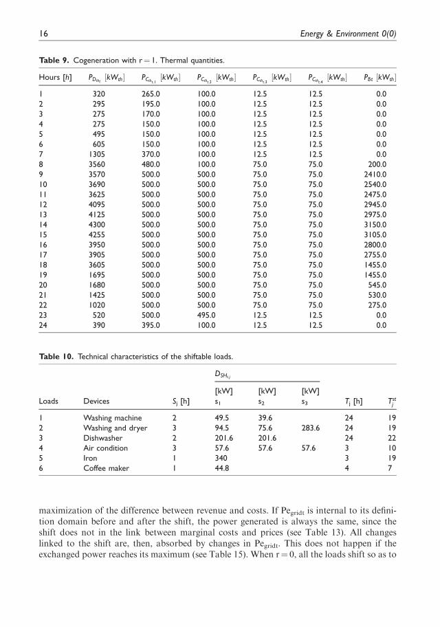
maximization of the difference between revenue and costs. If Pegridt is internal to its defini-tion domain before and after the shift, the power generated is always the same, since theshift does not in the link between marginal costs and prices (see Table 13). All changeslinked to the shift are, then, absorbed by changes in Pegridt. This does not happen if theexchanged power reaches its maximum (see Table 15). When r¼ 0, all the loads shift so as to
Table 9. Cogeneration with r¼ 1. Thermal quantities.
Hours [h] PDtht½kWth� PCtht;1 ½kWth� PCtht;2 ½kWth� PCtht;3 ½kWth� PCtht;4 ½kWth� PBt ½kWth�
1 320 265.0 100.0 12.5 12.5 0.0
2 295 195.0 100.0 12.5 12.5 0.0
3 275 170.0 100.0 12.5 12.5 0.0
4 275 150.0 100.0 12.5 12.5 0.0
5 495 150.0 100.0 12.5 12.5 0.0
6 605 150.0 100.0 12.5 12.5 0.0
7 1305 370.0 100.0 12.5 12.5 0.0
8 3560 480.0 100.0 75.0 75.0 200.0
9 3570 500.0 500.0 75.0 75.0 2410.0
10 3690 500.0 500.0 75.0 75.0 2540.0
11 3625 500.0 500.0 75.0 75.0 2475.0
12 4095 500.0 500.0 75.0 75.0 2945.0
13 4125 500.0 500.0 75.0 75.0 2975.0
14 4300 500.0 500.0 75.0 75.0 3150.0
15 4255 500.0 500.0 75.0 75.0 3105.0
16 3950 500.0 500.0 75.0 75.0 2800.0
17 3905 500.0 500.0 75.0 75.0 2755.0
18 3605 500.0 500.0 75.0 75.0 1455.0
19 1695 500.0 500.0 75.0 75.0 1455.0
20 1680 500.0 500.0 75.0 75.0 545.0
21 1425 500.0 500.0 75.0 75.0 530.0
22 1020 500.0 500.0 75.0 75.0 275.0
23 520 500.0 495.0 12.5 12.5 0.0
24 390 395.0 100.0 12.5 12.5 0.0
Table 10. Technical characteristics of the shiftable loads.
DSHt;j
[kW] [kW] [kW]
Loads Devices Sj [h] s1 s2 s3 Tj [h] Tstj
1 Washing machine 2 49.5 39.6 24 19
2 Washing and dryer 3 94.5 75.6 283.6 24 19
3 Dishwasher 2 201.6 201.6 24 22
4 Air condition 3 57.6 57.6 57.6 3 10
5 Iron 1 340 3 19
6 Coffee maker 1 44.8 4 7
16 Energy & Environment 0(0)

minimize the cost of electricity purchase; when r¼ 1, each load estimates if it is more con-
venient to shift in the intervals in which the cost is minimized or in the intervals in which the
revenue from the sale in reserve market is maximized. So, when r¼ 0, the load 4 (air
conditioners) shifts in the intervals 16–18 to which corresponds the minimum cost; when
r¼ 1, it does not shift because the revenue that is obtained if it stays where it is (equal to
2592) is bigger than the saving (equal to 2240) obtained if it would shift in 16–18 h.In addition to the mentioned case, it is also considered the case in which the probability is
not constant, assuming the value 0 or 1 depending of the interval Tables 16 and 17. Now
that, with the shift, intertemporal constraints were introduced, it makes sense to consider
that there are intervals in which rt is very high and in intervals in which it is very low.Let it show that load 4 shifts as the case 5.
Cogeneration and storage system
Finally, one only centralized electric storage unit, with a power rating of 500 kW and a
maximum stored energy of 4500 kWh, is assumed available. From a qualitative point of
view, nothing changes. The storage and the shift work in the same way, compatibly with
their respective different constraints (essentially, for the storage, the restoration of level and,
for the shift, Tj and Sj constraints).Table 18 reports the value of the daily management costs of the MG in all of cases that
were considered. The table reports the percentage variations of the total costs for cases 2–9
with respect to the case 1. The presence of storage leads to lower costs by bringing more
edibility to model. In absence of regulation, the arbitrage could be admitted. The arbitrage is
the simultaneous purchase and sale of energy to profit from a difference in the price. If it
happens, the units continue to be produced according to the marginal cost criteria, obtain-
ing the same previous results, but the amount of energy exchanged with the main grid Pegridtchanges. In fact, MG buys in the electricity market, for each hour, the maximum quantity of
energy admissible according to the constraints in order to sell the highest quantity of energy
into the reserve market. This, as shown in equation (1), requires that, in the model, the
powers PrGt;j and Pr
Cet;j P are limited from above by the difference between the maximum
power and the minimum power rather than the difference between the maximum power and
the power produced. In Table 19 are reported the results for some cases considered.
Table 11. Composition of the shiftable loads.
dSHt;j
Nj
[kW] [kW] [kW]
Loads Devices s1 s2 s3
1 Washing machine 0.5 0.4 99
2 Washing and dryer 0.5 0.4 1.2 189
3 Dishwasher 0.7 0.7 288
4 Air condition 0.2 0.2 0.2 288
5 Iron 1 340
6 Coffee maker 0.8 56
Ferruzzi et al. 17

Table
12.Cogenerationandshift
withr¼0.Shiftable
andshiftedloads.
Hours
[h]
Pe [e]
P DF t
[kW
e]
DSH
t;1
[kW
e]
DSH
t;2
[kW
e]
DSH
t;3
[kW
e]
DSH
t;4
[kW
e]
DSH
t;5
[kW
e]
DSH
t;6
[kW
e]
P DSH
t;1
[kW
e]
P DSH
t;2
[kW
e]
P DSH
t;3
[kW
e]
P DSH
t;4
[kW
e]
P DSH
t;5
[kW
e]
P DSH
t;6
[kW
e]
P0De t
[kW
e]
141.7
440.0
0.0
0.0
0.0
0.0
0.0
0.0
0.0
0.0
0.0
0.0
0.0
0.0
440.0
239.7
440.0
0.0
0.0
0.0
0.0
0.0
0.0
0.0
0.0
0.0
0.0
0.0
0.0
440.0
338.0
440.0
0.0
0.0
0.0
0.0
0.0
0.0
0.0
0.0
0.0
0.0
0.0
0.0
440.0
436.0
440.0
0.0
0.0
0.0
0.0
0.0
0.0
49.5
94.5
201.6
0.0
0.0
0.0
785.6
536.0
440.0
0.0
0.0
0.0
0.0
0.0
0.0
39.6
75.6
201.6
0.0
0.0
0.0
756.8
636.0
740.0
0.0
0.0
0.0
0.0
0.0
0.0
0.0
283.5
0.0
0.0
0.0
0.0
1023.5
739.8
1200.0
0.0
0.0
0.0
0.0
0.0
44.8
0.0
0.0
0.0
0.0
0.0
44.8
1200.0
844.6
1905.0
0.0
0.0
0.0
0.0
0.0
0.0
0.0
0.0
0.0
0.0
0.0
0.0
1905.0
949.5
2345.0
0.0
0.0
0.0
0.0
0.0
0.0
0.0
0.0
0.0
0.0
0.0
0.0
2345.0
10
51.8
2405.0
0.0
0.0
0.0
57.6
0.0
0.0
0.0
0.0
0.0
0.0
0.0
0.0
2357.4
11
46.3
2420.0
0.0
0.0
0.0
57.6
0.0
0.0
0.0
0.0
0.0
0.0
0.0
0.0
2362.4
12
40.8
2440.0
0.0
0.0
0.0
57.6
0.0
0.0
0.0
0.0
0.0
0.0
0.0
0.0
2382.4
13
39.3
2470.0
0.0
0.0
0.0
0.0
0.0
0.0
0.0
0.0
0.0
0.0
0.0
0.0
2470.0
14
38.5
2465.0
0.0
0.0
0.0
0.0
0.0
0.0
0.0
0.0
0.0
0.0
0.0
0.0
2465.0
15
43.7
2450.0
0.0
0.0
0.0
0.0
0.0
0.0
0.0
0.0
0.0
0.0
0.0
0.0
2450.0
16
42.0
2395.0
0.0
0.0
0.0
0.0
0.0
0.0
0.0
0.0
0.0
57.6
0.0
0.0
2452.6
17
44.9
2360.0
0.0
0.0
0.0
0.0
0.0
0.0
0.0
0.0
0.0
57.6
0.0
0.0
2417.6
18
48.3
2335.0
0.0
0.0
0.0
0.0
0.0
0.0
0.0
0.0
0.0
57.6
0.0
0.0
2392.6
19
44.5
1210.0
49.5
94.5
0.0
0.0
340.0
0.0
0.0
0.0
0.0
0.0
340.0
0.0
1551.0
20
45.0
1309.8
39.6
75.6
0.0
0.0
0.0
0.0
0.0
0.0
0.0
0.0
0.0
0.0
1309.8
21
55.0
1011.5
0.0
283.5
0.0
0.0
0.0
0.0
0.0
0.0
0.0
0.0
0.0
0.0
1011.5
22
59.4
753.4
0.0
0.0
201.6
0.0
0.0
0.0
0.0
0.0
0.0
0.0
0.0
0.0
753.4
23
55.0
328.4
0.0
0.0
201.6
0.0
0.0
0.0
0.0
0.0
0.0
0.0
0.0
0.0
328.4
24
50.7
425.0
0.0
0.0
0.0
0.0
0.0
0.0
0.0
0.0
0.0
0.0
0.0
0.0
425.0
18 Energy & Environment 0(0)

Table
13.Cogenerationandshift
withr¼0.Post
shift
state.
Hours
[h]
Pt Det
[kW
e]
Pe G1t
[kW
e]
Pe G2t
[kW
e]
Pe ce1t
[kW
e]
Pe ce2t
[kW
e]
Pe ce3t
[kW
e]
Pe ce4t
[kW
e]
Pe gridt
[kW
e]
P Dtht
[kW
th]
P Ce 1
tht
[kW
th]
P Ce 2
tht
[kW
th]
P Ce 3
tht
[kW
th]
P Ce 4
tht
[kW
th]
P Bt
[kW
th]
1440
180.0
180.0
212.0
80.0
10.0
10.0
�232.0
390.0
265.0
100.0
12.5
12.5
0.0
2440
180.0
180.0
156.0
80.0
10.0
10.0
�176.0
320.0
195.0
100.0
12.5
12.5
0.0
3440
180.0
180.0
136.0
80.0
10.0
10.0
�156.0
295.0
170.0
100.0
12.5
12.5
0.0
4440
180.0
180.0
120.0
80.0
10.0
10.0
205.6
275.0
150.0
100.0
12.5
12.5
0.0
5440
180.0
180.0
120.0
80.0
10.0
10.0
176.8
275.0
150.0
100.0
12.5
12.5
0.0
6740
180.0
180.0
296.0
80.0
10.0
10.0
267.5
495.0
370.0
100.0
12.5
12.5
0.0
71200
180.0
180.0
384.0
80.0
10.0
10.0
356.0
605.0
480.0
100.0
12.5
12.5
0.0
81905
180.0
180.0
400.0
400.0
60.0
60.0
625.0
1305.0
500.0
500.0
75.0
75.0
200.0
92345
180.0
180.0
400.0
400.0
60.0
60.0
1065.0
3560.0
500.0
500.0
75.0
75.0
2410.0
10
2405
180.0
180.0
400.0
400.0
60.0
60.0
1067.4
3570.0
500.0
500.0
75.0
75.0
2540.0
11
2420
180.0
180.0
400.0
400.0
60.0
60.0
1082.4
3690.0
500.0
500.0
75.0
75.0
2475.0
12
2440
180.0
180.0
400.0
400.0
60.0
60.0
1102.4
3625.0
500.0
500.0
75.0
75.0
2945.0
13
2470
180.0
180.0
400.0
400.0
60.0
60.0
1190.0
4095.0
500.0
500.0
75.0
75.0
2975.0
14
2465
180.0
180.0
400.0
400.0
60.0
60.0
1185.0
4125.0
500.0
500.0
75.0
75.0
3150.0
15
2450
180.0
180.0
400.0
400.0
60.0
60.0
1170.0
4300.0
500.0
500.0
75.0
75.0
3105.0
16
2395
180.0
180.0
400.0
400.0
60.0
60.0
1172.6
4255.0
500.0
500.0
75.0
75.0
2800.0
17
2360
180.0
180.0
400.0
400.0
60.0
60.0
1137.6
3950.0
500.0
500.0
75.0
75.0
2755.0
18
2335
180.0
180.0
400.0
400.0
60.0
60.0
1112.6
3905.0
500.0
500.0
75.0
75.0
1455.0
19
1695
180.0
180.0
400.0
400.0
60.0
60.0
271.0
3605.0
500.0
500.0
75.0
75.0
1455.0
20
1425
180.0
180.0
400.0
400.0
60.0
60.0
29.8
1695.0
500.0
500.0
75.0
75.0
545.0
21
1295
180.0
180.0
400.0
400.0
60.0
60.0
�268.5
1680.0
500.0
500.0
75.0
75.0
530.0
22
955
180.0
180.0
400.0
400.0
60.0
60.0
�526.6
1425.0
500.0
500.0
75.0
75.0
275.0
23
530
180.0
180.0
400.0
396.0
10.0
10.0
�847.6
1020.0
500.0
495.0
12.5
12.5
0.0
24
425
180.0
180.0
316.0
80.0
10.0
10.0
�351.0
520.0
395.0
100.0
12.5
12.5
0.0
Ferruzzi et al. 19

Table
14.Cogenerationandshift
withr¼1.Shiftable
andshiftedloads.
Hours
[h]
Pe½2�
P DF
[kW
e]
DSH
t;1
[kW
e]
DSH
t;2
[kW
e]
DSH
t;3
[kW
e]
DSH
t;4
[kW
e]
DSH
t;5
[kW
e]
DSH
t;6
[kW
e]
P De t
[kW
e]
P DSH
t;1
[kW
e]
P DSH
t;2
[kW
e]
P DSH
t;3
[kW
e]
P DSH
t;4
[kW
e]
P DSH
t;5
[kW
e]
P DSH
t;6
[kW
e]
P0De t
[kW
e]
141.7
440.0
0.0
0.0
0.0
0.0
0.0
0.0
440.0
0.0
0.0
0.0
0.0
0.0
0.0
440.0
239.7
440.0
0.0
0.0
0.0
0.0
0.0
0.0
440.0
0.0
0.0
0.0
0.0
0.0
0.0
440.0
338.0
440.0
0.0
0.0
0.0
0.0
0.0
0.0
440.0
0.0
0.0
0.0
0.0
0.0
0.0
440.0
436.0
440.0
0.0
0.0
0.0
0.0
0.0
0.0
440.0
49.5
94.5
201.6
0.0
0.0
0.0
785.6
536.0
440.0
0.0
0.0
0.0
0.0
0.0
0.0
440.0
39.6
75.6
201.6
0.0
0.0
0.0
756.8
636.0
740.0
0.0
0.0
0.0
0.0
0.0
0.0
740.0
0.0
283.5
0.0
0.0
0.0
0.0
1023.5
739.8
1152.2
0.0
0.0
0.0
0.0
0.0
44.8
1200.0
0.0
0.0
0.0
0.0
0.0
44.8
1200.0
844.6
1905.0
0.0
0.0
0.0
0.0
0.0
0.0
1905.0
0.0
0.0
0.0
0.0
0.0
0.0
1905.0
949.5
2345.0
0.0
0.0
0.0
0.0
0.0
0.0
2345.0
0.0
0.0
0.0
0.0
0.0
0.0
2345.0
10
51.8
2347.4
0.0
0.0
0.0
57.6
0.0
0.0
2405.0
0.0
0.0
0.0
0.0
0.0
0.0
2405.0
11
46.3
2362.4
0.0
0.0
0.0
57.6
0.0
0.0
2420.0
0.0
0.0
0.0
0.0
0.0
0.0
2420.0
12
40.8
2382.4
0.0
0.0
0.0
0.0
0.0
0.0
2440.0
0.0
0.0
0.0
0.0
0.0
0.0
2440.0
13
39.3
2470.0
0.0
0.0
0.0
0.0
0.0
0.0
2470.0
0.0
0.0
0.0
0.0
0.0
0.0
2470.0
14
38.5
2465.0
0.0
0.0
0.0
0.0
0.0
0.0
2465.0
0.0
0.0
0.0
0.0
0.0
0.0
2465.0
15
43.7
2450.0
0.0
0.0
0.0
0.0
0.0
0.0
2450.0
0.0
0.0
0.0
0.0
0.0
0.0
2450.0
16
42.0
2395.0
0.0
0.0
0.0
0.0
0.0
0.0
2395.0
0.0
0.0
0.0
57.6
0.0
0.0
2395.0
17
44.9
2360.0
0.0
0.0
0.0
0.0
0.0
0.0
2360.0
0.0
0.0
0.0
57.6
0.0
0.0
2360.0
18
48.3
2335.0
0.0
0.0
0.0
0.0
0.0
0.0
2335.0
0.0
0.0
0.0
57.6
0.0
0.0
2335.0
19
44.5
1211.0
49.5
94.5
0.0
0.0
340.0
0.0
1695.0
0.0
0.0
0.0
0.0
340.0
0.0
1551.0
20
45.0
1309.8
39.6
75.6
0.0
0.0
0.0
0.0
1425.0
0.0
0.0
0.0
0.0
0.0
0.0
1309.8
21
55.0
1011.5
0.0
283.5
0.0
0.0
0.0
0.0
1295.0
0.0
0.0
0.0
0.0
0.0
0.0
1011.5
22
59.4
753.4
0.0
0.0
201.6
0.0
0.0
0.0
955.0
0.0
0.0
0.0
0.0
0.0
0.0
753.4
23
55.0
328.4
0.0
0.0
201.6
0.0
0.0
0.0
530.0
0.0
0.0
0.0
0.0
0.0
0.0
328.4
24
50.7
425.0
0.0
0.0
0.0
0.0
0.0
0.0
425.0
0.0
0.0
0.0
0.0
0.0
0.0
425.0
20 Energy & Environment 0(0)

Table
15.Cogenerationandshift
withr¼1.Post
shift
state.
Hours
[h]
Pt Det
[kW
e]
Pe Gt;1
[kW
e]
Pe Gt;2
[kW
e]
Pe cet;1
[kW
e]
Pe cet;2
[kW
e]
Pe cet;3
[kW
e]
Pe cet;4
[kW
e]
Pe gridt
[kW
e]
Pr Gt;1
[kW
e]
Pr Gt;2
[kW
e]
Pr Ce t;1
[kW
e]
Pr Ce t;2
[kW
e]
Pr Ce t;3
[kW
e]
Pr Ce t;4
[kW
e]
Pr gridt
[kW
th]
P Dth
[kW
th]
P Ce th t;1
[kW
th]
P Ce th t;2
[kW
th]
P Ce th t;3
[kW
th]
1440.0
36.0
36.0
80.0
80.0
10.0
10.0
188.0
48.0
144.0
144.0
132.0
0.0
0.0
0.0
390.0
265.0
100.0
12.5
2440.0
36.0
36.0
80.0
80.0
10.0
10.0
188.0
45.0
144.0
144.0
76.0
0.0
0.0
0.0
320.0
195.0
100.0
12.5
3440.0
36.0
36.0
80.0
80.0
10.0
10.0
188.0
43.8
144.0
144.0
56.0
0.0
0.0
0.0
295.0
170.0
100.0
12.5
4785.6
36.0
36.0
80.0
80.0
10.0
10.0
533.6
41.4
144.0
144.0
40.0
0.0
0.0
0.0
275.0
150.0
100.0
12.5
5756.8
36.0
36.0
80.0
80.0
10.0
10.0
504.8
41.5
144.0
144.0
40.0
0.0
0.0
0.0
275.0
150.0
100.0
12.5
61023.5
36.0
36.0
80.0
80.0
10.0
10.0
771.5
41.4
144.0
144.0
216.0
0.0
0.0
0.0
495.0
370.0
100.0
12.5
71200.0
36.0
36.0
80.0
80.0
10.0
10.0
948.0
45.8
144.0
144.0
304.0
0.0
0.0
0.0
605.0
480.0
100.0
12.5
81905.0
36.0
145.0
400.0
213.0
10.0
10.0
1200.0
51.3
144.0
144.0
0.0
187.0
50.0
50.0
1350.0
500.0
500.0
75.0
92345.0
180.0
180.0
400.0
400.0
10.0
10.0
1200.0
56.9
0.0
0.0
0.0
35.0
50.0
135.0
3560.0
500.0
500.0
75.0
10
2405.0
180.0
180.0
400.0
400.0
35.0
10.0
1200.0
59.6
0.0
0.0
0.0
0.0
25.0
50.0
3690.0
500.0
500.0
75.0
11
2420.0
180.0
180.0
400.0
400.0
50.0
10.0
1200.0
53.3
0.0
0.0
0.0
0.0
10.0
50.0
3625.0
500.0
500.0
75.0
12
2440.0
180.0
180.0
400.0
400.0
50.0
20.0
1200.0
47.0
0.0
0.0
0.0
0.0
0.0
50.0
4095.0
500.0
500.0
75.0
13
2470.0
180.0
180.0
400.0
400.0
60.0
60.0
1200.0
45.2
0.0
0.0
0.0
0.0
0.0
10.0
4125.0
500.0
500.0
75.0
14
2465.0
180.0
180.0
400.0
400.0
60.0
35.0
1200.0
44.2
0.0
0.0
0.0
0.0
0.0
15.0
4300.0
500.0
500.0
75.0
15
2450.0
180.0
180.0
400.0
400.0
60.0
30.0
1200.0
50.2
0.0
0.0
0.0
0.0
0.0
30.0
4255.0
500.0
500.0
75.0
16
2395.0
180.0
180.0
400.0
400.0
25.0
10.0
1200.0
48.3
0.0
0.0
0.0
0.0
35.0
50.0
3950.0
500.0
500.0
75.0
17
2360.0
180.0
180.0
400.0
400.0
10.0
10.0
1200.0
51.6
0.0
20.0
0.0
20.0
50.0
50.0
3905.0
500.0
500.0
75.0
18
2335.0
180.0
135.0
400.0
400.0
10.0
60.0
1200.0
55.5
0.0
0.0
0.0
45.0
50.0
50.0
2605.0
500.0
500.0
75.0
19
1551.0
36.0
36.0
323.0
80.0
10.0
10.0
1056.0
51.2
144.0
144.0
77.0
320.0
50.0
50.0
2605.0
500.0
500.0
75.0
20
1309.8
36.0
36.0
80.0
80.0
10.0
10.0
1057.8
51.8
144.0
144.0
320.0
320.0
50.0
50.0
1695.0
500.0
500.0
75.0
21
1011.5
36.0
36.0
80.0
80.0
10.0
10.0
759.5
144.0
144.0
320.0
320.0
50.0
50.0
0.0
1680.0
500.0
500.0
75.0
22
753.4
36.0
36.0
80.0
80.0
10.0
10.0
501.4
68.3
144.0
144.0
320.0
320.0
50.0
50.0
1425.0
500.0
500.0
75.0
23
328.4
180.0
180.0
400.0
396.0
10.0
10.0
75.4
63.3
144.0
144.0
320.0
316.0
0.0
0.0
1020.0
500.0
495.0
12.5
24
425.0
36.0
36.0
80.0
80.0
10.0
10.0
173.0
58.3
144.0
144.0
236.0
0.0
0.0
0.0
520.0
395.0
100.0
12.5
Ferruzzi et al. 21

Table
16.Cogenerationandshift
withr¼0/1.Shiftable
andshiftedloads.
Hour
[h]
qe½e�
r t½%�
P DF
[kW
e]
DSH
t;1
[kW
e]
DSH
t;2
[kW
e]
DSH
t;3
[kW
e]
DSH
t;4
[kW
e]
DSH
t;5
[kW
e]
DSH
t;6
[kW
e]
P De t
[kW
e]
P DSH
t;1
[kW
e]
P DSH
t;2
[kW
e]
P DSH
t;3
[kW
e]
P DSH
t;4
[kW
e]
P DSH
t;5
[kW
e]
P DSH
t;6
[kW
e]
P0De t
[kW
e]
141.7
0.0
440.0
0.0
0.0
0.0
0.0
0.0
0.0
440.0
0.0
0.0
0.0
0.0
0.0
0.0
440.0
239.7
0.0
440.0
0.0
0.0
0.0
0.0
0.0
0.0
440.0
0.0
0.0
0.0
0.0
0.0
0.0
440.0
338
0.0
440.0
0.0
0.0
0.0
0.0
0.0
0.0
440.0
0.0
0.0
0.0
0.0
0.0
0.0
440.0
436
0.0
440.0
0.0
0.0
0.0
0.0
0.0
0.0
440.0
49.5
94.5
201.6
0.0
0.0
0.0
785.6
536
0.0
440.0
0.0
0.0
0.0
0.0
0.0
0.0
440.0
39.6
75.6
201.6
0.0
0.0
0.0
756.8
636
1.0
740.0
0.0
0.0
0.0
0.0
0.0
0.0
740.0
0.0
283.5
0.0
0.0
0.0
0.0
1023.5
739.8
1.0
1152.2
0.0
0.0
0.0
0.0
0.0
44.8
1200.0
0.0
0.0
0.0
0.0
0.0
0.0
1200.0
844.6
1.0
1905.0
0.0
0.0
0.0
0.0
0.0
0.0
1905.0
0.0
0.0
0.0
0.0
0.0
0.0
1905.0
949.5
1.0
2345.0
0.0
0.0
0.0
0.0
0.0
0.0
2345.0
0.0
0.0
0.0
0.0
0.0
0.0
2345.0
10
51.8
0.0
2347.4
0.0
0.0
0.0
57.6
0.0
0.0
2405.0
0.0
0.0
0.0
0.0
0.0
0.0
2405.0
11
46.3
0.0
2362.4
0.0
0.0
0.0
57.6
0.0
0.0
2420.0
0.0
0.0
0.0
0.0
0.0
0.0
2420.0
12
40.8
0.0
2382.4
0.0
0.0
0.0
57.6
0.0
0.0
2440.0
0.0
0.0
0.0
0.0
0.0
0.0
2440.0
13
39.3
0.0
2470.0
0.0
0.0
0.0
0.0
0.0
0.0
2470.0
0.0
0.0
0.0
0.0
0.0
0.0
2470.0
14
38.5
0.0
2465.0
0.0
0.0
0.0
0.0
0.0
0.0
2465.0
0.0
0.0
0.0
0.0
0.0
0.0
2465.0
15
43.7
1.0
2450.0
0.0
0.0
0.0
0.0
0.0
0.0
2450.0
0.0
0.0
0.0
0.0
0.0
0.0
2450.0
16
42
1.0
2395.0
0.0
0.0
0.0
0.0
0.0
0.0
2395.0
0.0
0.0
0.0
57.6
0.0
0.0
2395.0
17
44.9
1.0
2360.0
0.0
0.0
0.0
0.0
0.0
0.0
2360.0
0.0
0.0
0.0
57.6
0.0
0.0
2360.0
18
48.3
0.0
2335.0
0.0
0.0
0.0
0.0
0.0
0.0
2335.0
0.0
0.0
0.0
57.6
0.0
0.0
2335.0
19
44.5
0.0
1211.0
49.5
94.5
0.0
0.0
340.0
0.0
1695.0
0.0
0.0
0.0
0.0
340.0
0.0
1551.0
20
45
0.0
1309.8
39.6
75.6
0.0
0.0
0.0
0.0
1425.0
0.0
0.0
0.0
0.0
0.0
0.0
1309.8
21
55
0.0
1011.5
0.0
283.5
0.0
0.0
0.0
0.0
1295.0
0.0
0.0
0.0
0.0
0.0
0.0
1011.5
22
59.4
0.0
753.4
0.0
0.0
201.6
0.0
0.0
0.0
955.0
0.0
0.0
0.0
0.0
0.0
0.0
753.4
23
55
0.0
328.4
0.0
0.0
201.6
0.0
0.0
0.0
530.0
0.0
0.0
0.0
0.0
0.0
0.0
328.4
24
50.7
0.0
425.0
0.0
0.0
0.0
0.0
0.0
0.0
425.0
0.0
0.0
0.0
0.0
0.0
0.0
425.0
22 Energy & Environment 0(0)

Table
17.Cogenerationandshift
withr¼0/1.Post
shift
state.
Hour
[h]
P DF
[kW
e]
Pe Gt;1
[kW
e]
Pe Gt;2
[kW
e]
Pe cet;1
[kW
e]
Pe cet;2
[kW
e]
Pe cet;3
[kW
e]
Pe cet;4
[kW
e]
Pe gridt
[kW
e]
Pr Gt;1
[kW
e]
Pr Gt;2
[kW
e]
Pr Ce t;1
[kW
e]
Pr Ce t;2
[kW
e]
Pr Ce t;3
[kW
e]
Pr Ce t;4
[kW
e]
Pr gridt
[kW
e]
P Dtht
[kW
th]
P Ce tht;1
[kW
th]
P Ce th t;2
[kW
th]
P Ce th t;3
[kW
th]
1440.0
180.0
180.0
212.0
80.0
10.0
10.0
�232.0
0.0
0.0
0.0
0.0
0.0
0.0
390.0
265.0
100.0
12.5
2440.0
180.0
180.0
156.0
80.0
10.0
10.0
�176.0
0.0
0.0
0.0
0.0
0.0
0.0
320.0
195.0
100.0
12.5
3440.0
180.0
180.0
136.0
80.0
10.0
10.0
�156.0
0.0
0.0
0.0
0.0
0.0
0.0
295.0
170.0
100.0
12.5
4440.0
180.0
180.0
120.0
80.0
10.0
10.0
205.6
0.0
0.0
0.0
0.0
0.0
0.0
275.0
150.0
100.0
12.5
5440.0
180.0
180.0
120.0
80.0
10.0
10.0
176.8
0.0
0.0
0.0
0.0
0.0
0.0
275.0
150.0
100.0
12.5
6740.0
36.0
36.0
80.0
80.0
10.0
10.0
771.5
144.0
144.0
216.0
0.0
0.0
0.0
495.0
370.0
100.0
12.5
71152.2
36.0
36.0
80.0
80.0
10.0
10.0
948.0
144.0
144.0
304.0
0.0
0.0
0.0
605.0
480.0
100.0
12.5
81905.0
36.0
36.0
400.0
213.0
10.0
10.0
1200.0
144.0
144.0
0.0
187.0
50.0
50.0
1350.0
500.0
500.0
75.0
92345.0
180.0
145.0
400.0
400.0
10.0
10.0
1200.0
0.0
0.0
0.0
35.0
50.0
135.0
3560.0
500.0
500.0
75.0
10
2347.4
180.0
180.0
400.0
400.0
60.0
60.0
1067.4
0.0
0.0
0.0
0.0
0.0
0.0
3690.0
500.0
500.0
75.0
11
2362.4
180.0
180.0
400.0
400.0
60.0
60.0
1082.4
0.0
0.0
0.0
0.0
0.0
0.0
3625.0
500.0
500.0
75.0
12
2382.4
180.0
180.0
400.0
400.0
60.0
60.0
1102.4
0.0
0.0
0.0
0.0
0.0
0.0
4095.0
500.0
500.0
75.0
13
2470.0
180.0
180.0
400.0
400.0
60.0
60.0
1190.0
0.0
0.0
0.0
0.0
0.0
0.0
4125.0
500.0
500.0
75.0
14
2465.0
180.0
180.0
400.0
400.0
60.0
60.0
1185.0
0.0
0.0
0.0
0.0
0.0
0.0
4300.0
500.0
500.0
75.0
15
2450.0
180.0
180.0
400.0
400.0
60.0
30.0
1200.0
0.0
0.0
0.0
0.0
0.0
30.0
4255.0
500.0
500.0
75.0
16
2395.0
180.0
180.0
400.0
400.0
60.0
32.6
1200.0
0.0
0.0
0.0
0.0
0.0
32.6
3950.0
500.0
500.0
75.0
17
2360.0
180.0
180.0
400.0
400.0
47.6
10.0
1200.0
0.0
0.0
0.0
0.0
12.4
50.0
3905.0
500.0
500.0
75.0
18
2335.0
180.0
180.0
400.0
400.0
60.0
60.0
1112.6
0.0
0.0
0.0
0.0
0.0
0.0
2605.0
500.0
500.0
75.0
19
1211.0
180.0
180.0
400.0
400.0
60.0
60.0
271.0
0.0
0.0
0.0
0.0
0.0
0.0
2605.0
500.0
500.0
75.0
20
1309.8
180.0
180.0
400.0
400.0
60.0
60.0
29.8
0.0
0.0
0.0
0.0
0.0
0.0
1695.0
500.0
500.0
75.0
21
1011.5
180.0
180.0
400.0
400.0
60.0
60.0
�268.5
0.0
0.0
0.0
0.0
0.0
0.0
1680.0
500.0
500.0
75.0
22
753.4
180.0
180.0
400.0
400.0
60.0
60.0
�526.6
0.0
0.0
0.0
0.0
0.0
0.0
1425.0
500.0
500.0
75.0
23
328.4
180.0
180.0
400.0
396.0
10.0
10.0
�847.6
0.0
0.0
0.0
0.0
0.0
0.0
1020.0
500.0
495.0
12.5
24
425.0
180.0
180.0
316.0
80.0
10.0
10.0
�351.0
0.0
0.0
0.0
0.0
0.0
0.0
520.0
395.0
100.0
12.5
Ferruzzi et al. 23

Conclusions
The paper focused on the participation of an MG in both day-ahead energy and reservespinning market. It was shown how the MG solves a decision-making problem about thedevelopment of an optimal bidding strategy for both markets, evaluating different risktolerances (adverse, neutral, and incline).
An MG is considered in which both thermal and electrical loads must be satisfied, so thatin the MG only electricity power plants, CHP plants, and heat production plants (boilers)were already installed. The presence of thermal and electrical storage systems is alsoaccounted for. Moreover, it was considered that both generators and loads can take partin the reserve market. The demand participation happens through both shiftable and cur-tailable loads.
In this work the bidding strategy is limited to the submission, in the day-ahead electricitymarkets, of the only one value of the optimal hourly powers exchanged with the main grid,obtained in correspondence to the most probably hourly market profiles.
The paper showed the implementation of a new joint approach to take part in to the day-ahead market and spinning reserve market, formulated by a detailed mathematical optimi-zation model. It is written in the most general form as possible, allows to obtain the optimalvalues of power to offer in both markets that maximize the difference between revenues andcosts, in compliance with all existing technical and operational constraints. Numericalapplications of the approach are presented and discussed. The model was implementedfor different configurations. It was, first, supposed that all loads are fixed and that all thegeneration units (cogenerators and generators) produce only electricity, so that only a boilersatisfies the thermal load. In this configuration, cases were considered in which the proba-bility that the reserve is called to produce is very high (r¼ 1) or very low (r¼ 0). It was, then,considered the cogeneration, always assuming the presence only of fixed loads. Also in this
Table 18. Daily management costs—no arbitrage.
Case study OF [e] Boiler cost [e] Total cost [e] Variation (%)
Case_1 490.2 1735.8 2226.0
Case_2 324.2 1735.8 2060.0 �7.5
Case_3 1879.0 1879.0 �15.6
Case_4 1675.0 1675.0 �24.8
Case_5 1590.0 1590.0 �28.6
Case_6 1349.0 1349.0 �39.4
Case_7 1470.0 1470.0 �34.0
Case_8 1006.0 1006.0 �54.8
Case_9 870.0 870.0 �61.0
Table 19. Daily management costs with arbitrage.
Case study Total cost [e] Variation (%)
Case 2 1859.0 �9.8
Case 4 1430.0 �15.6
Case 6 1120.0 �18.3
Case 8 787.0 �21.8
24 Energy & Environment 0(0)

configuration, are considered the cases r¼ 1 and r¼ 1. Always considering the cogeneration,
it was supposed also that a percentage of the loads is shiftable. Now, in addition to cases
r¼ 1, it was also considered the case in which the probability is not constant, being able to
assume the value 0 or 1 depending on the interval. It is, finally, examined the case in which is
present a storage system. Everything presented and discussed clearly shows the effectiveness
of the model.Future research will focus on the formulation of the optimal bidding curves to present in
two markets and on the resolution of the Unit Commitment problem.
Declaration of conflicting interests
The author(s) declared no potential conflicts of interest with respect to the research, authorship, and/or
publication of this article.
Funding
The author(s) received no financial support for the research, authorship, and/or publication of
this article.
Note
a. The fixed load, for each interval, is curtailed by RES production.
References
1. Siano P, Graditi G, Atrigna M, et al. Designing and testing decision support and energy man-
agement systems for smart homes. J Ambient Intell Human Comput 2013; 4: 651–661.2. Silva M, Morais H and Vale Z. Distribution network short term scheduling in smart grid context.
In: Power and energy society general meeting, July 2011, pp.1–8. San Diego, USA: IEEE.3. Taheri H, Rahimi-Kian A, Ghasemi H, et al. Optimal operation of a virtual power plant with risk
management. Washington, DC, USA: Innovative Smart Grid Technologies (ISGT), 2012.4. Rossi F. Gestione dei sistemi elettrici nei mercati liberalizzati. Napoli, Italy: Edizioni Scientifiche
Italiane (ESI), 2007.5. Franco E, Lobato L, Rouco A, et al. Optimization of the spanish market sequence by a price-taker
generating firm. In: Power Tech conference proceedings, Vol. 2, 2003, p.6.6. Kuznetsova E, Li Y, Ruiz C, et al. An integrated framework of agent-based modelling and robust
optimization for microgrid energy management. Appl Energy 2014; 129: 70–88.7. Wang Q, Zhang C, Ding Y, et al. Review of real-time electricity markets for integrating distributed
energy resources and demand response. Appl Energy 2015; 138: 695–706.8. Swider D. Efficient scoring-rule in multipart procurement auctions for power systems reserve.
IEEE Trans Power Syst 2007; 22: 1717–1725.9. Pablo G, Jose V, Cristian AD, et al. Joint energy and reserve markets: current implementations
and modeling trends. Electr Power Syst Res 2014; 109: 101–111.10. Singh H and Papalexopoulos A. Competitive procurement of ancillary services by an independent
system operator. IEEE Trans Power Syst 1999; 14: 498–504.11. Yao M, Hu Z, Stufentes F, et al. Integrated power management of conventional units and indus-
trial loads in China’s ancillary services scheduling. Energies 2015; 8: 3955–3977.12. Ferruzzi G, Rossi F and Russo A. Determination of the prosumers optimal bids. Int J Emerg
Electr Power Syst 2015; 16: 537–548.
Ferruzzi et al. 25
13. Raineri R, Ros S and Schiele D. Technical and economic aspects of ancillary services markets inthe electric power industry: an international comparison. Energy Policy 2006; 34: 1540–1555.
14. Rebours Y, Kirschen D, Trotignon M, et al. A survey of frequency and voltage control ancillaryservices – part II: economic features. IEEE Trans Power Syst 2007; 22: 358–366.
15. Nezamabadi H and Nazar M. Arbitrage strategy of virtual power plants in energy, spinningreserve and reactive power markets. IET Gen Transm Distrib 2016; 10: 750–763.
16. Bai H, Miao S, Ran X, et al. Optimal dispatch strategy of a virtual power plant containing batteryswitch stations in a unified electricity market. Energies 2015; 8: 2268–2289.
17. Chitkara P, Zhong J and Bhattacharya K. Oligopolistic competition of gencos in reactive powerancillary service provisions. IEEE Trans Power Syst 2009; 24: 1256–1265.
18. Jia X, Zhou M and Li G. Study on conjectural variation based bidding strategy in spinning reservemarkets. In: International conference on Power System Technology (PowerCon 2006), 2006,pp.1–5.
19. Wang J, Wang X and Wu Y. Operating reserve model in the power market. IEEE Trans Power
Syst 2005; 20: 223–229.20. Ugedo e, Lobato A, Franco L, et al. Strategic bidding in sequential electricity markets. IEE Proc
Gen Transm Distrib 2006; 153: 431–442.21. Campos F, Munoz San Roque A, Sanchez-Ubeda E, et al. Strategic bidding in secondary reserve
markets. IEEE Trans Power Syst 2016; 31(4).22. Allen EH and Ilic MD. Reserve markets for power systems reliability. IEEE Trans Power Syst
2000; 15: 228–233.23. Attaviriyanupap H, Kita H, Tanaka E, et al. A new profit-based unit commitment considering
power and reserve generating. In: Power Engineering Society Winter Meeting, 2002. Vol. 2, 2002,pp.1311–1316. NY, USA: IEEE.
24. Attaviriyanupap P, Kita H, Tanaka F, et al. New bidding strategy formulation for day-aheadenergy and reserve markets based on evolutionary programming. Int J Electr Power Energy Syst
2005; 27: 157–167.25. Wen F and David A. Optimally coordinated bidding strategies in energy and ancillary service
markets. IEE Proc Gen Transm Distrib 2002; 149: 331–338.26. Wen F and David A. Coordination of bidding strategies in day-ahead Energy and spinning reserve
markets. Int J Electr Power Energy Syst 2002; 24: 251–261.27. Rajabi Mashhadi H and Khorasani J. Price-takers bidding strategies in joint energy and spinning
reserve pay-as-bid markets. Iran J Electr Electron Eng 2013; 9: 36–43.28. Yamin H. Spinning reserve uncertainty in day-ahead competitive electricity markets for gencos.
IEEE Trans Power Syst 2005; 20: 521–523.29. Mashhour E and Moghaddas-Tafreshi S. Bidding strategy of virtual power plant for participating
in energy and spinning reserve markets. Part I: problem formulation. IEEE Trans Power Syst
2011; 26: 949–956.30. Shi L, Luo Y and Tu G. Bidding strategy of microgrid with consideration of uncertainty for
participating in power market. Int J Electr Power Energy Syst 2014; 59: 1–13.31. Narimani I and Goldani S. Participating of micro-grids in energy and spinning reserve markets
intra-day market. Int J Smart Electr Eng 2015; 4: 19–21.32. Dabbagh SR and Sheikh-El-Eslami MK. Risk assessment of virtual power plants offering in
energy and reserve markets. IEEE Trans Power Syst 2016; 31: 3572–3582.33. Ferruzzi G, Graditi G, Rossi F, et al. Optimal operation of a residential microgrid: the role of
demand side management. Intell Ind Syst 2015; 1: 61–82.34. Zamani AG, Zakariazadeh A and Jadid S. Day-ahead resource scheduling of a renewable energy
based virtual power plant. Appl Energy 2016; 169: 324–340.35. Wei W, et al. Robust energy and reserve dispatch under variable renewable generation. IEEE
Trans Smart Grid 2014; 6: 369–380.
26 Energy & Environment 0(0)

36. Tabar VS, Jirdehi MA and Hemmati R. Energy management in microgrid based on the multi
objective stochastic programming incorporating portable renewable energy resource as demand
response option. Energy 2017; 118: 827–839.37. Gupta R and Gupta NK. A robust optimization based approach for microgrid operation in
deregulated environment. Energy Convers Manage 2015; 93: 121–131.38. Dimeas AL and Hatziargyriou ND. Operation of a multiagent system for microgrid control. IEEE
Trans Power Syst 2005; 20: 1447–1455.39. Liua L, et al. Energy management of cooperative microgrids: a distributed optimization approach.
Electr Power Energy Syst 2018; 96: 335–346.
Gabriella Ferruzzi received the Ph.D. in Science and Technology Management at the
University of Naples, Federico II, in 2013. She is currently researcher with the
Department of Industrial Engineering at University of Naples where she teaches courses
on General and Management Accounting and Energy Economics. Research interest focus
on the application of SmartGrid to utility systems and economical issues which arise from
the deregulated energy market. This work includes MicroGrids, Demand Side Management,
Distributed Generation, Energy Policies, Renewable energy sources. She is a Fellow of
IEEE and of AIEE.
Giorgio Graditi received the M.S and Ph.D. degrees in electrical engineering from the
University of Palermo, Palermo, Italy, in 1999 and 2005, respectively. Since 2011, he has
been the head of PV Systems and Smart Grid Unit, ENEA, Portici, Italy. In 2017, he
received the Italian accreditation as Full Professor of Electrical Energy Engineering. He
has co-authored more than 200 papers including more than 60 international journal papers.
He is the coordinator of National and European projects on RES and smart grid. His
research interests include power systems design and control, PV, smart grids modeling
and analysis, and multiobjective optimization applications.
Federico Rossi received the M.S and Ph.D. degrees in electrical engineering from the
University of Naples, Italy, in 1972 and 1975, respectively. He had his first university teach-
ing assignment in 1976, after being a post-doctoral researcher at Rice University in Houston
(Texas), USA.
Associate professor at the Faculty of Engineering of the University of Naples and then an
ordinary professor at the University of Salerno and University of Cassino, he was professor
of Energy Systems Management at the Faculty of Engineering at the University of Naples
Federico II, from 1 November 2004 until. In his scientific activity he initially carried out
studies concerning the planning and optimal management of large electrical systems and
general problems on energy policies.
Appendix
Notation
CBjðÞ production cost of the jth boiler
CcjðÞ production cost of the jth cogeneration unitCDCUj
ðÞ curtailment cost of the jth load
Ferruzzi et al. 27

CGjðÞ production cost of the jth generation unit
DSHt;jshiftable power of the jth load
E (x) expected value of generic quantity “x”Ksj charge/discharge thermal efficiency coefficientPBt;j
thermal power of the jth boilerPeCet;j
electric power of the jth CHP unit for the energy marketPrCet;j
electric power of the jth CHP unit for the spinning reserve marketPeDcut;j
power curtailable of the jth load for energy marketPrDcut;j
power curtailable of the jth load for spinning reserve marketPDFt;j
power of the jth electrical fixed load reduced by the amount of electricRES forecasted
PDSHt;jshifted power of the jth load
PDtht;j power of the jth thermal fixed load reduced by the amount of electricRES forecasted
Pegridt
power interchanged with the MV grid for the energy marketPrgridt
power interchanged with the MV grid for the reserve marketPeGt;j
power of the jth unit for the energy marketPrGt;j
power of the jth unit for the spinning reserve marketPSEt;j
power of the jth electrical storage unitPSTt;j
power of the jth thermal storage unitrt perceived probability the reserve is called (or not)st hourly interval of Sj
Sj cycle duration of the jth shiftable loadTj time window of the jth shiftable loadTstj time at which the jth shiftable loads starts
ut;j binary variablesWSEt;j
level of the jth electrical storage unitWSTt;j
level of the jth thermal storage unitaj economic coefficient of second order of the j-ma power plantsb economic coefficient of first order of the j-ma power plantscc economic constant coefficientgj cogeneration rationqet energy market priceqrt spinning reserve market priceXB set of boilersXC set of cogeneration power plants (CHP)
XDCUset of curtailable electrical loads
XDFset of fixed electricity loads
XDSEset of electricity storage units
XDSHset of shiftable electrical loads
XDSTset of thermal storage units
XDthset of thermal loads
XG set of power production plants
28 Energy & Environment 0(0)


![Optimal Bidding Strategy for Renewable Microgrid with ... · controllable resource. The bidding strategies proposed in [7–11] do not however consider network conditions and physical](https://img.pdfslide.net/doc/110x75/5ec6ed6e323d3309ae03bee7/optimal-bidding-strategy-for-renewable-microgrid-with-controllable-resource.jpg)


![Joint Investment and Operation of Microgrid · 2015-11-09 · and microgrid operation. While in [9]–[12], only microgrid operation is studied under given microgrid facilities. However,](https://img.pdfslide.net/doc/110x75/5f055ca67e708231d412960b/joint-investment-and-operation-of-microgrid-2015-11-09-and-microgrid-operation.jpg)