Embed Size (px)
Citation preview
1
A Kummer function based Zeta function theory to prove the Riemann Hypothesis
Dr. Klaus Braun January 31, 2017
Summary
Let H and M denote the Hilbert and the Mellin transform operators. For the Gaussian function )(xf it holds
)2
(2
1)( 2/ s
sfM s , )
2(
2
1)
2(
2)()( 2/2/ sss
sxfxM ss .
The corresponding entire Zeta function is given by ([EdH] 1.8)
)1()()()()1()()1)(2
(2
:)( 2/ ssxfxMssssss
s s .
The central idea is to replace
)()()()( sxfMsxfxM H
with )(:)( xfHxfH , 0)0(ˆ Hf and
)2
tan()2
()(),2
3,1(2)()( 2
1
2
11 ss
sxFxMsxfM
s
H
.
This enables the definition of an alternative entire Zeta function in the form (§2)
)()2
tan()2
()1(:)( 2
1
* sss
ss
s
.
with same zeros as )(s . It enables a modified formula for )(xJ ([EdH] 1.13 ff.).
The fractional part function
)1,0(2sin
2
1::)( #
2
1
Lx
xxxx
is linked to the Zeta function by ([TiE] (2.1.5), lemma 2.1)
)1()()1()1()1( sxxMsMss .
The Hilbert transform of the fractional part function is given by
)1,0()sin(2log12cos
)( #
2
1
Lxx
xH
, 0)0(ˆ H , #
1 HH .
Applying the idea of above leads to the replacement (§3)
)1()1()( ssxxM )1()( sxM H
s
ss
sss
xMsxM H
)()()
2()
2
1(2)1()
2cos)1()( 1
1
with same zeros as )1( s .
The integral function representations of the Zeta functions above based on the Hilbert
transforms of the Gaussian and the fractional part functions enable all “convolution”
related Polya-RH criteria ([CaD]), e.g. the Hilbert-Polya conjecture, Polya polynomial
criteria ([EdH] 12.5), as the Hilbert transform is defined by a singular (convolution)
integral operator.
The #
1H Hilbert space is the same as applied in [BaB] to reformulate the Beurling-
Nyman criterion. The non-vanishing constant Fourier term of the series causes same
“self-adjoint integral operator” building issue than in case of the Gaussian function.
2
The related entire Riemann function enables the definition of correspondingly defined
alternative Keiper-Li coefficients ([LaG]). It is enabled by the zeros of the concerned
Kummer functions and the related zeros of the Hilbert transformed Hermite polynomials.
The challenging part to verify the RH (prime number counting error function) criterion
)()log()()( 2
1
xOxxOxlix
is the asymptotical behavior of the exponential (integral) function ([EdH] 1.14 ff.)
x t
x
y
x
y dtt
e
y
dyeydexEi log:)(
given by Ramanujan’s asymptotic power series ([BeB] IV)
0
12
12 !)1()(
2
kk
kx
x
k
x
exEi .
The non-normalized (exponential) error function is given by ([AbM] 13.6)
0
12
012!
)1(:)(
2
k
kkx
t
k
x
kdtexerf .
Its relationship to the Kummer functions is given by ([AbM] 7.15)
),2
3,1(),
2
3,
2
1()( 2
11
2
1
2
xFxexxFxerf x.
The asymptotics of the corresponding non-normalized )(xerfc function is given by
(lemma D4, [OlF] chapter 3, 1.1; chapter 12 1.1, ([AbM] 7.1.23)
01212
)12....(31)1()(1)(
2
kkk
kx
x
kexerfxerfc .
It further holds ([LeN] 9.13)
),
2
3,1(2
2
1),
2
1,
2
1(
2
1),
2
3,1(
2
1)( 2
11
22 2222
xFxeexexexerfc xxxx
i.e.
),2
3,
2
1(
2),
2
3,1(
2)( 2
11
2
1
2
xFxxFexxerfc x .
The above relationships provide the linkage of the concerned Kummer functions with the
RH ( )(xli function) convergence criterion.
We further note the following properties:
i) the function represented by
012)12(
)1(
kk
k
xk
, 1x .
has the value 2/ as 0x , 0x ([BeB] IV, (10.2))
ii) )(22
xFeH x ,
1 )2(
)12...(311
1)(2
kk
x
x
k
xx
xF
x
eH
, ([GaW])
iii) 1
0
)
)2
sin(
1()12(
)1(
ps
ks
k
p
s
k
for 1)Re( s ([BeB] 5, Corollary 4)
implying the convergence of the series
p
pp )2
sin(1 .
3
We also note the following properties of the concerned hypergeometric functions ([AbM]
p.507, [OlF] p. 44/67).
0
11!12
)1(),
2
3;
2
1(
n
nn
n
x
nxF
and ),2
3;1(11 xF .
They are related to the error function and the Dawson function by
0
12
!12
)1(2)(
n
nn
n
x
nxerf
and
x
xtx ixerfei
dteexF0
)(2
)(222 .
The corresponding Mellin transforms (valid in the critical stripe) are given by
)2
(1
1),
2
3;
2
1(
0
11
2/ s
sx
dxxFx s
,
)2
sin()(),2
3;1(
2
1
0
11
2/ ssx
dxxFxs
.
The function
),2
3;
2
1(11 zF
has only imaginary zeros n fulfilling ([SeA], [SeA1], Note O5/38/39)
nanann
n
n
n
2
)Im(:
2
1
2
)Im(:1 212
.
Remark: Taking the logarithmic derivative of the Riemann functional equation one gets
([IvA] (12.21))
)2
tan(2)1(
)1(
)(
)(
)(
)()2log( s
s
s
s
s
s
s
Putting
)1(
1)
2sin(2
)2
cos()(2
)2(:)( 1
ss
ss
s sss
it holds on the critical line ([IvA] 4.3)
)(log
)2
1(
)2
1(
)2log( 2
tOt
it
it
.
Remark: On the critical line it holds ([AbM] 4.1.15)
)logsin()logcos(
)logsin()logcos(
)2
sin()2
cos(
)2
sin()2
cos(
)2
sinh()2
cosh(
)2
sinh()2
cosh(
))2
1(
2tan()
2tan(
itit
itit
ti
ti
ti
ti
tit
tit
its
resp.
)2
1()
2
1(
)sin())
2(tan(glo
2itit
ss
.
Remark: Let )(sL denote a Dirichlet function, then )(log sL is regular for 2/1 .
4
The analog approach based on the fractional part function
There is an analog approach to the Gaussian function above with respect to the fractional part function )(x and its relationship to the function by the equality
)1()()()1()( ssssxM .
It corresponds to the isomorphism of
2),( lH .
We note that the function )()( xHxH has mean value zero, i.e the norm below is defined
and the prerequisites of the theorems in Note S36 are fulfilled.
The function )(xH has a convergent Fourier series representation in a weak )1,0(#
1H
sense, which is equivalent to the )cot( x function, i.e.
)1,0()()2sin(2)cot( #
1
1
Hxxx H .
This generalized Fourier series representation of )cot( x is Cesàro summable (mean of
order one) ([ZyA] VI-3, VII-1). It leads to a function representation in the form
)()2
cot()()2
cos()1()1()2()1()cot()1()( 1 sssssssxMsxM s
H
.
With respect to a corresponding Dirchlet series representation we note that ([TiE] 4.14)
z
dzzz
in
ix
ix
s
xns
)cot((2
11 1
.
We further note (see also Notes S32/33) that
nn
S
vnuidguvuS1
),(
defines an inner product on *2/1
2
2/1
2 )( ll ([NaS]), i.e. the generalized Fourier coefficients
nun are square summable.
For functions with vanishing constant Fourier term (i.e. with zero mean, where the
Hilbert transform defines a unitary mapping, see also Note S36) the norm of the
corresponding dual space is given by
1
22
2/1
1nu
nu .
The Hilbert space 2/1
2
l is part of the Hilbert scale
2l whereby it holds
2/12/1),(
vuvu .
Especially one gets for 1
2
lu , 2
0
2 llv
012/1),( vuvu
.
The distributional Hilbert spaces 2l ( 1,2/1,0 ) play a key role
- in [BrK3] in order to define an alternative new ground state energy for the
harmonic quantum oscillator (see also Note O52 for the Weyl-berry conjecture)
- in [BrK1] providing a global, unique solution of the non-stationary, non-linear 3D-
Navier-Stokes equations
- in [BaB] (see also [BrK2]) where a functional analysis reformulation of the Nyman
criterion is provided (see below).
5
The Dirichlet series (see also Notes S44/45/47) on the critical line
1
log:)( ns
neasf
1
log:)( ns
nebsg
are linked to the Hilbert space 2/1
2
#
2/1
lH by ([LaE] §227, Satz 40):
1
2/1
1)2/1()2/1(
2
1lim:, nnba
ndtitgitfgf
.
As it holds ([EdH] 9.8)
log)(2
1 2dtt
one gets (see also Notes S32/33)
T
T nT n
dttT 1
22
2/1)1(
1)(
2
1lim
, 1
12
1
0
2
12
2
1
)(
1
log
6)2(
1
nn n
ndx
x
x
n
.
From Remark 2.8 below we recall the identity
2
1
)cosh(2
1)2/1(
2
1:)(
2
1 22
t
dtdtitdtt
, i.e. 2/1
2
l .
Theorem (Bagchi-Nyman criterion, [BaB]): Let
,....3,2,1)(: nk
nk
for ,...3,2,1k
and k be the closed linear span of k . Then the Nyman criterion states that the
following statements are equivalent:
The Riemann Hypothesis is true k .
Alternatively to the double infinite matrix k above we propose the analog defined double
infinite matrix
,....3,2,1)/(: nknH
H
k for ,...3,2,1k .
For any 1
2
lu , 2
0
2 llv , as it holds
012/1),( vuvu
,
the inner product 2/1),( vu is defined.
Putting
1
2:~ lu ,
2))sin(2log(:~ Ldv
this leads to the representation
),(),(),(),(),(),( 02/12/12/1 HHHHk SSd .
As 2/1
2
l is dense in 1
2
l with respect to the 1
2l norm, belongs to the closed linear span of
Nk
H
k , i.e.
1
2/1
2
1
2
ll
which fulfills the Bagchi criterion.
6
The analog approach related to the von Mangoldt density function )(x
We propose the Landau density function )(x alternatively to the Riemann density
function )(xJ and the von Mangoldt function )(x . They are related by
xdJdxd log .
With respect to the scope of [KoJ], [ViJ] we note the asymptotics
1)(
lim)log()()(lim1
x
x
n
xn
dx
dx
n
.
The alternative approach leads to th alternative asymptotics in the form
1)(
lim x
x
x
)2log(
log
)(lim
x
x
The Riemann and von Mangoldt densities are related to the Zeta function by (see also
notes S19/30/41, O19/20/21)
00
1 )()()(log xdJxdxxJxss ss
00000
1 )()()(log)()(
)()(glo xdxsxdJxxxdxdxx
xxsdxxxss sssss
.
It holds ([LaE] §50, [ScW] IV, ([PrK] III §3, Note S39)
xs
dsx
ss
s
innxx
n
xnx s
n
i
i
1
2
21 )(
)(
2
1)log()(log)()log()()(
resp. with ([PrK] VII §4, Note S50)
)2log()0(
)0(:
c ,
2
2
12
2 1log
2
1)
11log(
2
1
2
1
x
x
xx
nn
n
, 12 x
)1()2(
log)(
)(2
2
2
0
n
nx
n
xxxcxdt
t
tx
)1()2(
12)
11log(
2
1log)( 2
222
n
n
xn
n
x
xxcxx
)1
1log(2
1)2lg()0()0(
2
1:)(
20x
xxxxx
.
The Landau density function )(x is linked to the Zeta function by ([OsH] Bd. 1, 8, [KoJ],
Note O51)
(*)
0000
1 )(log)(:)()()(
)()(gloxdTxxdTexdxdxxxs
ss
s
s
s ssxss
, its , 0 .
The proof of (*) applies the fundamental identity ([LaE] §48, [ScW] IV, ([PrK] III §6)
10
1
0
log
2
12
2y
yy
s
ds
s
y
i
i
i
s
.
With respect to corresponding convergent Dirchlet series representation we refer to [LaE]
Bd. 2, theorem 51, Note S47.
Remark: We note the “regularity” relationship between the above three density functions
(in a weak “Hilbert scale” framework) given by
2/12/1 HHH
)()()( xxxJ .
7
Remark ([OsH] Bd. I, §8, Note O51): As )()( xexT is monotone increasing, and
0 0
)(log)()(glo
:)( xdTxxdTes
ssf ssx , its , 0
convergent. Then, as
)2log()0(
)0(
)(
)(lim)(lim
00
s
sssf
ss
exists, this holds also for
x
xT
x
)(lim
and both limits are identical, i.e.
)2log(log
)(lim
log
)(loglim
)(lim)(lim
0
x
x
x
xT
x
xTssf
xxxs
.
Remark: Von Mangoldt proved the Euler conjecture, i.e. that ([PrK] III, §5)
0...6
1
5
1
3
1
2
11
)(
1
n n
n .
The convergence of this series is a consequence of the PNT.
The convergence of ([PrK] III, §5)
(**) 1
log)(
1
n n
nn i.e. 1)
1log(
)(
1
nn
n
n
was proven by E. Landau ([LaE] §150). It cannot be derived from the PNT. In this
context we recall the corresponding comment from E. Landau concerning his proof ([LaE]
§159)
“… (it) goes deeper than the prime number theorem ...” .
The Landau theorem (**) can be represented in the following form ([TiE] 7.1, 7.9)
dtitvituvubann
nn
nn
n
)2/1()2/1(2
1lim:,:
1)
1log()(
11 2/1
11
i.e. the 2/1H inner product of the related functions exists,
i.e.
1
2/1
)(:)
2
1(
ns
Hn
nitu
, 2/1
1
)/1log(:)
2
1(
Hn
nitv
ns
.
From [PrK] III, §5, we recall for 1
1
)(
)(
1
nsn
n
s
,
1
11)(
nsnns
s
i.e.
11
11)(
)(
)(
ns
ns nnn
n
ss
s
.
Remark: If the RH is true, it holds ([LaE] LXXXI)
i)
1
)(
nsn
n is convergent for ...82.0222
ii)
pn
nspn
ssZ,
1)(log)(
is regular for .0,2/1 t
8
Remark: We note that for
)(log1
:)(log~
n
x
nxT
xn
, 1x
the inverse mapping is given by ([ScW] lemma 3.3)
)(log)(
)(log~
:)( 1
n
x
n
nxTx
xn
.
With
)log()log()1
(log)log(n
y
n
x
nn
xy
it follows
)()(log)()( yxnnxy
)()(1)( yxxy .
Remark: The asymptotics of the Riemann, the von Mangoldt and the Landau functions
are given by
x
x
n
nxJ
xn loglog
)()(
, xnxxn
)()( , xn
xnx
xn
)log()()( .
The asymptotics xx )( leads to the PNT, whereby the convergence of the summand
x
requires special attention ([EdH] 4.1, [LaE] §89), i.e.
xx )( iff 0lim
1
x
x
.
Remark: The relative error in )()( xLix goes to zero faster than 2/1x as x is
equivalent to the RH ([EdH] 5.1).
Remark: In [ViJ] a quick distributional way to the Prime Number Theorem (PNT) is
provided. In this context we note that the regularity of the applied Dirac function is given
by
2/1, HH
where
)(glo1
)(n
x
xxH
and (in a distributional sense)
xn
nxnx )()()( ,
xn
nxHnx )()()( .
For the relationship to the )cot( x function we refer to [EsR] example 78, and to
the appendix section “Cardinal series”.
Putting )2log()0(/)0( c one gets from the PNT
1)(
x
x resp. xcx
x
xc
x
xc
xx
cx
x
log
)(
/1
)(
/1
/)()(
where
)1()2(
12)
11log(
2
1log)( 2
222
n
n
xn
n
x
xxcxx
.
9
Remark: The above provides alternatives in the form
xcx
x
cx
x
x
x
x
xx
log
)()()(log)(
cx
xx
x
xxcx
x
1
2
21
log
)(
)1
1log(2
1log
)( .
resp. x
x
x
x
x
xx
log
)(
log
)()(
x
x
x
x
x
xx
x
xxlix
1log
)(
))2log(1
1log(
log
11
1
log
)()((
2
*
The Riemann Hypothesis states that
0)( s for all its with 12/1 ,
i.e.
)(
)(,
)(
1
ss
s
s
has no poles in case of 12/1 .
We note the following equivalent critera for the RH:
i) )log()()( xxOxLix
ii) )()()( 2/1 xOxLix , 0 , ( 2/1
*
2/1( HH )
iii) )log()( 2 xxOxx
iv) The series s
n
nn
1
)( is convergent for 2/1)Re( s and
1
)(
)(
1
nsn
n
s
.
Remarks: iv) states that
)(
1
s
is holomorphic for 2/1)Re( s ; from ii) one can derive that
ss
s
1
1
)(
)(
is holomorphic for 2/1)Re( s ;
von Mangoldt’s explicit formula regarding )(x is given by
c
x
xx
Nx
Nx
xx
x
x )1
1log(2
1
)(2
1)
2
11(
)(
:)(20
, 84.1)2log(
)0(
)0(:
c
.
The proof that iii) is valid in case the RH is true, is based on the estimate
T T
xxO
xxx
,
2
)log
()( for xT 2 .
Putting xT with 4x this leads to
x T
xxOxOxx
,
2
)log
()1
()( .
10
Because of
)(log)1()log
(1 2
,,
xOOn
nO
xx
and ([GrI] 0.131, 0.133)
n
k k
k
knnn
A
nn
k1 2 )1)...(1(2
1log
1
(note
2
2 4
3
1
1
k k
).
one gets
)log()( 2 xxOxx .
With respect to the below we note
xxx
,,
2
,
21
1
1
11 .
Combining von Mangoldt’s formula with the Landau function leads to
)1()2(
12)1()log1(2)()( 2
20
n
n
xn
nxxcxxx
cxn
nx
xxcxx n
n
1)2(
12)1()
11log(log)()( 2
220
where
)2log(1 eec .
Proposal: We propose an alternative Li-function in the form
x
xx
log
)()(
x
xx
xx
xxcx
log2
)()(
)()(
)()(
2)( 0
0
0
.
For the Zeta function and
1
)(
)(
1
nsn
n
s
,
1
11)(
nsnns
s
we capture some related (mean value) H norm estimates on the critical line 2/1 :
1
2
2/1)1(
1
n n ,
1
12
12
2
1
)()2(
1
nn n
n
n
12/1
)(1,
)(
1
n n
n
s
,
12/1
log)(
)(,)(
1
n
nn
nsv
s
,
12
2/1
)()(,
)(
1
n n
n
s
s
s
.
Remark: A related 1
2l identity is given by ([ApT] 3.12)
)log
()(log6log)()(
21
22 x
xOx
n
nn
n
n
nxn
.
11
Remark: In the critical strip the Zeta function is a function of finite order in the sense of
the theory of Dirchlet series ([TiE] V). In particular it holds
)164/27
4/1
4/1
(
)log(
)(
)2
1(
tO
ttO
tO
it
))log(log
log(
)1(
1),1(glo),1(
t
tO
ititit
.
For the auxiliary function )(s it holds ([TiE] 4.12, [IvA] 4.3).
)
1(1)
2()( )4/(2/1
tOe
ts tiit
,
)()2/)1((
)2/( 2/1
tO
s
s
)2
(glo2
1)
2
1(glo
2
1log)(glo
sss
, )(log)2log()
2
1(glo 2 tOtit .
Remark [LuB]:
)(log)(glo tOs for 2/1 , 0 .
Remark: The following identities are valid (Note S41)
i) s
np n
ns
ps nn
np
nps
1
log
)(1)
11log()(log 1
([PrK] III §3)
ii)
p n
ns
ps
ppp
p
s
s)(log
1
log
)(
)(
([PrK] III §3)
iii)
n s
c
nsnssss
s
s
s
)2(2
1
)(
1
1
1
)(
)()(glo ([PrK] VII §2, [EdH] 10.6)
iv)
1222
2 )2(
1
)(
1
)1(
1))(log()()(glo
nn
s
nsssnnnss
and therefore
2
2
12200
1
241
4
111)(glolim
)(glolim
nss n
ss
s .
Remark:
i) nd d
ndn log)()( ([PrK] III §6)
ii)
xn n
nxJ
log
)()( ,
ia
ia
s
s
dsxsxJ )(log)(
([PrK] VII §2)
iii)
xn
nx )()( ,
ia
ia
s
s
dsx
s
sx
)(
)()(
iv)
n
n
n
xxxx )2log(
2)(
2 ,
where
1 is divergent ,
1
1 is convergent
v)
n
nx
tconsxn
xxx
t
dttx tanlog
)0(
)0(
)2()()(
2
2
2
0
([EdH] 4.1)
vi) )(
)(glo
2
1)log()(
11
1
log
2
2
x
i
i
s
xn
xeOxs
dsx
s
s
in
xn
([LaE] Bd.1, XII, §51)
vii) )(loglog
2
1)log(
)( 2 xOxnn
n
xn
12
Additive number theory, Goldbach conjecture and the circle method
Additive number theory is the study of sums of h-fold hA of a set A of integers for 2h .
Instead of analyzing the arithmetic nature of corresponding sets/sequences of integers
one considers metric structures of corresponding sums of sets of integers. The
Schnirelmann-Goldbach theorem states that every integer greater than 1 can be
represented as a sum of a finite number of primes (NaM), i.e. the set of primes builds a
basis of finite order h of the set of integer numbers. The Schnirelman number is the
number of primes which one needs maximal to build this representation.
The natural density of a set NnA n ...,...: 21
is defined by
nn
nAd
lim)(
if the limit exits. Obviously the density of the set of integers is 1. As
0log
lim n
n
n
the “asymptotic density” of the set of prime numbers is 0 . Any natural number 1n
either is a prime number or a unique (up to permutation of factors) product
kn
k
nnpppn ...21
21
which is called the canonical representation of n . Thus the prime numbers form a
multiplicative basis for the set of natural numbers. In this context we refer to the above
densities
1
)log()()(n n
xnx ,
)(log)(
)(n
x
n
nx
xn
and its related multiplicative” properties
nnyxxy log)()()()( , 1)()()( yxxy .
The binary Goldbach problem states that every even integer greater 2 can be
represented as the sum of two primes. The tertiary Goldbach conjecture is about a
Schnirelman number 3. The theorem from Ramaré gives a proof for a Schnirelman
number 7.
The metric in a Hilbert space is defined by its norm. The negative result of [DiG]
concerning asymptotic basis of second order in case of 0C metric indicates an
alternative metric in form of a
2l norm with 0 .
Let ,...,...,: 21 knnnA denote a set of integers and x denote the variable of the generating
function )(xF of a number theoretical function ).(nf Then
i) sex is a one-to-one mapping to (in case of A0 , generalized) Dirichlet
sums and therefore a one-to-one mapping to the Hilbert scale H
ii) isex 2 is a one-to-one mapping to Weyl sums and therefore a one-to-one
mapping to the Hilbert scale
Hl 2.
13
The circle method (defined on the open unit disc, [RaH] IV) is applied to additive number
theory questions (e.g. [ErP1] [LaE] [LuB] [PrK]). The key conceptual element of the
circle method is the definition of the partition number function based on prime number
generation power series in combination with the Cauchy integral formula (e.g. ([PrK] VI,
([OsH] Bd. 1, 1.7). The challenge is that this results into “different “ (problem
depending) definitions of related partition number counting functions depending from
even/odd and positive-pairwise/negative-pairwise different even/odd summands ([OsH]
Bd. 1, 1.7). The advantage of the circle method (and the central concept why it has been
established) is the fact that the convergence of all to be considered power series is
always ensured, as the circle method operates in the open unit disk.
The circle method is about Fourier analysis over Z , which acts on the circle ZR / . The
analyzed functions are complex-valued power series
0
)( n
nzaxf , 1z .
The fundamental principle is ([ViI] chapter I, lemma 4)
1
0
int22 )( dterefar it
n
n , 10 r .
The circle method is applied to additive prime number problems. Hardy-Littlewood
[HaG2] resp. Vinogradov [ViI] applied the Farey arcs resp. major and minor arcs ([HeH])
to derive estimates for corresponding Weyl sums ([WaA]) supporting attempts to prove
the 2-primes resp. 3-primes Goldbach conjectures. All those attempts require estimates
for purely trigonometric sums ([ViI]), as there is no information existing about the
distribution of the primes, which jeopardizes all attempts to prove both conjectures.
We propose an alternative framework to leverage on the idea of the circle method to
prove both Goldbach conjectures: th concept is about an replacement of the discrete
Fourier transformation applied for power functions )(xf by continuous Hilbert- ( H ),
Riesz- ( A ) resp. Calderon-Zygmund-transformations ( S ) (which are Pseudo Differential
Operators of order 0 , 1 and 1) with distributional, periodical Hilbert space domains
)1,0(#
H . The analogue fundamental principle is
)()(:))((sin
)(
2
1)( 1
1
0
2xfAxSfdy
yx
yfxnf nn
nn
for nybnyayf nnn 2sin2cos:)( .
The circle method is based on convergent power series with the open unit disk as
domain. The Dirichlet series theory is an extension of the concept of power series
replacing
1
log
1
nx
n
xn
n eaea .
The relationship between the Dirichlet series (see also Notes S44/45)
1
log:)( ns
neasf
1
log:)( ns
nebsg
and the Hilbert space 2/1
2
#
2/1
lH on the critical line is given by ([LaE] §227, Satz 40):
1
2/1
1)2/1()2/1(
2
1lim:, nnba
ndtitgitfgf
.
The cardinal series theory is an extension of the Dirichlet series theory.
14
The change leads to a generalized circle method on the circle in a
#
H framework based
on generalized Fourier series representations leveraging the method into two directions
- move from the open unit disk domain to the unit circle domain
- move from complex-value power series representations to generalized Fourier
series representations with unit circle domain (resp. cardinal series with domain
R) (e.g. [LiI]).
Our proposed enhanced circle method framework enables
- convergence and asymptotic analysis in a (distributional) Hilbert space framework
with inner product on *2/1
2
2/1
2 )( ll and appropriate linkage to the Fourier-Stieltjes
integral concept ([NaS])
nn
S
vnuidguvuS1
),( ,
1
2/1
1)2/1()2/1(
2
1lim:, nnba
ndtitvituvu
- a generalized Schnirelmann density concept in the form
1
2
2/1
21)(lim aa
nn
nAn
n
, 2/1
2)(
lnaa
Nn
.
It provides the linkage to
- the full power of spectral theory and of conformal mapping theory
- to probability theory ([BiP]) and its linkage to Linnik’s dispersion (variance)
method ([LiJ])
- a convergent series representation of the (not fixed, not unique, non-measurable)
ground state energy of the Hamiltonian operator of a free string ([BrK3]) - Hardy and BMO (bounded mean oscillation) spaces ( dispersion method)
- an alternative “Dirac function” functionality with slightly (but critical) better
regularity requirements than (see also Note O52)
2/1
2
2
0
2
0
)cos(1
2
1)( ldkkxdkex ikx
- the Teichmüller theory ([NaS])
- Ramanujan’s (main) master theorem ([BeB], lemma A10)
- the inverse formula of Stieltjes for BMO density functions (Note S33)
- the concept of of logarithmic capacity of sets and convergence of Fourier series to
functions fulfilling ([ZyA] V-11)
1
22
nn ban
- harmonic analysis by ([StE])
dwds
w
wdxdyzdhba
B B
)()()(
4
1)(
2
1)(
2:
2
2
22
1
22
and the related energy of the harmonic continuation )(h to the boundary
- Jacobians of the Riemann surfaces ([BiI]), “mute” winding numbers ([BoJe]),
topological degree (H. Brezis), electric field integral equation theory - a global unique weak 2/1H solution of the generalized 3D Navier-Stokes initial
value problem with not vanishing (generalized) non-linear energy term
www.navier-stokes-equations.com (Note O55)
2
12/12/1
2
2/1
2
2/1),(
2
1uucuBuuu
dt
d
.
15
We propose to apply the properties of the zeros of the concerned Kummer functions for
an alternative “prime number counting” process (Lemma 2.4, Notes O5/6/22/27):
all zeros nz of the functions
),2
3,
2
1(1 zF
are complex-valued and lie in the horizontal stripe
nz
nz
nn
n
n
n 2)Im(
:12)Im(
:)1(2 212
.
As it holds
1122 nn
resp.
2
121
22
12 212
nn nn
we propose a replacement in the form
12
2 212
nnqpn .
The relative frequency of the occurrence of primes is n1log , i.e.
x
x
n
dnx
x
loglog)(
2
.
Therefore, an even n has about 2
log
1)1(
nn
representations as a sum of two primes. We propose an alternative probability measure
as a density product of two diferent densities from the below applied to the pairs
),( 212 nn . The densities are built in a sense that the related 2/1H inner product is
defined.
From the above we recall (note nn )( )
i)
xn x
x
n
nxJ
loglog
)()(
,
nd d
ndn )log()()(
, )(loglog
2
1)log(
)( 2 xOxnn
n
xn
ii)
xn
nxM )()( ,
nnxHxn
log)()(
,
0log
)()(lim
x
xH
x
xM
x
iii) 0)(glo)(lim
)(lim
xnxx n
xn
x
xM
, 1)(glo)(lim
)(lim
xnxx n
xn
x
x
iv)
xn
xnx )()( ,
xmd
mdx log)()(
v)
xn n
xnx )log()()( , )()()( xnxx
xn
, )(glo)()(1
)(n
xnn
xx
xnxn
vi)
xn n
xn
nx )log()(
1)( ,
xn n
nxx
)()(
,
xn n
x
n
nx )(glo
)()(
vii)
xn n
x
n
nx )log(
log
)()( ,
xn
xJn
nxx )(
log
)()(
, i.e. xx
xJ
n
x
n
nx
xn log
1)()(glo
log
)()(
viii)
xn n
x
n
n
nx )log(
log
)(1)(
,
xn n
n
nxx
log
)(1)(
, )(glo
log
)(1)(
n
x
n
n
nx
xn
ix) )log
(loglog)()(
)2(1
22 x
xOx
n
nn
n
n
xn n
[ApT]3.12).
From the Landau result above one gets (on the critical line)
xn
sxn
sH
n
n
n
n2/1
log,
)( .
16
This properties above, e.g.
x
dx
n
xd
n
nxd
xn log)log(
log
)()(
are proposed to define the number of representations as a sum of two primes for an even
n .
It should enable an alternative definition of )(xH (denoting the number of prime pairs
),( qp for which it holds xqp ) given by ([LaE1], Note O30)
2
2
2
2 log)log(log)()()(
x
xp
x
t
dt
tx
tx
t
dttxpxxH
Stäckel’s approximation formula is given by ([LaE1])
pp p
p
n
n
pn
n
n
n
n
nnG
1log)
11(
log)(log)(
2
1
22
.
It provides the mean value for the corresponding variance (dispersion) calculation.
Remark: Let
),(: 2121 ppnPppNan .
Then for appropriate constants 21 ,cc it holds ([PrK] V)
xcx
xca
x
xcxnN n
32
2
2
1
loglog;
.
Remark: Let )(nN denote the number of representations of an odd integer by three
primes. Then )(nN can be represented in the form
)()33(
11(
)1(
11(
log2 233
2
npppn
nnN
npp
, 0)( n
i.e. for n large is 0)( nN .
17
The Goldbach problem
The binary Goldbach problem states that every even integer greater 2 can be
represented as the sum of two primes. Every integer n can be represented in the form
21 nnn in 1n different ways. The relative frequency of the occurrence of primes is
n1log , i.e.
x
x
n
dnx
x
loglog)(
2
.
Therefore, an even n has about 2
log
1)1(
nn
representations as a sum of two primes.
The current state of verification of the Goldbach conjecture is, that it is true for nearly all even integers, i.e. ([LaE] V), let )(nh denote the number of the first n even positive
integers, which can not represented as a sum of two primes, then there exists a constant
1 that
0)(
lim n
nh
n
, i.e 0)(
lim n
nh
n
leading to Schnirelmann’s “density” concept ([ScL]).
The result above states that for at most 0% of all even positive integers the Goldbach
conjecture is not true.
The complementary set of all even integers which cannot be represented as a sum of two
primes has the natural (Schnirelmann) density zero, i.e. ([OsH] Bd. 2, 21)
)log
()(x
xOxG
0 .
From [PrK] II, §4, we recall the theorem of Brun, i.e.
If p goes through all twins prime pairs, then the following series is
convergent
p p
1
We note that the binary Goldbach problem is inaccessible to the dispersion (variance)
method as given in [LiJ] X.2. The main difficulty is the calculation of a term which is
asymptotically equal to the number of solutions of the equation
)()( 2211 pnpn , 21 , where
2121 ,,, pp are primes.
Remark: The dispersion method in binary additive problems is about the concepts of
dispersion, covariance, and the Chebysev inequality ([LiJ]).The central concept is that of
the independence of events relating to different primes. The dispersion method simply
takes for use a finite field of elementary events. Its application to concrete binary
additive problems involves a great deal of rather cumbersome computations (the
calculation of the dispersion of the number of solutions). The construction of the
fundamental inequality for the dispersion closely resembled Vinogradov’s method for the
estimation of double trigonometric sums. The latter one somehow corresponds to the
double integral representation of the Hilbert-transformed Gaussian function above.
We propose to define generalized variances with respect to the appropriate
2l
distributional Hilbert space framework applying corresponding asymptotic analysis for the
corresponding generalized (distributional) Fourier series representations ([EsR], [VlV]).
18
Remark: A Schnirelmann density corresponds to the probability to pick an element
Ank out of the total numbers of integers. The concept builds on the simplest function
of period 1 ([WeH])
ixnenxe )2()( for all integers n .
For any sequence nana )( and any integer m it holds
n
k
kn
dxmxeamen 1
1
0
0)()(1
lim.
It also holds the following inverse:
If for any integer m it holds
n
k
k noame1
)()(
then the numbers 1modna build a uniform dense distribution on the unit circle.
Vinogradov’s solution concept it built on the Weyl sums. The root cause of current
handicaps to prove appropriate estimates in this framework are due to corresponding
estimates of the Weyl sums and not due to Goldbach problem specific challenges.
We propose to apply an analog Weyl sums based concept replacing the exponential
function by corresponding Kummer functions and its related zeros (see also Notes
O13/16 resp. Notes O6/O7/O27).
For the relationships to the Hardamard gap condition, the Schnirelmann density, the
Littlewood-Paley function and corresponding Fourier series ([ZyA] XV) we refer to the
Notes O5-7, O22-27,O33-35, S36-S38.
19
A Kummer function based Zeta function theory
to prove the Riemann Hypothesis
Dr. Klaus Braun August 10, 2015
The Riemann Hypothesis states that the non-trivial zeros of the Zeta function all have real
part one-half. The Hilbert-Polya conjecture states that the imaginary parts of the zeros of
the Zeta function correspond to eigenvalues of an unbounded self-adjoint operator. The function )1(/)(2 sss is only formally the transform of the operator ([EdH] 10.3)
00
2
00
22
:)(21)(:)( dxexdxxxdxxGxdxnxfxx xnsssss .
This operator has no transform at all as the integrals do not converge, due to the not
vanishing constant Fourier term of the Poisson summation formula. A similar situation is
valid, if the duality equation is built on the fractional part function )(x ([TiE] 2.1), S20-
S27). We provide quasi-asymptotics ([VlV] I.3, S26) of the (distributional) density
function (the theory of periodic distributions and Fourier series is e.g. given in [PeB], see
also note S20)
dtxitdtxitx
xxxxxPitit
2
1
2
1
2)
2
1(
2
1)
2
1(
2
1)
)(sin4
1(glo)cot()(:)(
.
Replacing the Gaussian function )(xf and the fractional part function by its Hilbert
transforms enables an alternative Zeta function theory. The Hilbert transform of the Gaussian function is given by the Dawson function )(xF (lemma S17), i.e.
),2
3,
2
1(2),
2
3,1(2)(
2)2sin(2)(:)( 2
11
2
11
0
222
xFxexFxxFdyxyexeHxf xyx
H
with (lemma D1, S1, [AbM] 6.1.12,[EdH] 12.5)
00 )2/3(
)(
2)12(...31
)(2)(
k
k
k
kk
k
x
k
xxFx
and 0)(
x
xFxdx
d .
The key differentiator is about the constant Fourier terms, i.e. )0(ˆ01)0(ˆ Hff enabling dual
Poisson equations ([DuR]). The corresponding Mellin transform of )(xfH suggests a related
“Hilbert transformed” Gamma function )(sH given by (lemma A8, S4)
))1(tan()()tan()()(2
),2
3,1(
2:)(
00
11
2/1 ssssx
dxxFxdxxFxs ss
H
enabling a corresponding alternative Zeta function definition for 1)Re( s in the form
0 1
)())()()(x
dxnxFxsxFMs s
.
The relation to the Riemann duality equation (and the corresponding relation to the Riemann error formula ([EdH] 1.13 ff. with respect to the term )2/(s ) is given by
)()2
cot()2
()(4)()2
()1(
)( 2/)1(2/ ssssFMss
s
s ss
(lemma 2.4, A6, S7, S20, O29) enabling an alternative (error) power series function
([EdH] 1.8, 1.13 ff.) with appreciated convergence behavior and an alternative
)log,1;1()( 11 xFxxli function given by
x
xxFxEixli
log)log,
2
3;
2
1(:)(log:)( 11
** whereby
0
11
2/
1
)2/(),
2
3,
2
1(
s
s
x
dxxFxs
.
A corresponding alternative theory based on the fractional part function is given. The
appendix provides notes to enable proofs of the Goldbach conjecture and the
transcendence of the Euler constant.
20
§ 1 Introduction and Notations
The Gauss-Weierstrass function
2
:)( xexf
in combination with its Mellin transform
)2
()()( 2/
0
s
x
dxxfxsfM ss
.
and its related Theta function
)(:)1
(11
)(21:21:)( 2
2
2
1
2 2
2
2222
xxx
ex
xeex x
n
xnxn
provides the foundation to derive the Riemann duality equation. Putting ([EdH] 1.3, 1.7)
)2
()1(2
:)1( 2/ ss
ss s
)()1)(()()()1()())(( sfMsssxfxMssxfxM
resp. ([TiE] (2.1.10), (2.13), see also Note S20)
)()())1(2
sin(2
)2
1(
)2
(
:)1(2/11
2
2
1
tOss
s
s
s ss
s
s
the Riemann duality equation is given by
)1()()1(:)( ssss
resp.
)()1()( sss .
Writing ([TiE] (2.1.13))
)2
1(:)( izz
one obtains
)()( zz . The functional equation is therefore equivalent to the statement that )(z is an even function
of z .
21
The approximation near 1s can be carried a stage further; one have ([BeB] (17.16))
)1(
1
1lim
1
1)(lim
11s
sss
ss ,
where is the Euler constant. We emphasis that
0
2/2/ )()2
()(x
dxxx
ss ss
is only defined for 1)Re( s . This is caused by the non-vanishing constant Fourier term of
the Theta function representation, which is derived from the Poisson summation formula:
2
2
22 1x
n
xn ex
e
.
Remark 1.1 ([EdH] 10.2, 12.5): In a special way the functional equation
)1()( ss seems to be saying that some operator is self-adjoint. A special case
is given by
0
1
0
)()()1(2x
dxxHx
x
dxxHxs ss
for all Cs .
Formally this gives the identity
0
)()1()1(2x
dxxxsss s ,
which indicates that the function )1(/)(2 sss is formally the transform of the
operator
(*)
0
)( dxxxx ss .
But this operator has no transform all, as the integral does not converge (for any s), due to the not vanishing constant Fourier term of the Poisson summation formula.
The integral would converge at if the constant term 1)0(ˆ)0( ff is absent. If one
would find a representation in the form
0
*1 )()1(
)(2
x
dxxx
ss
s s
whereby all integrals of
0
*
0
*
0
*1 )1
(11
)()(x
dx
xxxx
x
dxxx
x
dxxx
s
ss
converge (in the critical stripe), then the underlying integral operator on the critical line would
be self-adjoint, which would answer the Hilbert-Polya conjecture.
22
Riemann approached this issue by the auxiliary function ([EdH] 10.3)
0)32(2:)(1
22442 22
xnexnxnxH ,
which is calculated from )(x by
1)()()( 22 x
dx
dx
dx
dx
dx
dx
dx
dxH .
The Theta function has a pole at 1s and the series representation (Poisson summation
formula) has a constant, not vanishing Fourier term. Riemann derived a sophisticated Fourier
series representation of )(z using the technical split [EdH] 1.7)
1
2/)1(2/
)1(
1)()(
ssx
dxxxxs ss .
From this formula he obtains (([EdH] 1.8, [TiE] 10.1)
dxxt
xxdx
dxzz )log
2cos()(4)()( 2/3
1
4/1
.
This leads to the corresponding power series representation of )(z
0
2
2 )2
1()
2
1(
n
n
n sait
with
dxxxdx
d
n
x
xa
n
n )()!2(
)log2
1(
4: 2/3
1
2
4/1
2
,
from which he concluded his famous statement …Diese Function ist für alle endlichen Werthe von t endlich, und lässt sich nach Potenzen von tt in eine sehr schnell convergirende Reihe entwickeln. ..“
This series representation of )(s as an even function of 2/1s “converges very rapidly”.
Remark 1.2 (([CaD], [EdH] 12.5, [TiE] 10.1): By considering the main term resulting
from the Fourier integral representation of )2/1( it Polya approximated )(s with a
“fake” Zeta function:
)2()2(4)2/1()2/1( 2/4/92/4/9
* itit KKtt ,
where )(zK is the K Bessel function defined by
0
cosh )cosh(:)( dzeK z .
He proved that )2(2/ itK has only real zeros and that therefore the sum of Bessel
functions has zeros only when t is real.
23
Lemma 1.1 (lemma A11): If in the critical stripe there is a representation of convergent (Mellin transform) integrals in the form
0
1
0
)()()(x
dxxx
x
dxxxsg ss
then there is a power series representation of )(sg
0
2
2 )2
1()
2
1(
n
n
n saitg
with
x
dx
n
xxxa
n
n
0
22/1
2)!2(
)(log)(: .
A Hilbert transformed function does always have a vanishing constant Fourier term (lemma H2). As the Hilbert transform is an isomorphism with respect to the 2L Hilbert space the
original and transformed function are identical in a weak 2L sense.
The Dawson function )(xF and its relationship to the Kummer function ),,(11 xcaF is given by
(lemma D1):
0
2
111
2
11
0
)2sin(),2
3,
2
1(),
2
3,1(:)(
2222
dtxtexFexxFxdteexF tx
x
tx .
Putting
0
0
0:)(
t
tettw
t
the integrals
dt
xt
evpxI
t 2
..:)( ,
dtxt
twvpxI
)(..:)(
, 1
are given by Lemma 1.2 ([GaW]): It holds
i) )()(0 xEiexI x
ii)
dtxt
evp
xdt
xt
etvp
x
xFxI
tt 2
..1
..)(
2)(0
2/1
2/1
iii) )(2)( xFxI .
24
Remark 1.3: The structure of the Dawson function relates to the concept of entire functions of genus >1 (lemma A7), which plays a key role in [PoG] ([CaD]):
The Laguerre-Polya class LP of functions consists of entire functions having only real zeros with a Weierstrass factorization of the form
nz
n
zzq ez
eaz
/)1(2
where ,,a are real, 0 , q is a nonnegative integer, and the
n are nonzero
real numbers such that
1
2
n .The subset *LP of the Laguerre-Polya class
consists of all elements of LP of order <2:
Can the function )2/1()( itt be realized as a convolution ))(~
()( tFdGt ,
where *)( LPtG ? This would prove the RH.
Definition 1.1 (Hilbert transform):
dyyx
yuyd
yx
yuxHu
yx
)(1)(1lim:))((
0
Corollary 1.1: The Hilbert transform of the Gaussian function is given by
),2
3,1()(2)( 2
11
2
yFyyFyeH x .
Remark 1.4: In [BuD] it’s shown that all zeros of the Mellin transforms of the weighted
Hermite polynomials lie on the critical line.
Remark 1.5 ([TiE] 2.7): The self-reciprocal property for the sine transforms of
0
2)sin()(
2
2
1
1
1:)( dyxyyg
xexg
x
is applied for the fourth method to prove the Riemann duality equation. Putting
)2
,2
1,
2
1(:)(
2
11
1 xssFxx s
s
the counterpart with respect to the Kummer functions in the critical stripe is given by (lemma
D4):
i) )(2
)sin()(0
xdyxyy ss
, 2/1)Re( s
ii) )(2
)sin()( 1
0
1 xdyxyy ss
, 2/1)Re( s .
25
Lemma: The Dawson function )(xF and its relationship to )(xf H and the Kummer function are
given by:
0
2
111
2
11
0
)2sin()(2),2
3,
2
1(2),
2
3,1(22:)(2)()(
2222
dtxttfxFexxFxdteexFxeHxf x
x
txx
H
from which it follows
)()2
sin()2
1()()4(
2
1)( 2
1
0 1
sss
sx
dxnxfx
s
n
H
s
, 1)Re( s .
Proof: For 0a , 1)Re(0 s resp. 1)Re(0 s it holds
)2
sin()(
)sin(0
sa
s
x
dxaxx
s
s
, )
2cos(
)()cos(
0
sa
s
x
dxaxx
s
s
.
The function
)2
sin()1()2
cos()( ssss
can be continued through the whole s-plane as an entire function ([RaH] VI, 41).
0 0
1
10 1 00 1
)sin()2(2)2sin(2)(22
t
dt
x
dxxxten
x
dxdtxntex
x
dxnxfx sst
n
ss
n
ts
n
H
s
0
1
1
1 2
)2
sin()()2(t
dttenss st
n
ss , 1)Re(0 s
)()2
sin()2
1()()4()()
2sin()()2( 2
1
0
2
1
2
1
1 sss
sy
dyyesss
ss
y
s
s
, 1)Re( s .
The Nyman criterion ([BaB]) is based on an alternative Zeta function representation in the critical stripe ([TiE] (2.1.5) in the form
)()()(0
ssMx
dxxxss s
,
whereby )(x is the fractional part function defined by ([TiE] 2.1)
1
2sin
2
1::)(
xxxxx
.
Again the non-vanishing constant Fourier term of the Fourier series causes same “self-adjoint integral operator” building issue to prove the Hilbert-Polya conjecture. The Hilbert
transform )(:)( xHxH of the fractional part function )(x is given by ([BeB] (17.13),
lemma H3)
)1,0()sin(2log12cos
)( #
2
1
Lxx
xH
whereby it holds (lemma 2.5)
12
122 H and 0)0(ˆ H .
26
The (distributional) Fourier series representation of the )cot( x function ([HaH]) is given by
)cot(1
)2sin(2
1
,
which can be formally established by differentiating the equality
)1,0()sin(2log12cos #
2
1
Lxx
leading to the above divergent (Ramanujan) series ([BeB] (17.12)) .
The #
1H Hilbert space is the same as applied in [BaB] to reformulate the Beurling-Nyman
criterion. The essential properties of the Hilbert transform are stated in the appendix (lemma H1-H3). The corresponding properties of the Hilbert transformed Gaussian and fractional part functions are summaries in Lemma 1.3:
1. The functions ),()(),( 2 Lxfxf H are norm-equivalent with respect to the Hilbert
space ),(2 L , i.e.
),(),( 22),(),( LHL ff ),(2 L , i.e.
),(),( 22
LHLff
and it holds 0)0(ˆ Hf .
2. The functions )1,0()(),( #
2LxxH are norm-equivalent with respect to the Hilbert
space )1,0(#
2L , i.e.
)1,0()1,0( #2
#2
),(),(LHL
)1,0(#
2L , i.e. )1,0()1,0( #
2#2 LHL
and it holds 0)0(ˆ H .
As a consequence all Fourier series properties of the Gaussian and the fractional part functions (e.g. the Poisson summation formula, which guarantees the Theta function property) are also valid in a weak 02 HL sense for its Hilbert transform.
The corresponding Poisson summation formula H is given by
)(2:)(2)(:)( 2
1
2 xnxfnxfx HHHH
,
whereby , H , , H are norm equivalent with respect to the ),(2L norm, i.e. it holds
HH .
27
Definition 1.2 (Distribution valued holomorphic functions, [PeB] chapter 1, §15):
Let zgz be a function defined on a open subset CU with values in the distribution
space. Then zg is called a holomorphic in CU (or
zgzg :)( is called holomorphic in
CU in the distribution sense), if for each cC the function ),( sgz is holomorphic
in CU in the usual sense.
We recall the identities
)2
(2
1)( 2/ s
sfM s , )2
(2
1)
2(
2)()( 2/2/ sss
sxfxM ss , )2
tan()2
(2
1)( 2/ s
ssfM s
H
.
With respect to the Riemann duality equation one gets the equalities
1
12
)1(2
1)()1()1()()(
ssx
dxxxxssfMssfM ss
1
12)()1()1()()(x
dxxxxssfMssfM ss
HHH .
The resulting distribution valued holomorphic function in the critical stripe is the transform of the self-adjoint operator
0
1
0
)()( dxxxdxxxx H
s
H
ss .
The corresponding series representation on the critical line is given by
0
2
2 )2
1()
2
1(
n
n
n
s sait
with
x
dx
n
xxxa
n
Hn
0
22/1
2)!2(
)(log)(: ,
whereby the first term of the )( 2xH series predominates for x large (lemma A1, [GrI] 3.952,
4.424).
It holds
0
1222)()(
2
1dxxxgdtitgM
resp.
0
2
2
)()2
1(
2
1dxxfdtitfM HH
.
[EdH] 9.8:
log)2
1(
2
12
dtit .
Lemma 1.4 ([GrI] 8.334): It holds
)2
sin(
)2
1()2
(
x
xx
)2
cos(
)2
1()
2
1(
x
xx
)cot(
)2
1()
2
1(
)1()(x
xx
xx
28
§ 2 Special Kummer and the )cot(x functions: central properties
The key functions of concern of this paragraph related to the Gausian function
2
)( xexf
are two Kummer function, the Dawson function and the error functions
),2
3,1(),
2
3,
2
1( 1111 xFexF x ,
x
tx dteexF0
22
:)( ,
x
t dtexerf0
2
:)( ,
which are related to each other by ([LeN] (2.1.5), (9.13)), lemma A5):
0
122
11)12(!
)1(),
2
3,
2
1()(
k
kk
k
x
kxFxxerf
0
122
11)12..(31
2)1(),
2
3,1()(
k
kkk
k
xxFxxF
.
With repsect to the asymptotics of exponential integral function we note the corresponding (more appreciated) asymptotics of the error function ([OlF] 4.2, Remark 2.3)
02)2(
)12...(31)1(
2:)(
2
2
kk
kx
x
t
x
k
x
edtexerfc
.
In this and the following section we present the central properties of the Hilbert transforms of the Gaussian and the fractional part function. Both tranforms provide Zeta function representations in the form
)1()()()()1()()2
(2
)(1(:)( 2/ ssxfxMsssss
ss s
)()()()( sxxMssMs .
The Mellin transforms of both transforms are proposed alternatively to define an alternative entire Zeta function with same zeros. As the Hilbert transform is a convolution integral this enables corresponding RH criteria. Related to the Gaussian function we propose the following replacement:
)2
(2
)()()()( 2/ sssxfsMsxfxM s )
2tan()
2()(),
2
3,1(2)()( 2
1
2
11 ss
sxFxMsxfM
s
H
leading to
)()2
tan()2
()1(:)( 2
1
* sss
ss
s
where
)1(
)1()(4)1()( **
ss
ssss
.
The Mellin transform )()( sxfM H
follows from lemma 1.4, K1, A2 because of
)2
1(
)2
1()
2
1(
2
12),
2
3;1(
2
12),
2
3;1(2 2
1
0
112
1
2
1
0
11 s
ss
y
dyyFy
x
dxxFxx
sss
s
for 1)Re(1 s .
29
We note that lemma 1.2, [AbM] 7.1.15, it holds
xxx
HxFeH
n
kn
k
n
k
n
x
2
1lim
2
1)(
2
1
1)(
)(2
, xx
xF
x
eH
x
2
1)(
2
1
where )(n
kx and )(n
kH are the zeros and eight factors of the Hermite polynomials. In lemma
A17 we provide corresponding Lommel polynomials properties. Lemma A6 and Note S25 provides related li(x)-function information. In lemma K1/K2 and D1-D5 we provide related Dawson function data. We aslo note the Mellin transform properties Lemma 2.1:
i) )1()1()( shMsshM
ii) )()( shsMshxM
iii) )()1()()( shMssxhM
iv) )2()2)(1()( shMssshM .
The above addresses the second element of our “Triple HHH solution concept” (Hilbert scale, Hilbert transform, Hilbert-Polya conjecture) replacing
22 xx eHe
2/32/3 2
)()
1(
2
)(1)(1
x
xF
xdx
d
x
xF
x
xF
x
eH
xx
e xx
.
Due to the asymptotics of the Dawson function the approach also provides an alternative
)(* xEi definition enabling, e.g. the RH criterion
)()log()()( 2
1
*
xOxxOxlix
whereby ([LeN] (9.13))
)log,1,1()( 11 xFxxli .
Putting
)(:)(x
eO
t
dtex
x
x
t
dtt
tF
t
dttFx
xx
),2
3,1(
)(:)(11
one gets (see also lemma 2.8 below)
))sin(2
1(glo)())cot(()()()(
0
*
0s
sssdxsdxs ss
with
)1()()1()( 2** ssss .
For its 2/1 , Rt , it holds ([GrI] 8.332, see also lemma A18)
2
2
*
)(
)2
1(
)2
1()tanh()
2
1()(
it
it
itt
ititis
.
30
The “triple H” concept can also be applied to existing challenges in theoretical physics models, e.g. Bose-Einstein statistics and the related Planck black body radiation law, Boltzman statistics/equation,Yukawan potential theory, magnetized Bose plasma, Landau damping, non-local transport theory (Notes O52 ff).
With respect to the “radiation transport” topic we note the current state of the art: In thermodynamic equilibrium the emission spectrum should be a Plabnckian and the matter will also follow a thermal Mexwellian with temperature T. In many cases one finds that the Maximilian describes the particles well, but the radiation field is not a Planckian at the same temperature.
The author’s position to that “inconsistency” is, that this is due to the imbalance of the Planckian and Maxwellian at temperature T, which can be overvome by the “triple H” concept, i.e. replacing the Gaussian by its Hilbert transform. Remark 2.1: The Fourier-Hermite expansion is given by
2/2
)(2
1)( vkxi evHeaxf
where 2/2/ 22
)()1()( vv edv
devH
and !)()(
2
1 2/2
ndvevHvH nm
v
mn
.
Remark 2.2: ([GaG]): The Laguerre polynomials
),1,(!
)1()( 11 xnF
nxL n
n
satisfy the orthogonality relation ( 1 )
mn
x
mnn
ndxexxLxL ,
0!
)1()()(
, ,...2,1,0, mn .
From [[AbM] 13.6.9/17/18 we recall that ),1;(11 zbnF is a polynomial of order n related to the
Laguerre polynomials in the form
)()1(
!),1;( )(
11 xLb
nzbnF b
n
n
.
The relationship to the Hermite polynomials is given by
)()2
,2
3;()()
2,
2
1;(
12
12
2
1112
2
11 xHx
nFxxHx
nFn
nn
.
The relationship between the orthogonal Lommel polynomials the Hurwitz theorem, the zeros
of the Bessel function of first kind with the Bernoulli numbers and the function )/1tan( x is
given in ([[DiD]). The relationship between the Lommel polynomials and )(* s is provided in Lemma S14.
31
We summaries a few properties in the context of the )(xli function (lemma 2.5, lemma A3-
6, lemma K2) in
Lemma 2.2 It holds i) 1
1
)81
0
2/ )1
1()2
(
n
seedx
sn
s
xs
ii) xe and ),2
3;1(11 xF are the two independent solutions of the related Kummer ODE
iii) x
exEi
x
)( resp. x
xxFxxEixli
log)log,1;1()(log)( 11 for x
iv) x
ec
xcxF
x
2111
1),
2
3;
2
1(
resp. x
ec
xcxF
x
2111
1),
2
3;1( for x
v) All zeros of ),2/3,2/1(11 zF lie in the horizontal strips nzn 2)Im()12(
vi) Riemann’s error function:
dsxs
sds
d
xittt
dt s
ia
iax
)
21(log
log
1
2
1
log)1(
1
2
Remark 2.3: From [OlF] chapter 3, we recall
0
2/2/2/ )12....(31
)1(2
1 2
kk
kx
x
y
x
y
x
k
x
e
y
dye
y
dye
.
The identical asymptotics
x
t
dtt
exEixFxEi )(),
2
3;
2
1(2:)( 11
* for x ,
enables an alternative definition in the form (see also lemma K2)
x
xxFxEixli
log)log,
2
3;
2
1(2)(log:)( 11
** .
Lemma 2.3 ([HaH]): The Riemann duality equation is equivalent to the partial fraction expansion
122
1
2 12121)cot(
kn
nx
kx
x
xexii
.
Lemma 2.4 (lemma A4): For the zeros of ),2
3,
2
1(11 zF and ),
2
3,1(11 zF it holds:
1. all zeros of both functions lie in the horizontal strips
nzn 2)Im()12( .
2. ),2
3,
2
1(11 zF has only imaginary zeros, while for the zeros of ),
2
3,1(11 zF it holds
2/1)Re( z .
Lemma 2.5: (lemma A17): it holds
i) );
2
3;
2
1()()2sin( 2
11
0
xFxt
dttfxt
ii) );2
3;1()()2sin( 2
11
0
xFxdttfxt
.
32
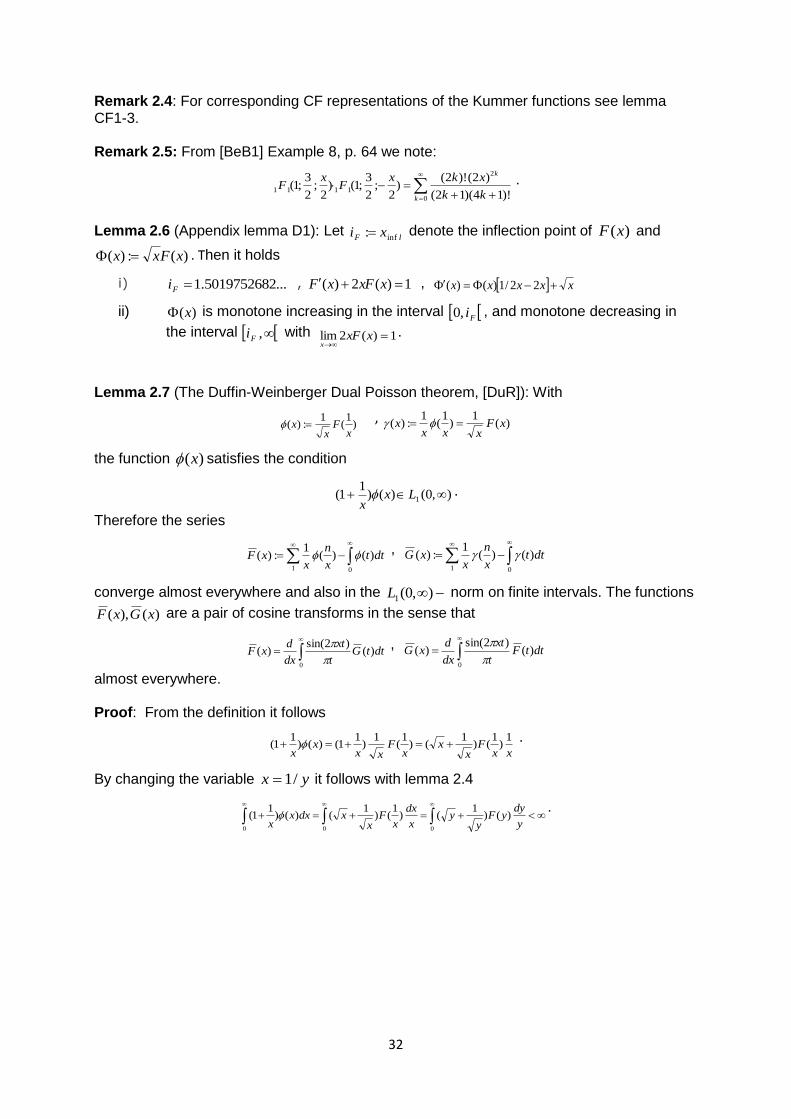
Remark 2.4: For corresponding CF representations of the Kummer functions see lemma CF1-3. Remark 2.5: From [BeB1] Example 8, p. 64 we note:
0
2
1111)!14)(12(
)2()!2()
2;
2
3;1()
2;
2
3;1(
k
k
kk
xkxF
xF .
Lemma 2.6 (Appendix lemma D1): Let lF xi inf: denote the inflection point of )(xF and
)(:)( xFxx . Then it holds
i) ...5019752682.1Fi , 1)(2)( xxFxF , xxxxx 22/1)()(
ii) )(x is monotone increasing in the interval Fi,0 , and monotone decreasing in
the interval ,Fi with 1)(2lim
xxFx
.
Lemma 2.7 (The Duffin-Weinberger Dual Poisson theorem, [DuR]): With
)1
(1
:)(x
Fx
x , )(
1)
1(
1:)( xF
xxxx
the function )(x satisfies the condition
),0()()1
1( 1 Lxx .
Therefore the series
01
)()(1
:)( dttx
n
xxF ,
01
)()(1
:)( dttx
n
xxG
converge almost everywhere and also in the ),0(1L norm on finite intervals. The functions
)(),( xGxF are a pair of cosine transforms in the sense that
0
)()2sin(
)( dttGt
xt
dx
dxF
,
0
)()2sin(
)( dttFt
xt
dx
dxG
almost everywhere. Proof: From the definition it follows
xxF
xx
xF
xxx
x
1)
1()
1()
1(
1)
11()()
11(
.
By changing the variable yx /1 it follows with lemma 2.4
000
)()1
()1
()1
()()1
1(y
dyyF
yy
x
dx
xF
xxdxx
x
.
33
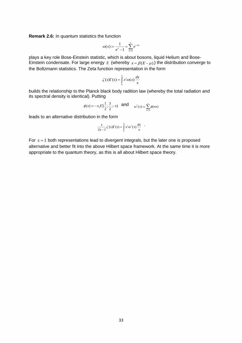
Remark 2.6: In quantum statistics the function
01
1:)(
n
nx
xe
ex
plays a key role Bose-Einstein statistic, which is about bosons, liquid Helium and Bose-Einstein condensate. For large energy E (whereby )( Ex ) the distribution converge to
the Boltzmann statistics. The Zeta function representation in the form
0
)()()(x
dxxxss s
builds the relationship to the Planck black body radition law (whereby the total radiation and its spectral density is identical). Putting
),2
3;
2
1(:)( 11 xFxx and
0
* )(:)(n
nxx
leads to an alternative distribution in the form
0
* )()()(12 x
dxxxss
s
s s .
For 1s both representations lead to divergent integrals, but the later one is proposed
alternative and better fit into the above Hilbert space framework. At the same time it is more
appropriate to the quantum theory, as this is all about Hilbert space theory.
34
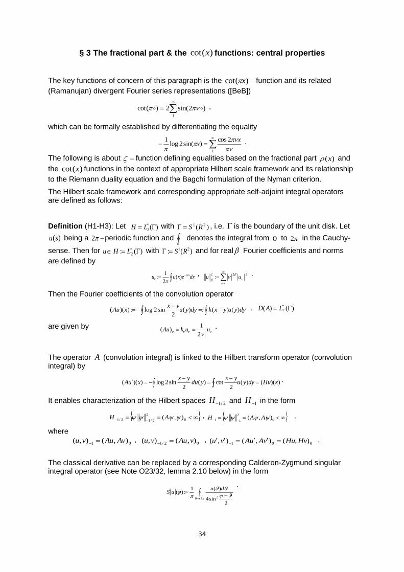
§ 3 The fractional part & the )cot(x functions: central properties
The key functions of concern of this paragraph is the )cot( x function and its related
(Ramanujan) divergent Fourier series representations ([BeB])
1
)2sin(2)cot( ,
which can be formally established by differentiating the equality
1
2cos)sin(2log
1
xx .
The following is about function defining equalities based on the fractional part )(x and
the )cot(x functions in the context of appropriate Hilbert scale framework and its relationship
to the Riemann duality equation and the Bagchi formulation of the Nyman criterion.
The Hilbert scale framework and corresponding appropriate self-adjoint integral operators are defined as follows: Definition (H1-H3): Let )(*
2 LH with )( 21 RS , i.e. is the boundary of the unit disk. Let
)(su being a 2 periodic function and denotes the integral from 0 to 2 in the Cauchy-
sense. Then for )(: 2 LHu with )(: 21 RS and for real Fourier coefficients and norms
are defined by
dxexuu xi
)(2
1:
,
222
:
uu
.
Then the Fourier coefficients of the convolution operator
dyyuyxkdyyuyx
xAu )()(:)(2
sin2log:))((
, )()( *2 LAD
are given by
uukAu
2
1)( .
The operator A (convolution integral) is linked to the Hilbert transform operator (convolution integral) by
))(()(2
cot)(2
sin2log))(( xHudyyuyx
yudyx
xuA
.
It enables characterization of the Hilbert spaces 2/1H and 1H in the form
0
2
2/12/1 ),( AH , 0
2
11 ),( AAH ,
where
01 ),(),( AvAuvu ,
02/1 ),(),( vAuvu ,
001 ),(),(),( HvHuvAuAvu
.
The classical derivative can be replaced by a corresponding Calderon-Zygmund singular integral operator (see Note O23/32, lemma 2.10 below) in the form
20 2
2sin4
)(1:)(
duuS
.
35
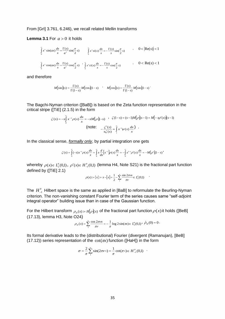
From [GrI] 3.761, 6.246), we recall related Mellin transforms
Lemma 3.1 For 0a it holds
)2
sin()(
)sin(0
sa
s
x
dxaxx
s
s
)
2sin(
)()(
0
ss
s
x
dxxsix s
, 1)Re(0 s
)2
cos()(
)cos(0
sa
s
x
dxaxx
s
s
, )
2cos(
)()(
0
ss
s
x
dxxcix s
, 1)Re(0 s
and therefore
)1(cos)1(
)()(sin sM
s
ssM
, )1(sin)1(
)()(cos sM
s
ssM
.
The Bagchi-Nyman criterion ([BaB]) is based on the Zeta function representation in the critical stripe ([TiE] (2.1.5) in the form
)()()(0
ssMx
dxxxss s
, )1()()1()1()1( sxxMsMss
(note:
1
)()(
)(
x
dxxx
ss
s s
) .
In the classical sense, formally only, by partial integration one gets
0
1
00
)1()()()()()( sMx
dxxx
x
dxxx
dx
dx
x
dxxxss sss
,
whereby )1,0()( #
2Lx , )1,0()( #
1 Hx (lemma H4, Note S21) is the fractional part function
defined by ([TiE] 2.1) )1,0(
2sin
2
1::)( #
2
1
Lx
xxxx
.
The #
1H Hilbert space is the same as applied in [BaB] to reformulate the Beurling-Nyman
criterion. The non-vanishing constant Fourier term of the series causes same “self-adjoint integral operator” building issue than in case of the Gaussian function.
For the Hilbert transform )(:)( xHxH of the fractional part function )(x it holds ([BeB]
(17.13), lemma H3, Note O24) )1,0()sin(2log
12cos)( #
2
1
Lxx
xH
, 0)0(ˆ H .
Its formal derivative leads to the (distributional) Fourier (divergent (Ramanujan), [BeB]
(17.12)) series representation of the )cot( x function ([HaH]) in the form
)1,0()cot(1
)2sin(2 #
1
1
H
.
36
Note: Putting
)1(
1)
2tan()1()
2cos()2(2)1()
2sin()2(2
)2
(
)2
1(
:)( 11
2
2
1
ssssss
s
s
s ss
s
s
)2
cot()(:)(* sss
it holds
)1()()( sss
whereby 1)1()()1()( ** ssss .
Lemma 3.2 For 1)1Re(0 s it holds
s
ss
s
s
s
s
s
s
s
ss
xMsxM
s
s
s
H
)()(
)2
(
)2
1(
2)(
)2
(
)2
1(
)1(
)(2)1()
2cos)1()(
2
1
1
Proof: With lemma 3.1. one gets
)())2
sin(1
()(
)2(
1)1()
2cos)1()(
11
sss
ss
xMsxM
sH
and therefore
s
ss
s
s
s
s
s
s
s
ssxM
s
s
s
H
)()(
)2
(
)2
1(
2)(
)2
(
)2
1(
)1(
)(2)1()(
2
1
.
. Remark 3.1: From [IvA] (A.26) we recall
Let )(xg be a function of real variable x with bounded first derivative on ba, . Then
the Fourier expansion
1
)2sin()(
xxB
fulfills the equality
1
)2cos()(2)()(
b
a
b
a
dxxxgdxxgxB .
From [LaG] we recall the quote from D. Hilbert
„an (unbounded) normal operator D of an Hilbert space H is self-adjoint if and only if its spectrum Spec(D), which is a closed subset of the complex plane, is included in the real line” ( “and with this, Sirs, we shall prove the RH”).
37
Lemma 3.3: The Mellin transform of the (convolution) distribution
)1,0()2sin(2)cot()()( #
1
1
Hxxxx H
defines a corresponding distribution valued Zeta function in a weak )1,0(#
1H sense (in the
critical stripe) given by
)1()()1()()2
cot()1()( * ssssssxM H
resp. )()1()()1()
2tan()()( * ssssssxM H
Proof: With Lemma A8, O23/32, [GrI] 3.761, one gets
)1()2
cos()1()2(2sin1
)2(22sin2)1()( 1
0
1
11
1
0 1
1 sssy
dyyy
x
dxxxsxM ss
s
ss
H
whereby
)1()2
cos()2(2)2
cot()( 1 ssss s
.
Putting
)1()(:)( sxMs HH .
one gets )1()()1()( ssss HH
and therefore Corollary 3.1: )(s and )(sH have the same zeros.
Remark 3.2 ([TiE] 4.14): It holds
)(1
1)(
1
xOs
x
ns
s
sx
uniformly for 00 , Cxt /2 , when C is a given constant greater than 1 . The proof of
this theorem is built on the identity (see also [McC], [BeB] 5)
ix
ix
s
xns z
dzzz
in)cot((
2
11 1
.
The function )cot( x is holomorphic except the pole 1z .
The distributional Hilbert space #
1H plays a key role in [BaB], where the Nyman criterion is
reformulated within a purely functional analysis weighted 2l Hilbert space framework.
Remark 3.3: The considered Hilbert space in [BaB] is about of all sequences Nnaa n of
complex numbers such that
1
2
n
nn a with 2
2
2
1
n
c
n
cn
which is isomorph to the Hilbert space 1
21
lH .
38
Remark 3.4: Let
,......1,1,11:
then it holds
6
1 2
12
2
1
n
i.e. 1
2
l .
With respect to the concept of summability of Fourier series and related double infinite regular matrix in the form
k we refer to [ZyA] III.
Theorem (Bagchi-Nyman criterion, [BaB]): Let
,....3,2,1)(: nk
nk
for ,...3,2,1k
and k be the closed linear span of k . Then the Nyman criterion states that the
following statements are equivalent:
i) The Riemann Hypothesis is true
ii) k .
Remark 3.5: With respect to the concept of summability of Fourier series and related double infinite regular matrix in the form
k we refer to [ZyA] III.
Alternatively to the double infinite matrix
k above, we propose the analog defined double
infinite matrix
,....3,2,1)/(: nknH
H
k for ,...3,2,1k .
As it holds
012/1),( vuvu
,
the inner product 2/1),( vu is defined for any 1
2
lu , 2
0
2 llv .
Putting (see also Claussen integral function, cardinal series)
1
2: lu , 2))sin(2log(: Ldv
leads to a weak
#
2/1H representation of the )2/1(:)( itt function on the critical line in the
form
),(),(),(),(),(),(),( 002/12/12/1 HHHHH
H
k SSd .
As 2/1
2
l is dense in 1
2
l with respect to the 1
2l norm, belongs to the closed linear span of
Nk
H
k , i.e.
1
2/1
2
1
2
ll
which fulfills the Bagchi criterion. For a corresponding Ritz-Galerkin approximation method (which contains spectral, collocation and linear interpolation approximation methods) with corresponding “optimal” approximation behavior we refer to [BrK].
39
Remark 3.6: Assuming that (*)
1
1
n
nn aan
then there are continuous functions )(),( tt such that (appendix, ([WhJ])
1
0
0 )(tda ,
1
0
)()cos(2 tdntaa nn ,
1
0
)()sin(2 tdntaa nn
i.e.
1
0
)()sin()()cos( tdnttdntan .
A cardinal series in the form
1
0 )1(2
)sin(
n
nnn
nz
a
nz
aaz
represents an entire function (appendix). Given a function )(xf in the form
1
0
)()sin()()cos()( tdxttdxtxf
the series
1
)()()1(
)0()sin(
n
n
nx
nf
nx
nf
x
fx
is (C,1)-summable and its sum is )(xf . If (*) is satisfied, the cardinal series
1
0 )1()sin(
n
nnn
nx
a
nx
a
x
ax
is absolutely convergent. As a prominent example we mention the series representation
)11
(1
)cot(1 nxnxx
xn
.
We consider the Fourier-Stieltjes coefficients for the Claussen integral function (Notes O28, O35), i.e. we put
1
)2cos())sin(2log(
1)(:)(
k
Hk
kxdxxxxd
0:)( xd .
It holds ([GrI] 4.384)
0
0
2
10
)2cos()sin(2log
1
0
n
n
n
dxxnx
0))12cos(()sin(log)2sin()sin(log
1
0
1
0
dxxnxdxxnx
resp. 00 a ,
naa nn
2
1
.
The corresponding (absolute convergent) cardinal series (see also lemma A10) is given by
1 2)(1
12)1(
)sin(1
n
n
x
nnx
x
x
.
The related orthogonal (“discontinuous integrals”) equations for the xsin2log and the
)(log x functions are given by ([NiN] Bd. 1, §87, 89, Bd. 2, §21)
ndxxsixn
2
1)()cos(
0
.
The modified Lommel polynomials provide a corresponding orthogonality polynomials system ([DiD], [ChT] 7, II).
40
Remark 3.7: Assuming that
2
log
n
nn aan
n
there is an analog cardinal series representation (appendix, ([WhJ]). We note the relationship to the Ramanujan formula ([EdH] 10.10, lemma A10), e.g.
0 1
))(1(log)sin(
)( dxxnxxs
ss
n
ns
.
For the relationship to the Mellin inverse theory we refer to [NiN] Bd. 2, §21.
From the theory of Fourier series we recall that for a bounded variation function )(xg with
domain ba, it holds (see also Notes S33, S36-38, S47)
k
b
abna
dykyygngng
)2cos()(2
)0()0(,
. For the Claussen integral ([AbM] 27.8)
1
2
0
)2sin()sin(2log(2:)2(
n
x
n
nxdxxxw
, 10 x
it holds a related (additive) equality to ([BrT])
)2
cot(2
1)
2cot(
2
1cot
xxx
in the form
))1(()()2(2
1xwxwxw .
Remark 3.8: We note that with respect to the )1,0(#
2L inner product the adjoint (in a
distributional
#
2/1H sense) Fourier series representation of the (distributional) Fourier series
representation of
)cot(1
)2sin(2
1
is given by
)(sin
1)2sin(4
21
*
.
Remark 3.9: Let
0)(sin4
1:)(
2
xxg
.
then it holds
))(log(2
1))(sin4log(
2
1)sin(2log( 2 xgxx .
41
The relationship to the concept of quasi-asymtotics of distributions ([VlV] p. 56/57 [PoG3], [SeA1] is given in
Lemma 3.4: It holds
1)cot()(
)(
2
1
xxx
xg
xgx
.
Therefore )(xg is auto-model (or regular varying) of order 1 , i.e.
axg
axg
x
1
)(
)(lim
.
With respect to the Tauberian theorems this results into the asymptotic
2loglog1
2log))sin(2log()sin(2(glo)cot(2/12/12/1
xdtt
xdttdtt
xxx
i.e. xx log))sin(2log(
which is equivalent to ([EdH] 12.7, Tauberian theorems)
2/1
1
2/1
1 ))sin(2log( dxxxdx .
42
§ 5 #
2/1H & Hardy space isometry and Dirchlet series
Dirichlet series of type n are of the form
1
)(s
nneasd
where Nnn
is a sequence of real increasing numbers whose limit is infinity, and its
is a complex variable whose real and imaginary part are and t .
Local properties of certain Hilbert spaces of Dirichlet series and the properties of the )cot( x
function resp. the related )(xG function (lemma S3) to Dirichlet series are given in [OlJ] and
[BaB1], 4.8 lemma.
The relationship between the Dirichlet series theory ([HaG)] and the distributional Hilbert
space
#
2/1H norm is given by [LaE] §227, Satz 40):
Theorem 40: The Dirichlet series
1
log:)( ns
neasf
1
log:)( ns
nebsg
are convergent for s ( 0 ). Then on the critical line it holds
1
2/1
1)2/1()2/1(
2
1lim:, nnba
ndtitgitfgf
whereby for nybnyayh nnn 2sin2cos:)( it holds
dyyx
yh
nxh n
n
1
0
2 ))((sin4
)(2)(
.
. Putting
)2
1(:)( itt
we recall from [EdH] 9.2, 9.8:
t
it
log
)( is bounded for 2,1 t ,
)()( 4/1tOt and
log)(2
1 2dtt .
In the context of the above Dirichlet series this then leads to the identities
T
T nT n
dttT 1
2
2/1
2)1(
1)(
2
1lim
and
6)2(
1 2
12
2
1
n n
,
enabling corresponding convolution representation of corresponding singular integral
operator ([CaD]).
43
The dual space of 2
2/1
22/1
*
2/1 LlHH is isometric to the classical Hardy space H2 (see
also note S48) of analytical functions in the unit disc with norm
drere i
H
i2
** )(2
1:)(
2
.
It holds
i) If * H2 then there exists boundary values ),()(lim)( 2
*
1
*
Lree i
r
i with
22
)(**
L
i
He
ii) If 2/1
* )( Heue ii
, then its Dirichlet extension into the disc is given by ( irez )
)()(:)(11
zuzueruzU i
with 2
2/1
*22
0
uU .
The dual spaces 2
* LH ( 2/1 , 1 ) are proposed as appropriate framework for
Schnirelmann densities to apply probability methods to analyzing additive number theory problems ([KaM]). Remark 4.1: From [ZyA] XVIII, 11 we recall (see also Notes 37/38):
- If then the set of points of diverngence of the trigonometric series is of outer logarithmic capacity 0 .
- Let O be an open set, and d a mass distribution concentrated in O . If
i)
2
0
)()))(2
1sin(2log(
2
1Mydyx
for all x ,
ii)
1
22
n
nn ban ,
iii) )(xn is any Borel measurable function taking only non-negative
integral values,
then the partial sums )(xsn of
1
)sin()cos(n
nn nxbnxa
satisfy AMydxs xn )()(
12
0
)(
where A is an absolute constant. Remark 4.2: In harmonic analysis by
dwds
w
wdxdyzdhba
B B
)()()(
4
1)(
2
1)(
2:
2
2
22
1
22
the energy of the harmonic continuation )(h to the boundary is given.
1
22
n
nn baa
44
Remark 4.3: There is a generalizing Hilbert scale definition to the norms (definition H1),
which can be applied to the generalized Dirichlet series theory for corresponding distributional representations. It is defined by the inner product resp. norm ( 0t )
),)(,(:),( )( ii
t
t yxeyx i
resp.
)(
2
)(),(: tt
xxx .
Obviously it holds
xtcxt
),()(
. On the other side any negative norm, i.e.
x with
0 , is bounded by the 0 norm and the new )(t norm, i.e. it holds
Lemma 4.1: i) Let 0 be fixed. The )( norm of any
0Hx is bounded by
2
)(
/2
0
22
t
t xexx
with 0 being arbitrary. Let 0, t be fixed. To any 0Hx there is an
1Hy
according to
xyx , xy 1
1
, xeyx t
t
/
)(
.
and therefore
xexxexE t
t
t
St
2/
)(0
2/ 4inf:)(
.
From the above it follows with 2/1;0 t
Corollary 4.1: i) To any 0Hx there is an
1Hy according to
i) xyxyxt
)(0, , xty 1
1
ii) 2
)(
2
0
2
2/1 txextx
Remark 4.4: Polynomials orthogonal on the unit circle ([SzG] 11) are given in Note S49.
Remark 4.5: Let n be the ordinates of s with 0)Im( s and let 0A be according to
)(log#:)( TOTTATTN nn
then ([LaE] VII, 11, §4/5, Notes S44/45):
- the series
1
)sin(:)(
n
z
n
n nez
zS
is absolute convergent for 0z with
0sin
1log
)(lim
00
due
u
uA
z
zS u
z
- the function
1
1:)(
n
z
n
nezf
is regular for 0z .
45
Appendix
Lemma A1 ([GrI] 3.952, 4.352, 4.424):
i)
)
4;
2
3;
21()
2
1(
2
)sin(2
11
0 2
1
41
2
2
Fe
dxxex x , 0)Re( , 1)Re(
ii) )
4;
2
1;
2(
2
)2
(
)cos(2
11
0 2
1 2
Fdxxex x , 0 , 0)Re( , 0)Re(
iii)
ln)()(1
ln0
1
xdxex x , 0)Re( , 0)Re( [GrI] 4.352
iv)
2)()()(
2sin
)()sin()(ln 2
0
12
ctga
dxxaxx [GrI] 4.424
22)(ln
2lnln)(2
aactga , 0a , 1)Re(0
and therefore especially
0
2/12
0
)2sin()(ln2
dxdxxxe
dctgctge 22
0
2/1 )2ln(24
)2ln()2ln()2
1(2
4)
2
1(
2
1)
2
1()
2
1(
4sin
2
2
Lemma A2 ([GrI] 7.612):
)(
)()(
)(
)(),,(
0
11
1
bc
bab
a
cdttcaFtb
, )Re()Re(0 ab .
Lemma A3 ([LeN] 9):
n
nkkk
k
aia zOzk
caaze
ac
czcaF
0
1
11 )(!
)1()()1(
)(
)(),,(
n
nkkk
k
acac zOzk
acaze
a
c
0
1)()( )(!
)()1()1(
)(
)( .
Lemma A4 ([SeA]): For the zeros of degenerate hypergeometric functions ),;(11 zcaF it holds
1. Suppose that 11 aca and 2c if 1a . Then all zeros of ),;(11 zcaF lie in the
half-plane 2)(11)Re( acaz
2. Suppose that 10 a , ac 1 , moreover 2c if 1a . Then all zeros of ),;(11 zcaF
lie in the half-plane 211)Re( aacz
3. Suppose that 10 a , aca 1 , moreover 2c if 1a . Then all zeros of
),;(11 zcaF lie in the horizontal strips nzn 2)Im()12( .
46
Lemma A5 ([LeN] 3, 9.13):
i) xexaaF ),,(11
ii) ),2
3,
2
1()( 2
11 xFxxerf , ),2
3,1()( 2
11 xFxxF
iii) x
xxEixFxxli
log)(log)log,1,1()( 11 resp.
x
exEi
x
)( for x
iv) x
ec
xcxF
x
2111
1),
2
3;
2
1( resp. for x , lemma A3
v) ),2
3;
2
1(),
2
3;1( 1111 xFxxF for x .
Lemma A6 ([EdH] 1.14): For the )(1 xli function and the remaining term of the famous
Riemann function it holds
dsxs
s
ds
d
xit
dt
t
dtixliixlixli s
ia
ia
x
)1log(
log
1
2
1
logloglim)0(0(
2
1)(
1
1
1
00
1
dsxs
s
ds
d
xittt
dt s
ia
iax
)2
1(log
log
1
2
1
log)1( 2
.
Lemma A7 ([[BuH] p. 184): Let n denote the infinite set of zeros of ),;(11 zbaF . Then it
holds
1
11
)(
1)1(
)(
),;(
be
ze
b
zbaFn
z
n
zb
a
.
Lemma A8 ([GrI] 3.761, 6.246): For 0a it holds
)2
sin()(
)sin(0
sa
s
x
dxaxx
s
s
)2
sin()(
)(0
ss
s
x
dxxsix s
, 1)Re(0 s
)2
cos()(
)cos(0
sa
s
x
dxaxx
s
s
,
)2
cos()(
)(0
ss
s
x
dxxcix s
, 1)Re(0 s
and therefore
)1(cos)1(
)()(sin sM
s
ssM
)1(sin
)1(
)()(cos sM
s
ssM
.
47
Lemma A9 ([EdH] 1.3):
1
1 )1
1()1()1( s
nn
ss ,
1
)(
)1()1(
1n
ss
en
s
s
and therefore e.g.
1
1
2
21 )
11()
4
)1(1()1(
)1(
)2
1()
2
1(
s
nn
s
n
s
s
ss
.
Lemma A10 (Ramanujan’s Master Theorem ([BeB] IV, Entry 11): If 0n , then
)()()(!
)(
0 0
nnx
dxx
k
kx kn
)sin(
)()()(
0 0 n
n
x
dxxkx kn
.
Lemma A11 ([EdH] 1.8): If in the critical stripe there is a representation of convergent (Mellin transform) integrals in the form
0
1
0
)()()(x
dxxx
x
dxxxsg ss
,
then there is a power series representation of )(sg
0
2
2 )2
1()
2
1(
n
n
n saitg
with
x
dx
n
xxxa
n
n
0
22/1
2)!2(
)(log)(: .
Proof ([EdH] 1.8):
0
2/12/12/1
0
1 )(2
1)(
2
1)(
x
dxxxxx
x
dxxxxsg ssss
0
2/1
0
log)2/1(log)2/1(2/1 )(log)2
1(cosh)(
2
1
x
dxxxsx
x
dxxeex xsxs
0 0
2
2/1 )()!2(
log)2
1(
x
dxx
n
xs
x
n
.
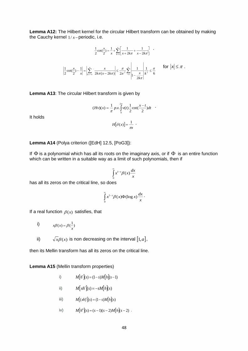
48
Lemma A12: The Hilbert kernel for the circular Hilbert transform can be obtained by making the Cauchy kernel x/1 periodic, i.e.
1 2
1
2
11)
2cot(
2
1
k kxkxx
x
.
6
1
21
1
2)2(2
1)
2cot(
2
122
'
k
k
xkxk
x
x
x
k
for x .
Lemma A13: The circular Hilbert transform is given by
2
0
)2
cot(2
1)(..
1))(( dt
txtvvpxHv .
It holds
x
xH
1
)( .
Lemma A14 (Polya criterion ([EdH] 12.5, [PoG3]):
If is a polynomial which has all its roots on the imaginary axis, or if is an entire function which can be written in a suitable way as a limit of such polynomials, then if
0
1 )(x
dxxx s
has all its zeros on the critical line, so does
0
1 )(log)(x
dxxxx s .
If a real function )(x satisfies, that
i) )1
()(x
xx
ii) )(xx is non decreasing on the interval a,1 ,
then its Mellin transform has all its zeros on the critical line. Lemma A15 (Mellin transform properties)
i) )1()1()( shMsshM
ii) )()( shsMshxM
iii) )()1()()( shMssxhM
iv) )2()2)(1()( shMssshM .
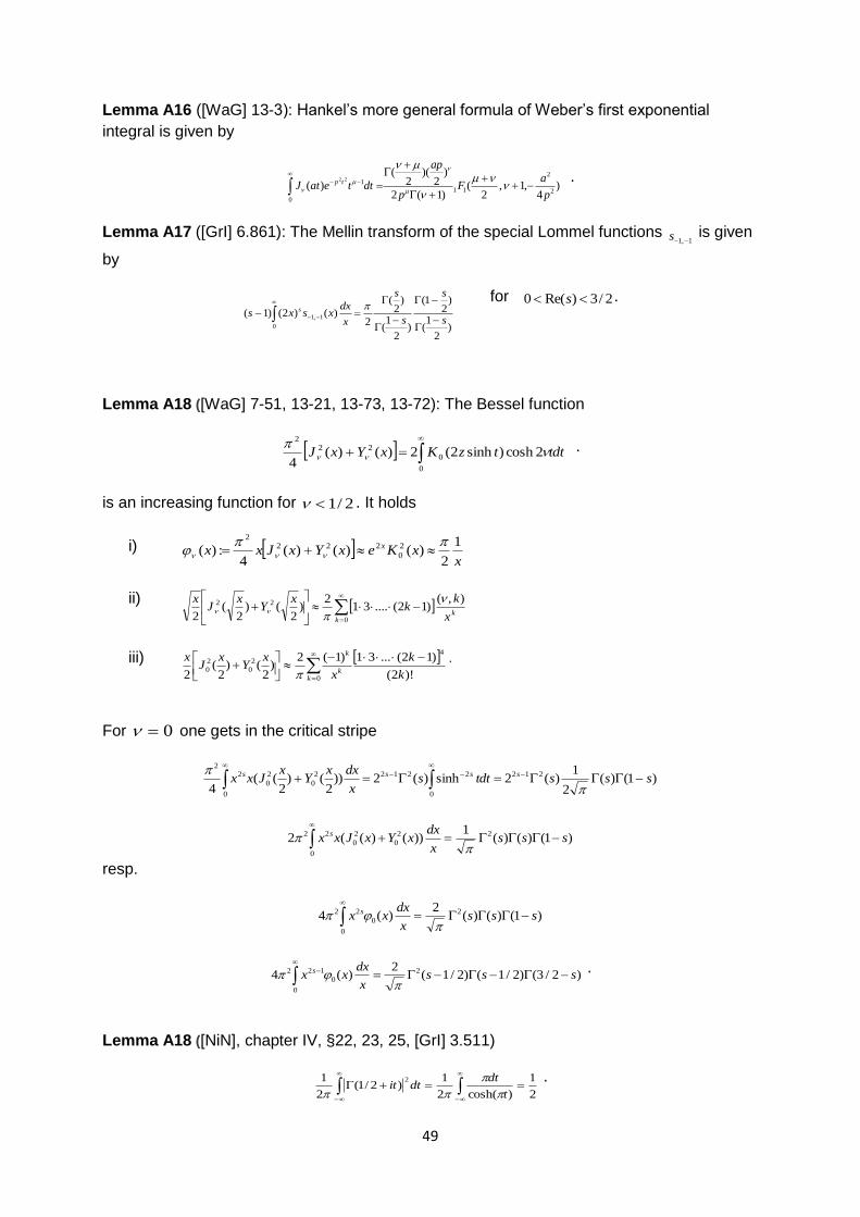
49
Lemma A16 ([WaG] 13-3): Hankel’s more general formula of Weber’s first exponential
integral is given by
0
2
2
11
1 )4
,1,2
()1(2
)2
)(2
(
)(22
p
aF
p
ap
dtteatJ tp
.
Lemma A17 ([GrI] 6.861): The Mellin transform of the special Lommel functions 1,1 s is given
by
)2
1(
)2
1(
)2
1(
)2
(
2)()2()1(
0
1,1 s
s
s
s
x
dxxsxs s
for 2/3)Re(0 s .
Lemma A18 ([WaG] 7-51, 13-21, 13-73, 13-72): The Bessel function
0
0
222
2cosh)sinh2(2)()(4
tdttzKxYxJ
.
is an increasing function for 2/1 . It holds
i) x
xKexYxJxx x 1
2)()()(
4:)( 2
0
2222
ii)
0
22 ),()12(....31
2)
2()
2(
2 kkx
kk
xY
xJ
x
iii)
0
4
2
0
2
0)!2(
)12(...31)1(2)
2()
2(
2 kk
k
k
k
x
xY
xJ
x
.
For 0 one gets in the critical stripe
)1()(2
1)(2sinh)(2))
2()
2((
4
212
0
22122
0
0
2
0
22
ssstdtsx
dxxY
xJxx ssss
)1()()(1
))()((2 22
0
0
2
0
22 sssx
dxxYxJxx s
resp.
)1()()(2
)(4 2
0
0
22 sssx
dxxx s
)2/3()2/1()2/1(2
)(4 2
0
0
122 sssx
dxxx s
.
Lemma A18 ([NiN], chapter IV, §22, 23, 25, [GrI] 3.511)
2
1
)cosh(2
1)2/1(
2
1 2
t
dtdtit
.
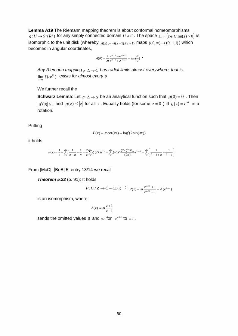
50
Lemma A19 The Riemann mapping theorem is about conformal homeomorphisms
)(: 21 RSUg for any simply connected domain CU . The space 0)Im(: zCz is
isomorphic to the unit disk (whereby )1/()1(:)( zzizA maps )1,1,0(),0,( i ) which
becomes in angular coordinates,
)2
tan(2
2)(
2/2/
2/2/
ii
ii
ee
ee
iA
.
Any Riemann mapping Cg : has radial limits almost everywhere; that is,
)(lim1
i
rref
exists for almost every .
We further recall the
Schwarz Lemma: Let :g be an analytical function such that 0)0( g . Then
1)0( g and zzg )( for all z . Equality holds (for some 0z ) iff iezg )( is a
rotation. Putting
))sin(2(glo)cot()( xzzP
it holds
1
12
0
2
2
0
2' 1
1
1
)!2(
)2()1()2(
2111)(
zkzkz
n
Bzk
znnzzzP nn
nnk
From [McC], [BeB] 5, entry 13/14 we recall
Theorem 5.22 (p. 91): It holds
)(ˆ/: iCZCP : )(1
1)( 2
2
2iz
iz
iz
eAe
eizP
is an isomorphism, where
1
1:)(
z
zizA
sends the omitted values 0 and for ize 2 to i .
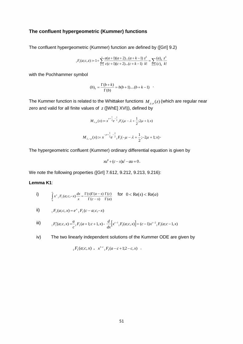
51
The confluent hypergeometric (Kummer) functions
The confluent hypergeometric (Kummer) function are defined by ([GrI] 9.2)
!)(
)(
!)1)...(2)(1(
)1)...(2)(1(1:),;(
01
11k
z
c
a
k
z
kcccc
kaaaazcaF
k
k k
k
k
k
with the Pochhammer symbol
)1)....(1()(
)()(
kbbb
b
kbb k
.
The Kummer function is related to the Whittaker functions )(, zM
(which are regular near
zero and valid for all finite values of z ([WhE] XVI)), defined by
);12;2
1(:)( 11
22
1
, xFexxM
x
);12;2
1(:)( 11
22
1
, xFexxM
x
.
The hypergeometric confluent (Kummer) ordinary differential equation is given by
0)( auuxcux .
We note the following properties ([GrI] 7.612, 9.212, 9.213, 9.216): Lemma K1:
i) )(
)(
)(
)()(),;(
0
11a
c
sc
sas
x
dxxcaFx s
for )Re()Re(0 as
ii) ),;(),;( 1111 xcacFexcaF x
iii) ),1;1(),;( 1111 xcaFc
axcaF , ),1;()1(),;( 11
2
11
1 xcaFxcxcaFxdx
d cc
iv) The two linearly independent solutions of the Kummer ODE are given by
),;(11 xcaF , ),2;1(11
1 xccaFx c .
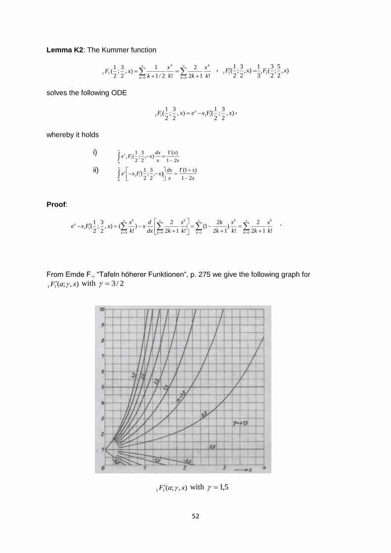
52
Lemma K2: The Kummer function
00
11!12
2
!2/1
1),
2
3;
2
1(
k
k
k
k
k
x
kk
x
kxF , ),
2
5;
2
3(
3
1),
2
3;
2
1( 1111 xFxF
solves the following ODE
),2
3;
2
1(),
2
3;
2
1( 1111 xFxexF x ,
whereby it holds
i)
s
s
x
dxxFxs
21
)(),
2
3;
2
1(
0
11
ii) s
s
x
dxxFxxs
21
)1(),
2
3;
2
1(
0
11
Proof:
0100
11!12
2
!)
12
21(
!12
2)
!(),
2
3;
2
1(
k
k
k
k
k
k
k
kx
k
x
kk
x
k
k
k
x
kdx
dx
k
xxFxe .
From Emde F., “Tafeln höherer Funktionen“, p. 275 we give the following graph for
),;(11 xaF with 2/3
),;(11 xaF with 5,1
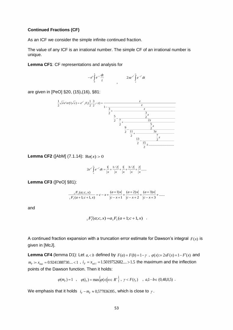
53
Continued Fractions (CF) As an ICF we consider the simple infinite continued fraction. The value of any ICF is an irrational number. The simple CF of an irrational number is unique. Lemma CF1: CF representations and analysis for
x
tx
t
dtee
0 ,
x
tx dtexe22
2
are given in [PeO] §20, (15),(16), §81:
................................2
152
7
2
13
3
2
112
5
2
9
2
2
72
3
2
52
31
),2
3,
2
1()(
2
111
2
z
z
z
z
z
z
z
zzFezerfe zz
Lemma CF2 ([AbM] (7.1.14): 0)Re( x
......22/312/11
222
xxxxxdtee
x
tx
Lemma CF3 ([PeO] §81):
......3
)3(
2
)2(
1
)1(
),1;1(
),;(
11
11
xc
xa
xc
xa
xc
xaxc
xcaF
xcaF
and
),1;1(),;( 1111 xcaFaxcaF .
A continued fraction expansion with a truncation error estimate for Dawson’s integral )(xF is
given in [McJ].
Lemma CF4 (lemma D1): Let ba , defined by 1)()( bFaF , )(1)(2:)( xFxxFx and
1....9241388730.0: max xmF , 5.1....5019752682.1inf lF xi the maximum and the inflection
points of the Dawson function. Then it holds:
1)( Fm , RxxiF )(max)( , )( FrF , )5,0,48,0(1, ba .
We emphasis that it holds 577836395,0 FF mi , which is close to .
54
Hilbert spaces and Hilbert Transformation properties
Let the linear equation ([BrK]) fAu be given in a Hilbert space H with inner product ),(
and norm . The operator is assumed to have the properties
i) A is positive, i.e. 0),( uAu for 0u
ii) A is symmetric, i.e. ),(),( AvuvAu
for )(, ADvu . Then
),(:),( vAuvua
defines an inner product in )(AD with a corresponding norm
),(:2
uuau .
The domain of definition of ),( vua can be extended to AA xHH with
)(: ADH A.
In spectral theory in combination with discrete spectrum deals with the following assumption to the operator A : Let RH
be a Hilbert scale.
1. There is an R such that
a. The mapping HHA 2: is an isomorphism for R , i.e.
22
1
ucAuuc
with some constant c .
b. A is symmetric positive in 0HH , i.e.
2
),(
ucuAu with 0c
2. A is self-adjoint in 0HH , i.e.
),(),( AvuvAu for )(, ADvu .
Note: the differential operator dxd / is not bounded with respect to the norm of )1,0(2L :
for inx
n exf 2:)( it holds 1nf , but nfdxd n 2)(/ .
Definition H1:
Let )(*
2 LH with )( 21 RS , i.e. is the boundary of the unit disk. Let )(su being a 2
periodic function and denotes the integral from 0 to 2 in the Cauchy-sense. Then for
)(: 2 LHu with )(: 21 RS and for real Fourier coefficients and norms are defined by
dxexuu xi
)(2
1: ,
222
:
uu
.
55
Then the Fourier coefficients of the convolution operator
dyyuyxkdyyuyx
xAu )()(:)(2
sin2log:))((
are given by
uukAu2
1)( .
The operator A enables characterization of the Hilbert spaces 2/1H and 1H in the form
0
2
2/12/1 ),( AH , 0
2
11 ),( AAH .
This requires “differentiating / momentum building” of “less regular” “functions than )(: 20 LH
. Hilbert space #
1H can be characterized by the singular integral operator
dyyuyx
xAu )(2
sin2log:))((
, )()( *2 LAD ,
It holds
01 ),(),( AvAuvu ,
02/1 ),(),( vAuvu ,
001 ),(),(),( HvHuvAuAvu
,
whereby
))(()(2
cot)(2
sin2log))(( xHudyyuyx
yudyx
xuA
.
Lemma H1: It holds
i) if n is an orthogonal system of )1,0(#
2L , then nn H : is also an
orthogonal system of )1,0(#
2L
ii) 0,0nn
iii) nn n is an orthogonal system of )1,0(#
1H
iv) for #
0Hg it holds
0001gHggAg
.
Some key properties of the Hilbert transform
dyyx
yuyd
yx
yuxHu
yx
)(1)(1lim:))((
0
are given in (PeB] examples 2.99, 2.9.11)
56
Lemma H2: i) The constant Fourier term vanishes, i.e. 0)( 0 Hu
ii)
dyyuxuxHxxuH )(1
))(())((
iii)
For odd functions it hold
))(())(( xHuxxxuH
v) If
2, LHuu then u and
Hu are orthogonal, i.e.
0))()((
dyyHuyu
v) 1H , HH * ,
IH 2 , 31 HH
vi) gHfHgfgfH **)*( HgHfgf **
vii) If Nnn
is an orthogonal system, so it is for the system NnnH )( ,
i.e. nnnnnn HHH ,,, 2
viii) 22uHu , i.e. if
2Lu , then 2LHu .
Proof: i), v)-viii) see [PeB], 2.9
ii) Consider the Hilbert transform of )(xxu
dyyx
yyuxxuH
)(1))((
.
The insertion of a new variable yxz yields
dyyuxuxHdzzxudzz
zxxudz
z
zxuzxxxuH )(
1))(()(
1)((1)()(1))((
iii) It follows from i) and ii)
iv)
dusigni
dyyHuyu2
)(ˆ)((2
))()(( whereby 2
)(ˆ u is even .
Lemma H3:
i) ttH sin)cos(
ii) ttH cos)sin(
iii) 0)(tan xtconsH
iv) )()()sin(log xxxtH ([MaJ])
Note (www.quantum-gravitation.de) An inner product for differential forms can be defined by
000 ),(),())(),((:)),(( vuHvHudvAduAdvdu .
Corresponding properties of the Hilbert resp. the Riesz operators lead to “rotation invariance of this inner product”. In [GoK] a related cosmological solution of Einstein’s field equations of gravitation is proposed (alternatively to the Schwarzschild metric), which exhibits a rotation of matter relative to the compass of inertia. This is equivalent to the non-existence of the standard cosmological solution with non-vanishing density of matter, which is a system of three-spaces, containing an “absolute” time coordinate. The solution in [GoK] has a sign of the cosmological constant, which is the opposite of that occurring in Einstein’s static solution. It corresponds to a positive pressure.
57
Lemma H4 For the Hilbert transform of the fractional part function
)sin(2log12cos
)(1
xx
xH
it holds #
2LH , and therefor
#
1
1
)2sin(2)cot()(
HxxxH .
Proof: It holds
12
1
2)
2sin(2(log
3
12
0
2
n ndx
x
which follows from the representation
1 1
2 )cos()cos()
2sin(2(log
n k nk
nxkxx ,
in combination with the orthogonality relations
nk
nkodxnxkx
2
)cos()cos(0
.
Note:
1 1
2 )cos()cos()
2sin(2(log
2
1
n k n
nxkxx
dx
d .
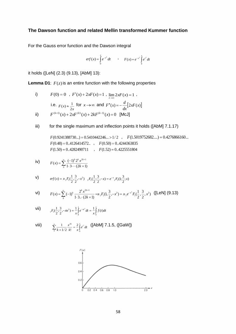
58
The Dawson function and related Mellin transformed Kummer function For the Gauss error function and the Dawson integral
x
t dtexerf0
2
)( ,
x
tx dteexF0
22
)(
it holds ([LeN] (2.3) (9.13), [AbM] 13): Lemma D1: )(zF is an entire function with the following properties
i) 0)0( F , 1)(2)( xxFxF , 1)(2lim
xxF
z
,
i.e. x
xF2
1)( for x and )(2)( xxF
dx
dxF
ii) 0)(2)(2)( )1()()1( xkFxxFxF kkk [McJ]
iii) for the single maximum and inflection points it holds ([AbM] 7.1.17)
2/1...5410442246.0...)9241388730.0( F , ...4276866160.0....)5019752682.1( F
..4126414572..0)48.0( F , 4244363835..0)50.0( F
4282490711..0)50.1( F , 4225551804..0)52.1( F
iv)
0
12
)12(31
2)1()(
k
xxF
kkk
v) ),2
3,
2
1()( 2
11 xFxxerf );2
3;1(),
2
3;
2
1( 1111 xFexF x
vi) ),2
3,
2
1(),
2
3,1(
)12(..31
2)1()( 2
11
2
11
0
122
xFexxFxk
xxF x
kkk
([LeN] (9.13)
vii)
xx
t dttfx
dtex
xF00
2
11 )(11
),2
3;
2
1(
2
viii)
x
tk
dtexk
x
k00
222
!2/1
1 ([AbM] 7.1.5, ([GaW])
59
The relationship between the Kummer the Dawson and the Gaussian functions is given by
Lemma D2: For Rx it holds
0
2
111
2
11 )2sin(),2
3,
2
1(),
2
3,1()(
22
dtxtexFexxFxxF tx .
Putting 2
:)( xexg it holds ([GaW] 7.1.17)
Lemma D3:
i) )(2)( xFxgH
ii) x
xFc
x
eH
x )(
.
Putting
)2
,1,2
12()
2,1,
2
1(:)(
2
11
22
11
2 2 xFx
xFexx x
from ([GrI] (7.641), (7.643)) one gets Lemma D4: For 2/1)Re(,0 y
i) ),2
3,1(
2
1:)( 222
yyedteyerfc y
x
t
, ([LeN] (9.13.1)
ii) )(2
),2
3,1(
4)2cos(),
2
3,1( 2
0
2
11
2
yerfcyyedxxyxF y
iii) )(2
)sin()(0
xdxxyx
.
.
Lemma D5: ([LeN] (9.8.5): ),2,1(1
11 xFx
ex
.
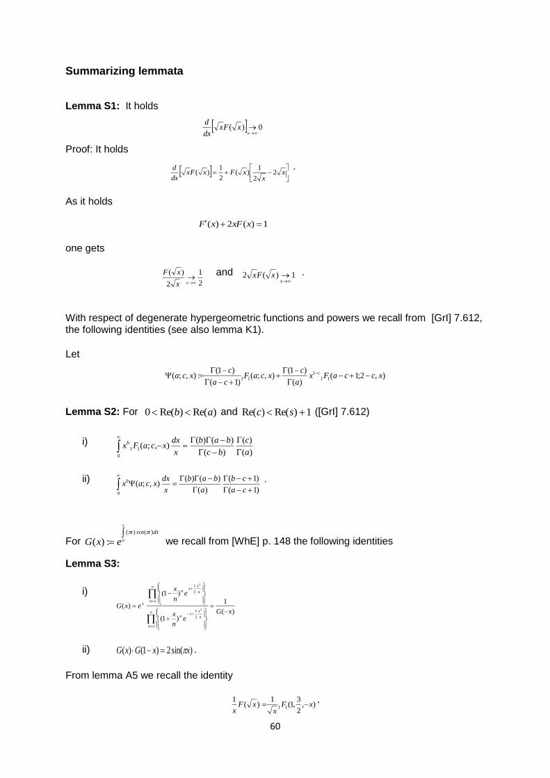
60
Summarizing lemmata
Lemma S1: It holds
0)(
x
xFxdx
d
Proof: It holds
x
xxFxFx
dx
d2
2
1)(
2
1)(
.
As it holds
1)(2)( xxFxF
one gets
2
1
2
)(
xx
xF and 1)(2
x
xFx .
With respect of degenerate hypergeometric functions and powers we recall from [GrI] 7.612, the following identities (see also lemma K1).
Let
),2;1()(
)1(),;(
)1(
)1(:),;( 11
1
11 xccaFxa
cxcaF
ca
cxca c
Lemma S2: For )Re()Re(0 ab and 1)Re()Re( sc ([GrI] 7.612)
i) )(
)(
)(
)()(),;(
0
11a
c
bc
bab
x
dxxcaFxb
ii) )1(
)1(
)(
)()(),;(
0
ca
cb
a
bab
x
dxxcaxb .
For
x
dttt
exG 0
)cot()(
:)(
we recall from [WhE] p. 148 the following identities
Lemma S3:
i)
)(
1
)1(
)1(
)(
1
2
1
1
2
1
2
2
xGe
n
x
en
x
exG
n
n
xx
n
n
n
xx
n
x
ii) )sin(2)1()( xxGxG .
From lemma A5 we recall the identity
),2
3,1(
1)(
111 xF
xxF
x
.
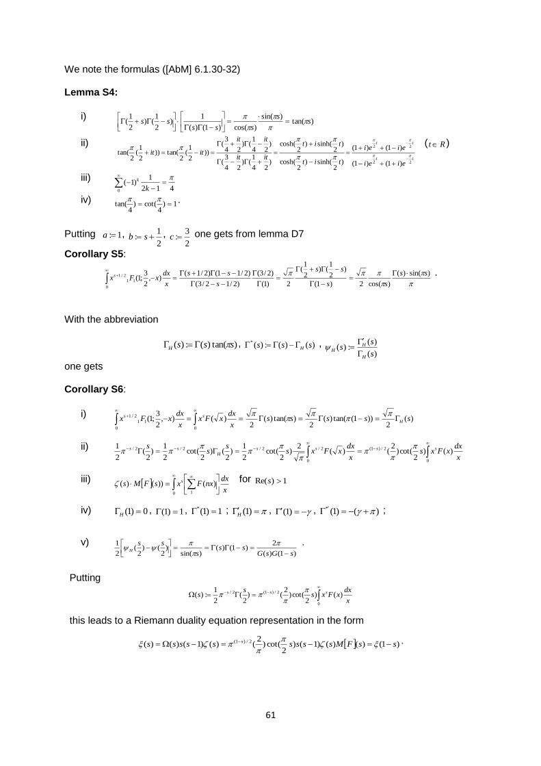
61
We note the formulas ([AbM] 6.1.30-32) Lemma S4:
i) )tan(
)sin(
)cos()1()(
1)
2
1()
2
1( s
s
sssss
ii)
tt
tt
eiei
eiei
tit
tit
itit
itit
itit
22
22
)1()1(
)1()1(
)2
sinh()2
cosh(
)2
sinh()2
cosh(
)24
1()
24
3(
)24
1()
24
3(
))2
1(
2tan())
2
1(
2tan(
( Rt )
iii) 412
1)1(
0
k
k
iv) 1)4
cot()4
tan( .
Putting 1:a , 2
1: sb ,
2
3:c one gets from lemma D7
Corollary S5:
)sin()(
)cos(2)1(
)2
1()
2
1(
2)1(
)2/3(
)2/12/3(
)2/11()2/1(),
2
3;1(
0
11
2/1 ss
ss
ss
s
ss
x
dxxFxs
.
With the abbreviation
)tan()(:)( sssH , )()(:)(* sss H , )(
)(:)(
s
ss
H
HH
one gets Corollary S6:
i) )(
2))1(tan()(
2)tan()(
2)(),
2
3;1(
00
11
2/1 sssssx
dxxFx
x
dxxFx H
ss
ii)
0
2/)1(
0
2/2/2/2/ )()2
cot()2
()(2
)2
cot(2
1)
2()
2cot(
2
1)
2(
2
1
x
dxxFxs
x
dxxFxs
ss
s ssss
H
ss
iii)
0 1
)())()(x
dxnxFxsFMs s
for 1)Re( s
iv) 0)1( H, 1)1( , 1)1(* ; )1(H
, )1( , )()1(* ;
v) )1()(
2)1()(
)sin()
2()
2(
2
1
sGsGss
s
ssH
.
Putting
0
2/)1(2/ )()2
cot()2
()2
(2
1:)(
x
dxxFxs
ss sss
this leads to a Riemann duality equation representation in the form
)1()()()1()2
cot()2
()()1()()( 2/)1( ssFMsssssssss s
.
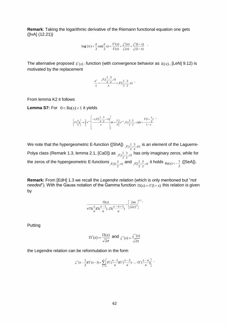
62
Remark: Taking the logarithmic derivative of the Riemann functional equation one gets ([IvA] (12.21))
)1(
)1(
)(
)(
)(
)()
2tan(
2)2log(
s
s
s
s
s
ss
.
The alternative proposed )(* xli function (with convergence behavior as )(xli , [LeN] 9.12) is
motivated by the replacement
),2
3;
2
1(
),2
3;
2
1(
11
11
xFx
xF
x
ex
.
From lemma K2 it follows
Lemma S7: For 1)Re(0 s it yields
s
s
dxxFxdxx
xFx
xs ss
1
)2
1(
),2
5;
2
3(
3
1),
2
3;
2
1(
)2
(0
11
2/
0
112/
.
We note that the hypergeometric E-function ([ShA])
),2
3;
2
1(11 izF
is an element of the Laguerre-
Polya class (Remark 1.3, lemma 2.1, [CaD]) as ),
2
3;
2
1(11 zF
has only imaginary zeros, while for
the zeros of the hypergeometric E-functions),
2
3;1(11 zF
and ),2
3;
2
1(11 zF it holds
2
1)Re( z ([SeA]).
Remark: From [EdH] 1.3 we recall the Legendre relation (which is only mentioned but “not needed”). With the Gauss notation of the Gamma function )1(:)( ss this relation is given
by
2/1
)2(
2
)1
()...1
()(
)(
n
s
n
n
ns
n
s
n
sn
s
.
Putting
2
)(:)(* s
s
and
2
)(:)(
** s
s
the Legendre relation can be reformulation in the form
1
***** )(..)2
()1
()1()2
1(
n n
ns
n
s
n
sss
.
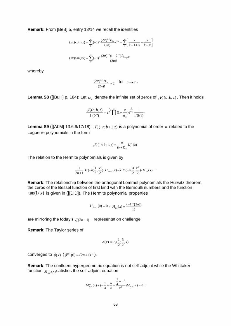
63
Remark: From [BeB] 5, entry 13/14 we recall the identities
1
2
0
2
2
1)!2(
)2()1()cot()(
xk
x
xk
xx
n
Bxx nn
nn
nn
nnn x
n
Bxx 2
0
2
22
)!2(
)21()2()1()tan()(
whereby
2)!2(
)2( 2
2
n
B n
n for n .
Lemma S8 ([[BuH] p. 184): Let
n denote the infinite set of zeros of ),;(11 zbaF . Then it holds
1
11
?)(
1)1(
?)(
),;(
be
ze
b
zbaFn
z
n
zb
a
.
Lemma S9 ([[AbM] 13.6.9/17/18): ),1;(11 zbnF is a polynomial of order n related to the
Laguerre polynomials in the form
)()1(
!),1;( )(
11 xLb
nzbnF b
n
n
.
The relation to the Hermite polynomials is given by
)()2
,2
3;()()
2,
2
1;(
12
12
2
1112
2
11 xHx
nFxxHx
nFn
nn
.
Remark: The relationship between the orthogonal Lommel polynomials the Hurwitz theorem, the zeros of the Bessel function of first kind with the Bernoulli numbers and the function
)/1tan( x is given in ([[DiD]). The Hermite polynomial properties
0)0(12 nH , !
)!2()1()(2
n
nxH
n
n
are mirroring the today’s )12( n representation challenge.
Remark: The Taylor series of
),2
3;
2
1(:)( 11 xFx
converges to )(x ( 1)( )12()0( nn ).
Remark: The confluent hypergeometric equation is not self-adjoint while the Whittaker function )(, xM
satisfies the self-adjoint equation
0)()4
1
4
1()( ,2
2
,
xMxx
xM
.
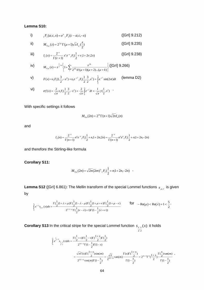
64
Lemma S10:
i) ),;(),;( 1111 xcacFexcaF x ([GrI] 9.212)
ii) )2
()1(2)( 2
,0
zIzzM
([GrI] 9.235)
iii) )2;21,2
1(
)1(
2)( 11 xFexxI x
([GrI] 9.238)
iv)
14
2
2
1
,0))...(2)(1(!2
1)(kk
zzzM
k
k
([GrI] 9.266)
v)
0
2
111
2
11 )2sin(),2
3,
2
1(),
2
3,1()(
22
dtxtexFexxFxxF tx (lemma D2)
vi) ),
2
1(
12),
2
3,
2
1(
2)( 2
0
2
11
2
xdtexFxxerf
x
t
.
With specific settings it follows
)(2)1(2)2( 2
,0 nInnnM n
n
n
and
)2,21;2
1(
)1(
2)2;21,
2
1(
)1(
2)( 1111 nnnFen
nnnnFen
nnI nn
nnn
n
n
and therefore the Stirling-like formula Corollary S11:
)2,21;2
1()2(2)2( 11,0 nnnFennnM n
n .
Lemma S12 ([GrI] 6.861): The Mellin transform of the special Lommel functions
,,s is given
by
))(2
11()1)(
2
1(2
)1(2
1()1(
2
1()1(
2
1()1(
2
1(
)(20
,
1
dxxsx for
2
51)Re()Re( .
Corollary S13 In the critical stripe for the special Lommel function )(2
,2
xs ss it holds
)1()2
1(2
)2
1()
2
1()
2
1()
2
1(
)()1(20 2
,2
12
3
ss
sss
dxxsxs
ss
s
)2
1(
)tan()2
(
)2
1(2
)2
1(
)2
1()(
)tan(2
)2
1()cos(2
)sin()2
1()(
234
)1(2)1(2 s
ss
s
s
ss
ss
s
ss
ss
ss
.
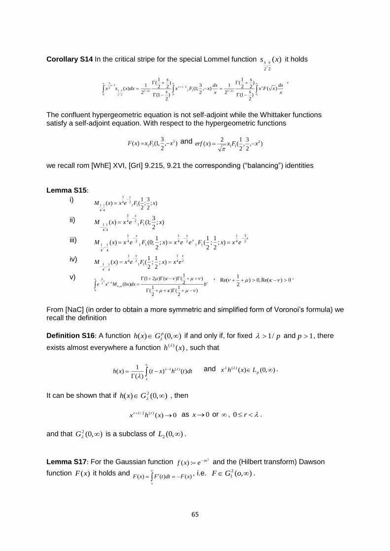
65
Corollary S14 In the critical stripe for the special Lommel function )(2
,2
xs ss it holds
0
21
0
11
2/1
21
0 2,
2
12
3
)(
)2
1(
)22
1(
2
1),
2
3;1(
)2
1(
)22
1(
2
1)(
x
dxxFx
s
s
x
dxxFx
s
s
dxxsx s
s
s
sss
s .
The confluent hypergeometric equation is not self-adjoint while the Whittaker functions satisfy a self-adjoint equation. With respect to the hypergeometric functions
),2
3,1()( 2
11 xFxxF and ),2
3,
2
1(
2)( 2
11 xFxxerf
we recall rom [WhE] XVI, [GrI] 9.215, 9.21 the corresponding (“balancing”) identities
Lemma S15:
i) );
2
3;
2
1()( 11
24
3
4
1,
4
1 xFexxM
x
ii) );2
3;1()( 11
24
3
4
1,
4
1 xFexxM
x
iii) xx
xx
exxFeexxFexxM 2
3
4
1
1124
1
1124
1
4
1,
4
1 );2
1;
2
1();
2
1;0()(
iv) 24
1
1124
1
4
1,
4
1 );2
1;
2
1()(
xx
exxFexxM
v)
bdxbxMxe
xb
)2
1()
2
1(
)2
1()()21(
)(0
,
12
, 0)Re(,0)2
1Re( .
From [NaC] (in order to obtain a more symmetric and simplified form of Voronoi’s formula) we recall the definition
Definition S16: A function ),0()( pGxh if and only if, for fixed p/1 and 1p , there
exists almost everywhere a function )()( xh , such that
x
dtthxtxh )()()(
1)( )(1
and ),0()()( pLxhx .
It can be shown that if ),0()( 2 Gxh , then
0)()(2/1 xhx rr as 0x or , r0 .
and that ),0(2 G is a subclass of ),0(2 L .
Lemma S17: For the Gaussian function 2
:)( xexf and the (Hilbert transform) Dawson
function )(xF it holds and )()()( xFdttFxF
x
, i.e. ),(2
1 oGF .
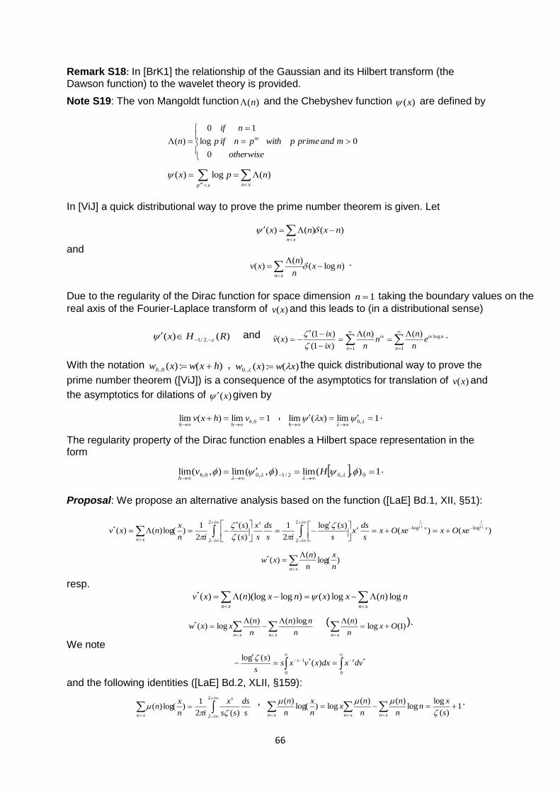
66
Remark S18: In [BrK1] the relationship of the Gaussian and its Hilbert transform (the Dawson function) to the wavelet theory is provided.
Note S19: The von Mangoldt function )(n and the Chebyshev function )(x are defined by
0
1
0
log
0
)(
mandprimepwith
otherwise
pn
n
if
if
pn m
xp xnm
npx )(log)(
In [ViJ] a quick distributional way to prove the prime number theorem is given. Let
)()()( nxnxxn
and
)log()(
)( nxn
nxv
xn
.
Due to the regularity of the Dirac function for space dimension 1n taking the boundary values on the
real axis of the Fourier-Laplace transform of )(xv and this leads to (in a distributional sense)
)()( .2/1 RHx and
1
log
1
)()(
)1(
)1()(ˆ
n
nix
n
ix en
nn
n
n
ix
ixxv
.
With the notation )(:)(0.. hxwxwh , )(:)(..0 xwxw the quick distributional way to prove the
prime number theorem ([ViJ]) is a consequence of the asymptotics for translation of )(xv and
the asymptotics for dilations of )(x given by
1lim)(lim 0,
hhh
vhxv , 1lim)(lim ,0
xh
.
The regularity property of the Dirac function enables a Hilbert space representation in the form
1),(lim),(lim),(lim 0,02/1,00,
Hvhh
.
Proposal: We propose an alternative analysis based on the function ([LaE] Bd.1, XII, §51):
i
i
x
i
i
xss
xn
xeOxxeOxs
dsx
s
s
is
ds
s
x
s
s
in
xnxv
2
2
log
2
2
log* )()()(glo
2
1
)(
)(
2
1)log()()(
11
1
11
1
)log()(
)(*
n
x
n
nxw
xn
resp. nnxxnxnxv
xnxn
log)(log)()log(log)()(*
xnxn n
nn
n
nxxw
log)()(log)(* ( )1(log
)(Ox
n
n
xn
).
We note
0
*
0
*1 )()(glo
dvxdxxvxss
s ss
and the following identities ([LaE] Bd.2, XLII, §159):
i
i
s
xn s
ds
ss
x
in
xn
2
2)(2
1)log()(
, 1
)(
loglog
)()(log)log(
)(
s
xn
n
n
n
nx
n
x
n
n
xnxnxn
.
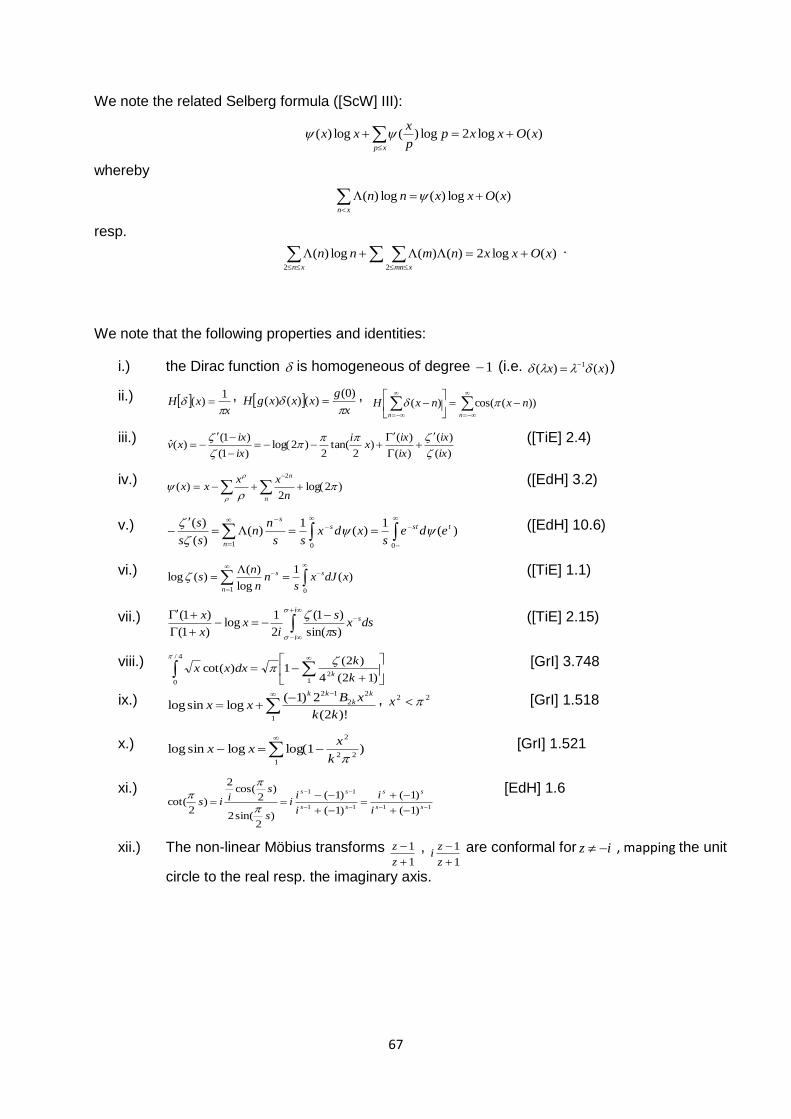
67
We note the related Selberg formula ([ScW] III):
xp
xOxxpp
xxx )(log2log)(log)(
whereby
)(log)(log)( xOxxnnxn
resp.
)(log2)()(log)(22
xOxxnmnnxmnxn
.
We note that the following properties and identities:
i.) the Dirac function is homogeneous of degree 1 (i.e. )()( 1 xx )
ii.) x
xH
1
)( , x
gxxxgH
)0()()()( ,
nn
nxnxH ))(cos()(
iii.) )(
)(
)(
)()
2tan(
2)2log(
)1(
)1()(ˆ
ix
ix
ix
ixx
i
ix
ixxv
([TiE] 2.4)
iv.)
n
n
n
xxxx )2log(
2)(
2 ([EdH] 3.2)
v.)
001
)(1
)(1
)()(
)( tsts
n
s
edes
xdxss
nn
ss
s
([EdH] 10.6)
vi.)
01
)(1
log
)()(log xdJx
sn
n
ns s
n
s ([TiE] 1.1)
vii.)
i
i
sdsxs
s
ix
x
x
)sin(
)1(
2
1log
)1(
)1( ([TiE] 2.15)
viii.)
4/
0 12 )12(4
)2(1)cot(
k
kdxxx
k
[GrI] 3.748
ix.)
1
2
2
12
)!2(
2)1(logsinlog
kk
xBxx
k
k
kk
, 22 x [GrI] 1.518
x.)
1
22
2
)1log(logsinlogk
xxx [GrI] 1.521
xi.) 1111
11
)1(
)1(
)1(
)1(
)2
sin(2
)2
cos(2
)2
cot(
ss
ss
ss
ss
i
i
i
ii
s
siis
[EdH] 1.6
xii.) The non-linear Möbius transforms 1
1
z
z , 1
1
z
zi are conformal for iz , mapping the unit
circle to the real resp. the imaginary axis.
68
Note S20: In [PoG3] the following general theorem about zeros of the Fourier transform of a real function is given:
Theorem 5: Let ba be finite real numbers and let )(tg be a strictly positive
continuous function on the open interval ba, and differentiable in ba, except
possibly at finitely many points. Suppose that
)(
)(
tg
tg
at every point of ba where )(tg is differentiable. Then every zero of the integral
b
a
ztdtetgzg )()(ˆ
lies in the open infinite strip
)Re(z
with the exception of the function dctetg )(
with dc, real constants.
Note S21: The representations
(*)
00
)cot())sin(2log(1
)( dxxxxdxs ss
are related to the prime density functions )(),( xxJ ([EdH] 1.13, 3.1) by
)(glo)(log)(
)(
)(
001
sdJxxdxn
n
s
s ss
ns
0
)()(log xdJxs s
with the corresponding Fourier inverse representation ( 1a )
ia
ia
s
s
dsxsxJ )(log)(
,
ia
ia
s
s
dsx
s
sx
)(
)()(
.
The Fourier inversion of (*) ([EdH] 1.12) on the critical line (in a distributional sense) is given by
dtxitxxit
2
1
)2
1(
2
1)cot()(
,
dtxitxxit
2
1
)2
1(
2
1)cot()(
.
From [GrI] 1.518 we recall
)sin(log2log)sin(2log)sin(2log2/1
xxtd
x
k
k
kk
k
k
kk xk
kxxB
kkx 2
1
12
2
1
2
)2()1(
)log()!2(2
)2()1()log(
.
Euler´s theorem about the sum of the reciprocals of the prime number can be interpreted in the form ([EdH] 1.1)
xp
x x
evv
dvudx
p
log
1log
)(log)log(log1 , x .
69
Based on the above we propose an alternative integral representation in the form
duuudxp
x
xp
x
log
2/1
log
2/1
2 )cot()(sin4(log)sin(2log(log1
.
Note S22: For Rtits , it holds ([TiE] ((2.13)
)()1()(2/1
tOss
For the approximation near 1s for the Zeta function one have ([BeB] (17.16))
)1(
1
1lim
1
1)(lim
11s
sss
ss
,
where is the Euler constant.
Note S23 ([BrT]: The Euler constant is characterized by
)2(
)2()2(
0
0
I
KS o
where
0
2
2
0)!(
)2(k
k
k
xxI
,
02
1
0)!(
1
)2(k
k
j
k
jxS
.
Note S24 (Note S20, [EdH] 1.8 and lemma A11): there is a series representation of the Zeta function on the critical line (in a distributional sense) given by
0 0
22
)cot()(log)!2(
)1()2
1()
2
1(
2
1
n
nn
n
x
dxxxx
n
titit
.
Note S25 ([BrK2]): For
x
t
t
dtexEix )(:)(
we note ([GrI], 4.336)
0log
x
t
t
dte
.
Gauss’ Li-function is defined by
x
xtx
x
xOttddt
exEi
t
dtxLi
log 00
)ln
()(logt
)(loglog
:)( , 1x
fulfilling the following convergence properties
i) )(xLi grows steadily as x
ii) )( xLi is called “periodic” i.e. oscillate in sign as x
iii)
xttt
dt
log)1(2
1log
2
do not grow as x .
70
Euler’s )log(log x divergence ([HEd] 1.1) can be stated by
x
e
x
e
x
tdtt
dt
u
dux
p)(log
log)log(log
1log
11
.
Riemann analyzed the expression ([HEd] 1.14 ff.)
dsxs
s
ds
d
xis
dsxs
ixJ
ia
ia
s
ia
ia
s
)(log
log
1
2
1)(log
2
1)(
for 1a
to prove the convergence estimate
x
n
xxt
tdt
t
td
ttt
dtxRx
log
log
1
)(log
log)1()()(
1
2
22
.
The fundamental lemma of his proof is given by
Lemma: For
dsxs
sds
d
xiH
ia
ia
s
)1log(
1
log
1
2
1:)(
with C it holds
0)Re(
0)Re(
)(log
)(log
)1log(1
2
1)(
x
o
x
ia
ia
s
tdt
tdt
dsxs
siH
Putting )1,( it follows
)1log()()(0)Im(
1
sxLixLi
.
The latter formula is only conditionally convergent, it must be summed in order of increasing
)Im( and it is the critical term concerning an appropriate convergence behavior due to its
oscillating behavior. Note S26 ([BuH] 1.2): For any integral p (e.g. 2/3 ) a polynomial solution of
Kummer’s differential equation is given by
)2(
),2;(
)(
),;(lim
)(
1)( 11111
p
znFz
p
znF
nzy
p
.
Note S27 ([BuH] 17.1): The functions
),2
3;
2
1(11 zF , ),
2
3;1(11 zF
possesses the same zeros as the Whittaker function
)(4
1;
4
14
3
zMz
.
71
Note S28 ([SzG] 4.82, 4.9): The ultrasperical polynomials for the special case 2 are given
by
even
odd
n
n
n
nnnPn
2
2
2)2( cos2...)2cos(2)(cos
.
it holds the positivity inequality
n
k k
k
k
kn
k P
xP
P
xPk
0)2(
2
)2(
2
)2(
2
)2(
22
0 )1(
)(
4
1
)1(
)()1( .
The latter term is equivalent to
0)2/sin()1(
)1sin(
0
n
k k
k
d
d
, 0 .
Note S29 (ScW] II, §3): the Möbius function )( andfunctions Rf ,1: it holds
i) )(log1
)(logn
xf
nxfT
xn
ii) )(log)(
)(log1
n
xg
n
nxgT
xn
iii)
x
dyyfTxdyyfT
log
0
)(
0
)()(log)(
iv) )1
(log)(log1_ x
OxxT
Note S30
i) (PrK] III, §6, [ScW] III): For 1x it holds
)(log2log)(log)()()(log)( xOxxpp
xxxn
n
xxx
xpxn
ii) ([LaE] Bd.1, XII, §51):
i
i
x
i
i
xss
xn
xeOxxeOxs
dsx
s
s
is
ds
s
x
s
s
in
xn
2
2
log
2
2
log )()()(glo
2
1
)(
)(
2
1)log()(
11
1
11
1
iii) ([LaE] Bd.2, XLII, §159):
i
i
s
xn s
ds
ss
x
in
xn
2
2)(2
1)log()(
,
whereby
i) )1(log)(
Oxn
n
xn
ii) )(log)(log)( xOxxnnxn
iii) )(log2)()(log)(22
xOxxnmnnxmnxn
.
Note S31 ([PrK] VI, §7): The number of even integers less or equal then x , which are not
representable as a sum of two odd primes, is )log/( xxO A , whereby A is an arbitrarily large
fixed real number.
72
Note S32 ([CaD]): If a function )2/1(:)( ** itt with
)1()(~
)1)((:)( *** sssss
can be realized as a convolution
))(*()(* tdFGt where *)( LPtG ,
i.e. if )(* t is a entire function from the Laguerre-Polya class of order 2 , this would prove
the RH. Note S33 The link between Riemann-Stieltjes integral densities and hyper-functions and distributions is given by a bounded variation spectral function in the form 2
:)( xE in
),( . According to the Green function
z
dzG
)()(
It builds the two holomorph Cauchy-Riemann representation in 0)Re( s , 0)Re( s by
)(
)(
1
)(
1)()(
d
iyxiyxiyxGiyxG
.
Then the Stieltjes inverse formula is valid for continuous points a andb , i.e.
xdiyxGiyxGi
ab
b
ay
)()(2
1lim)()(
0 .
If there exists a spectral density functions )( , it holds
)()(2
1lim)(
10
iGiG
i
.
In the one-dimensional case any complex-analytical function, as any distribution f on R , can
be realized as the “jump” across the real axis of the corresponding in RC holomorphic
Cauchy integral function
xt
dttf
ixF
)(
2
1:)(
,
given by
dxxiyxFiyxFfy
)())()(lim),(10
.
Note S34 (Ikehara theorems): (1) Let be a monotone nondecreasing function on ),0( and
let
1
1 )()(
x
xdxsF s .
If the integral converges absolutely for 1)Re( s and there is a constant A such that
1)(
s
AsF
extents to a continuous function in 1)Re( s , then Axx )( .
(2) Let the Dirichlet series
1
)(s
n
n
csF
be convergent for 1)Re( s . If there exists a constant A such that
1)(
s
AsF
admits a continuous extension to the line 1)Re( s , then N
n NAc1
* as N .
73
Note S35 ([BeB] IV, example 1): Let )(z denote an entire function. Suppose that there
exists a sequencen of positive numbers tending to such that
)1(
)2
cos(
)(
2
1: o
z
dz
z
z
iI
nz
n
as n tends to . Then
)0(212
)12(()1(
0
k
k
k
k .
Note S36 ([ZyA] XVI, 4): For a bounded variation function )(xF in ),( the function
)(2
1)( xdFe xi
is called the Fourier-Stieltjes transform of F , or the Fourier transform of dF . The
integral converges absolutely and uniformly, and )(x is a bounded and continuous
function. The example )()( xsignxF shows that )(x need not tend to 0 as x .
This F is discontinuous, but there are continuous F with not tending to 0 . For
example, if )(xF coincides on )2,0( with the Cantor-Lebesgue function, and is equal to
)0(F for 0x , and to )2( F for 2x , then )()2( 2/1 n is the thn Fourier-Stieltjes
coefficient of )(xF , 20 x and so does not tend to 0 ; and a fortiori )(x does not
tend to 0 .
Let ,...., 21 be all the discontinuities F , and ,...., 21 cc the corresponding jumps:
)0()0( nnn FFc .
We call F a function of jumps, if
(*)
y
n
n
cFyF
')()( ,
where the dash indicates that if y coincides with a m then
mc in the sum is to be
replaced by )0()( mm FF . The series (*) converges absolutely, and the Fourier-Stieljes
transform above can be written in the form
xi
nnec
)(2 .
The case ,...2,1,0, nnn is of special interest, and the series then becomes a
general, absolutely convergent, trigonometric series
n
xi
nnec
.
The Fourier-Stieltjes transform determines F appart from an arbitrary additive
constant, i.e. it holds
Theorem 1: If )(xF is a bounded variation function in ),( satisfying
)0()0(2
1)( xFxFxF for all x
then
di
eFFx
xi
1)(
2
1)0() .
74
Theorem 2: Each of the following two conditions is both necessary and sufficient for a function )(xF of bounded variation to be continuous:
)()(2
od
, )()(
od
.
We emphasis that the Hilbert transform of a function has vanishing constant Fourier
term, i.e. it has a mean value zero, therefore the second conditions is fulfilled.
Note S37 ([ZyA] XVIII, 11): If
then the set of points of diverngence of the trigonometric series is of outer logarithmic
capacity 0 .
Note S38 ([ZyA] XVIII, 11): Let O be an open set, and d a mass distribution
concentrated in O . If
Myd
yx
)(
)(2
1sin2
1log
2
12
0
for all x ,
If
1
22
n
nn ban
and if )(xn is any Borel measurable function taking only non-negative integral values,
then the partial sums )(xsn of
1
)sin()cos(n
nn nxbnxa
satisfy AMydxs xn )()(
12
0
)(
where A is an absolute constant.
Note S39 ([ApT] 13.1): The prime number theorem is equivalent to the statement
xx )( as x
where is the Chebyshev’s function,
xn
nx )(:)( .
Lemma 1: For any arithmetic function )(na let
xn
naxA )(:)( , where 0)( xA if 1x .
Then
x
xn
dttAnxna1
)()()( .
Lemma 2: For 0)()( nna and x
dttx1
1 )(:)( we have
2
12
1)()(:)( xnxnx
xn
which implies xx )( as x .
1
22
n
nn baa
75
Note S40 From [PrK] II, §4, we recall the theorems 4.3-4.5
i) The number of primes np for which 2p is again a prime, is nnc 2log
ii)
bp p
p
n
ncprimbpnpN
1log),(
2
iii) For every even 1k it holds
kp p
p
n
ncprimkpnpN
1log)...1(
2
iv) For every even k , nk 2 it holds
)(log)(
)..,..1(2
k
nk
n
k
kcprimeqkqkpnpN
v) For every even 0k it holds
np pn
ncprimeqqpnpN )
11(
log).....(
2
.
Note S41 The following identities are valid ([EdH] 3.1, 3.2, 4.1, 10.6)
i) nd d
ndn log)()( ([PrK] III §6)
ii)
xn n
nxJ
log
)()( ,
ia
ia
s
s
dsxsxJ )(log)(
(note )()( xxJ [PrK] VII §4)
iii)
xn
nx )()( ,
ia
ia
s
s
dsx
s
sx
)(
)()(
iv)
n
n
n
xxxx )2log(
2)(
2 ,
1 is divergent ,
1
1 is convergent
v)
n s
c
nsnssss
s
s
s
)2(2
1
)(
1
1
1
)(
)()(glo
vi)
10 20
log)()()()(log)()(glo
ns
n
ps
n
sss
n
c
p
pnnxdxxdJxxss
, 1)Re( s
vii)
0 20
2 ))(log()()(log)()(log)()(glon
sss nnnxdxxxdJxxss
viii)
1222 )2(
1
)(
1
)1(
1)(
n nssss
ix)
xpxp
ocxp
p
p)1(log)
1()
11( 0
1
Note S42 With respect to the Euler constant we note ([GrT])
e
x
x
x
x
loglog
)(inflim
.
Note S43 ([LaE] VII, 11, §1) U.A.d.R.V.: It holds
2
)loglogloglog
(log
)(
log)( x
x
xo
x
xx
u
dux
.
76
Note S44 ([LaE] VII, 11, §4): Let n be the ordinates of with 0)Im( and let 0A
be according to )(log#:)( TOTTANTN nn then the series
1
)sin(:)(
n
zt
n
n nez
zS
is absolute convergent for 0)Re( with
0sin
1log
)(lim
00
due
u
uA
z
zS u
z
.
Note S45 ([LaE] VII, 11, §5) The function
1
1:)(
n
s
n
nesf
is regular for 0s .
Note S46 ([LaE] VII, 11, §5) U.A.d.R.V.: The series
1
)sin(:)(
n n
nxxF
is convergent for all Rx with
)1(logloglog
)(log2
logloglog
)(o
x
xF
xx
xx
.
Note S47 ([LaE] Bd. 2): for 0 let
Theorem 51: The conditions
else
x
x
JJ
tconsxJxJ nn
nn
1
1
0)()(lim
2
1tan
0
)(),(
(where )(),( xJxJ is independly from ) is a necessary condition that the
analytical function )(sf can be represented as a Dirichlet series in the form
1
)(n
s
nneasf
.
i
i
xs dss
sfexJ
)(
:),(
77
Note S48 Hardy spaces
Let )(zu a regular, analytical function on the open disk 1: zzD . Due to a result from
Hardy the mean function
2
0
)(2
1:)( dreur i , 0
is increasing, i.e. it’s either divergent or is bounded, as 1r . In case it’s bounded we write
)(lim:)(~ ii reueu .
The Hardy space )(2 DH consists of those functions, whose mean square value on the circle
of radius remains bounded as 1r . For )(2 L and its closed vector subspace )()( 22 LH ,
the following characterization holds true
)(2 Hu if and only if 0u for 0
.
Supposing that )(~2 Hu , i.e. that u~ has Fourier coefficients with 0~ u for 0 , then
the element u of the Hardy space associated to u~ is the holomorphic function
0
)( zuzu , 1z .
When p1 the real Hardy spaces )(DH p are easy to describe: A real function f on the
unit circle belongs to the real Hardy space )(pH if it is the real part of a function in )(pH ,
and a complex function f belongs to the real Hardy space if and only if )Re( f and )Im( f
belong to the space.
For 1p , such tools as Fourier coefficients, Poisson integral, conjugate function, are no
longer valid, as the following example shows
z
zzF
1
1:)( for 1z
for which
)2
cot()(~
)( ieFef ii .
The function )(zF is in pH for every 1p , the radial limit f is in )(pH , but its real part
)Re( f is 0 almost everywhere. It is no longer possible to recover )(zF from )Re( f , and one
cannot define real- )(pH in the simple way above.
For the same function )(zF , let )(~
:)( ii
r reFef The limit when 1r of )Re( rf , in the
sense of distributions on the circle, is a non-zero multiple of the Dirac distribution at 1Z .
The Dirac distribution at any point of the unit circle belongs to real- )(pH for every 1p .
78
Note S49 Polynomials orthogonal on the unit circle ([SzG] 11):
Let )(f be a non-negative function of period 2 , integrable on , in Lebesgue’s sense,
let nc denote the Fourier coefficients and assume
0)( df .
Then the matrix of “Toeplitz type” )( nn cT , n,...2,1,0, is Hermitian and the
corresponding Hermitian form
dzuzuzuufuucH n
n
n n
n
22
210
0 0
...)(2
1
where iez , is positive definite and has the positive determinant
cDn , n,...2,1,0, .
If one orthogonalize the system
)(:)( fzz n
n , nn ,...2,1,0
one obtains a system of polynomials with the following properties:
i) )(zn is a polynomial of precise degree n in which the coefficients of nz is real and
positive
ii) The system )(zn is orthogonal; that is
nmmn dzzf )()()(2
1 , iez , ,...2,1,0, mn
Moreover, the system )(zn is uniquely determined by the conditions i) and ii).
Note S50 ([PrK] VII §4) For 2x and
)0()0(2
1:)(0 xxx ,
it holds
)1
1log(2
1
)0(
)0()(
20x
xxx
whereby
2
2
12
2 1log
2
1)
11log(
2
1
2
1
x
x
xx
nn
n
, 12 x .
79
Note S51 The function )cot( x is holomorphic except the pole 1z . Putting
)cot(:)( xxP 1
1:)(
z
zizA with
1
1:)(
z
zizA
the following identities are valid ([McC], [BeB] 5)
i) )tanh()( tiee
eeizP
tt
tt
ii)
0
2)2(2)(n
nznzPz
iii)
ix
ix
s
xns z
dzzzP
in
1)(2
11
([TiE] 4.14)
iv)
Zx
ZxxPdt
t
tvPpF
x
0
)()
1...(.0
([EsR] 3.8).
The identity iii) is applied to derive asymptotic expansions for nxS
of the principal
value integral ([EsR] 3.8)
0
)(..)(
tx
dxxvPt
as 0t .
The mapping
)(ˆ/: iCZCP , )(1
1)( 2
2
2iz
iz
iz
eAe
eizP
is an isomorphism and )(zA maps the space 0)Im(: zCz isomorphic to the unit
disk, which becomes in angular coordinates,
)2
tan(2
2)(
2/2/
2/2/
ii
ii
ee
ee
iA
.
For
kkkk
kk
BT 2221 2)12(
2)1(:
(where 2/11 B , 012 kB and the
kT are even integers with the exception of 11 T ) we note the
power series representation for xtan and xcot given by ([RaH] VI, 41)
1
12
)!12(tan
k
k
kk
xTx
,
1
2
2)!2(
)()
2cot(
2 k
k
kk
ixB
xx .
Note S52 Let
),(: 2121 ppnPppNan .
Then for appropriate constants 21 ,cc it holds ([PrK] V)
xcx
xca
x
xcxnN n
32
2
2
1
loglog;
.
80
Note S53 The key principle of the circle method is the fact, that for N being an integer it
holds
otherwise
Nifde iN
0
0
11
0
2
which can be reformulated in the form
Lemma: For 1x let
0
)( n
nxaxf,
then for 10 r it holds
1
0
int22 )( dterefar it
n
n .
A related formulation of the above lemma is captured in
Lemma: Let nybnyayf nnn 2sin2cos:)( , then it holds for )1,0(x
)()(:))((sin
)(
2
1)( 1
1
0
2xfAxSfdy
yx
yfxnf nn
nn
.
Note S54
Lemma: Let )()()( xiQxPxF be a periodic function of x with period 1, and suppose that the
interval 10 x can be split up into finite number of intervals, such that the real functions
)(xP and )(xQ are continuous and monotonic in the interior of each. Suppose further that
)0()0(2
1)( xFxFxF
at each point of discontinuity of the function. Then
1
0 2sin2cos2
1)( nxbnxaaxF nn
with
1
0
2cos)(2 dnFan and
1
0
2sin)(2 dnFbn .
Note S55: A sufficient condition that the Fourier series converge is the Dirichlet condition:
The interval 1,0 is the union of finite intervals, where the function )(xF is continuous
For all points sx where )(xF is non continuous, )0( sxF and )0( sxF exist, then it holds
continuousxF
else
if
xFxF
xF
nxbnxaa nn
)(
)0()0(2
1
)(
2sin2cos2
1
1
0
Example: the Riemann’s prime number distribution function )(xJ definition is given by
xpxp nn nnxJ
11
2
1:)(
81
Opportunity Notes
Note O1: For the two special Kummer equations );2
3;1(11 xF and
!12
1);
2
3;
2
1(
0
11n
x
nxF
n
n
their related (two independent) Whittaker (solution) functions of the corresponding self-adjoint Whittaker (ordinary differential) equation
wx
wx
wwB1
)4
1
4
1(:
2
2
are given by (Lemma S15)
)();2
3;
2
1(
4
1,
4
124
3
11 xMexxF
x
,
)();2
1;0(
1
4
1,
4
124
3
11 xMexxFx
x
)();2
3;1(
4
1,
4
124
3
11 xMexxF
x
, )();2
1;
2
1(
1
4
1,
4
124
3
11 xMexxFx
x
.
The related eigen-pair solutions provide an alternative tool to “standard” Fourier eigen-pairs to define isomorph Hilbert scales according the definition H1, but with not-vanishing
0,000 u ( zero point energy state) “Kummer” eigen-pair. We note the identities
)()1
1(4
1)(
4
1,
4
1
4
1,
4
1 xMx
xM ,
)()1
1(4
1)(
4
1,
4
1
4
1,
4
1 xMx
xM
.
Note O2 ([BuH] 2.1):
i) )()(2
,
)1(2
2,
zMezeM
i
i
ii) )()(2
,
)1(2
2,
zMezeM
i
i
.
Let )(glo:)( xx denote the Euler function and
)2
1()1(
)(
)2
1()1(
)(
)sin()( 2
,2
,
2,
zMzM
zW
Note O3: ([BuH] 2.1, 2.4, 9.2, [GrI] 7.611): Then it holds
)2
1()
2
1(
1
)2
1()
2
1(
1
)sin()(
1)()(
2121212
,0 2
, 21
x
dxxWxW
, 1)Re( , 0)Re( 21
)2
1()
2
1(
)2
1()
2
1(
)sin()(
0
2
2,
x
dxxW
i.e. i) is valid even for 21 (!)
)2
1(
)2
1(
)(20
2
0,
x
dxxW
.
.
2 log 2 ) 2 log 2 ( 2 / 1 ( ) 1 ( ) ( 1
0
2
4 1
, 4 1
x dx
x W
82
Corollary O4: For 1)Re( s it holds
)2
cos(
1
2)sin(
)2
sin(
)2
cos(
)2
tan(
)sin()
2
1()
2
1(
)2
1()
2
1(
)sin()(
0
2
2,0
ss
s
s
s
sss
ss
sx
dxxW s
.
from [SeA] we conclude
Note O5: All zerosn of the functions
);2
3;
2
1(11 zF , );
2
3;1(11 zF
lie in the half-plane 2/1)Re( z and in the horizontal stripe
nzn 2)Im()12(
from which it follows
nnnnn
2
)Im(
2
1
2
)Im(1 .
Note O6: The winding number n of on the unit circle with respect to nxie
relates to the
interval ),1( nn . The analogue with respect to the zeros )Im( n of the confluent
hypergeometric functions enables two (disjoint) winding numbering (resp. counting) series, i.e.
),2/1(
)2/1,1(
2
)Im(2
)Im(
),1(nn
nnnnn
n
n
.
Note O7 ([KaM], [KoA], [ZyA]): Let kn be a sequence of integers satisfying the “Hadamard”
gap” condition, i.e.
11 qn
n
k
k .
Then the trigonometric gap series
1
)2sin( tnc kk
converges almost everywhere iff
1
2
kc .
Note O8 ([EdH] 2.2, Jensen’s theorem for the unit disk): let )(zf be a function which is
defined and analytic throughout the unit disk. Suppose that )(zf has no zeros on the
boundary circle and that inside the disk it has zeros nzzz ,...2,1 (where a zero of order k is
included k times in the list). Suppose, finally, that 0)0( f . Then
2
01
)(log2
11)0(log def
zf i
n
k k
.
83
Note O9: The function )cot()( zzf is on C holomorph except the pole 1z . For
iykz 2
1 ( RyNk , ) it holds ([TiE] 4.14)
i) yy
yy
ee
eeiz
)cot(
ii)
z
dzzz
in
s
ik
ikxn
s
12
1
2
1
)cot(2
11
, 1 , its
iii)
ik
k
s
k
ik
s
s
kn
sdz
z
izfdz
z
izf
is
k
ns
2
1
2
1
2
1
2
1
1
2
1
)()(
2
1
1
)2
1(
1)(
.
Corollary O10: For its , 0 ,
tx it holds
)(1
1)(
1
2
1
xOs
x
ns
s
kn
s
.
Note O11 ([GrI] 3.761): It holds
);2
3;
2
1();
2
3;
2
1(
)sinh(1111
1
0
xFxFdtt
xt
.
Note O12 ([EdH] 1.13): let 1 the
0)(log
lim
it
tx
it
it
.
Note O13 ([SzG] 6.4): Let 0...10 naaa . Then the functions
nn atatmamtatf cos...))1cos(()cos()( 110
)2
1cos(
2
3cos...))
2
1cos(())
2
1cos(()( 110 tatatmatmatg nn
have only real and simple zeros; there is, respectively, exactly one zero in each of the intervals
2/1
2
1
2/1
2
1
mt
m
and
1
2
1
1
2
1
mt
m
where n2,...2,1 , and 12,...2,1 n , respectively.
Let )(cos xPn
denote the finite cosine expansion of Legendre polynomials with its non-
negative coefficients. Note O14 ([GrI] 3.611): It holds
0
1
0
))cos()sin((cos))cos()sin((cos)(cos dtxtitdtxtitP nn
n .
84
Note O15 ([SzG] 4.9, 6.5): An infinite sine expansion of the Legendre polynomials is given by
......))12sin((...))1sin(())1sin(()182.....53
2.....424)(cos 10
nfnfnfn
nPn
)2/1)...(2/5)(2/3(
))....(2)(1(:,
nnn
nnngf n
,
2....642
)12....(531:
g .
Fejér defined generalized Legendre polynomials associated with a given sequence
,...,...,, 10 naaa in the form
even
odd
n
n
if
if
a
aanaanaaF
n
nn
nnn
2
2/
2
1
2
1
110
cos2....))2cos((2)cos(2)(cos
.
The zeros of )(xFn
are real and simple and lie in the interval 11 x provided 0na and
the sequence ,...,/,...,/,/ 11201 nn aaaaaa is increasing. More precisely, each interval
1
2/1
1
2/1
nt
n
contains exactly one zero of )(cosnF .
Note O16 ([SzG] 6.5): It holds (see also Note S25, Theorem 40)
n
nFn )cos(
2
)(coslim
0
( 0)(coslim0
).
Note O17 ([SzG] 6.6): For the zeros cosx of the ultraspherical polynomial
2
1),(),( xPn
provided 10 the following inequalities are valid
1
2/1
1
2/1
nn
, n,....,2,1
11
2/1
nn
, n,....,2,1 .
The inequality (1) is more precise if 2/1 ; the opposite is true if 2/1 .
Note O18 ([HaG1]): For certain classes of functions defined in terms of the position of their zeros and their growth as entire functions the only functions which are orthogonal with respect to their own zeros are the Bessel functions.
Note O19 ([LiF]): The log-Gamma function ( 10 x )
)sin(log)1()1(log)(log:)(
xxfxxxf
,
whereby )cot()( xxf enables promising statement concerning e.g. the algebraicity of
log as well as statements concerning the pairs of )(),( yfxf , zz log, and the
transcendence of e .
85
From [EdH] 3.2, [LaE], [ViJ], we recall
0
)()(log xdJxs s , ))log(log(log)2/1(log ttOit ,
2/1
1
)()()( Hnxnxn
10 20
log)()()()(log)(
ns
n
ps
n
sss
n
c
p
pnnxdxxdJxxs
, 1)Re( s
(whereby the last sum converges for 2/1)Re( s , [LaE] §37) i.e.
0 20
2 ))(log()()(log)()(log)(n
sss nnnxdxxxdJxxs
whereby
1222 )2(
1
)(
1
)1(
1)(
n nssss
.
Putting )(n the 2log of the prime of which n is a power on gets
snp
nsnp n
nssssp n
nn
p
pn
p
np
pppps
)(loglog.......
321log)(
1
2
11
2
32
2
.
Theorem O20 ([LuB], ([LaE] §240): For its , 2/1 and 0 fixed it holds
)(log)( tOs
,
(whereby )log()2/1( 4/1 ttOit only).
Note O21 ([LaE] II, p. 597): For the Möbius function it holds
1log)(
1
n
nn (while )(loglog2
1log)( 2 xOxn
nn
xn
and )(
1)(
1 sn
ns
).
Note O22: The framework to study number theoretical function via corresponding generating functions, e.g. as power series or Dirichlet series
1
n
nza ,
1
s
nna .
The power series framework is e.g. applied to analyze additive number theory problems. Obviously the Zeta function is the most prominent example of a Dirichlet series. Note O18 indicates that a distributional Hilbert space framework will ensure a convergent Dirichlet representation of the 2nd derivative of the log-Zeta function ([ViJ], [HeH]). In the following note we put together several approaches applying same concept to address similar challenges, as occurs in still open additive number theory problems. The building concept for Hilbert scales is based on self-adjoint operator with corresponding eigen-pair solutions (e.g. [BrK], definition
H1). In this context we also refer to Note O5, which states that all zerosn of the functions
)2;2
3;
2
1(11 izF , )2;
2
3;1(11 izF
lie in the half-plane 2/1)Re( z and in the horizontal stripe
nn n 2
1 .
86
Alternatively to definition H1 we propose the modified norms
dxexuu xi
)(2
1: ,
222
:
uu n
defining corresponding Hilbert spaces
2
22: luuuH n
which are obviously isomorph to those in definition H1 (for the relationship to the RH Nyman-Beurling criterion see also [BaB]). [NaS]: “Harmonic analysis proves that these functions are actually defined off some set of capacity zero (i.e. “quasi-everywhere”) on the circle, and that they also appear as boundary values of real harmonic functions of finite Dirichlet energy in the unit disk. … . When convenient one can pass to a Hilbert space description for functions on the real line applying the Riemann mapping
iz
izzR
)( .
We emphasis the correspondence of the Stieljes integral (inner product) definition
12
1:),(
S
dgfgfS
and its relationship to the 2/1H norm. The case 2/1 and its related dual space 2/1H
are analyzed in [NaS]. We claim that an analysis based on this Zeta function representation(with “optimal”
asymptotic behavior) in the distributional framework 2/1H overcomes current Weyl sum
estimate challenges to prove both, the tertiary and the binary Goldbach conjecture estimating
the minor arcs. Additionally, as it holds nn for all Nn the vanishing singular
(Vinogradov) series )(nS in case of the binary Goldbach conjecture is replaced by )( nS , so
it does its not vanish in the alternatively proposed distributional Dirichlet series. From [PrK] §7 we recall
)1
(2
1log
)(
)(2
sO
ss
s
s
resp. )
1(
1)(glo
2s
Os
s
in )arg( s for 0 fixed.
Note O23 [GaD] pp.63, [GrI] 1.441):
,..2,1
0
,...3,2,1
2
10
2
1
2sin2
1ln
2
1
20
n
n
n
en
en
dein
in
in
,..2,1
0
,...3,2,1
02
cot2
11
20
n
n
n
ie
ie
dein
in
in
,..2,1
0
,...3,2,1
0
2sin4
11
20 2
n
n
n
ne
ne
dein
in
in
.
87
Note O24 ([ZyA] I-2, II-13, VIII-11): If is not a real integer, then
)cot()cos(
n n
xn for 20 x
and
)2,0(
2sin2
1log
)cos()( #
2
1
Lxn
nxx
n
.
is of “logarithmic capacity”. Note O25 ([ZyA] VI-3, VII-1): Let
1 log
)sin()(
n nn
nxxf ,
1
)sin()(n
nxx .
Then )(xf is of bounded variation, absolutely continuous, the Fourier series of a continuous
function but
1
0 )sin()(2
)(n
nn nxbnxconaa
xfS
is not absolutely convergent. The series )(x is Cesàro summable (mean of order one) and
)2
cot(2
1)(
xx
,
if x is not an even multiplicity of , and zero otherwise.
The probability that an integer Nn is a prime is asymptotically Nlog/1 . As in a binary
Goldbach representation both summands are primes the probability that this true for even N
is supposed to be given by
N2log
1 resp.
)2(log
1
2
)2(2 nn
n
.
With respect to the following we note
xx
x
dx
d
xx
x2log
1
loglog
1)(
.
Note O26 ([PrK] V): Let
),(: 2121 ppnPppNan .
Then for appropriate constants 21 , cc it holds
xcx
xca
x
xcxnN n
2
2
2
1
loglog; .
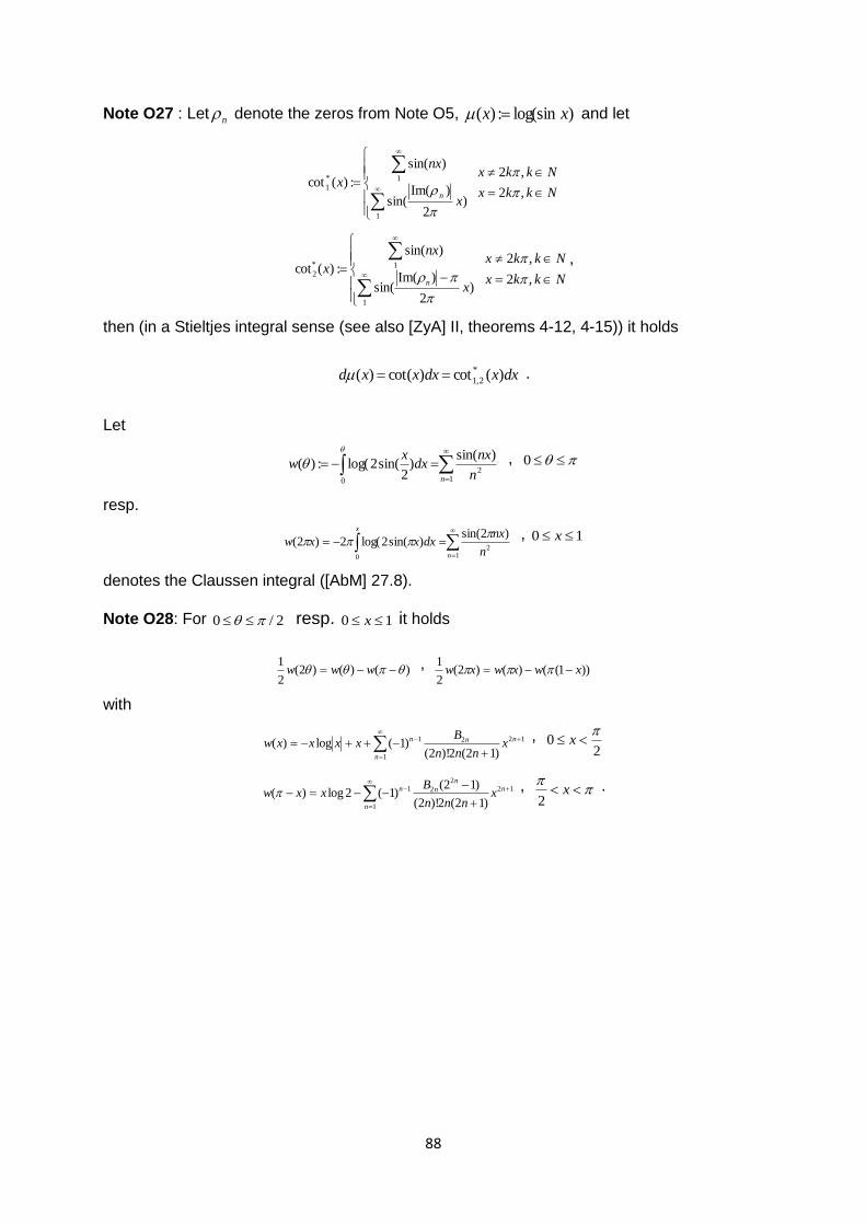
88
Note O27 : Let n denote the zeros from Note O5, )log(sin:)( xx and let
Nkkx
Nkkx
x
nx
xn
,2
,2
)2
)Im(sin(
)sin(
:)(cot
1
1*
1
Nkkx
Nkkx
x
nx
xn
,2
,2
)2
)Im(sin(
)sin(
:)(cot
1
1*
2
,
then (in a Stieltjes integral sense (see also [ZyA] II, theorems 4-12, 4-15)) it holds
dxxdxxxd )(cot)cot()( *
2,1 .
Let
1
2
0
)sin()
2sin(2log(:)(
n n
nxdx
xw
, 0
resp.
1
2
0
)2sin()sin(2log(2)2(
n
x
n
nxdxxxw
, 10 x
denotes the Claussen integral ([AbM] 27.8).
Note O28: For 2/0 resp. 10 x it holds
)()()2(2
1 www , ))1(()()2(
2
1xwxwxw
with
1
1221
)12(2)!2()1(log)(
n
nnn xnnn
Bxxxxw
, 2
0
x
1
122
21
)12(2)!2(
)12()1(2log)(
n
nn
nn xnnn
Bxxw ,
x
2 .
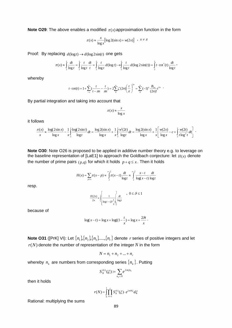
89
Note O29: The above enables a modified )(x approximation function in the form
)2()(sin2loglog
)( xwxx
xx , x
Proof: By replacing )sin(2(log)(log tdtd one gets
xxxxx
t
dttttd
t
ttd
t
t
t
dt
t
t
t
dtx
2
*
2222log
)(cot))sin(2(loglog
)(loglogloglog
)( ,
whereby
0
22
0
2
)!2()1()2(2)(1)cot( nnn
n
tn
Btn
n
t
nt
ttt
.
By partial integration and taking into account that
x
xx
log)(
it follows
xxx
dttt
twc
x
xw
xx
xdt
t
tw
xx
xdt
t
t
xx
x
x
x
2
2
22log
)2(
log
)2(1
log
)(sin2log
log
)2(1
log
)(sin2log
log
)sin2log(1
log
)sin2log()( .
Note O30: Note O26 is proposed to be applied in additive number theory e.g. to leverage on the baseline representation of [LaE1] to approach the Goldbach conjecture: let )(xH denote
the number of prime pairs ),( qp for which it holds xqp . Then it holds
2
2
2
2log)log(log
)()()(
x
xp
x
t
dt
tx
tx
t
dttxpxxH
resp.
x
t
dt
x
tt
x
xH
2log
)(log
1
2
)2(
, 10
because of
x
tx
x
txtx
2log)1log((log)log( .
Note O31 ([PrK] VI): Let rnnnn .....,,, 321 denote r series of positive integers and let
)(Nr denote the number of representation of the integer N in the form
rnnnN ...21
whereby kn are numbers from corresponding series kn . Putting
Nn
nik
N
k
keS 2)( :)(
then it holds
deSNr iNr
k
k
N
2
1
0 1
)( )()(
Rational: multiplying the sums
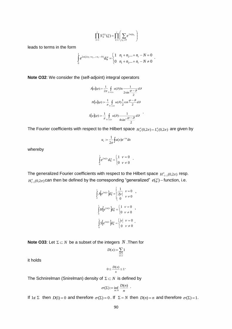
90
r
k Nn
nir
k
k
N
k
keS1
2
1
)( )(
leads to terms in the form
0...
0...
0
1
21
211
0
)...(2 21
Nnnn
Nnnnde
r
rNnnni r .
Note O32: We consider the (self-adjoint) integral operators
20
2sin2
1ln)(
2
1:)( duuA
duuH2
cot2
1)(
1:)(
20
20 2
2sin4
1)(
1:)( duuS
.
The Fourier coefficients with respect to the Hilbert space )2,0()2,0( #
2
#
0 LH are given by
dxexuu xi
)(2
1:
whereby
0
0
0
11
0
2
de i .
The generalized Fourier coefficients with respect to the Hilbert space )2,0(#
2/1 H resp.
)2,0(#
2/1 H can then be defined by the corresponding “generalized” )(e function, i.e.
0
0
0
2
11
0
2
deA i ,
0
0
0
11
0
2
deH i ,
0
0
0
1
0
2
deS i .
Note O33: Let N be a subset of the integers N .Then for
xaa
xD 1:)(
it holds
1)(
0 x
xD .
The Schnirelman (Snirelman) density of N is defined by
n
nD
Nn
)(inf:)(
.
If 1 then 0)1( D and therefore 0)( . If N then nnD )( and therefore 1)( .
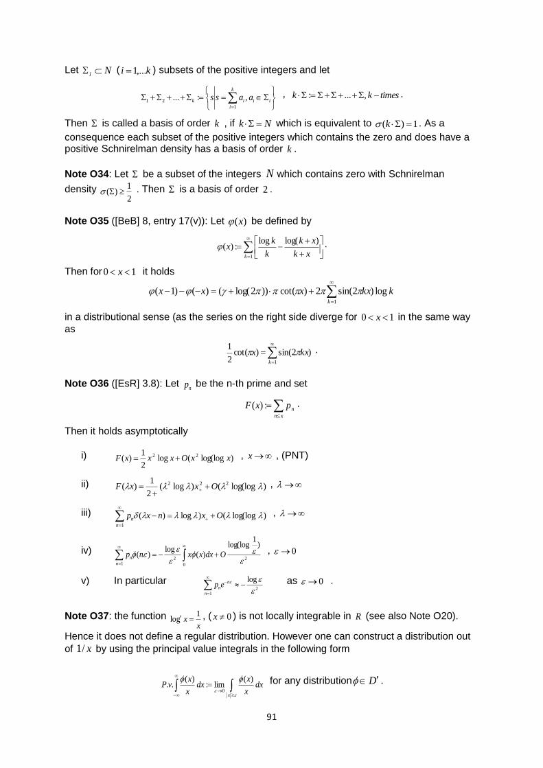
91
Let Ni ( ki ,...1 ) subsets of the positive integers and let
ii
k
i
ik aass ,:...1
21 , timeskk ,...: .
Then is called a basis of order k , if Nk which is equivalent to 1)( k . As a
consequence each subset of the positive integers which contains the zero and does have a positive Schnirelman density has a basis of order k .
Note O34: Let be a subset of the integers N which contains zero with Schnirelman
density 2
1)( . Then is a basis of order 2 .
Note O35 ([BeB] 8, entry 17(v)): Let )(x be defined by
1
)log(log:)(
k xk
xk
k
kx .
Then for 10 x it holds
1
log)2sin(2)cot())2log(()()1(k
kkxxxx
in a distributional sense (as the series on the right side diverge for 10 x in the same way
as
1
)2sin()cot(2
1
k
kxx .
Note O36 ([EsR] 3.8): Let
np be the n-th prime and set
xn
npxF :)( .
Then it holds asymptotically
i) )log(log(log2
1)( 22 xxOxxxF , x , (PNT)
ii) )log(log()log(2
1)( 222 OxxF
,
iii)
1
)log(log()log)(n
n Oxnxp ,
iv)
1 0
22
)1
log(log
)(log
)(n
n Odxxxnp
, 0
v) In particular
1
2
log
n
n
nep
as 0 .
Note O37: the function x
x1
glo , ( 0x ) is not locally integrable in R (see also Note O20).
Hence it does not define a regular distribution. However one can construct a distribution out
of x/1 by using the principal value integrals in the following form
x
dxx
xdx
x
xvP
)(lim:
)(..
0
for any distribution D .
92
Alternatively to the above we propose for 10 x in a distributional sense
1
* )2sin()(cot2
1
k
k xx
where k denotes the zeros of the hypergeometric confluent function in scope (e.g. Note
O5). The circle method applies the identity
0
0
0
11
0
2
n
ndxe inx
resp.
0,
0,1)sin(
2
0
nnm
nmnm
idxnxe imx
0
0
2
0
)cos(
2
0 nm
nm
nm
dxnxe imx
.
Its relationship to the zeros of the sin/cos-function is given by
xixe ix sincos .
Its counterpart with respect to the hypergeometric confluent function in scope and its related zeros is enabled by the Fresnel Integrals
))2
cos(:)(0
2
z
dttzC ,
))2
sin(:)(0
2
z
dttzS
and its relationship to the Dawson function
);2
3;1()( 11 xFxxF .
Note O38 ([AbM] 7.1.21, 7.3.25): It holds
)2
;2
3;
2
1()
2;
2
3;
2
1()()( 2
1122
11
2
ziFzeziFzziSzCzi
,
2
1)()( SC
resp.
)2;2
3;
2
1(2)2;
2
3;
2
1()2()2( 11
2
11 ixFexixFzxiSxC ix
resp.
)2
;2
3;
2
1(
)()( 2
11 ziFz
ziSzC
, )2
;2
3;
2
1(
)()( 2
11 ziFz
ziSzC
.
We further note that the set of zeros
Nnn ,0 contains the zero.
Note O39 ([OlF] 3): The asymptotic expansion of the Fresnel integrals are given by
0 )2(
)12(...3121
22
1)
2()
2(
nn
ix
ix
ne
x
ixiS
xC
x .
When 0x and 1n , the nth implied constant of this expansion does not exceed twice the
absolute value of the coefficient of the thn )1( term.
([GrI] 6.264):
0
2/log)( xdxxC .
93
We recall the series representation
1
)2
log(sin()cos(
n
x
n
nx ,
1
)(2
1)sin(
n
xn
nx , 20 x .
Note O20 indicates a distribution density function in the form )cot()(2 xxd . In this context
we recall Clausen’s integral and related summations: Note O40: Because of the orthogonality relations
0)sin()sin(
1
0
dxxmxn for mn
and, for the Bessel functions J and their nth zeros nj ,
0)()(
1
0
dxxjJxjxJ nn
those functions are called orthogonal with respect to their own zeros ([HaG1]).
Recalling Remark 1.5 ([TiE] 2.7) the self-reciprocal property for the sine transforms of
0
2)sin()(
2
2
1
1
1:)( dyxyyg
xexg
x
is applied for the fourth method to prove the Riemann duality equation. In the context of the above with respect to the confluent hypergeometric functions in scope of this paper we note Note O41 ([GrI] 7.663):
i) )
2;
2
3,1()()
2;
2
3,1(
2
11
0
1
2
11
yFdxxyJ
xFx
ii) )
4(
1
2)()
2;
2
3,
2
1(
2
0
0
41
2
11
2
yIe
ydxxyJ
xFx
y
iii) )
4(
2
1)()
2;
2
3,1(
2
0
0
40
2
11
2
yKedxxyJ
xFx
y
.
Note O42: From [LaE] §83, we recall
)1(glo)1(glo)
)2
sin(2
()( 2 ss
s
s
whereby
2
1)cosh(
2
1)
2(sinh)
2(cosh
2
1))
2
1(
2(sin 222
tttit
resp.
)(sec2
)
)2
sin(2
(2
2 th
s
.
94
Note O43 ([LuB], [LaE] §83): A )sin(2log( x function related Zeta function representation is
given by
)(log))1(
)2
sin(2
)1((glo)(glo tos
s
ss
resp. on the critical line
)
)2
1(
)sinh()cosh(2(glo)
)2
1(
)sin()cos(2(glo)
)1(
)2
sin(2
(glo)2
1(glo
2
it
tit
it
titi
s
s
it
for its with 2/1 , 0 fixed; the related Riemann duality equation is given by
([TiE] (2.1.9)
)1()1()2
sin()2(
)( sssss
From ([AbM] 6.1.32 we recall
)4
3()
4
1(
2
1
))sinh()(cosh(2
1ixix
xix
.
The linkage to the hypergeometric confluent functions can be built via the Hilbert transform applied to the identities ([GrI] 1.232), 0x
0
)12()1(2)cosh(
1
k
xkk ex
,
1
2)1(21)tanh(k
kxk ex .
The secans hyperbolicus function
022
2
4)12(
)12()1(4)
2
1(
)cosh()(sec
k
k
xk
kix
xxh
( x
ixix
x
)1()1(
)sinh(
)
defines a distribution similar to the normal distribution; the corresponding density function is given by
dtt
x
x
)cosh(
1:)(
with ([GrI] 3.511)
1)cosh(
1
dtt
.
From ([GrI] 2.423, we recall
))h(arcsin(tan)arctan(2))h(arctan(sin)cosh(
xexx
dx x
1cosh
1coshlog
2
1))
2log(tanh(
)sinh(
x
xx
x
dx .
95
Note O44 ([LaE] §56): The following two series are convergent and do have the same limit, which is the Euler constant,.i.e.,
xp
x
x
nx p
pxx
n 1
logloglimlog
1lim
1
From ([GrI] 2.477, we recall ( nE Euler constants)
0
12
2
)!2)(12()cosh( k
k
k
kk
xE
x
dx , 2
x .
We further note the equalities ([GrI] 3.511, 3.522)
0
)2
,2
1(
2
1
)(cosh
)(sinh
Bdxx
x 0)Re(,1)Re( .
from which is follows
0
)2
1,
2(
2
1
sinh
ssB
t
dts
1)Re(0 s
0
)2
1,
2
1(
2
1
)cosh(
)(sinh
Bdxx
x 1)Re( .
Note O45 ([BeB] 9. Entry 16): For 2/x ,
12
022
12 )2sin(
2
1sin2log
)12(2
sin2
nnn
n
n
nxxx
n
x
n
n .
Note O46 ([BeB] 5, Corollary 4 For 1)Re( s
1
0
)
)2
sin(
1()12(
)1(
ps
ks
k
p
s
k
from which it follows that the series
p p
p)2
sin(
converges. With respect to the properties of the Dawson function (lemmata D1-D4) we recall from [LaE] § 27, the
Note O47: let )(xf be a positive, not increasing function for 2x with 0)( f . Then
Adttfnfn
x
x
2 2
)()(lim
exists, and particularly it holds
))(()()(2 2
xfOAdttfnfn
x
.
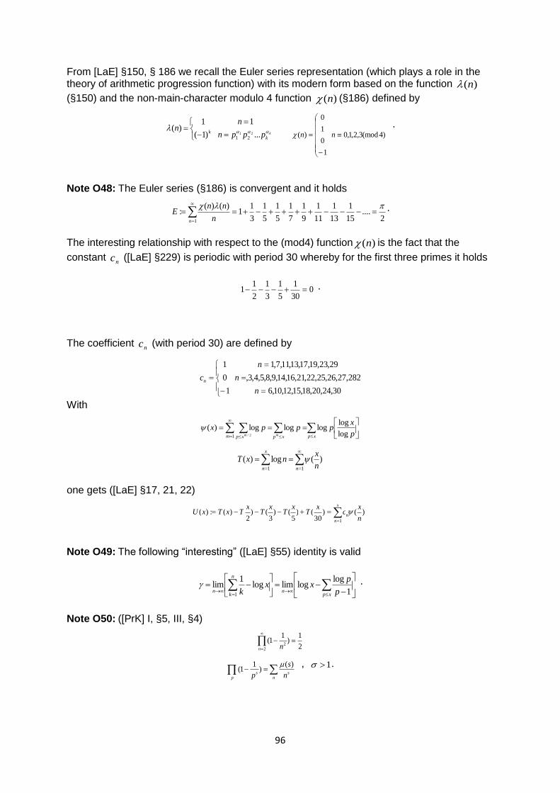
96
From [LaE] §150, § 186 we recall the Euler series representation (which plays a role in the theory of arithmetic progression function) with its modern form based on the function )(n
(§150) and the non-main-character modulo 4 function )(n (§186) defined by
k
k
k pppn
nn
...
1
)1(
1)(
21
21
)4(mod3,2,1,0
1
0
1
0
)(
nn
.
Note O48: The Euler series (§186) is convergent and it holds
1 2
....15
1
13
1
11
1
9
1
7
1
5
1
5
1
3
11
)()(:
n n
nnE
.
The interesting relationship with respect to the (mod4) function )(n is the fact that the
constant nc ([LaE] §229) is periodic with period 30 whereby for the first three primes it holds
030
1
5
1
3
1
2
11 .
The coefficient nc (with period 30) are defined by
30,24,20,18,15,12,10,6
282,27,26,25,22,21,16,14,9,8,5,4,3,
29,23,19,17,13,11,7,1
1
0
1
n
n
n
cn
With
xpxpm xp p
xpppx
mm log
loglogloglog)(
1 2/
11
)(log)(n
x
n n
xnxT
one gets ([LaE] §17, 21, 22)
Note O49: The following “interesting” ([LaE] §55) identity is valid
xpn
n
kn p
pxx
k 1
logloglimlog
1lim
1
.
Note O50: ([PrK] I, §5, III, §4)
2
1)
11(
22
n n
n
sp
s n
s
p
)()
11(
, 1 .
x
n n
n x
c x T x
T x T x
T x T x U 1
) ( ) 30
( ) 5
( ) 3
( ) 2
) ( : ) (
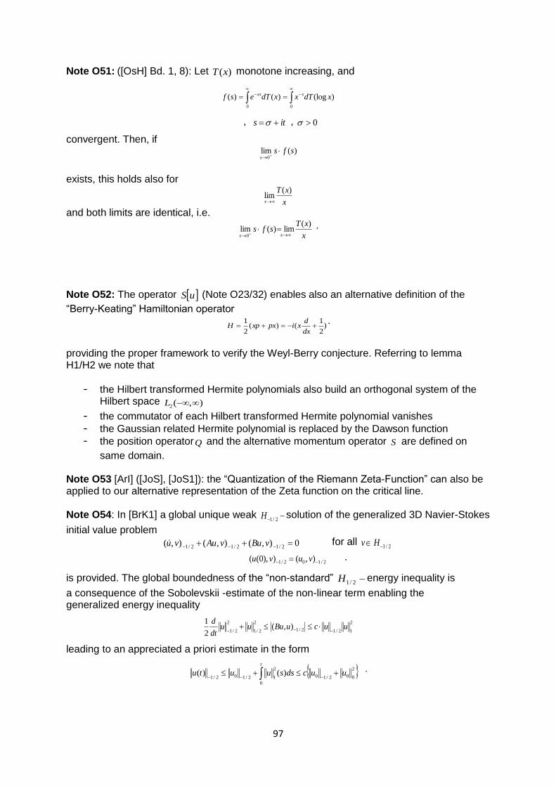
97
Note O51: ([OsH] Bd. 1, 8): Let )(xT monotone increasing, and
0 0
)(log)()( xdTxxdTesf ssx
, its , 0
convergent. Then, if )(lim
0
sfss
exists, this holds also for
x
xT
x
)(lim
and both limits are identical, i.e.
x
xTsfs
xs
)(lim)(lim
0
.
Note O52: The operator uS (Note O23/32) enables also an alternative definition of the
“Berry-Keating” Hamiltonian operator
)2
1()(
2
1
dx
dxipxxpH
.
providing the proper framework to verify the Weyl-Berry conjecture. Referring to lemma H1/H2 we note that
- the Hilbert transformed Hermite polynomials also build an orthogonal system of the Hilbert space ),(2 L
- the commutator of each Hilbert transformed Hermite polynomial vanishes
- the Gaussian related Hermite polynomial is replaced by the Dawson function
- the position operatorQ and the alternative momentum operator S are defined on
same domain. Note O53 [ArI] ([JoS], [JoS1]): the “Quantization of the Riemann Zeta-Function” can also be applied to our alternative representation of the Zeta function on the critical line. Note O54: In [BrK1] a global unique weak 2/1H solution of the generalized 3D Navier-Stokes
initial value problem 0),(),(),( 2/12/12/1 vBuvAuvu for all
2/1Hv
2/102/1 ),()),0(( vuvu .
is provided. The global boundedness of the “non-standard” 2/1H energy inequality is
a consequence of the Sobolevskii -estimate of the non-linear term enabling the generalized energy inequality
2
12/12/1
2
2/1
2
2/1),(
2
1uucuBuuu
dt
d
leading to an appreciated a priori estimate in the form
2
002/10
0
2
12/102/1)()( uucdssuutu
t
.
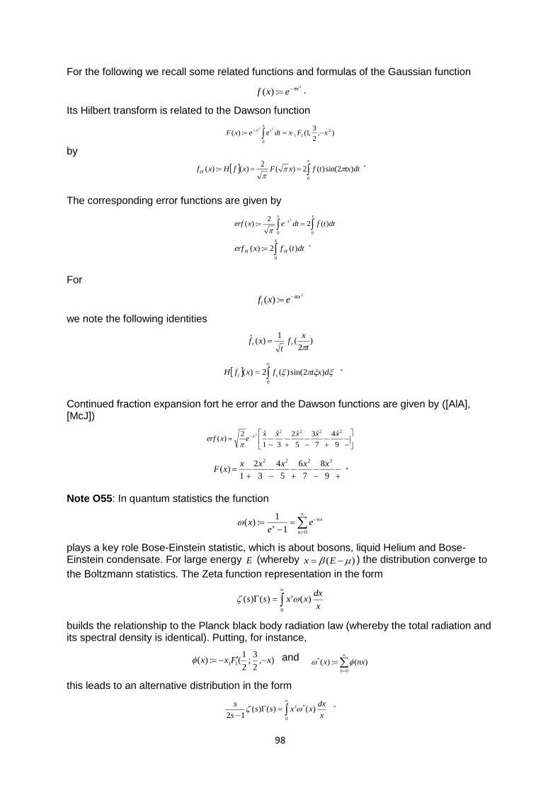
98
For the following we recall some related functions and formulas of the Gaussian function
2
:)( xexf .
Its Hilbert transform is related to the Dawson function
),2
3,1(:)( 2
11
0
22
xFxdteexF
x
tx
by
0
)2sin()(2)(2
)(:)( dttxtfxFxfHxf H
.
The corresponding error functions are given by
xx
t dttfdtexerf00
)(22
:)(2
x
HH dttfxerf0
)(2:)( .
For
2
:)( tx
t exf
we note the following identities
)2
(1
)(ˆt
xf
txf tt
0
)2sin()(2)( dxtfxfH tt
.
Continued fraction expansion fort he error and the Dawson functions are given by ([AlA], [McJ])
9
ˆ4
7
ˆ3
5
ˆ2
3
ˆ
1
ˆ2)(
22222 xxxxx
exerf x
9
8
7
6
5
4
3
2
1)(
2222 xxxxxxF .
Note O55: In quantum statistics the function
01
1:)(
n
nx
xe
ex
plays a key role Bose-Einstein statistic, which is about bosons, liquid Helium and Bose-Einstein condensate. For large energy E (whereby )( Ex ) the distribution converge to
the Boltzmann statistics. The Zeta function representation in the form
0
)()()(x
dxxxss s
builds the relationship to the Planck black body radiation law (whereby the total radiation and its spectral density is identical). Putting, for instance,
),2
3;
2
1(:)( 11 xFxx and
0
* )(:)(n
nxx
this leads to an alternative distribution in the form
0
* )()()(12 x
dxxxss
s
s s .
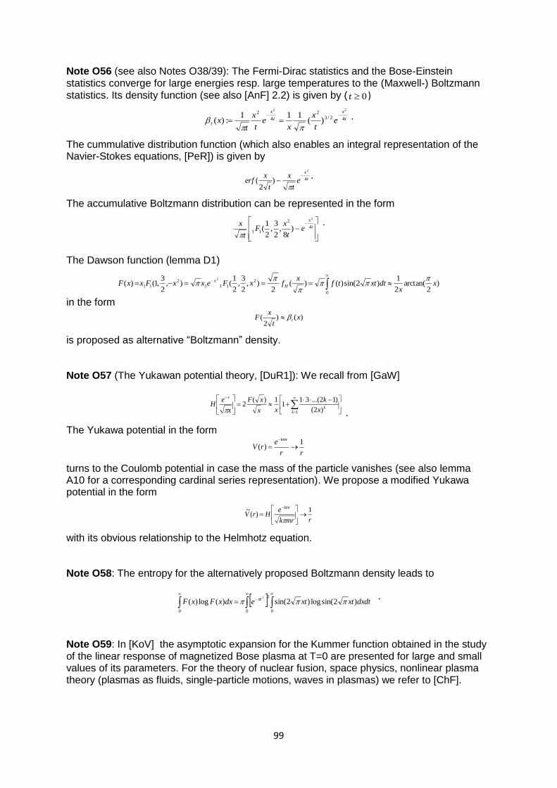
99
Note O56 (see also Notes O38/39): The Fermi-Dirac statistics and the Bose-Einstein statistics converge for large energies resp. large temperatures to the (Maxwell-) Boltzmann statistics. Its density function (see also [AnF] 2.2) is given by ( 0t )
t
x
t
x
t et
x
xe
t
x
tx 42/3
2
4
222
)(111
:)(
.
The cummulative distribution function (which also enables an integral representation of the Navier-Stokes equations, [PeR]) is given by
t
x
et
x
t
xerf 4
2
)2
(
.
The accumulative Boltzmann distribution can be represented in the form
t
x
et
xF
t
x4
2
11
2
)8
,2
3,
2
1(
.
The Dawson function (lemma D1)
)2
arctan(2
1)2sin()()(
2),
2
3,
2
1(),
2
3,1()(
0
2
111
2
11
2
xx
dtxttfx
fxFexxFxxF H
x
in the form
)()2
( xt
xF t
is proposed as alternative “Boltzmann” density. Note O57 (The Yukawan potential theory, [DuR1]): We recall from [GaW]
1 )2(
)12...(311
1)(2
kk
x
x
k
xx
xF
x
eH
.
The Yukawa potential in the form
rr
erV
kmr 1)(
turns to the Coulomb potential in case the mass of the particle vanishes (see also lemma A10 for a corresponding cardinal series representation). We propose a modified Yukawa potential in the form
rmrk
eHrV
kmr 1)(
~
with its obvious relationship to the Helmhotz equation. Note O58: The entropy for the alternatively proposed Boltzmann density leads to
0 0
2
0
)2sin(log)2sin()(log)(2
dxdtxtxtedxxFxF t .
Note O59: In [KoV] the asymptotic expansion for the Kummer function obtained in the study of the linear response of magnetized Bose plasma at T=0 are presented for large and small values of its parameters. For the theory of nuclear fusion, space physics, nonlinear plasma theory (plasmas as fluids, single-particle motions, waves in plasmas) we refer to [ChF].
100
Note O60: Dispersion relation/Landau damping for/of the transverse electromagnetic wave; the Plasma dispersion function (which is identical to the Dawson function) ([ChF] 7.9.1, [BiJ] 5.3, 5.4):
The Vlasov equation is used to derive the dispersion relation for electron plasma oscillations. In zeroth order one assumes a uniform plasma with distribution )(0 vf . In first order, one
denotes the perturbation ),,( tvrf by ),,(1 tvrf in the form
),,()(),,( 10 tvrfvftvrf
The plasma dispersion function )(Z defined by
ds
s
eZ
s
2
1)(
, 0)( mI
is applied to calculate the ion Landau damping of ion acoustic waves in the absence of magnetic fields. It is derived from the solution
j
jj
j
j
jkv
vf
m
Eiqf
/0
1
(the jth species has charge jq , mass
jm , and particle velocityjv ) of the Vlasov equation.
The density perturbation of the jth species is given by
j
j
jj
j
j
jjjij dvkv
vf
m
Eiqdvvfn
/)(
0
1 .
Setting 2/1
0
22
0 )/( jjjpj MeZn
one gets the dispersion relation
j jthj
pj
e
the
p
ZvZ
vk
)()(
2
2
2
2
2
from which electron plasma waves can be obtained setting 0 pj (infinitely massive ions).
Putting 22
2
2 12:
Dthe
p
Dv
k
, )/(: thjj kv
one obtains
)(2
12
2
e
D
Zk
k
,
which is the same as ([BiJ] (6.2)):
dvkv
vf
k
ep
)/(
/1 0
2
2
when ef 0 is Maxwellian. The term 22
Dk represents the deviation from quasineutrality. For
the special case of a single ion species ( 122 Dk ) the dispersion relation becomes
e
i
thi ZT
T
kvZ
2)(
.
“Solving this equation is a nontrivial problem” ([ChF] (7.128)). Considering the limit 1j the
asymptotic expression ....
2
32)( 42
2
iiiiieiZ
is applied to calculate the approximate damping rate. For an alternative calculation procedure we recall the relationship of the Dawson function and its first derivative ([GrI] 3.896, 3.952) given by
),2
3,1()2sin( 2
11
0
2
xFxdtxte t
, 22
2
1)2cos(
0
xt edtxte
),2
1,1()2cos(2 2
11
0
2
xFdtxtet t
.
101
Note O61: The Boltzmann equation with Maxwellian (Gaussian) molecules is given by
),)(,(),( vtffQvtt
f
with the non-linear collision operator ),( ffQ . The Boltzmann's equation is a nonlinear
integro-differential equation with a linear first-order operator. The nonlinearity comes from the quadratic integral (collision) operator that is decomposed into two parts (usually called the gain and the loss terms). In [LiP] it is proven that the gain term enjoys striking compactness properties. The Fokker-Planck (Landau) equation is given by
),)(,(),(),( vtffQvtfvvtt
fx
.
Analog to ([BrK1]) we propose a variational representation in the form
2/12/12/1 ),()),,((),( vfQgvfvgf x for all
2/1Hg .
The existence of global solutions of the Boltzmann and Landau equations depends heavily on the structure of the collision operators ([LiP1]). The corresponding variational
representation of KAB with a H coercive operator A and a compact disturbance K
fulfills a Garding type inequality in the form (see also [KaY])
),(),( vKuvucvBu
or 2
2
2
1),(
ucucvBu
with HH compactly embedded.
The Boltzmann equation and the Fokker-Planck (Landau) equation are concerned with the Kullback information, which is about a differential entropy defined by
dxxh
xhXH)(
1log)()(
.
It plays a key role in the mathematical expression of the entropy principle. The Boltzmann entropy is given by
hdvdxhS log .
The regularity of the solution(s) of the Landau equation heavily depends from the differential entropy is essential. We note that ([GrI] 4.384)
1
0
)2log1(4
)sin()log(sin
dxxx .
102
Note O62 The Boltzmann equation, complicated structure of the collision integral replaced by BGK (Bhatnagar-Gross-Krook) collision model, ([CeC] II, 10):
One of the major shortcomings in dealing with the Boltzmann equation is the complicated structure of the collision integral. The idea behind a replacement by a collision (kinetic) model is that a large amout of detail of the two-body interaction is not likely to influence significantly the values of many experimentally measured quantities. That is that the fine structure of the collision operator ),( ffQ can be replaced by a blurred image, based upon a simpler
operator )( fJ , which retains only the qualitative and average properties of the true collision
operator. The most widely known collision model is usually called the BGK model. The idea behind the BGK model is that the essential features of a collision operator are: the collison model must satisfy
i) 0)( dfJ , 4,3,2,1,0 , collision invariants
ii) 0)(log dfJf (with equality holding iff is a Maxwellian).
The second property expresses the tendency of the gas to a Maxwellian distribution. The simplest way of taking this feature into account seems to assume that the average effect of collisions is the change the distribution function )(f by an amount proportional to the
departure of f from a Maxwellian )( . so, if is a constant with respect to , we
introduce the following collision model
)()(:)( ffJ .
The Maxwellian )( has five disposable scalar parameters ),,( Tv according to the
equations
2)()( veAf
11 )2()4(3 RTe , 2
3
2
3
)2()3
4(
RTeA .
The BGK model satisfy ii) and quality applies iff is a Maxwellian. The nonlinearity of )( fJ is much worse than the nonlinearity of the collision term. In fact the
latter is simply quadratic in f , while the former contains f in both the numerator and the
denominator of an exponential (the and T appearing in are functionals of f ). In other
words, the collision term can be interpreted as a compact disturbance of the )( fJ model.
The main advantage in using the BGK model collision term is that for any given problem one can deduce integral equations for the macroscopic variables Tv,, .
If P is a probability density ( 1Pd ), then
PdPPPH loglog)(
(where d is the volume element in the space M of the events, whose probability density is
P ) is a suitable measure of the likelihood of P . In other words, if we take several sP' “at
random”, provided positive and normalized, most of them will be close to the probability density P for which )(PH is minimum.
The latter one enables variational theory concepts. In ([CeC] IV, 10, linear transport) a variational principle for the linerarized Boltzmann equation is provided, based on an appropriately defined self-adjoint operator with respect to a certain scalar product.
103
Note O63 The Hilbert transform applied to a nonlocal transport equation:
For 10 inner products are defined by ([CoA])
0)()((:)),((2
x
dxxvxuxvu
for even )(1 RHu
0))(()(:)),((2
x
dxxvxuxvu H
for even )(1 RHu .
Then the central a priori estimates are given by ([CoA], theorem 1.1/1.4)
A. For )()( 11 RHRCf and
A1: 10 , f even, it holds
dxx
xfxfcdx
x
fxf H
221
2 )()())0()((
A2: 12/1 and f nonnegative (or nonpositive), it holds
dxx
xfxfcdx
x
fxf H
221
2 )()())0()((
B. For )()( 11 RHRCf and
B1: For 10 , f even, it holds
dxx
xfxfcdx
x
xf H
221
2 )()()(
B2: For 12/1 , f nonnegative (or nonpositive), it holds
dxx
xfxfcdx
x
xf H
221
2 )()()( .
Note O64 Reduced (semi-infinite & finite) Hilbert transform, Stieltjes integral, Plemelj formula, diagonalizing operator ([ShE]): The Hilbert transform operator
dyxy
yu
ixuH
)(1:)(
acting on functions ),(2 Lu defines an unitary, symmetric operator on ),(2 L . Its
spectrum consists just of the points 1 . Hilbert tranforms on R are defined by ( 0x )
dy
xiy
yu
ixuH
)(
2
1lim:)(
0
.
By Plemelj’s formulas we have the relations
uHu
uH 2
.
For ),( t , )2/1,2/1( and
0
2
1
)(:)(x
dxxxutuM
it , 1
)2
1(2
1:)(
iti
et
.
it holds for certain (fastly decreasing) functions ([ShE] Theorem 1.1, see also lemma H2)
)()( xxHxxH i.e. 0)( xxHHx
where
MH , MMH )1(
yielding a spectral decomposition of the isometry M ([ShE] Remark 1.2).
104
Note O65 (The Landau damping, optimal transport, integral inequalities for the Hilbert transform applied to a nonlocal (Burgers type) transport equation in one space variable): The Vlasov-Poisson equation (the collisionless Boltzmann equation) is time-reversible (due to the Landau damping, [MoC]). Landau predicted this irreversible behavior on the analysis of the solution of the Cauchy problem for the linearized Vlasov equation around a spacially homogeneous Maxwellian (Gaussian) equilibrium. Landau formally solved the equation by means of Fourier and Laplace transforms. This phenomenon prevents an instability from developing, and creates a region of stability in the parameter space. In [GlR], [GlR1], it is shown that a solution of the linearized Vlasov equation in the whole space (linearized around a homogeneous equilibrium )0(:0 ff of infinite mass) decays at
best like modulo logarithmic corrections, for 1
0 )21()( vcvf ; and like )(log tO if 0f is
a Gaussian. In order to get an answer to the question, if convergence holds in infinite time for the solution of the “full” nonlinear equation there is a mechanism required that would keep
the distribution function f close to the original equilibrium.
This note is about a new proposed Landau theory, based on (distributional Hilbert scale) functional spaces and related functional inequalities for the nonlinear transport equation, alternatively to the approach in [MoC] establishing exponential Laundau damping in analytical regularity built on analytical norms having up to 5 parameters (which is far away from any physical meaning).Our alternative approach is based on the results of [CoA], incorporating the Hilbert transform concept to define appropriate Hilbert space norms. The Galerkin-Ritz method is proposed to calculate corresponding (quasi-optimal) approximation solutions, e.g. with underlying boundary elements approximation spaces or trigonometric functions approximation spaces ([BrK]). We note that the Hilbert transform is also applied in [DeP] for a spectral theory of the linearized Vlasov-poisson equation. In [CoA] the existence of finite-time singularities for a Burgers type equation
0 fff H
with nonlocal velocity in one space variable is shown. The motivation for the study of that equation is its analogy for the 3D Euler equation in vorticy form, having its origin in the CLM-model (Constatin-Lax-Majda), see also [BrK1]). The proposed function space )(1 RH
, , is th
closure of )(1
0 RC under the norm
dxx
xfdx
x
fxfff
L
12
2
12
222 )(())0()((
, 10 .
It is straightforward to obtain the following a priori estimate
2/32
0
2
0
2
0
2
0ffcff
dt
d
which implies local (in time) existence of the Cauchy problem with initial data in Sobolev space )(1 RH , which also cannot be justified by corresponding physical
requirements/meanings. We note that in the one-dimensional case the Sobolev embedding theorem state that
0CH k for 2/2/1 nk .
The above is about a particle dynamics given by the ordinary differential equation
)),(()( ttXftX H
and the equation implies that f is constant along the trajectories.
105
If one changes coordinates to a system of reference in which the maximum is stationary, i.e. if one defines )(txM
to be the trajectory where f reaches its maximum, and
)(txxy M , t
one obtaines from the equation above the equation
0),()( yHyM fyfftxf
resp.
0))0()(( yHH ffyff
where
)),((),( ttxyfyf M .
Note O66 ([BuP], p. 20) Theorem of Privalov:
For )1,0( let )(Lipf be a periodic function, then )(LipfH .
Note O67 ([GaG]): The Laguerre polynomials
),1,(!
)1()( 11 xnF
nxL n
n
satisfy the orthogonality relation ( 1 )
mn
x
mnn
ndxexxLxL ,
0!
)1()()(
, ,...2,1,0, mn .
Note O68 Reduced finite Hilbert transform operator, Schrödinger differential operator, ([KoW]): The finite Hilbert transform operators
b
a
ba dyxy
yu
ixuT
)(1:)(),(
, ba , bxa
are bounded in ),(2 baL with norm 1),( baT . The self-adjoint Schrödinger differential operator
dx
di defined for ),(2 Lu is isometrically equivalent to
))(())((1
:),( xbaxidx
dxbaxi
iD ba
, ),(2 baLg
which is isometrically equivalent to the multiplicative operator
),(
),(
1
1log
2)()
1
1log
2(:)(
ba
ba
T
Tabg
abgQ
,
defined for all )1,1(2 Lg such that
1
1
2
)(1
1log
dg
.
106
Note O69 (Alternative modelling concept for the Landau damping): We propose to apply the distributional Hilbert space concept of this paper (see also Note O53) to derive model adequate a priori estimate for the transport equation. The objective is, that the appropriately defined (distributional Hilbert space) norms enable appropriate Landau damping estimates, based on “realistic” physical modelling assumptions:
Following the ideas from [BrK1] [BrK3] this first leads to a change from
2
0
2
0
22
)0(: f
x
fff
L
to
2
2/1
2
0
22
2/1
2
2/1
22
)2/1(: f
x
fff
x
fff
LL
.
Anticipating the results from O60/61 (while at the same time also anticipating a “correct” balance between the Hilbert-space norm and a related Hölder norm, which is the appropriate norm to model nonlinear Partial Differential or PDO equations) we suggest the slightly “weaker” norm
22
0
22
.0:
ffxff
C ,
)2
1,
2
1(
and an analysis of a weak )2/1(H Hilbert transformed Fourier-Hermite wavelet of the
Vlasov solution enabled by Hilbert transformed Hermite polynomials,
)()( xHAxHH nn
which also build an orthogonal basis of ),(2 L (Definitions H1-H2, Lemma H1). Below we
proposed Morlet wavelet below for the Gaussian function
2
:)( tx
t exf
we recall the Fourier and Hilbert transform for the Gaussian function
)2
(1
)(ˆt
xf
txf tt
,
0
)2sin()(2)( dxtfxfH tt
.
With respect to Hölder regularity and fractional diffusion transport equation we refer to [ChD]. Note O70 Plasma is the fourth state of matter, where from general relativity and quantum theory its known that all of them are fakes resp. interim specific mathematical model items. Plasma is an ionized gas consisting of approximately equal numbers of positively charged ions and negatively charged charged electrons. One of the key differentiator to neutral gas is the fact that its electrically charged particles are strongly influenced by electric and magnetic fields, while neutral gas are not. As a consequence the quantitative fluid/gas behavior as it is described by the Euler or the Navier-Stokes equations can not be applied as adequate mathematical model. Even hi would be possible there is no linkage to the quantitative fluid/gas/plasma behavior and its corresponding turbulence behavior as it is described by the Euler or the Navier-Stokes equations.The approach in statistical turbulence is about low- and high-pass filtering Fourier coefficients analysis which is about a “local Fourier spectrum” analysis. As pointed out in [FaM] this is a contradiction in itself, as, either it is non-Fourier, or it is nonlocal. The proposal in [BrK1] is about a combination of the wavelet based solution concept of [FaM], [FaM1], with a revisited CLM equation model in a physical 2/1H Hilbert
space framework. The intension is, that this approach enables a turbulent 2/1H signal which
can be split into two components: coherent bursts and incoherent noise. Additionally the model enables a localized Heisenberg uncertainty inequality in the closed (“noise”/”wave packages”) subspace
02/1 HH , while the momentum-location commutator vanishes in the
(coherent bursts) test space 0H . As a first trial we propose the Morlet wavelet, which is a sin
wave that is windowed (i.e. mulitiplied point by point) by a Gaussian, having a mean value of zero.
107
We recall a few central symbols/formulas/equalities:
2/2/1 2
)2()( vevF Maxwellian velocity distribution
E electric density
)(xf distribution function of electrons
)0(ˆ0 ff Fourier transform of initial perturbance in )(xf
)( fC collision term (functional of f )
H Hermite polynomials of order
n electron density, Fourier-Laplace transform of electron density
The ordinary one-dimensional Boltzmann equation (in natural units) for the single-particle
distribution function )(xf of the electrons is given by
)( fCv
fE
x
fv
t
f
1fdv
x
E .
The Fourier-Hermite expansion is given by
2/2
)(2
1)( vkxi evHeaxf
where 2/2/ 22
)()1()( vv edv
devH
and
!)()(2
1 2/2
ndvevHvH nm
v
mn
.
Note O71 Superconductivity, superfluids and condensates ([AnJ]):
A superconductor is a charged fluid, which is a Bose-condensed state of interacting bosons. The degree of freedom of the Ginzburg-Landau theory (varying smoothly in space) are two fields
- complex-valued „order parameter“ field )()()( rierr , defining superconducring
order, as a fuction of the “superfluid density )(rns
and a complex phase angle )(r
- vector potential, representing the electromagnetic degress of freedom.
The existence of the “order parameter” is postulated by the GLAG theory. It characterizes the superconducting state, in the same way as the magnetization does in ferromagnet. It is assumed to be some (unspecific) physical quantity, which characterizes the state of the system. In the normal state above the critical temperature of the superconductor it is zero, below this state it is nonzero. Referring to the “rotating fluids” concept of [BrK1] (note O54), and, at the same time, in line with the alternative “ground state energy model of the harmonic quantum oscillator” in [BrK3], we propose (with test space
0H , state space 2/1H and energy space
2/1H )
)(:)( rPr
,
02/1: HHP , 2/1 H ,
0H , 0H
as an appropriately related “order parameter” projection operator. The closed space
2/10
HH could be interpreted as the “plasma (quantum) field” state space (where the
Heisenberg uncertainty inequality is valid), while 0H remains to be the “test space” of
(measurable) observations, governed by the two self-adjoint ladder operators ([AnJ] 5.2).
108
Note O72 Thermodynamics, Boltzmann relation and absolute zero ([FeE] 31):
A thermodynamical state of a system is not a sharply defined state of the system, because it corresponds to a lage number of dynamical states. This condieration led to the Boltzmann relation
pkS log
where p is the (infinite) number of dynamical states that correspond to the given
thermodynamical state. The value of p , and therefore the value of the entropy also,
depends on the arbitrarily chosen size of the cells by which the phase space is devided of which having the same hyper-volume . If the volume of the cells is made vanishing small,
both p and S become infinite. It can be shown, however, that if we change , p is altered
by a factor. But from the Boltzmann relation it follows that an undetermined factor in p gives
rise to an undetermined additive constant in S . Therefore the classical statistical mechanics
cannot lead to a determination of the entropy constant. This arbitrariness associated with p
can be removed by making use of the principles of quantum theory (providing discrete quantum state without making use of the arbitrary division of the phase space into cells).
Accoring to the Boltzmann relation, the value of p which corresponds to 0S is 1p .
Statistically interpreted, therefore, Nernst’s theorem (the third law of thermodynamics) states that “to the thermodynamical state of a system at absolute zero there corresponds only one dynamical state, namely, the dynamical state of lowest energy compatible with the given crystalline structure or state of aggregation of the system”.
Nerst’s theorem applied to solids leads to the entropy of the body at the temperature T in the form
T
dTT
TCS
0
)(
where the thermal capacity at absolute zero )0(C needs to be zero, otherwise the integral
would diverges.
The understanding that the zero state energy is uniquely determined is a miss understanding ([BrK3]). The value is just determined by the chosen mathematical model, i.e a purely mathematical requirement to ensure convergent series and integrals (note: the GRT requires differentiable manifolds, whereby only continuous manifolds ae required from a physical
modelling perspective). The Debye “temperature” constant for the specific heat of solids
elements is an example in the context of above, leading to the theoretical formula
)(3)(
TRDTC
We claim that as a consequence of the alternative harmonic quantum oscillator model (i.e. the alternative “plasma”/”wave package” state/energy spaces and corresponding continuous spectra) there is a challenge on the 3rd thermodynamical law:
“The entropy of every system at absolute zero can always be taken to zero”.
Only all orthogonal projection of those states (resp. the corresponding eigenvalues of the projection operator) onto the test space
0H are zero.
We propose an alternative entropy definition and a related closed absolute zero (Hilbert) state space in the form
2/1),()log,(:)( ppppph , 2/1,
0
H .
A revisit of the 3rd thermodynamical law would lead to a revisit of the Fermi-Dirac statistics; the Dawson function alternative above implies already a revisit of the Bose-Einstein statistics (represented by the function 1)1( xe ). It is predicted that both revisited statistics will become
integrated parts of an overall quantum gravity model ( www.quantum-gravitation.de ).
109
Fourier-Stieltjes integral, Cardinal series and the Claussen integral function For the following we refer to [WhJ] §11. The cardinal series are in a certain sense equivalent to the Newton-Gauss series (enabled by the method of de la Vallée Poussin). It is proposed to be an appropriate alternative to the Euler-Maclaurin summation (a technique for the numerical evaluation of sums introduced by Euler to compute )(n for Nn , [EdH] 5, 6) .
Let the series
(*)
1
0 )sin()cos(2
1
n
nn nxbnxaa
be called a Fourier-Stietjes series, if there is continuous function )(xF such that
)(1
0 xdFa ,
)()cos(1
xdFnxan
,
)()sin(1
xdFnxbn
.
The necessary and sufficient condition that (*) should be a Fourier-Stietjes series is that
1
)sin()cos(1
n
nn nxbnxan
should be a Fourier series of a continuous function )(xG , whereby the functions )(),( xGxF
being connected by the equation (see also Note O26)
xaxGxF 02
1)()( .
Assume that ,....,,,,..., 21012 aaaaa
is a sequence such that
(1)
1
1
n
nn aan
;
then
1
)sin(1
n
nn ntaan
,
1
)cos(1
n
nn ntaan
converge to continuous functions, so that there are continuous function )(),( tt such that
1
0
0 )(tda ,
1
0
)()cos(2
1tdntaa nn ,
1
0
)()sin(2
1tdntaa nn
whence, for all the values of n ,
(2)
1
0
)()sin()()cos( tdnttdntan .
We emphasis that
nn
S
vnuidguvuS1
),(
defines an inner product on *2/1
2
2/1
2 )( ll ([NaS], i.e. the generalized Fourier coefficients
nun are square summable; for functions with vanishing constant Fourier term the norm of
the corresponding dual space is given by
1
22
2/1
1nu
nu
110
A cardinal series then is defined by
(3)
1
0 )1(2
)sin(
n
nnn
nz
a
nz
aaz
.
Substituting the functions
1
11)cos()1(
1)sin(
n
n
nxnxnt
x
z
1
11)sin()1(
1)sin(
n
n
nxnxnt
x
z
in the integral of
(5)
1
0
)()sin()()cos()( tdnttdntxf
and then integrating term by term results into the (C,1)-summable series
(6) .
1
)()()1(
)0()sin(
n
n
nx
nf
nx
nf
x
fx
A cardinal series in the form (3) represent an entire function of order one. The cardinal series is particularly favored because the entire function )sin( z is orthogonal to its own zeros, i.e.
0)sin()sin(
1
0
dtmtnt , mn .
Theorem 16: Given a function )(xf of the form (5) the series (6) is (C,1)-summable and its
sum is )(xf . If (1) is satisfied, the cardinal series
(7)
1
0 )1()sin(
n
nnn
nx
a
nx
a
x
ax
is absolutely convergent and its sum is of the form (5). Theorem 17: If
(8)
1
log
n
nn aan
n
so that the cardinal series (7) is absolutely convergent, and is any real number,
n
n
nx
nCxxC
)()1(
))(sin()(
the series on the right being absolutely convergent. Moreover
1 2
110
log)()()(
1)(
n n
nn aan
naaaAnCnC
nC
where )(A depends only from .
Note that the proof of theorem 17 depends on the fact that )sin( z has an addition (!!)
theorem, and this property is not possesses by any other entire function, i.e. the so-called addition theorem for Bessel functions is not being an adequate substitute.
111
From [GrI] 4.384 we recall the appropriate Fourier-Stieltjes coefficients for the Claussen integral function. Let
)log(sin(:)( xxd 0:)( xd
then it holds
0
01
2log2
)()cos(
1
0
n
n
n
tdnt ,
1
0
0)()sin( tdnt
resp.
2log20 a , naa nn /1 .
The following is related to the corresponding Mellin inverse problem [NiN] Bd. 1, §89. The related orthogonal equations for the xsinlog and the )(log x functions are provided in
§78, related “discontinuous integrals” in the form
ndxxsixn
1)()cos(2
0
,
are provided in [NiN] Bd. 2, §21.
Given that )(xW has a representation in the form
1
0
1)()( dtttxW x .
Let
1
0)1(1
)(:)( dt
xt
txf
,
1
01
)(:)( dt
tx
txg
then there is a representation in the form
)()1()(sin
21 xVxVxWx
with
1
0
1
1 )()( dtttgxV x ,
1
0
1
21
)1
1(
)( dttt
tf
xV x
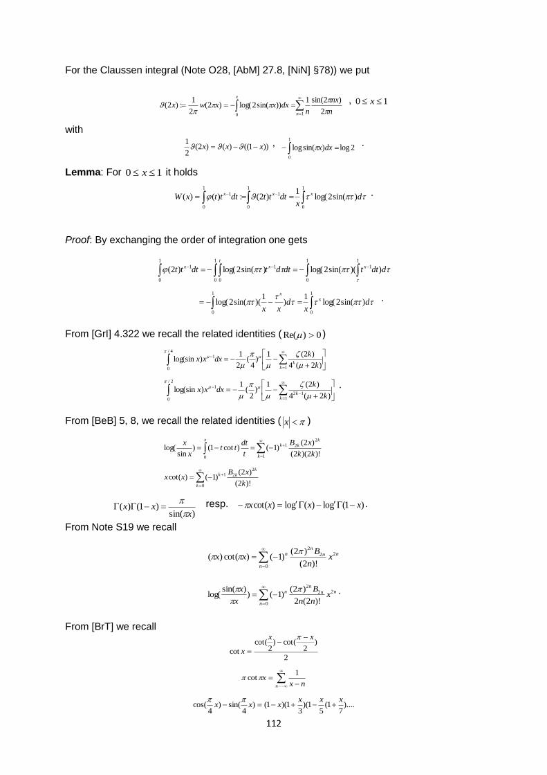
112
For the Claussen integral (Note O28, [AbM] 27.8, [NiN] §78)) we put
10
2
)2sin(1))sin(2log()2(
2
1:)2(
n
x
n
nx
ndxxxwx
, 10 x
with
))1(()()2(2
1xxx ,
2log)sin(log
1
0
dxx .
Lemma: For 10 x it holds
1
0
1
0
1
1
0
1 )sin(2log(1
)2(:)()( dx
dtttdtttxW xxx .
Proof: By exchanging the order of integration one gets
1
0
1
1
1
0
1
0
1
0
1 ))(sin(2log()sin(2log()2(
ddttdtdtdttt xx
t
x
1
0
1
0
)sin(2log(1
)1
)(sin(2log(
dx
dxx
xx
.
From [GrI] 4.322 we recall the related identities ( 0)Re( )
4/
0 1
1
)2(4
)2(1)
4(
2
1)log(sin
kk k
kdxxx
2/
0 112
1
)2(4
)2(1)
2(
1)log(sin
kk k
kdxxx
.
From [BeB] 5, 8, we recall the related identities ( x )
x
k
k
kk
kk
xB
t
dttt
x
x
0 1
2
21
)!2)(2(
)2()1()cot1()
sinlog(
0
2
21
)!2(
)2()1()cot(
k
k
kk
k
xBxx
)sin()1()(
xxx
resp. )1(glo)(glo)cot( xxxx .
From Note S19 we recall
0
22
2
)!2(
)2()1()cot()(
n
nn
nn x
n
Bxx
0
22
2
)!2(2
)2()1()
)sin(log(
n
nn
nn x
nn
B
x
x
.
From [BrT] we recall
2
)2
cot()2
cot(
cot
xx
x
n nxx
1cot
)....7
1(5
1)(3
1)(1()4
sin()4
cos(xxx
xxx
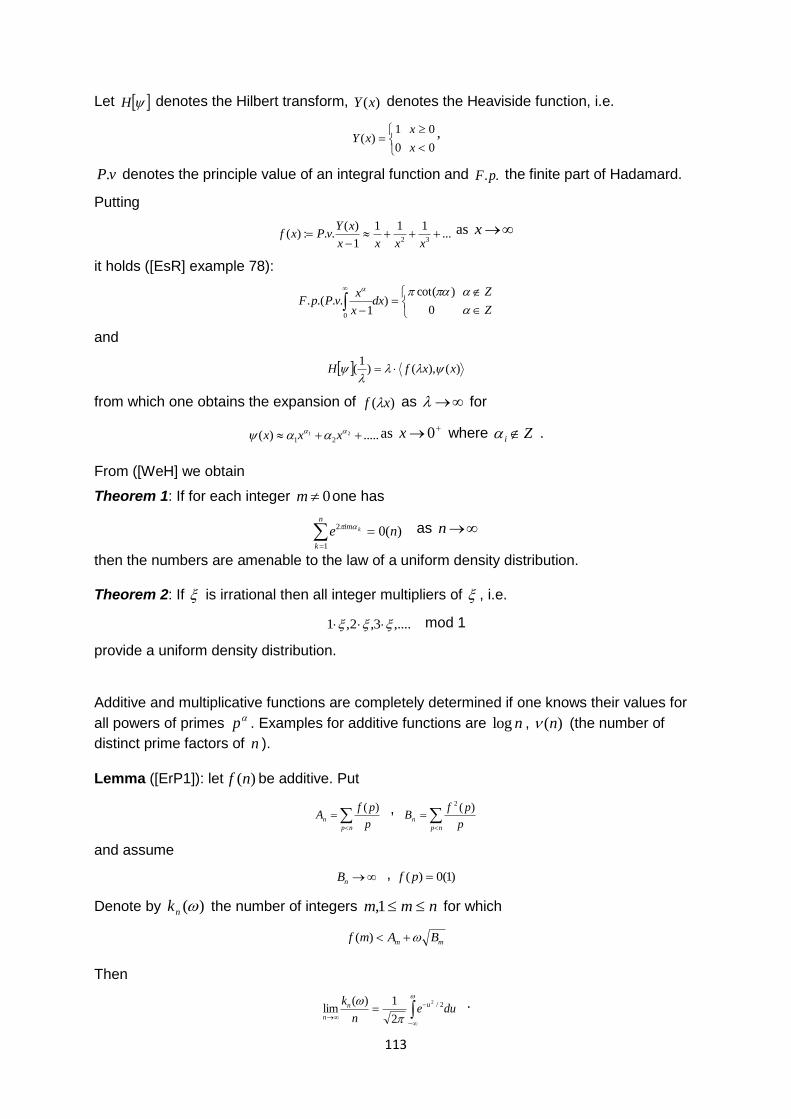
113
Let H denotes the Hilbert transform, )(xY denotes the Heaviside function, i.e.
0
0
0
1)(
x
xxY ,
vP. denotes the principle value of an integral function and ..pF the finite part of Hadamard.
Putting
...111
1
)(..:)(
32
xxxx
xYvPxf as x
it holds ([EsR] example 78):
Z
Zdx
x
xvPpF
0
)cot()
1...(.0
and
)(),()1
( xxfH
from which one obtains the expansion of )( xf as for
.....)( 21
21 xxx as
0x where Zi .
From ([WeH] we obtain
Theorem 1: If for each integer 0m one has
)(01
2ne
n
k
im k
as n
then the numbers are amenable to the law of a uniform density distribution.
Theorem 2: If is irrational then all integer multipliers of , i.e.
,....3,2,1 mod 1
provide a uniform density distribution.
Additive and multiplicative functions are completely determined if one knows their values for
all powers of primes p . Examples for additive functions are nlog , )(n (the number of
distinct prime factors of n ).
Lemma ([ErP1]): let )(nf be additive. Put
np
np
pfA
)( ,
np
np
pfB
)(2
and assume
nB , )1(0)( pf
Denote by )(nk the number of integers nmm 1, for which
mm BAmf )(
Then
duen
k un
n
2/2
2
1)(lim .
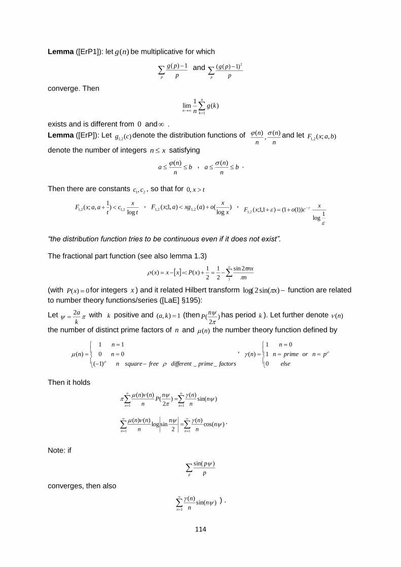
114
Lemma ([ErP1]): let )(ng be multiplicative for which
p p
pg 1)( and
p p
pg 2)1)((
converge. Then
n
kn
kgn 1
)(1
lim
exists and is different from 0 and .
Lemma ([ErP]): Let )(2,1 cg denote the distribution functions of n
n
n
n )(,
)( and let ),;(2,1 baxF
denote the number of integers xn satisfying
bn
na
)( , bn
na
)( .
Then there are constants
21, cc , so that for tx ,0
t
xc
taaxF
log)
1,;( 2,12,1 , )
log()(),1;( 2,12,1
x
xoaxgaxF ,
1log
))1(1()1,1;(2,1
xcoxF
“the distribution function tries to be continuous even if it does not exist”. The fractional part function (see also lemma 1.3)
1
2sin
2
1
2
1)(:)(
n
nxxPxxx
(with 0)( xP for integers x ) and it related Hilbert transform )sin(2log( x function are related
to number theory functions/series ([LaE] §195):
Let k
a2 with k positive and 1),( ka (then )
2(
nP has period k ). Let further denote )(n
the number of distinct prime factors of n and )(n the number theory function defined by
factorsprimedifferentfreesquaren
n
n
n
__
0
1
)1(
0
1
)(
, pnor
else
primen
n
n
0
0
1
1
)(
Then it holds
11
)sin()(
)2
()()(
nn
nn
nnP
n
nn
11
)cos()(
2sinlog
)()(
nn
nn
nn
n
nn
.
Note: if
p p
p )sin(
converges, then also
)sin()(
1
nn
n
n
) .
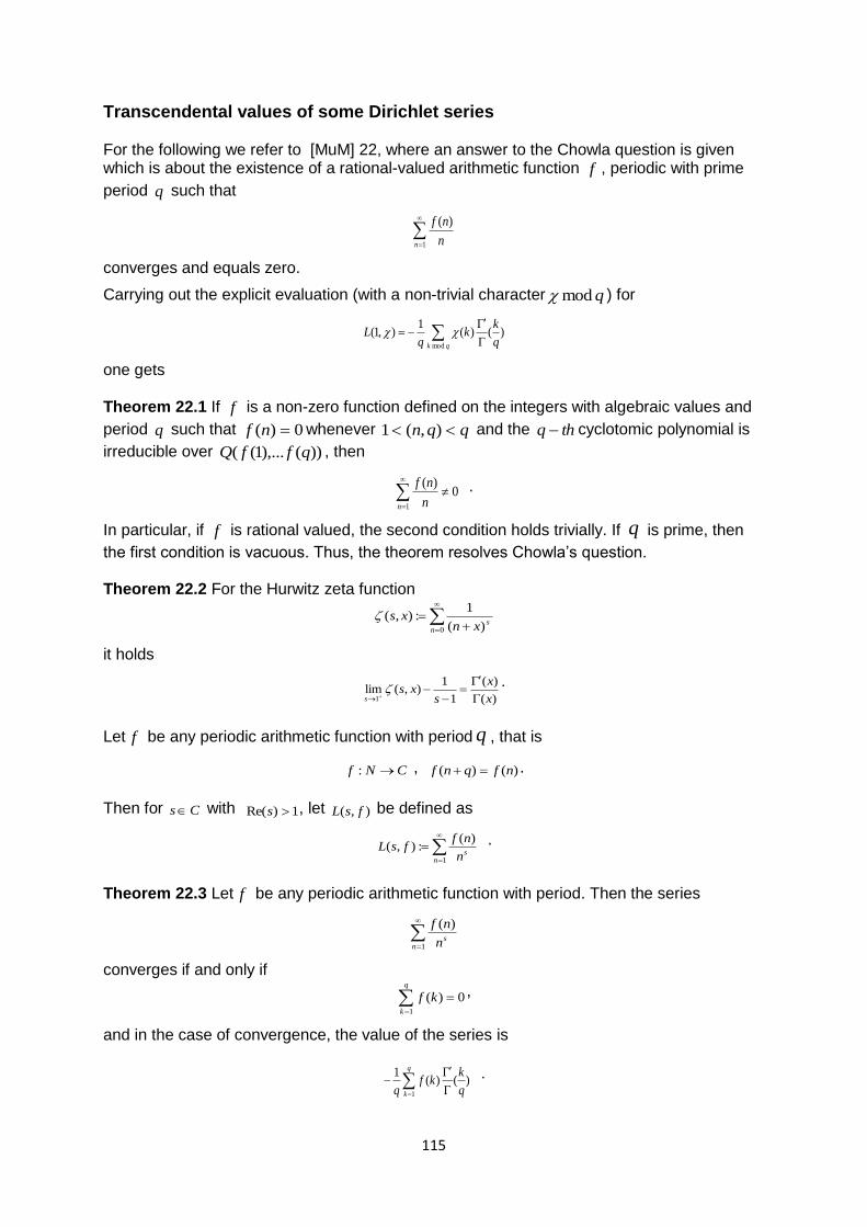
115
Transcendental values of some Dirichlet series For the following we refer to [MuM] 22, where an answer to the Chowla question is given which is about the existence of a rational-valued arithmetic function f , periodic with prime
period q such that
1
)(
n n
nf
converges and equals zero.
Carrying out the explicit evaluation (with a non-trivial character qmod ) for
)()(1
),1(mod q
kk
qL
qk
one gets Theorem 22.1 If f is a non-zero function defined on the integers with algebraic values and
period q such that 0)( nf whenever qqn ),(1 and the thq cyclotomic polynomial is
irreducible over ))(),...1(( qffQ , then
0)(
1
n n
nf .
In particular, if f is rational valued, the second condition holds trivially. If q is prime, then
the first condition is vacuous. Thus, the theorem resolves Chowla’s question. Theorem 22.2 For the Hurwitz zeta function
0 )(
1:),(
nsxn
xs
it holds
)(
)(
1
1),(lim
1 x
x
sxs
s
.
Let f be any periodic arithmetic function with period q , that is
CNf : , )()( nfqnf .
Then for Cs with 1)Re( s , let ),( fsL be defined as
1
)(:),(
nsn
nffsL .
Theorem 22.3 Let f be any periodic arithmetic function with period. Then the series
1
)(
nsn
nf
converges if and only if
q
k
kf1
0)( ,
and in the case of convergence, the value of the series is
)()(1
1 q
kkf
q
q
k
.
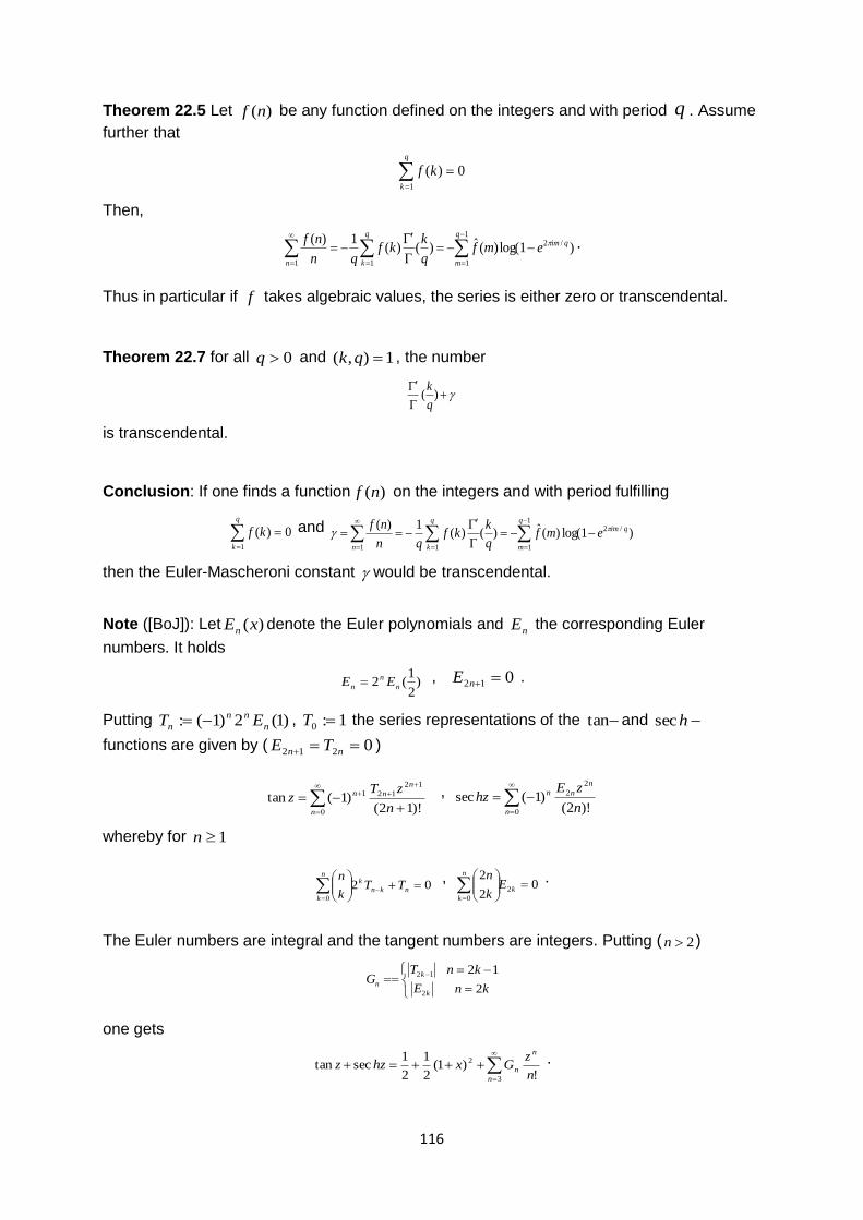
116
Theorem 22.5 Let )(nf be any function defined on the integers and with period q . Assume
further that
q
k
kf1
0)(
Then,
1
1
/2
11
)1log()(ˆ)()(1)(
q
m
qimq
kn
emfq
kkf
qn
nf .
Thus in particular if f takes algebraic values, the series is either zero or transcendental.
Theorem 22.7 for all 0q and 1),( qk , the number
)(
q
k
is transcendental. Conclusion: If one finds a function )(nf on the integers and with period fulfilling
q
k
kf1
0)( and
1
1
/2
11
)1log()(ˆ)()(1)( q
m
qimq
kn
emfq
kkf
qn
nf
then the Euler-Mascheroni constant would be transcendental.
Note ([BoJ]): Let )(xEn
denote the Euler polynomials and nE the corresponding Euler
numbers. It holds
)2
1(2 n
n
n EE , 012 nE .
Putting )1(2)1(: n
nn
n ET , 1:0 T the series representations of the tan and hsec
functions are given by ( 0212 nn TE )
0
12
121
)!12()1(tan
n
n
nn
n
zTz ,
0
2
2
)!2()1(sec
n
n
nn
n
zEhz
whereby for 1n
020
nkn
kn
k
TTk
n , 0
2
22
0
k
n
k
Ek
n .
The Euler numbers are integral and the tangent numbers are integers. Putting ( 2n )
kn
kn
E
TG
k
k
n2
12
2
12
one gets
3
2
!)1(
2
1
2
1sectan
n
n
nn
zGxhzz .
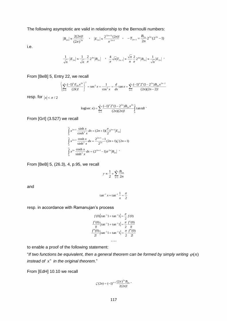
117
The following asymptotic are valid in relationship to the Bernoulli numbers:
nn
nB
22)2(
)!2(2
,
12
)1(2
2
)!2(2
n
n
n
nE
, )12(22
22212
nnnn
n
BT
i.e.
n
n
n Bn
En
2
4
2 2211
,
nn
n
n En
Bn
nTn 22
4
12
12
24
.
From [BeB] 5, Entry 22, we recall
1
22
2
2
2
2
2
0
2
2
)!22)(2(
)21(2)1(tan
cos
1sec
)!2(
)1(
n
n
n
nnn
k
k
k
k
nn
xBx
dx
d
xx
k
xE
resp. for 2/x
x
n
n
n
nnn
tdtnn
xBx
01
2
2
2
tan)!2)(2(
)21(2)1()log(sec .
From [GrI] (3.527) we recall
0
2
12
2
12 )2
)(12(cosh
sinhn
nn Endxx
xx
0
2
12
2
12 )12()12(2
12
sinh
coshnndx
x
xx
n
nn
0
2
212
2
2 )12(sinh
coshn
nnn Bdxx
xx
.
From [BeB] 5, (26.3), 4, p.95, we recall
1
2
22
1
n
n
n
B
and
2
1tantan 11
xx
resp. in accordance with Ramanujan’s process
)0(2
1tan1tan)0( 11 ff
!1
)0(
21tan1tan
!1
)0( 11 ff
!2
)0(
21tan1tan
!2
)0( 11 ff
….
to enable a proof of the following statement:
“If two functions be equivalent, then a general theorem can be formed by simply writing )(n
instead of nx in the original theorem.”
From [EdH] 10.10 we recall
)!2(2
)2()1()2( 2
21
n
Bn n
nn
.
118
References
[AbM] Abramowitz M., Stegen I. A., Handbook of Mathematical Functions, Dover Publications, Inc., New York, 1965 [AlA] Al-Fhaid A. S., Continued Fraction Evaluation of the Error Function, JKAU Sci, 18, 85-92, 2006 [AmT] Amdeberhan T., Coffey M., Espinosa O., Koutschan C., Manna D., Moll V., integrals of powers of log-gamma, Proc. Amer. Math. Soc., 139, 535-545, 2011
[AnJ] Annett J. F., Superconductivity, Superfluids and Condensates, Oxford University Press, Oxford, New York, 2003
[ApT] Apostol T. M., Introduction to Analytic Number Theory, Springer Verlag, 2000
[ArI] Aref’eva I. Y., Volovich I. V., Quantization of the Riemann Zeta-Function and Cosmology, Int. J. Geom. Methods Mod. Phys., 4:5 (2007), 881–895
[BaB] Bagchi B., On Nyman, Beurling and Baez-Duarte’s Hilbert space reformulation of the Riemann Hypothesis, Indian Statistical Institute, Bangalore Centre, (2005), www.isibang.ac.in [BaB1] Bagchi B., A Joint Universality Theorem for Dirichlet L-Functions, Math. Z. 181,319-334, 1982 [BeB] Berndt B. C., Andrews G. E., Ramanujan´s Notebooks Part I, Springer Verlag, New York, Berlin, Heidelberg, Tokyo, 1989 [BeB1] Berndt B. C., Andrews G. E., Ramanujan´s Notebooks Part II, Springer Verlag, New York, Berlin, Heidelberg, Tokyo, 1985 [BiP] Biane P., Pitman J., Yor M., Probability laws related to the Jacobi Theta and Riemann Zeta function, and Brownian excursions, Amer. Math. Soc., 38, No 4, 435-465, 2001
[BiI] BiswasI., Nag S., Jacobians of Riemann surfaces and the Sobolev space 2/1H on the circle, Math. Research Letters, 5, 281-292, 1998 [BiJ] Bittencourt J. A., Fundamentals of Plasma Physics, Springer Verlag, New York, Berlin, Heidelberg, Hong Kong, London, Milan, Paris, Tokyo, 2004 [BoJ] Borwein J. M., Borwein P. B., Dilcher K., Pi, Euler numbers, and Asymptotic Expansion, Amer. Math. Soc., Vol. 96, No. 8, 681-687, 1989 [BoJe] Bourgain J., Kozma G., One cannot hear the winding number, J. Eur. Math. Soc., 9, 637-658, 2007 [BrK] Braun K., Interior Error Estimates of the Ritz Method for Pseudo-Differential Equations, Jap. Journal of Applied Mathematics, 3, 1, 59-72, 1986 [BrK1] Braun K., Global existence and uniqueness of 3D Navier-Stokes equations, navier-stokes-equations@com [BrK2] Braun K., A Note to the Bagchi Formulation of the Nyman-RH-Criterion, www.riemann-hypothesis.de
119
[BrK3] Braun K., A new ground state energy model, www.quantum-gravitation.de [BrT] Bromwich T. J., An Introduction To The Theory Of Infinite Series, Merchant Books, 1908 [BuH] Buchholtz H., The confluent Hypergeometric Function: with Special Emphasis on its Applications, Springer Verlag, Berlin, Heidelberg, 1969 [BuD] Bump D., Choi K.-K., Kurlberg P., Vaaler J., A Local Riemann Hypothesis I , Math.
Zeit. 233 (2000) pp. 1-19
[BuP] Butzer P. L., Trebels W., Hilberttransformation, gebrochene Integration und
Differentiation, Springer Fachmedien Wiesbaden GmbH, 1967
[CaD] Cardon D. A., Convolution operators and zeros of entire functions, Proc. Amer. Math. Soc., 130, 6 (2002) 1725-1734 [CeC] Cercignani C., Theory and application of the Boltzmann equation, Scottish Academic Press, Edingburgh and London, 1975 [ChD] Chamorro D., Remarks on a fractional diffusion transport equation with applications to the critical dissipative quasi-geostrophic equation, arXiv:10073919 [ChF] Chen F. F., Introduction to plasma physics and controlled fusion, Plenum Press, New York, 1984 [CaT] Chihara T. S., An introduction to orthogonal polynomials, Mathematics and its Applications 13, Gordon and Breach, New York, 1978 [CoA] Cordoba A., Cordoba D., Fontelos M. A., Integral inequalities for the Hilbert transform applied to a nonlocal transport equation, J. Math. Pures Appl. 86, 529-540, 2006 [DeP] Degond P., Spectral Theory of the Linearized Vlasov-Poisson Equation, Trans. Americ. Math. Soc., 294, 2, 435-453, 1986 [DiD] Dickinson, D., On Lommel and Bessel Polynomials, Doctoral Dissertation submitted to University of Michigan, 1953 [DiG] Dirac G., Note on a problem in additive number theory, J. London M. S., 26, 312-313,
1951
[DuR] Duffin R. J., Weinberger H. F., Dualizing the Poisson summation formula, Proc. Natl. Acad. Sci. 88 (1991) pp. 7348-7350 [DuR1] Duffin R. J., Hilbert Transforms in Yukawan Potential Theory, Proc. Nat. Acad. Sci., 69, 12, 3677-3679, 1972 [EdH] Edwards H. M., Riemann´s Zeta Function, Dover Publications, Inc., Mineola, New York, 1974 [ErP] Erdös P., On the distribution of numbers of the form and on some related questions, Pacific J. Math., Vol. 52, 1, 59-65, 1974
120
[ErP1] Erdös P., On additive arithmetical functions and applications of probability to number theory, Pacific J. Math., Vol. 71, 2, 275-294, 1977 [EsR] Estrada R., Kanwal R. P., Asymptotic Analysis: A Distributional Approach, Birkhäuser, Boston, Basel, Berlin, 1994 [FaM] Farge M., Schneider K., Wavelets: application to turbulence, University Warnick, lectures, 2005 [FaM1] Farge M., Wavelet transforms and their applications to turbulence, Annu. Rev. Fluid Mech. 24, 395-457, 1992 [GaD] Gaier D., Konstruktive Methoden der konformalen Abbildung, Springer-Verlag, Berlin,
1964
[FeE] Fermi E., thermodynamics, Dover Publications, Inc., New York, 1956
[GaG] Gasper G., Using sums of squares to prove that certain entire functions have only real
zeros, Fourier Analysis, Analytic and Geometric Aspects, W.O. Bray, P.S. Milojevic and C.V.
Stanojevic, eds., Marcel Dekkar, 171-186, 1994
[GlR] Glassey R., Schaeffer J., Time decay for solutions tot he linearized Vlasov equation,
Transport Theory Statist. Phys. 23, 4, 411-453, 1994
[GlR1] Glassey R., Schaeffer J., On time decay rates in Landau damping, Comm. Partial
Differential Equations, 20, 3-4, 647-676, 1995
[GaW] Gautschi W., Waldvogel J., Computing the Hilbert Transform of the Generalized Laguerre and Hermit Weight Functions [GrI] Gradshteyn I. S., Ryzhik I. M., Table of Integrals Series and Products, Fourth Edition, Academic Press, New York, San Francisco, London, 1965 [GrF] Grant F. C., Feix M. R., Fourier-Hermite solutions of the Vlasov equations in the linearized limit, Phys. Fluids, 10, 696-702, 1967 [GrT] Gronwall T. H., Some Asymptotic Expressions in the Theory of Numbers, Trans. Americ. Math. Soc., 14, No 1, 113-122, 1913 [HaG] Hardy G. H., Riesz M., The general theory of Dirichlet’s series, Cambridge University Press, Cambridge, 1915 [HaG1] Hardy G. H., Notes on special systems of orthogonal functions (II): On functions orthogonal with respect to their own zeros, J. Lond. Math. Soc. 14 (1939), 37-44 [HaG2] Hardy G. H., Littlewood J. E., Some problems of “Partitio Numerorum”; III, On the expression of a number as a sum of primes, Acta. Math., 44 (1923) 1-70
[HaH] Hamburger H., Über einige Beziehungen, die mit der Funktionalgleichung der Riemannschen Zeta-Funktion äquivalent sind, Math. Ann. 85 (1922) pp. 129-140 [HeH] Hedenmalm H., Dirichlet series and Functional Analysis, Royal Institute of Technology, Stockholm
121
[HeH] Helfgott H. A., Minor Arcs for Goldbach’s Problem, Major Arcs for Goldbach’s Problem, arXiv.org
[IvA] Ivic A., The Riemann Zeta-Function, Theory and Applications, Dover Publications Inc., Mineola, New York, 2003 [JoS] Joffily S., Jost function, prime number and Riemann zeta function, Rio devJaneiro, CBPF, Centro Brasileiro de Pesquisas Fisicas, 2003 [JoS1] Joffily S., The Riemann Zeta Function and Vacuum Spectrum, arXiv.org, 2004 [KaM] Kac M., Probability methods in some problems of analysis and number theory, Bull. Am. Math. Soc., 55, 641-655, (1949) [KaY] Kato Y., The coerciveness for integro-differential quadratic forms and Korn’s inequality, Nagoya Math. J. 73, 7-28, 1979 [KoA] Kolmogoroff A., Une contribution à l’étude de la convergence des séries de Fourier, Fund. Math. Vol. 5, 484-489 [KoJ] Korevaar J., Distributional Wiener-Ikehara theorem and twin primes, Indag. Mathem. N. S., 16, 37-49, 2005 [KoV] Kowalenko V., Frankel N.E., Asymptotics for the Kummer Function of Bose Plasmas, J. Math. Phys. 35, 6179, 1994 [KoW] Koppelmann W., Pincus J. D., Spectral Representations for Finite Hilbert Transformations, Math. Zeitschr. 71, 399-407, 1959 [LaG] Lachaud G., Spectral analysis and the Riemann hypothesis, J. Comp. Appl. Math., 160, 175-190, 2003 [LaE] Landau E., Die Lehre von der Verteilung der Primzahlen I, II, Teubner Verlag, Leipzig, Berlin, 1909 [LaE1] Landau E., Ueber die zahlentheoretische Function )(n und ihre Beziehung zum
Goldbachschen Satz, Nachrichten von der Gesellschaft der Wissenschaften zu Göttingen, Mathematische-Physikalische Klasse, Vol. 1900, p. 177-186, 1900 [LeN] Lebedev N. N., Special Functions and their Applications, translated by R. A. Silverman, Prentice-Hall, Inc., Englewood Cliffs, N. Y., 1965 [LiI] Lifanov I., K., Nenashev A. S., Generalized functions on Hilbert spaces, singular integral equations, and problems of aerodynamics and electrodynamics, Differential Equations, 43, 6, 862-872, 2007 [LiF] Lima F. S., On the possible exceptions for the transcendence of the log-gamma function at rational entries, arXiv.math, arXiv:0908.3253 [LiJ] Linnik Ju., V., The Dispersion Method in Binary additive Problems, American Mathematical society Providence, Rhode Island, 1963 [LiP] Lions P. L., Compactness in Boltzmann’s equation via Fourier integral operators and applications, J. Math. Kyoto Univ. 34, 2, 391-427, 1994
122
[LiP1] Lions P. L., On Boltzmann and Landau equations, Phil. Trans. R. Soc. Lond. A, 346, 191-204, 1994 [LuB] Lucke B., Zur Hardy-Littlewoodschen Behandlung des Goldbachschen Problems, Inaugural-Dissertation, Georg August-University Göttingen, 1926 [MaJ] Mashreghi J., Hilbert Transform of flog , Proc. Amer. Math. Soc., 130, No 3, 683-688,
2001 [McJ] McCabe J. H., A Continued Fraction Expansion, with a Truncation Error Estimate, for Dawson’s Integral, Math. Comp, Vol. 20, No. 127, (1974) p. 811-816 [McC] McMullen C. , Complex Analysis, Course Notes, Harward University Fall 2000, 2006, 2010 [MoC] Mouhot C., Villani C., On Landau Damping, AMS Subject Classification. 82C99 (85A05, 82D10) [MuM] Murty M. R., Rath P., Transcendental Numbers, Springer New York, Heidelberg, Dordrecht, London, 2013 [NaS] Nag S., Sullivan D., Teichmüller theory and the universal period mapping via quantum calculus and the H space on the circle, Osaka J. Math., 32, 1-34, 1995 [NaC] Nasim C., On the summation formula of Voronoi, Trans. Americ. Math. Soc., 163, (1972) [NiN] Nilsen N., Handbuch der Theorie der Gammafunktion, Chelsea Publishing Company, Bronx, New York, 1965 [OlJ] Olden J.-F., Local Properties of Hilbert spaces of Dirichlet series, Journal of Functional analysis, 261, 2669-2696, 2011 [OlF] Olver F. W. J., Asymptotics and Special Functions, Academic Press, Inc., Boston, San Diego, New York, London, Sydney, Tokyo, Toronto, 1974 [OsH] Bd. 1, Ostmann H., Additive Zahlentheorie, Springer-Verlag, Berlin, Heidelberg, New-York, 1969 [OsH] Bd. 2, Ostmann H., Additive Zahlentheorie, Springer-Verlag, Berlin, Heidelberg, New-York, 1969 [PaJ] Parker J. T., Dellar P. J., Fourier-Hermite spectral representation for the Vlasov-Poisson system in the weakly collisional limit, Journal of Plasma Physics, 81, 2, 2015 [PeR] Peralta-Fabi R., An integral representation oft he Navier-Stokes equations-I, Revista Mexicana de Fisica 31, 1, 57-67, 1984 [PeO] Perron O., Die Lehre von den Kettenbrüchen, Analytisch-funktionentheoretische Kettenbrüche, B. G. Teubner Verlag, Stuttgart, 1957 [PeB] Petersen B. E., Introduction to the Fourier Transform & Pseudo-Differential Operators, Pitman Publishing Limited, Boston, London, Melbourne
123
[PoG] Polya G., Über die algebraisch-funktionentheoretischen Untersuchungen von J. L. W. V. Jensen, Mathematisk-fysiske Meddelelsev VII 17 (1927), 1-33 [PoG1] Polya G., Bemerkungen über die Integraldarstellung der Riemannschen Zeta-Funktion, Acta Mathematica 48, 305-317 (1926) [PoG2] Polya G., Über trigonometrische Integrale mit nur reellen Nullstellen, J. rein. und angew. Math. 158 (1927) pp. 6-18 [PoG3] Polya G., Über die Nullstellen gewisser ganzer Funktionen, Math. Zeit. 2 (1918), 352-383, also, Collected Papers, Vol II, 166-197 [PrK] Prachar K., Primzahlverteilung, Springer-Verlage, Berlin, Göttingen, Heidelberg, 1957 [RaH] Rademacher H., Topics in Analytic Number Theory, Springer-Verlag, Berlin, Heidelberg, New York, 1973 [ScL] Schnirelmann L., Über additive Eigenschaften von Zahlen, Math. Ann. 107, 646-690, 1933 [ScW] Schwarz W., Einführung in Methoden und Ergebnisse der Primzahltheorie, BI,Mannheim, Zürich, 1969
[SeA] Sedletskii A. M., Asymptotics of the Zeros of Degenerate Hypergeometric Functions, Mathematical Notes, Vol. 82, No. 2 (2007) 229-237
[SeA1] Sedletskii A. M., „On the Zeros of Laplace Transforms“, Mathematical Notes, Vol. 76, No. 6 (2004) 883-892
[ShE] Shamir E., Reduced Hilbert transforms and singular integral equations, J. d’Analyse Math. 12, 227-305, 1964
[ShA] Shidlovskii A. B., Transcendental Numbers,Walter de Gruyter, Berlin, New York, 1989
[StE] Stein E., M., Harmonic Analysis, Princeton University Press, Princeton, New Jersay, 1993
[SzG] Szegö G., Orthogonal Polynomials, American Mathematical Society, Providence, Rhode Island, 2003
[TiE] Titchmarsh E. C., The Theory of the Riemann Zeta-function, Oxford University Press
Inc., New York, first published 1951, Second Edition 1986
[ViI] Vinogradov, I. M., Representation of an odd number as the sum of three primes, Dokl. Akad. Nauk SSSR 15, 291-294 (1937) [ViJ] Vindas J., Estrada R., A quick distributional way to the prime number theorem, Indag. Mathem., N.S. 20 (1) (2009) 159-165 [VlV] Vladimirow V. S., Drozzinov Y. N., Zavialov B. I., Tauberian Theorems for Generalized Functions, Kluwer Academic Publisher, Dordrecht, Boston, London, 1988 [VoA] Voros A., A sharpening of Li’s criterion for the Riemann Hypothesis, Math. Phys. Anal. and Geometry, 9, 1, 53-63, 2006
124
[WaA] Walfisz A., Weylsche Exponentialsummen in der neueren Zahlentheorie, VEB Deutscher Verlag der Wissenschaften, Berlin, 1963 [WaG] Watson G. N., A Treatise on the Theory of Bessel Functions, Cambridge University Press, Cambridge, 2nd edition first published 1944, reprinted 1996, 2003, 2004, 2006 [WeH] Weyl H., Über die Gleichverteilung von Zahlen mod. Eins, Math. Annalen, 77, 313-352, 1916 [WhE] Whittaker E. T., Watson G. N., A Course of Modern Analysis, Cambridge University Press, Cambridge, 1902 [WhJ] Whittaker J. M., Interpolatory Function Theory, Cambridge University Press, 1935 [ZyA] Zygmund A., Trigonometric series, Cambridge University Press, Cambridge, 1959 [ZyA1] Zygmund A., On the convergence of lacunary trigonometric series, Fund. Math. Vol. 16, 90-107, 1939