A LANGUAGE AND ENVIRONMENT FOR ANALYSIS OF DYNAMICS …wai/Papers/IJAIT07leadsto.pdf · A Language and Environment for Analysis of Dynamics by SimulaTiOn 5 Fig. 2. Example of a graphical

International Journal on Artificial Intelligence Tools Vol. XX, No. X (2006) 1–43 World Scientific Publishing Company

1

A LANGUAGE AND ENVIRONMENT FOR ANALYSIS OF DYNAMICS BY SIMULATION

Tibor Bosse

Vrije Universiteit Amsterdam, Department of Artificial Intelligence, De Boelelaan 1081a, 1081 HV Amsterdam, The Netherlands

[email protected]

Catholijn M. Jonker

Radboud Universiteit Nijmegen, Nijmegen Institute for Cognition and Information, Montessorilaan 3, 6525 HR Nijmegen, The Netherlands

[email protected]

Lourens van der Meij


[email protected]

Jan Treur


[email protected]

This article presents the language and software environment LEADSTO that has been developed to model and simulate dynamic processes in terms of both qualitative and quantitative concepts. The LEADSTO language is a declarative order-sorted temporal language, extended with quantitative notions like integer and real. Dynamic processes can be modelled in LEADSTO by specifying the direct temporal dependencies between state properties in successive states. Based on the LEADSTO language, a software environment was developed that performs simulations of LEADSTO specifications, generates data-files containing traces of simulation for further analysis, and constructs visual representations of traces. The approach proved its worth in a number of research projects in different domains.

Keywords: Simulation; causal relations.

1. Introduction

In simulations, various formats are used to specify the basic mechanisms or causal relations within a process1, 2, 3, 4, 5, 6, 7, 8, 9. Depending on the domain of application, such basic mechanisms need to be formulated quantitatively or qualitatively. Usually, within a given application, explicit (temporal) boundaries can be given in which the mechanisms take effect. This is the case, for example, in the following statement: “ from the time of planting of an avocado pit, it takes 4 to 6 weeks for a shoot to appear” . Another example is: “with a lower threshold of 5˚C, alfalfa takes 555 to 890 growing degree-days to

Tibor Bosse, Catholijn M. Jonker, Lourens van der Meij, and Jan Treur 2

bloom”. Here, a growing degree-day is a day in which the mean daily temperature is one degree above the base temperature of that particular crop. Yet another example, in the domain of psychology, is the following statement: “The reaction time of a healthy adolescent lies between 180 and 220 ms” .

In all of the above examples, in order to simulate the process that takes place, it is important to model its dynamics. When considering current approaches to modelling dynamics, the following two classes can be identified: logic-oriented modelling approaches, and mathematical modelling approaches, usually based on difference or differential equations. Logic-oriented approaches are good for expressing qualitative relations, but less suitable for working with quantitative relationships. Mathematical modelling approaches (e.g., Dynamical Systems Theory3, 8, 9), are good for the quantitative relations, but expressing conceptual, qualitative relationships with them is hard to impossible. In this article, the Language and Environment for Analysis of Dynamics by SimulaTiOn (LEADSTO) is proposed as a language that combines the possibilities of expressing qualitative and quantitative relations.

In Section 2, a formal definition of the LEADSTO language (in terms of both structure and semantics) is given, and it is shown how the language can be used to model dynamics. Section 3 provides examples of existing case studies in which LEADSTO has been applied. Section 4 describes the tools that support the LEADSTO modelling environment in detail. In particular, the LEADSTO Property Editor and the LEADSTO Simulation Tool are discussed. Section 5 compares the approach to related modelling approaches, and Section 6 is a conclusion.

2. The LEADSTO Language

Dynamics can be modelled in different forms. For example, the Dynamical Systems Theory (DST3, 8, 9), which is based on the area within Mathematics called calculus, advocates to model dynamics by continuous state variables and changes of their values over (continuous) time. In particular, systems of differential or difference equations are used for this type of modelling. This may work well in applications where the world states can be modelled (in a quantitative manner) by real-valued state variables, and where the world’s dynamics shows continuous changes in these world states, which can be modelled by mathematical relationships between real-valued variables.

However, not for all applications dynamics can be modelled in a quantitative manner as required for DST. Sometimes qualitative changes form an essential aspect of the dynamics of a process. For example, to model the dynamics of reasoning processes, usually a quantitative approach will not work. In such processes, states are characterised by qualitative state properties, and changes by transitions between such state properties. For such applications, often qualitative, discrete modelling approaches are advocated, such as variants of modal temporal logic10. However, using such non-quantitative methods, the more precise timing relations are lost too.

A Language and Environment for Analysis of Dynamics by SimulaTiOn

3

2.1. Structure of the LEADSTO Language

The LEADSTO language enables one to model direct temporal dependencies between two state properties in successive states, also called dynamic properties. A specification of dynamic properties in LEADSTO format has as advantages that it is executable and that it can often easily be depicted graphically. For the approach described in this paper, the choice has been made to consider time as continuous, described by real values, but for state properties, both quantitative and qualitative variants can be used. The approach subsumes approaches based on simulation of differential or difference equations, and discrete qualitative modelling approaches, but also combines them. For example, it is possible to model the exact (real-valued) time interval for which some qualitative property holds. Moreover, the relationships between states over time are described by either logical or mathematical means, or a combination thereof. This will be explained below in more detail.

Dynamics is considered as evolution of states over time. The notion of state as used here is characterised on the basis of an ontology defining a set of properties that do or do not hold at a certain point in time. Ontologies are specified as signatures in order-sorted predicate logic, i.e., sets of sorts and subsort relations, constants in sorts, functions and predicates over sorts11.

Definition (State Properties) Let Ont be a given ontology Ont. a) The set of state atoms (or atomic state properties) based on Ont is denoted by

APROP(Ont), and the set of state ground atoms by GAPROP(Ont).

b) The set of state properties STATPROP(Ont) based on Ont consists of the propositions that can be made (using conjunction, negation, disjunction, implication) from the atoms. Moreover, GSTATPROP(Ont) is the subset of ground state properties, based on ground atoms. A subset of the set of state properties is the set CONLIT(Ont) of conjunctions of literals (atoms or negations of atoms).

The textual LEADSTO format is defined as follows. Definition (LEADSTO format) Let a state ontology Ont be given. a) Any expression for Ont of the form

∀x1, ..., xn α →→e, f, g, h β where α (the antecedent) and β (the consequent) are state properties in CONLIT(Ont), with variables among x1, .., xn, and e, f, g, h non-negative real numbers, is a LEADSTO expression. When no variables nor quantifiers occur in this expression, it is called a LEADSTO ground expression. b) Any expression

holds_during_interval(α, t1, t2)


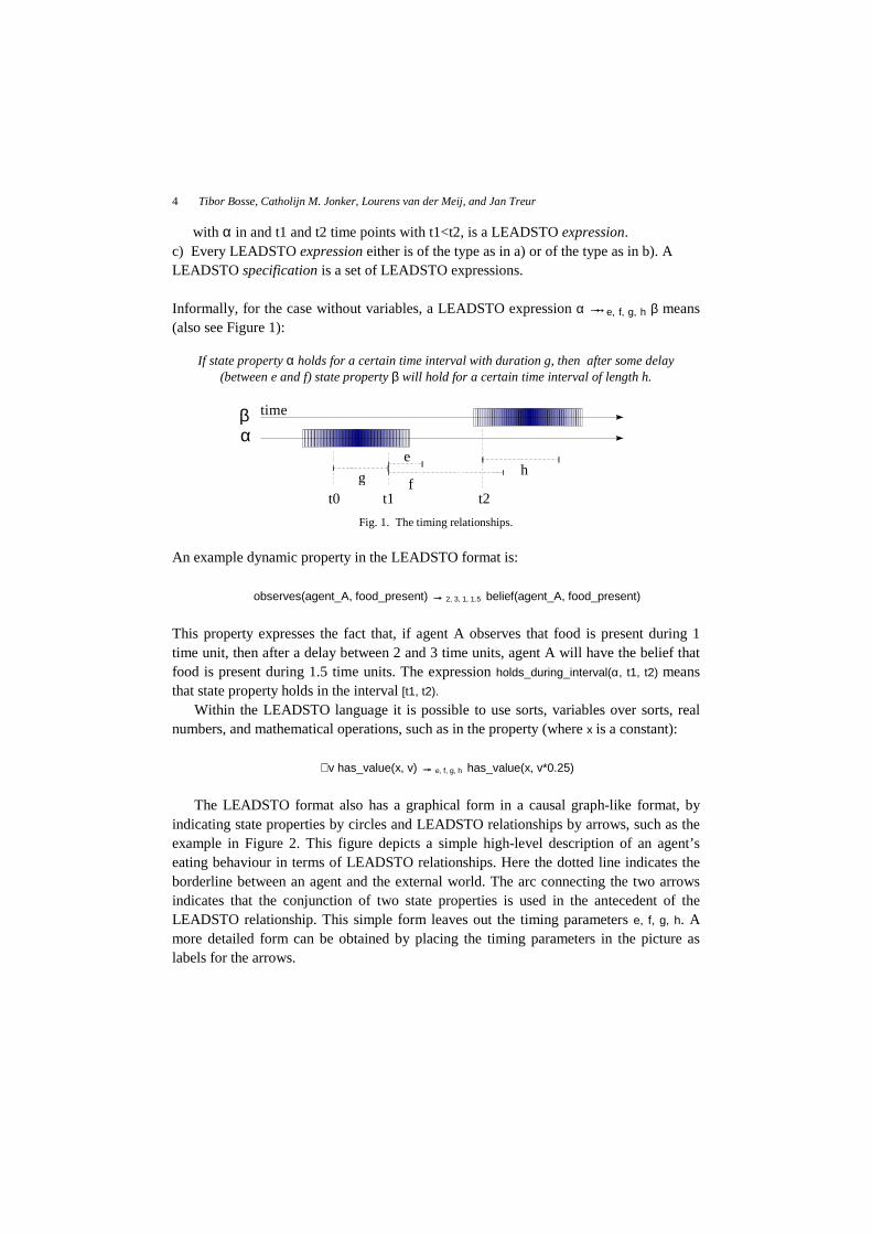
with α in and t1 and t2 time points with t1<t2, is a LEADSTO expression. c) Every LEADSTO expression either is of the type as in a) or of the type as in b). A LEADSTO specification is a set of LEADSTO expressions. Informally, for the case without variables, a LEADSTO expression α →→e, f, g, h β means (also see Figure 1):

If state property α holds for a certain time interval with duration g, then after some delay (between e and f) state property β will hold for a certain time interval of length h.

αβ

t1

e

g h

t2

time

ft0

Fig. 1. The timing relationships.

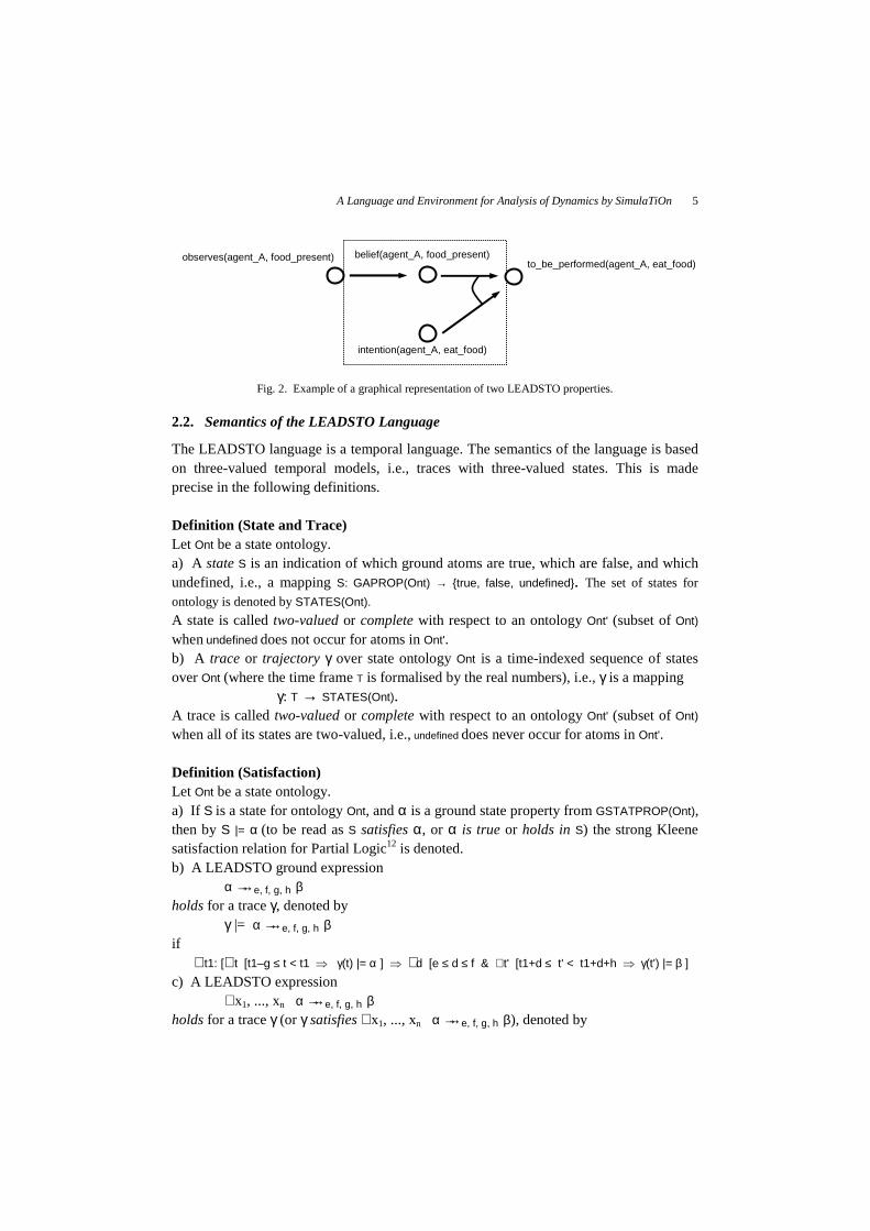
An example dynamic property in the LEADSTO format is:

observes(agent_A, food_present) →→ 2, 3, 1, 1.5 belief(agent_A, food_present)

This property expresses the fact that, if agent A observes that food is present during 1 time unit, then after a delay between 2 and 3 time units, agent A will have the belief that food is present during 1.5 time units. The expression holds_during_interval(α, t1, t2) means that state property holds in the interval [t1, t2).

Within the LEADSTO language it is possible to use sorts, variables over sorts, real numbers, and mathematical operations, such as in the property (where x is a constant):

∀v has_value(x, v) →→ e, f, g, h has_value(x, v*0.25)

The LEADSTO format also has a graphical form in a causal graph-like format, by

indicating state properties by circles and LEADSTO relationships by arrows, such as the example in Figure 2. This figure depicts a simple high-level description of an agent’s eating behaviour in terms of LEADSTO relationships. Here the dotted line indicates the borderline between an agent and the external world. The arc connecting the two arrows indicates that the conjunction of two state properties is used in the antecedent of the LEADSTO relationship. This simple form leaves out the timing parameters e, f, g, h. A more detailed form can be obtained by placing the timing parameters in the picture as labels for the arrows.


5

Fig. 2. Example of a graphical representation of two LEADSTO properties.

2.2. Semantics of the LEADSTO Language

The LEADSTO language is a temporal language. The semantics of the language is based on three-valued temporal models, i.e., traces with three-valued states. This is made precise in the following definitions. Definition (State and Trace) Let Ont be a state ontology. a) A state S is an indication of which ground atoms are true, which are false, and which undefined, i.e., a mapping S: GAPROP(Ont) → {true, false, undefined}. The set of states for

ontology is denoted by STATES(Ont).

A state is called two-valued or complete with respect to an ontology Ont' (subset of Ont)

when undefined does not occur for atoms in Ont'. b) A trace or trajectory γ over state ontology Ont is a time-indexed sequence of states over Ont (where the time frame T is formalised by the real numbers), i.e., γ is a mapping

γ: T → STATES(Ont). A trace is called two-valued or complete with respect to an ontology Ont' (subset of Ont)

when all of its states are two-valued, i.e., undefined does never occur for atoms in Ont'. Definition (Satisfaction) Let Ont be a state ontology. a) If S is a state for ontology Ont, and α is a ground state property from GSTATPROP(Ont), then by S |= α (to be read as S satisfies α, or α is true or holds in S) the strong Kleene satisfaction relation for Partial Logic12 is denoted. b) A LEADSTO ground expression

α →→e, f, g, h β holds for a trace γ, denoted by

γ |= α →→e, f, g, h β if

∀t1: [∀t [t1–g ≤ t < t1 � γ(t) |= α ] � ∃d [e ≤ d ≤ f & ∀t' [t1+d ≤ t' < t1+d+h � γ(t') |= β ]

c) A LEADSTO expression ∀x1, ..., xn α →→e, f, g, h β

holds for a trace γ (or γ satisfies ∀x1, ..., xn α →→e, f, g, h β), denoted by

intention(agent_A, eat_food)

belief(agent_A, food_present) to_be_performed(agent_A, eat_food)

observes(agent_A, food_present)


γ |= ∀x1, ..., xn α →→e, f, g, h β if all ground instances of α →→e, f, g, h β hold for γ. d) A LEADSTO expression holds_during_interval(α, t1, t2) holds for a trace γ, denoted by γ |= holds_during_interval(α, t1, t2) if

∀t [ t1 ≤ t < t2 � γ(t) |= α ] e) A trace γ satisfies a LEADSTO specification if it satisfies all expressions in this specification.

The state formulae α, β occurring in LEADSTO ground expressions have a relatively

simple structure. Strong Kleene semantics for them is defined by (where α, α1, …, αn are ground atoms):

S |= α1 ∧ .... ∧ αn ⇔ S |= α1 ∧ .... ∧ S |= αn S |= ¬ α ⇔ S(α) = false

S |= α ⇔ S(α) = true

2.3. The Use of LEADSTO Specifications for Simulation

An important use of the LEADSTO language is as a specification language for simulation models. As indicated above, on the one hand LEADSTO expressions can be considered as logical expressions with a declarative, temporal semantics, showing what it means that they hold in a given trace. On the other hand they can be used to specify basic mechanisms of a process and to generate (in general three-valued) traces that satisfy the formulae, similar to Executable Temporal Logic1, 13, 4, 5, 6, 7, 14, 15, 16, 17. A temporal formula in executable format is one according to the pattern past and current implies future Here the time frame is assumed to be discrete. A simple example of an executable temporal formula is (with C the current operator and X the next operator)

Ca ∧ Cb → Xc which states that always if in a state the state properties a and b hold, then in the next state property c holds. Simulation based on such a temporal formula can be performed by executing it in the following inductive sense:

1. Check the antecedents on the last generated state of the simulation trace

If a trace has been generated up to time point t, determine whether the conditions a and b hold in the state at t.

2. Collect the consequents for those antecedents that hold at the last generated state Examining in an exhaustive manner all temporal formulae in executable format defining a specification, a number of properties for the state at time t + 1 are determined; e.g., if a and b hold, then for the state at the next time point t + 1 the property c is to hold.

3. Build the next state by derived state properties


7

All collected consequents together provide a (partial) description of the next state at time t + 1.

4. Complete the next state By some form of completion (e.g., by a closed world assumption, making state properties false that are not derivable in a positive manner), this description can be made complete, obtaining the complete next state of the trace for t + 1.

Note that in steps 2. and 3. it is assumed that no contradictory consequents are derived. The modeller has the responsibility to ensure this. An advantage of this paradigm of Executable Temporal Logic is that simulation models are specified not in an algorithmic manner, but in a declarative logical manner. The relation between the specification and the constructed trace is that the trace is a model (in the logical sense) of the theory defined by the specification, i.e., all temporal formulae of the specification hold in the trace. A disadvantage of the discrete time frame assumption is that it does not allow specification of simulation models where variable real-valued time periods between the transitions play a role; however in LEADSTO this is possible. The procedure used for simulation of a LEADSTO specification is a variation on the procedure for Executable Temporal Logic shown above. For example, for step 1 not the last generated state is taken, but the past time interval is considered. Moreover, in step 3 and 4. the state properties are fixed for certain future time intervals instead of one state.

Not every trace satisfying the LEADSTO specification is generated in this way. First, generated traces satisfy the finite variability property, which expresses, informally stated, that between any two time points t0, t1 only a finite number of state changes occurs, or, equivalently, for the interval from t0 to t1 there is a minimal duration δ, such that between states always persist with duration at least δ. This is defined by:

Definition (Finite Variability) A trace γ has finite variability if ∀t0, t1>t0 ∃δ>0 [ ∀t [ t0 ≤ t & t ≤ t1 ] � ∃t2 [t2 ≤t & t<t2+δ & ∀t3 [ t2 ≤ t3 & t3 ≤ t2+δ ] ] � γ(t3) = γ(t) ] Second, another element that can play a role in the execution of a LEADSTO specification as a simulation model is the notion of trace completion, or temporal completion, based on a Closed World Assumption. This is based on the following concept: Definition (State Completion) Let Ont, Ont’ be state ontologies with Ont’ a subset of Ont and S a state for Ont. The completion of state S with respect to Ont' is the state c(S, Ont') defined by

c(S, Ont')(α) = true if S(α) = true c(S, Ont')(α) = false if S(α) = false

c(S, Ont')(α) = false if α is in Ont' and S(α) = undefined for all ground atoms α for Ont.


State completion can be applied (as an option) during execution of a LEADSTO specification, for parts of the state ontology, whenever for certain atoms in a state no truth values true or false are entailed by the specification on the basis of the previous states. In such a case it is possible to generate traces that are complete (two-valued) with respect to certain atoms, and satisfy the expressions in the specification. Note that this is not the same as taking a three-valued trace, and completing parts of its states: in this case it would be possible that certain LEADSTO expressions are no longer satisfied (for example, because some antecedent would become satisfied but not the consequent).

3. Applications

The LEADSTO environment has been used in a number of research projects in different domains. In this section, some of these projects will be summarised, with special attention for the role of LEADSTO in them. In general, these research projects can be divided into two categories: those focussing on single-agent dynamics (cognitive modelling), and those focussing on multi-agent dynamics (social modelling).

Examples of single-agent (or cognitive) processes that have been modelled using LEADSTO are human reasoning processes, eating regulation processes, and conditioning processes. Examples in multi-agent (or social) domains are ant colonies, organisations (e.g., a factory), and component-based software systems. In general, the research goal in these kinds of projects was to analyse the process under investigation by creating a detailed model of its dynamics. LEADSTO was used to formalise the basic mechanisms of these processes at a high level of abstraction. Since the LEADSTO format is executable, such mechanisms can be and have been used to generate simulation traces without additional programming.

Below, for three different domains, its formalisation in terms of dynamic properties and the resulting simulation model will be discussed. Section 3.1 describes a model of an adaptive dynamical system for eating regulation disorders18. Section 3.2 describes a model of human trace conditioning19. Section 3.3 describes the dynamics of an ant colony20. Thus, the first two examples address single-agent processes; the third example addresses a multi-agent process.

3.1. Eating Regulation Processes

The psychologist Martine Delfos created an adaptive dynamical model that describes normal functioning of eating regulation under varying metabolism levels. In one of her books21, Delfos uses this model as a basis for classification of eating regulation disorders, and of diagnosis and treatment within a therapy. Reasoning about the dynamic properties of this model (and disturbances of them) is performed in an intuitive, conceptual, but informal manner. In previous work18, this model was formalised in LEADSTO, and some simulations have been generated, both for wellfunctioning situations and for different types of malfunctioning situations that correspond to the first phase of well-known disorders such as anorexia (nervosa), obesitas, and bulimia. The local properties used for the formalisation are shown in Appendix A. Some examples are shown below:


9

LP6 (Weight through balance of amount eaten and energy used) Local property LP6 expresses a simple mechanism of how weight is affected by the day balance of amount eaten and energy used. Here γ is a fraction that specifies how energy affects the weight in kilograms. Formalisation: ∀E1,E2,W:REAL day_amount_eaten(E1) and day_used_energy(E2) and weight(W) →→0,0,1,25 weight(W + γ * (E1 – E2))

LP7 (Adaptation of amount to be eaten) Local property LP7 expresses a simple (logistic) mechanism for the adaptation of the eat norm based on the day amount of energy used. The eat norm indicates the amount of food that should be eaten in order to compensate for the amount of energy used on a particular day. Note that a fictive unit measure is used here, but this could easily be replaced by a more realistic measure (e.g., kilocalories). Moreover, α is the adaptation speed, β is the fraction of E that is the limit of the adaptation; normally β = 1. Formalisation: ∀E,N:REAL day_used_energy(E) and eat_norm(N) and time(24) →→0,0,1,25 eat_norm(N + α * N * (1 - N/βE))

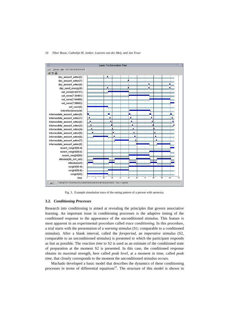
In the above example, the time units represent hours. Thus, dynamic property LP6 states, for example, that “if the antecedent holds for 1 hour, then the consequent will hold for 25 hours, with a delay of 0 hours”. Note that these dynamics properties combine real-valued, quantitative concepts with conceptual, qualitative concepts. In Figure 3 an example of a resulting simulation trace is shown. Here, time is on the horizontal axis; the state properties are on the vertical axis. A dark box on top of the line indicates that the property is true during that time period, and a lighter box below the line indicates that the property is false. For example, the state property eat_norm(6) is true from time point 0 to 25. This example illustrates the pattern of a person with anorexia. As the figure shows, the person has an eat norm (of 6 units) that is too low for the amount of energy used (of 8 units) per day. After a while, the eat norm converges a little bit to the amount of energy used, but this adaptation is not enough. The picture clearly demonstrates the consequences: the subject continuously eats an amount of food that is too low, compared to what she needs. Therefore, weight drops from 60 kilograms to 59.6 to 59.4, and this decreasing trend continues.


Fig. 3. Example simulation trace of the eating pattern of a person with anorexia.

3.2. Conditioning Processes

Research into conditioning is aimed at revealing the principles that govern associative learning. An important issue in conditioning processes is the adaptive timing of the conditioned response to the appearance of the unconditioned stimulus. This feature is most apparent in an experimental procedure called trace conditioning. In this procedure, a trial starts with the presentation of a warning stimulus (S1; comparable to a conditioned stimulus). After a blank interval, called the foreperiod, an imperative stimulus (S2, comparable to an unconditioned stimulus) is presented to which the participant responds as fast as possible. The reaction time to S2 is used as an estimate of the conditioned state of preparation at the moment S2 is presented. In this case, the conditioned response obtains its maximal strength, here called peak level, at a moment in time, called peak time, that closely corresponds to the moment the unconditioned stimulus occurs.

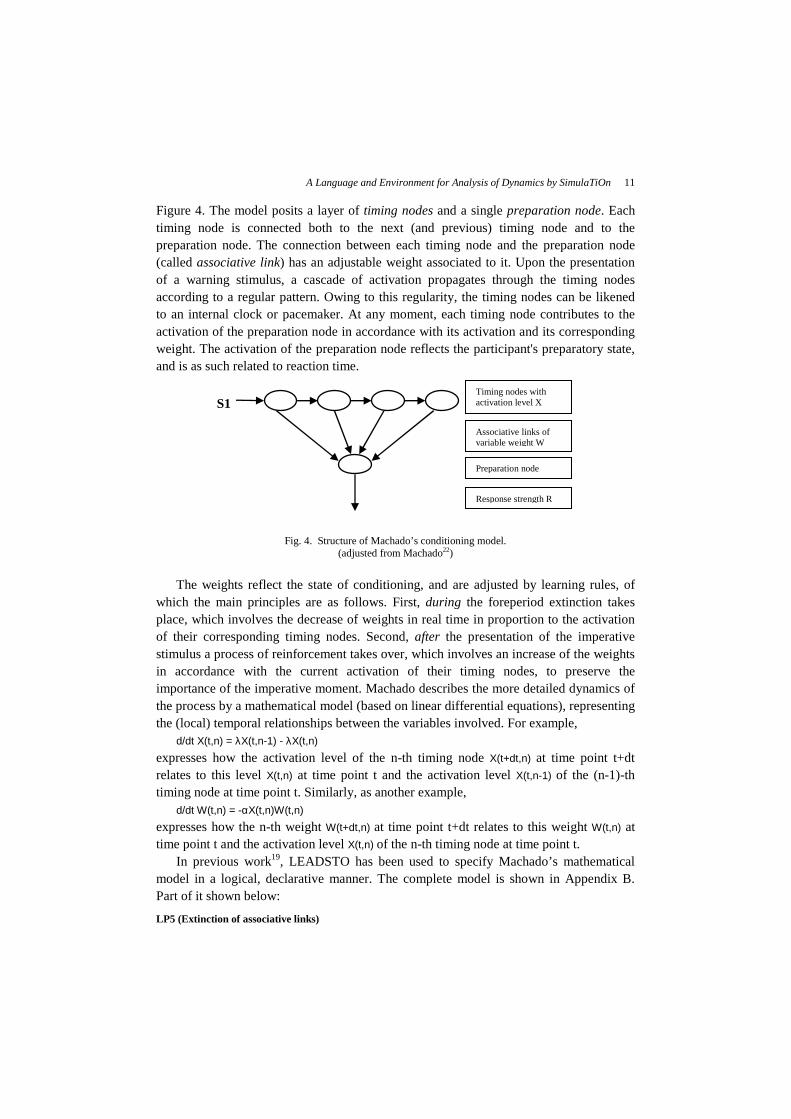
Machado developed a basic model that describes the dynamics of these conditioning processes in terms of differential equations22. The structure of this model is shown in


11

Figure 4. The model posits a layer of timing nodes and a single preparation node. Each timing node is connected both to the next (and previous) timing node and to the preparation node. The connection between each timing node and the preparation node (called associative link) has an adjustable weight associated to it. Upon the presentation of a warning stimulus, a cascade of activation propagates through the timing nodes according to a regular pattern. Owing to this regularity, the timing nodes can be likened to an internal clock or pacemaker. At any moment, each timing node contributes to the activation of the preparation node in accordance with its activation and its corresponding weight. The activation of the preparation node reflects the participant's preparatory state, and is as such related to reaction time.

Fig. 4. Structure of Machado’s conditioning model. (adjusted from Machado22)

The weights reflect the state of conditioning, and are adjusted by learning rules, of which the main principles are as follows. First, during the foreperiod extinction takes place, which involves the decrease of weights in real time in proportion to the activation of their corresponding timing nodes. Second, after the presentation of the imperative stimulus a process of reinforcement takes over, which involves an increase of the weights in accordance with the current activation of their timing nodes, to preserve the importance of the imperative moment. Machado describes the more detailed dynamics of the process by a mathematical model (based on linear differential equations), representing the (local) temporal relationships between the variables involved. For example,

d/dt X(t,n) = λX(t,n-1) - λX(t,n) expresses how the activation level of the n-th timing node X(t+dt,n) at time point t+dt relates to this level X(t,n) at time point t and the activation level X(t,n-1) of the (n-1)-th timing node at time point t. Similarly, as another example,

d/dt W(t,n) = -αX(t,n)W(t,n) expresses how the n-th weight W(t+dt,n) at time point t+dt relates to this weight W(t,n) at time point t and the activation level X(t,n) of the n-th timing node at time point t.

In previous work19, LEADSTO has been used to specify Machado’s mathematical model in a logical, declarative manner. The complete model is shown in Appendix B. Part of it shown below:

LP5 (Extinction of associative links)

S1 Timing nodes with activation level X

Preparation node

Associative links of variable weight W

Response strength R


LP5 expresses the adaptation of the associative links during extinction, based on their own previous state and the previous state of the corresponding timing node. Here, α is a learning rate parameter. Formalisation: ∀u,v:REAL ∀n:INTEGER instage(ext) and X(n, u) and W(n, v) →→0,0,1,1 W(n, v*(1-α*u*step))

LP6 (Reinforcement of associative links) LP6 expresses the adaptation of the associative links during reinforcement, based on their own previous state and the previous state of Xcopy. Here, β is a learning rate parameter. Formalisation: ∀u,v:REAL ∀n:INTEGER instage(reinf) and Xcopy(n, u) and W(n, v) →→0,0,1,1 W(n, v*(1-β*u*step) + β*u*step)

LP7 (Persistence of associative links) LP7 expresses the persistence of the associative links at the moments that there is neither extinction nor reinforcement. Formalisation: ∀v:REAL instage(pers) and W(n, v) →→0,0,1,1 W(n, v)

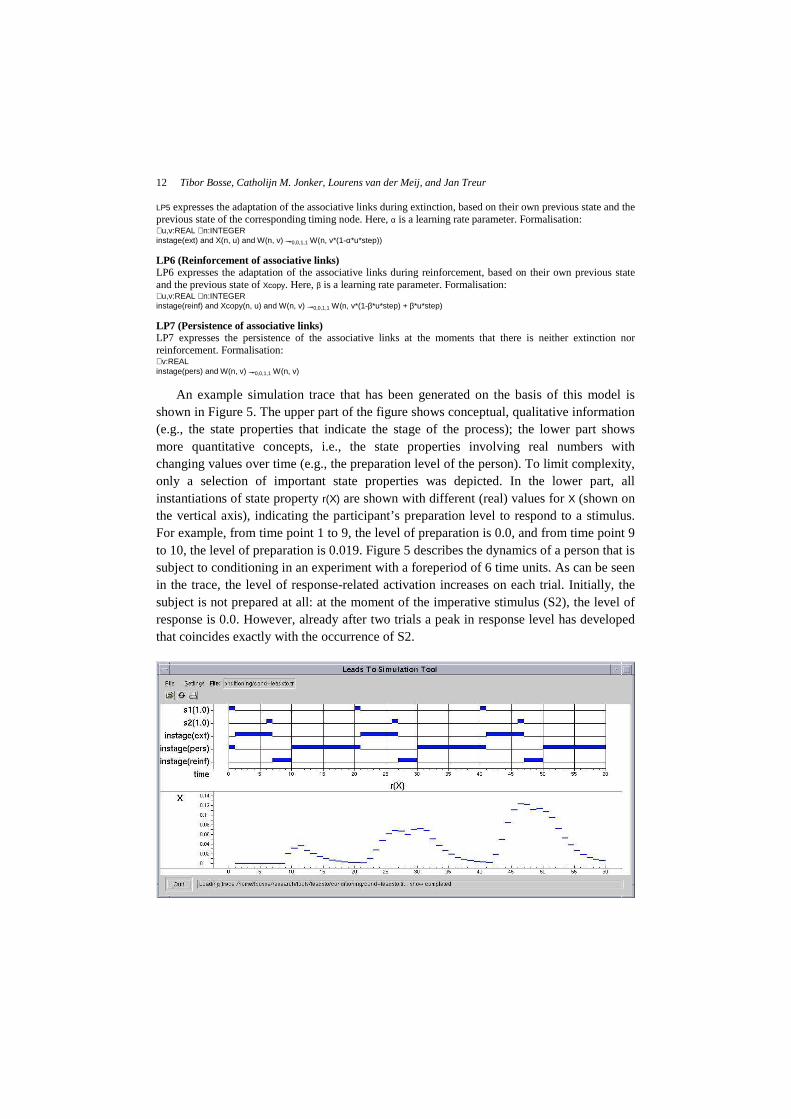
An example simulation trace that has been generated on the basis of this model is shown in Figure 5. The upper part of the figure shows conceptual, qualitative information (e.g., the state properties that indicate the stage of the process); the lower part shows more quantitative concepts, i.e., the state properties involving real numbers with changing values over time (e.g., the preparation level of the person). To limit complexity, only a selection of important state properties was depicted. In the lower part, all instantiations of state property r(X) are shown with different (real) values for X (shown on the vertical axis), indicating the participant’s preparation level to respond to a stimulus. For example, from time point 1 to 9, the level of preparation is 0.0, and from time point 9 to 10, the level of preparation is 0.019. Figure 5 describes the dynamics of a person that is subject to conditioning in an experiment with a foreperiod of 6 time units. As can be seen in the trace, the level of response-related activation increases on each trial. Initially, the subject is not prepared at all: at the moment of the imperative stimulus (S2), the level of response is 0.0. However, already after two trials a peak in response level has developed that coincides exactly with the occurrence of S2.


13

e6

e9

e7

e10

e8

e5

e4 e3 e2

e1

A

B C D

F

E

H G

Fig. 5. Example simulation trace of a conditioning process.

3.3. Ant Colonies

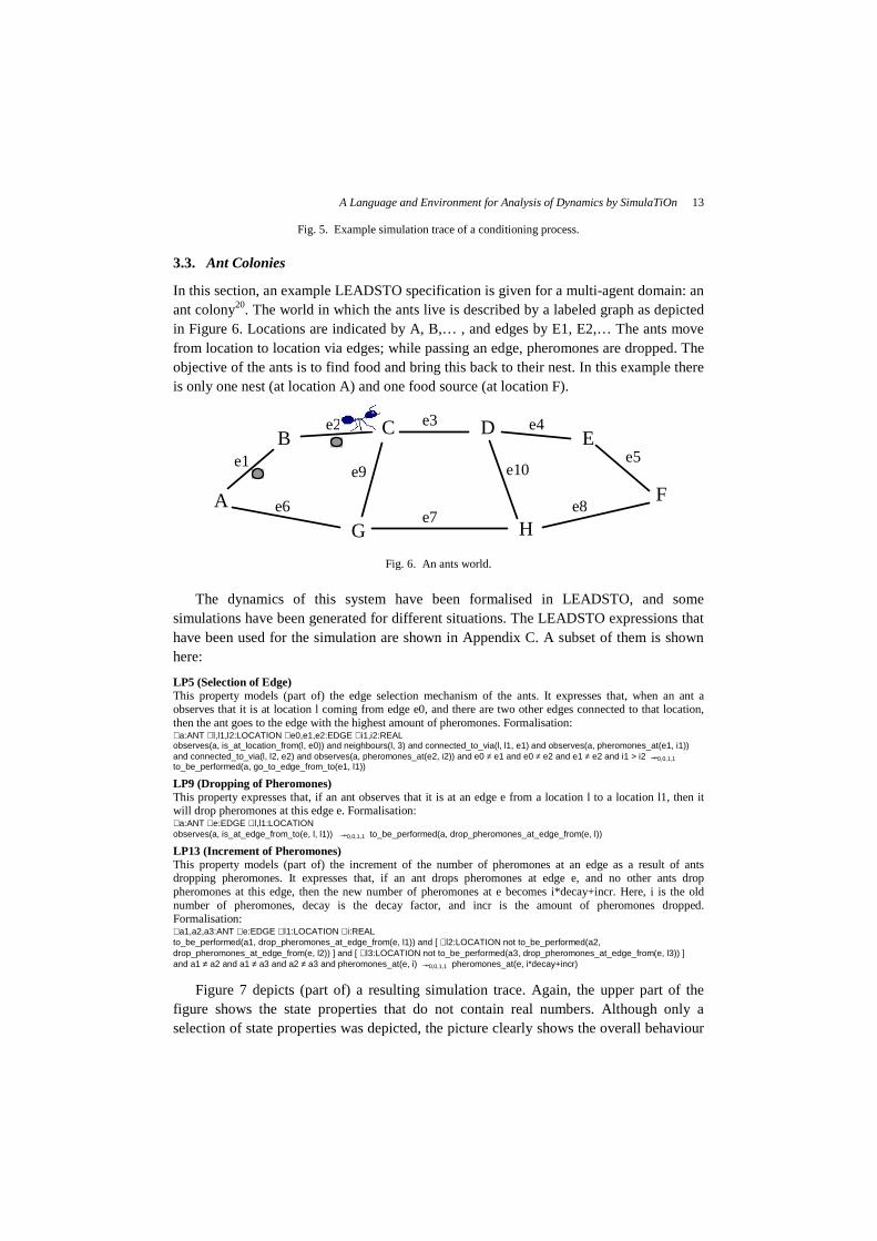
In this section, an example LEADSTO specification is given for a multi-agent domain: an ant colony20. The world in which the ants live is described by a labeled graph as depicted in Figure 6. Locations are indicated by A, B,… , and edges by E1, E2,… The ants move from location to location via edges; while passing an edge, pheromones are dropped. The objective of the ants is to find food and bring this back to their nest. In this example there is only one nest (at location A) and one food source (at location F).

Fig. 6. An ants world.

The dynamics of this system have been formalised in LEADSTO, and some simulations have been generated for different situations. The LEADSTO expressions that have been used for the simulation are shown in Appendix C. A subset of them is shown here:

LP5 (Selection of Edge) This property models (part of) the edge selection mechanism of the ants. It expresses that, when an ant a observes that it is at location l coming from edge e0, and there are two other edges connected to that location, then the ant goes to the edge with the highest amount of pheromones. Formalisation: ∀a:ANT ∀l,l1,l2:LOCATION ∀e0,e1,e2:EDGE ∀i1,i2:REAL observes(a, is_at_location_from(l, e0)) and neighbours(l, 3) and connected_to_via(l, l1, e1) and observes(a, pheromones_at(e1, i1)) and connected_to_via(l, l2, e2) and observes(a, pheromones_at(e2, i2)) and e0 ≠ e1 and e0 ≠ e2 and e1 ≠ e2 and i1 > i2 →→0,0,1,1 to_be_performed(a, go_to_edge_from_to(e1, l1))

LP9 (Dropping of Pheromones) This property expresses that, if an ant observes that it is at an edge e from a location l to a location l1, then it will drop pheromones at this edge e. Formalisation: ∀a:ANT ∀e:EDGE ∀l,l1:LOCATION observes(a, is_at_edge_from_to(e, l, l1)) →→0,0,1,1 to_be_performed(a, drop_pheromones_at_edge_from(e, l))

LP13 (Increment of Pheromones) This property models (part of) the increment of the number of pheromones at an edge as a result of ants dropping pheromones. It expresses that, if an ant drops pheromones at edge e, and no other ants drop pheromones at this edge, then the new number of pheromones at e becomes i*decay+incr. Here, i is the old number of pheromones, decay is the decay factor, and incr is the amount of pheromones dropped. Formalisation: ∀a1,a2,a3:ANT ∀e:EDGE ∀l1:LOCATION ∀i:REAL to_be_performed(a1, drop_pheromones_at_edge_from(e, l1)) and [ ∀l2:LOCATION not to_be_performed(a2, drop_pheromones_at_edge_from(e, l2)) ] and [ ∀l3:LOCATION not to_be_performed(a3, drop_pheromones_at_edge_from(e, l3)) ] and a1 ≠ a2 and a1 ≠ a3 and a2 ≠ a3 and pheromones_at(e, i) →→0,0,1,1 pheromones_at(e, i*decay+incr)

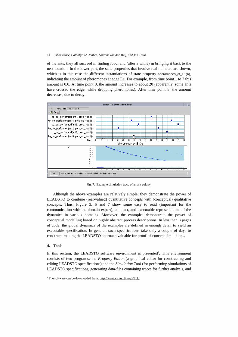
Figure 7 depicts (part of) a resulting simulation trace. Again, the upper part of the figure shows the state properties that do not contain real numbers. Although only a selection of state properties was depicted, the picture clearly shows the overall behaviour


of the ants: they all succeed in finding food, and (after a while) in bringing it back to the nest location. In the lower part, the state properties that involve real numbers are shown, which is in this case the different instantiations of state property pheromones_at_E1(X), indicating the amount of pheromones at edge E1. For example, from time point 1 to 7 this amount is 0.0. At time point 8, the amount increases to about 20 (apparently, some ants have crossed the edge, while dropping pheromones). After time point 8, the amount decreases, due to decay.

Fig. 7. Example simulation trace of an ant colony.

Although the above examples are relatively simple, they demonstrate the power of LEADSTO to combine (real-valued) quantitative concepts with (conceptual) qualitative concepts. Thus, Figure 3, 5 and 7 show some easy to read (important for the communication with the domain expert), compact, and executable representations of the dynamics in various domains. Moreover, the examples demonstrate the power of conceptual modelling based on highly abstract process descriptions. In less than 3 pages of code, the global dynamics of the examples are defined in enough detail to yield an executable specification. In general, such specifications take only a couple of days to construct, making the LEADSTO approach valuable for proof-of-concept simulations.

4. Tools

In this section, the LEADSTO software environment is presenteda. This environment consists of two programs: the Property Editor (a graphical editor for constructing and editing LEADSTO specifications) and the Simulation Tool (for performing simulations of LEADSTO specifications, generating data-files containing traces for further analysis, and a The software can be downloaded from: http://www.cs.vu.nl/~wai/TTL.


15

showing traces). Although the syntax of LEADSTO has already been introduced in Section 2, the LEADSTO software environment uses a slightly different representation. Section 4.1 describes this representation in detail. Next, Section 4.2 introduces the Property Editor and Section 4.3 deals with the Simulation Tool. Section 4.4 describes the algorithm used to generate simulations. Finally, Section 4.5 provides some implementation details and discusses possible improvements for the future.

4.1. LEADSTO Language

This section describes the syntactic representation of LEADSTO specifications, as used within the software environment. Moreover, some additional constructs are introduced, that can be used when performing simulation.

Variables. The language uses typed variables in various constructs. A variable is represented as <Var-Name>’:’<Sort>.

Sorts. Sorts may be defined as a set of instances that may be specified: ‘sortdef(‘<Sort-Name>’,[‘<Terms>’])’, where

<Terms> := <Term>{‘,’<Term>}*

There are also built-in sorts such as integer, real, and ranges of integers represented as, for example, between(2,10).

Atoms. Atoms may be terms built up from names with argument lists where each argument must be a term or a variable, for example: belief(x:AGENT, food_present).

LEADSTO rules. LEADSTO rules are introduced in Section 2. They are represented as: ‘leadsto([‘<Vars>’],‘<Antecedent-Formula>’,‘<Consequent-Formula>’,‘<Delay>’)’, where

<Delay> := ‘efgh(‘<E-Range>’,‘<F-Range>’,‘<G-Range>’,‘<H-Range>’)’b

<Vars> := [<Variable>{‘,’<Variable>}*]

For example, α →→0, 0, 1, 1 β is represented as leadsto([], alfa, beta, efgh(0,0,1,1)). Variables occurring in LEADSTO rules must be explicitly declared as <Variable> entries.

Formulae. LEADSTO rules contain formulae. The current implementation allows conjunctions of atoms or negated atoms and universal quantification over typed variables. Some variables are global, encompassing the whole rule. Other - local - variables are part of universal quantification of some conjunction. The first kind of variables may be of infinite types. Currently, local variables must be of finite types. Some restrictions that are currently applied – such as not allowing disjunction in the antecedents of LEADSTO rules – will be removed in a next version. This will have no effect on the performance of the algorithm discussed in Section 4.4, but will make the details of the algorithm more complex. Other restrictions with respect to variables of infinite type will remain.

Time/Range. Time and Range values occurring in LEADSTO rules and holds_during_interval constructs may be any number or expression evaluating to a number.

b The reason for grouping the delay is to make it easier to use delay constants.


Fig. 8. The LEADSTO property editor

Constants. Constants may be defined using the following construct: ‘constant(‘<Name>’,‘<Value>’)’ A constant(C1, a(1)) entry in a specification will lead to C1 being substituted by a(1) everywhere in the specification.

Intervals. During simulation, some atom values will be derived from LEADSTO rules. Other atoms are not defined by rules but represent constant values of atoms over a certain time range (see Section 2.1). They are expressed as follows: ‘holds_during_interval([‘<Vars>’],‘<Range>’,‘<LiteralConjunction>’)’ In a similar manner, periodically reoccurring constant values are represented as follows: ‘holds_periodically([‘<Vars>’],‘<Range>’,‘<Period>’,‘<LiteralConjunction>’)’, where

<Range> := ‘range(‘<Start-Time>’,‘<End-Time>’)’

<Vars> := [<Variable>{‘,’<Variable>}*]

<Period> : an expression or constant or variable representing a number. <LiteralConjunction> := <Literal> | ‘and(‘<Literals>’)’

<Literals> := <Literal>{‘,’<Literal>}+

<Literal> := <Atom> | {‘not(‘<Atom>’)’}

For example, an entry holds_during_interval([X:between(1,2)], range(10,20), a(X)) makes a(1) and a(2) true in the time range (10,20). Likewise, an entry holds_periodically([], range(0,1),

10, and(p,q)) makes p and q true in time ranges (0,1), (10,11), (20,21), and so on.

Simulation range. The time range over which the simulation must be run is expressed by means of the constructs ’start_time(‘<Time>’)’ and ’end_time(‘<Time>’)’.

Visualisation of Traces. The construct ’display(‘<Tag-Name>’,‘<Property>’)’ is used to specify details of how to display the traces. The <Tag-Name> argument makes it possible to define multiple views of a trace. The active view may be specified from within the User Interface of the Simulation Tool. A number of properties may be specified, for showing or hiding certain atoms, for sorting atoms, for displaying atoms containing numbers within a graph (such as in Figure 5 and 7, lower part), and so on.

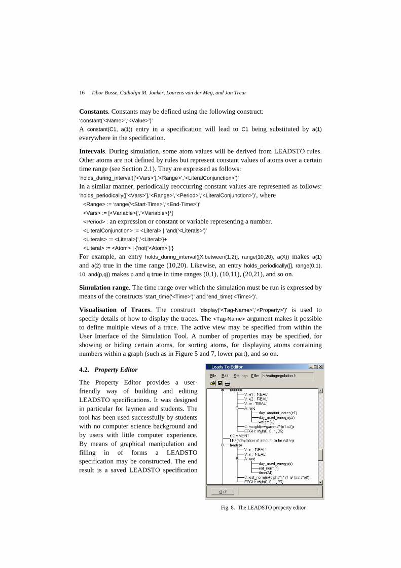
4.2. Property Editor

The Property Editor provides a user-friendly way of building and editing LEADSTO specifications. It was designed in particular for laymen and students. The tool has been used successfully by students with no computer science background and by users with little computer experience. By means of graphical manipulation and filling in of forms a LEADSTO specification may be constructed. The end result is a saved LEADSTO specification


17

file, containing entries discussed in section 4.1. Figure 8 gives an example of how LEADSTO specifications are presented and may be edited with the Property Editor. This screenshot corresponds to the specification described in Section 3.1.

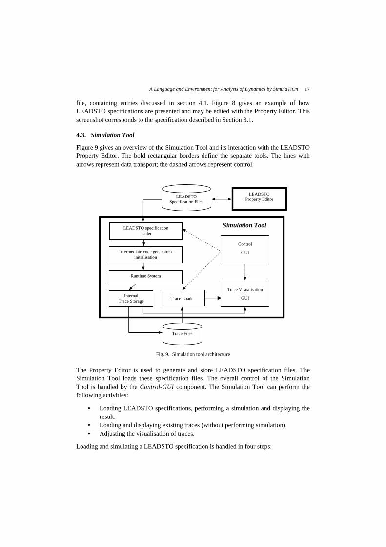
4.3. Simulation Tool

Figure 9 gives an overview of the Simulation Tool and its interaction with the LEADSTO Property Editor. The bold rectangular borders define the separate tools. The lines with arrows represent data transport; the dashed arrows represent control.

Fig. 9. Simulation tool architecture

The Property Editor is used to generate and store LEADSTO specification files. The Simulation Tool loads these specification files. The overall control of the Simulation Tool is handled by the Control-GUI component. The Simulation Tool can perform the following activities:

• Loading LEADSTO specifications, performing a simulation and displaying the result.

• Loading and displaying existing traces (without performing simulation). • Adjusting the visualisation of traces.

Loading and simulating a LEADSTO specification is handled in four steps:

Trace Files

Internal Trace Storage

Trace Visualisation

GUI

Trace Loader

Control

GUI

LEADSTO Property Editor

Simulation Tool

Intermediate code generator / initialisation

Runtime System

LEADSTO Specification Files

LEADSTO specification loader


1. The Specification Loader loads the specification. 2. The Intermediate Code Generator initialises the trace situation with values

defined by holds_during_interval and holds_periodically entries in the specification. The LEADSTO rules are preprocessed: constants are substituted, universal quantifications are expanded and the rules are partially compiled into Prolog calls.

3. The actual simulation is performed by the Runtime System. This is the part that contains the algorithm, discussed in the next section.

4. At the end of a simulation the result is stored internally by the Internal Trace Storage component. The result can be saved as a trace file containing the evolution over time of truth values of all atoms occurring in the simulation, and will be visualised by the Trace Visualisation GUI. In principle, traces are three-valued, using the truth values true, false, and unknown. Saved trace files can be inspected later by the simulation tool and can be used by other tools, e.g., for automated analysis.

Note that visualisation of traces is integrated into the Simulation Tool through the Trace Visualisation GUI component. It is possible to select what atoms must be shown and in what order (sorting). Figure 3, 5 and 7 are examples of the visualisation of the result of a simulation.

4.4. Simulation Engine Algorithm

In this section a sketch of the simulation algorithm is given. The core of the semantics is determined by the LEADSTO rules, for example leadsto(alpha, beta, efgh(e, f, g, h)) or (in the notation of Section 2) α →→e, f, g, h β. The state properties α, β are internally normalised. Currently, only state properties that can be simplified to conjunctions of literals are allowed.

Restrictions on delays. The parameters g and h are time intervals, they must be >= 0. The algorithm allows only causal rules, e,f >= 0. Allowing e,f < 0 would lead to non-causal behaviour (any trace situation could have an effect arbitrarily in the past) and an awkward simulation algorithm. We also restrict ourselves to rules with e + h > 0. The causal nature of the semantics of LEADSTO rules results in a straightforward algorithm: at each time point, a bound part of the past of the trace (the maximum of all g values of all rules) determines the values of a bound range of the future trace (extending at most into the future the maximum of f + h over all LEADSTO rules).

Outline of the algorithm. First all holds_during_interval and holds_periodically entries are handled by setting the ranges of atoms according to their definition. Next, for the algorithm a time variable HandledTime defining an invariant is introduced: this is a time point for which all LEADSTO rules have been dealt with for all α values in time intervals up to and including the interval [HandledTime – g, HandledTime). This implies that for any such interval, for any LEADSTO rule, if α holds, all atoms in the β conjunction have


19

been set in an interval of length h, with a delay between e and f. The idea is to propagate HandledTime until HandledTime >= EndTimec via the following steps:

1. At a certain HandledTime, a value for NextTime is calculated. This will be the first time after HandledTime on which firing of a LEADSTO rule with its g-interval (see Figure 1) extending past HandledTime may have an effect. The time increment will be at least as big as the minimum of e + h over all LEADSTO rules, which is a constant value > 0 as we required e + h > 0. Because we maintain information for each rule regarding up to which antecedent time they have been dealt with, NextTime will often lie further in the future than the minimum of e + h. (Allowing e + h = 0 would complicate the algorithm as we would need to apply some satisfiability solver algorithm).

2. An (optional) Closed World Assumption is performed for all selected atoms in the range [HandledTime, NextTime), i.e., all unknown atoms in this range are made false.

3. All LEADSTO rules are applied for which the range of their antecedent ends before or overlaps with NextTime. In this step we use Prolog unification for the variables occurring in the antecedent and backtracking over all time intervals overlapping with the range [HandledTime, NextTime) matching antecedent literals. As mentioned before, we only allow variables of infinite type within one universal quantification over whole LEADSTO rules, so that Prolog (with its unification and backtracking) can deal with themd. The procedure here is somewhat more complex than Prolog resolution, because while finding matching intervals in the conjunction, an overall interval within which all (negated) atoms of the antecedent hold needs to be maintained.

4. Set HandledTime := NextTime. 5. Continue with step 1 until HandledTime >= EndTime.

4.5. Implementation Details

The complexity of the current algorithm is proportional to the number of LEADSTO rules in the specification, to the number of incremental time steps of the algorithm (which is at most equal to the length of the simulation divided by the minimum of e + h over all LEADSTO rules) and (at most) to the number of matching antecedent atoms per LEADSTO rule (limited by the number of atoms set during the simulation). A number of optimizations already improve the performance, such as only considering antecedent atoms that have matching values in the [HandledTime, NextTime) time range and not considering LEADSTO rules that have been tested to not fire until some time in the future.

c EndTime is the time up to which the simulation should be run. d Other quantification operations over finite types are allowed, but LEADSTO rules containing such quantifications will have those quantifications expanded.


The software was written in SWI-Prolog/XPCE, and consists of approximately 20000 lines of code. The approach for the design and implementation has been to first focus on a complete implementation that is easily adaptable, with acceptable performance for the current users. For an impression of the performance: the simulation of Section 3.1 took two seconds on a regular Personal Computer (processor: 2.2 GHz, memory: 1GB RAM). More complex LEADSTO simulations have been created that take about half an hour to run. For example: one simulation with 170 LEADSTO rules, 2000 time steps, with 15000 atoms set, took 45 minutes.

There is room for further performance improvement of the algorithm. One possible improvement is to increase the time increment NextTime – HandledTime introduced in the algorithm above. Global analysis of dependency of LEADSTO rules should improve the performance, for instance by trying to eliminate simple rules with small values of their e

+ h parameters. Furthermore, the LEADSTO language is being extended with constructs for probabilistic rules, and with constructs for systematically generating traces of LEADSTO specifications for a range of parameters.

5. Related Work

In the literature, a number of modelling approaches exist that have similarities to the approach discussed in this paper. Firstly, there is the family of approaches based on differential and difference equations3, 8, 9. In these approaches, to simulate processes by mathematical means, difference equations are used, for example, of the form: ∆x = f(x) ∆t

or x(t + ∆t) = x(t) + f(x(t)) ∆t. This can be modelled in the LEADSTO language as follows (where d is ∆t): has_value(x, v) →→d, d, d, d has_value(x, v+f(v)*d). This shows how the LEADSTO modelling language subsumes modelling approaches based on difference equations. In addition to those approaches the LEADSTO language allows to express qualitiative and logical aspects.

Another family of modelling approaches, among which approaches based on Executable Temporal Logic1, 5, 6, 7, 14, 15, 16, 17, such as METATEM4, 13, is based on temporal logic formulae of the form ϕ & χ � ψ, where ϕ is a past formula, χ a present formula and ψ a future formula. In comparison to this format, the LEADSTO format is more expressive in the sense that it allows order-sorted predicate logic for state properties, and allows one to express quantitative aspects. Moreover, the explicitly expressed timing parameters (by real numbers) go beyond Executable Temporal Logic and METATEM, which use dicrete time. On the other hand, within some of these approaches it is allowed to refer to past states at different points in time, and thus to model more complex relationships over time. For the LEADSTO language the choice has been made to model only the basic mechanisms of a process (e.g., the direct causal relations), like in modelling approaches based on difference equations and not the more complex ones, but still allowing to express the timing by real numbers.

The Duration Calculus23 is a modal logic for describing and reasoning about the real-time behaviour of dynamic systems, where states change over time and are represented by functions from time (reals) to the Boolean values (0 and 1). It is an extension of


21

Interval Temporal Logic24, but with continuous time, and uses integrated durations of states as interval temporal variables. Assuming finite variability of state functions (i.e., between any two time points only a finite number of state changes), the axioms and rules of Duration Calculus constitute a complete logic (relative to Interval Temporal Logic). A number of interesting tools have been created around (subsets of) Duration Calculus, see, e.g., the work of Pandya25 for information on model checking duration calculus formulae. Duration Calculus itself is not directly used for creating executable models, but environments for executable code exist (e.g., PLC automata26) for which a semantics is given in Duration Calculus.

Another family of modelling approaches based on causal relations is the class of qualitative reasoning techniques2. The main idea of these approaches is to represent quantitative knowledge in terms of abstract, qualitative concepts. Like the LEADSTO language, qualitative reasoning can be used to perform simulation. A difference with LEADSTO is that it is a purely qualitative approach, and that it is less expressive with respect to temporal and quantitative aspects.

Also in the medical domain, modelling dynamics processes by means of causal relations is very common. According to Greenland27, there are currently four major classes of causal models in the health-sciences literature: causal diagrams, potential-outcome models, structural equation models, and sufficient-component cause models. However, as opposed to the work presented in this paper, these approaches only focus on analysis, not on simulation.

Other work that relates qualitative modelling to quantitative modelling can be found in28. This is interesting work that addresses in much depth the question how accurately qualitative models can approximate quantitative models for the same phenomenon. A number of interesting results have been found. A major difference between this work and our work is that we did not (yet) address the question of how qualitative and quantitative models compare, whereas they did address this question in an impressive manner. Instead, our focus has been (up till now) on hybrid modelling, where aspects of a phenomenon that have a quantitative character are modelled in a numerical manner, for example, by differential or difference equations, aspects with a qualitative character are modelled in a logical manner, and both are integrated, as extension of each other. The question what can be done in cases that both would be possible for the same aspect has not been addressed yet in our work. In future work this will be addressed, with the reference as mentioned as a point of departure.

6. Conclusion and Future Work

This article presents the language and software environment LEADSTO that has been developed especially to model and simulate dynamics in terms of both qualitative and quantitative concepts. It is, for example, possible to model differential and difference equations, and to combine those with discrete qualitative modelling approaches. Existing languages are either not accompanied by a software environment that allows simulation


of the model, or do not allow the combination of both qualitative and quantitative concepts.

The language LEADSTO is a declarative order-sorted temporal language extended with quantitative notions (like integer, and real). Time is considered linear, continuous, described by real values. Dynamics can be modelled in LEADSTO as evolution of states over time; i.e., by modelling the direct temporal dependencies between state properties in successive states. The use of durations in these temporal properties facilitates the modelling of such temporal dependencies. In principle, accurately modelling the dynamics of processes may require the use of a dense notion of time, instead of the more practiced variants of discrete time. The problem in a dense time frame of having an infinite number of time points between any two time points is tackled in LEADSTO by the assumption of “Finite Variability”, see, Section 5 and, e.g., the work by Zhou et al.23. Furthermore, main advantages of the LEADSTO language are that it is executable and allows for graphical representation.

The software environment LEADSTO is developed especially for the language. It features a dedicated property editor that proved its value for laymen, students and expert users. The core component is the simulation tool that performs simulations of LEADSTO specifications, generates data-files containing traces of simulation for further analysis, and constructs visual representations of traces. The software environment offers many predefined constructs (e.g., mathematical sorts and operations, intervals and operations thereon).

The approach proved its value in a number of research projects in different domains. It has been used to analyse and simulate behavioural dynamics of agents in cognitive science (e.g., human reasoning29, trace conditioning19, diagnosis of eating disorders18), biology (e.g., cell decision processes30, the dynamics of the heart31), social science (e.g., organisation dynamics including organisational change32, incident management33), and artificial intelligence (e.g., design process34, ant colony behaviour20). As shown by these examples, LEADSTO can be used to model phenomena from diverse perspectives. It has, for example, been used to model cognitive processes from a psychological/BDI perspective and from a physical/neurological perspective.

With respect to future work, it is planned to extend the LEADSTO environment at a number of aspects. Besides some obvious next steps (such as further improving the efficiency of the simulation algorithm and offering some more user-friendly options for debugging), an interesting direction for further research, which is currently explored, is to add non-determinism to LEADSTO specifications. This mainly implies allowing disjunctions within the consequents of LEADSO rules, combined with a probability distribution over the different possibilities. Another possible extension is to create a tool that automatically converts LEADSTO specification to the graphical format depicted in Figure 2.

Acknowledgements


23

The authors are grateful to Martine Delfos, Sander Los, Martijn Schut and Leon van der Torre for their contributions to the simulation models described in Section 3, and to Alexei Sharpanskykh for his contribution to some of the formal details.

References

1. Barringer, H., Fisher, M., Gabbay, D., Owens, R., and Reynolds, M. The Imperative Future: Principles of Executable Temporal Logic, Research Studies Press Ltd. and John Wiley & Sons, 1996.

2. Forbus, K.D. Qualitative process theory. Artificial Intelligence, volume 24, number 1-3, 1984, pp. 85-168.

3. Port, R.F., and Gelder, T. van (eds.). Mind as Motion: Explorations in the Dynamics of Cognition. MIT Press, Cambridge, Mass, 1995.

4. Fisher, M. METATEM: The Story so Far. In: Proceedings of the Third International Workshop on Programming Multi-Agent Systems, ProMAS’03. Lecture Notes in Artificial Intelligence, vol. 3862. Springer Verlag, 2005, pp. 3-22.

5. Fisher, M. (2005). Temporal Development Methods for Agent-Based Systems, Journal of Autonomous Agents and Multi-Agent Systems, vol. 10, pp. 41-66.

6. Galton, A. (2003). Temporal Logic. Stanford Encyclopedia of Philosophy, URL: http://plato.stanford.edu/entries/logic-temporal/#2.

7. Galton, A. (2006). Operators vs Arguments: The Ins and Outs of Reification. Synthese, vol. 150, 2006, pp. 415-441.

8. Kelso, J.A.S. (1995). Dynamic Patterns: the Self-Organisation of Brain and Behaviour. MIT Press, Cambridge, Mass.

9. Ashby, W.R. (1952). Design for a Brain. Chapman & Hall, London. Revised edition 1960. 10. Meyer, J.J.Ch., and Treur, J. (volume eds.) Agent-based Defeasible Control in Dynamic

Environments. Series in Defeasible Reasoning and Uncertainty Management Systems (D. Gabbay and Ph. Smets, series eds.), vol. 7. Kluwer Academic Publishers, 2002.

11. Manzano, M. Extensions of First Order Logic, Cambridge University Press, 1996. 12. Blamey, S. Partial Logic, in: D. Gabbay and F. Guenthner (eds.), Handbook of Philosophical

Logic, Vol. III, 1-70, Reidel, Dordrecht, 1986. 13. Barringer, H., Fisher, M., Gabbay, D., Owens, R., and Reynolds, M. METATEM: A framework

for programming in temporal logic. In: Proceedings of the REX Workshop on Stepwise Refinement of Distributed Systems: Models, Formalisms, Correctness. Lecture Notes in Computer Science, vol. 430. Springer Verlag, 1989, pp. 94-129.

14. Fisher, M. (1997). A Normal Form for Temporal Logics and its Applications in Theorem-Proving and Execution. Journal of Logic and Computation, vol. 7, 1997, pp. 429-456.

15. Gabbay, D.M. (1989). The Declarative Past and Imperative Future: Executable Temporal Logic for Interactive Systems. In B. Banieqbal, H. Barringer, and A. Pnueli, (eds), Proceedings of the 1st Conference on Temporal Logic in Specification. Lecture Notes in Computer Science, vol. 398. Springer Verlag, 1989, pp. 409-448.

16. Gabbay, D.M., Hodkinson, I., Reynolds, M. (1994). Temporal Logic: Mathematical and Computational Aspects, Vol. 1. Clarendon Press, Oxford, 1994.

17. Hodkinson, I., and Reynolds, M. (2005). Separation - Past, Present and Future. In: We Will Show Them: Essays in Honour of Dov Gabbay, Vol 2. S. Artemov, H. Barringer, A. S. d'Avila Garcez, L. C. Lamb, and J. Woods (eds.), pp. 117-142, College Publications, 2005.

18. Bosse, T., Delfos, M.F., Jonker, C.M., and Treur, J. Analysis of Adaptive Dynamical Systems for Eating Regulation Disorders. Proceedings of the 25th Annual Conference of the Cognitive Science Society, CogSci 2003. Mahwah, NJ: Lawrence Erlbaum Associates, Inc., 2003, pp.


168-173. Extended version in: Simulation Journal: Transactions of the Society for Modeling and Simulation International, volume 82, issue 3, 2006, pp. 159-171.

19. Bosse, T., Jonker, C.M., Los, S.A., Torre, L. van der, and Treur, J. Formalisation and Analysis of the Temporal Dynamics of Conditioning. In: Mueller, J.P. and Zambonelli, F. (eds.), Proceedings of the Sixth International Workshop on Agent-Oriented Software Engineering, AOSE'05, pp. 157-168, 2005. Extended version will appear in: Cognitive Systems Research Journal.

20. Bosse, T., Jonker, C.M., Schut, M.C., and Treur, J. Simulation and Analysis of Shared Extended Mind. In: Davidsson, P., Gasser, L., Logan, B., and Takadama, K. (eds.), Proc. of the Joint Workshop on Multi-Agent and Multi-Agent-Based Simulation, MAMABS'04. Lecture Notes in AI, vol. 3415, Springer Verlag, 2005, pp. 248-264. Extended version in: Simulation Journal: Transactions of the Society for Modeling and Simulation International, volume 81, issue 9, 2005, pp. 719-732.

21. Delfos, M.F. Lost Figure: Treatment of Anorexia, Bulimia and Obesitas (in Dutch). Swets and Zeitlinger Publishers, Lisse, 2002.

22. Machado, A. Learning the Temporal Dynamics of Behaviour. Psychological Review, vol. 104, 1997, pp. 241-265.

23. Zhou, C., Hoare, C.A.R., and Ravn, A.P. A Calculus of Durations, Information Processing Letter, 40, 5, 1991, pp. 269-276.

24. Moszkowski, B., and Manna, Z. Reasoning in Interval Temporal Logic. In Clarke, E., and Kozen, D., editors, Proceedings of the Workshop on Logics of Programs, volume 164 of LNCS, pp. 371-382, Pittsburgh, PA, June 1983. Springer Verlag.

25. Pandya, P.K., Model checking CTL[DC]. In: Proceedings of TACAS 2001, Genova, LNCS 2031, Springer-Verlag, April 2001. Also as Technical Report TCS-00-PKP-2, Tata Institute of Fundamental Research, Mumbai, 2000. http://www.tcs.tifr.res.in/~pandya/dcvalid103.html.

26. Dierks, H. PLC-automata: A new class of implementable real-time automata. In: M. Bertran and T. Rus, editors, Transformation-Based Reactive Systems Development (ARTS'97), volume 1231 of Lecture Notes in Computer Science, pp. 111-125. Springer-Verlag, 1997.

27. Greenland, S., and Brumback, B.A. An overview of relations among causal modeling methods. International Journal of Epidemiology, 31, pp. 1030-1037, 2002.

28. Berleant, D., and Kuipers, B. Qualitative and quantitative simulation: bridging the gap. Artificial Intelligence Journal, vol. 95, issue 2, 1997, pp. 215-255.

29. Bosse, T., Jonker, C.M., and Treur, J. Reasoning by Assumption: Formalisation and Analysis of Human Reasoning Traces. In: Mira, J., Alvarez, J.R. (eds.), Proc. of the First International Work-conference on the Interplay between Natural and Artificial Computation, IWINAC'05. Lecture Notes in Artificial Intelligence, vol. 3561. Springer Verlag, 2005, pp. 430-439. Extended version in: Cognitive Science Journal, volume 30, issue 1, 2006, in press.

30. Jonker, C.M., Snoep, J.L., Treur, J., Westerhoff, H.V., and Wijngaards, W.C.A. Putting Intentions into Cell Biochemistry: An Artificial Intelligence Perspective. Journal of Theoretical Biology, vol. 214, 2002, pp. 105-134.

31. Bosse, T., Jonker, C.M., and Treur, J. Organisation Modelling for the Dynamics of Complex Biological Processes. In: G. Lindemann, D. Moldt, M. Paolucci, B. Yu (eds.), Regulated Agent-Based Social Systems, Proc. of the International Workshop on Regulated Agent-Based Social Systems: Theories and Applications, RASTA'02. Lecture Notes in AI, vol. 2934. Springer Verlag, 2004, pp. 92-112.

32. Hoogendoorn, M., Jonker, C.M., Schut, M., and Treur, J. Modelling the Organisation of Organisational Change. In: Giorgini, P., and Winikoff, M., (eds.), Proceedings of the Sixth International Bi-Conference Workshop on Agent-Oriented Information Systems (AOIS'04), 2004, pp. 29-46.


25

33. Hoogendoorn, M., Jonker, C.M., Popova, V., Sharpaskykh, A., Xu, L. Formal Modelling and Comparing of Disaster Plans. In: Carle, B., and Walle, B. van de, (eds.), Proceedings of the Second International Conference on Information Systems for Crisis Response and Management ISCRAM '05, 2005, pp. 97-107.

34. Bosse, T., Jonker, C.M., and Treur, J. Analysis of Design Process Dynamics. In: R. Lopez de Mantaras, L. Saitta (eds.), Proceedings of the 16th European Conference on Artificial Intelligence, ECAI'04, 2004, pp. 293-297.


Appendix A. Simulation Model for Eating Regulation Example LP1 (Eat-stimulus) The first local property LP1 expresses that an eat norm N and an intermediate amount eaten E less than this norm together lead to an eat stimulus. Formalisation: ∀E,N:REAL intermediate_amount_eaten(E) and eat_norm(N) and E < N →→0,0,1,1 stimulus(eat)

LP2 (Not-eat-stimulus) Local property LP2 expresses that an eat norm N and an intermediate amount eaten E higher than this norm together lead to an non-eat stimulus. Formalisation: ∀E,N:REAL intermediate_amount_eaten(E) and eat_norm(N) and E ≥ N →→0,0,1,1 stimulus(do_not_eat)

LP3 (Increase of amount eaten) Local property LP3 expresses how an eat stimulus increases an intermediate amount eaten by additional energy d (the energy value of what is eaten). Formalisation: ∀E:REAL intermediate_amount_eaten(E) and stimulus(eat) →→0,0,1,1 intermediate_amount_eaten(E+d)

LP4 (Stabilizing amount eaten) Local property LP4 expresses how a non-eat stimulus keeps the intermediate amount eaten the same. Formalisation: ∀E:REAL intermediate_amount_eaten(E) and stimulus(do_not_eat) →→0,0,1,1 intermediate_amount_eaten(E)

LP5 (Day amount eaten) Local property LP5 expresses that the day amount eaten is the intermediate amount eaten at the end of the day. Formalisation: ∀E:REAL intermediate_amount_eaten(E) and time(24) →→0,0,1,1 day_amount_eaten(E)

LP6 (Weight through balance of amount eaten and energy used) Local property LP6 expresses a simple mechanism of how weight is affected by the day balance of amount eaten and energy used. Here γ is a fraction that specifies how energy leads to weight kilograms. Formalisation: ∀E1,E2,W:REAL day_amount_eaten(E1) and day_used_energy(E2) and weight(W) →→0,0,1,25 weight(W + γ * (E1 – E2))

LP7 (Adaptation of amount to be eaten) Local property LP7 expresses a simple (logistic) mechanism for the adaptation of the eat norm based on the day amount of energy used. Here α is the adaptation speed, β is the fraction of E that is the limit of the adaptation; normally β = 1. Formalisation: ∀E,N:REAL day_used_energy(E) and eat_norm(N) and time(24) →→0,0,1,25 eat_norm(N + α * N * (1 - N/βE))

LP8 (Recent weight) Local property LP8 expresses that if the current weight is W, then in the near future the recent weight will be W. Formalisation: ∀W:REAL weight(W) →→25,25,25,25 recent_weight(W)

LP9 (Indication of anorexia) Local property LP9 expresses that if the difference between the current weight and the recent weight is more than δ, then there is an indication that the patient has anorexia. Formalisation: ∀W1,W2:REAL weight(W1) and recent_weight(W2) and W1-W2 > δ →→0,0,1,1 indication(anorexia)

LP10 (Indication of obesitas) Local property LP10 expresses that if the difference between the recent weight and the current weight is more than ε, then there is an indication that the patient has obesitas. Formalisation: ∀W1,W2:REAL weight(W1) and recent_weight(W2) and W2-W1 > ε →→0,0,1,1 indication(obesitas)


27

Appendix B. Simulation Model for Conditioning Example LP1 (Initialisation) The first local property LP1 expresses the initialisation of the values for the timing nodes and the associative links. Formalisation (for n ranging over [0,5]): ∀n:INTEGER start →→0,0,1,1 X(n, 0) and W(n, 0)

LP2 (Activation of initial timing nodes) Local property LP2 expresses the activation (and adaptation) of the 0th timing node. Immediately after the occurrence of the warning stimulus (S1), this state has full strength. After that, its value decreases until the next warning stimulus. Together with LP3, this property causes the spread of activation across the timing nodes. Here, λ > 0 is a rate parameter that controls the speed of this spread of activation, and step is a constant indicating the smallest time step in the simulation. For the simulation experiments described in this paper, λ was set to 10 and step was set to 0.05. Formalisation: ∀u,s:REAL X(0, u) and S1(s) →→0,0,1,1 X(0, u*(1-λ*step)+s)

LP3 (Adaptation of timing nodes) LP3 expresses the adaptation of the nth timing node (for n ranging over [1,5]), based on its own previous state and the previous state of the n-1th timing node. Together with LP2, this property causes the spread of activation across the timing nodes. Here, λ is a rate parameter that controls the speed of this spread of activation (see LP2). Formalisation: ∀n:INTEGER ∀u0,u1:REAL X(n, u1) and X(n-1, u0) →→0,0,1,1 X(n, u1+λ*(u0-u1)*step)

LP4 (Storage of timing nodes at moment of reinforcer) LP4 is needed to store the value of the nth timing node at the moment of the occurrence of the imperative stimulus (S2). These values are used later on by property LP6. Formalisation: ∀n:INTEGER ∀x:REAL X(n, u) and S2(1.0) →→0,0,1,3 Xcopy(n, u)

LP5 (Extinction of associative links) LP5 expresses the adaptation of the associative links during extinction, based on their own previous state and the previous state of the corresponding timing node. Here, α is a learning rate parameter. Formalisation: ∀u,v:REAL ∀n:INTEGER instage(ext) and X(n, u) and W(n, v) →→0,0,1,1 W(n, v*(1-α*u*step))

LP6 (Reinforcement of associative links) LP6 expresses the adaptation of the associative links during reinforcement, based on their own previous state and the previous state of Xcopy. Here, β is a learning rate parameter. Formalisation: ∀u,v:REAL ∀n:INTEGER instage(reinf) and Xcopy(n, u) and W(n, v) →→0,0,1,1 W(n, v*(1-β*u*step) + β*u*step)

LP7 (Persistence of associative links) LP7 expresses the persistence of the associative links at the moments that there is neither extinction nor reinforcement. Formalisation: ∀v:REAL instage(pers) and W(n, v) →→0,0,1,1 W(n, v)

LP8 (Response function) LP8 calculates the response by adding the discriminative function of all states (i.e., their associative links * the degree of activation of the corresponding state). Formalisation: ∀v1,v2,v3,v4,v5,u1,u2,u3,u4,u5:REAL W(1, v1) and W(2, v2) and W(3, v3) and W(4, v4) and W(5, v5) and X(1, u1) and X(2, u2) and X(3, u3) and X(4, u4) and X(5, u5) →→0,0,1,1 R(v1*u1 + v2*u2 + v3*u3 + v4*u4 + v5*u5)

LP9 (Initialisation of stage pers) LP9 expresses that the initial stage of the process is pers. Formalisation: start →→0,0,1,1 instage(pers)

LP10 (Transition to stage ext) LP10 expresses that the process switches to stage ext when a warning stimulus occurs. Formalisation: S1(1.0) →→0,0,1,1 instage(ext)

LP11 (Persistence of stage ext)


LP11 expresses that the process persists in stage ext as long as no imperative stimulus occurs. Formalisation: instage(ext) and S2(0.0) →→0,0,1,1 instage(ext)

LP12 (Transition to stage reinf and pers) LP12 expresses that the process first switches to stage reinf for a while, and then to stage pers when an imperative stimulus occurs. Notice that LP12a and LP12b must have different timing parameters to make sure both stages do not occur simultaneously. Formalisation: S2(1.0) →→0,0,1,3 instage(reinf) (LP12a) S2(1.0) →→3,3,1,1 instage(pers) (LP12b)

LP13 (Persistence of stage pers) LP13 expresses that the process persists in stage pers as long as no warning stimulus occurs. Formalisation: instage(pers) and S1(0.0) →→0,0,1,1 instage(pers)


29

Appendix C. Simulation Model for Ants Example LP1 (Initialisation of Pheromones) This property expresses that at the start of the simulation, at all edges there are 0 pheromones. Formalisation: start →→0,0,1,1 pheromones_at(E1, 0.0) and pheromones_at(E2, 0.0) and pheromones_at(E3, 0.0) and pheromones_at(E4, 0.0) and pheromones_at(E5, 0.0) and pheromones_at(E6, 0.0) and pheromones_at(E7, 0.0) and pheromones_at(E8, 0.0) and pheromones_at(E9, 0.0) and pheromones_at(E10, 0.0)

LP2 (Initialisation of Ants) This property expresses that at the start of the simulation, all ants are at location A. Formalisation: start →→0,0,1,1 is_at_location_from(ant1, A, init) and is_at_location_from(ant2, A, init) and is_at_location_from(ant3, A, init)

LP3 (Initialisation of World) These two properties model the ants world. The first property expresses which locations are connected to each other, and via which edges they are connected. The second property expresses for each location how many neighbours it has. Formalisation: start →→0,0,1,1 connected_to_via(A, B, l1) and … and connected_to_via(D, H, l10)

start →→0,0,1,1 neighbours(A, 2) and … and neighbours(H, 3)

LP4 (Initialisation of Attractive Directions) This property expresses for each ant and each location, which edge is most attractive for the ant at if it arrives at that location. This criterion can be used in case an ant arrives at a location where there are two edges with an equal amount of pheromones. Formalisation: start →→0,0,1,1 attractive_direction_at(ant1, A, E1) and … and attractive_direction_at(ant3, E, E5)

LP5 (Selection of Edge) These properties model the edge selection mechanism of the ants. For example, the first property expresses that, when an ant observes that it is at location A, and both edges connected to location A have the same number of pheromones, then the ant goes to its attractive direction. Formalisation: ∀a:ANT ∀l1,l2:LOCATION ∀e0,e1,e2:EDGE ∀i1,i2:REAL observes(a, is_at_location_from(A, e0)) and attractive_direction_at(a, A, e1) and connected_to_via(A, l1, e1) and observes(a, pheromones_at(e1, i1)) and connected_to_via(A, l2, e2) and observes(a, pheromones_at(e2, i2)) and e1 \= e2 and i1 = i2 →→0,0,1,1 to_be_performed(a, go_to_edge_from_to(e1, A, l1))

∀a:ANT ∀l1,l2:LOCATION ∀e0,e1,e2:EDGE ∀i1,i2:REAL observes(a, is_at_location_from(A, e0)) and connected_to_via(A, l1, e1) and observes(a, pheromones_at(e1, i1)) and connected_to_via(A, l2, e2) and observes(a, pheromones_at(e2, i2)) and i1 > i2 →→0,0,1,1 to_be_performed(a, go_to_edge_from_to(e1, A, l1))

∀a:ANT ∀l1,l2:LOCATION ∀e0,e1,e2:EDGE ∀i1,i2:REAL observes(a, is_at_location_from(F, e0)) and connected_to_via(F, l1, e1) and observes(a, pheromones_at(e1, i1)) and connected_to_via(F, l2, e2) and observes(a, pheromones_at(e2, i2)) and i1 > i2 →→0,0,1,1 to_be_performed(a, go_to_edge_from_to(e1, F, l1))

∀a:ANT ∀l,l1:LOCATION ∀e0,e1:EDGE observes(a, is_at_location_from(l, e0)) and neighbours(l, 2) and connected_to_via(l, l1, e1) and e0 ≠ e1 and l ≠ A and l ≠ F →→0,0,1,1

to_be_performed(a, go_to_edge_from_to(e1, l, l1))

∀a:ANT ∀l,l1,l2:LOCATION ∀e0,e1,e2:EDGE observes(a, is_at_location_from(l, e0)) and attractive_direction_at(a, l, e1) and neighbours(l, 3) and connected_to_via(l, l1, e1) and observes(a, pheromones_at(e1, 0.0)) and connected_to_via(l, l2, e2) and observes(a, pheromones_at(e2, 0.0)) and e0 ≠ e1 and e0 ≠ e2 and e1 ≠ e2 →→0,0,1,1 to_be_performed(a, go_to_edge_from_to(e1, l, l1))

∀a:ANT ∀l,l1,l2:LOCATION ∀e0,e1,e2:EDGE ∀i1,i2:REAL observes(a, is_at_location_from(l, e0)) and neighbours(l, 3) and connected_to_via(l, l1, e1) and observes(a, pheromones_at(e1, i1)) and connected_to_via(l, l2, e2) and observes(a, pheromones_at(e2, i2)) and e0 ≠ e1 and e0 ≠ e2 and e1 ≠ e2 and i1 > i2 →→0,0,1,1 to_be_performed(a, go_to_edge_from_to(e1, l1))

LP6 (Arrival at Edge) This property expresses that, if an ant goes to an edge e from a location l to a location l1, then later the ant will be at this edge e. Formalisation: ∀a:ANT ∀e:EDGE ∀l,l1:LOCATION to_be_performed(a, go_to_edge_from_to(e, l, l1)) →→0,0,1,1 is_at_edge_from_to(a, e, l, l1)

LP7 (Observation of Edge) This property expresses that, if an ant is at a certain edge e, going from a location l to a location l1, then it will observe this. Formalisation: ∀a:ANT ∀e:EDGE ∀l,l1:LOCATION is_at_edge_from_to(a, e, l, l1) →→0,0,1,1 observes(a, is_at_edge_from_to(e, l, l1))

LP8 (Movement to Location)


This property expresses that, if an ant observes that it is at an edge e from a location l to a location l1, then it will go to location l1. Formalisation: ∀a:ANT ∀e:EDGE ∀l,l1:LOCATION observes(a, is_at_edge_from_to(e, l, l1)) →→0,0,1,1 to_be_performed(a, go_to_location_from(l1, e))

LP9 (Dropping of Pheromones) This property expresses that, if an ant observes that it is at an edge e from a location l to a location l1, then it will drop pheromones at this edge e. Formalisation: ∀a:ANT ∀e:EDGE ∀l,l1:LOCATION observes(a, is_at_edge_from_to(e, l, l1)) →→0,0,1,1 to_be_performed(a, drop_pheromones_at_edge_from(e, l))

LP10 (Arrival at Location) This property expresses that, if an ant goes to a location l from an edge e, then later it will be at this location l. Formalisation: ∀a:ANT ∀e:EDGE ∀l:LOCATION to_be_performed(a, go_to_location_from(l, e)) →→0,0,1,1 is_at_location_from(a, l, e)

LP11 (Observation of Location) This property expresses that, if an ant is at a certain location l, then it will observe this. Formalisation: ∀a:ANT ∀e:EDGE ∀l:LOCATION is_at_location_from(a, l, e) →→0,0,1,1 observes(a, is_at_location_from(l, e))

LP12 (Observation of Pheromones) This property expresses that, if an ant is at a certain location l, then it will observe the number of pheromones present at all edges that are connected to location l. Formalisation: ∀a:ANT ∀e0,e1:EDGE ∀l,l1:LOCATION ∀i:REAL is_at_location_from(a, l, e0) and connected_to_via(l, l1, e1) and pheromones_at(e1, i) →→0,0,1,1 observes(a, pheromones_at(e1, i))

LP13 (Increment of Pheromones) These properties model the increment of the number of pheromones at an edge as a result of ants dropping pheromones. For example, the first property expresses that, if an ant drops pheromones at edge e, and no other ants drop pheromones at this edge, then the new number of pheromones at e becomes i*decay+incr. Here, i is the old number of pheromones, decay is the decay factor, and incr is the amount of pheromones dropped. Formalisation: ∀a1,a2,a3:ANT ∀e:EDGE ∀l1:LOCATION ∀i:REAL to_be_performed(a1, drop_pheromones_at_edge_from(e, l1)) and [ ∀l2:LOCATION not to_be_performed(a2, drop_pheromones_at_edge_from(e, l2)) ] and [ ∀l3:LOCATION not to_be_performed(a3, drop_pheromones_at_edge_from(e, l3)) ] and a1 ≠ a2 and a1 ≠ a3 and a2 ≠ a3 and pheromones_at(e, i) →→0,0,1,1 pheromones_at(e, i*decay+incr)

∀a1,a2,a3:ANT ∀e:EDGE ∀l1,l2:LOCATION ∀i:REAL to_be_performed(a1, drop_pheromones_at_edge_from(e, l1)) and to_be_performed(a2, drop_pheromones_at_edge_from(e, l2)) and [ ∀l3:LOCATION not to_be_performed(a3, drop_pheromones_at_edge_from(e, l3)) ] and a1 ≠ a2 and a1 ≠ a3 and a2 ≠ a3 and pheromones_at(e, i) →→0,0,1,1 pheromones_at(e, i*decay+incr+incr)

∀a1,a2,a3:ANT ∀e:EDGE ∀l1,l2,l3:LOCATION ∀i:REAL to_be_performed(a1, drop_pheromones_at_edge_from(e, l1)) and to_be_performed(a2, drop_pheromones_at_edge_from(e, l2)) and to_be_performed(a3, drop_pheromones_at_edge_from(e, l3)) and a1 ≠ a2 and a1 ≠ a3 and a2 ≠ a3 and pheromones_at(e, i) →→0,0,1,1 pheromones_at(e, i*decay+incr+incr+incr)

LP14 (Collecting of Food) This property expresses that, if an ant observes that it is at location F (the food source), then it will pick up some food. Formalisation: ∀a:ANT ∀e:EDGE ∀l:LOCATION observes(a, is_at_location_from(l, e)) and food_location(l) →→0,0,1,1 to_be_performed(a, pick_up_food)

LP15 (Carrying of Food) This property expresses that, if an ant picks up food, then as a result it will be carrying food. Formalisation: ∀a:ANT to_be_performed(a, pick_up_food) →→0,0,1,1 is_carrying_food(a)

LP16 (Dropping of Food) This property expresses that, if an ant is carrying food, and observes that it is at location A (the nest), then the ant will drop the food. Formalisation: ∀a:ANT ∀e:EDGE ∀l:LOCATION observes(a, is_at_location_from(l, e)) and nest_location(l) and is_carrying_food(a) →→0,0,1,1 to_be_performed(a, drop_food)

LP17 (Persistence of Food) This property expresses that, as long as an ant that is carrying food does not drop the food, it will keep on carrying it. Formalisation:


31

∀a:ANT is_carrying_food(a) and not to_be_performed(a, drop_food) →→0,0,1,1 is_carrying_food(a)

LP18 (Decay of Pheromones) This property expresses that, if the old amount of pheromones at an edge is i, and there is no ant dropping any pheromones at this edge, then the new amount of pheromones at e will be i*decay. Formalisation: ∀e:EDGE ∀i:REAL pheromones_at(e, i) and [ ∀a:ANT ∀l:LOCATION not to_be_performed(a, drop_pheromones_at_edge_from(e, l)) ] →→0,0,1,1 pheromones_at(e, i*decay)

Documents

A LANGUAGE AND ENVIRONMENT FOR ANALYSIS OF DYNAMICS …wai/Papers/IJAIT07leadsto.pdf · A Language and Environment for Analysis of Dynamics by SimulaTiOn 5 Fig. 2. Example of a graphical