A level-set approach for the metamorphosis of solid …david/Papers/TVCG_morph.pdf · associated with morphing 3D shapes rather than 2D images, ... The level-set approach to 3D model

A Level-Set Approach for theMetamorphosis of Solid Models

David E. Breen, Member, IEEE Computer Society, and Ross T. Whitaker, Member, IEEE

AbstractÐThis paper presents a new approach to 3D shape metamorphosis. We express the interpolation of two shapes as a process

where one shape deforms to maximize its similarity with another shape. The process incrementally optimizes an objective function

while deforming an implicit surface model. We represent the deformable surface as a level set (iso-surface) of a densely sampled

scalar function of three dimensions. Such level-set models have been shown to mimic conventional parametric deformable surface

models by encoding surface movements as changes in the grayscale values of a volume data set. Thus, a well-founded mathematical

structure leads to a set of procedures that describes how voxel values can be manipulated to create deformations that are represented

as a sequence of volumes. The result is a 3D morphing method that offers several advantages over previous methods, including

minimal need for user input, no model parameterization, flexible topology, and subvoxel accuracy.

Index TermsÐLevel set method, morphing, solid model, distance function, animation, volume graphics, optimization, deformable

model.

æ

1 INTRODUCTION

SHAPE metamorphosis is a process where an objectcontinuously changes its own shape into the shape of

another object. Within the computer graphics community,morphing (the vernacular for metamorphosis) has been usedfrequently for special effects in movies, advertising, andentertainment. Image morphing takes a 2D image of an objectand transforms the appearance of that object into theappearance of another object, with the goal of producingnatural-appearing, or at least sensible, intermediate images.Three-dimensional morphing or shape morphing involvessmoothly changing the model of one object into the modelof another object. Shape morphing algorithms have beendeveloped for both surface models and volumetric models.The surface model algorithms transform the surface patches(usually polygons) of the source model into the surfacepatches of the target model. The volume-based morphingalgorithms represent 3D objects as volumes and manipulatethe voxel values of volumes in order to make one objectbecome another. Volume data sets needed for this processmay be acquired directly from 3D scanning devices, such asMRI or CT, or they may be generated via 3D scanconversion of solid geometric models.

Despite the increased complexity and computation time

associated with morphing 3D shapes rather than 2D images,

shape morphing does have some distinct advantages. First,

image morphing is directly tied to the views of the two

input images. Any morphing effect must be based only on

the information available in the two images. This preventsthe animator from making camera, lighting, or shadingchanges during the morph. If the morph is performed with3D techniques, the animator is provided with much moreflexibility in presenting the results of the morph. Once asequence of transforming models has been generated, theanimator may experiment with a variety of camera anglesand motions for viewing the models. The scene's globallighting and shading parameters may also change duringthe morph. A second advantage is that a 3D morph ensuresthat the resulting rendered images represent a continuoussequence of actual 3D shapes. In image morphing, main-taining the 3D feasibility of the intermediate images is theresponsibility of the user, i.e., care must be taken to makesure intermediate images represent pictures of feasibleobjects rather than a fuzzy mixture of ghost-like objects.

One disadvantage of 3D morphing is that it requires two3D models. It is not always possible to acquire accuratemodels of the objects that one wishes to morph, e.g., asequence of familiar faces. At present, digital photographsof real objects tend to capture more visual detail than3D models of the same. Despite this, there is a class ofmorphing problems for which 3D models exist or are easilyobtainable which lend themselves to the application ofshape morphing.

In order to compare the adequacy of different ap-proaches to 3D shape morphing, we have identified severaldesirable aspects of a 3D morphing technology. Theseproperties are:

1. The transition process should begin with a sourcesurface and end with a specified target surface.

2. Intermediate surfaces should undergo continuous3D transitions (rather than continuity only in theimage space).

3. The morphing algorithm should apply to a widerange of shapes and topologies.

IEEE TRANSACTIONS ON VISUALIZATION AND COMPUTER GRAPHICS, VOL. 7, NO. 2, APRIL-JUNE 2001 173

. D.E. Breen is with the Computer Graphics Laboratory, MS 348-74,California Institute of Technology, Pasadena, CA 91125.E-mail: [email protected].

. R.T. Whitaker is with the School of Computing, 3450 Merrill EngineeringBldg., University of Utah, Salt Lake City, UT 84112-9205.E-mail: [email protected].

Manuscript received 29 Oct. 1999; revised 29 June 2000; accepted 19 Oct.2000.For information on obtaining reprints of this article, please send e-mail to:[email protected], and reference IEEECS Log Number 110869.

1077-2626/01/$10.00 ß 2001 IEEE

4. A 3D morphing algorithm should incorporate userinput easily but should degrade gracefully without it.

5. Transitional shapes should depend only on thesurface geometry of the two input shapes and userinput.

These requirements are not exhaustive, but they capturemany of the practical aspects of 3D morphing.

In this paper, we present a new approach to 3D modelmorphing. We employ an active deformable surface whichstarts at the source shape and smoothly changes into thetarget shape. This deformation process is described by theoptimization of an objective function that measures thesimilarity between the target and the deforming surface. Werepresent the deformable surface as a level set (iso-surface)of a densely sampled scalar function of three dimensions.The sampling produces a regularly spaced rectilinearvolume data set. Such level-set models [37], [41] have beenshown to mimic conventional parametric deformable sur-face models by encoding surface movements as changes inthe grayscale values of the volume. A well-foundedmathematical structure leads to a set of procedures thatdescribes how voxel values can be manipulated to createdeformations in the level sets. The result is a voxel-basedmodeling technology that offers several advantages overprevious methods, including support for a wide range ofuser input, no need for parameterization, flexible topology,and subvoxel accuracy. This paper describes the applicationof this technology to 3D surface morphing.

This work, as with several other volumetric morphingtechniques [11], [26], is based on the image morphingstrategy and consists of two distinct steps. The first step is aglobal, geometric warping, which utilizes a coordinatetransformation that maps the source model into approxi-mately the same shape and orientation as the target model,as shown in Fig. 1. This coordinate transformation can takea variety of different forms, but the literature has shownthat a rigid transformation combined with a nonrigid,spline-based, coordinate map is quite effective. The non-rigid transformation is usually determined by a set of user-defined correspondences (i.e., fiducials) between the sourceimage/volume and the target. The second step is a blendingthat completes the morph by ensuring that any discrepan-cies that remain in the images/volumes after the warping

are gradually removed over the course of the morphingprocess. In image morphing and volumetric shape morph-ing, the blending step is usually achieved by a simple linearinterpolation, or cross-dissolve, of the two images/volumes.The warping stage of image/volume morphing has beenstudied extensively by other researchers and our workprimarily focuses on developing a superior method for theblending stage, one which reduces the amount of user inputrequired to produce an acceptable morphing result. Indeed,the proposed level-set approach to shape metamorphosiswill produce a reasonable morph with virtually no userinput. Given this technology, user input can be incorpo-rated in an incremental fashion, starting with a minimalamount and proceeding with progressively more until asatisfactory result is achieved.

Our morphing approach consists of several stages. First,the source and target objects are defined, with ConstructiveSolid Geometry (CSG) models in our examples. The modelsare scan converted into 3D distance volumes (a signeddistance transform), where the shortest distance to the solidmodel is stored at each voxel. We use the sign conventionthat distance is positive inside the object and negativeoutside the object. A level-set model is fit to the zero levelset of the source model distance volume. A coordinatetransformation provides a mapping from every point in thedomain of the level-set model into the distance volume ofthe target model. This is the warping step. The level-setmodel is then allowed to deform using the signed distancetransform of the target model. Each point on the sourcesurface moves in the direction normal to the surface at thatpoint with a velocity proportional to the signed distancetransform of the target object at that point in 3-space. Thisprocess is the blending step of the 3D surface morph. Atuser-defined time intervals, the level-set model is convertedinto a polygonal model. This model is expressed in thecoordinate system of the source model. Therefore, thecoordinate transformation is incrementally applied, as afunction of time, to the sequence of polygonal models,which are then rendered to produce the frames of themorphing animation.

In general, an animator controls the morph by defininghow the models overlap, using a variety of coordinatetransformations. This can include rigid transformations,scalings, and nonrigid transformations determined by setsof user-defined fiducials. Our current implementation alsoprovides an automated mechanism for determining rota-tion, translation, and nonuniform scaling and thereby offersthe option of a totally automatic morphing algorithm. Thesystem accomplishes this by overlaying the centroids of thetwo models, aligning their principal axes, and nonuni-formly scaling along these axes. The surface of the level-setmodel only moves in those areas where the target and thesource surfaces are not brought together perfectly by thecoordinate transformation. The portion of the level-setmodel which is outside of the target model will shrink,while the portion inside the target model will expand tobecome the final shape.

The level-set approach to 3D model morphing providesseveral advantages over other 3D morphing algorithms.Level-set models are active; their underlying motion is

174 IEEE TRANSACTIONS ON VISUALIZATION AND COMPUTER GRAPHICS, VOL. 7, NO. 2, APRIL-JUNE 2001

Fig. 1. Shape morphing, like image morphing, can be described as a

warping combined with a blending.

defined algorithmically rather than interactively, guaran-teeing that the source shape will become the target shape,given that both models initially overlap. The amount of userinput required to produce a morph is directly proportionalto the amount of control the animator wishes to impose onthe process. The animator may allow the system toautomatically generate the morph or he/she can employ afull 3D warping to describe the morph, with the level setssimply providing a small fine-tuning of the surface. Anyintermediate amount of user input will produce a reason-able morph. Because level-set models do not rely on anykind of parameterization, they do not suffer the problems ofparametric surfaces, e.g., a limited set of possible shapesand the need for reparameterization after undergoingsignificant changes in shape. This lack of parameterization,along with no direct representation of topological structure,allow level-set models to easily change topology whilemorphing. The model can ªsplitº into pieces to formmultiple objects. Conversely, several disjoint objects maycome together to make a single object. Finally, both the scanconversion and deformation stages of our morphingapproach produce models with user-defined subvoxelaccuracy. This provides a flexible time-quality trade-offand generates superior results at low volume resolutions ascompared to previous work.

The remainder of the paper proceeds as follows: Section 2describes related morphing work. Section 3 describes thenovel aspect of our methodÐshape interpolation based onthe optimization of a similarity function using level-setmodels. It is followed by a discussion of general propertiesand numerical methods. Section 6 describes all stages of ourmorphing approach. The paper closes with three morphingexamples, conclusions, and some thoughts on future work.

2 RELATED WORK

In recent years, numerous 3D morphing algorithms havebeen reported in the literature. These algorithms generallyfall into two categories, surface-based approaches andvolume-based approaches. The former primarily consistsof those methods that continuously change one polygonalsurface into another. Volumetric methods modify the voxelvalues of a volume data set in order to smoothly transformthe object defined by the volume from a source shape into atarget shape. A third class of algorithms involves morphingimplicit models, either by transforming the underlyingstructure of ªblobbyº models [14] or by creating higherdimensional interpolating implicit functions [39].

Kent et al. [23] described the fundamentals for morphing3D polygonal surfaces. The first step is to create a singletopological description of vertices, edges, and faces whichcontains the combined topological structure of both thesource and target surfaces (the correspondence phase). Thevertices of the structure are then interpolated between theirposition on the initial surface to their position on the targetsurface to create the morphing result. Parent [31] presentsan improved technique for establishing vertex and edgecorrespondences when creating the combined topologicalstructure. Chen et al. [9] applied the same approach topolygonal surfaces defined in cylindrical coordinates. Kanaiet al. [21] use harmonic maps to define the correspondences

in the combined topological structure. Lazarus and Ver-roust [24] do not build a common adjacency graph, butinstead create a common parameterized mesh during asampling process. Gregory et al. [17] present a method toassist the user in defining these correspondences. Lee et al.[25] apply many of these surface-based methods tomorphing multiresolution meshes. Kaul and Rossignac[22], [34] introduce the notion of an interpolating polyhe-dron, an application of mathematical morphology to facesets. They also describe a user control methodology basedon a Bezier curve paradigm. DeCarlo and Gallier [12]demonstrate that it is possible (with significant effort) tomorph polygonal models of differing genus. Surface-basedmethods are important because of the wealth of polygonalmodels available to animators, but they are burdened withthe difficult task of creating a single topological structurewhich can represent the source and target surfaces. While ithas been shown that changing the genus of a morphingpolygonal surface is possible, for example, from a sphere toa torus, it can be a difficult and tedious process whichrequires significant user input. Another troubling feature ofsurface-based methods is the problem of self-intersection.These methods cannot guarantee that polygonal surfaceswill not pass through themselves, creating physicallynonsensical intermediate results.

Embedding the morphing surfaces in volumes alleviatesthese problems. Hughes [19] demonstrates how volumescan be used to create a morph between objects of differentgenus. The approach involves linearly interpolating theFourier transforms of the volumes. A schedule is usedduring interpolation which filters out the high frequenciesof the initial volume while interpolating the low frequenciesof both volumes and gradually adds the high frequencies ofthe target volume. He et al. [18] propose a similar approachusing wavelets to control the high-frequency artifacts. Theyalso developed methods that allow the user some control ofthe interpolation by establishing explicit correspondencesbetween the volumes. Lerios et al. [26] describe a morphingmethod which is a 3D extension of Beier and Neely's [4]2D (image) morphing technique. The first step is to apply auser-defined geometric warp to the source object in order todeform it into approximately the same shape as the targetobject. This step allows the user to specify correspondingfeatures on the two objects. The second step interpolates thevalues between matching voxels in the (warped) source andtarget volumes. Chen et al. [10] propose disk fields as asuperior instrument for specifying the warps needed forthis kind of 3D morphing. Payne and Toga [32] describe amethod for changing one volumetric model into another byinterpolating the distance fields generated from the twovolumes. A distance field, or distance volume, is a volumedata set where the value stored at each voxel is the shortestdistance to the surface of the object being represented by thevolume. Cohen-Or et al. [11] improve upon this approachby including a two-part warping step that calculates a rigidtransformation and an elastic warping based upon user-supplied anchor points. This extra step approximatelyaligns the target and final objects and provides significantuser control to the overall morphing process.

BREEN AND WHITAKER: A LEVEL-SET APPROACH FOR THE METAMORPHOSIS OF SOLID MODELS 175

The proposed volume-based morphing technique sharesmany of the advantages of previous volume-based methods.It can easily morph objects of different genus. It is notburdened with the difficult vertex/edge/face bookkeepingof surface methods and surfaces cannot pass through eachother. Additionally, our method provides a novel blending/interpolation mechanism that will not produce the ghostingor spontaneous generation of new objects which is possiblewhen simply interpolating voxel intensity or distance values(for example, see Figs. 4, 5, and 6). Our method does notrequire user input to produce a reasonable morph, but caneasily incorporate previously published warping techniquesto provide a wide range of animator control. Finally, becausewe calculate the distance transform to subvoxel accuracy andeffectively track a deforming surface within voxels, ourresults do not produce the aliasing artifacts commonly foundin other distance-based, volumetric approaches.

3 METAMORPHOSIS AS A GOAL-DRIVEN PROCESS

Morphing strategies may be built upon any number ofunderlying principles. For instance, surface metamorphosiscould consist of a sequence of time slices from a four-dimensional manifold which optimizes some space-timecriteria [39]. The proposed strategy for object metamorpho-sis is based on yet another principle: Shape metamorphosisis the process by which one object seeks to resemble another.This philosophy raises two questions. First, what is themetric by which we can quantify the similarity of twoobjects? Second, what is the process by which one objectseeks to optimize that metric? This paper shows that evenvery simple answers to these two questions produce verypowerful algorithms for shape metamorphosis, with a greatdeal of opportunity for future enhancement and refinementof the resulting algorithms.

In order to create a very general algorithm for metamor-

phosis, we work with a very general notion of a surface.

Consider an open set A � IR3, which is the source object,

and a target B � IR3. The source, A, is enclosed by a

surface SA � @A and, likewise, SB � @B. We require that

the objects be compact and lie in some finite domain

U � IR3. Notice that we do not require any specific

connectivity or topology, which means that each object

could consist of a set of disconnected pieces (each with any

number of holes) all sitting in U .We propose a very simple metric for comparing two

shapes that maximizes the volume shared by the interiors ofthe two objects. First, define an inside-outside function forthe target, B : IR3 7!IR for B such that

B�x� � 0 8 x 2 SB B�x� > 0 8 x 2 B

B�x� < 0 otherwise:�1�

The inside-outside function B can be used to quantify theextent to which an intermediate object t overlaps with thetarget, B, with the volume integral

MB;t�Z

t

B�x�dx: �2�

Notice, this integral achieves its maximum,

m � arg maxt

Zt

B�x�dx

� �; �3�

when m � B because, in that case, the integral includes

all of the positive parts of B and none of the negative parts.We can compute the first variation of this metric with

respect to t by noting that incremental changes in the

object shape can be expressed in terms of the surface that

encloses it:Zt�dt

B�x�dx �Z

t

B�x�dx�ZSt B�x��x� �N�x�dx;

�4�where N : St 7!S3 is the surface normal, which is a mapping

from every point on the surface to the unit sphere.

Differentiating with respect to � gives the first variation

[13] with respect to surface position:

dM� B�x�N�x�: �5�Using the first variation from (5) and a hill climbing

strategy, we obtain the surface motion, defined for each

surface point, that minimizes our similarity metric:

ds

dt� B s�t�� N s�t�� 8 s�t� 2 St: �6�

This equation states that each point on the surface St moves

at each time step dt in the direction of the surface normal

N s�t�� with a step size proportional to the value of the

inside-outside function B s�t�� at the point location.

4 PROPERTIES

This section describes the properties of the solutions of the

partial differential equation given in (6). For this paper, we

examine the case of simple, closed, surfaces, but the results

easily generalize to more complicated surfaces. In this

section, we systematically show that if the initial and target

objects overlap, the final solution of the metamorphosis will

be identical to the target.

4.1 Steady-State Solution

We begin by examining properties of the steady-state

solution of (6), which is the surface St such that

@s�t�=@t � 0 for all s 2 St. Thus, for steady state, which

we denote S1,

B�x�N�s� � 0) B�s� � 0 8s 2 S1: �7�The inside-outside function for the target, B, has the

property that

B�x� � 0 , x 2 SB: �8�Thus, we can conclude S1 � SB. From this, it follows that if

S1 is compact and closed, it must have one of two forms:

1. S1 � ;,2. S1 � SB.


The first case is trivial because there are no points on S1to violate the condition given in (7). The second case follows

from the fact that simple, closed, connected surfaces have

no proper subsets that are also closed surfaces. Thus,

S1 � SB and S1 closed ) S1 � SB: �9�Also, because the first variation of the metricMB;t

is zero

only where St � SB, it achieves its maximum for that

solution with t � B.Another important aspect of the algorithm is that a

component of the source that overlaps with a component of

the target will deform in such a way that it takes on the

shape of that target component.1 This follows from the fact

that the metricMB;tcan be decomposed into two parts (as

in Fig. 2):

MB;t�Mi

B;t�Mo

B;t�Z

it

B�x� �Z

ot

B�x�; �10�

where it � t \ B and o

t � t ÿ it ÿ SB. In this case, the

first variation produces a pair of deformable surfaces that

share a boundary along t \ SB. The exterior model

remains on the exterior of SB and contracts (increasing

the value of Mo) until it collapses into itself along SB and

the value of Mo reaches zero. The interior model expands,

cannot pass into the exterior of SB and increases the value

of Mi at a rate

@Mi

@t�ZSit B�x�dx: �11�

Because B�x� is nonnegative on the interior of the target,

B, the metric does not stop increasing (and thus the

surface keeps moving) until the surface reaches its steady

state, i.e., B�x� � 0 8 x 2 Sit. Thus, if a source component

overlaps with a target component, the resulting morph does

not terminate until it reaches the shape of the target.

4.2 Strategy

This formulation suggests a strategy for shape metamor-phosis: Construct a family of objects t (with a correspond-ing St), with tjt�0 � A that evolve according to a hill-climbing strategy, and maximize M. If properly initialized(i.e., all of the components of B have some overlap withA), then the deformation will seek the global maximum,which is the target B.

The intermediate shapes contained in t depend, ofcourse, on the choice of B. In order to avoid numericaldifficulties and to avoid discontinuities in the solution, Bshould be continuous.2 Furthermore, B should rewardshapes that are similar to the target but offset by some smalldistance. That is, B should carry information about theshape of the surface into 3D so that shapes tend to ªlooklikeº the target as they get nearer. This suggests that anatural choice of B is the signed distance transform [2], [5] ofthe target surface SB or some monotonic function thereof.Thus, if we let DB : U 7!IR be the signed distance transform, B�x� � f DB�x�� , where f�0� � 0 and f 0�a� > 0. By tuningf , one can control the way the metamorphosis behaveswhen intermediate surfaces are far from the target. Iff�a� � a, then St contracts or expands with a magnitudethat depends on the signed distance to the target.

As it stands, this process is a ªlow-levelº approach toshape metamorphosis, which can form continuous defor-mations for shapes that are somehow ªcloseº in their initialshapes. As described in the introduction, this low-levelprocess is meant to address the blending stage of3D metamorphosisÐit is meant to be combined with ahigher-level process which accounts for ªsemanticº aspectsof shape correspondence. Incorporating user input isimportant for any shape morphing technique because, inmany cases, finding the best set of transition shapesdepends on context. Only users can apply semanticconsiderations to the transformation of one object toanother. Our assertion, however, is that this underlyingcoordinate transformation can achieve only some finite


Fig. 2. In order to see that overlapping models converge, we can divide the model t into two parts separated by a stationary boundary; one part

contracts to annihilation while the other expands until it is equal to the target.

1. A target object may consist of several disjoint components.2. In general, signed distance transforms are C0 continuous, but not C1

continuous.

similarity between the ªwarpedº source model and thetarget and even this may require a great deal of user input.In the event that a user is not able or willing to define everyimportant correspondence between two objects, some othermethod must ªfill inº the gaps remaining between thesource and target surface. We propose the use of deform-able level-set models to achieve a continuous transition(blending) between the shapes that result from the under-lying coordinate transformation.

This higher-level information affects the blending pro-cess through a 3D coordinate transformation, T . T maps apoint x in the coordinate system of the source A into thecoordinate system of the target B. As described in theintroduction, this transformation is meant to be quitegeneral; it can accommodate a wide range of globaldeformations. However, if the blending is sufficientlypowerful and can adequately deal with significant shapediscrepancies (after the coordinate transformation), only acrude alignment of the source and target is necessary. Thecoordinate transformation enters into the deformationprocess through the term B, which quantifies the proximityof one surface to another by means of the distancetransform. If we express the distance transform for thetarget in coordinates of the target, then we have B�x� � f�DB�T �x��. Alternatively, one could resamplethe distance transform of B in the coordinate system of A,i.e., 0B�x� � B�T �x��.

5 LEVEL-SET MODELS

In practice, the strategy of shape metamorphosis by surfacedeformations described in the previous section must becomputed using some specific surface representation.Ideally, we would like the surface representation to be asgeneral as the underlying theory. For this we use themethod of level-set models [37], which is a technique formodeling surfaces as iso-values of a densely sampled scalarfunction over the domain U . Surface movements areencoded as changes in the grayscale values of the voxels.Using level-set models, we can compute goal-drivendeformations on surfaces without any explicit surfacerepresentation.

5.1 Theory

The strategy of level-set models represents a set of surfacepoints S as an iso-surface of �, which we will call theembedding.

S � fxj��x� � kg; �12�where the value of k is arbitrary and will fall out insubsequent calculations.3 We can also represent a family ofsurfaces and a corresponding family of embeddings:

St � fxj��x; t� � kg: �13�Consider a point s�t� on the surface that moves through

space as a function of t. Because s�t� remains the kth level-surface of � over time, the total derivative of � with respectto time must be zero. Thus,

@��s�t�; t�@t

�r��s�t�; t� � ds�t�dt� 0; �14�

which establishes the connection between the way points onSt move and the way the grayscale values (at positions onthe surface) of the embedding change. We can rewrite (14)as follows:

@�

@t� ÿr� � ds�t�

dt� jr�j ds�t�

dt�N�s�; �15�

using the fact that r� � jr�jN.We can now ªplugº into (15) any surface motion we wish

to compute. Thus, inserting ds�t�=dt from (6), whichdescribes the motion of the surface model as it becomesmore like the target, yields

@� s� �@t� jr�j B s�t�� ; �16�

where we have used the fact that surface normal is unitlength, i.e., N �N � 1. Notice, we have not chosen aparticular k and, therefore, this analysis applies to everylevel set of �. Thus, we are describing the deformation of anembedded family of surface models each of which evolvesaccording to the same equation:

@��x�@t

� jr��x�j B�x�: �17�

The particular level set of interest is the one that we choose,by construction of the initial conditions, such that��x; 0� � k 8 x 2 SA.

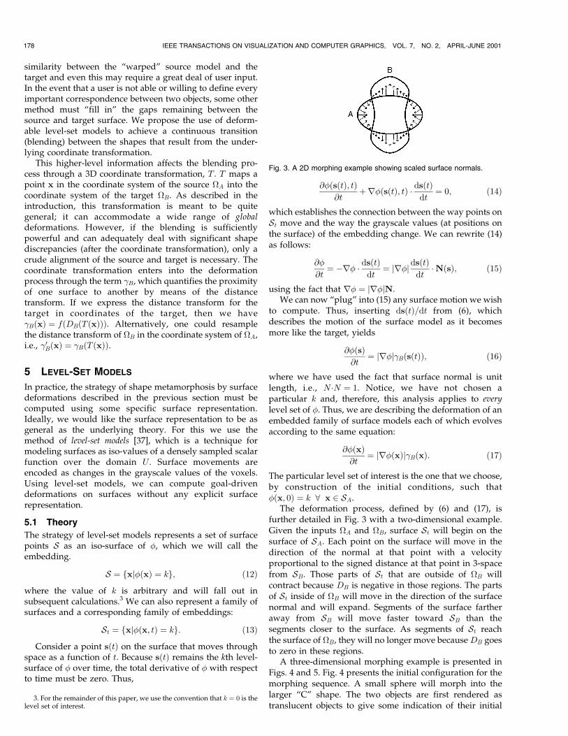
The deformation process, defined by (6) and (17), isfurther detailed in Fig. 3 with a two-dimensional example.Given the inputs A and B, surface St will begin on thesurface of SA. Each point on the surface will move in thedirection of the normal at that point with a velocityproportional to the signed distance at that point in 3-spacefrom SB. Those parts of St that are outside of B willcontract because DB is negative in those regions. The partsof St inside of B will move in the direction of the surfacenormal and will expand. Segments of the surface fartheraway from SB will move faster toward SB than thesegments closer to the surface. As segments of St reachthe surface of B, they will no longer move because DB goesto zero in these regions.

A three-dimensional morphing example is presented inFigs. 4 and 5. Fig. 4 presents the initial configuration for themorphing sequence. A small sphere will morph into thelarger ªCº shape. The two objects are first rendered astranslucent objects to give some indication of their initial


3. For the remainder of this paper, we use the convention that k � 0 is thelevel set of interest.

Fig. 3. A 2D morphing example showing scaled surface normals.

overlap. The ball is mostly contained inside the ªCº shape,

with the light blue regions of the sphere protruding outside

the red ªC.º The morphing sequence in Fig. 5 demonstrates

that the regions outside of the ªCº contract slightly to fit to

the surface of the ªC.º The surface regions of the sphere

inside of the ªCº expand to fill the remainder of the object.

This also demonstrates that having a surface expand in the

direction of its local normal will allow it to deform to fit

concave objects, a fact also shown by Miller et al. [29]. Fig. 6

contrasts our method of blending with the method used in

several other volume-based morphing techniques. Here, the

voxel values of the two initial distance volumes are simply

interpolated. It can be seen that voxel interpolation

produces undesirable artifacts, namely pieces of the ªCº

shape ªpop out of thin air.º This is a typical problem when

using voxel interpolation to blend volumetric objects. In

order to overcome this problem in this example, the sphere

would have to be geometrically warped into approximately

the same shape as the ªC.º Our method requires no

warping. The user specifies the initial overlap of the two

objects and the level-set deformation completes the morph.The complete deformation strategy is as follows: First,

initialize a volume so that the kth level set is, approximately,

aligned with SB. For all of our work, we will use the zero-

set as the level-set model. This initialization can be done by

using the discrete distance transform of SB, which we

compute from CSG models using the method of Breen et al.

[7], [8]. We use this initialization to solve the initial value

problem given by (17), using the distance transform of the

target as the B. We solve this equation using finite forward

differences, as described in the next section. When the

model is sufficiently close to the target (a threshold on the

RMS distance to the target), the process stops and the

metamorphosis is complete.

5.2 Implementation

5.2.1 Numerical Issues

The solutions to the partial differential equations describedin Section 5.1 are computed using finite differences on adiscrete grid.4 The use of a grid and discrete time stepsraises a number of numerical and computational issues thatare important to the implementation.

The first issue is the discrete approximation of thederivatives in (17). Let un be a discrete approximation to��x; t� at the nth discrete time step. The equation can besolved using finite forward differences if one uses the up-wind scheme, proposed by Osher and Sethian [30], tocompute the spatial derivatives. The update equation is

un�1i;j;k � uni;j;k ��t�uni;j;k; �18�

where �t is a constant that is chosen to ensure stability and

�uni;j;k is the discrete approximation to @�=@t. We assume,

without a loss in generality, that the grid spacing is unity.

The initial conditions u0 are established by the algorithm

and the boundary conditions are such that the derivatives

toward the outside of the grid are zero (Neumann type).The up-wind scheme relies on one-side derivatives:

��x uni;j;k � uni�1;j;k ÿ uni;j;k; �19�

�ÿx uni;j;k � uni;j;k ÿ uniÿ1;j;k; �20�

��y uni;j;k � uni;j�1;k ÿ uni;j;k; �21�

�ÿy uni;j;k � uni;j;k ÿ uni;jÿ1;k; �22�

and so forth. The partials in (17) are computed using onlythose derivatives that are up-wind relative to the movementof the level set. Thus, the update becomes

�ui;j;k � B i; j; k� ��Pw2x;y;z min��wuni;j;k; 0�2

��Pw2x;y;z max��ÿwuni;j;k; 0�2

�12

for B�i; j; k� � 0

Pw2x;y;z max��wuni;j;k; 0�2

��Pw2x;y;z min��ÿwuni;j;k; 0�2

�12

for B�i; j; k� < 0:

8>>>>>>>>><>>>>>>>>>:�23�

The time steps, �t, are limited by the speed of the fastestmoving wavefront, which can move only one grid unit periteration, i.e.,

�t � 1

3 maxi;j;k j B�i; j; k�j : �24�

In practice, for the purposes of computer animation, onemight further limit the time steps to obtain sequences with asufficient number of in-between frames.

Thus, the level-set method for computing the 3D shapemetamorphosis is as follows:


Fig. 4. Initial configuration for a morphing sequence.

4. The level-set software used to produce the morphing results in thispaper is available for public use in the VISPACK libraries at http://www.cs.utah.edu/~whitaker/vispack.


Fig. 5. A 3D level-set morphing example.

Fig. 6. Interpolation of two distance volumes.

1. Initialize model volume u0 by sampling the inside-outside function of the source.

2. Construct the volume v by sampling the inside-outside function of the target.

3. vmax � 0.4. For each voxel �i; j; k�:

a. Find vi;j;k.b. vmax �MAX�jvi;j;kj; vmax�.c. Calculate derivatives and the total change at�i; j; k� using nearest neighbors according to theup-wind scheme given in (23).

d. Save �uni;j;k in a separate volume.5. Compute �t according to (24).6. For each voxel �i; j; k�:

a. Update un�1i;j;k according to (18).

b. Compute the stopping criterion, either RMSchange or RMS distance to target.

c. If the stopping criterion is met, finish; otherwise,go to Step 4.

5.2.2 Sparse-Field Solutions

The up-wind solutions to the equations described in theprevious section produce the motion of level-set models overthe entire range of the embedding, i.e., for all values of k in(13). However, this method requires updating every voxel inthe volume for each iteration, which means that the computationtime increases as a function of the volume, rather than thesurface area, of the model. Because the application of thispaper, surface metamorphosis, requires only a single model,the calculation of solutions over the entire range of iso-valuesis an unnecessary computational burden.

The literature has shown this situation can be improvedby the use of narrow-band methods, which computesolutions only in a narrow band of voxels that surroundthe level set of interest [1], [28]. In previous work [40], [42],we described an alternative numerical algorithm, called thesparse-field method, that computes the geometry of only asmall subset of points in the range and requires a fraction ofthe computation time required by previous algorithms. Wehave shown two advantages to this method. The first is asignificant improvement in computation times. The secondis increased accuracy when fitting models to forcingfunctions that are defined to subvoxel accuracy.

The sparse-field algorithm takes advantage of the factthat a k-level surface, S, of a discrete image u (of anydimension) has a set of cells through which it passes, asshown in Fig. 7. The set of grid points adjacent to the levelset is called the active set and the individual elements of thisset are called active points. As a first-order approximation,the distance of the level set from the center of any activepoint is proportional to the value of u divided by thegradient magnitude at that point. We compute the evolu-tion given by (17) on the active set and then update theneighborhood around the active set using a fast approx-imation to the distance transform, which simply adds theªcity-blockº distance to values of the active set. Becauseactive points must be adjacent to the level-set model, theirpositions lie within a fixed distance to the model. Therefore,the values of u for elements in the active set must lie withina certain range of grayscale values. When active-point

values move out of this active range, they are no longeradjacent to the model. They must be removed from the setand other grid points, those whose values are moving intothe active range, must be added to take their place. Theprecise ordering and execution of these operations isimportant to the operation of the algorithm.

The values of the points in the active set can be updatedusing the up-wind scheme described in the previoussection. In order to maintain stability, one must updatethe neighborhoods of active grid points in a way that allowsgrid points to enter and leave the active set without thosechanges in status affecting their values. Grid points shouldbe removed from the active set when they are no longer thenearest grid point to the zero crossing. If we assume that theembedding u is a discrete approximation to the distancetransform of the model, then the distance of a particulargrid point, �i; j; k�, to the level set is given by the value of uat that grid point. If the distance between grid points isdefined to be unity, then we should remove a point from theactive set when the value of u at that point no longer lies inthe interval �ÿ 1

2 ;12�. If the neighbors of that point maintain

their distance of 1, then those neighbors will move into theactive range just as �i; j; k� is ready to be removed.

There are two operations that are significant to theevolution of the active set. First, the values of u at activepoints change from one iteration to the next. Second, as thevalues of active points pass out of the active range, they areremoved from the active set and other neighboring gridpoints are added to the active set to take their place. Formaldefinitions of active sets and the operations that affect themare detailed in [42] and it is shown that active sets willalways form a boundary between positive and negativeregions in the image, even as control of the level set passesfrom one set of active points to another.

Because grid points that are near the active set are kept ata fixed value difference from the active points, active pointsserve to control the behavior of adjacent nonactive grid


Fig. 7. A level curve of a 2D scalar field passes through a finite set of grid

points. Only those grid points and their nearest neighbors are relevant to

the evolution of that curve.

points. The neighborhoods of the active set are defined in

l ay e r s , L�1; . . . ; L`; . . . ; L�N and Lÿ1; . . . ; Lÿ`; . . . ; LÿN ,where the ` indicates the distance (city block distance) from

the nearest active grid point and negative numbers are usedfor the outside layers. For notational convenience, the active

set is denoted L0. The number of layers should coincidewith the size of the footprint or neighborhood used tocalculate derivatives. In this way, the inside and outside

grid points undergo no changes in their values that affect ordistort the evolution of the zero set. The work in this paper

uses only first-order derivatives of �, which are calculatedusing nearest neighbors (six connected). Therefore only

three layers are necessary (one inside layer, one outsidelayer, and the active set). These layers are denoted L1, Lÿ1,and L0. The active set has grid point values in the range

�ÿ 12 ;

12�. The values of the grid points in each neighborhood

layer are kept one unit from the next layer closest to the

active set, as shown in Fig. 8. Thus, the values of layer L` fallin the interval �`ÿ 1

2 ; `� 12�. For 2N � 1 layers, the values of

the grid points that are totally inside and outside are N � 12

and ÿN ÿ 12 , respectively.

This algorithm can be implemented efficiently using

linked-list data structures combined with arrays to store the

values of the grid points and their states, as shown in Fig. 9.

This requires only those grid points whose values are

changing, the active points and their neighbors, to be visited

at each time step. The computation time grows as m2, where

m is the number of grid points along one dimension of U

(sometimes called the resolution of the discrete sampling).

The m2 growth in computation time for the sparse-field

models is consistent with conventional (parameterized)

models for which computation times increase with surface

area rather than volume.Another advantage of the sparse-field approach is

resolution. Equation (17) describes a process whereby all

of the level sets of � are pushed toward the zero-set of B.

The result is a shock, a discontinuity in �. In discrete

volumes, these shocks take the form of high-contrast areas

which cause aliasing in the resulting models. This results in

surface models that are unacceptable for many computer

graphics applications and which do not resemble the target


Fig. 8. The status of grid points and their values at two different points in time show that, as the zero crossing moves, activity is passed one grid point

to another.

in the final stages of the morph (violating criterion 3 inSection 1).

When using the sparse-field method, the active pointsserve as a set of control points on the level set. Changing thevalues of these voxels changes the position of the level set. Theforcing function is sampled not at the grid point, but at thelocation of the nearest level set, which generally lies betweengrid points. Using a first-order approximation to � producesresults that avoid the aliasing problem associated with theshocks that typically occur with level-set models. Previouswork has shown significant increases in the accuracy of fittinglevel-set models using the first-order modification to thesparse-field method [42], which is essential to the shapemetamorphosis application in this paper.

With the first-order modification, the procedure forupdating the image and the active set based on surfacemovements is as follows:

1. For each active grid point �i; j; k�:a. Use first-order derivatives and Newton's meth-

od to calculate the position �i0; j0; k0� of thenearest zero-crossing to �i; j; k�.

b. Calculate the B�i0; j0; k0� using trilinear inter-polation, if necessary.

c. Compute the net change of uni;j;k, based on B�i0; j0; k0� and the values of its derivativesusing the up-wind scheme (23).

2. For each active grid point �i; j; k�, add the change tothe grid point value and determine if the new valueun�1i;j;k falls outside the �ÿ 1

2 ;12� interval. If so, put �i; j; k�

on lists of grid points that are changing status, called

the status list; S1 or Sÿ1, for un�1i;j;k >

12 or un�1

i;j;k < ÿ 12 ,

respectively.3. Visit the grid points in the 2N layers L` in the order

` � �1; . . .�N and update the grid point valuesbased on the values (by adding or subtracting oneunit) of the next inner layer, L`�1. If more than oneL`�1 neighbor exists, then use the neighbor thatindicates a level set closest to that grid point, i.e., usethe maximum for the outside layers and minimumfor the inside layers. If a grid point in layer L` has noL`�1 neighbors, then it is demoted to L`�1, the nextlevel away from the active set.

4. For each status list S�1; S�2; . . . ; S�N :

a. For each element �i; j; k� on the status list S`,remove �i; j; k� from the list L`�1 and add it tothe L` list or, in the case of ` � ��N � 1�, removeit from all lists.

b. Add all L`�1 neighbors to the S`�1 list.

More details on sparse-field method and its properties can

be found in [40], [42].

6 SUMMARY OF THE LEVEL-SET METAMORPHOSIS

APPROACH

This section describes the complete approach, based on

level-set models, to 3D shape metamorphosis which meets

the criteria listed in the introduction. The specific steps of

our level-set morphing approach are

1. 3D scan conversion of source and target objects,2. application of coordinate transformations,


Fig. 9. Linked-list data structures provide efficient access to those grid points with values and status that must be updated.

3. level-set deformation, and4. polygonization and rendering.

6.1 3D Scan Conversion

The essential input to the deformation stage of ourmorphing approach is two 3D models represented asdistance volumes. A distance volume (or distance trans-form) is a volume data set where the value stored at eachvoxel is the shortest distance to the surface of the objectbeing represented by the volume. In our examples, distancevolumes are generated by scan converting CSG models, butany technique that converts a solid model into a distancevolume may be used. Several methods have been devel-oped for converting polygonal, swept, and volumetricmodels into distance volumes [11], [16], [20], [32], [35], [37].

We have developed a 3D scan conversion technique thatproduces a distance volume from a CSG model consisting ofsuperellipsoids [3] and calculates distance to subvoxelaccuracy [7], [8]. The distance volume is generated in a twostep process. The first step calculates the shortest distance tothe CSG model at a set of points within a narrow band aroundthe evaluated surface. Additionally, a second set of points,labeled the zero set, which lies on the CSG model's surface iscomputed. A point in the zero set is associated with each pointin the narrow band. Once the narrow band and zero set arecalculated, a fast marching method [36], [38] is employed topropagate the shortest distance and closest point informationout to the remaining voxels in the volume.

6.2 Controlling the Morph with CoordinateTransformations

In order for our active level-set model to deform from onesurface into another, the source and target objects mustoverlap. The objects may be automatically or interactivelypositioned, as well as interactively warped in order toproduce a particular model alignment. The user may chooseany of these methods depending upon the level of controland final output desired. The source object will shrink inthose areas where it is outside the target object and willexpand in those areas inside the target model. Thus, theuser controls the morph by defining the regions of overlapbetween the source and the target. This is accomplished byapplying a coordinate transformation which maps the voxellocations of the source object into new locations in the targetobject's distance volume. The transformation is given by

x0 � T �x; ��; �25�where 0 � � � 1 parameterizes a continuous family oftransformations that begins with identity, i.e., x � T �x; 0�,and smoothly becomes the user-defined transformation atT �x; 1�. The parameterization is utilized during the poly-gonization stage and is explained further on in this section.

For this work, we have developed a software tool thatallows a user to interactively position, rotate, and scale thesource and target objects in order to produce the transfor-mation T . The coordinate systems of the two objects arealigned and the user is able to manipulate the objects untilthey are properly overlapped. We have also developed atechnique for automatically positioning, orienting, andscaling objects, using 3D moments, in order to achieve a

significant correspondence between two objects withoutany user input. This method is detailed in the Appendix.

A generalized warping, as defined in [11], [26], may alsobe employed to provide even more detailed control of theprocess. Here, the user specifies the numerous geometricfeatures which correspond in the source and target objects.The morph may be predominantly controlled by thegeometric warp which has been interactively defined bythe user and which has a number of degrees of freedom thatare proportional to the number of fiducials. In this case, thelevel-set model would simply fine-tune the surface modelas the source object is incrementally transformed by thewarping algorithm into the target object. Because the goal ofour work is to demonstrate a more powerful blendingmechanism that performs well without extensive userinput, we do not utilize such generalized warpings for themorphing results presented in this paper.

6.3 Level-Set Deformation

Once the overlap of the source and target objects has beendefined and any generalized warping has been applied tothe source, the level-set deformation process, as describedin Sections 3, 4, and 5, is initiated. The process produces asequence of volume data sets that represent the morphingobject. The user defines how often the level-set volume iswritten to disk during the deformation process.

6.4 Polygonization and Rendering

In order to view the morph, we extract a polygonal iso-surface (with the Marching Cubes algorithm [27]) from eachvolume produced by the level-set deformation process. Thepolygons are rendered to produce a series of images whichare then combined to produce an animation. Once the level-set models have been converted into polygons, any numberof conventional rendering and animation techniques maybe used to shade and view the morphing object. We havedeveloped a color shading method, based on scan-con-verted closest-point and color information, in order todefine the colors on the resulting unparameterized poly-gonal models. Using this method, the color at any point inspace is defined as the color at the closest point on theassociated CSG model. We interpolate the color valuescomputed from the source and target models to produce thesurface colors for the intermediate shapes. The colorshading method is beyond the scope of this paper and isdescribed in [6], [8].

If a shape-changing transformation T �x; �� (e.g., ascaling or a generalized warp) has been utilized duringthe deformation process, the transformation must beinterpolated and incrementally applied to the resultingpolygonal models generated at each time step. Applyingsuch a transformation implies that the morph is acombination of the user-defined transformation and thelevel-set deformation. The total time of the morph isscaled down to a range of �0; 1�, which matches theparameterization of T �x; ��. For example, a particularmorph may produce N time steps, and therefore Nindividual volume data sets. Before rendering the poly-gonal model produced from step n, the polygons shouldbe transformed by T �x; n=�N ÿ 1�� before being rendered.The number �N ÿ 1� results from starting the count at zero.


At the final frame, the transformation is T �x; 1� � T , the

same transformation that is used to generate B. Thus, the

level-set deformation ensures that the source evolves into

the target, to within a coordinate transformation, T , which

is accounted for by transforming all of the points in the

polygonal model.

7 RESULTS

Fig. 12 presents a morphing sequence of a dart becoming

an X-29 jet. The X-29 and dart models were constructed

and scan converted into distance volumes of resolution

96� 192� 240 with The Clockworks [15], a CSG modeling

system. Lerios et al. [26] demonstrate a similar transitionwith a jet and a dart, which required the specification of

37 different user-defined correspondence elements onboth models, roughly 200 user-defined parameters. Our

morph required only a few minutes of user time to

interactively overlay the source and target models. The jetand dart have been rendered semitransparently in their

initial configurations and presented in Fig. 10 in order todemonstrate how they were overlaid before initiating the

deformation process. The jet was rendered in lighttransparent red and the dart was rendered in light


Fig. 11. Initial model configuration for morph in Fig. 14.

Fig. 10. Initial model configuration for morph in Figs. 12 and 13.

transparent blue. The areas of dark red or dark blue

indicate regions where the models overlap. Fig. 13

presents the morphing sequence of Fig. 12 with inter-

polating surface colors generated with our color-shading

algorithm [6], [8].Fig. 14 uses the same input models with slightly different

initial conditions to produce a different morph of the dart

turning into the X-29. In this morph, the animator wanted

the back fins of the dart to morph into the wings of the

jet. This was achieved with only a few minutes of user

input, the time needed to specify a scale and translation

applied to the dart. The level-set deformation stage for

this (and the previous) morphing sequence required

approximately 9 CPU-minutes on an SGI R10000 Onyx2.

Fig. 11 presents the initial conditions of the jet and dart

model for the second morph. The dart has been scaled by

0.75 and translated by �11:9; 24:0;ÿ7:2� so that its fins will

overlap with the wings of the jet. Before rendering each

frame of the morphing sequence, each vertex (P) of the

polygonal model produced by the Marching Cubes

algorithm is transformed by

P0 � �1:0ÿ ��n=�N ÿ 1��1:0ÿ 0:75��P� �n=�N ÿ 1��11:9; 24:0;ÿ7:2�; �26�

where n is the frame number and N is the total number of

frames. An additional global rotation has been applied to

the models in Figs. 12, 13, 14, and 17 to highlight the three-

dimensional structure of the morphing model. Applying the

transformation in (26) ensures that the size and location of

the morphing model remains approximately constant while

it is changing shape. Fig. 15 presents the morph from Fig. 14

without applying the transformation. It can be seen that,

without the transformation, the morphing model changes

shape and size, with the tail end of the dart growing into the

rear section of the X-29. As seen in Fig. 10, the dart and X-29

initially are approximately the same size.Fig. 16 presents the initial configuration of a mug-to-

chain morph. The mug and chain were originally defined


Fig. 12. A dart morphing into an X-29 jet.

with CSG models and then scan converted into distance

volumes of resolution 120� 148� 184. Fig. 17 presents the

morphing result. The level-set deformation stage of this

sequence required approximately 20 CPU-minutes on an

SGI R10000 Onyx2. This sequence demonstrates that the

level-sets approach easily copes with changes of topology

during morphing. The results from all three morphing

sequences also highlight the advantage of calculating to

subvoxel accuracy. The volume resolutions are somewhat

low, but the deforming surfaces extracted from them are

mostly free of aliasing artifacts.

8 CONCLUSIONS AND FUTURE WORK

This paper has presented a volume-based method for

achieving 3D shape metamorphosis. The method relies on

a novel approach to the blending stage of the morphing

process. This stage is formulated as the optimization, via a

hill-climbing strategy, of a similarity measure between the

deforming surface and the target, utilizing level-set models

for the incremental shape changes. These models take

advantage of a volume-based representation to calculate

surface deformations to subvoxel accuracy. The movementsof these deformable models are driven by the signed

distance transform of the target, which is also computed to

subvoxel accuracy. The result is a 3D morphing techniquethat demonstrates outstanding fidelity, level of detail,

flexibility, and degree of automation, comparing favorably

with other methods in the literature.As with all volumetric morphing methods, our method

has its limitations. The basic volumetric representation ofthe objects can produce aliasing artifacts on objects that

have regions of high curvature. Since a distance volume is a

sampled representation, the accuracy of individual object

features is restricted by the sampling resolution of thevolume. Additionally, our method is only useful for solid

(i.e., closed) objects. Our method cannot be used to morph

open shell-like surfaces.Even given our current results, more work remains. We

will continue to work on our volume-based technique forincluding texture maps or surface coloring in the 3D morph.

We have also developed methods for creating distance


Fig. 13. A dart morphing into an X-29 jet with interpolating surface colors.

transforms from 3D polygonal meshes and MR/CAT-

generated volume data sets. We will use these capabilities

to generate morphing sequences between different types of

models. Future work will also focus on better computa-

tional schemes, including parallel processing, in order to

achieve 3D morphs at interactive rates.

APPENDIX

AUTOMATIC OBJECT ALIGNMENT

The user may allow the system to automatically calculatethe transformation needed to align the source and target

objects. While this won't guarantee that the objects willoverlap and produce a reasonable morph, it does provide away for a user to easily create an initial configuration for themorphing sequence. The alignment is accomplished bycalculating two affine transformations (consisting of rota-tion, translation, and scaling) from gross geometric mea-sures, that map a point in the global coordinate system ofeach of the objects into each of their intrinsic coordinatesystems. We use the moments of the objects, calculated onpoint samples, to construct the transformation for eachobject. The centroid and principal axes of the objects definelocal coordinate systems for those objects, which we assumeare aligned with each other.


Fig. 14. A dart morphing into an X-29 jet using different initial conditions.

The centroid, �p, of an object is the average position of itsinternal points. The object is sampled on a regular gridwithin its bounding box. Each grid point is tested todetermine if it is inside or outside the object. If V is the set ofcoordinates of internal points and n is the number of pointsin that set, then

�p � 1

n

Xp2V

p: �27�

The principal axes of the objects are the eigenvectors of the

covariance matrix associated with each object. The covar-

iance matrix is defined as:

C �cxx cxy cxzcyx cyy cyzczx czy czz

0@ 1A; �28�

where


Fig. 15. The morph from Fig. 14 without applying the incremental transformation.

cij � 1

n

Xpi;pj2V

�pi ÿ �pi� � �pj ÿ �pj� �29�

and i; j 2 fx; y; zg. The eigenvectors (e1; e2; e3), which are

orthogonal, and eigenvalues (�1; �2; �3), which are positive

and real, of the covariance matrix C are calculated with a

QL algorithm utilizing implicit shifts [33].The eigenvalues provide some information about the

relative size of the objects along each local axis. The squareroot of the eigenvalues gives a rough measure of the object'sdimensions (exact dimensions if the object is an ellipsoid).The normalized eigenvectors from the two objects areordered and matched up according to the value of theircorresponding eigenvalues. We assume that the principalaxis with the greatest eigenvalue is the Z-axis, the secondgreatest is the Y-axis, and the principal axis with thesmallest eigenvalue is the X-axis. The ordered eigenvectorsmay be ªlined upº to construct a rotation matrix whichmaps a vector in the global coordinate system of the objectinto the local coordinate system defined by the object'sprincipal axes. Assuming that the eigenvalues �1; �2; �3 areordered in increasing magnitude, the associated rotationmatrix is defined as:

R � e1T e2

T e3T

0@ 1A: �30�

The inverse rotation, which maps a vector in an object'slocal intrinsic coordinate system back into the globalcoordinate system, is simply the transpose of (30),

Rÿ1 �e1

e2

e3

0@ 1A: �31�

The scaling matrix S is used to scale the source object A

into the approximate size of the target object B. It isdefined as:

Sx 0 00 Sy 00 0 Sz

0@ 1A; �32�

where

Sx ��B1 =�

A1

q;

Sy ��B2 =�

A2

q;

Sz ��B3 =�

A3

q:

�33�

�A1 , �A2 , �A3 , �B1 , �B2 , �B3 are the eigenvalues associated with

the eigenvectors e1, e2, e3 of object A and object B.A point p in the global coordinate system of object A

may be mapped into the local intrinsic coordinate system ofobject B (p0) embedded in B's global coordinate system byfirst subtracting the centroid of A, �pA, then applying therotation matrix RA. This places point p into the intrinsiclocal coordinate system of A, which is assumed to bealigned with B's. The scaling matrix S is then applied sothat the general dimensions of object A are approximatelythe same as object B's. The rotation matrix RBÿ1

is appliedand the point is shifted by �pB, the centroid of B, which mapsthe point into the global coordinate system of B. Thetransformation steps may be summarized as:

p0 � �pÿ �pA�RAS�RB�ÿ1 � �pB: �34�

ACKNOWLEDGMENTS

The authors would like to thank Dr. Alan Barr and the othermembers of the Caltech Computer Graphics Group for theirsupport and assistance. Sean Mauch developed the FastMarching algorithm and software that was used for scanconverting the models in the morphing examples. TimothyDoyle created the dart model. This work was financiallysupported by the US National Science Foundation (NSF)


Fig. 16. Initial model configuration for morph in Fig. 17.

(ASC-89-20219) as part of the STC for Computer Graphicsand Scientific Visualization, the US National Institute onDrug Abuse, the US National Institute of Mental Health andthe NSF, as part of the Human Brain Project; and theVolume Visualization Program of the US Office of NavalResearch (N000140110033). Additional equipment grantswere provided by SGI, Hewlett-Packard, IBM, and DigitalEquipment Corporation. This work was initially funded bythe former shareholders of the European Computer-Indus-try Research Centre: Bull SA, ICL PLC, and Siemens AG.

REFERENCES

[1] D. Adalstein and J.A. Sethian, ªA Fast Level Set Method forPropagating Interfaces,º J. Computational Physics, pp. 269-277,1995.

[2] T.F. Banchoff and P.J. Giblin, ªGlobal Theorems for Symmetry Setsof Smooth Curves and Polygons in the Plane,º Proc. Royal Soc.Edinburgh, vol. 106A, pp. 221-231, 1987.

[3] A. Barr, ªSuperquadrics and Angle-Preserving Transformations,ºIEEE Computer Graphics and Applications, vol. 1, no. 1, pp. 11-23,1981.


Fig. 17. A mug morphing into a chain. This demonstrates that level set models easily cope with changes in topology.

[4] T. Beier and S. Neely, ªFeature-Based Image Metamorphosis,ºComputer Graphics (SIGGRAPH '92 Proc.), E.E. Catmull, ed., vol. 26,pp. 35-42, July 1992.

[5] H. Blum and R.N. Nagel, ªShape Description Using WeightedSymmetric Axis Features,º Pattern Recognition, vol. 10, pp. 167-180,1978.

[6] D. Breen and S. Mauch, ªGenerating Shaded Offset Surfaces withDistance, Closest-Point and Color Volumes,º Proc. Int'l WorkshopVolume Graphics, pp. 307-320, Mar. 1999.

[7] D. Breen, S. Mauch, and R. Whitaker, ª3D Scan Conversion of CSGModels into Distance Volumes,º Proc. 1998 Symp. VolumeVisualization, pp. 7-14, Oct. 1998.

[8] D. Breen, S. Mauch, and R. Whitaker, ª3D Scan Conversion of CSGModels into Distance, Closest-Point and Color Volumes,º VolumeGraphics, M. Chen, A. Kaufman, and R. Yagel, eds., chapter 8.London: Springer, 2000.

[9] D.T. Chen, A. State, and D. Banks, ªInteractive Shape Metamor-phosis,º Proc. 1995 Symp. Interactive 3D Graphics, P. Hanrahan andJ. Winget, eds., pp. 43-44, Apr. 1995.

[10] M. Chen, M.W. Jones, and P. Townshend, ªVolume Distortion andMorphing Using Disk Fields,º Computers & Graphics, vol. 20, no. 4,pp. 567-575, 1996.

[11] D. Cohen-Or, D. Levin, and A. Solomivici, ªThree-DimensionalDistance Field Metamorphosis,º ACM Trans. Graphics, vol. 17,no. 2, pp. 116-141, 1998.

[12] D. DeCarlo and J. Gallier, ªTopological Evolution of Surfaces,ºProc. Graphics Interface '96, pp. 194-203, May 1996.

[13] C. Fox, Introduction to Calculus of Variations. New York: DoverPublications, 1987.

[14] E. Galin and S. Akkouche, ªBlob Metamorphosis Based onMinkowski Sums,º Computer Graphics Forum, vol. 15, no. 3,pp. 143-153, 1996.

[15] P. Getto and D. Breen, ªAn Object-Oriented Architecture for aComputer Animation System,º The Visual Computer, vol. 6, no. 2,pp. 79-92, Mar. 1990.

[16] S. Gibson, ªUsing Distance Maps for Accurate Surface Represen-tation in Sampled Volumes,º Proc. 1998 Symp. Volume Visualiza-tion, pp. 23-30, Oct. 1998.

[17] A. Gregory, A. State, M. Lin, D. Manocha, and M. Livingston,ªFeature-Based Surface Decomposition for Correspondence andMorphing between Polyhedra,º Proc. Computer Animation, pp. 64-71, June 1998.

[18] T. He, S. Wang, and A. Kaufman, ªWavelet-Based VolumeMorphing,º Proc. IEEE Visualization '94, pp. 85-92, Oct. 1994.

[19] J.F. Hughes, ªScheduled Fourier Volume Morphing,º ComputerGraphics (SIGGRAPH '92 Proc.), E.E. Catmull, ed., vol. 26, pp. 43-46, July 1992.

[20] M.W. Jones, ªThe Production of Volume Data from TriangularMeshes Using Voxelisation,º Computer Graphics Forum, vol. 15,no. 5, pp. 311-318, 1996.

[21] T. Kanai, H. Suzuki, and F. Kimura, ªThree-DimensionalGeometric Metamorphosis Based on Harmonic Maps,º The VisualComputer, vol. 14, no. 4, pp. 166-176, 1998.

[22] A. Kaul and J. Rossignac, ªSolid-Interpolating Deformations:Construction and Animation of PIPs,º Computers & Graphics,vol. 16, no. 1, pp. 107-116, 1992.

[23] J.R. Kent, W.E. Carlson, and R.E. Parent, ªShape Transformationfor Polyhedral Objects,º Computer Graphics (SIGGRAPH '92 Proc.),E.E. Catmull, ed., vol. 26, pp. 47-54, July 1992.

[24] F. Lazarus and A. Verroust, ªMetamorphosis of Cylinder-LikeObjects,º J. Visualization and Computer Animation, vol. 8, pp. 131-146, 1997.

[25] A.W.F. Lee, D. Dobkin, W. Sweldens, and P. SchroÈder, ªMulti-resolution Mesh Morphing,º SIGGRAPH '99 Conf. Proc., pp. 343-350, Aug. 1999.

[26] A. Lerios, C.D. Garfinkle, and M. Levoy, ªFeature-Based VolumeMetamorphosis,º SIGGRAPH '95 Conference Proc., R. Cook, ed.,pp. 449-456, Aug. 1995.

[27] W.E. Lorensen and H.E. Cline, ªMarching Cubes: A HighResolution 3D Surface Construction Algorithm,º Computer Gra-phics (SIGGRAPH '87 Proc.), M.C. Stone, ed., vol. 21, pp. 163-169,July 1987.

[28] R. Malladi, J.A. Sethian, and B.C. Vemuri, ªShape Modeling withFront Propagation: A Level Set Approach,º IEEE Trans. PatternAnalysis and Machine Intelligence, vol. 17, no. 2, pp. 158-175, Feb.1995.

[29] J.V. Miller, D.E. Breen, W.E. Lorensen, R.M. O'Bara, and M.J.Wozny, ªGeometrically Deformed Models: A Method for Extract-ing Closed Geometric Models from Volume Data,º ComputerGraphics (SIGGRAPH '91 Proc.), T.W. Sederberg, ed., vol. 25,pp. 217-226, July 1991.

[30] S. Osher and J. Sethian, ªFronts Propagating with Curvature-Dependent Speed: Algorithms Based on Hamilton-Jacobi For-mulations,º J. Computational Physics, vol. 79, pp. 12-49, 1988.

[31] R. Parent, ªShape Transformation by Boundary RepresentationInterpolation: A Recursive Approach to Establishing Face Corre-spondences,º J. Visualization and Computer Animation, vol. 3,pp. 219-239, 1992.

[32] B. Payne and A. Toga, ªDistance Field Manipulation of SurfaceModels,º IEEE Computer Graphics and Applications, vol. 12, no. 1,pp. 65-71, 1992.

[33] W. Press, B. Flannery, S. Teukolsky, and W. Vetterling, NumericalRecipes in C, second ed. New York: Cambridge Univ. Press, 1992.

[34] J.R. Rossignac and A. Kaul, ªAGRELs and BIPs: Metamorphosis asa Bezier Curve in the Space of Polyhedra,º Computer GraphicsForum, vol. 13, no. 3, pp. 179-184, 1994.

[35] W. Schroeder, W. Lorensen, and S. Linthicum, ªImplicit Modelingof Swept Surfaces and Volumes,º Proc. IEEE Visualization '94,pp. 40-45, Oct. 1994.

[36] J.A. Sethian, ªA Fast Marching Level Set Method for Mono-tonically Advancing Fronts,º Proc. Nat'l Academy of Science, vol. 93,no. 4, pp. 1591-1595, 1996.

[37] J.A. Sethian, Level Set Methods and Fast Marching Methods. Cam-bridge, U.K.: Cambridge Univ. Press, 1999.

[38] J.N. Tsitsiklis, ªEfficient Algorithms for Globally Optimal Trajec-tories,º IEEE Trans. Automatic Control, vol. 40, no. 9, pp. 1528-1538,1995.

[39] G. Turk and J.F. O'Brien, ªShape Transformation Using Varia-tional Implicit Functions,º SIGGRAPH '99 Conf. Proc., pp. 335-342,Aug. 1999.

[40] R. Whitaker, ªAlgorithms for Implicit Deformable Models,º Proc.Fifth Int'l Conf. Computer Vision, pp. 822-827, June 1995.

[41] R. Whitaker and D. Breen, ªLevel-Set Models for the Deformationof Solid Objects,º Proc. Third Int'l Workshop Implicit Surfaces, pp. 19-35, June 1998.

[42] R.T. Whitaker, ªA Level-Set Approach to 3D Reconstruction fromRange Data,º Int'l J. Computer Vision, vol. 29, no. 3, pp. 203-231,Oct. 1998.

David E. Breen received the BA degree inphysics from Colgate University in 1982. Hereceived the MS and PhD degrees in computerand systems engineering from Rensselaer Poly-technic Institute in 1985 and 1993. He iscurrently the assistant director of the ComputerGraphics Laboratory at the California Institute ofTechnology. He has held research positions atthe European Computer-Industry ResearchCentre, the Fraunhofer Institute for ComputerGraphics, and the Rensselaer Design Research

Center (formerly the RPI Center for Interactive Computer Graphics). Hisresearch interests include level-set models for graphics, volumegraphics, large data visualization, and geometric modeling. He is amember of ACM SIGGRAPH, the IEEE Computer Society, andEurographics. He is the coeditor of the recently published book ClothModeling and Animation (AK Peters).

Ross T. Whitaker received the BS degree inelectrical engineering and computer sciencefrom Princeton University in 1986. He receivedthe PhD degree in computer science from theUniversity of North Carolina, Chapel Hill in 1993.He is an assistant professor in the School ofComputing at the University of Utah and amember of the Utah Institute for ScientificComputing and Imaging. In 1994, he joined theEuropean Computer-Industry Research Centre

in Munich, Germany, as a research scientist in the User Interaction andVisualization Group. From 1996 to 2000, he was an assistant professorat the University of Tennessee. He teaches image processing, computervision, and pattern recognition. His research interests include computervision, image processing, medical imaging, and computer graphics/visualization. He is a member of the IEEE.


Documents

A level-set approach for the metamorphosis of solid …david/Papers/TVCG_morph.pdf · associated with morphing 3D shapes rather than 2D images, ... The level-set approach to 3D model