A linear time algorithm for therandom generation of labeled

planar graphs

Eric Fusy

Algorithms Project, INRIA Rocquencourt

– p.1/49

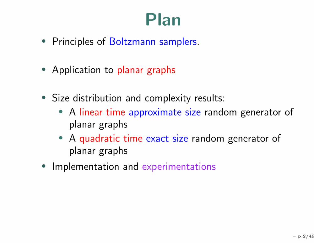
Plan• Principles of Boltzmann samplers.

• Application to planar graphs

• Size distribution and complexity results:• A linear time approximate size random generator of

planar graphs• A quadratic time exact size random generator of

planar graphs

• Implementation and experimentations

– p.2/49

The general framework ofBoltzmann samplers

– p.3/49

Idea of Boltzmann samplers

• Introduced by Duchon, Flajolet, Louchard and Schaeffer(2002)

• Relax the constraint of fixed size (cf recursive method)for random generation.

• The distribution is spread over all objects of the class.

• An object is drawn with probability proportional to theexponential of its size (cf statistical physics)

– p.4/49

Unlabelled sets• Let C be an unlabelled combinatorial class

(e.g. binary trees)Ordinary generating function:

C(x) =∑

γ∈C

x|γ| =∑

n≥0

cnxn,

where |γ| is the size of γ.

• Given x > 0 (x ≤ ρC) a fixed real value,a Boltzmann sampler ΓC(x) is a procedure that drawseach object γ of C with probability:

Pr(γ) = x|γ|

C(x)

– p.5/49

Finite sets

Let E = (γ1, . . . , γd) E(x) =∑d

i=1 x|γi|

ΓE(x)

γ1 γi γd

x|γi|

E(x)

. . .

. . .

. . .

x|γd|

E(x)x|γ1|

E(x) . . .

– p.6/49

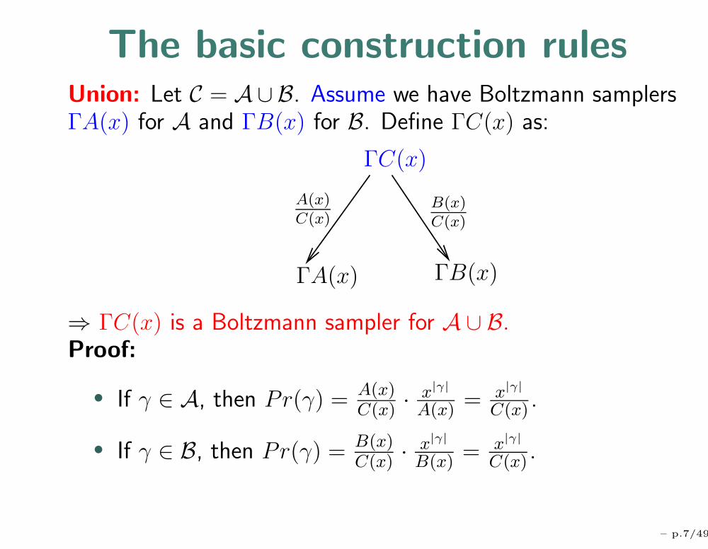
The basic construction rulesUnion: Let C = A∪B. Assume we have Boltzmann samplersΓA(x) for A and ΓB(x) for B. Define ΓC(x) as:

ΓC(x)

B(x)C(x)

A(x)C(x)

ΓA(x) ΓB(x)

⇒ ΓC(x) is a Boltzmann sampler for A ∪ B.Proof:

• If γ ∈ A, then Pr(γ) = A(x)C(x) ·

x|γ|

A(x) = x|γ|

C(x) .

• If γ ∈ B, then Pr(γ) = B(x)C(x) ·

x|γ|

B(x) = x|γ|

C(x) .

– p.7/49

The basic construction rulesProduct: Let C = A× B. Assume we have Boltzmannsamplers ΓA(x) for A and ΓB(x) for B. Define ΓC(x) as:

ΓC(x) : γ1 ← ΓA(x)

γ2 ← ΓB(x)

return (γ1, γ2)

⇒ ΓC(x) is a Boltzmann sampler for A ∪ B :Proof: an object γ = (γ1, γ2) has probability:

x|γ1|

A(x)

x|γ2|

B(x)=

x|γ1|+|γ2|

A(x) · B(x)=

x|γ|

C(x)

– p.8/49

Example: binary trees

orB B

B

Generating function

B(x) = x + B(x)2Boltzmann sampler

ΓB(x)

return leaf return

ΓB(x) ΓB(x)

– p.9/49

Result for unlabeled setsTheorem:

• A Boltzmann sampler can be assembled for an unlabeledclass specified with the constructions ∪, ×, Sequence.

• The complexity is linear in the size of the output object.

Construction Boltzmann sampler ΓC(x)

C = ∅ return ∅

C = • return •

C = A ∪ B Bern(

A(x)C(x)|B(x)C(x)

)

? ΓA(x)|ΓB(x)

C = A× B return (ΓA(x),ΓB(x))

C = Seq (A) k ← Geom (A(x))

return (ΓA(x), . . . ,ΓA(x)) { k calls}

– p.10/49

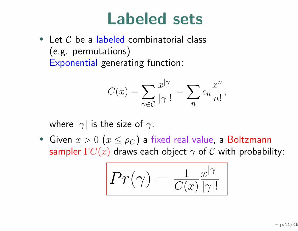
Labeled sets• Let C be a labeled combinatorial class

(e.g. permutations)Exponential generating function:

C(x) =∑

γ∈C

x|γ|

|γ|!=

∑

n

cnxn

n!,

where |γ| is the size of γ.

• Given x > 0 (x ≤ ρC) a fixed real value, a Boltzmannsampler ΓC(x) draws each object γ of C with probability:

Pr(γ) = 1C(x)

x|γ|

|γ|!

– p.11/49

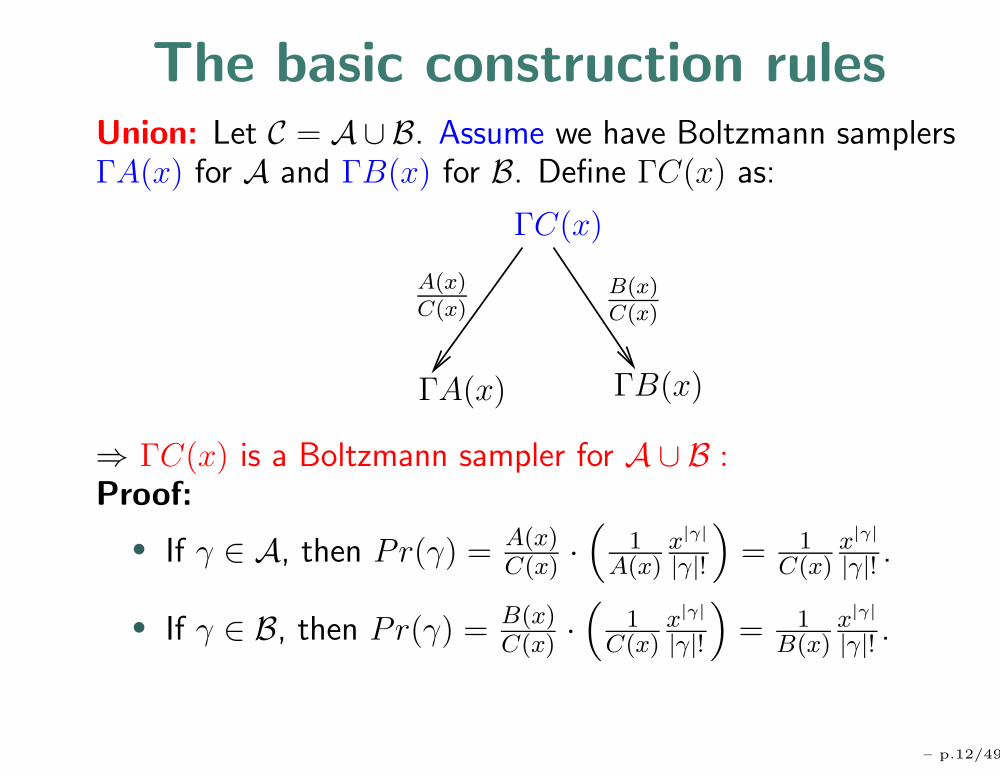
The basic construction rulesUnion: Let C = A∪B. Assume we have Boltzmann samplersΓA(x) for A and ΓB(x) for B. Define ΓC(x) as:

ΓC(x)

B(x)C(x)

A(x)C(x)

ΓA(x) ΓB(x)

⇒ ΓC(x) is a Boltzmann sampler for A ∪ B :Proof:

• If γ ∈ A, then Pr(γ) = A(x)C(x) ·

(1

A(x)x|γ|

|γ|!

)

= 1C(x)

x|γ|

|γ|! .

• If γ ∈ B, then Pr(γ) = B(x)C(x) ·

(1

C(x)x|γ|

|γ|!

)

= 1B(x)

x|γ|

|γ|! .

– p.12/49

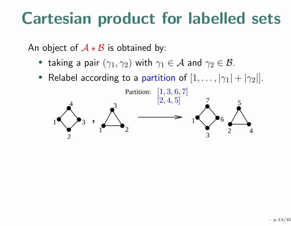
Cartesian product for labelled sets

An object of A ? B is obtained by:

• taking a pair (γ1, γ2) with γ1 ∈ A and γ2 ∈ B.

• Relabel according to a partition of [1, . . . , |γ1|+ |γ2|].

5

2 4

4

2

31

Partition:

3

1 21

7

6

3

,

[1, 3, 6, 7][2, 4, 5]

– p.13/49

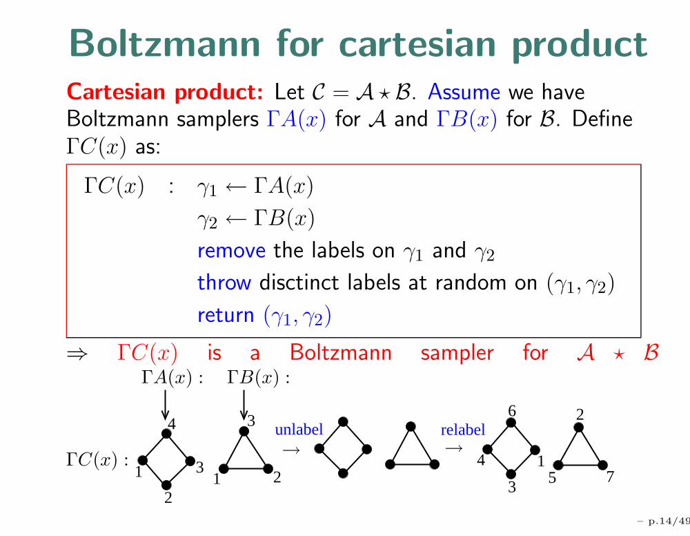
Boltzmann for cartesian productCartesian product: Let C = A ? B. Assume we haveBoltzmann samplers ΓA(x) for A and ΓB(x) for B. DefineΓC(x) as:

ΓC(x) : γ1 ← ΓA(x)

γ2 ← ΓB(x)

remove the labels on γ1 and γ2

throw disctinct labels at random on (γ1, γ2)

return (γ1, γ2)

⇒ ΓC(x) is a Boltzmann sampler for A ? B

1

4

2

3

3

1 21

3

4

26

75

relabelunlabel→ →

ΓB(x) :ΓA(x) :

ΓC(x) :

– p.14/49

Result for labeled sets

Theorem:

• A Boltzmann sampler can be assembled for a labeledclass specified with the constructions ∪, ×, Set.

• The complexity is linear in the size of the output object.

• The labels have just to be thrown at the end.

– p.15/49

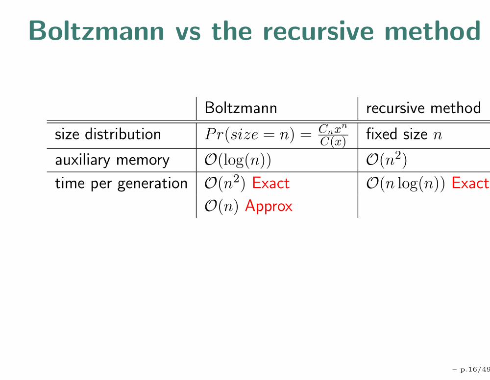
Boltzmann vs the recursive method

Boltzmann recursive method

size distribution Pr(size = n) = Cnxn

C(x) fixed size n

auxiliary memory O(log(n)) O(n2)

time per generation O(n2) Exact O(n log(n)) Exact

O(n) Approx

– p.16/49

Planar graphs and Boltzmannsamplers

– p.17/49

Labeled Planar graphs• A labelled graph with n vertices is a set of edges on the

labeled vertex-set V = [1, . . . , n].

• A graph is planar if it can be embedded in the plane.

3 4

52crossing

1

K is not planar5

• The embedding does not count (6= planar maps)

6

3

2

4

71 2

4

75

15

3

6

– p.18/49

Random generation of planar graphs

Existing algorithms:

• Markov chain (Denise, Vasconcellos, Welsh):simple algorithm but unknown convergence rate (mixingtime)

• Recursive method (Bodirsky, Gropl, Kang): Polynomialtime algorithm for uniform random generation of planargraphs with n vertices but large preprocessing time(many coefficients need to be stored).

– p.19/49

What new has to be done?To design a Boltzmann sampler for labeled planar graphs, wehave to do the following:

• A planar graph has labeled vertices and unlabeled edges:⇒ define the Boltzmann framework for the case of amixed class (two variables)

• Add the substitution (composition of G.f.) to theconstructions.

• Add rejection techniques to do derooting/rerootingoperations on the graphs

– p.20/49

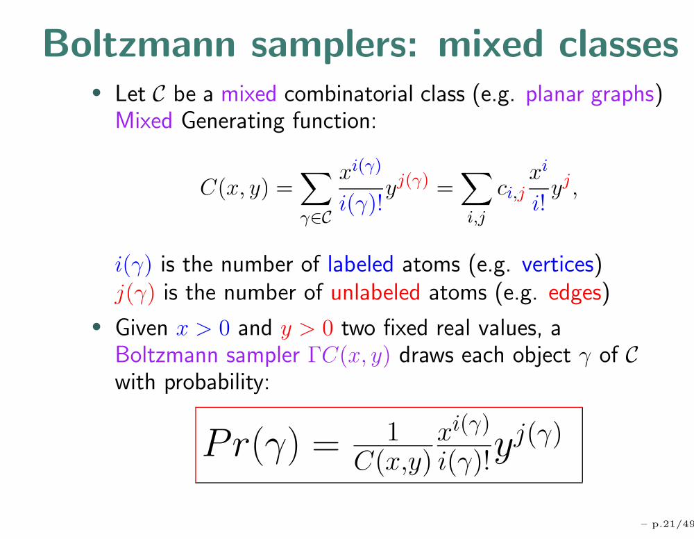
Boltzmann samplers: mixed classes• Let C be a mixed combinatorial class (e.g. planar graphs)

Mixed Generating function:

C(x, y) =∑

γ∈C

xi(γ)

i(γ)!yj(γ) =

∑

i,j

ci,jxi

i!yj ,

i(γ) is the number of labeled atoms (e.g. vertices)j(γ) is the number of unlabeled atoms (e.g. edges)

• Given x > 0 and y > 0 two fixed real values, aBoltzmann sampler ΓC(x, y) draws each object γ of Cwith probability:

Pr(γ) = 1C(x,y)

xi(γ)

i(γ)!yj(γ)

– p.21/49

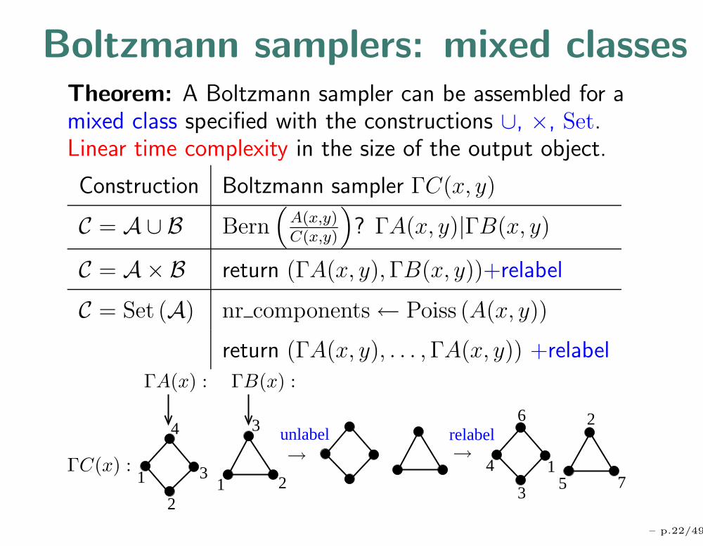
Boltzmann samplers: mixed classesTheorem: A Boltzmann sampler can be assembled for amixed class specified with the constructions ∪, ×, Set.Linear time complexity in the size of the output object.

Construction Boltzmann sampler ΓC(x, y)

C = A ∪ B Bern(

A(x,y)C(x,y)

)

? ΓA(x, y)|ΓB(x, y)

C = A× B return (ΓA(x, y),ΓB(x, y))+relabel

C = Set (A) nr components← Poiss (A(x, y))

return (ΓA(x, y), . . . ,ΓA(x, y)) +relabel

1

4

2

3

3

1 21

3

4

26

75

relabelunlabel→ →

ΓB(x) :ΓA(x) :

ΓC(x) :

– p.22/49

Boltzmann samplers: substitution• The class C = A ◦ B consists of objects of A where each

atom is replaced by an object of BG.f.: C(x) = A(B(x))

• Boltzmann sampler:

ΓC(x) γ ← ΓA (B(x))

replace each atom of γ by ΓB(x)

• very simple and no need of Bernoulli-choices (unlike therecursive method)

1

2

4

3

1

23

1

2

3

1

2

– p.23/49

Conception of a Boltzmannsampler for planar graphs

– p.24/49

Overview of the method

• Decomposition according to successive levels ofconnectivity:Planar graph → Connected → 2-connected →3-connected

• Combinatorial bijection (Fusy, Poulalhon, Schaeffer)3-connected graphs ↔ binary trees

– p.25/49

Planar graphs

Disconnected

Connected

2-connected

3-connected

– p.26/49

Planar graphs → connected p. g.• Let G be the set of planar graphs

• Let C be the set of connected planar graphs

• A planar graph is decomposed into connectedcomponents⇒ G = Set(C) G(x) = exp(C(x))

ΓG(x, y) : k ← Poiss(C(x, y))

return (ΓC(x, y), . . . ,ΓC(x, y)) { k calls}

– p.27/49

Connected → 2-connectedDecomposition by vertex-substitution:A pointed connected planar graph is a set of pointed2-connected planar graphs where each non pointed vertex issubstituted by a pointed connected planar graph.

⇒ C•(x, y) = x exp(B′(C•(x, y), y))

– p.28/49

Connected → 2-connected

C•(x) = x exp(B′(C•(x)))

ΓC•(x): 1) k ← Poiss(λ := B′(C•(x)) exp(. . .)

2) γ ← (ΓB•(C•(x)), . . . ,ΓB•(C•(x)))︸ ︷︷ ︸

k times

exp(B′(. . .))

3) merge the k marked vertices of γ

4) for each non-marked vertex v of γ

substitute v by γv ← ΓC•(x) exp(B′(C•(x)))

5) return γ

⇒ Finding ΓC• reduces to finding ΓB•

– p.29/49

2-connected → 3-connected• Decomposition by edge-substitution.

• B(x, y) series of 2-connected planar graphs.

• G3(x, y) series of 3-connected planar graphs

∂B∂y (x, y) ≈ ∂G3

∂y

(

x, ∂B∂y (x, y)

)

⇒ Finding Γ∂B∂y reduces to finding Γ∂G3

∂y

– p.30/49

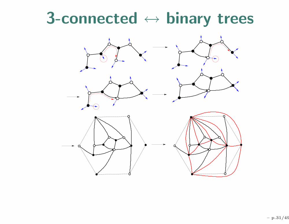
3-connected ↔ binary trees

– p.31/49

3-connected ↔ binary treesFusy, Poulalhon, Schaeffer 2005:Binary trees are in bijection with edge-pointed 3-connectedplanar graphs.

i j i+3 verticesi+j+4 edges

– p.32/49

Boltzmann sampler for planar graphs

edge−pointed3−connected graph

edge−pointed2−connected graph2−connected graph

vertex−pointed

edge−substitution

rejection

bijection

rejectionconnected graph

connected components

vertex−substitution

vertex−pointedconnected graph

binary tree Γ∂G3

∂y(x, y)

Γ∂B∂y

(x, y)

ΓC(x, y)

ΓT (x, y)

Γ∂C∂x

(x, y)

Γ∂B∂x

(x, y)

planar graph ΓG(x, y)

– p.33/49

Rejection for Boltzmann samplers• Let B be a combinatorial class for which we have a

Boltzmann sampler.

• Let A ⊂ B be a combinatorial class for which we want aBoltzmann sampler.

ΓA(x) : γ ← ΓB(x)

if γ ∈ A return γ else restart

Then ΓA(x) is a Boltzmann sampler for A.

The acceptance probability at each try is

Paccept =∑

γ∈A

x|γ|

B(x)=

A(x)

B(x)

– p.34/49

Applications

1

3

4

5

2

6

1

3

42

6 5

choose smallestneighbour

Γ∂B∂x (x, y) from Γ∂B

∂y (x, y)

⇒ Γ∂B∂x (x, y) : γ ← Γ∂B

∂y (x, y)if the end of the root-edge is the smallest neighbour

•

of the origin of the root-edge, return γelse restart

B• is a subset of B→ :

else restart

ΓC(x, y) from ΓC•(x, y)

C is a subset of C• :

⇒ ΓC(x, y) : γ ← ΓC•(x, y)if the pointed vertex has label 1, return γ

•

1mark 1

2

3

4 1

2

3

4

– p.35/49

Derivation of an efficientsampler

– p.36/49

How to achieve a target size n?

• We have a Boltzmann sampler ΓG(x, 1) for planargraphs

• We want to achieve a target-size n

• We have to choose x = xn so that ΓG(xn) producesgraphs of size n with good probability.

• Natural choice: xn such that E(size(ΓG(xn))) = n

• The function x→ E(size(ΓG(x))) is increasing⇒ xn has to converge to ρG (dom. sing.) when n→∞.

– p.37/49

Size distributionProblem: Even at the singularity ρG, the expected size ofΓG(ρG) remains bounded:

Pr(size = n) =Gnρn

GG(x) ∼

cn7/2

(Gimenez, Noy 2005)proba

size

c/n7/2

Size distribution of the output of ΓG(ρG)

– p.38/49

Improve the size distributionSolution: point the graphs 3 timesEffect: multiply coefficient Gn by n3.

proba

size

proba

size

1/n7/2

n

1/n

Output of ΓG(ρG) Output of ΓG•••`

ρG(1 − 1

2n)´

– p.39/49

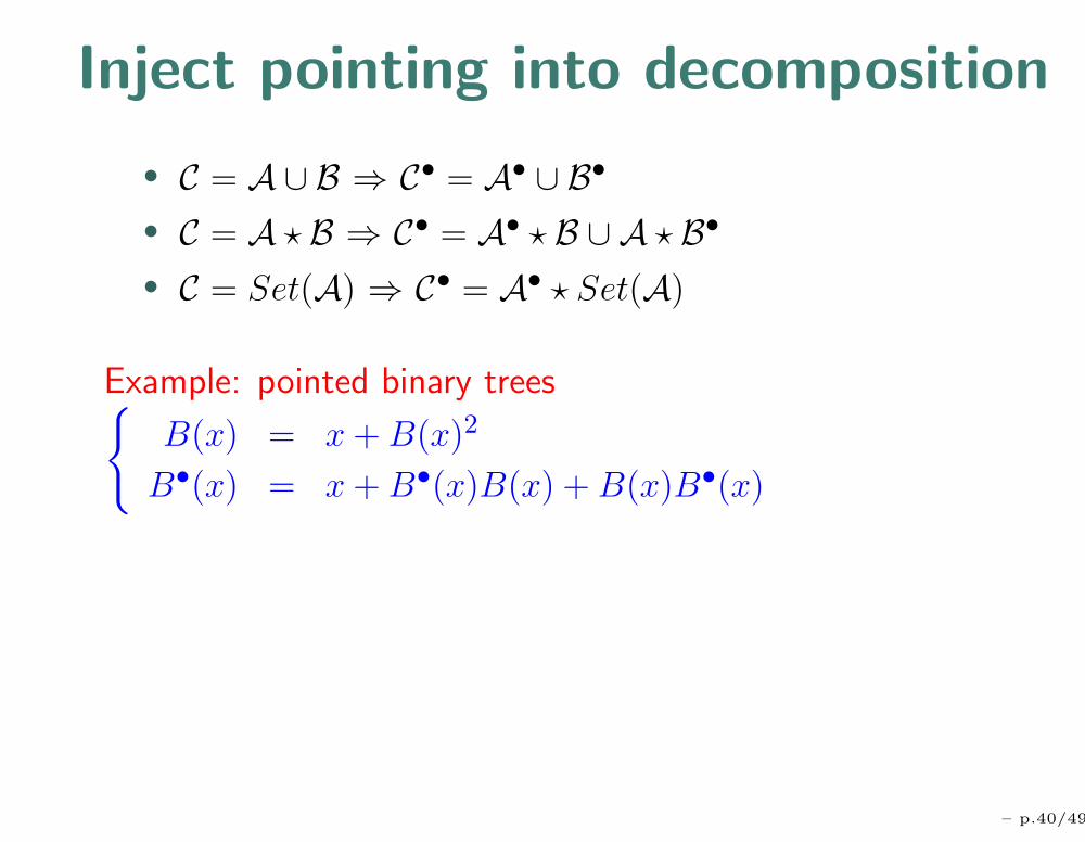
Inject pointing into decomposition

• C = A ∪ B ⇒ C• = A• ∪ B•

• C = A ? B ⇒ C• = A• ? B ∪ A ? B•

• C = Set(A) ⇒ C• = A• ? Set(A)

Example: pointed binary trees{

B(x) = x + B(x)2

B•(x) = x + B•(x)B(x) + B(x)B•(x)

– p.40/49

Main resultsLet n be a target size and ε be a (relative) size-tolerance.

Take ΓG•••(xn) at xn = ρG

(1− 1

2n

).

Theorem The generator ΓG•••(xn) produces planar graphs:

• with size in [n(1− ε), n(1 + ε)] in linear time. APPROX

• with size n in quadratic time. EXACT

Aux. memory Prep. time Time per generation

Markov O(log n) O(1) unknown {exact size}

Recursive O(n5 log n) O (n7) O(n3) {exact size}

Boltzmann O((log n)k) O((log n)k) O(n2) {exact size}

O(n) {approx. size}

– p.41/49

Changing the ratio edges-vertices• Let y > 0 be a fixed real value.

• For n 6= 1, let xn be such thatE (size(ΓG•••(xn, y))) = n

Result: There exists a constant µ(y) ∈ (1, 3) such that theratio edges-vertices of the output of ΓG•••(xn, y) is almostsurely equal to µ(y) when n→ +∞.

1.2

1.4

1.6

1.8

2

2.2

2.4

2.6

2.8

mu

2 4 6 8 10

y

– p.42/49

Grammar for complexity calculationLet C be a class and x > 0 a real valueDefine ΛC(x) as the average number of operations of ΓC(x).

• Union:

ΓC(x) : Bern(

A(x)C(x) |

B(x)C(x)

)

? : ΓA(x)|ΓB(x)

ΛC(x) = A(x)C(x) · ΛA(x) + B(x)

C(x) · ΛB(x)

• Product:ΓC(x) : (ΓA(x),ΓB(x)).

ΛC(x) = ΛA(x) + ΛB(x)

• Set:ΓC(x) : Poiss (A(x))⇒ ΓA(x)

ΛC(x) = E (Poiss (A(x))) · ΛA(x) = A(x) · ΛA(x)

– p.43/49

Grammar for complexity calculationLet C be a class and x > 0 a real valueDefine ΛC(x) as the average number of operations of ΓC(x).Define ΣC(x) as the average size of ΓC(x).

• SubstitutionΓC(x) : replace each atom of ΓA(B(x)) by ΓB(x)

ΛC(x) = ΛA(B(x)) + ΣA(B(x)) · ΛB(x)

• RejectionA ⊂ BΓA(x) : do γ ← ΓB(x) until γ ∈ A

ΛA(x) = B(x)A(x) · ΛB(x)

– p.44/49

Complexity results

• For all instances of rejection A ⊂ B, the

acceptance-probability A(xn)B(xn) is bounded away from 0

when n goes to ∞.

• The grammar for calculations implies the followingresult:Theorem: For n ≥ 1, let xn be such that the expectedsize of ΓG•••(xn) is n. Then:

ΛG•••(xn) = O(n).

– p.45/49

Implementation andexperimental results

– p.46/49

Overview of the implementation

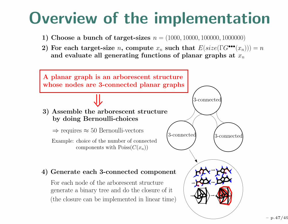
For each node of the arborescent structuregenerate a binary tree and do the closure of it

3-connected

3-connected 3-connected

1) Choose a bunch of target-sizes n = (1000, 10000, 100000, 1000000)

by doing Bernoulli-choices

Example: choice of the number of connectedcomponents with Poiss(C(xn))

⇒ requires ≈ 50 Bernoulli-vectors

(the closure can be implemented in linear time)

2) For each target-size n, compute xn such that E(size(ΓG•••(xn))) = n

3) Assemble the arborescent structure

and evaluate all generating functions of planar graphs at xn

A planar graph is an arborescent structurewhose nodes are 3-connected planar graphs

4) Generate each 3-connected component

– p.47/49

Experimental resultsLet Xn be the number of edges of a random planar graph onn vertices.Theorem: (Gimenez, Noy)There exists a constant µ ≈ 2.2132, such that

Xn

n→ µ almost surely when n→∞

2.18

2.2

2.22

2.24

ratio edges-vertices

0 20 40 60 80

Tries in chronological order

– p.48/49

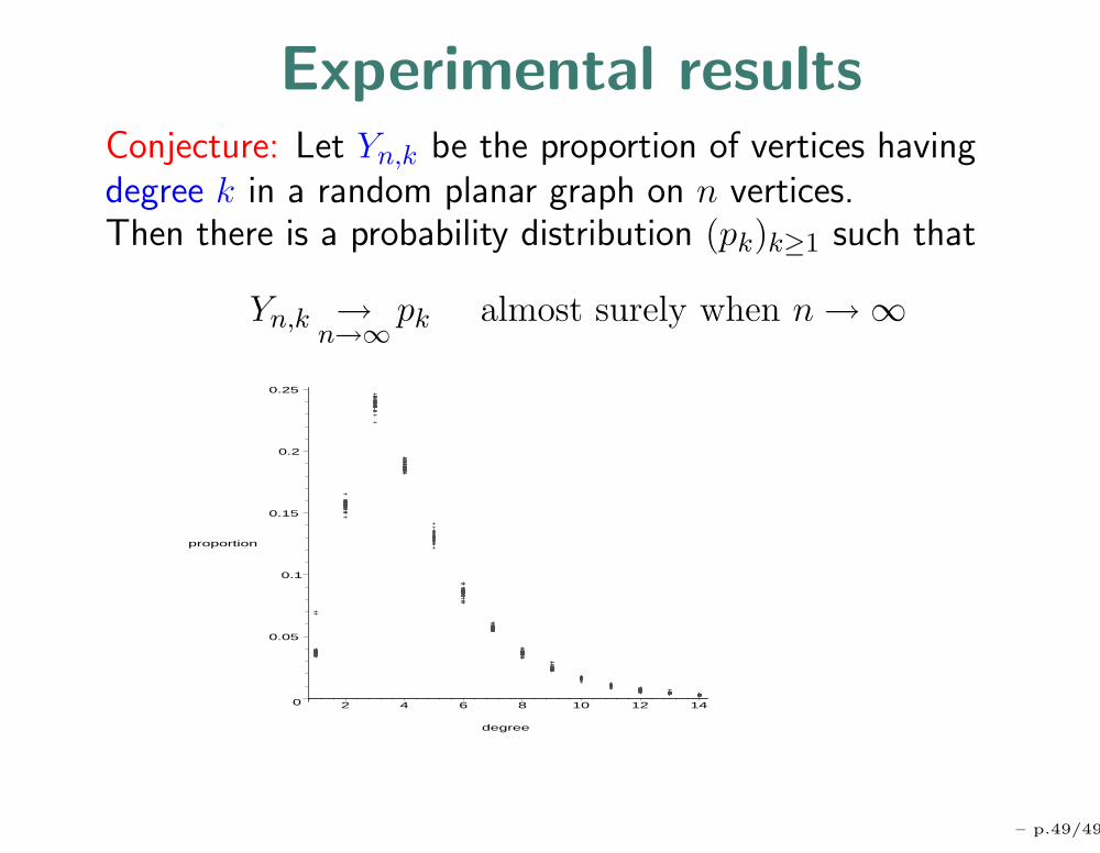
Experimental resultsConjecture: Let Yn,k be the proportion of vertices havingdegree k in a random planar graph on n vertices.Then there is a probability distribution (pk)k≥1 such that

Yn,k →n→∞

pk almost surely when n→∞

0

0.05

0.1

0.15

0.2

0.25

proportion

2 4 6 8 10 12 14

degree

– p.49/49