(a ) LOC1 LOC2 LOC3 LOC4 Towards an IFC-Modelica … · 1KU Leuven, Department of Civil Engineering, Building Physics Section, ... or level of detail, ... A first part of this paper

Proceedings of the 15th IBPSA ConferenceSan Francisco, CA, USA, Aug. 7-9, 2017

2257https://doi.org/10.26868/25222708.2017.621

Towards an IFC-Modelica tool facilitating model complexity selection for building energy

simulation

Glenn Reynders1,2, Ando Andriamamonjy1,3, Ralf Klein3, Dirk Saelens1,2

1KU Leuven, Department of Civil Engineering, Building Physics Section,

Kasteelpark Arenberg 40 – box 2447, BE-3001 Heverlee, Belgium 2EnergyVille, Thor Park 8310, BE-3600 Genk, Belgium

3 KU Leuven, Technology Cluster Construction, Technology Campus Ghent, Gebroeders De

Smetstraat 1, BE-9000 Ghent, Belgium

Abstract

This paper presents a novel tool chain that enables a direct

coupling between building information models (BIM) and

building energy simulation (BES) models developed in

Modelica. In contrast to similar tools found in literature,

the novel tool chain is a Python implementation that

provides a direct coupling between BIM and Modelica

and focuses on the thermal modelling of building

envelopes.

The main innovation in this tool chain is that it provides

increased user flexibility by facilitating a BES model

generation with different levels of complexity, which is

demonstrated on a real-life experiment. In this case study,

significant savings in simulation time were obtained

without significantly affecting the model accuracy in

terms of predicting energy use and load-duration curves,

if the aggregation of zones reflects the control strategy for

space heating.

Introduction

BIM is regarded as a data source for building energy

simulation which is currently becoming an increasingly

important and reliable BES input to relieve modellers

from the time consuming and error prone data gathering

process. In this context and in a non-exhaustive way,

(Dimitriou et al., 2016; Kim et al., 2016) have

investigated the translation of BIM formats such as

Industry Foundation Class (IFC) (EN ISO 16739:2016)

and Green Building xml (GBXML) into the widely used

building simulation engine EnergyPlus (Crawley et al.,

2001).

At the same time, due to the limitations of these traditional

simulation engines (EnergyPlus, DOE-2,…) (Wetter,

2009), the multi-disciplinary and flexible modelling

language Modelica has gained recent attention. (Jeong et

al., 2014, 2016) use a proprietary software API as an

interface to generate a building simulation Modelica

model. (Andriamamonjy et al., 2016; Thorade et al., 2015;

Remmen et al., 2015) propose an open framework capable

of translating the open-BIM format IFC into a building

energy simulation Modelica model.

A common point amid these BIM based methodologies is

the focus towards detailed BES models, whereby a one-

to-one mapping of the components between BIM and

BES is carried out. Such detailed BES models are utilized

when sufficient data is available and when accuracy

prevails before simulation speed. However, this

modelling approach may result in high computational

costs for complex and large buildings. Moreover, not all

relevant input data for such detailed models may in

practice (e.g. during the early design phase) be available.

Also, a less complex model would be adequate depending

on the specific application (e.g. MPC or FDD during

operational phase).

Currently, switching from one type of BES model to

another is a time consuming task involving several tools

and programs. Hence, an intelligent matching of the

complexity, or level of detail, of the BES model to the

specific application or phase in the building design

process is difficult to achieve in practice.

To simplify this process, this paper proposes an open

PYTHON tool chain leveraging IFC features to

automatically generate a set of building geometry models

implemented in Modelica with different levels of

complexity. The focus of this tool chain is currently

oriented towards thermal simulations and only considers

the thermal envelope. To our knowledge, such a tool or

platform capable of generating building energy

Information update

Topology generation

Mapping process

LOC1

1 LOC IDEAS model

Topology generation

Mapping process

LOC1

4 LOC IDEAS model

LOC2 LOC3 LOC4

Information update

Level of complexity generation

IFC2X3 IFC4

IFC conform

(b)

(a)

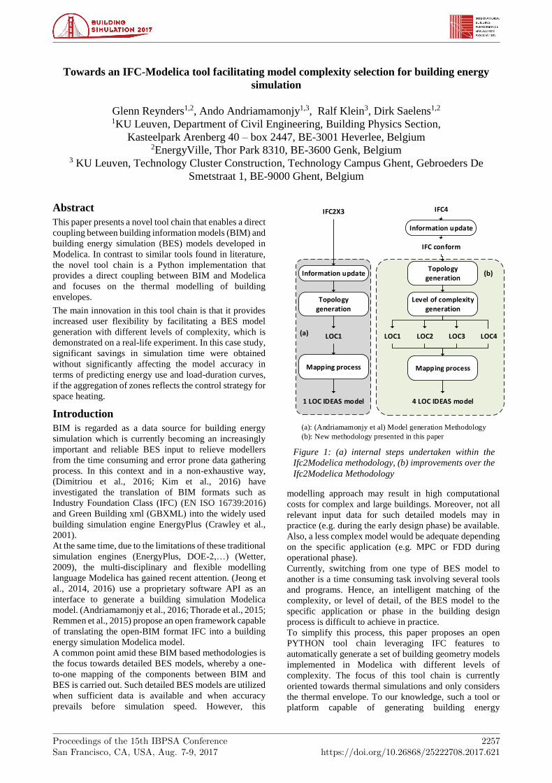
(a): (Andriamamonjy et al) Model generation Methodology

(b): New methodology presented in this paper

Figure 1: (a) internal steps undertaken within the

Ifc2Modelica methodology, (b) improvements over the

Ifc2Modelica Methodology


2258

simulation models with several levels of complexity from

a unique BIM data source is still missing.

The new tool chain is a continuation of the work

undertaken by Andriamamonjy et al. (2016). In contrast

to many existing IFC into Modelica methodologies, the

direct translation of IFC objects into Modelica

components is performed without the use of middleware,

using a compact, easy to use PYTHON framework. The

new tool chain presented in this paper appends a set of

improvements enabling the generation of four levels of

detail ranging from a highly detailed mapping of IFC

entities into Modelica components to a simplified model

aggregating the spaces on each floor. This paper uses the

Integrated District Energy Assessment Simulations

library (IDEAS) (Baetens et al., 2015) to translate a BIM

model into four Models with different levels of

complexity.

A first part of this paper details the improvements applied

to the methodology of (Andriamamonjy et al., 2016) and

the implementation of the level of complexities in the

methodology. A second part demonstrates the impact of

the different levels of complexity in terms of simulation

speed and accuracy considering total energy use,

temperature profiles and load-duration curves. As a

demonstration case, the tool chain is applied on the

TwinHouse test building located in Holzkirchen,

Germany (Strachan et al., 2015). Although the

Holzkirchen test facility is a relatively small

demonstration case, similar trends can be expected for a

larger and more complex building.

Methodology

This section presents the general improvements

introduced over the Andriamamonjy et al. (2016)

methodology (referred as Ifc2Modelica), and shows how

the model generation process has been modified to enable

the integration of different levels of complexity.

Figure 1 presents the comparison between Ifc2Modelica

and the new tool chain presented in this work (referred as

Ifc2Modelica v0.2). Figure 1.a presents the Ifc2Modelica

methodology and the four steps required to generate a

detailed IDEAS Modelica model which are respectively:

‘IFC parsing layer’, ‘information update’, ‘the topology

generation’, and ‘the mapping process.’ The

improvements introduced to each of these steps are

presented in Figure 1.b and will be explained throughout

this section.

General improvements to Ifc2Modelica

One of the strengths of Ifc2Modelica is the use of IFC as

the main data model. IFC is directly translated into

Modelica avoiding the use of an intermediate tool/data

model which might fall outside of the energy modeller

expertise domain. Besides, Ifc2Modelica is a fully

compact PYTHON framework capable of generating a

Modelica model including a graphical layout. The

graphical layout enables the representation of Modelica

components (via the “annotation” statement) within the

Modelica simulation engine (e.g. Dymola,

OpenModelica) which facilitates a subsequent

modification of the generated energy simulation model.

As an important drawback, Ifc2Modelica relied on the

previous IFC version IFC2X3 with the standard

coordination view 2.0 Model View Definition (MVD)

(Hafele et al., 2013) (see Figure 1). IFC2X3 does not have

all the appropriate entities and relationships to fulfil the

needs of building energy simulation. Hence, tools,

middleware or embedded algorithm are used to adapt

IFC2X3 for energy simulation. To overcome this issue,

this new tool chain (referred as Ifc2Modelica v0.2) uses

IFC4. IFC4 is a semantic rich format where improvements

have been introduced with regard to energy simulation

requirements (Liebich, 2013).

However, BIM software certification towards IFC4 is still

lagging behind. Although some BIM software provide an

IFC4 export option, limitations are noted which cause an

information loss during the IFC export from the BIM

software. This requires that the IFC files generated from

any BIM software are checked to verify whether the

information required for energy simulation is available.

In the case where information is missing, Ifc2Modelica

v0.2 gives the modeller the ability to update the

information within the IFC file. Within the “information

update” step (see Figure 1), the BIM model is validated

against a subset of IFC schema defining the requirements

for energy simulation (a Model View Definition, MVD)

(Hietanen, 2008). In this study, an MVD has been

implemented similar to the one presented by Pinheiro et

Al (Pinheiro et al., 2016). The buildingSMART tool

IfcDoc v11.2 (Liebich et al., 2017) was used for the MVD

creation. If a discrepancy is identified between the content

of the IFC file and the requirements of the MVD, a list

(spreadsheet file) of the missing properties, entities and

relationships is generated by Ifc2Modelica. The modeller

then completes the information within the spreadsheet.

Subsequently the spreadsheet is used as an input to

Ifc2Modelica v0.2 to obtain a MVD-conform IFC file.

Ifc2Modelica v0.2 updates the missing information

directly into the IFC file by using a PYTHON routine

(‘information update’, Figure 1) based on the PYTHON

library IfcOpenShell (Krijnen et al., 2015).

Finally, the ability to generate several levels of model

complexity is the main improvement introduced by the

tool chain. Each level of complexity is targeted to suit the

needs of a specific BES application either in terms of

accuracy, simulation speed or data availability.

Translation into Modelica model

In order to explain the fundamental concepts of the

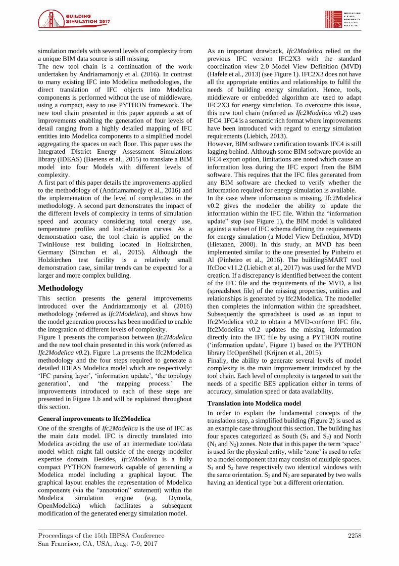
translation step, a simplified building (Figure 2) is used as

an example case throughout this section. The building has

four spaces categorized as South (S1 and S2) and North

(N1 and N2) zones. Note that in this paper the term ‘space’

is used for the physical entity, while ‘zone’ is used to refer

to a model component that may consist of multiple spaces.

S1 and S2 have respectively two identical windows with

the same orientation. S2 and N2 are separated by two walls

having an identical type but a different orientation.


2259

For the translation of the BIM to IDEAS, this new tool

chain relies on a similar methodology as Ifc2Modelica but

introduces a set of IFC based algorithms enabling to

generate several levels of model complexity which will be

further explained in this section.

The model generation process has 3 main steps (see

Figure 1):

Topology generation

Level of complexity generation

Mapping process

Topology generation

The topology generation parses the IFC file and creates a

PYTHON class image of each IFC entity in the file. The

topology generation process adapts these classes to be

compatible with the IDEAS library and to enable a

seamless mapping between the classes and IDEAS

components.

Within IDEAS, external walls, internal walls, roofs,

windows, floors on ground and zones are represented by

individual Modelica components. Thus, a building

simulation model in IDEAS is composed by a set of

instances of those components interconnected by

Modelica connect statements. For instance, an IDEAS

“outside wall component” (Jorissen et al., 2017) has a

connector (propsBus_a) through which the wall

"exchanges" heat flow with a space.

The topology generation process identifies the classes

representing a building geometry element (wall, roof…).

These classes will be referred to as “component classes”

and will be mapped into IDEAS components. Port

concepts similar to the Modelica connectors are attributed

to each component class. In addition, the topology

generation process identifies the classes that could be

used to represent the flow exchange between the

component classes. These classes, referred to as

“connection classes”, will be mapped into Modelica

connections.

Component class. IfcSpace entities and subtypes of

IfcBuildingElement entities (IfcWallStandardCase,

IfcRoof, IfcWindow, IfcSlab...) are categorized as a

component class. However, some specific cases have to

be taken into account. Due to the chosen architectural

description of building elements in BIM, the construction

entities (e.g. IfcWallStandarCase) can span several spaces

(e.g. wall1 in Figure 2); which is not compatible with the

one dimensional heat transfer adopted in common

building energy simulation tools such as IDEAS. To

address the issue, Bazjanac et al (Bazjanac, 2010)

proposed the space boundary concept, which represents

the building elements with respect to spaces. The space

boundary concept was not included or not correctly

represented in the early version of the IFC standard (2X)

which led to the development of tools capable of

generating such concepts (Ladenhauf et al., 2016; Lilis et

al., 2016; Rose & Bazjanac, 2013). Nonetheless, major

improvements have been brought to the latest release of

IFC (IFC4) where a space boundary concept has been

integrated (Liebich, 2013). As the current study is based

on IFC4, the space boundary concept defined in IFC4 is

used to split the construction entities spanning several

spaces into several component classes (e.g. wall 1 will be

split into two component classes: Wall 1-1 and Wall 1-2).

Rose and Bazjanac (2013) proposes a comprehensive

algorithm to generate space boundary.

To represent the concept of a “port” similar to those of the

Modelica components, a set of additional parameters

(ports: "heat port", "fluid port" and "signal port") are

attributed to the component classes based on the type of

flow that the class (or the IFC entity it represents) can

"exchange" with its surrounding. For instance, an internal

wall exchanges heat flow from one space to another, thus

two "heat ports" are attributed to a component class

representing an internal wall (IfcWallStandardCase). In

contrast, a space can exchange heat and fluid with its

surrounding. Thus a heat port is attributed to a component

class representing a space (IfcSpace) alongside with two

"fluid ports" with opposite flow directions. As an IDEAS

component has several Modelica connectors, the port

attribution enables to precisely define the Modelica

connector through which the connection will be

implemented during the mapping.

Connection class. A connection class defines the pair of

component classes that need to be interconnected

alongside with the type of corresponding ports ("heat

port", "fluid port" and "signal port") through which the

two component classes have to be connected.

For example, a connection class is established between a

component class representing a subtype of

IfcBuildingElement and a component class representing

an IfcSpace that are linked through the space boundary

N1

S1

Wall 1

Sb: Space boundary

Sb1N2

Sb2N2Sb1N1

Wall 1-1

(internal)

Wall 1-2

(internal)

Wall 2

Wall 2-1

(external)

North space

South space

N2

S2

Win

Sb2N1

Figure 2 : Simple example building used to

demonstrate the concepts of the new tool chain


2260

concept (Liebich & Chipman, 2015). The connection is

established through the “heat port” of both component

classes.

The result of the topology generation step is a detailed

building topology (e.g. Figure 3, LOC1), where each

building element is represented by a component class. The

obtained topology corresponds to a one-on-one mapping

from IFC entities into Modelica components referred to

as level of complexity one (LOC1) (see Figure 3).

LOC1 would be suitable when a high level of data is

available and model accuracy prevails before simulation

time. For instance, during the building’s final design

phase, it could be used to accurately estimate the yearly

energy consumption, analyse thermal comfort on the level

of individual spaces or develop and optimize control

strategies for the building management system. However,

when computation time becomes critical, especially when

the complexity and size of the building increases, it may

not always be suitable to use such a detailed model.

Table 1 Overview of implemented levels of complexity in Ifc2Modelica v0.2

Level Of

Complexity

Definitions Aim Prospective usage during design

phase

LOC 1 One to one mapping of

IFC entities into

Modelica components.

Detailed Model with high accuracy Assessment of the final building

design or the effect of the renovation

strategy

LOC 2 LOC 1 + Merge

entities having the

same type, azimuth

and characteristics.

Similar accuracy than LOC1 with an

expected lower simulation time

Throughout the iterative design

process until the final design is

reached.

LOC 3 LOC 2 + Merge the

spaces belonging to an

identical zone.

Decrease LOC2 simulation time by

merging the spaces having similar

characteristics (zone)

Zoning process during HVAC

design. (could be used for Model

Predictive Control (MPC) or Fault

Detection and Diagnosis (FDD).)

LOC 4 LOC 3 + Merge the

spaces on the same

floor.

Decrease further the simulation time

by considering only the external

building shell

Focus on the external shape of the

building.

N1

(IfcSpace)

S1

N2

S2

N

S

LOC1LOC2 LOC3

LOC4

(1) Entities with identical type and

azimuth that have to be merged

(2) Entity categorized as partition

1

12

w D

wi

Wall

Window

Door

wi

D

w

Win2Win1

Wall 1-1

(internal)

Wall 1-2

(internal)

Wall 2-1

(external)

IfcWallIfcWindow

Mapping

Simplification path:

LOC 1->2->3->4

Figure 3: Mapping process and Levels of complexity of the example case


2261

The Level of complexity generation

The detailed models (LOC1) generated by the topology

generation might not cause high computational effort for

simple buildings, such as residential dwellings.

Nonetheless, the size of the simulation model may

increase drastically for large apartment blocks or office

buildings. To be able to easily adapt the model size and

hence limit the computation time, the tool chain provides

three IFC based algorithms enabling the generation of

three additional levels of complexity. Thereby the current

tool implementation only focusses on the thermal

representation of the building envelope in building energy

simulations. These algorithms have the following

features: (the IFC relationship or concepts used in this

section can be found in the IFC4 documentation (Liebich

& Chipman, 2015))

■ Entities having the same type (Object Typing concept),

the same azimuth (for external construction) and

bounding the same space are merged into a unique

component class. For instance, in the example case

(Figure 3) the entities framed in blue in the LOC1 are

merged into a single entity in the second level of

complexity (LOC2). Similar to LOC1, LOC2 requires a

high level of data but is assumed to have a lower

simulation time as less components than in LOC1 are

generated. The latter will have a significant impact when

a high number of repetitive building elements, such as

windows or columns, are linked to a zone.

■ Component classes representing spaces, belonging to

the same zone (e.g. North zone and south zone) through

the zone assignment concept, are merged. The properties

(e.g. volume) of the final space sub-entity is the

aggregation of the constituting space entities properties

(e.g. VN=VN1+VN2). Common constructions (e.g. framed

in green in Figure 3, LOC2) between the spaces are

categorized as partition construction. The boundary

constructions are the aggregation of the boundaries of the

constituting spaces (e.g. aggregation of the entities frames

in red in LOC2). This simplification constitutes the Level

of Complexity 3 (LOC3). LOC3 is suitable to assess the

zoning effect during the HVAC design enabling to

identify the optimal partition of the building.

■ Spaces belonging to the same floor through the Spatial

Decomposition concept are merged. This will be referred

as the Level of Complexity 4 (LOC4) (Figure 3) which is

assumed to have a lower simulation time and would be

suitable to analyse several preliminary building designs

focusing mainly on the external shape.

Mapping process

The mapping process translates the topology, regardless

of the level of complexity, into a graphically represented

Modelica model. It instantiates and populates a Modelica

component for each component class contained in the

previously generated topology.

Prior to the mapping, each component class must have a

corresponding Modelica component known beforehand.

This information is stored in a template library which

contains a set of component templates, each of them

describing a specific Modelica component corresponding

to an IFC entity.

A component template contains the type (and the subtype)

of the IFC entity compatible with the Modelica

component. It contains also the component path, the list

of parameters required for the component instantiation

and the port description. Table 2 presents the template of

the IDEAS zone component. The port description

provides the correspondence between the port attributed

to a component class and the Modelica component

connector. For instance, in Table 2, the “zone.propsBus”

connector corresponds to the “heat port” of a component

class representing a space entity. This information is

deduced from the IDEAS components documentation

(Jorissen et al., 2017).

Additionally the template contains the Modelica

annotation which enables to graphically represent the

component in the Modelica environment.

To construct the Modelica model, the mapping process

has five main steps:

1) A code routine identifies the corresponding Modelica

component for each component class in the topology. For

example, for a component class representing a space

entity (IfcSpace), the component template representing its

Modelica component, is presented in Table 2.

2) Subsequently, the ports of the component class and the

component template are compared. For instance, as

described in the topology generation, one “heat port” and

two “fluid port” were attributed to any component class

representing an IfcSpace entity.

3) The code routine then requests the value of the

parameters between delimiters (‘#’) and inserts them

within the component path to instantiate the component

(e.g.

“IDEAS.Buildings.Components.Zone(nSurf=5,V=150,h

Zone=2.7, A=55, n50=2)”)

4) Next, the Modelica connections between the

components are established. The information contained in

the connection class is used to connect the corresponding

components through their connectors.

5) Finally, the model is represented within the graphical

model layout, using the Dymola annotations.

Table 2 IDEAS zone component template

Zone

Type IfcSpace

Subtype N/A

component path IDEAS.Buildings.Components.

Zone

Port Description {port_a, port_b, propsBus}

{fluid port (in), fluid port (out),

heat port}

List of parameters nSurf=f(#SpaceBoundary#)

V=#GrossVolume#

hZone=#Height#

A=#GrossFloorArea#

N50=#n50#

Annotation annotation

(Placement(transformation(ext

ent={{x0,y0},{xw,yW}})))


2262

Application

To demonstrate the Ifc2Modelica v0.2 tool chain and to

analyse the impact of the different aggregation steps on

the model accuracy and the simulation time, the new tool

chain is applied on a real-life case study, i.e. the

TwinHouse model validation experiment. This

experiment was carried out in the framework of IEA EBC

Annex 58 and consists of a whole building dynamic

heating experiment. Although the added value of

Ifc2Modelica v0.2 is expected to increase for larger,

repetitive buildings (e.g. traditional office buildings,

apartment blocks), the TwinHouse case is chosen as it is

a well-documented test case which was already used to

verify the accuracy of the IDEAS building library

(Reynders, 2015).

The experiment, as described in (Strachan et al., 2016), is

carried out in one of the TwinHouse buildings at the

Fraunhofer institute in Holzkirchen (Germany). The

building consists of 9 zones of which, 7 zones (Figure 4)

are subject to the experiment while the attic (zone 8) and

the basement (zone 9) are treated as boundary conditions.

The 4 South oriented zones (1. Living, 2. Bedroom 1, 3.

Bathroom, 4. Corridor) are equipped with a mechanical

ventilation system with supply in the ‘Living’ and exhaust

in both ‘Bedroom 1’ and ‘Bathroom’. To facilitate air

circulation, the doors between the zones were fully open.

The doors to the 3 Northern zones are sealed and no

mechanical ventilation is used in these zones. In all rooms

except the corridor, direct electric heaters were installed.

During the first and third part of the experiment these

heaters are controlled using a thermostatic control with a

set point of 30°C. In the second part of the test (between

28-04-2014 and 13-05-2014), the heaters in the South

zones were controlled using a Randomly Ordered

Logarithmic Binary Sequence (ROLBS) signal. More

details about the building and the climatic conditions can

be found in (Strachan et al., 2016).

Based on the construction details a detailed BIM model

was created for the TwinHouse building using the

proprietary software Autodesk Revit and exported into

IFC with the IFC4 Design Transfer View Model view

definition. Using the new tool chain developed in this

work, the BIM model has been translated to IDEAS

models with 4 different levels of complexity (LOC1-4).

Thereby it should be emphasized that the tool chain on the

one hand strongly simplifies switching between models of

different complexity, but on the other hand also reduces

the risk for user errors such as errors in exchange of

material properties, geometry...

To evaluate the impact of different levels of complexity

the computation time, the total energy use, the load

duration curve and the obtained temperature profiles are

analysed. For LOC3 and LOC4 these indicators are only

available at respectively zone (north and south) and

complete building level, while for LOC1 and LOC2 the

heating power as well as indoor air temperatures are

available at space level.

To analyse the impact of the LOC on the computation

time, the simulations are carried out using Dymola 2017

FD01 on a DELL Latitude E7250 equipped with an Intel®

Core™ i7-5600 (2.59 GHz) and 8.00 GB RAM and

running Windows 10 (64 bit). The IDEAS models are

retrieved from https://github.com/open-ideas/IDEAS/

‘commit a2107ae’. The simulations are run over the

period of [1e7 : 1.3e7] seconds. The LSODAR-solver is

used with a tolerance of 1e-6 and a required output

interval of 300s.

Table 3 Impact of LOC on the simulation time

LOC LOC1 LOC2 LOC3 LOC4

CPU time [s] 132 132 50 43

Living Room Bedroom 1 Bathroom

Corri

dor

Bed

room

2

Corridor 1Kitchen HeatersSupply Fan

Return Fan Air Terminals

(b)(c)(a)

1

2

34

5

6

7

Basement (Zone 9)

Attic (Zone 8)

Figure 4: Test case located in Holzkirchen, Germany. (a): Space partition, (b): BIM model of the test facility, (c)

presentation of the HVAC equipment involved during the experiment.

https://github.com/open-ideas/IDEAS/


2263

The option to evaluate the model parameters during

compilation is enabled to increase simulation speed.

Using these settings the CPU times shown in are obtained.

The results clearly demonstrate the benefit of reducing the

model size by aggregating the zones (LOC3 and LOC4)

with simulation time reductions of respectively 62 % and

65 % compared to LOC1.

Figure 5 shows the results for the energy use for heating

during the experiment as obtained from the different

levels of complexity. Comparing LOC1 and LOC2 shows

that aggregation of components does not affect the total

energy use on a building level nor on the level of the

spaces. Relative differences between the two cases stay

well below 1% and are within the expected numerical

accuracy. These minor differences evidently result from

the fact that changes between LOC1 and LOC2 don’t

affect the physical behaviour of the model, but merely

reduce the size of the problem by aggregating similar

components. In contrast, by grouping spaces into the

northern and southern zones in LOC3 the behaviour of the

system is modelled less detailed. As a result, a slight

increase (<1%) of the energy use for heating in the South

zone is observed, while in the North zone energy use has

decreased by 10 kWh (38 %). This reduction can be

explained by the reduction of the heat demand of corridor

1, which is connected to the corridor in LOC1. As the

average temperature of the corridor was lower than the

average temperature of the South zone in LOC3.

Moreover, for LOC3 the excess solar gains from the

kitchen and Bedroom 2 are now distributed to the whole

North zone and hence also over corridor 1. Nonetheless,

since the control patterns of the heating system in the

individual spaces within a zone are the same, the impact

on the energy use due to aggregation of the spaces is

found to be limited. When the zones with different control

patterns are aggregated (LOC4) the energy use increases

significantly. For this case study, assuming that the

building is modelled as a single zone building would

result in an overestimation of the energy use by 11%.

Figure 6 shows the load-duration curves for the total

heating power in the building as function of the LOC. The

load-duration curve is often used to analyse e.g. the

impact of the building on a district energy system or to

design heating (and cooling) systems. It gives insight into

power distribution of the heating system. As for the

energy use, no differences are obtained between LOC1

and LOC2. In line with the findings of Figure 5, the

results for LOC3 shows that for this experiment a 2 zone

model would suffice to get an accurate estimate of the

load duration curve for instance in an early design stage.

Since the control for the heating system is the same for

the spaces of the individual zones, the impact of

aggregating the zones is limited and mostly concentrated

at the edges of the power spectrum. Between LOC3 and

LOC1 especially the peak power has increased (4 kW to

6 kW) as all spaces in a zone are now heated at the same

time. This effect is evidently more pronounced for LOC4

where the entire building is heated at the same time

according to the schedule of living room resulting.

Consequently, for LOC4 the entire load duration curve is

moved upwards.

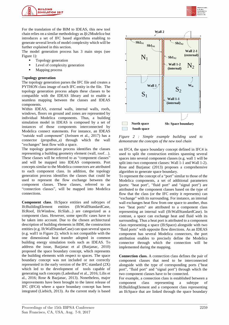
Finally, Figure 7 demonstrates the impact of the different

levels of complexity on the obtained indoor temperature

profiles. Specifically, the living room, kitchen and

bathroom have been chosen as they respectively represent

the dominant space of the South zone, a space of the North

zone with windows oriented West and a space of the

South zone with windows oriented east.

On the one hand, Figure 7 (kitchen) shows that the

increase of the energy use found for LOC4 can be

explained by the higher indoor temperatures that are

obtained in the North zone. Since in the aggregation

process it is assumed that the Northern zone inherit the

heating control of the South zone, the average temperature

in the entire building increases. On the other hand, Figure

7 also demonstrates that aggregation of zones has a

significant impact in analysing thermal comfort. Since for

LOC3 and LOC4, solar gains and the heating power is

allocated to respectively the whole zone or the complete

building, the temperature profile shows smaller

fluctuations. Moreover, problems that may occur in

specific spaces can no longer be evaluated. For example,

in the bathroom, the temperature increase in the morning

of 29-04-2014 is less strong for LOC3 compared to LOC1

and LOC2. Moreover, the peak occurs at a different time,

Figure 5 Comparison of the total energy use for heating

obtained for the different levels of complexity

Figure 6 Load duration curve as function of LOC


2264

since the bathroom is oriented east while most windows

of the South zone are oriented south. Hence for the south

zone the peak temperature occurs in the afternoon. A

similar effect is observed for the kitchen. Nevertheless,

for the kitchen the peak occurs in the evening as it is

oriented west. After aggregation of the spaces in the North

zone, the temperature remains below 23.8°C and doesn’t

reflect the clear peaks (up to 27°C) due to solar gains in

the kitchen. Hence, a correct assessment of overheating

would require a model with individual spaces.

Conclusion

This paper presents a novel tool chain for the direct

coupling between building information models (BIM) and

building energy simulation models (BES) implemented in

Modelica. The new tool chain brings several

improvements over existing methodologies. It alleviates

the limitations of the original Ifc2Modelica tool chain on

which it is based. The major innovation is the introduction

of user controlled flexibility by facilitating the generation

of BES models with different levels of complexity. Where

existing BIM to BES tools offer a one-on-one mapping of

building components to BES models, this work includes

rules for aggregating spaces and building components,

which can be of high importance as the complexity and

size of building increases. The later may drastically

reduce the modelling work needed during different stages

of the design process.

In the second part of the paper, the tool chain was

demonstrated and the implementation of the level of

Figure 7 Indoor temperature profiles for the living room, bathroom and kitchen obtained for the different levels of

complexity (LOC1- LOC4)


2265

complexity was verified against a well-documented full-

scale experiment. Results show significant savings in

computation time with limited impact on accuracy when

zones are grouped according to control strategy.

Nevertheless, further research is needed on a wider range

of buildings before generalisation is possible. Moreover,

based on the findings of this case study, some interesting

points for future research were identified. For instance, in

line with the aggregation of the physical components,

aggregation rules for ‘boundary conditions’ such as

control and occupant behaviour could reduce the gap

between LOC3 and LOC4.

Acknowledgement

This project receives the support of the European Union,

the European Regional Development Fund ERDF,

Flanders Innovation & Entrepreneurship and the Province

of Limburg.

References

Andriamamonjy, A., Klein, R. & Saelens, D. (2016).

IFC-assisted building energy performance

simulation implementation. Development of a

python package. In: Proceedings of the 3rd

IBPSA-England Conference, Newcastle, 12th-14th

September 2016, 1094. 2016.

Baetens, R., De Coninck, R., Jorissen, F., Picard, D.,

Helsen, L. & Saelens, D. (2015). OpenIDEAS - An

Open Framework for Integrated District Energy

Assessment. Proceedings of the 14th IBPSA

Conference - Building Simulation 2015.

(November).

Bazjanac, V. (2010). Space boundary requirements for

modeling of building geometry for energy and

other performance simulation. In: Proceedings of

the CIB W78 2010: 27th International Conference

–Cairo, Egypt, 16-18 November. 2010.

CEN (2016) EN ISO 16739:2016: Industry Foundation

Classes (IFC) for data sharing in the construction

and facility management industries

Crawley, D.B., Lawrie, L.K., Winkelmann, F.C., Buhl,

W.F., Huang, Y.J., Pedersen, C.O., Strand, R.K.,

Liesen, R.J., Fisher, D.E., Witte, M.J. & Glazer, J.

(2001). EnergyPlus : creating a new-generation

building energy simulation program. Energy &

Buildings. 33. p.pp. 319–331.

Dimitriou, V., Firth, S., Hassan, T. & Fouchal, F. (2016).

BIM enabled building energy modelling :

development and veri cation of a GBXML to IDF

conversion method. In: Proceedings of the 3rd

IBPSA-England Conference, Newcastle, 12th-14th

September 2016, 1126. 2016.

Hafele, K.-H., Geiger, A. & Liebich, T. (2013).

Coordination View Version 2 . 0 for IFC 2x3.

[Online]. Available from:

http://www.buildingsmart-

tech.org/downloads/view-definitions/coordination-

view/sub-

schema/CoordinationView_V20_EntityList_IFC2x

3_Version16_Final.pdf.

Hietanen, J. (2008). IFC Model View Definition Format.

[Online]. 2008. Available from:


tech.org/downloads/accompanying-

documents/formats/mvdxml-

documentation/MVD_Format_V2_Proposal_0801

28.pdf

Jeong, W., Kim, J.B., Clayton, M.J., Haberl, J.S. & Yan,

W. (2014). Translating Building Information

Modeling to Building Energy Modeling Using

Model View Definition. Hindawi Publishing

Corporation, The Scientific World Journal. 2014

(1).

Jeong, W., Kim, J.B., Clayton, M.J., Haberl, J.S., Yan,

W. (2016). A framework to integrate object-

oriented physical modelling with building

information modelling for building thermal

simulation. Journal of Building Performance

Simulation. 9 (January). p.pp. 50–69.

Jorissen, F., Baetens, R. & Picard, D. (2017). IDEAS

v1.0.0. [Online]. 2017. Available from:

https://github.com/open-ideas/IDEAS.

Kim, H., Shen, Z., Kim, I., Kim, K., Stumpf, A. & Yu, J.

(2016). BIM IFC information mapping to building

energy analysis ( BEA ) model with manually

extended material information. Automation in

Construction. 68. p.pp. 183–193.

Krijnen, T., Kämäräinen, A. (2015). IfcOpenShell.

[Online]. 2015. Available from:

https://github.com/IfcOpenShell/IfcOpenShell.

Ladenhauf, D., Battisti, K., Berndt, R., Eggeling, E.,

Fellner, D.W., Gratzl-michlmair, M. & Ullrich, T.

(2016). Computational geometry in the context of

building information modeling. Energy &

Buildings. [Online]. 115. p.pp. 78–84. Available

from:

http://dx.doi.org/10.1016/j.enbuild.2015.02.056.

Liebich, T. (2013). IFC4 – the new buildingSMART

Standard. [Online]. Available from:


tech.org/specifications/ifc-releases/ifc4-

release/buildingSMART_IFC4_Whatisnew.pdf.

Liebich, T., Adachi, Y., Forester, J., Hyvarinen, J.,

Richter, S., Chipman, T., Weise, M. & Wix, J.

(2017). ifcDoc Tool Summary. [Online]. 2017.

Available from: http://www.buildingsmart-

tech.org/specifications/specification-tools/ifcdoc-

tool.

Liebich, T. & Chipman, T. (2015). Industry Foundation

Classes, Version 4 - Addendum 1. [Online]. 2015.

Available from: http://www.buildingsmart-

tech.org/ifc/IFC4/Add1/html/. [Accessed: 3 March

2017].

Lilis, G.N., Giannakis, G.I. & Rovas, D. V (2016).

Automatic generation of second-level space

boundary topology from IFC geometry inputs.

Automation in Construction. [Online]. Available

from:

http://dx.doi.org/10.1016/j.autcon.2016.08.044.


2266

Pinheiro, S., O’Donnell, J., Wimmer, R., Bazjanac, V.,

Muhic, S., Maile, T., Frisch, J. & Van Treeck, C.

(2016). Model View Definition for Advanced

Building Energy Performance Simulation. In:

Proceedings of the CESBP Central European

Symposium on Building Physics / BauSIM 2016.

2016.

Remmen, P., Cao, J., Ebertshäuser, S., Frisch, J.,

Lauster, M., Maile, T., Müller, D. & Treeck, C.

Van (2015). An open framework for integrated

BIM-based building performance simulation using

Modelica. Proceedings of the 14th IBPSA

Conference - Building Simulation 2015.

Reynders, G. (2015) Quantifying the impact of building

design on the potential of structural storage for

active demand response in residential buildings.

PhD thesis, KU Leuven, Building Physics Section.

Rose, C.M. & Bazjanac, V. (2013). An algorithm to

generate space boundaries for building energy

simulation. Engineering with Computers. 31. p.pp.

271–280.

Strachan, P., Monari, F., Kersken, M. & Heusler, I.

(2015). IEA Annex 58 : Full-scale Empirical

Validation of Detailed Thermal Simulation

Programs. Energy Procedia. [Online]. 78. p.pp.

3288–3293. Available from:

http://dx.doi.org/10.1016/j.egypro.2015.11.729.

Strachan, P., Svehla, K., Kersken, M. & Heusler, I.

(2016). IEA EBC Annex 58 - Report of Subtask 4a:

Emperical validation of common building energy

simulation models based on in situ dynamic data.

[Online]. Available from:

https://www.kuleuven.be/bwf/projects/annex58/dat

a/A58_Final_Report_ST4a.pdf.

Thorade, M., Rädler, J., Remmen, P., Maile, T.,

Wimmer, R., Cao, J., Lauster, M., Dirk, C.N. &

Christoph, M. (2015). An open toolchain for

generating Modelica code from Building

Information Models. In: Proceedings of the 11th

International Modelica Conference September 21-

23, 2015, Versailles, France. 2015.

Wetter, M. (2009). Modelica-based modelling and

simulation to support research and development in

building energy and control systems. Journal of

Building Performance Simulation. 2 (june). p.pp.

143–161.

Documents

(a ) LOC1 LOC2 LOC3 LOC4 Towards an IFC-Modelica … · 1KU Leuven, Department of Civil Engineering, Building Physics Section, ... or level of detail, ... A first part of this paper