A Logical Account of Causal and Topological Maps

by

Emilio Remolina, M.S.

Dissertation

Presented to the Faculty of the Graduate School of

The University of Texas at Austin

in Partial Fulfillment

of the Requirements

for the Degree of

Doctor of Philosophy

The University of Texas at Austin

December 2001

A Logical Account of Causal and Topological Maps

Publication No.

Emilio Remolina, Ph.D.The University of Texas at Austin, 2001

Supervisor: Benjamin Kuipers

The Spatial Semantic Hierarchy (SSH) is a set of distinct representations for large scalespace, each with its own ontology and each abstracted from the levels below it. At thecontrol level, the agent and its environment are modeled as continuous dynamical systemswhose equilibrium points are abstracted to a discrete set of distinctive states. The controllaws whose execution defines trajectories linking these states are abstracted to actions, giv-ing a discrete causal graph representation for the state space. The causal graph of states andactions is in turn abstracted to a topological network of places and paths (i.e. the topologicalmap). Local metrical models of places and paths can be built within the framework of thecontrol, causal and topological levels while avoiding problems of global consistency.

Most of the SSH’s ideas have been traditionally described in procedural terms in-spired by implementations of the SSH. This description has various problems when used toimplement physical agents. First, some assumptions are not explicitly stated or are difficultto meet by current sensory technology (e.g. sensory information is not rich enough to dis-tinguish one place from another). Second, some important SSH concepts (i.e. paths) arenot properly defined or understood. Third, sometimes it is not clear what the representationstates and consequently it is hard to apply it to new domains.

In this dissertation we propose a formal semantics for the SSH causal, topologicaland local metrical theories. Based on this semantics, we extend the SSH in the followingimportant ways: i) we include distinctive states as objects of the theory and handle per-ceptual aliasing, ii) we define the models associated with the SSH causal and topological

ii

levels, iii) we extend the SSH topological theory to handle convergent and self intersectingpaths as well as hierarchical maps , iv) we show how to combine causal, topological andnoisy local metrical information, v) based on the previous enhancements, we define an al-gorithm to keep track of different topological maps consistent with the agent’s experiences.This algorithm supports different exploration strategies and facilitates map disambiguationwhen the case arises.

iii

Contents

Abstract ii

Chapter 1 Dissertation Overview 1

Chapter 2 SSH Overview 62.1 The Spatial Semantic Hierarchy . . . . . . . . . . . . . . . . . . . . . . . 62.2 Creating Schemas . . . . . . . . . . . . . . . . . . . . . . . . . . . . . . . 82.3 The SSH topological level: regions . . .. . . . . . . . . . . . . . . . . . . 92.4 Physical Implementation of the SSH . . . . . . . . . . . . . . . . . . . . . 10

Chapter 3 Control Level 123.1 SSH control assumptions. . .. . . . . . . . . . . . . . . . . . . . . . . . . 13

3.1.1 The SSH control closure property . . . . . . . . . . . . . . . . . . 133.1.2 Well separated dstate . . . . . . . . . . . . . . . . . . . . . . . . . 133.1.3 From control laws to actions . . . . . . . . . . . . . . . . . . . . . 14

3.2 Voronoi robots . .. . . . . . . . . . . . . . . . . . . . . . . . . . . . . . 14

Chapter 4 Causal Level 164.1 Causal level Ontology . . . . . . . . . . . . . . . . . . . . . . . . . . . . . 17

4.1.1 Views . . . . . . . . . . . . . . . . . . . . . . . . . . . . . . . . . 174.1.2 Actions . . . . . . . . . . . . . . . . . . . . . . . . . . . . . . . . 174.1.3 Distinctive States . . . . . . . . . . . . . . . . . . . . . . . . . . . 194.1.4 Schemas . . . . . . . . . . . . . . . . . . . . . . . . . . . . . . . 194.1.5 Schema notation . . . . . . . . . . . . . . . . . . . . . . . . . . . 204.1.6 Routines . . . . . . . . . . . . . . . . . . . . . . . . . . . . . . . 20

4.2 SSH Causal theory . . . . . . . . . . . . . . . . . . . . . . . . . . . . . . 214.2.1 The E formulae. . . . . . . . . . . . . . . . . . . . . . . . . . . . 214.2.2 The SSH view graph . . . . . . . . . . . . . . . . . . . . . . . . . 24

iv

4.2.3 CT(E) . . . . . . . . . . . . . . . . . . . . . . . . . . . . . . . . . 264.3 The SSH causal graph . . . . . . . . . . . . . . . . . . . . . . . . . . . . . 314.4 Calculating the models of CT(E) . . . . . . . . . . . . . . . . . . . . . . . 324.5 Summary . . . . . . . . . . . . . . . . . . . . . . . . . . . . . . . . . . . 34

Chapter 5 Topological Level 365.1 The SSH Topological Theory. . . . . . . . . . . . . . . . . . . . . . . . . 375.2 teq versusceq . . . . . . . . . . . . . . . . . . . . . . . . . . . . . . . . . 585.3 The SSH topological map . .. . . . . . . . . . . . . . . . . . . . . . . . . 595.4 What if Views uniquely identify distinctive states. . . . . . . . . . . . . . 605.5 Coping with self intersecting paths . . . . . . . . . . . . . . . . . . . . . . 63

5.5.1 Converging paths . . . . . . . . . . . . . . . . . . . . . . . . . . . 645.5.2 Self-intersecting paths. . . . . . . . . . . . . . . . . . . . . . . . 645.5.3 New circumscription policy . . . . . . . . . . . . . . . . . . . . . 655.5.4 Explicit definitions . . . . . . . . . . . . . . . . . . . . . . . . . . 685.5.5 General SSH topological theory. . . . . . . . . . . . . . . . . . . 69

5.6 Calculating the models of TT(E) . . . . . . . . . . . . . . . . . . . . . . . 715.7 Summary . . . . . . . . . . . . . . . . . . . . . . . . . . . . . . . . . . . 75

Chapter 6 Boundary Regions 776.1 Qualitative orientation of paths at a place. . . . . . . . . . . . . . . . . . 796.2 Left and Right of a path . . . . . . . . . . . . . . . . . . . . . . . . . . . . 79

6.2.1 Adding boundary relations to the topological map . .. . . . . . . . 826.3 Summary . . . . . . . . . . . . . . . . . . . . . . . . . . . . . . . . . . . 88

Chapter 7 Using Metrical Information 907.1 Schemas, representing uncertainty . . .. . . . . . . . . . . . . . . . . . . 917.2 Frames of reference . . . . . . . . . . . . . . . . . . . . . . . . . . . . . . 92

7.2.1 One dimensional frames of reference . . . . . . . . . . . . . . . . 927.2.2 Radial frames of reference . . . . . . . . . . . . . . . . . . . . . . 947.2.3 Two dimensional frames of reference . . . . . . . . . . . . . . . . 96

7.3 Combining topological and metrical information .. . . . . . . . . . . . . . 977.4 Creating two dimensional frames of reference . . . . . . . . . . . . . . . . 102

7.4.1 When to create two dimensional frames of reference . . . . . . . . 1027.4.2 How to create two dimensional frames of reference . . . . . . . . . 1037.4.3 “Mental” route rehearsal . . . . . . . . . . . . . . . . . . . . . . . 1047.4.4 Combining information from multiple routes. . . . . . . . . . . . 106

7.5 Summary . . . . . . . . . . . . . . . . . . . . . . . . . . . . . . . . . . . 111

v

Chapter 8 Regions 1138.1 Including regions in the SSH topological level . .. . . . . . . . . . . . . . 113

8.1.1 Defining paths among regions . . . . . . . . . . . . . . . . . . . . 1148.1.2 One dimensional frames of reference associated with routes . . . . 1208.1.3 Radial frames of reference associated with regions .. . . . . . . . 121

8.2 Creating Regions . . . . . . . . . . . . . . . . . . . . . . . . . . . . . . . 1228.3 Using regions to solve spatial problems . . . . . . . . . . . . . . . . . . . 1248.4 Summary . . . . . . . . . . . . . . . . . . . . . . . . . . . . . . . . . . . 126

Chapter 9 Implementation 1289.1 Vulcan . . . . . . . . . . . . . . . . . . . . . . . . . . . . . . . . . . . . . 1299.2 Control laws . . . . . . . . . . . . . . . . . . . . . . . . . . . . . . . . . . 130

9.2.1 Following a wall/corridor. . . . . . . . . . . . . . . . . . . . . . . 1319.2.2 Going through doorways. . . . . . . . . . . . . . . . . . . . . . . 1339.2.3 Hill Climbing . . . . . . . . . . . . . . . . . . . . . . . . . . . . . 134

9.3 Views . . . . . . . . . . . . . . . . . . . . . . . . . . . . . . . . . . . . . 1389.3.1 Line segment extraction . . . . . . . . . . . . . . . . . . . . . . . 142

9.4 Causal/Topological/Metrical levels . . .. . . . . . . . . . . . . . . . . . . 1479.4.1 Using Logic Programming to implement the SSH causal level . . . 1479.4.2 Calculating the models of TT(E) . . . . . . . . . . . . . . . . . . . 1529.4.3 Trace example . . . . . . . . . . . . . . . . . . . . . . . . . . . . 161

9.5 Map building examples . . . . . . . . . . . . . . . . . . . . . . . . . . . . 1699.5.1 Rectangular environment. . . . . . . . . . . . . . . . . . . . . . . 1699.5.2 Taylor’s Second floor . . . . . . . . . . . . . . . . . . . . . . . . . 176

9.6 Summary . . . . . . . . . . . . . . . . . . . . . . . . . . . . . . . . . . . 181

Chapter 10 Related Work 18310.1 Cognitive theories of space representation. . . . . . . . . . . . . . . . . . 183

10.1.1 PLAN . . . . . . . . . . . . . . . . . . . . . . . . . . . . . . . . . 18310.1.2 McDermott and Davis . . . . . . . . . . . . . . . . . . . . . . . . 184

10.2 Cognitive Robotics . . . . . . . . . . . . . . . . . . . . . . . . . . . . . . 18510.2.1 GOLOG . . . . . . . . . . . . . . . . . . . . . . . . . . . . . . . . 18510.2.2 Shanahan’s Work . . . . . . . . . . . . . . . . . . . . . . . . . . . 186

10.3 Qualitative Representation of Space . .. . . . . . . . . . . . . . . . . . . 18710.4 Robotics . . . . . . . . . . . . . . . . . . . . . . . . . . . . . . . . . . . . 189

10.4.1 Metrical maps . . . . . . . . . . . . . . . . . . . . . . . . . . . . . 18910.4.2 Fuzzy control . . . . . . . . . . . . . . . . . . . . . . . . . . . . . 18910.4.3 Probabilistic navigation. . . . . . . . . . . . . . . . . . . . . . . 190

vi

Chapter 11 Conclusions and Future Work 19111.1 Future work . . . . . . . . . . . . . . . . . . . . . . . . . . . . . . . . . . 193

11.1.1 Extension for the current theory . . . . . . . . . . . . . . . . . . . 19311.1.2 Learning the control level . . . . . . . . . . . . . . . . . . . . . . 19411.1.3 Open environments . . . . . . . . . . . . . . . . . . . . . . . . . . 19411.1.4 Reasoning with multiple spatial representations . . .. . . . . . . . 195

Appendix A Using the SSH 196A.1 Location . . . . . . . . . . . . . . . . . . . . . . . . . . . . . . . . . . . . 196

A.1.1 Representing location knowledge. . . . . . . . . . . . . . . . . . 197A.1.2 Probabilistic representations of location .. . . . . . . . . . . . . . 203

A.2 Planning . . . . . . . . . . . . . . . . . . . . . . . . . . . . . . . . . . . . 206A.2.1 Using topological paths for planning . . .. . . . . . . . . . . . . . 206A.2.2 Using regions for planning . . . . . . . . . . . . . . . . . . . . . . 207A.2.3 Conventional planners . . . . . . . . . . . . . . . . . . . . . . . . 208

A.3 Navigation . . . . . . . . . . . . . . . . . . . . . . . . . . . . . . . . . . . 208A.4 Summary . . . . . . . . . . . . . . . . . . . . . . . . . . . . . . . . . . . 212

Appendix B Topological Level Properties 214

Appendix C Nested Abnormality theories 219C.1 Nested Abnormality theories (NAT’s) .. . . . . . . . . . . . . . . . . . . 222

Appendix D Answer Sets 226

Appendix E Ceq Properties 229

Appendix F Logic Program Correctness 236

Appendix G MERCATOR’s Ontology and Semantics 243

Bibliography 246

Vita 256

vii

Chapter 1

Dissertation Overview

The Spatial Semantic Hierarchy (SSH)[Kuipers and Byun, 1988, Kuipers and Byun, 1991,Kuipers, 1996, Kuipers, 2000] is a set of distinct representations for large scale space,1 eachwith its own ontology, each with its own mathematical foundation, and each abstracted fromthe levels below it. The SSH is a computational theory of the cognitive map (i.e. humanknowledge of large-scale space). The SSH is used in robotics to supportmap buildingandnavigation. Using the SSH representation, navigation among places is not dependent on theaccuracy, or even the existence, of metrical knowledge of the environment.

The SSH describes the different states of knowledge that an agent uses in order toorganize its sensorimotor experiences and create a spatial representation (i.e. a map). TheSSH gives an account of how continuous interaction with the world is abstracted to a dis-crete spatial representation. Next we describe how the different levels of the SSH (control,causal, topological and metrical) accomplish this.

At the SSH control level, the agent and its environment are modeled as continuousdynamical systems whose equilibrium points are abstracted to a discrete set ofdistinctivestates. A distinctive state has an associatedview describing the sensory input obtained atthat distinctive state. The control laws whose execution defines trajectories linking thesedistinctive states can be abstracted toactions, giving a discrete causal graph representationfor the state space. The causal graph of states and actions can in turn be abstracted to atopological network ofplacesandpaths(i.e. the topological map). Local metrical models,such as occupancy grids, of places and paths can then be built on the framework of the

1In large-scale space the structure of the environment is revealed by integrating local observations over time,rather than being perceived from a single vantage point.

1

topological network while avoiding problems of global consistency.2

Our goal is to define the SSH so that it is clear how it can be implemented acrossdifferent robot platforms as well as in other domains. In principle, in order to implementthe SSH on a given robot, it should be enough to define the robot’s trajectory-followingand hill-climbing control laws, to define views, and to show how the local metrical mapis derived from sensory input. A well defined interface between the SSH and the robot’scontrol system allows the SSH control level to identify distinctive states and actions linkingthem. This information is then propagated to the other levels of the SSH. Under this vision,the SSH will be a well-defined module that can be used by any robot. Unfortunately, theexisting formulation of the SSH is not at this point yet.

Part of the difficulty when implementing the SSH is to extract world informa-tion through sensors. Advances in hardware and robotics, as well as experience gainedfrom previous SSH implementations[Lee, 1996], allow us to deal with sensor unrelia-bility and implement robust control laws. As control laws are the ones that ultimatelymake a robot move, it is not surprising that there has been much work on implement-ing the SSH control level. A side effect of this effort has been that sometimes it is notclear what is and what is not part of the SSH. For example, in[Kuipers and Byun, 1988,Lee, 1996] the robot’s exploration strategy is part of the SSH control level, though the orig-inal SSH’s description aims for constructing the SSH opportunistically, independent of howactions are selected and executed by the robot.

Most of the key concepts in the SSH framework have been traditionally describedin procedural terms inspired by implementations of the SSH. This description has variousproblems when used to implement physical agents. First, some assumptions are not explic-itly stated or are difficult to meet by current sensory technology (i.e. sensory informationis not rich enough as to distinguish one place from another). Second, some important SSHconcepts (i.e. paths) are not properly defined or understood. Third, sometimes it is not clearwhat the representation states and consequently it is hard to apply it to new domains.

The goal of this dissertation is to formalize the SSH causal and topological levels inorder to have a clear specification of what the SSH accounts for. We define the SSH causaland topological models (maps) associated with a set of agent’s experiences. These modelsare the spatial representation the agent creates in order to explain such experiences. Howthe agent explores the environment or builds such models are not part of the SSH theory.

2See chapter 2 for a detailed overview of the SSH.

2

Nevertheless, once we present the theory, we illustrate the effect of the exploration strategyas well as present algorithms to build the SSH causal and topological maps.

We start our formalization by includingdistinctive statesas objects of the causaland topological theory. At the SSH control level distinctive states are the fixed points ofhill climbing control laws. At the causal and topological levels distinctive states are objectsrepresenting such fixed points the agent visits at the control level. Part of the purpose of thecausal and topological theories is to determine when two distinctive states refer to the sameenvironment state.

Previous descriptions of the SSH do not include distinctive states as objects of thetheory. This is the case because these descriptions assume that perceptual aliasing (i.e. dif-ferent distinctive states that share the same view) does not occur. Should this hypothesisnot be the case, the agent’s exploration strategy has to handle any environment states disam-biguation. This mix between the SSH description and the robot exploration strategy madeit difficult to state what the SSH itself is about.

In this dissertation we show that by including distinctive states as first order objectsof the theory it is possible to handle perceptual aliasing while formulating the spatial repre-sentation (the SSH) independently of the agent’s exploration strategy. For this purpose weexplicitly define the models of the causal and topological theories associated with a set ofagent’s experiences. Should the experiences not be complete or perceptual aliasing occur,different models of the theory may exist. In such cases, as part of the exploration strategy,the agent could choose to refute some of these models or just keep exploring the environ-ment gathering more experiences.

One interesting aspect of spatial knowledge that becomes clear with the SSH for-malization is thenon-monotoniceffect of gathering more experiences. New informationcould prove environment states to be different although they were previously believed equal,and viceversa. This remark applies not only to environment states but also to other SSH ob-jects like placesand paths. It is not surprising then that we use a non-monotonic logicformalism, namely Nested Abnormalities Theories (NATs)[Lifschitz, 1995], in order tostate the SSH causal and topological theories.

A logical account of the SSH causal, topological and local metrical theories is givenusing NATs. The minimality conditions embedded in the formalization define the preferredmodels associated with the theories. In chapters 4 through 8 we illustrate the main prop-

3

erties of the new theories. In particular we show how the minimal models associated withthese theories are adequate models for the spatial knowledge an agent has about its envi-ronment. We also illustrate how the different levels of the representation assume differentspatial properties about both the environment and the actions performed by the agent. Thesespatial properties play the role of “filters” the agent applies in order to distinguish the dif-ferent environment states it has visited.

As part of our formalization, we have chosen to explicitly represent when two dis-tinctive states denote the same environment state. The predicatesceq andteq (chapters 4and 5) denote when two distinctive states are equal given causal and topological informa-tion, respectively.ceq is the case when it is not possible to distinguish distinctive statesby views (sensory input) and actions.teq is the case when distinctive states have the sameview and are at the same place along the same paths. While the topological ontology (thatof places and paths) is more elaborated than the one for the causal level, it is easier to buildthis representation than it is to distinguish environment states based only on view-action-view sequences.

At the SSH causal level we introduced a new spatial representation, that of thecausal graph. A causal graph is a deterministic finite automaton (DFA) where states areceq

equivalence classes, and transitions correspond to actions. In the presence of perceptualaliasing this representation is different from theview graph, a non-deterministic automatonwhere states are views, and transitions are actions. In chapter 4 we elaborate on the proper-ties of this representation.

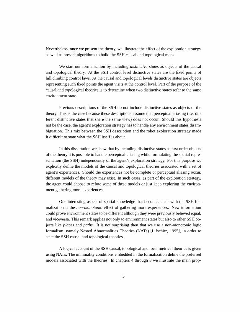
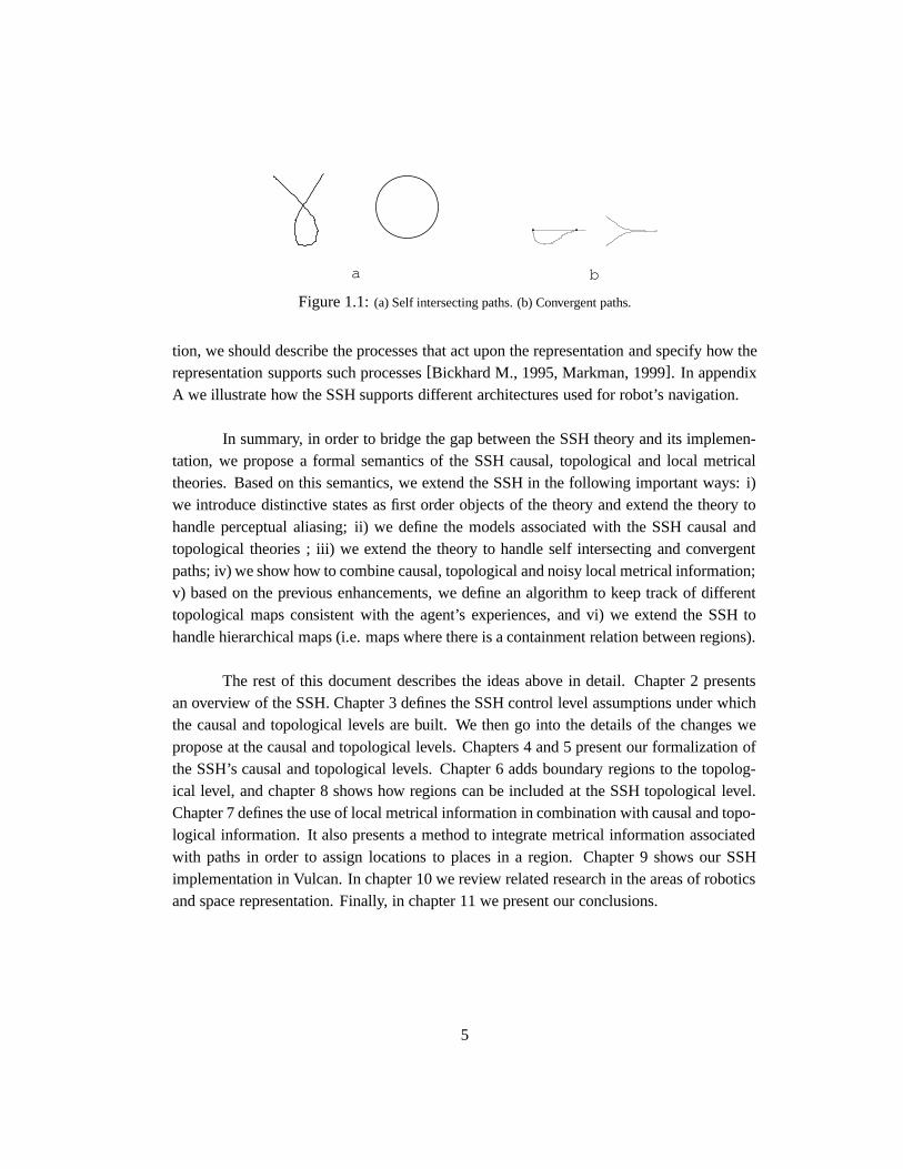
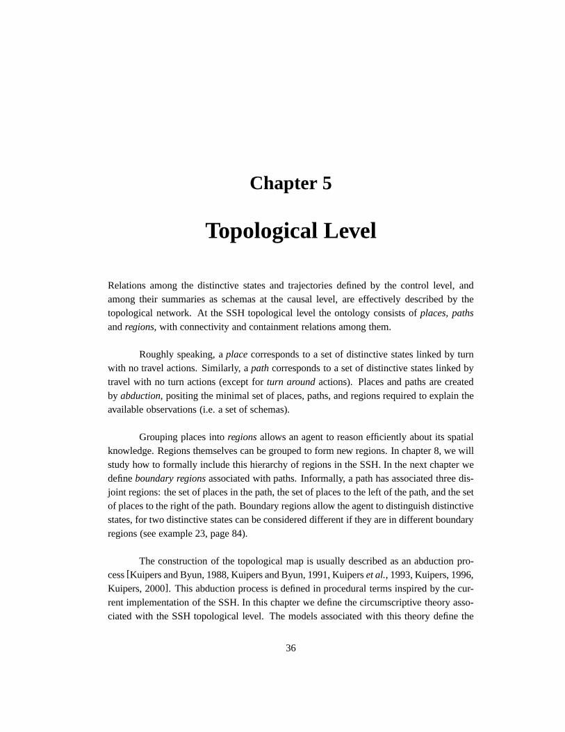
The SSH topological theory is presented in chapters 5 through 8. We start with asimple topological theory that assumes “simple” paths in the environment. We then extendthe theory to handle more complex paths, namely self-intersecting and convergent paths(figure 1.1). We then extend the theory with boundary regions, local metrical informationand finally, abstraction regions. At each step, we illustrate how the new spatial represen-tation allows the agent to distinguish environments not distinguishable with the previousrepresentations. Based on the SSH causal and topological formalizations, we define analgorithm that allows the agent to keep track of different models consistent with a set ofexperiences.

As the ultimate goal of this work is to show that a formal specification of the SSHwill facilitate its implementation on physical robots, we evaluated our methods by imple-menting the SSH in Vulcan, our wheelchair robot (chapter 9). As with any other representa-

4

a b

Figure 1.1:(a) Self intersecting paths. (b) Convergent paths.

tion, we should describe the processes that act upon the representation and specify how therepresentation supports such processes[Bickhard M., 1995, Markman, 1999]. In appendixA we illustrate how the SSH supports different architectures used for robot’s navigation.

In summary, in order to bridge the gap between the SSH theory and its implemen-tation, we propose a formal semantics of the SSH causal, topological and local metricaltheories. Based on this semantics, we extend the SSH in the following important ways: i)we introduce distinctive states as first order objects of the theory and extend the theory tohandle perceptual aliasing; ii) we define the models associated with the SSH causal andtopological theories ; iii) we extend the theory to handle self intersecting and convergentpaths; iv) we show how to combine causal, topological and noisy local metrical information;v) based on the previous enhancements, we define an algorithm to keep track of differenttopological maps consistent with the agent’s experiences, and vi) we extend the SSH tohandle hierarchical maps (i.e. maps where there is a containment relation between regions).

The rest of this document describes the ideas above in detail. Chapter 2 presentsan overview of the SSH. Chapter 3 defines the SSH control level assumptions under whichthe causal and topological levels are built. We then go into the details of the changes wepropose at the causal and topological levels. Chapters 4 and 5 present our formalization ofthe SSH’s causal and topological levels. Chapter 6 adds boundary regions to the topolog-ical level, and chapter 8 shows how regions can be included at the SSH topological level.Chapter 7 defines the use of local metrical information in combination with causal and topo-logical information. It also presents a method to integrate metrical information associatedwith paths in order to assign locations to places in a region. Chapter 9 shows our SSHimplementation in Vulcan. In chapter 10 we review related research in the areas of roboticsand space representation. Finally, in chapter 11 we present our conclusions.

5

Chapter 2

SSH Overview

2.1 The Spatial Semantic Hierarchy

The Spatial Semantic Hierarchy (SSH)[Kuipers and Byun, 1988, Kuipers and Byun, 1991,Kuiperset al., 1993, Kuipers, 1996, Kuipers, 2000]1 is anontological hierarchyof represen-tations for knowledge of large-scale space. An ontological hierarchy shows how multiplerepresentations for the same kind of knowledge can coexists. Each level of the hierarchyhas its ownontology(the set of objects and relations it uses for describing the world) and itsown set of inference and problem-solving methods. The objects, relations, and assumptionsrequired by each level are provided by those below it.

The SSH abstracts the structure of an agent’s spatial knowledge in a way that isrelatively independent of its sensorimotor apparatus and the environment within which itmoves. Next we describe the different SSH levels.

� The sensorimotor levelof the agent provides continuous sensors and effectors, butnot direct access to the global structure of the environment, or the robot’s position ororientation within it.

� At the control levelof the hierarchy, the ontology is an egocentric sensorimotor one,without knowledge of fixed objects or places in an external environment. Adistinc-tive stateis defined as the local maximum found by a hill-climbing control strategy,climbing the gradient of a selected feature, ordistinctiveness measure. Trajectory-following control laws take the robot from one distinctive state to the neighborhoodof the next, where hill-climbing can find a local maximum, reducing position errorand preventing its accumulation.

1This presentation follows[Kuipers, 1996].

6

� The ontology at the SSHcausal levelconsists of views, distinctive states, actions andschemas. Aview is a description of the sensory input obtained at a locally distinc-tive state. Anaction denotes a sequence of one or more control laws which can beinitiated at a locally distinctive state, and terminates after a hill climbing control lawwith the robot at another distinctive state. Aschemais a tupleh (V; dp); A; (V 0; dq) irepresenting the (temporally extended) event in which the robot takes a particular ac-tionA, starting with viewV at the distinctive statedp, and terminating with viewV 0

at distinctive statedq. The spatial representation posits the minimal set of distinctivestates consistent with the set of schemas.

� At the topological levelof the hierarchy, the ontology consists ofplaces, pathsandre-gions, with connectivity and containment relations. The spatial representation positsthe minimum set of paths and places consistent with the set of causal schemas.2 Atthe SSH topological level, action symbols are categorized in two classes:Turn andTravel. A place corresponds to a set of distinctive states linked by turn actions. A pathis a structure that includes an ordered sequence of places connected by travel actionswithout turns. Paths are used in the cognitive map to describe linear geographicalstructures such as streets. Places and paths define a topological network which canbe used to guide exploration of new environments and to solve new route-findingproblems.3 Using the network representation, navigation among distinctive states isnot dependent on the accuracy, or even the existence, of metrical knowledge of theenvironment.

� At themetrical levelof the hierarchy, the ontology for places, paths, and sensory fea-tures is extended to include metrical properties such as distance, direction, shape, etc.Geometrical features are extracted from sensory input, and represented as annotationson the places and paths of the topological network.

Two fundamental ontological distinctions are embedded in the SSH. First, the con-tinuous world of the sensorimotor and control levels is abstracted to the discrete symbolicrepresentation at the causal and topological levels, to which the metrical level adds contin-uous properties. Second, the egocentric world of the sensorimotor, control, and causal levelis abstracted to the world-centered ontologies of the topological and metrical levels.

2In order to state these minimality conditions, the causal and topological levels are formalized as circum-scriptive theories (see chapter 5).

3Notice that although the topological map has a graph like structure, a path in the graph theory sense is notnecessarily a SSH topological path.

7

2.2 Creating Schemas

As the agent navigates its environment, a set of schemas summarizing its experiences iscreated. This set of schemas is the only source of information the agent has to create aspatial representation of its environment. Next we describe how a set of schemas is createdas the agent navigates through its environment.

At the SSH control level, exploration is performed by alternating execution be-tween two types of continuous control strategies,4trajectory-followingandhill-climbing .These two types of control strategy differ in their roles: ahill-climbing control strategy isfor climbing towards a local maximum of a distinctiveness measure and thus a position ofsome distinctive state; atrajectory-followingcontrol strategy is for moving from the neigh-borhood of one distinctive state to the neighborhood of another. The actual motion fromone distinctive state to the neighborhood of another may be the result of the execution ofa sequence of more than one control strategy (see example below). Letcl = cl1; : : : ; clmbe the sequence of control strategies executed at the control level to take the agent fromdistinctive stateds with view V to distinctive stateds0 with view V 0. Then, the schemah(V; ds); A; (V 0; ds0)i is created at the SSH causal level, whereA is anactionsymbol usedwhenever the sequencecl is executed.5 This way, the experiences of the robot within itsenvironment can be described by an alternating sequence of views and actions

(V1; ds1)A1 (V2; ds2) : : : An�1 (Vn; dsn)

which is summarized at the causal level by the set of schemas S,

S = fh (Vi; dsi); Ai; (Vi+1; dsi+1) i : i = 1; : : : ; n� 1g

Example 1

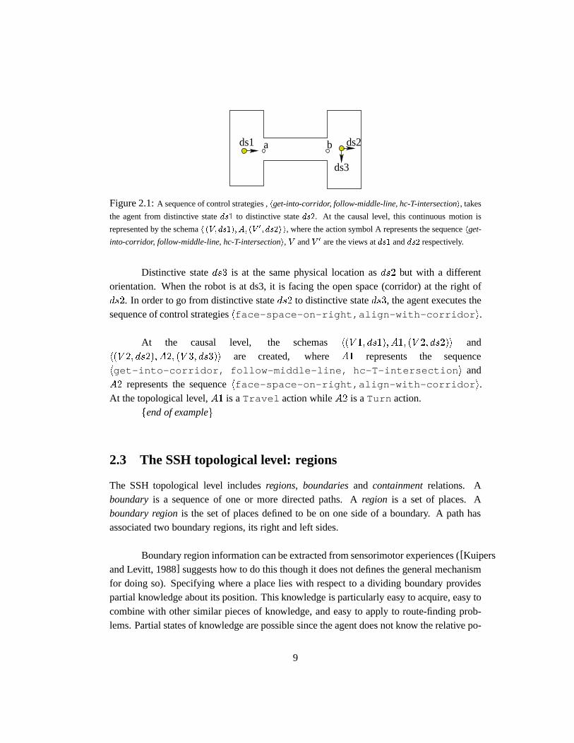
Consider the environment in figure 2.1. In order to go from distinctive stateds1 to distinc-tive stateds2, the agent executes the sequence of control strategieshget-into-corridor,

follow-middle-line, hc-T-intersection iwhereget-into-corridoris a trajectory-following control strategy that moves the agent fromds1 to a, follow-middle-line isa trajectory-following strategy that takes the agent froma tob, andhc-T-intersection

is a hill-climbing control strategy that takes the agent fromb to the distinctive stateds2.Environment statesa andb are not distinctive states. At the distinctive stateds2 the agentis facing the wall ahead and it is equidistant from this wall and the intersection corners.

4These strategies correspond to continuous control laws[Kuo, 1987].5See section 3.1.3, page 14.

8

ds3

ds2bads1

Figure 2.1:A sequence of control strategies ,hget-into-corridor, follow-middle-line, hc-T-intersectioni, takes

the agent from distinctive stateds1 to distinctive stateds2. At the causal level, this continuous motion is

represented by the schemah (V; ds1); A; (V 0; ds2) i, where the action symbol A represents the sequencehget-

into-corridor, follow-middle-line, hc-T-intersectioni, V andV 0 are the views atds1 andds2 respectively.

Distinctive stateds3 is at the same physical location asds2 but with a differentorientation. When the robot is at ds3, it is facing the open space (corridor) at the right ofds2. In order to go from distinctive stateds2 to distinctive stateds3, the agent executes thesequence of control strategieshface-space-on-right,align-with-corridor i.

At the causal level, the schemash(V 1; ds1); A1; (V 2; ds2)i andh(V 2; ds2); A2; (V 3; ds3)i are created, whereA1 represents the sequencehget-into-corridor, follow-middle-line, hc-T-intersection i andA2 represents the sequencehface-space-on-right,align-with-corridor i.At the topological level,A1 is aTravel action whileA2 is aTurn action.

fend of exampleg

2.3 The SSH topological level: regions

The SSH topological level includesregions, boundariesand containmentrelations. Aboundary is a sequence of one or more directed paths. Aregion is a set of places. Aboundary regionis the set of places defined to be on one side of a boundary. A path hasassociated two boundary regions, its right and left sides.

Boundary region information can be extracted from sensorimotor experiences ([Kuipersand Levitt, 1988] suggests how to do this though it does not defines the general mechanismfor doing so). Specifying where a place lies with respect to a dividing boundary providespartial knowledge about its position. This knowledge is particularly easy to acquire, easy tocombine with other similar pieces of knowledge, and easy to apply to route-finding prob-lems. Partial states of knowledge are possible since the agent does not know the relative po-

9

sition of every place with respect to every boundary. Once a sufficient number of boundaryrelations have been accumulated, they provide a useful topological route-finding heuristic.For example, to find a route from A to B, if there is a path such that A is on its right and Bis on its left, look for routes from A to that path and from the path to B. In[Remolina andKuipers, 1998b] we have given a formal account of how boundary relations are establishedas the agent navigates a known environment. In chapter 6 we show how boundary regionsare used while exploring an unknown environment.

2.4 Physical Implementation of the SSH

An implementation of the SSH in a physical robot (Spot) was carried out by W.Y. Lee[Lee,1996]. Most of this work focused on the SSH control level since the other levels can beconstructed as in the TOUR model[Kuipers, 1978].6 Next we review the key ideas in theimplementation.

At the SSH control level, the robot has only an egocentric view of its surroundingswith no concept of external objects. Sensory regularities are the way to identify external ob-jects. Discontinuities in sensory readings mark the presence of distinctive neighborhoods.A SSH robot identify and responds only to sensorimotor regularities at the control level.7

The type of possible distinctive neighborhoods the robot can be at is given a priory.Each of these neighborhoods types has associated a hill climbing strategy as well as a pres-elected order in which distinctive states are visited. Local frames of reference (LFOR) arecreated when visiting a neighborhood. This coordinate system allows the creation of viewsas well as the tracking of corners otherwise not possible from sonar readings. Since thesensory information associated with a neighborhood is not at once available to the robot,the robot has to explore the neighborhood in order to identify the neighborhood’s type. Thisexploration procedure is described by a finite state automaton. Final states in this automatonidentify the type of neighborhood. Transitions in the automaton describe how informationof the neighborhood should be collected and used to discriminate the neighborhood.

In order to choose a hill climbing strategy, the following elements are considered:6Notice that the TOUR model does not account for perceptual aliasing, and it assumes that a unique topo-

logical map is consistent with the agent’s experiences. Any possible ambiguity has to be solved before givingthe schemas to the TOUR algorithm.

7For example, a frontal object is represented internally as a regularity of the changes in frontal sonar mea-surement over time[Lee, 1996].

10

the trajectory-following control strategy that brought Spot into the neighborhood, the eventthat signal the neighborhood (corner or front-blocked), and an analysis of the immediatesurroundings in terms of qualitative positions of frontal objects, if any. The hill climbingstrategies work by applying a trajectory-following control strategy that constrains two de-grees of freedom, and then climbing a distinctive measure in the remaining one degree offreedom until its local maximum is reached. In general the hill climbing strategy is a twostep procedure: first, a distinctive location must be found, and then distinctive orientationsat that location are determined. A distinctive state is a pair(location, orientation). Specialalgorithms to find distinctive orientations were developed. These algorithms deal with errorin sonar readings produced by specularity.

11

Chapter 3

Control Level

At the SSH control level, the agent and its environment are modeled as continuous dynam-ical systems whose equilibrium points are abstracted to a discrete set ofdistinctive states.The agent “moves” from one distinctive state to another, by using a combination oftra-jectory followingand hill climbing control laws. The execution of these control laws isabstracted at the SSH causal level as a set of causal schemas (section 2.2, page 8) fromwhich causal, topological and metrical representations of space are created (chapters 4 to8). Our main hypothesis to build these spatial representations is that the execution of con-trol laws isdeterministicin the following sense: executing a sequence of control laws ata particular environment state leaves the agent “at the same” resulting distinctive state. Inthis chapter we state this property of the SSH control level (the SSHclosure property).

In general it is difficult to prove that a given set of control laws and a particularenvironment satisfy the SSH closure property. A particular case where the closure prop-erty can be proved is for a “Voronoi robot”, a robot that moves along the Voronoi diagramassociated with the environment: the set of points that are equidistant from two nearby ob-jects[Aurenhammer, 1991, Choset and Nagatani, 2001] . In section 3.2 we elaborate in theproperties and limitations of Voronoi robots.

Hill climbing control laws are chosen based on sensory input and (maybe) the tra-jectory following that brought the robot to the current environment state. It may be the casethat different hill climbing control laws bringing the robot to different distinctive statescould be chosen for execution. We would rule out this possibility by requiring distinctivestates to bewell separated(section 3.1.2).

The closure property on the set of control laws and the well separation among dis-

12

tinctive states guarantee that actions at the causal level are deterministic.For the purposeof this dissertation, this is all we need to know about the control level. Next we brieflyelaborate on these SSH control level properties. The reader is referred to[Lee, 1996,Kuipers, 2000] for more detailed information.

3.1 SSH control assumptions.

1Exploration of an unknown environment takes place by selecting a control law based onsensory information available about the local neighborhood. Typically, we expect behaviorto be an alternation betweenhill-climbing control laws, which bring the agent to a locally-distinctive state from any state within the local neighborhood, andtrajectory-followingcon-trol laws, which bring the agent from one distinctive state to the neighborhood of the next.

3.1.1 The SSH control closure property

The navigation strategy of alternating trajectory-following and hill-climbing control lawspresumes that the following criteria are satisfied. We call these theclosure criteriaon theset of control laws.

1. After a hill-climbing control law is executed and terminates at a distinctive state, atleast one trajectory-following control law is available for selection. This ensures thatthere is a choice of action from the current distinctive state: there are no dead end.

2. After a trajectory-following control law is executed and reaches its termination state,at least one hill-climbing control law is available for selection. This ensures that eachtrajectory terminates at a distinctive state.

3.1.2 Well separated dstate

The closure property does not rule out the possibility that more than one hill-climbing maybe available for selection. For the purpose of having deterministic actions at the causallevel, we require that

the basins of attraction of distinctive states are well separated.

This separation property ensure that at most one hill-climbing is available for selectionafter a trajectory following control law is performed. Notice that the basins of attraction of

1In this section we follow[Kuipers, 2000].

13

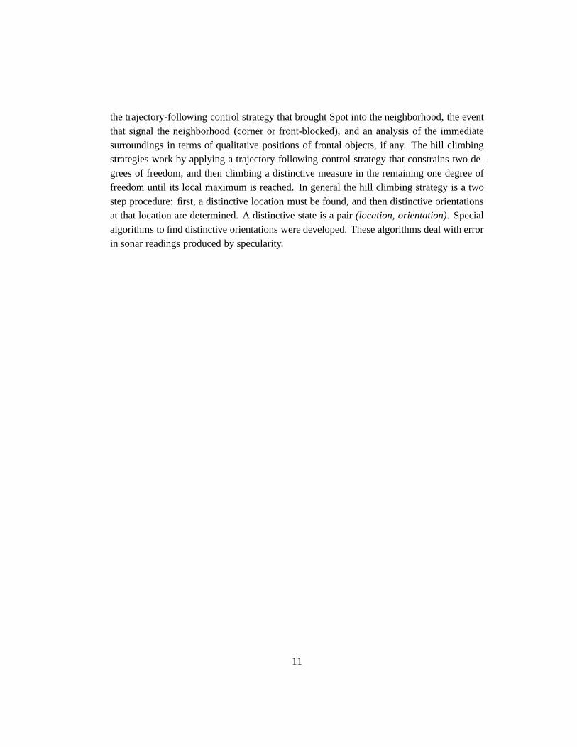
distinctive states could intersect, but in those common environment states the robot has aconsistent “clear choice” of which hill climbing control law to perform (see figure 3.1).

a b

Figure 3.1:Consider a robot coming into an intersection as indicated by the arrow in the figure. Suppose arobot hill climbs to localize itself equidistant from at least three nearby objects. (a) In a “perfect” intersection,the agent will hill climb to the center of the intersection. (b) A small perturbation on the intersection ofa, willcause the robot to have at least two different distinctive states it could reach (indicated by dots in the figure).The SSH well-separated distinctive states property requires the agent to have a clear selection criteria so thatwhen entering the intersection the agent always hill climbs to the same distinctive state.

3.1.3 From control laws to actions

Sequences of control laws are given anaction name at the SSH causal level. In order todecide whether two of such sequences have the same name, we do not consider the lastcontrol law of the sequence (which is required to be a hill climbing control law). Formally,

action(cl1; : : : ; cln) = action(cl01; : : : ; cl0m) iff n = m ^ 8i < n cli = cl0i

whereaction(cl) denotes the action name associated with the sequence of control lawscl.

3.2 Voronoi robots

A Voronoi robot moves along the Voronoi diagram associated with the environment: the setof points that are equidistant from two nearby objects[Choset and Nagatani, 2001]. Voronoirobots are relevant to the SSH control level because they have a well developed mathematicsthat allows one to characterize and prove properties about the control level. Moreover, theyare well understood and different algorithms exist to implement them[Chosetet al., 1997,Choset and Nagatani, 2001]. However, they have two well known limitations. First, smallperturbations in the environment can greatly change the Voronoi diagram (for instance, con-sider the example in figure 3.1). Second, they assume that the robot can perceive at least

14

two nearby objects. This is not the case if the agent only has weak sensors or if objects areoutside the range of the sensors. In this case, control laws that keep the robot equidistantfrom a reference wall are used[Kuipers and Byun, 1988, Lee, 1996].

For the purpose of this dissertation all we need to assume about the SSH controllevel is that its behaviors can be abstracted to deterministic actions at the causal level. Thisis guarantee by satisfying the closure and well-separation properties. Certainly, actionscould fail and so the agent could get lost. We handle these failures during navigation (whenusing an already built map) and assume they do not occur during map building.

15

Chapter 4

Causal Level

The agent’s experiences in the environment are summarized at the SSH causal level byschemas. A schemarepresents an agent’s particular action execution in the environment.An action execution takes the agent from onedistinctive stateto another. Sensory informa-tion at distinctive states is represented byviews.

We can think of a schema as a tuple

h(v; ds); a; (v0; ds0)i

representing the event in which the agent starting at distinctive stateds (whose view isv),executed actiona, terminating at distinctive stateds0 (whose view isv0). It is also possibleto have an incomplete schema where the resulting distinctive state,ds0, is “missing”. Theseincomplete schemas allow the SSH causal level to account for common states of incompleteknowledge like “I could take you there, but I can’t tell you how”[Kuipers, 2000]. In sec-tion 4.1.4 we define how to represent schemas and the information associated with them.We also formally define (see section 4.1.5) a variety of useful “tuple notations”, includingh(v; ds); a; (v0 ; ds0)i, which we will use hereafter.

Schemas can be used to direct the agent behavior in the environment, to distin-guish distinctive states, or as a basis for more elaborated spatial representations. In thefirst case, for example, if the agent’s current view isv and it has experienced a schemah(v; ds); a; (v0 ; ds0)i, it could executea and expect to observev0 [Kuipers, 2000]. In thesecond case, by considering view-action-view sequences, the agent can distinguish distinc-tive states that share the same view (see section 4.2.3). Finally, in chapter 5 we show howby adding some spatial interpretation to the actions executed by the agent, we can build a

16

spatial representation from a set of schemas (the SSH topological map).

This chapter is organized as follows: section 4.1 presents the causal level ontology.We then define how causal information can be used to distinguish distinctive states (section4.2). We define two types of “spatial” representations that can be directly derived from aset of schemas: the SSH view graph (section 4.2.2) and the SSH causal graph (section 4.3).Finally, in section 4.4 we present a logic program to calculate the models of the SSH causallevel theory.

4.1 Causal level Ontology

We use a first order sorted language in order to describe the SSH causal level. The sortsof such language includeviews, actions, distinctive states, schemasandroutines.1 Next wepresent the predicate symbols and axioms associated with each of these sorts.

4.1.1 Views

A view represents a set of sensory inputs. While it is possible to associate a view with anyenvironment state, only views associated with sensory input at distinctive states are con-sidered by the SSH. Moreover, at the SSH causal level only the name of the view matters.Different view names represent different sets of sensory input (see axiom 4.15). The in-ternal structure used by the agent to describe a sensory input is not considered at the SSHcausal level.

4.1.2 Actions

An actiondenotes a sequence of one or more control laws. As for views, at the SSH causallevel only the name of the action matters. Different action names represent different se-quences of control laws (see axiom 4.14).

We assume that an action has a type, eithertravel or turn, associated with it.2 Weuse the predicate

Action type(a; type) ;

1New sorts will be added when we present the SSH topological and metrical levels (chapters 5 and 7).2The type of an action will be important at the SSH topological level (chapter 5). For completeness of the

presentation we introduce this concept here.

17

to represent the fact that the type of actiona is type. The type of an action is unique:3 4

9!type Action type(a; type) : (4.1)

The constant symbolsturn and travel define completely the sort ofaction types.Formally,5

turn 6= travel ; (4.2)

8atype fatype = turn _ atype = travelg :

Turn Right, Turn left, Turn Around

Turn actions have associated a qualitative description. This new sort of qualitative de-scriptions is completely defined by the different constant symbolsturnLeft, turnRightandturnAround. Formally,6

UNA(turnLeft; turnRight; turnAround) ; (4.3)

8desc fdesc = turnLeft _ desc = turnRight _ desc = turnAroundg : (4.4)

We use the predicateTurn desc(a; desc)

to indicate thatdescis the qualitative description ofaction a. The description associatedwith an action is unique. Moreover, only turn actions have associated a qualitative descrip-tion:

Turn desc(a; desc) ! Action type(a; turn) ; (4.5)

Action type(a; turn)! 9!desc Turn desc(a; desc) : (4.6)

Axiom 4.5 says that onlyturn actions have associated a qualitative description.Axiom 4.6 states that each turn action has associated a unique qualitative description.7

3Throughout this paper we assume that formulas are universally quantified.4The formula9!v P (v) means“there exists a uniquev s.t.P (v)” . Formally,9v8x [P (x) � x = v].5While we assume a first order sorted logic, such a logic does not have “subsorts”. It will be nice to say: the

sort of actions has two subsorts, turn actions and travel actions. In order to have the “subsorts” of turn and travelactions, we will have to explicitly include the predicates “turn” and “travel” (instead of the constant symbolsturn andtravel), and require that

8a turn(a) � :travel(a) :

We have chosen not to explicitly represent “subsorts of actions” but rather talk about the “type of the action”.6The notationUNA(t1; : : : ; tn) represents the uniqueness of names axioms for the grounded terms

t1; : : : ; tn. These axioms simply require thatti 6= tj for i 6= j.7We could think of the turn action’s qualitative description as defining the “turn actions subsorts” turnRight,

turnLeft and TurnAround (see footnote 5).

18

4.1.3 Distinctive States

At the SSH control level a distinctive state is defined as the local maximum found by ahill-climbing control strategy, climbing the gradient of a selected feature, or distinctivenessmeasure. At the SSH causal level, names are given to these distinctive states. The agentassociates distinctive state names with the environment state it is at after performing a hillclimbing control law. It is possible for the agent to associate different distinctive state nameswith the same environment state. This is the case since the agent might not know at whichof several environment states it is currently located.

A distinctive state has an associated view. We use the predicate

V iew(ds; v) ;

to represent the fact thatv is aviewassociated withdistinctive stateds. We assume that adistinctive state has a unique view,

9!v V iew(ds; v) : (4.7)

However, we donot assume that views uniquely determine distinctive states (i.e.V iew(ds; v) ^ V iew(ds0; v) 6! ds = ds0). This is the case since the sensory capabilitiesof an agent may not be sufficient to distinguish distinctive states.

4.1.4 Schemas

A schema represents a particular action execution of the agent in the environment. Anaction execution is characterized in terms of the distinctive states the agent was at before andafter the action was performed. We use the following predicates to represent informationassociated with a schema:

� action(s,a): actiona is the action associated withschema s.

� context(s,ds): ds is the startingdistinctive stateassociated with the action executionrepresented byschemas.

� result(s,ds): ds is the endingdistinctive stateassociated with the action executionrepresented byschemas.

While we require a unique context and action associated with a schema, the result of aschema is optional (but unique if it exists):

9!a action(s; a) ; (4.8)

9!ds context(s; ds) ; (4.9)

result(s; ds) ^ result(s; ds0)! ds = ds0 : (4.10)

19

Most often we are interested incompleteschemas: those for whom the resultingdistinctive state exists. We use the predicateCS(s; ds; a; ds0) defined as

CS(s; ds; a; ds0) �def context(s; ds) ^ action(s; a) ^ result(s; ds0) (4.11)

to express the fact that schemas represents an execution of actiona which took the agentfrom distinctive stateds to distinctive stateds0.8

An action execution also has metrical information associated with it. This metri-cal information represents an estimate of, for example, the distance or the angle betweenthe distinctive states associated with the action execution. We defer the study of metricalinformation associated with schemas until chapter 7.

4.1.5 Schema notation

While schemas are explicit objects of our theory, most of the time it is convenient to leavethem implicit. We introduce the following convenient notation:

hds; a; ds0i �def 9s CS(s; ds; a; ds0)

hv; a; v0i �def 9s; ds; ds0�CS(s; ds; a; ds0) ^ V iew(ds; v) ^ V iew(ds0; v0)

h(v; ds); a; (v0; ds0)i �def 9s

�CS(s; ds; a; ds0) ^ V iew(ds; v) ^ V iew(ds0; v0)

hds; type; ds0i �def 9s; a

�CS(s; ds; a; ds0) ^Action type(a; type)

hds; desc; ds0i �def 9s; a

�CS(s; ds; a; ds0) ^ Turn desc(a; desc)

Notice that we have “overloaded” the bracket notation depending on the type of its

arguments.

4.1.6 Routines

A routine is a set of schemas indexed by views. We use the predicate

Routine(r; v; s)

8CS stands for Causal Schema.

20

to indicate that inroutine r, schema sis indexed by viewv. A view can index multipleschemas in a routine. That a view indexes a schema means that the context of the schemashould have associated such view:

Routine(r; v; s) ^ context(s; ds)! V iew(ds; v)

Routines model routes where particular actions are taken when the agent observesa given view. Routines are used to model “situated action” where the agent chooses its nextaction to execute by choosing a schema associated with the current view. It is possible thatthe current view indexes more than one schema in which case either a non-deterministicchoice is made or if the agent is paying enough attention to identify the distinctive state as-sociated with the view, then that will allow the schema to be selected deterministically. No-tice that at a distinctive state different actions can be performed, and consequently the agentmay have different schemas associated with a distinctive state. However, when schemas areindexed in a routine, only one schema per distinctive state is indexed:

Routine(r; v; s) ^Routine(r; v; s0) ^ context(s; ds) ^ context(s0; ds)! s = s0

While routines allow the SSH to explain different phenomena associated with hu-man navigation abilities (e.g. leaving home to buy groceries on Saturday morning andending up at work), there is not a more complete theory about routines than the one pre-sented here. We have left as a future work to formally describe a navigation model usingroutines. When complemented with places (see next chapter), routines account for learnedplans the agent could perform even when such plans are partially specified.

4.2 SSH Causal theory

The agent’s experiences in the environment are described in terms ofCS, View, Action typeandTurn descatomic formulae. Hereafter we useE to denote a particular agent’s experi-ence formulae. GivenE we want to specify how the agent can distinguish different distinc-tive states. Informally, distinctive statesds andds0 are distinguishable at the SSH causallevel, if either they have different views or there exists a sequence of actions “connecting”these distinctive states to corresponding distinguishable distinctive states (section 4.2.3).

4.2.1 The E formulae.

As mentioned above, the agent’s experiences in the environment,E, are described in termsof CS, View, Action typeandTurn descatomic formulae. Associated withE we have thefollowing set of constant symbols occurring inE:

21

� S(E) : the set ofschemaconstant symbols occurring inE.

� DS(E) : the set ofdistinctive statesconstant symbols occurring inE.

� V(E) : the set ofviewconstant symbols occurring inE.

� A(E) : the set ofactionconstant symbols occurring inE.

We require theuniqueness of namesassumption for the different constant symbols occurringin E:

UNA[s1; : : : ; sk] si 2 S(E) (4.12)

UNA[ds1; : : : ; dsl] dsi 2 DS(E) (4.13)

UNA[a1; : : : ; an] ai 2 A(E) (4.14)

UNA[v1; : : : ; vm] vi 2 V (E) (4.15)

The uniqueness of names axioms above are not only required from a logical pointof view, but make sense from the knowledge representation point of view. Each of theagent schemas represents a different experience and the agent names them with a differentschema constant symbol (axiom 4.12).9 Similar remark applies for the names of actions(axiom 4.14). We assume that different view symbols represent different sensory input (ax-iom 4.15). This is the case since the agent decides what view to associate with a sensoryinput. As for the distinctive state symbols inE, different distinctive state constant symbolsmight represent the same environment state. Part of the objective of the SSH causal andtopological theories is to conclude which distinctive state symbols are to be interpreted asthe same environment states. Nevertheless, we assume that different distinctive state sym-bols inE are interpreted by different states (axiom 4.13) and we use the predicateceq toindicate whether two distinctive states represent the same environment state.10 In this casewe said that the distinctive states arecausallyindistinguishable (see section 4.2.3).11

We require thedomain closureassumption for the sort ofviews, distinctive states,schemasand actions. These domain axioms state that the only views, distinctive states,actions or schemas that exist are those explicitly named by the symbol constants occurringin E. These axioms prevent models of the SSH from including objects different from those

9From an implementation point of view, each schema is represented by a unique frame (or data structure) inthe database.

10ceq stands for Causally Equal.11The SSH causal level might not be enough to distinguish distinctive states experienced at different envi-

ronment states (see Example 4, page 29).

22

experienced (named) by the agent.

8s_

si2S(E)

s = si (4.16)

8ds_

dsi2DS(E)

ds = dsi (4.17)

8a_

ai2A(E)

a = ai (4.18)

8v_

vi2V (E)

v = vi (4.19)

Finally, the type of actions as well as the qualitative description of turn actions haveto be specified as part of the formulaeE:12

Action type(a; type) �_

Action type(ai;typei)2E

[a = ai ^ type = typei] (4.20)

Turn desc(a; desc) �_

Turn desc(ai;desci)2E

[a = ai ^ desc = desci] (4.21)

Definition 1

Given a setE of CS, View, Action typeandTurn typeatomic formulae,

COMPLETION(E)

denotes the union ofE with Axioms 4.12 - 4.21.fend of definitiong

The next example illustrates the concepts and axioms defined in this section.

Example 2

Consider the set of experiencesE gathered by the agent while navigating the environmentin figure 4.1. The agent moves among intersections by performing a midline control law,which at the SSH causal level becomes actionml. The sensory input at the different inter-sections is very similar, and the agent associates the viewv+13 with the different distinctive

12While we give an explicit formula for the completion ofAction type andTurn desc, we could havewritten these axioms asCIRC(E;Action type),CIRC(E;Turn desc) expressing the fact that the domains(extents) ofAction type andTurn desc should be the smallest ones givenE. Proposition 2 in[Lifschitz,1994] shows that these two formulations are identical. As usual, “completion axioms” rule out models wherethe agent uses information other that the explicitly stated inE. See appendix C, page 219.

13As with any other symbol name, the view name is arbitrary. The + in the view name is used to indicatethat the view corresponds to a four corridor intersection. Later we use the symbol= to indicate that the viewcorresponds to an end of corridor.

23

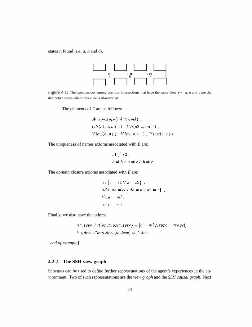
states it found (i.e.a, b andc).

a cb��������

����

��������

Figure 4.1:The agent moves among corridor intersections that have the same viewv+. a, b andc are the

distinctive states where this view is observed at.

The elements ofE are as follows:

Action type(ml; travel) ;

CS(s1; a;ml; b) ; CS(s2; b;ml; c) ;

V iew(a; v+) ; V iew(b; v+) ; V iew(c; v+) :

The uniqueness of names axioms associated withE are:

s1 6= s2 ;

a 6= b ^ a 6= c ^ b 6= c :

The domain closure axioms associated withE are:

8s fs = s1 _ s = s2g ;

8ds fds = a _ ds = b _ ds = cg ;

8a a = ml ;

8v v = v + :

Finally, we also have the axioms

8a; type Action type(a; type) � [a = ml ^ type = travel] ;

8a; desc Turn desc(a; desc) � false :

fend of exampleg

4.2.2 The SSH view graph

Schemas can be used to define further representations of the agent’s experiences in the en-vironment. Two of such representations are theview graphand theSSH causal graph. Next

24

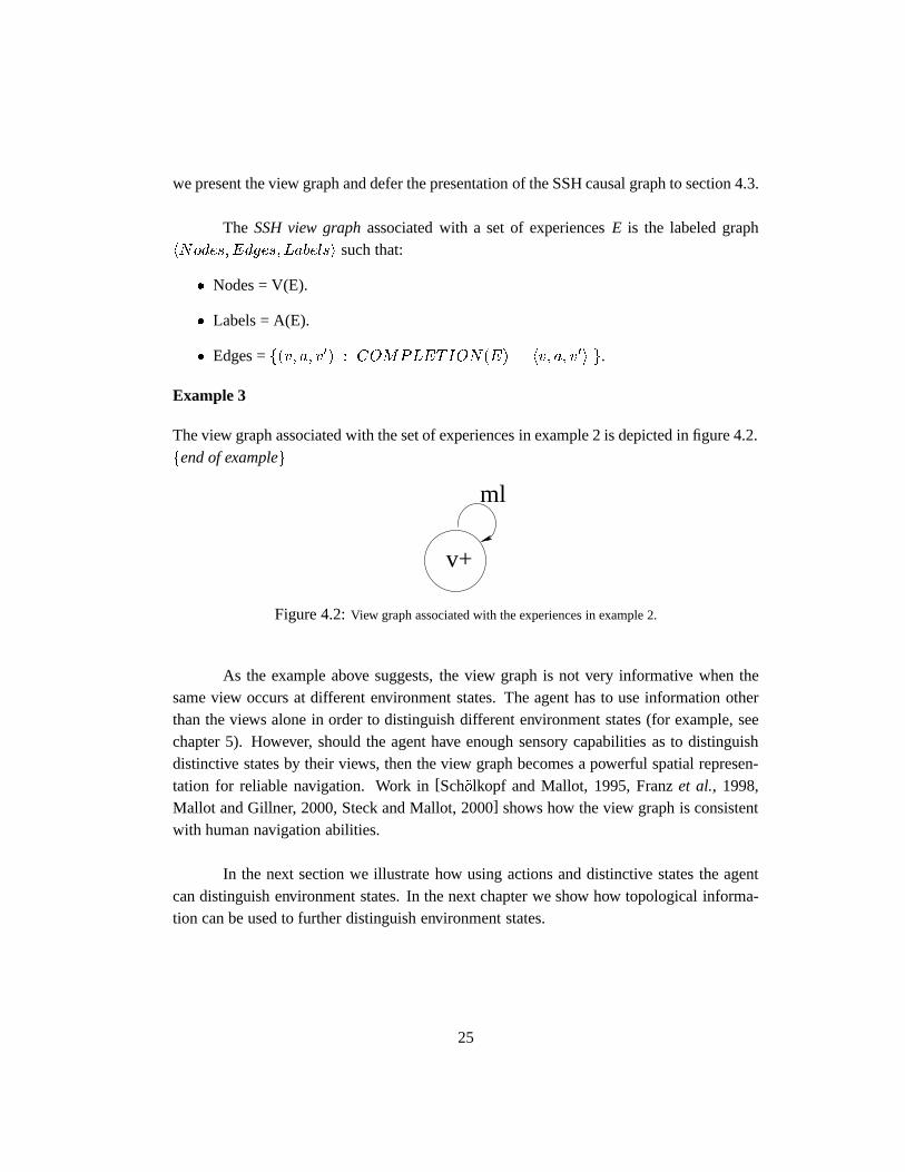
we present the view graph and defer the presentation of the SSH causal graph to section 4.3.

The SSH view graphassociated with a set of experiencesE is the labeled graphhNodes;Edges; Labelsi such that:

� Nodes = V(E).

� Labels = A(E).

� Edges =f(v; a; v0) : COMPLETION(E) j= hv; a; v0i g.

Example 3

The view graph associated with the set of experiences in example 2 is depicted in figure 4.2.fend of exampleg

ml

v+

Figure 4.2:View graph associated with the experiences in example 2.

As the example above suggests, the view graph is not very informative when thesame view occurs at different environment states. The agent has to use information otherthan the views alone in order to distinguish different environment states (for example, seechapter 5). However, should the agent have enough sensory capabilities as to distinguishdistinctive states by their views, then the view graph becomes a powerful spatial represen-tation for reliable navigation. Work in[Sch�olkopf and Mallot, 1995, Franzet al., 1998,Mallot and Gillner, 2000, Steck and Mallot, 2000] shows how the view graph is consistentwith human navigation abilities.

In the next section we illustrate how using actions and distinctive states the agentcan distinguish environment states. In the next chapter we show how topological informa-tion can be used to further distinguish environment states.

25

4.2.3 CT(E)

Given a set of experiencesE, the SSH causal theoryCT(E) defines when two distinctivestates are indistinguishable at the SSH causal level. We use the predicate

ceq(ds; ds0)

to denote the fact thatdistinctive statesds andds0 arecausallyindistinguishable.14 Infor-mally, ceq(ds; ds0) is the case whenever distinctive statesds andds0 are indistinguishableby the actions and views inE. We will assume that actions aredeterministic. Whenever theagent performs an action at a given distinctive state, it always ends up at the same distinctivestate:

hds; a; ds0i ^ hds; a; ds00i ! ds0 = ds00 : (4.22)

The SSH causal theory associated with a set of experiencesE, CT(E), is the follow-ing nested abnormality theory (NATs)[Lifschitz, 1995] (see appendix C, page 219):15

CT (E) = (4.23)

COMPLETION(E) ;

Axioms 4:1� 4:11 ;

hds; a; ds0i ^ hds; a; ds00i ! ds0 = ds00; (Axiom 4:22)

CEQ block

whereCEQ block is:

CEQ block =

f max ceq :

ceq(ds1; ds2)! ceq(ds2; ds1);

ceq(ds1; ds2) ^ ceq(ds2; ds3)! ceq(ds1; ds3);

ceq(ds1; ds2)! V iew(ds1; v) � V iew(ds2; v); (4.24)

ceq(ds1; ds2) ^ hds1; a; ds0

1i ^ hds2; a; ds0

2i ! ceq(ds01; ds0

2) (4.25)

g

Next we discuss the axioms definingceq. First at all, the predicateceq is an equiv-alence relation on the sort of distinctive states.

Theorem 1 The predicate ceq is an equivalence relation.14In chapter 5 we define when distinctive states are topologically indistinguishable.15Throughout this paper we assume that formulas are universally quantified.

26

Proof. See appendix E (page 229).16

Axiom 4.24 states that indistinguishable distinctive states have the same view. Fi-nally, axiom 4.25 states that if distinctive statesds andds0 are indistinguishable, then itshould be the case that if actiona has been performed for bothds andds0, the resultingdistinctive states should be indistinguishable. This axiom captures the following intuition:if ds andds0 are two indistinguishable distinctive states, any sequence of actions executedat ds andds0 will render the same sequence of views. Indeed, axioms 4.24 and 4.25 allowus to prove the following useful lemma:

Lemma 1 Let A denote a sequence of action symbols. LetA(ds) denote the distinctivestate symbol resulting from excuting the sequenceA starting at distinctive stateds, or? ifA is not defined fords.17 Then,

ceq(ds1; ds2) ^A(ds1) 6=? ^A(ds2) 6=?

! V iew(A(ds1); v) � V iew(A(ds2); v) :

There is a special case whenceq is an equivalence relation without writing theaxioms stating so. This happens when the result of every action at every distinctive state isknown. In this case, we say that the set of experiences iscomplete.

16Notice thatceq being reflexive does not follow fromceq being symmetric and transitive.17Given an action symbolA and distinctive stateds, A(ds) = ds0 if the schemahds;A; ds0i has been

observed, otherwise,A(ds) =?. Moreover,A(?) =?. The definition is then extended to action sequences inthe standard way. Notice thatA(ds) being well-defined relies on our assumption that actions are deterministic(axiom 4.22).

27

Definition 2

A set of experiencesE is completewhenever

E j= 8a; ds9ds0hds; a; ds0i :

fend of definitiong

Theorem 2 LetE be a complete set of experiences. LetCT(E)be defined as follows:

CT (E) =

COMPLETION(E) ;

Axioms 4:1� 4:11 ;

hds; a; ds0i ^ hds; a; ds00i ! ds0 = ds00; (Axiom 4:22)

CEQ block =

f max ceq :

ceq(ds1; ds2)! V iew(ds1; v) � V iew(ds2; v);

ceq(ds1; ds2) ^ h ds1; a; ds0

1 i ^ h ds2; a; ds0

2 i ! ceq(ds01; ds0

2)

g

Then the predicateceq is an equivalence relation.

Proof. See appendix E (page 232).

When a set of experiences is complete the predicateceqcaptures the idea that twodistinctive states are the same if they render the same views under any sequence of actions.Assume thatE is complete and letA = a1; : : : ; an denote a sequence of actions. SinceE

is complete,A(s) 6=? and the formulaV iew(A(ds); v) makes sense.

Theorem 3 LetE be a complete set of experiences. Then,

ceq(ds1; ds2) � 8A; v [V iew(A(ds1); v) � V iew(A(ds2); v)] :

Proof. See appendix E (page 234).

The problem of distinguishing environment states by outputs (views) and inputs(actions) has been studied in the framework of automata theory[Angluin, 1978, Gold, 1978,Rivest and Schapire, 1987, Basyeet al., 1995]. In this framework, the problem we addressis the one of finding the minimum automaton (w.r.t. the number of states) consistent with a

28

given set of input/output pairs. Without any particular assumptions about the environmentor the agent’s perceptual abilities, the problem of finding this smallest automaton is NP-complete ([Angluin, 1978, Gold, 1978]). The reader is referred to[Basyeet al., 1995] foran example of how to use automata to model dynamical systems.

Example 4

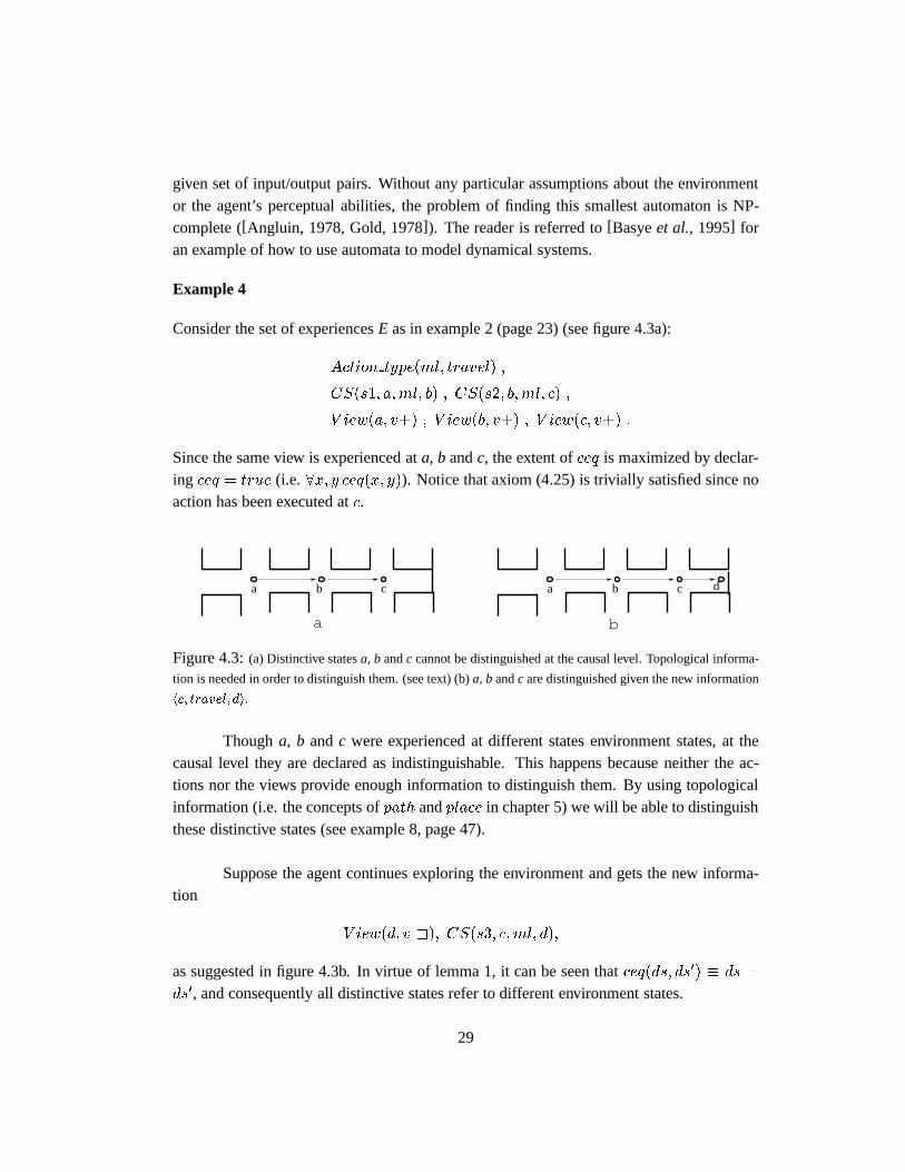
Consider the set of experiencesE as in example 2 (page 23) (see figure 4.3a):

Action type(ml; travel) ;

CS(s1; a;ml; b) ; CS(s2; b;ml; c) ;

V iew(a; v+) ; V iew(b; v+) ; V iew(c; v+) :

Since the same view is experienced ata, b andc, the extent ofceq is maximized by declar-ing ceq = true (i.e. 8x; y ceq(x; y)). Notice that axiom (4.25) is trivially satisfied since noaction has been executed atc.

a cb��������

����

��������

a b c d��������

����

��������

��������

a b

Figure 4.3:(a) Distinctive statesa, b andc cannot be distinguished at the causal level. Topological informa-

tion is needed in order to distinguish them. (see text) (b)a, b andc are distinguished given the new information

hc; travel; di.

Thougha, b andc were experienced at different states environment states, at thecausal level they are declared as indistinguishable. This happens because neither the ac-tions nor the views provide enough information to distinguish them. By using topologicalinformation (i.e. the concepts ofpath andplace in chapter 5) we will be able to distinguishthese distinctive states (see example 8, page 47).

Suppose the agent continues exploring the environment and gets the new informa-tion

V iew(d; v =); CS(s3; c;ml; d);

as suggested in figure 4.3b. In virtue of lemma 1, it can be seen thatceq(ds; ds0) � ds =

ds0, and consequently all distinctive states refer to different environment states.

29

fend of exampleg

As shown in the following example,there could exist different non-isomorphicmodels that maximize the extent of the predicateceq.

Example 5

LetE be the set defined by the following formulae:

Action type(ml; travel) ;

CS(s1; a;ml; b) ; CS(s2; c;ml; d) :

V iew(a; v) ; V iew(b; v) ; V iew(c; v) ; V iew(d; v1)

There are two different models forceq. In one of them,ceq(a; b) ^ :ceq(b; c) is the case,and in the other one:ceq(a; b) ^ ceq(b; c) is the case. Notice that in virtue of axiom 4.25,in both of these models:ceq(a; c) is the case.fend of exampleg

Different models ofCT (E) generally arise when the set of experiencesE is incom-plete (i.e. the agent has not completely explore the environment) or weak sensors inputs atdifferent environment states are classified as the same view.

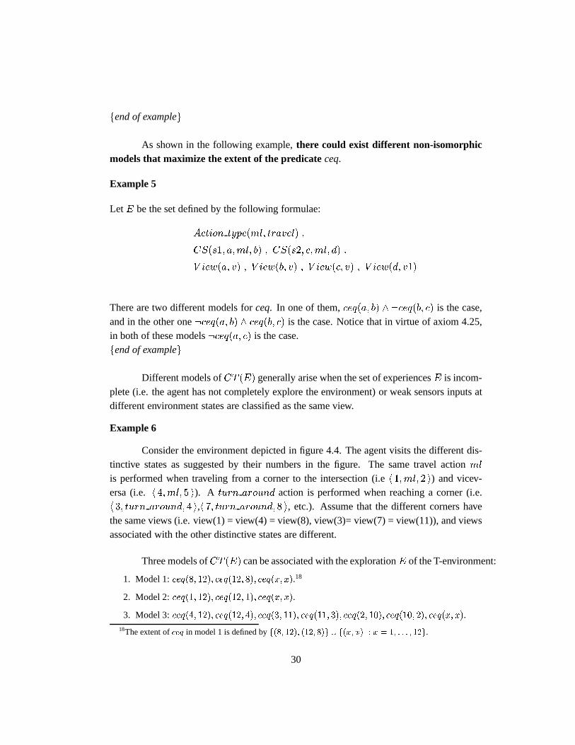
Example 6

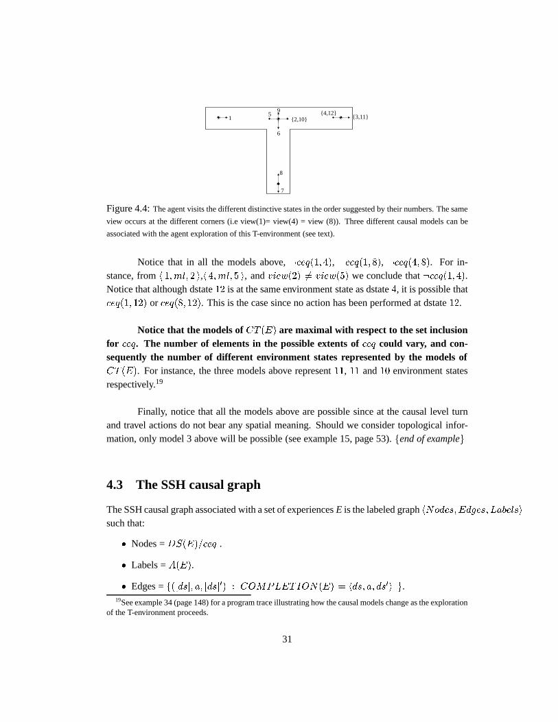
Consider the environment depicted in figure 4.4. The agent visits the different dis-tinctive states as suggested by their numbers in the figure. The same travel actionml

is performed when traveling from a corner to the intersection (i.eh 1;ml; 2 i) and vicev-ersa (i.e. h 4;ml; 5 i). A turn around action is performed when reaching a corner (i.e.h 3; turn around; 4 i,h 7; turn around; 8 i, etc.). Assume that the different corners havethe same views (i.e. view(1) = view(4) = view(8), view(3)= view(7) = view(11)), and viewsassociated with the other distinctive states are different.

Three models ofCT (E) can be associated with the explorationE of the T-environment:

1. Model 1:ceq(8; 12); ceq(12; 8); ceq(x; x).18

2. Model 2:ceq(1; 12); ceq(12; 1); ceq(x; x).

3. Model 3:ceq(4; 12); ceq(12; 4); ceq(3; 11); ceq(11; 3); ceq(2; 10); ceq(10; 2); ceq(x; x).

18The extent ofceq in model 1 is defined byf(8; 12); (12; 8)g [ f(x; x) : x = 1; : : : ; 12g.

30

��������

����

�� ��������

15

6

8

7

9

{2,10} {3,11}{4,12}

Figure 4.4:The agent visits the different distinctive states in the order suggested by their numbers. The same

view occurs at the different corners (i.e view(1)= view(4) = view (8)). Three different causal models can be

associated with the agent exploration of this T-environment (see text).

Notice that in all the models above,:ceq(1; 4), :ceq(1; 8), :ceq(4; 8). For in-stance, fromh 1;ml; 2 i,h 4;ml; 5 i, andview(2) 6= view(5) we conclude that:ceq(1; 4).Notice that although dstate12 is at the same environment state as dstate4, it is possible thatceq(1; 12) or ceq(8; 12). This is the case since no action has been performed at dstate12.

Notice that the models ofCT (E) are maximal with respect to the set inclusionfor ceq. The number of elements in the possible extents ofceq could vary, and con-sequently the number of different environment states represented by the models ofCT (E). For instance, the three models above represent11, 11 and10 environment statesrespectively.19

Finally, notice that all the models above are possible since at the causal level turnand travel actions do not bear any spatial meaning. Should we consider topological infor-mation, only model 3 above will be possible (see example 15, page 53).fend of exampleg

4.3 The SSH causal graph

The SSH causal graph associated with a set of experiencesE is the labeled graphhNodes;Edges; Labelsi

such that:

� Nodes =DS(E)=ceq .

� Labels =A(E).

� Edges =f([ds]; a; [ds]0) : COMPLETION(E) j= hds; a; ds0i g.19See example 34 (page 148) for a program trace illustrating how the causal models change as the exploration

of the T-environment proceeds.

31

whereDS(E)=ceq denotes the set of equivalence classes ofDS(E)moduloceq, and [ds]denotes the equivalence class ofds givenceq.

Example 7

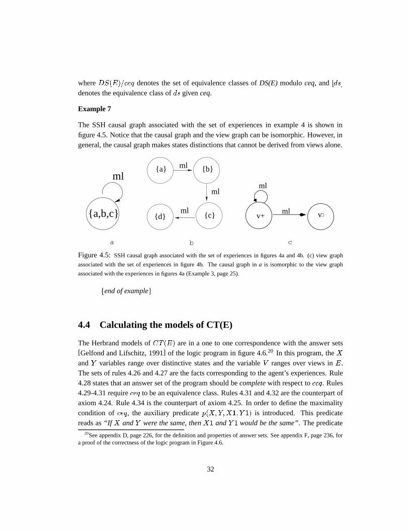
The SSH causal graph associated with the set of experiences in example 4 is shown infigure 4.5. Notice that the causal graph and the view graph can be isomorphic. However, ingeneral, the causal graph makes states distinctions that cannot be derived from views alone.

ml

{a,b,c} ml

ml

ml

{d} {c}

{b}{a}

ml

mlv+ v

a b c

Figure 4.5:SSH causal graph associated with the set of experiences in figures 4a and 4b. (c) view graph

associated with the set of experiences in figure 4b. The causal graph ina is isomorphic to the view graph

associated with the experiences in figures 4a (Example 3, page 25).

fend of exampleg

4.4 Calculating the models of CT(E)

The Herbrand models ofCT (E) are in a one to one correspondence with the answer sets[Gelfond and Lifschitz, 1991] of the logic program in figure 4.6.20 In this program, theXandY variables range over distinctive states and the variableV ranges over views inE.The sets of rules 4.26 and 4.27 are the facts corresponding to the agent’s experiences. Rule4.28 states that an answer set of the program should becompletewith respect toceq. Rules4.29-4.31 requireceq to be an equivalence class. Rules 4.31 and 4.32 are the counterpart ofaxiom 4.24. Rule 4.34 is the counterpart of axiom 4.25. In order to define the maximalitycondition of ceq, the auxiliary predicatep(X;Y;X1; Y 1) is introduced. This predicatereads as“If X andY were the same, thenX1 andY 1 would be the same”. The predicate

20See appendix D, page 226, for the definition and properties of answer sets. See appendix F, page 236, fora proof of the correctness of the logic program in Figure 4.6.

32

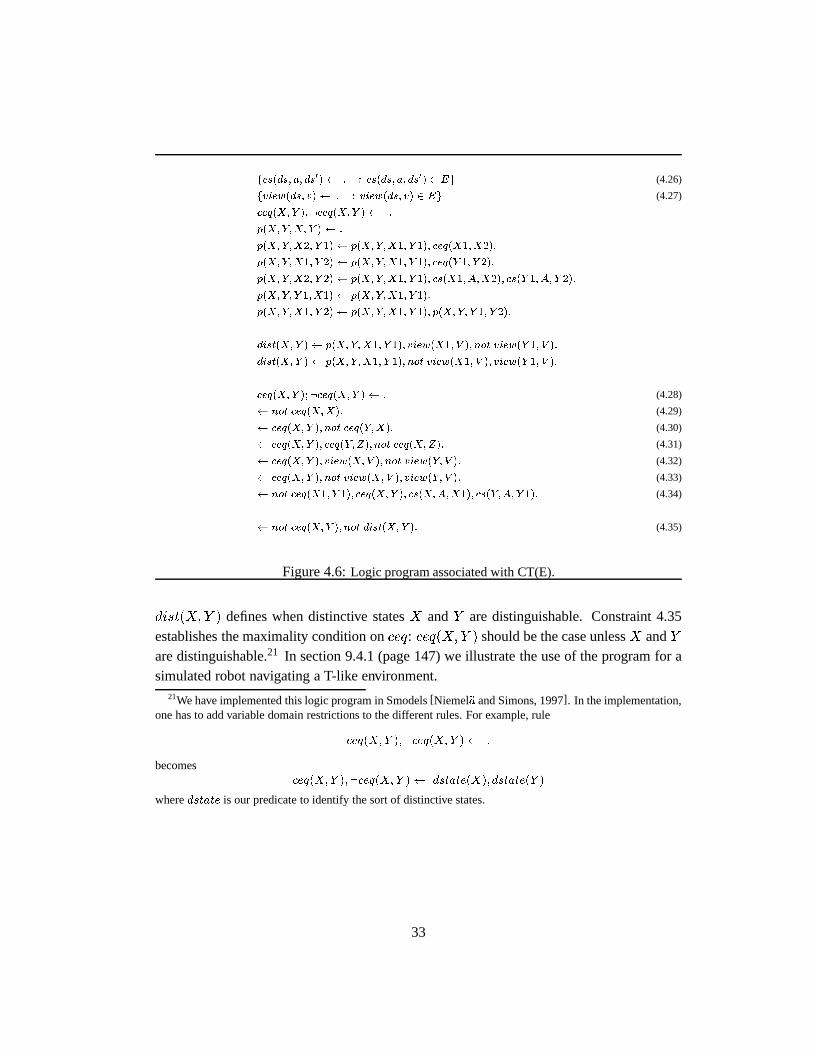
fcs(ds; a; ds0) : : cs(ds; a; ds0) 2 Eg (4.26)

fview(ds; v) : : view(ds; v) 2 Eg (4.27)

ceq(X; Y );:ceq(X;Y ) :

p(X; Y;X; Y ) :

p(X; Y;X2; Y 1) p(X;Y;X1; Y 1); ceq(X1;X2):

p(X; Y;X1; Y 2) p(X;Y;X1; Y 1); ceq(Y 1; Y 2):

p(X; Y;X2; Y 2) p(X;Y;X1; Y 1); cs(X1; A;X2); cs(Y 1; A; Y 2):

p(X; Y; Y 1;X1) p(X;Y;X1; Y 1):

p(X; Y;X1; Y 2) p(X;Y;X1; Y 1); p(X;Y; Y 1; Y 2):

dist(X; Y ) p(X;Y;X1; Y 1); view(X1; V ); not view(Y 1; V ):

dist(X; Y ) p(X;Y;X1; Y 1); not view(X1; V ); view(Y 1; V ):

ceq(X; Y );:ceq(X;Y ) : (4.28)

not ceq(X;X): (4.29)

ceq(X;Y ); not ceq(Y;X): (4.30)

ceq(X;Y ); ceq(Y;Z); not ceq(X;Z): (4.31)

ceq(X;Y ); view(X;V ); not view(Y; V ): (4.32)

ceq(X;Y ); not view(X;V ); view(Y; V ): (4.33)

not ceq(X1; Y 1); ceq(X;Y ); cs(X;A;X1); cs(Y;A; Y 1): (4.34)

not ceq(X;Y ); not dist(X; Y ): (4.35)

Figure 4.6:Logic program associated with CT(E).

dist(X;Y ) defines when distinctive statesX andY are distinguishable. Constraint 4.35establishes the maximality condition onceq: ceq(X;Y ) should be the case unlessX andYare distinguishable.21 In section 9.4.1 (page 147) we illustrate the use of the program for asimulated robot navigating a T-like environment.

21We have implemented this logic program in Smodels[Niemel�a and Simons, 1997]. In the implementation,one has to add variable domain restrictions to the different rules. For example, rule

ceq(X;Y );:ceq(X; Y ) :

becomesceq(X;Y );:ceq(X; Y ) dstate(X); dstate(Y )

wheredstate is our predicate to identify the sort of distinctive states.

33

4.5 Summary

SSH schemas summarize the continuous interactions of the agent in the environment. Thisis done by storing the initial and final distinctive states (and their corresponding views) forany action execution. Schemas can then later be used for directing the agent behavior, plan-ning, or distinguishing distinctive states sharing a same view.

By considering only the views associated with the initial and final distinctive statesof a schema, we defined theSSH view graph(section 4.2.2, page 24), which relates differ-ent views by actions linking them. When the agent can discern most distinctive states bytheir views, the view graph can be used for planning routes between different distinctivestates. The view graph representation is consistent with human navigation abilities[Mallotand Gillner, 2000, Steck and Mallot, 2000].

By considering actions as well as views, the agent can further distinguish distinc-tive states. Two distinctive states,ds andds0, are distinguishable, if there is a sequenceof actions that when executed atds renders a different sequence of views than when it isexecuted atds0. “Spatial properties” are not associated with actions when used to distin-guish distinctive states. This may prevent the agent from differentiating distinctive statesthat correspond to different environment states. In the next chapter we show how action’s“spatial properties” can be used to create a different ontology from the causal one - that ofplacesandpaths- which in turn can be used to further differentiate distinctive states.

In section 4.2.3 (page 26) we defined the predicateceq which is the case for dis-tinctive states that are not distinguishable by actions and views. We investigated whetherthe axioms definingceq (the CEQ block) were necessary and stated conditions underwhich they can be simplified (see appendix E, Page 229). We then defined theSSH causalgraph whose nodes are classes of distinctive states (classes w.r.tceq). This representa-tion is akin to the view graph although it imposes further refinement in the set of en-vironment states that are consistent with the agent experiences. The problem of iden-tifying the minimum set of distinctive states consistent with the agent’s experiences isequivalent to the one of identifying the minimum automata consistent with a set of in-put/output pairs. This problem turns out to be NP-complete when no special propertiesabout the actions, views, or the environment are assumed[Angluin, 1978, Gold, 1978,Basyeet al., 1995].

Finally, in section 4.4 we defined a logic program whose answer sets are in an one

34

to one correspondence with the models of the SSH causal theory. In appendix F we presenta proof of this claim.

35

Chapter 5

Topological Level

Relations among the distinctive states and trajectories defined by the control level, andamong their summaries as schemas at the causal level, are effectively described by thetopological network. At the SSH topological level the ontology consists ofplaces, pathsandregions, with connectivity and containment relations among them.

Roughly speaking, aplacecorresponds to a set of distinctive states linked by turnwith no travel actions. Similarly, apathcorresponds to a set of distinctive states linked bytravel with no turn actions (except forturn aroundactions). Places and paths are createdby abduction, positing the minimal set of places, paths, and regions required to explain theavailable observations (i.e. a set of schemas).

Grouping places intoregionsallows an agent to reason efficiently about its spatialknowledge. Regions themselves can be grouped to form new regions. In chapter 8, we willstudy how to formally include this hierarchy of regions in the SSH. In the next chapter wedefineboundary regionsassociated with paths. Informally, a path has associated three dis-joint regions: the set of places in the path, the set of places to the left of the path, and the setof places to the right of the path. Boundary regions allow the agent to distinguish distinctivestates, for two distinctive states can be considered different if they are in different boundaryregions (see example 23, page 84).

The construction of the topological map is usually described as an abduction pro-cess[Kuipers and Byun, 1988, Kuipers and Byun, 1991, Kuiperset al., 1993, Kuipers, 1996,Kuipers, 2000]. This abduction process is defined in procedural terms inspired by the cur-rent implementation of the SSH. In this chapter we define the circumscriptive theory asso-ciated with the SSH topological level. The models associated with this theory define the

36

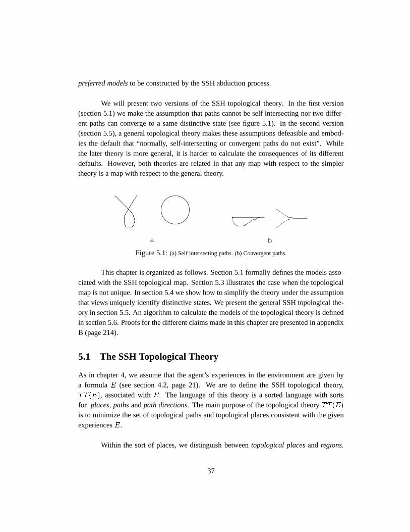
preferred modelsto be constructed by the SSH abduction process.

We will present two versions of the SSH topological theory. In the first version(section 5.1) we make the assumption that paths cannot be self intersecting nor two differ-ent paths can converge to a same distinctive state (see figure 5.1). In the second version(section 5.5), a general topological theory makes these assumptions defeasible and embod-ies the default that “normally, self-intersecting or convergent paths do not exist”. Whilethe later theory is more general, it is harder to calculate the consequences of its differentdefaults. However, both theories are related in that any map with respect to the simplertheory is a map with respect to the general theory.

a b

Figure 5.1:(a) Self intersecting paths. (b) Convergent paths.

This chapter is organized as follows. Section 5.1 formally defines the models asso-ciated with the SSH topological map. Section 5.3 illustrates the case when the topologicalmap is not unique. In section 5.4 we show how to simplify the theory under the assumptionthat views uniquely identify distinctive states. We present the general SSH topological the-ory in section 5.5. An algorithm to calculate the models of the topological theory is definedin section 5.6. Proofs for the different claims made in this chapter are presented in appendixB (page 214).

5.1 The SSH Topological Theory

As in chapter 4, we assume that the agent’s experiences in the environment are given bya formulaE (see section 4.2, page 21). We are to define the SSH topological theory,TT (E), associated withE. The language of this theory is a sorted language with sortsfor places, pathsandpath directions. The main purpose of the topological theoryTT (E)is to minimize the set of topological paths and topological places consistent with the givenexperiencesE.

Within the sort of places, we distinguish betweentopological placesand regions.

37

A topological place is a set of distinctive states linked by turn actions. A region is a set ofplaces. We use the predicatestpathandis region to identify these subsorts. A path definesan order relation among places connected by travel with no turn actions. They play the roleof streets in a city layout. Among paths,topological pathscorrespond to those paths whoseplaces are topological places. We use the predicatetpath to identify these paths. Otherpaths could exists whose places are regions. We use the predicateroute to identify thesepaths.

The distinctions between topological places and regions and between topologicalpaths and routes will allow the agent to learn from its own experiences as well as fromgiven information. For example, the agent could learn about places and paths by being told,or by “reading” a map. Our focus in this chapter is on describing the map learned fromactual experiences. We postpone the study of regions until chapters 6 and 8.

We require the sorts ofplaces and paths to be infinite. This is not to say thatthe SSH topological map has infinite number ofplaces or paths. As explained in sec-tion 5.3 (page 59), given a model of our theory, the SSH topological map corresponds tothe submodel obtained by restricting the different predicates totopological places, regions,topological pathsandroutes. Sincetopological placesare identified with set of distinctivestates andtopological pathsare identified with sequences of distinctive states, the topolog-ical map associated with a finite set of schemas (and so a finite set of distinctive states) hasa finite number oftopological placesand topological paths.1 Our requirement of infiniteplaces andpaths allow us to compare any two models of the theory. Example 22 (page 67)illustrates the use of this requirement.

A path has associated two directions,pos and neg. A path direction provides aframe of reference to establish the order in which places in a path are arranged or whether aplace is to the right or left of the path (see boundary regions in chapter 6). The sort of pathdirections is completely defined byposandneg:2

pos 6= neg ; (5.1)

8dir fdir = pos _ dir = negg : (5.2)

The language of the SSH topological level includes the following predicates:3

1. teq(ds,ds’): distinctive statesds andds0 aretopologically indistinguishable.1See proof in appendix B, theorem B, page 216.2For a directiondir,�dir is defined such that�pos = neg and�neg = pos.3Later we will make precise the informal meaning of these predicates.

38

2. tplace(p): placep is atopologicalplace.

3. is region(r): placer is aregion.

4. tpath(pa): pathpa is atopologicalpath.

5. route(pa): pathpa is aroute.

6. on(pa,p): placep is onpathpa.

7. order(pa,dir,p,q): placep is beforeplaceq, when facing directiondir on pathpa.

8. at(ds,p): distinctive stateds is atplacep.

9. along(ds,pa,dir): distinctive stateds is alongpathpa in directiondir.

The SSH topological theory associated withE, TT(E) , is the following nested ab-normality theory (NATs)[Lifschitz, 1995] (see appendix C, page 219):45

TT (E) = (5.3)

there exist infinitely many places ;

there exist infinitely many paths ;

:9p [tplace(p) ^ is region(p)] ; (5.4)

:9pa [tpath(pa) ^ route(pa)] ; (5.5)

Axioms 5:1� 5:2 ;

COMPLETION(E) ;

Axioms 4:1� 4:11 ;

hds; a; ds0i ^ hds; a; ds00i ! ds0 = ds00; (Axiom 4:22)

T block ;

f min is region; min route :

AT block

g

Axiom 5.4 says that topological places and regions are two subsorts of places. Sim-ilarly, axiom 5.5 says that topological paths and routes are two subsorts of paths. Theminimization criteria establishes that we are interested in models where the universe ofthese subsorts are as small as possible in order to explainE. Further requirements on paths

4A block of the form fC1; : : : ; Cn; minP1; : : : ;minPk : A1; : : : ; Amg denotes the set of blocksfC1; : : : ; Cn; minP1 : A1; : : : ; Amg, : : :, fC1; : : : ; Cn; minPk : A1; : : : ; Amg.

5The condition that the sorts of places and paths are infinite can be formalized requiring the existence of abijection between these sorts and the natural numbers.

39

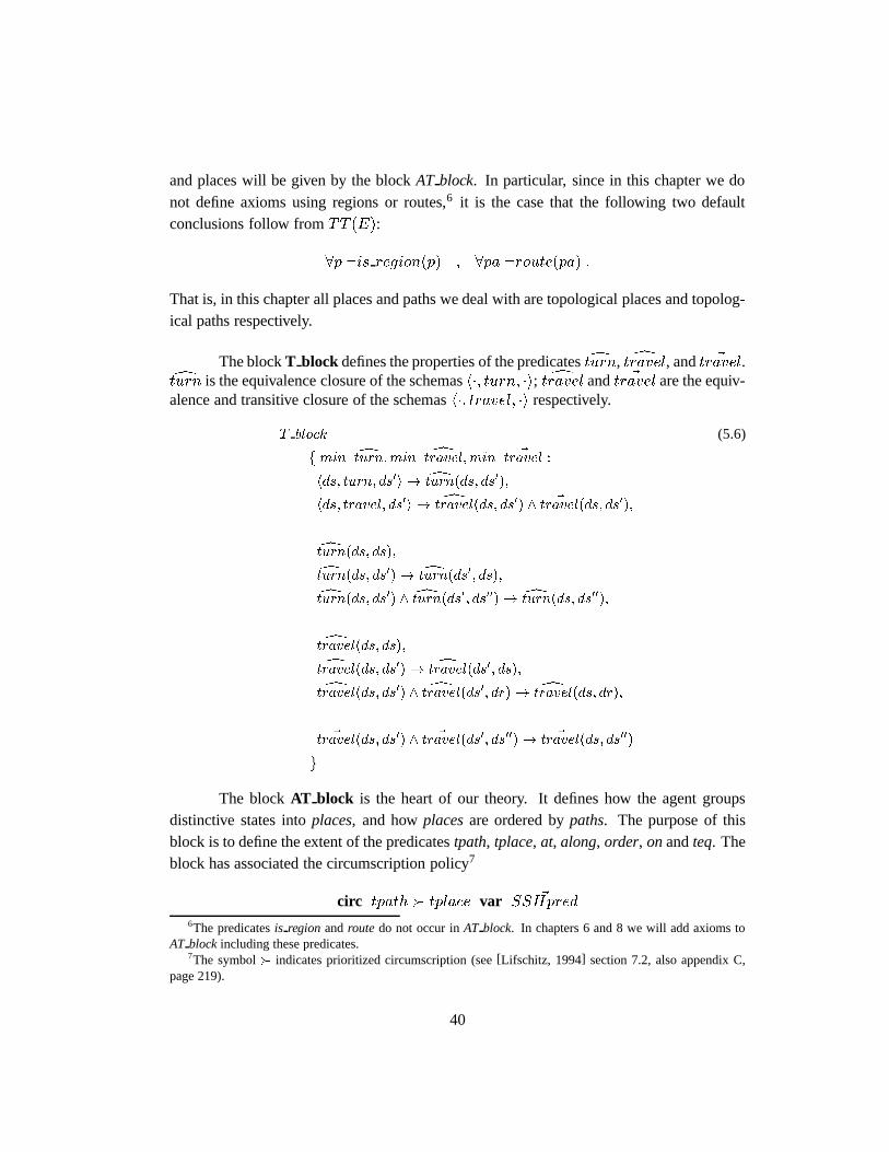
and places will be given by the blockAT block. In particular, since in this chapter we donot define axioms using regions or routes,6 it is the case that the following two defaultconclusions follow fromTT (E):

8p :is region(p) ; 8pa :route(pa) :

That is, in this chapter all places and paths we deal with are topological places and topolog-ical paths respectively.

The blockT block defines the properties of the predicatesdturn, dtravel, and ~travel.dturn is the equivalence closure of the schemash�; turn; �i; dtravel and ~travel are the equiv-alence and transitive closure of the schemash�; travel; �i respectively.

T block = (5.6)

f min dturn;min dtravel;min ~travel :

hds; turn; ds0i ! dturn(ds; ds0);hds; travel; ds0i ! dtravel(ds; ds0) ^ ~travel(ds; ds0);

dturn(ds; ds);dturn(ds; ds0)! dturn(ds0; ds);dturn(ds; ds0) ^ dturn(ds0; ds00)! dturn(ds; ds00);dtravel(ds; ds);dtravel(ds; ds0)! dtravel(ds0; ds);dtravel(ds; ds0) ^ dtravel(ds0; dr) ! dtravel(ds; dr);~travel(ds; ds0) ^ ~travel(ds0; ds00)! ~travel(ds; ds00)

g

The blockAT block is the heart of our theory. It defines how the agent groupsdistinctive states intoplaces, and howplacesare ordered bypaths. The purpose of thisblock is to define the extent of the predicatestpath, tplace, at, along, order, onandteq. Theblock has associated the circumscription policy7

circ tpath � tplace var ~SSHpred

6The predicatesis region androute do not occur inAT block. In chapters 6 and 8 we will add axioms toAT block including these predicates.

7The symbol� indicates prioritized circumscription (see[Lifschitz, 1994] section 7.2, also appendix C,page 219).

40

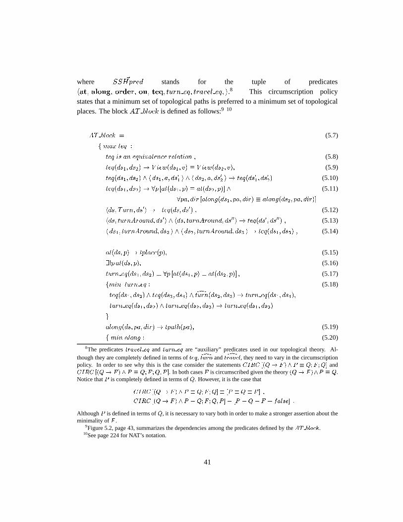
where ~SSHpred stands for the tuple of predicateshat; along; order; on; teq; turn eq; travel eq; i.8 This circumscription policystates that a minimum set of topological paths is preferred to a minimum set of topologicalplaces. The blockAT block is defined as follows:9 10

AT block = (5.7)

f max teq :

teq is an equivalence relation ; (5.8)

teq(ds1; ds2)! V iew(ds1; v) � V iew(ds2; v); (5.9)

teq(ds1; ds2) ^ h ds1; a; ds0

1 i ^ h ds2; a; ds0

2 i ! teq(ds01; ds0

2) (5.10)

teq(ds1; ds2)! 8p [at(ds1; p) � at(ds2; p)] ^ (5.11)

8pa; dir [along(ds1; pa; dir) � along(ds2; pa; dir)]

hds; Turn; ds0i ! :teq(ds; ds0) ; (5.12)

hds; turnAround; ds0i ^ hds; turnAround; ds00i ! teq(ds0; ds00) ; (5.13)

h ds1; turnAround; ds2 i ^ h ds2; turnAround; ds3 i ! teq(ds1; ds3) ; (5.14)

at(ds; p)! tplace(p); (5.15)

9!p at(ds; p); (5.16)

turn eq(ds1; ds2) � 8p [at(ds1; p) � at(ds2; p)] ; (5.17)

fmin turn eq : (5.18)

teq(ds1; ds2) ^ teq(ds3; ds4) ^ dturn(ds2; ds3)! turn eq(ds1; ds4);

turn eq(ds1; ds2) ^ turn eq(ds2; ds3)! turn eq(ds1; ds3)

g

along(ds; pa; dir)! tpath(pa); (5.19)

f min along : (5.20)

8The predicatestravel eq and turn eq are “auxiliary” predicates used in our topological theory. Al-though they are completely defined in terms ofteq, dturn and dtravel, they need to vary in the circumscriptionpolicy. In order to see why this is the case consider the statementsCIRC [(Q! F ) ^ P � Q;F ;Q] andCIRC [(Q! F ) ^ P � Q;F ;Q;P ]. In both casesF is circumscribed given the theory(Q! F )^P � Q.Notice thatP is completely defined in terms ofQ. However, it is the case that

CIRC [(Q! F ) ^ P � Q;F ;Q] � [P � Q � F ] ;

CIRC [(Q! F ) ^ P � Q;F ;Q;P ] � [P � Q � F � false] :

AlthoughP is defined in terms ofQ, it is necessary to vary both in order to make a stronger assertion about theminimality of F .

9Figure 5.2, page 43, summarizes the dependencies among the predicates defined by theAT block.10See page 224 for NAT’s notation.

41

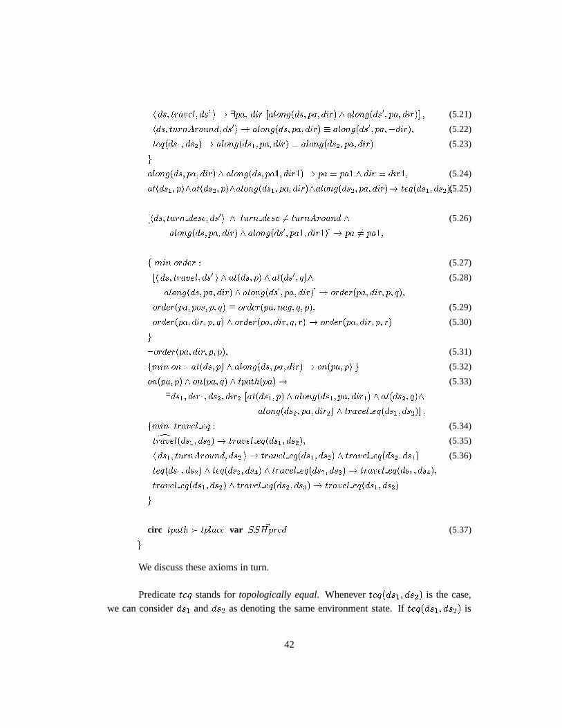
h ds; travel; ds0 i ! 9pa; dir [along(ds; pa; dir) ^ along(ds0; pa; dir)] ; (5.21)

hds; turnAround; ds0i ! along(ds; pa; dir) � along(ds0; pa;�dir); (5.22)

teq(ds1; ds2)! along(ds1; pa; dir) � along(ds2; pa; dir) (5.23)

g

along(ds; pa; dir) ^ along(ds; pa1; dir1)! pa = pa1 ^ dir = dir1; (5.24)

at(ds1; p)^at(ds2; p)^along(ds1; pa; dir)^along(ds2; pa; dir)! teq(ds1; ds2);(5.25)

[hds; turn desc; ds0i ^ turn desc 6= turnAround ^ (5.26)

along(ds; pa; dir) ^ along(ds0; pa1; dir1)]! pa 6= pa1;

f min order : (5.27)

[h ds; travel; ds0 i ^ at(ds; p) ^ at(ds0; q)^ (5.28)

along(ds; pa; dir) ^ along(ds0; pa; dir)]! order(pa; dir; p; q);

order(pa; pos; p; q) � order(pa; neg; q; p); (5.29)

order(pa; dir; p; q) ^ order(pa; dir; q; r) ! order(pa; dir; p; r) (5.30)

g

:order(pa; dir; p; p); (5.31)

fmin on : at(ds; p) ^ along(ds; pa; dir)! on(pa; p) g (5.32)

on(pa; p) ^ on(pa; q) ^ tpath(pa)! (5.33)

9ds1; dir1; ds2; dir2 [at(ds1; p) ^ along(ds1; pa; dir1) ^ at(ds2; q)^

along(ds2; pa; dir2) ^ travel eq(ds1; ds2)] ;

fmin travel eq : (5.34)dtravel(ds1; ds2)! travel eq(ds1; ds2); (5.35)

h ds1; turnAround; ds2 i ! travel eq(ds1; ds2) ^ travel eq(ds2; ds1) (5.36)

teq(ds1; ds2) ^ teq(ds3; ds4) ^ travel eq(ds2; ds3)! travel eq(ds1; ds4);

travel eq(ds1; ds2) ^ travel eq(ds2; ds3)! travel eq(ds1; ds3)

g

circ tpath � tplace var ~SSHpred (5.37)

g

We discuss these axioms in turn.

Predicateteq stands fortopologically equal. Wheneverteq(ds1; ds2) is the case,we can considerds1 andds2 as denoting the same environment state. Ifteq(ds1; ds2) is

42

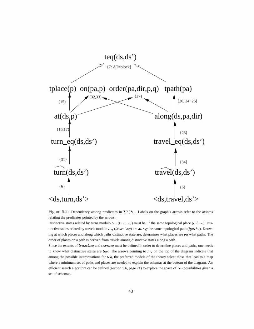
{31}

tplace(p) on(pa,p) order(pa,dir,p,q) tpath(pa)

turn(ds,ds’) travel(ds,ds’)

<ds,turn,ds’> <ds,travel,ds’>

turn_eq(ds,ds’) travel_eq(ds,ds’)

at(ds,p) along(ds,pa,dir)

teq(ds,ds’){7: AT=block}

{15}

{16,17}

{32,33} {27}{20, 24−26}

{23}

{34}

{6}{6}

Figure 5.2: Dependency among predicates inTT (E). Labels on the graph’s arrows refer to the axioms

relating the predicates pointed by the arrows.

Distinctive states related by turns moduloteq (turn eq) must beat the same topological place (tplace). Dis-

tinctive states related by travels moduloteq (travel eq) arealong the same topological path (tpaths). Know-

ing at which places and along which paths distinctive state are, determines what places areon what paths. The

order of places on a path is derived from travels among distinctive states along a path.

Since the extents oftravel eq andturn eq must be defined in order to determine places and paths, one needs

to know what distinctive states areteq. The arrows pointing toteq on the top of the diagram indicate that

among the possible interpretations forteq, the preferred models of the theory select those that lead to a map

where a minimum set of paths and places are needed to explain the schemas at the bottom of the diagram. An

efficient search algorithm can be defined (section 5.6, page 71) to explore the space ofteq possibilities given a

set of schemas.

43

the case,ds1 andds2 cannot be distinguished by views and actions (axioms 5.9 and 5.10),they are at the same place and along the same path direction.11

Axiom 5.12 states that aturn action takes the agent from one distinctive state toa different one. In particular we assume that a schema of the formhds; Turn; dsi is notincluded in the agent’s experiences. Axiom 5.13 states that there is a unique (moduloteq)distinctive state resulting from performing a turn around action. After two turn around ac-tions the agent is back to the same dstate (Axiom 5.14). Turn around actions are specialsince they link distinctive states along the same path but in opposite directions (axiom 5.22).

Axioms 5.16-5.17 state how the agent groups distinctive states into places. Everydistinctive state is at a unique topological place (axiom 5.16). Whenever the agentturns,it stays at the same topological place (axiom 5.17). Distinctive states grouped into a topo-logical place should beturn connected (moduloteq) (axiom 5.17).12

Travelactions among distinctive states are abstracted to topological paths connect-ing the places associated with such distinctive states (axioms 5.21 and 5.28). Travel ax-ioms are explained in terms of the two related predicates,along andorder. Both of thesepredicates are the minimum ones explaining travel actions and satisfying other propertiesincluded in their respective blocks 5.20 and 5.27.

Block 5.20 defines the predicatealong. Whenever an agentturns around, it staysin the same path but facing the opposite path’s direction (axiom 5.22). Axiom 5.23 is atrivial consequence of the definition ofteq but it needs to be included in the block so thatthe interpretation ofalong has tuples other than the ones explicitly derived from schemas(see example 10, page 49).

There are further restrictions on the properties ofalong. For instance, a distinctivestate is along at most one path (axiom 5.24). Since axiom 5.24 provides “negative” infor-mation aboutalong, it does not need to be included in block 5.20 (see proposition 4 in[Lifschitz, 1994]). Axiom 5.24 prevents the existence of different paths that converge to thesame distinctive state (see example 18, page 57). In section 5.5 we will make this axiom adefault.

11It is possible that the maximization ofteq in theAT block implies thatteq is an equivalence relationwithout explicitly requiring so. However at this point we do not have a proof for this claim.

12Block 5.18 states that the predicateturn eq corresponds to the relationdturn moduloteq.

44

Turn actions other thanturnAroundchange the path the initial and final distinctivestates linked by the action are along (axiom 5.26). This axiom allows the agent to concludethe existence of different paths once it turns right or left at a place (see Example 13, Page51). This axiom prevents the existence of self-intersecting paths as illustrated in figure 5.1.In section 5.5 we will make this axiom a default.

Block 5.27 defines the predicateorder. In addition to explaining travel actions,order defines an order among the places on a path satisfying the following two properties:i) the order of places in a given path direction is the inverse of the order of places in theother path direction (axiom 5.29), and ii), the order of places in a path is transitive (axiom5.30).

There are further restrictions on the properties oforder: i) the order of places ina path should be non-reflexive (axiom 5.31), and ii) the agent has to have traveled amongthe places on the same path (axiom 5.33). Since these requirements provide “negative” in-formation aboutorder, they do not need to be included in block 5.27 (see proposition 4 in[Lifschitz, 1994]). Notice that we rule out the existence of circular paths (axiom 5.31). Insection 5.5 we will make this axiom a default.

Axiom 5.33 requires the agent to have traveled among the places on a same path.travel eq defines when two distinctive states are linked by travel actions without turns(except forTurnAround actions) (see block 5.34). Example 14 illustrates how by usingtravel eq the agent can minimize the set of topological paths.

The SSH topological theoryTT (E) describes those places,tplaces, and paths,tpaths, that capture the intended meaning ofturn andtravel actions. This is done in sucha way that a minimum number of topological places and topological paths are identified.The blockAT block formally states this minimality criterion. A minimum set of topologi-cal paths is identified even at the cost of increasing the set of topological places. Figure 5.2shows the dependency among the different predicates inTT (E).

Remark. Axiom 5.24 implies a stronger version of axioms 5.21 and 5.28, namely:

at(ds; p) ^ at(ds0; q) ^ ~travel(ds; ds0)!

9!pa; dir [order(pa; dir; p; q) ^ along(ds; pa; dir) ^ along(ds0; pa; dir)] :

Using the above statement in combination with axiom 5.31 we deduce that whenever theagent has directly traveled between two distinctive states, the places associated with these

45

distinctive states are different:

~travel(ds; ds0) ^ at(ds; p) ^ at(ds0; q)! p 6= q

The statement above can be rewritten as

Corollary 1

~travel(ds; ds0)! place(ds) 6= place(ds0)

whereplace(ds) denotes the unique topological place that distinctive stateds is at (axiom5.16).

Moreover, consecutive travels among distinctive states occur along the same topo-logical path, as stated in the next corollary.

Corollary 2

n�1

i=1

~travel(dsi; dsi+1)!

9!pa; dir

"tpath(pa) ^

n

i=1

forder(pa; dir; place(dsi); place(dsi+1)) ^ along(dsi; pa; dir)g

#

While the sorts ofplaces and paths for a modelM of TT (E) are infinite, theinterpretation oftpath andtplace is finite. Indeed,

Theorem 4 The topological map associated with a finite set of experiencesE has a finitenumber of topological paths and a finite number of topological places.

Proof. See appendix B, page 216.2

Finally, it is important to note that our circumscription policy 5.37 and the fact thatthe sort of paths and places is infinite implies the following fact:13

Theorem 5 Any two models of the SSH topological theory have the same number of topo-logical paths and the same number of topological places.

Proof. See appendix B (page 216).2

However, theorem 5 does not mean that a unique map is associated with a set ofschemas. As shown in example 19 (page 59) the SSH topological theory could have more

13Recall that the interpretations fortpath andtplace are finite.

46

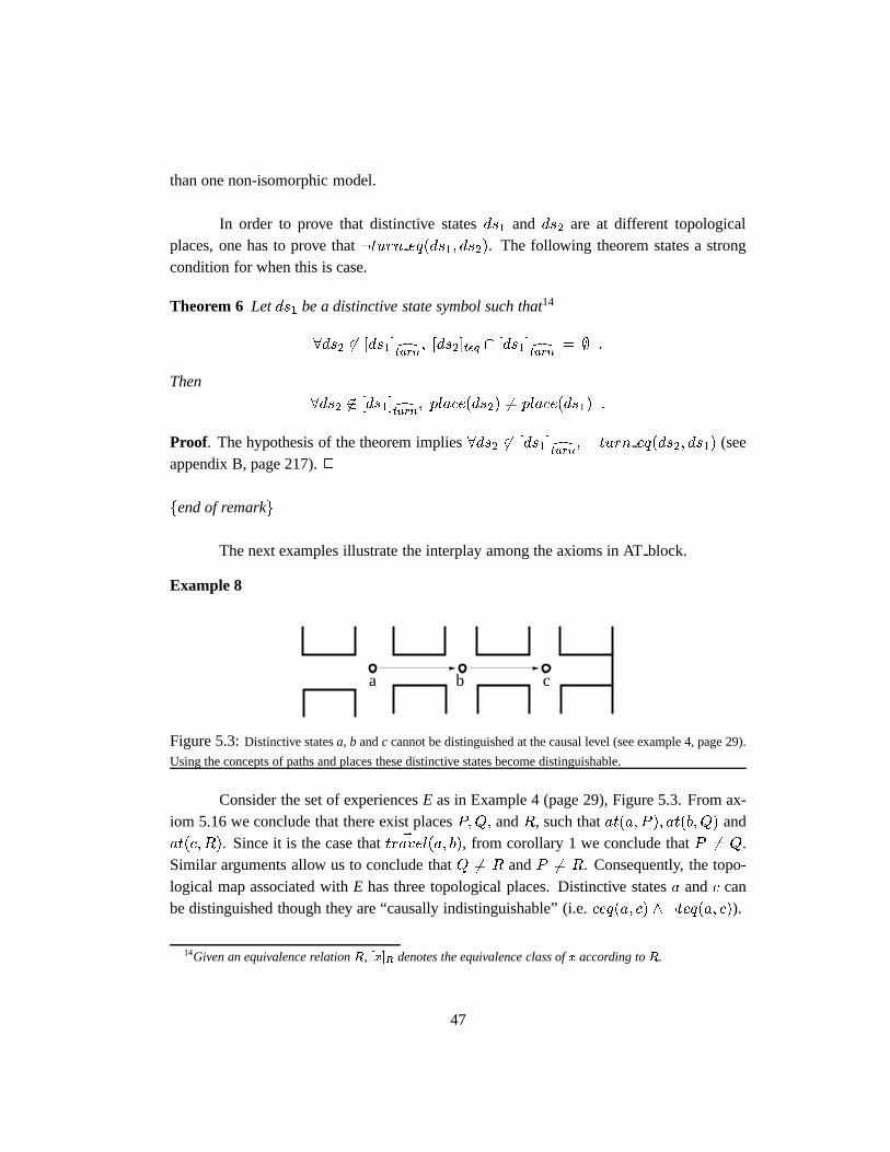
than one non-isomorphic model.

In order to prove that distinctive statesds1 and ds2 are at different topologicalplaces, one has to prove that:turn eq(ds1; ds2). The following theorem states a strongcondition for when this is case.

Theorem 6 Letds1 be a distinctive state symbol such that14

8ds2 62 [ds1]dturn; [ds2]teq \ [ds1]dturn = ; :

Then8ds2 62 [ds1]dturn; place(ds2) 6= place(ds1) :

Proof. The hypothesis of the theorem implies8ds2 62 [ds1]dturn; :turn eq(ds2; ds1) (seeappendix B, page 217).2

fend of remarkg

The next examples illustrate the interplay among the axioms in ATblock.

Example 8

a cb��������

����

��������

Figure 5.3:Distinctive statesa, b andc cannot be distinguished at the causal level (see example 4, page 29).

Using the concepts of paths and places these distinctive states become distinguishable.

Consider the set of experiencesE as in Example 4 (page 29), Figure 5.3. From ax-iom 5.16 we conclude that there exist placesP;Q; andR, such thatat(a; P ); at(b;Q) andat(c;R). Since it is the case that ~travel(a; b), from corollary 1 we conclude thatP 6= Q.Similar arguments allow us to conclude thatQ 6= R andP 6= R. Consequently, the topo-logical map associated withE has three topological places. Distinctive statesa andc canbe distinguished though they are “causally indistinguishable” (i.e.ceq(a; c) ^ :teq(a; c)).

14Given an equivalence relationR, [x]R denotes the equivalence class ofx according toR.

47

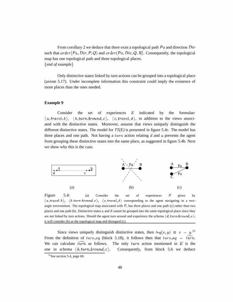
From corollary 2 we deduce that there exist a topological pathPa and directionDirsuch thatorder(Pa;Dir; P;Q) andorder(Pa;Dir;Q;R). Consequently, the topologicalmap has one topological path and three topological places.fend of exampleg

Only distinctive states linked by turn actions can be grouped into a topological place(axiom 5.17). Under incomplete information this constraint could imply the existence ofmore places than the ones needed.

Example 9

Consider the set of experiencesE indicated by the formulae:h a; travel; b i; h b; turnAround; c i; h c; travel; d i, in addition to the views associ-ated with the distinctive states. Moreover, assume that views uniquely distinguish thedifferent distinctive states. The model forTT(E) is presented in figure 5.4c. The model hasthree places and one path. Not having aturn action relatingd anda prevents the agentfrom grouping these distinctive states into the same place, as suggested in figure 5.4b. Nextwe show why this is the case.

����

���� �

��

���

���

���

������

������

������

������

������

������

(a) (b) (c)

CPa

BPaABPaAb

ca

d

Figure 5.4: (a) Consider the set of experiences E given by

h a; travel; b i; h b; turnAround; c i; h c; travel; d i corresponding to the agent navigating in a rect-

angle environment. The topological map associated withE, has three places and one path (c) rather than two

places and one path (b). Distinctive statesa andd cannot be grouped into the same topological place since they

are not linked by turn actions. Should the agent turn around and experience the schemah d; turnAround; a i,

it will consider (b) as the topological map and disregard (c).

Since views uniquely distinguish distinctive states, thenteq(x; y) � x = y.15

From the definition ofturn eq (block 5.18), it follows then thatturn eq = dturn.We can calculatedturn as follows. The onlyturn action mentioned inE is theone in schemah b; turnAround; c i. Consequently, from block 5.6 we deduce

15See section 5.4, page 60.

48

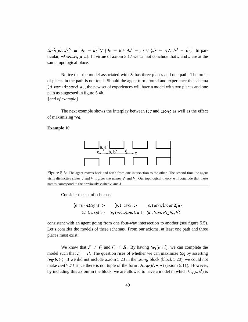
dturn(ds; ds0) � [ds = ds0 _ fds = b ^ ds0 = cg _ fds = c ^ ds0 = bg]. In par-ticular,:turn eq(a; d). In virtue of axiom 5.17 we cannot conclude thata andd are at thesame topological place.

Notice that the model associated withE has three places and one path. The orderof places in the path is not total. Should the agent turn around and experience the schemah d; turnAround; a i, the new set of experiences will have a model with two places and onepath as suggested in figure 5.4b.fend of exampleg

The next example shows the interplay betweenteq andalong as well as the effectof maximizingteq.

Example 10

e d ca, a’

b, b’

Figure 5.5:The agent moves back and forth from one intersection to the other. The second time the agent

visits distinctive statesa andb, it gives the namesa0 andb0. Our topological theory will conclude that these

names correspond to the previously visiteda andb.

Consider the set of schemas

ha; turnRight; bi hb; travel; ci hc; turnAround; di

hd; travel; ei he; turnRight; a0i ha0; turnRight; b0i

consistent with an agent going from one four-way intersection to another (see figure 5.5).Let’s consider the models of these schemas. From our axioms, at least one path and threeplaces must exist:

We know thatP 6= Q andQ 6= R. By having teq(a; a0), we can complete themodel such thatP = R. The question rises of whether we can maximizeteq by assertingteq(b; b0). If we did not include axiom 5.23 in thealong block (block 5.20), we could notmaketeq(b; b0) since there is not tuple of the formalong(b0; �; �) (axiom 5.11). However,by including this axiom in the block, we are allowed to have a model in whichteq(b; b0) is

49

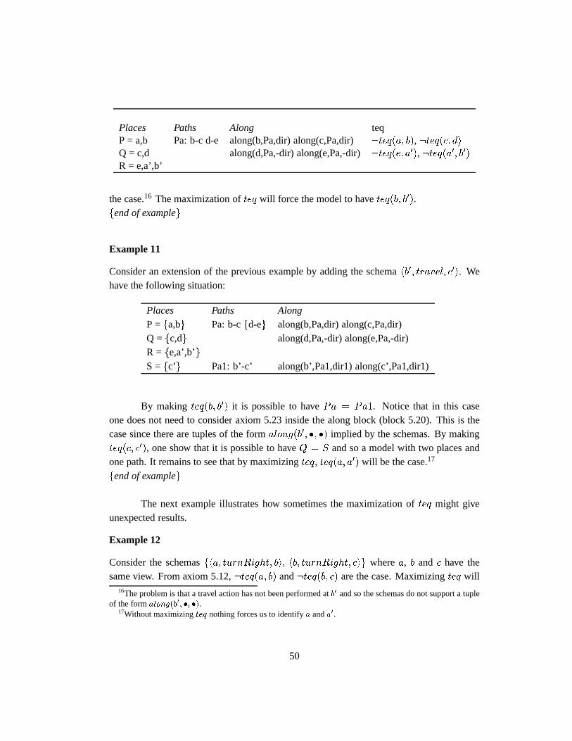
Places Paths Along teqP = a,b Pa: b-c d-e along(b,Pa,dir) along(c,Pa,dir):teq(a; b), :teq(c; d)Q = c,d along(d,Pa,-dir) along(e,Pa,-dir):teq(e; a0), :teq(a0; b0)R = e,a’,b’

the case.16 The maximization ofteq will force the model to haveteq(b; b0).fend of exampleg

Example 11

Consider an extension of the previous example by adding the schemahb0; travel; c0i. Wehave the following situation:

Places Paths AlongP =fa,bg Pa: b-cfd-eg along(b,Pa,dir) along(c,Pa,dir)Q = fc,dg along(d,Pa,-dir) along(e,Pa,-dir)R = fe,a’,b’gS =fc’g Pa1: b’-c’ along(b’,Pa1,dir1) along(c’,Pa1,dir1)

By making teq(b; b0) it is possible to havePa = Pa1. Notice that in this caseone does not need to consider axiom 5.23 inside the along block (block 5.20). This is thecase since there are tuples of the formalong(b0; �; �) implied by the schemas. By makingteq(c; c0), one show that it is possible to haveQ = S and so a model with two places andone path. It remains to see that by maximizingteq, teq(a; a0) will be the case.17

fend of exampleg

The next example illustrates how sometimes the maximization ofteq might giveunexpected results.

Example 12

Consider the schemasfha; turnRight; bi; hb; turnRight; cig wherea, b and c have thesame view. From axiom 5.12,:teq(a; b) and:teq(b; c) are the case. Maximizingteq will

16The problem is that a travel action has not been performed atb0 and so the schemas do not support a tupleof the formalong(b0; �; �).

17Without maximizingteq nothing forces us to identifya anda0.

50

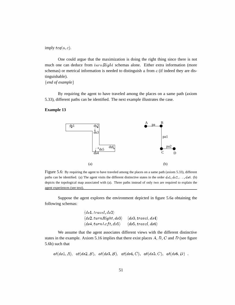
imply teq(a; c).

One could argue that the maximization is doing the right thing since there is notmuch one can deduce fromturnRight schemas alone. Either extra information (moreschemas) or metrical information is needed to distinguisha from c (if indeed they are dis-tinguishable).fend of exampleg

By requiring the agent to have traveled among the places on a same path (axiom5.33), different paths can be identified. The next example illustrates the case.

Example 13

(a) (b)

D

pa2

C

pa1

BpaA

ds3

ds1

ds4

ds2

ds6ds5

Figure 5.6:By requiring the agent to have traveled among the places on a same path (axiom 5.33), different

paths can be identified. (a) The agent visits the different distinctive states in the orderds1; ds2; : : : ; ds6. (b)

depicts the topological map associated with (a). Three paths instead of only two are required to explain the

agent experiences (see text).

Suppose the agent explores the environment depicted in figure 5.6a obtaining thefollowing schemas:

hds1; travel; ds2i

hds2; turnRight; ds3i hds3; travel; ds4i

hds4; turnLeft; ds5i hds5; travel; ds6i

We assume that the agent associates different views with the different distinctivestates in the example. Axiom 5.16 implies that there exist placesA,B,C andD (see figure5.6b) such that

at(ds1; A); at(ds2; B); at(ds3; B); at(ds4; C); at(ds5; C); at(ds6;D) :

51

Moreover, corollary 1 implies that

A 6= B ; B 6= C ; C 6= D :

Under our assumption that all distinctive states in the example have different views, it fol-lows then thatteq(ds1; ds2) � ds1 = ds2 and thus dturn = turn eq (see section 5.4).Since:dturn(ds1; ds3), :dturn(ds1; d5) and:dturn(ds2; ds6) are the case, it follows that

A 6= C; A 6= D; B 6= D :

Consequently, placesA, B, C andD are all different.

Axiom 5.21 implies that there exist pathsPa; Pa1; Pa2, and directionsdir; dir1; dir2, such that:

order(Pa; dir;A;B); along(ds1; Pa; dir); along(ds2; Pa; dir);

order(Pa1; dir1; B;C); along(ds3; Pa1; dir1); along(ds4; Pa1; dir1);

order(Pa2; dir2; C;D); along(ds5; Pa2; dir2); along(ds6; Pa2; dir2) :

Since we have the schemashds2; turnRight; ds3i andhds4; turnLeft; ds5i, axiom 5.26implies that

Pa 6= Pa1; Pa1 6= Pa2 :

Since teq(ds1; ds2) � ds1 = ds2 and there is notturnAround schemas inE, thendtravel = travel eq. Consequently: dtravel(ds1; ds4) and: dtravel(ds1; ds5) are the case,and in virtue of axiom 5.33 it follows that

Pa 6= Pa2 :

fend of exampleg

Next we illustrate how the predicatetravel eq is used when defining topologicalpaths.

Example 14

Consider the environment in figure 5.7. Suppose the agent starts at distinctive statea andvisits places A,B,C,D,E, and F as suggested by the arrows in the figure.18 The correspond-ing set of experiences contains the formulaeV iew(a; va), V iew(b; vb), ha; travel; bi, etc..

18A capital letterL denotes the topological place associated with distinctive statel.

52

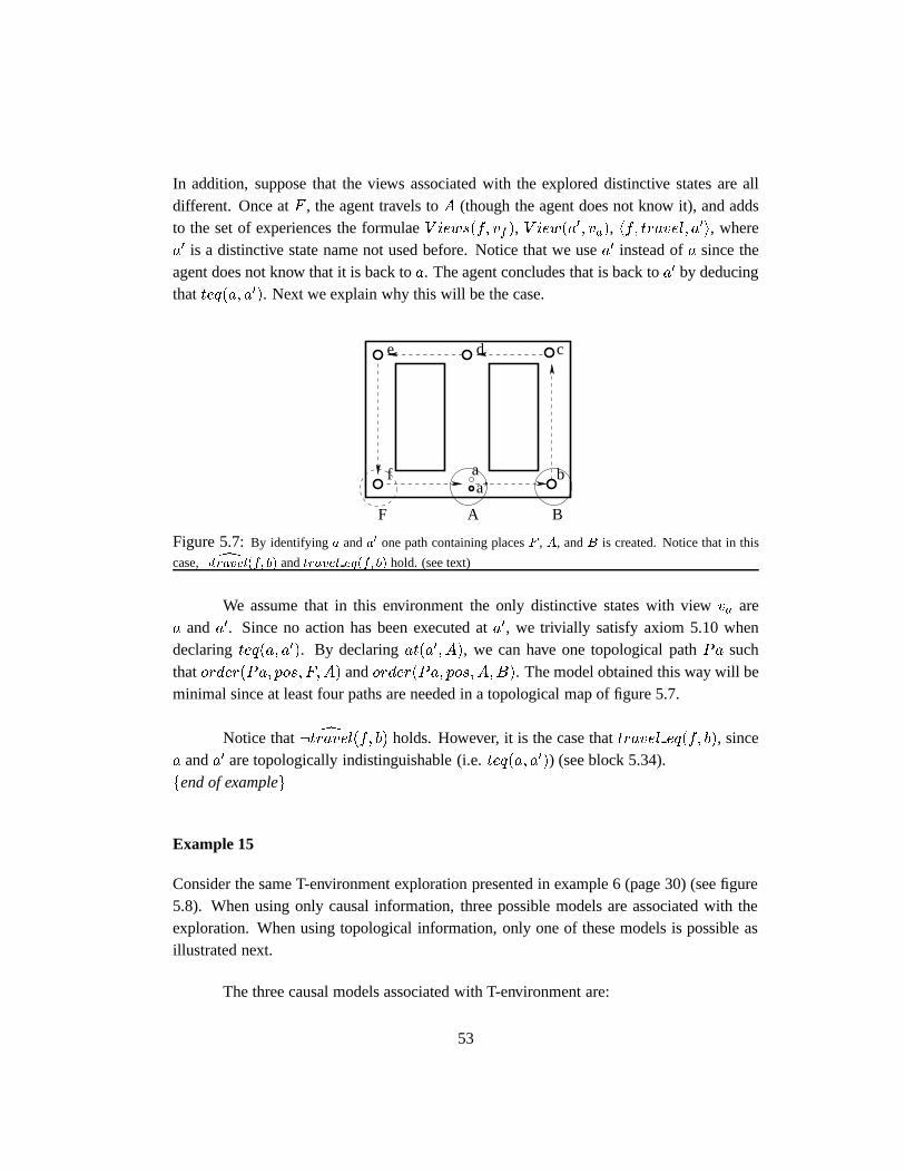
In addition, suppose that the views associated with the explored distinctive states are alldifferent. Once atF , the agent travels toA (though the agent does not know it), and addsto the set of experiences the formulaeV iews(f; vf ), V iew(a0; va), hf; travel; a0i, wherea0 is a distinctive state name not used before. Notice that we usea0 instead ofa since theagent does not know that it is back toa. The agent concludes that is back toa0 by deducingthatteq(a; a0). Next we explain why this will be the case.

F A B

fa’

ba

de c

Figure 5.7:By identifying a anda0 one path containing placesF , A, andB is created. Notice that in this

case,: dtravel(f; b) andtravel eq(f; b) hold. (see text)

We assume that in this environment the only distinctive states with viewva area anda0. Since no action has been executed ata0, we trivially satisfy axiom 5.10 whendeclaringteq(a; a0). By declaringat(a0; A), we can have one topological pathPa suchthatorder(Pa; pos; F;A) andorder(Pa; pos;A;B). The model obtained this way will beminimal since at least four paths are needed in a topological map of figure 5.7.

Notice that: dtravel(f; b) holds. However, it is the case thattravel eq(f; b), sincea anda0 are topologically indistinguishable (i.e.teq(a; a0)) (see block 5.34).fend of exampleg

Example 15

Consider the same T-environment exploration presented in example 6 (page 30) (see figure5.8). When using only causal information, three possible models are associated with theexploration. When using topological information, only one of these models is possible asillustrated next.

The three causal models associated with T-environment are:

53

��������

����

�� ��������

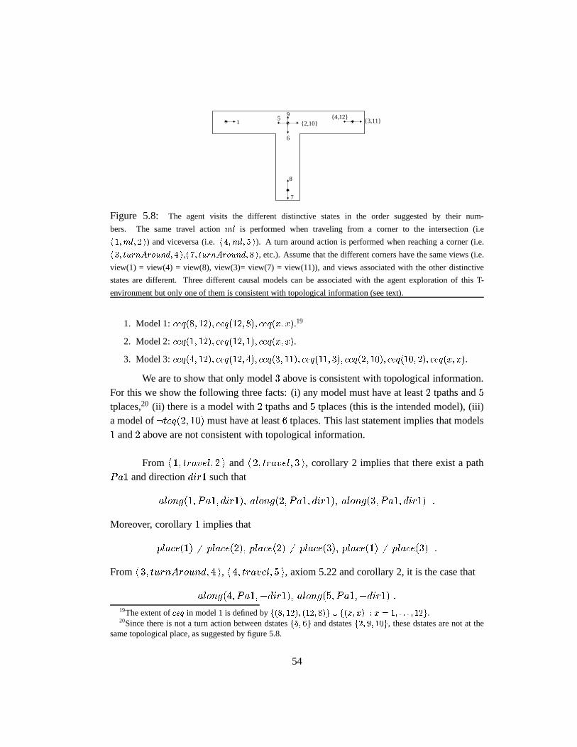
15

6

8

7

9

{2,10} {3,11}{4,12}

Figure 5.8: The agent visits the different distinctive states in the order suggested by their num-

bers. The same travel actionml is performed when traveling from a corner to the intersection (i.e

h 1;ml; 2 i) and viceversa (i.e.h 4;ml; 5 i). A turn around action is performed when reaching a corner (i.e.

h 3; turnAround; 4 i,h 7; turnAround; 8 i, etc.). Assume that the different corners have the same views (i.e.

view(1) = view(4) = view(8), view(3)= view(7) = view(11)), and views associated with the other distinctive

states are different. Three different causal models can be associated with the agent exploration of this T-

environment but only one of them is consistent with topological information (see text).

1. Model 1:ceq(8; 12); ceq(12; 8); ceq(x; x).19

2. Model 2:ceq(1; 12); ceq(12; 1); ceq(x; x).

3. Model 3:ceq(4; 12); ceq(12; 4); ceq(3; 11); ceq(11; 3); ceq(2; 10); ceq(10; 2); ceq(x; x).

We are to show that only model3 above is consistent with topological information.For this we show the following three facts: (i) any model must have at least2 tpaths and5tplaces,20 (ii) there is a model with2 tpaths and5 tplaces (this is the intended model), (iii)a model of:teq(2; 10) must have at least6 tplaces. This last statement implies that models1 and2 above are not consistent with topological information.

From h 1; travel; 2 i andh 2; travel; 3 i, corollary 2 implies that there exist a pathPa1 and directiondir1 such that

along(1; Pa1; dir1); along(2; Pa1; dir1); along(3; Pa1; dir1) :

Moreover, corollary 1 implies that

place(1) 6= place(2); place(2) 6= place(3); place(1) 6= place(3) :

Fromh 3; turnAround; 4 i, h 4; travel; 5 i, axiom 5.22 and corollary 2, it is the case that

along(4; Pa1;�dir1); along(5; Pa1;�dir1) :19The extent ofceq in model 1 is defined byf(8; 12); (12; 8)g [ f(x; x) : x = 1; : : : ; 12g.20Since there is not a turn action between dstatesf5; 6g and dstatesf2; 9; 10g, these dstates are not at the

same topological place, as suggested by figure 5.8.

54

Similarly, from h 5; turnLeft; 6 i, h 6; travel; 7 i, h 7; turnAround; 8 i, h 8; travel; 9 i weconclude that there exist a pathPa2 and directiondir2 such thatPa1 6= Pa2 (axiom 5.26)and

place(5) 6= place(8); along(6; Pa2; dir2); along(7; Pa2; dir2);

along(8; Pa2;�dir2); along(9; Pa2;�dir2) :

Fromh 9; turnRight; 10 i, h 10; travel; 11 i, h 11; turnAround; 12 i, there exist pathPa3and directiondir3 such thatPa2 6= Pa3 and

along(10; Pa3; dir3); along(11; Pa3; dir3); along(12; Pa3;�dir3) :

Theorem 6 allow us to conclude thatplace(5) 62 fplace(1); place(2); place(3)g. The sameargument shows thatplace(8) 62 fplace(1); place(2); place(3); place(5)g. Consequently,a miminal model of the theory must have at least two tpaths and five tplaces.

Notice that in the intended model of the T-environment,Pa1 = Pa3, dir1 = dir3,teq(2; 10), teq(3; 11) andteq(4; 12). This model is indeed a model ofTT (E) since at leasttwo topological paths and five topological places are needed to explainE, and consequentlyany model must have two topological paths and five topological places (theorem 5).

If :teq(2; 10) were the case, then theorem 6 allows to conclude thatplace(9) 62

fplace(1); place(2); place(3); place(5); place(8)g and so the model will have at least sixtplaces. Consequentlyteq(2; 10) has to be the case in a minimal model of the theory.fend of exampleg

Example 16

Consider an extension of the previous example where we have the additional schemas

h 9; turnLeft; 50 i; h 50; turnRight; 9 i :

In this case, the intended model hasfour places and two paths. Notice that now the agentcan conclude thatplace(5) = place(2) by makingteq(50; 5) and soturn eq(5; 2). fend ofexampleg

Our theory does not assume that paths intersect at most in one place. Consider thenext example.

Example 17

55

����

��������

��������

������������

������������

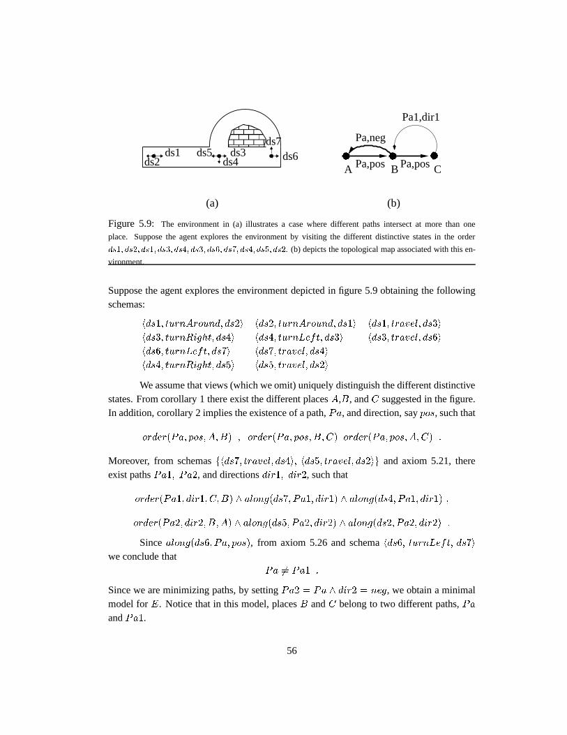
ds1ds2 ds4

ds3 ds6

Pa,neg

Pa1,dir1

CBPa,posA

(b)(a)

Pa,pos

ds7ds5

Figure 5.9: The environment in (a) illustrates a case where different paths intersect at more than one

place. Suppose the agent explores the environment by visiting the different distinctive states in the order

ds1; ds2; ds1; ds3; ds4; ds3; ds6; ds7; ds4; ds5; ds2. (b) depicts the topological map associated with this en-

vironment.

Suppose the agent explores the environment depicted in figure 5.9 obtaining the followingschemas:

hds1; turnAround; ds2i hds2; turnAround; ds1i hds1; travel; ds3i

hds3; turnRight; ds4i hds4; turnLeft; ds3i hds3; travel; ds6i

hds6; turnLeft; ds7i hds7; travel; ds4i

hds4; turnRight; ds5i hds5; travel; ds2i

We assume that views (which we omit) uniquely distinguish the different distinctivestates. From corollary 1 there exist the different placesA,B, andC suggested in the figure.In addition, corollary 2 implies the existence of a path,Pa, and direction, saypos, such that

order(Pa; pos;A;B) ; order(Pa; pos;B;C) order(Pa; pos;A;C) :

Moreover, from schemasfhds7; travel; ds4i; hds5; travel; ds2ig and axiom 5.21, thereexist pathsPa1; Pa2, and directionsdir1; dir2, such that

order(Pa1; dir1; C;B) ^ along(ds7; Pa1; dir1) ^ along(ds4; Pa1; dir1) ;

order(Pa2; dir2; B;A) ^ along(ds5; Pa2; dir2) ^ along(ds2; Pa2; dir2) :

Sincealong(ds6; Pa; pos), from axiom 5.26 and schemahds6; turnLeft; ds7iwe conclude that

Pa 6= Pa1 :

Since we are minimizing paths, by settingPa2 = Pa ^ dir2 = neg, we obtain a minimalmodel forE. Notice that in this model, placesB andC belong to two different paths,PaandPa1.

56

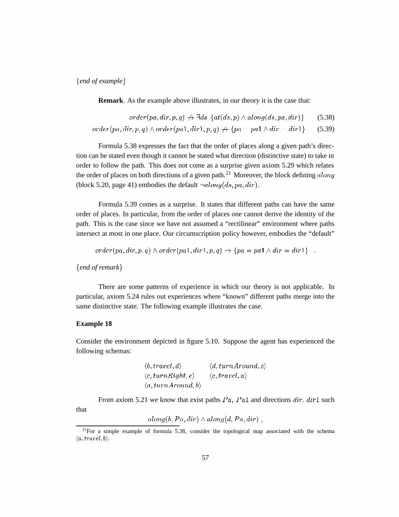
fend of exampleg

Remark. As the example above illustrates, in our theory it is the case that:

order(pa; dir; p; q) 6! 9ds fat(ds; p) ^ along(ds; pa; dir)g (5.38)

order(pa; dir; p; q) ^ order(pa1; dir1; p; q) 6! fpa = pa1 ^ dir = dir1g (5.39)

Formula 5.38 expresses the fact that the order of places along a given path’s direc-tion can be stated even though it cannot be stated what direction (distinctive state) to take inorder to follow the path. This does not come as a surprise given axiom 5.29 which relatesthe order of places on both directions of a given path.21 Moreover, the block definingalong(block 5.20, page 41) embodies the default:along(ds; pa; dir).

Formula 5.39 comes as a surprise. It states that different paths can have the sameorder of places. In particular, from the order of places one cannot derive the identity of thepath. This is the case since we have not assumed a “rectilinear” environment where pathsintersect at most in one place. Our circumscription policy however, embodies the “default”

order(pa; dir; p; q) ^ order(pa1; dir1; p; q)! fpa = pa1 ^ dir = dir1g :

fend of remarkg

There are some patterns of experience in which our theory is not applicable. Inparticular, axiom 5.24 rules out experiences where “known” different paths merge into thesame distinctive state. The following example illustrates the case.

Example 18

Consider the environment depicted in figure 5.10. Suppose the agent has experienced thefollowing schemas:

hb; travel; di hd; turnAround; ci

hc; turnRight; ei he; travel; ai

ha; turnAround; bi

From axiom 5.21 we know that exist pathsPa; Pa1 and directionsdir; dir1 suchthat

along(b; Pa; dir) ^ along(d; Pa; dir) ;

21For a simple example of formula 5.38, consider the topological map associated with the schemaha; travel; bi.

57

a b d

e

c

Figure 5.10:Distinctive statea is along two different paths, which contradicts axiom 5.24. Experiences like

the one in the figure are handled by the SSH general topological theory described in section 5.5.

along(e; Pa1; dir1) ^ along(a; Pa1; dir1) :

Moreover, from axiom 5.22 it follows that

along(b; Pa1;�dir1) :

From axiom 5.24 we conclude thatPa = Pa1. However, from schemahc; turnRight; eiand axiom 5.26 we conclude thatPa 6= Pa1 which is a contradiction.fend of exampleg

The previous example illustrates plausible patterns of experience that realistic envi-ronments could generate. In section 5.5 we extend our theory to cope with convergent pathslike the ones in the previous example.

5.2 teq versusceq

It is worth noticing thatteq satisfies the same axioms inside theCEQ block.22 Conse-quently, given an interpretation forteq it could be extended to at least one interpretation forceq. However, the converse it not true. Given an interpretation forceq it does not necessar-ily have a subset that defines an interpretation forteq. For instance, in example 15 (page53) only one of the three possible interpretations forceq admits a topological structure.

It is tempting to include an axiom liketeq(ds1; ds2)! ceq(ds1; ds2) in the defini-tion of teq (theAT block 5.7, page 41). However this will yield the wrong results sinceceq

is not varied in the block definingteq. In particular, theorem 5 will not be the case (will notbe a theorem!!), and model 2 in example 15 will admit a topological map with two tpathsand six tplaces.

22Compare axioms 5.9-5.10 (page 41) in the definition ofteq with axiom 4.24-4.25 inceq’s definition (page26.

58

5.3 The SSH topological map

Given a minimal modelM of TT (E), the SSH topological map is defined by the extent inM of tpath, tplace, along, order, on, at andteq. Notice that axioms 5.15 and 5.19 restrictthe domain ofat andalong to topological places and topological paths. The domain oforder is implicitly restricted to topological paths in virtue of block 5.27 and axiom 5.21.

While the sorts ofplaces and paths for a modelM of TT (E) are infinite, theinterpretation oftpath andtplaces is finite. Indeed,

Theorem 4The topological map associated with a finite set of experiencesE has afinite number of topological paths and a finite number of topological places.

Proof. See appendix B, page 216.2

Since the positive and negative direction of a path are chosen arbitrarily (Axiom5.21), there is not a unique minimal model forTT (E). Given any modelM of TT (E) onecould define another modelM 0 of TT (E) by choosing a pathpa in M and reversing theroles of the directionspos andneg for pa:

� orderM0

(Pa; pos;A;B) wheneverorderM(Pa; neg;A;B).23

� orderM0

(Pa; neg;A;B) wheneverorderM (Pa; pos;A;B).

� alongM0

(ds; Pa; pos) wheneveralongM (ds; Pa; neg).

� alongM0

(ds; Pa; neg) wheneveralongM (ds; Pa; pos).

� M 0 andM are equal otherwise.

We will consider these “up to path direction isomorphic” models to be the same.However, it is still the case that the theoryTT (E) has minimal models that are not isomor-phic up to path direction. In general, when distinctive states look alike (i.e. have the sameview), the agent’s experiences might not be enough to distinguish them. The next exampleillustrates this case.

Example 1923orderM

0

(Pa; pos; A;B) stands for the tuple(Pa; pos; A;B) belonging to the interpretation oforder inthe modelM 0.

59

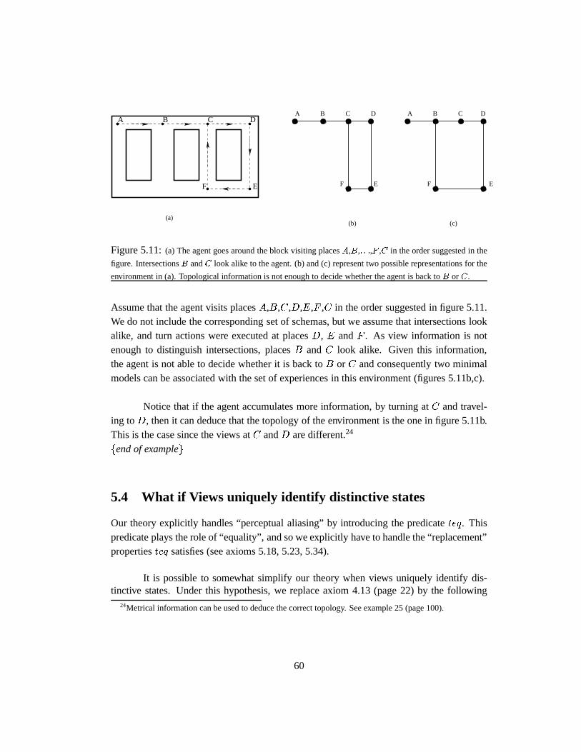
EF

B C DAA C D

EF

A C

(a)(b) (c)

B B D

EF

Figure 5.11:(a) The agent goes around the block visiting placesA,B,: : :,F ,C in the order suggested in the

figure. IntersectionsB andC look alike to the agent. (b) and (c) represent two possible representations for the

environment in (a). Topological information is not enough to decide whether the agent is back toB orC.

Assume that the agent visits placesA,B,C,D,E,F ,C in the order suggested in figure 5.11.We do not include the corresponding set of schemas, but we assume that intersections lookalike, and turn actions were executed at placesD, E andF . As view information is notenough to distinguish intersections, placesB andC look alike. Given this information,the agent is not able to decide whether it is back toB or C and consequently two minimalmodels can be associated with the set of experiences in this environment (figures 5.11b,c).

Notice that if the agent accumulates more information, by turning atC and travel-ing toD, then it can deduce that the topology of the environment is the one in figure 5.11b.This is the case since the views atC andD are different.24

fend of exampleg

5.4 What if Views uniquely identify distinctive states

Our theory explicitly handles “perceptual aliasing” by introducing the predicateteq. Thispredicate plays the role of “equality”, and so we explicitly have to handle the “replacement”propertiesteq satisfies (see axioms 5.18, 5.23, 5.34).

It is possible to somewhat simplify our theory when views uniquely identify dis-tinctive states. Under this hypothesis, we replace axiom 4.13 (page 22) by the following

24Metrical information can be used to deduce the correct topology. See example 25 (page 100).

60

axiom:

V iew(ds1; V ) ^ V iew(ds2; V )! ds1 = ds2 (5.40)

In virtue of axioms 4.24 and 5.9,ceq �= and teq �=, and beingceq and teqequivalence relations we conclude that they can be replaced by equality. The fact thatceq

andteq reduce to= is expected since all that is required to identify a distinctive state is itsview.

By replacingteq by =, block 5.18 can be rewritten as:

f min turn eq :dturn(ds2; ds3) ^ teq(ds1; ds2) ^ teq(ds3; ds4)! turn eq(ds1; ds4)

turn eq(ds1; ds2) ^ turn eq(ds2; ds3)! turn eq(ds1; ds3)

g

�

f min turn eq :dturn(ds2; ds3) ^ ds1 = ds2 ^ ds3 = ds4 ! turn eq(ds1; ds4)

turn eq(ds1; ds2) ^ turn eq(ds2; ds3)! turn eq(ds1; ds3)

g

�

f min turn eq :dturn(ds1; ds2)! turn eq(ds1; ds2)

turn eq(ds1; ds2) ^ turn eq(ds2; ds3)! turn eq(ds1; ds3)

g

� dturn = turn eq

where the last equality follows from the fact thatdturn is transitive, andturn eq is theminimum transitive predicate containingdturn. Consequently, we do not need the predicateturn eq in our formalization.

As for travel eq we can do some simplifications:

f min travel eq :dtravel(ds1; ds2)! travel eq(ds1; ds2);

h ds1; TurnAround; ds2 i ! travel eq(ds1; ds2) ^ travel eq(ds2; ds1)

teq(ds1; ds2) ^ teq(ds3; ds4) ^ travel eq(ds2; ds3)! travel eq(ds1; ds4);

travel eq(ds1; ds2) ^ travel eq(ds2; ds3)! travel eq(ds1; ds3)

61

g

�

f min travel eq :dtravel(ds1; ds2)! travel eq(ds1; ds2);

h ds1; TurnAround; ds2 i ! travel eq(ds1; ds2) ^ travel eq(ds2; ds1)

travel eq(ds1; ds2) ^ travel eq(ds2; ds3)! travel eq(ds1; ds3)

g

Therefore, if views uniquely identify distinctive states,AT block can be rewrittenas follows:

AT block =

f :

hds; turn; ds0i ! ds 6= ds0;

hds; turnAround; ds0i ^ hds; TurnAround; ds00i ! ds0 = ds00;

h ds1; turnAround; ds2 i ^ h ds2; turnAround; ds3 i ! ds1 = ds3 ;

at(ds; p)! tplace(p);

9!p at(ds; p);dturn(ds1; ds2) � 8p [at(ds1; p) � at(ds2; p)] ;

along(ds; pa; dir)! tpath(pa);

f min along :

h ds; travel; ds0 i ! 9pa; dir [along(ds; pa; dir) ^ along(ds0; pa; dir)] ;

hds; turnAround; ds0i ! along(ds; pa; dir) � along(ds0; pa;�dir);

g

along(ds; pa; dir) ^ along(ds; pa1; dir1)! pa = pa1 ^ dir = dir1;

at(ds1; p) ^ at(ds2; p) ^ along(ds1; pa; dir) ^ along(ds2; pa; dir)! ds1 = ds2;

[hds; turn desc; ds0i ^ turn desc 6= turnAround^

along(ds; pa; dir) ^ along(ds0; pa1; dir1)]! pa 6= pa1;

f min order :

[h ds; travel; ds0 i ^ at(ds; p) ^ at(ds0; q)^

along(ds; pa; dir) ^ along(ds0; pa; dir)]! order(pa; dir; p; q);

order(pa; pos; p; q) � order(pa; neg; q; p);

62

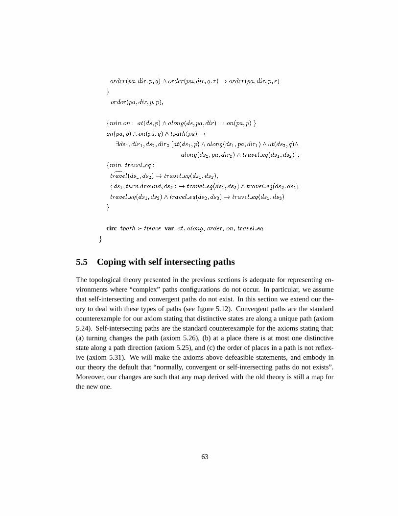
order(pa; dir; p; q) ^ order(pa; dir; q; r) ! order(pa; dir; p; r)

g

:order(pa; dir; p; p);

fmin on : at(ds; p) ^ along(ds; pa; dir)! on(pa; p) g

on(pa; p) ^ on(pa; q) ^ tpath(pa)!

9ds1; dir1; ds2; dir2 [at(ds1; p) ^ along(ds1; pa; dir1) ^ at(ds2; q)^

along(ds2; pa; dir2) ^ travel eq(ds1; ds2)] ;

fmin travel eq :dtravel(ds1; ds2)! travel eq(ds1; ds2);

h ds1; turnAround; ds2 i ! travel eq(ds1; ds2) ^ travel eq(ds2; ds1)

travel eq(ds1; ds2) ^ travel eq(ds2; ds3)! travel eq(ds1; ds3)

g

circ tpath � tplace var at; along; order; on; travel eq

g

5.5 Coping with self intersecting paths

The topological theory presented in the previous sections is adequate for representing en-vironments where “complex” paths configurations do not occur. In particular, we assumethat self-intersecting and convergent paths do not exist. In this section we extend our the-ory to deal with these types of paths (see figure 5.12). Convergent paths are the standardcounterexample for our axiom stating that distinctive states are along a unique path (axiom5.24). Self-intersecting paths are the standard counterexample for the axioms stating that:(a) turning changes the path (axiom 5.26), (b) at a place there is at most one distinctivestate along a path direction (axiom 5.25), and (c) the order of places in a path is not reflex-ive (axiom 5.31). We will make the axioms above defeasible statements, and embody inour theory the default that “normally, convergent or self-intersecting paths do not exists”.Moreover, our changes are such that any map derived with the old theory is still a map forthe new one.

63

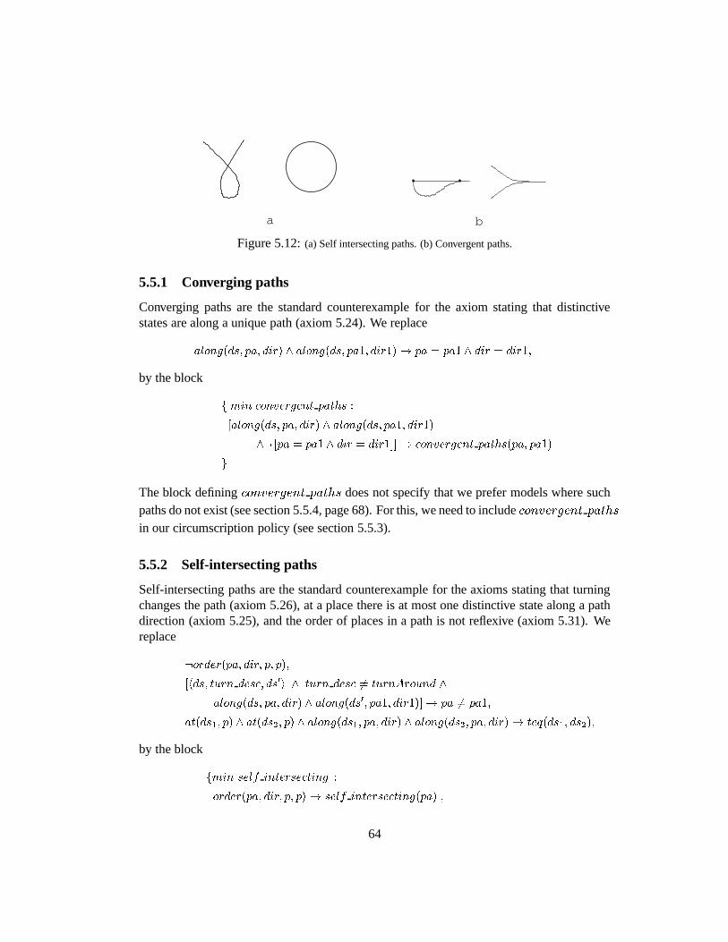
a b

Figure 5.12:(a) Self intersecting paths. (b) Convergent paths.

5.5.1 Converging paths

Converging paths are the standard counterexample for the axiom stating that distinctivestates are along a unique path (axiom 5.24). We replace

along(ds; pa; dir) ^ along(ds; pa1; dir1)! pa = pa1 ^ dir = dir1;

by the block

f min convergent paths :

[along(ds; pa; dir) ^ along(ds; pa1; dir1)

^: [pa = pa1 ^ dir = dir1]]! convergent paths(pa; pa1)

g

The block definingconvergent paths does not specify that we prefer models where suchpaths do not exist (see section 5.5.4, page 68). For this, we need to includeconvergent paths

in our circumscription policy (see section 5.5.3).

5.5.2 Self-intersecting paths

Self-intersecting paths are the standard counterexample for the axioms stating that turningchanges the path (axiom 5.26), at a place there is at most one distinctive state along a pathdirection (axiom 5.25), and the order of places in a path is not reflexive (axiom 5.31). Wereplace

:order(pa; dir; p; p);

[hds; turn desc; ds0i ^ turn desc 6= turnAround ^

along(ds; pa; dir) ^ along(ds0; pa1; dir1)]! pa 6= pa1;

at(ds1; p) ^ at(ds2; p) ^ along(ds1; pa; dir) ^ along(ds2; pa; dir)! teq(ds1; ds2);

by the block

fmin self intersecting :

order(pa; dir; p; p)! self intersecting(pa) ;

64

[hds; turn desc; ds0i ^ turn desc 6= TurnAround ^ along(ds; pa; dir)

^along(ds0; pa; dir1)]! self intersecting(pa) ;

[at(ds1; p) ^ at(ds2; p) ^ along(ds1; pa; dir) ^ along(ds2; pa; dir)

^:teq(ds1; ds2)]! self intersecting(pa)

g

Like convergent paths, the block definingself intersecting does not specify that we pre-fer models where such paths do not exist (see Section 5.5.4, page 68). For this, we need toincludeself intersecting in our circumscription policy (see section 5.5.3).

5.5.3 New circumscription policy

While we have defined convergent and self-intersecting paths, we still need to formalizethat by default these kind of paths do not exist. This is accomplished by giving priority tothe minimization of these two predicates over any other predicate. The new circumscriptionpolicy associated with our theory becomes

circ self intersecting � convergent paths � tpath � tplace var ~SSHpred: (5.41)

The intuition behind the predicate’s order in the circumscription is as follows: clearly ax-ioms 5.26 and 5.25 are about distinguishing paths, and so we need to minimizeself intersecting

even at the expense of having more topological paths.25 Example 20 illustrates why we givepriority toself intersecting overconvergent paths. As for the orderconvergent paths �tpath � tplace, we want to guarantee that maps according to the old theory are still mapsaccording to the new theory. In this sense, the new theory is a “conservative” extension ofour previous theory, as stated in the following theorem:

Theorem 7 Any topological map with respect to our previous theory is a topological mapaccording to the new theory.

25Notice that axiom 5.25 can be rewritten as follows:

at(ds1; p) ^ at(ds2; p) ^ along(ds1; pa; dir) ^ along(ds2; pa; dir)! teq(ds1; ds2)

� at(ds1; p) ^ at(ds2; p) ^ along(ds1; pa; dir) ^ along(ds2; pa1; dir) ^ pa = pa1! teq(ds1; ds2)

� at(ds1; p) ^ at(ds2; p) ^ along(ds1; pa; dir) ^ along(ds2; pa1; dir) ^ :teq(ds1; ds2)! pa 6= pa1

We beg the issue that axiom 5.31 is more about distinguishing places than it is about distinguishing paths. Infact

:order(pa; dir; p; p) � : [order(pa; dir; p; q) ^ p = q] � [order(pa; dir; p; q)! p 6= q] :

At the very least we need to haveself intersecting � tplace in the circumscription policy.

65

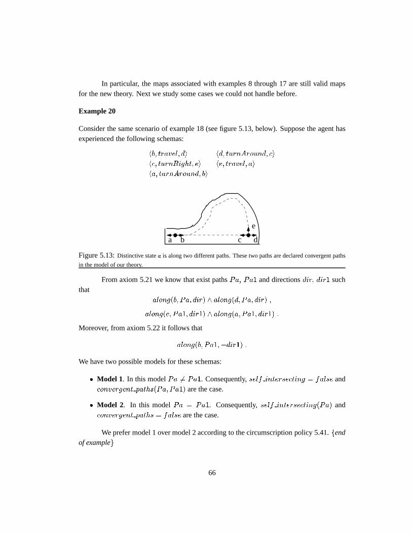
In particular, the maps associated with examples 8 through 17 are still valid mapsfor the new theory. Next we study some cases we could not handle before.

Example 20

Consider the same scenario of example 18 (see figure 5.13, below). Suppose the agent hasexperienced the following schemas:

hb; travel; di hd; turnAround; ci

hc; turnRight; ei he; travel; ai

ha; turnAround; bi

a b d

e

c

Figure 5.13:Distinctive statea is along two different paths. These two paths are declared convergent paths

in the model of our theory.

From axiom 5.21 we know that exist pathsPa; Pa1 and directionsdir; dir1 suchthat

along(b; Pa; dir) ^ along(d; Pa; dir) ;

along(e; Pa1; dir1) ^ along(a; Pa1; dir1) :

Moreover, from axiom 5.22 it follows that

along(b; Pa1;�dir1) :

We have two possible models for these schemas:

� Model 1. In this modelPa 6= Pa1. Consequently,self intersecting = false andconvergent paths(Pa; Pa1) are the case.

� Model 2. In this modelPa = Pa1. Consequently,self intersecting(Pa) andconvergent paths = false are the case.

We prefer model 1 over model 2 according to the circumscription policy 5.41.fendof exampleg

66

(a) (b)

c

a b d

Figure 5.14:The environment in (a) can be described by two different topological maps. Either as a long

straight path and a curved path, or as a short straight path and a long curved path.

Example 21

Whenever convergent paths exist, the theory will have multiple models. Consider the set

of schemas (see figure 5.14)h a; travel; b i h b; travel; d i,h a; turnLeft; c i h c; travel; b i, h b; travel; d i.

These

schemas will have the following two models, which differ in the paths they use to explainthe travel axioms:

1. a-b-d, c-b

2. c-b-d, a-b

Notice that in both cases the shorter path will not include the tuple b-d. This comes fromthe minimization ofalong. The minimization oftpath also plays a role, since otherwiseone could have a three paths modelfa-b, c-b, b-dg.

Suppose one has the extra schemahd; travel; ei. In this case the models will beextensions of the both above:

1. a-b-d-e, c-b

2. c-b-d-e, a-b

fend of exampleg

In order to compare any two possible maps, these maps must have a common sortof places and paths. Since a map can be arbitrarily large, no finite domain can be adequateand so we require the sorts of places and paths to be infinite. This requirement makes thethe circumscription policy 5.41 to behave as expected. Consider the following example (seealso theorem 5, page 46).

Example 22

67

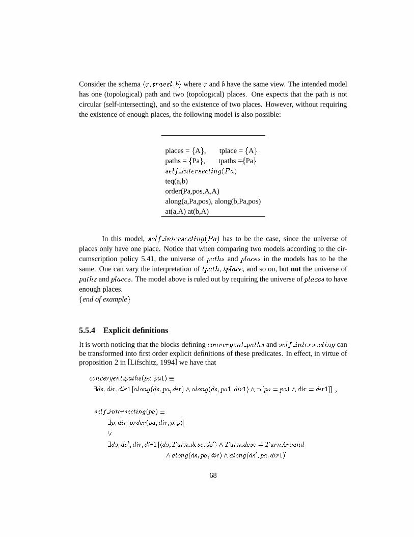
Consider the schemaha; travel; bi wherea andb have the same view. The intended modelhas one (topological) path and two (topological) places. One expects that the path is notcircular (self-intersecting), and so the existence of two places. However, without requiringthe existence of enough places, the following model is also possible:

places =fAg, tplace =fAgpaths =fPag, tpaths =fPagself intersecting(Pa)

teq(a,b)order(Pa,pos,A,A)along(a,Pa,pos), along(b,Pa,pos)at(a,A) at(b,A)

In this model,self intersecting(Pa) has to be the case, since the universe ofplaces only have one place. Notice that when comparing two models according to the cir-cumscription policy 5.41, the universe ofpaths andplaces in the models has to be thesame. One can vary the interpretation oftpath, tplace, and so on, butnot the universe ofpaths andplaces. The model above is ruled out by requiring the universe ofplaces to haveenough places.fend of exampleg

5.5.4 Explicit definitions

It is worth noticing that the blocks definingconvergent paths andself intersecting canbe transformed into first order explicit definitions of these predicates. In effect, in virtue ofproposition 2 in[Lifschitz, 1994] we have that

convergent paths(pa; pa1) �

9ds; dir; dir1 [along(ds; pa; dir) ^ along(ds; pa1; dir1) ^ : [pa = pa1 ^ dir = dir1]] ;

self intersecting(pa) �

9p; dir [order(pa; dir; p; p)]

_

9ds; ds0; dir; dir1 [hds; Turn desc; ds0i ^ Turn desc 6= TurnAround

^ along(ds; pa; dir) ^ along(ds0; pa; dir1)]

68

_

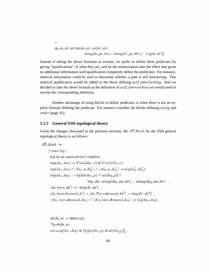
9p; ds; ds0; dir [at(ds; p) ^ at(ds0; p)^

along(ds; pa; dir) ^ along(ds0; pa; dir) ^ :teq(ds; ds0)]

Instead of taking the above formulas as axioms, we prefer to define these predicates bygiving “qualifications” of what they are, and let the minimization take the effect that givenno additional information such qualification completely define the predicates. For instance,metrical information could be used to determine whether a path is self intersecting. Thismetrical qualification would be added to the block definingself intersecting. Had wedecided to take the above formula as the definition ofself intersecting we would need torewrite the corresponding definition.

Another advantage of using blocks to define predicates is when there is not an ex-plicit formula defining the predicate. For instance consider the blocks definingalong andorder (page 41).

5.5.5 General SSH topological theory

Given the changes discussed in the previous sections, theAT block for the SSH generaltopological theory is as follows:

AT block =

f max teq :

teq is an equivalence relation ;

teq(ds1; ds2)! V iew(ds1; v) � V iew(ds2; v);

teq(ds1; ds2) ^ h ds1; a; ds01 i ^ h ds2; a; ds

02 i ! teq(ds01; ds

02);

teq(ds1; ds2)! 8p [at(ds1; p) � at(ds2; p)] ^

8pa; dir [along(ds1; pa; dir) � along(ds2; pa; dir)] ;

hds; turn; ds0i ! :teq(ds; ds0) ;

hds; turnAround; ds0i ^ hds; TurnAround; ds00i ! teq(ds0; ds00) ;

h ds1; turnAround; ds2 i ^ h ds2; turnAround; ds3 i ! teq(ds1; ds3) ;

at(ds; p)! tplace(p);

9!p at(ds; p);

turn eq(ds1; ds2) � 8p [at(ds1; p) � at(ds2; p)] ;

69

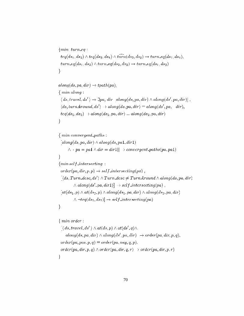
fmin turn eq :

teq(ds1; ds2) ^ teq(ds3; ds4) ^ dturn(ds2; ds3)! turn eq(ds1; ds4);

turn eq(ds1; ds2) ^ turn eq(ds2; ds3)! turn eq(ds1; ds3)

g

along(ds; pa; dir)! tpath(pa);

f min along :

h ds; travel; ds0 i ! 9pa; dir�along(ds; pa; dir) ^ along(ds0; pa; dir)

�;

hds; turnAround; ds0i ! along(ds; pa; dir) � along(ds0; pa;�dir);

teq(ds1; ds2)! along(ds1; pa; dir) � along(ds2; pa; dir)

g

f min convergent paths :

[along(ds; pa; dir) ^ along(ds; pa1; dir1)

^: [pa = pa1 ^ dir = dir1]]! convergent paths(pa; pa1)

g

fmin self intersecting :

order(pa; dir; p; p)! self intersecting(pa) ;�hds; Turn desc; ds0i ^ Turn desc 6= TurnAround ^ along(ds; pa; dir)

^ along(ds0; pa; dir1)�! self intersecting(pa) ;

[at(ds1; p) ^ at(ds2; p) ^ along(ds1; pa; dir) ^ along(ds2; pa; dir)

^ :teq(ds1; ds2)]! self intersecting(pa)

g

f min order :�h ds; travel; ds0 i ^ at(ds; p) ^ at(ds0; q)^

along(ds; pa; dir) ^ along(ds0; pa; dir)�! order(pa; dir; p; q);

order(pa; pos; p; q) � order(pa; neg; q; p);

order(pa; dir; p; q) ^ order(pa; dir; q; r)! order(pa; dir; p; r)

g

70

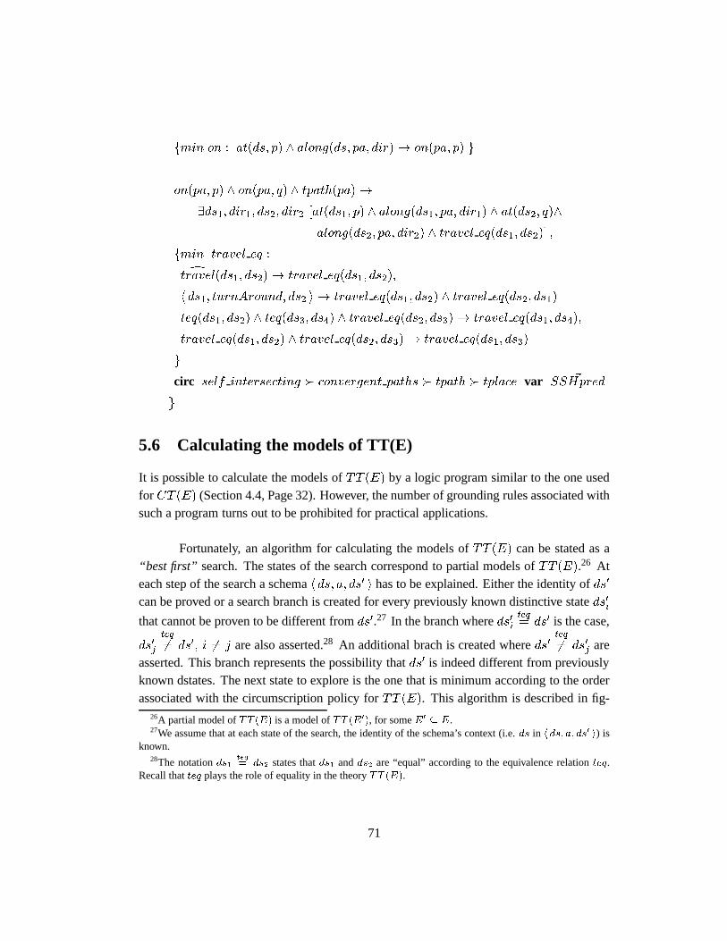
fmin on : at(ds; p) ^ along(ds; pa; dir)! on(pa; p) g

on(pa; p) ^ on(pa; q) ^ tpath(pa)!

9ds1; dir1; ds2; dir2 [at(ds1; p) ^ along(ds1; pa; dir1) ^ at(ds2; q)^

along(ds2; pa; dir2) ^ travel eq(ds1; ds2)] ;

fmin travel eq :dtravel(ds1; ds2)! travel eq(ds1; ds2);

h ds1; turnAround; ds2 i ! travel eq(ds1; ds2) ^ travel eq(ds2; ds1)

teq(ds1; ds2) ^ teq(ds3; ds4) ^ travel eq(ds2; ds3)! travel eq(ds1; ds4);

travel eq(ds1; ds2) ^ travel eq(ds2; ds3)! travel eq(ds1; ds3)

g

circ self intersecting � convergent paths � tpath � tplace var ~SSHpred

g

5.6 Calculating the models of TT(E)

It is possible to calculate the models ofTT (E) by a logic program similar to the one usedfor CT (E) (Section 4.4, Page 32). However, the number of grounding rules associated withsuch a program turns out to be prohibited for practical applications.

Fortunately, an algorithm for calculating the models ofTT (E) can be stated as a“best first” search. The states of the search correspond to partial models ofTT (E).26 Ateach step of the search a schemah ds; a; ds0 i has to be explained. Either the identity ofds0

can be proved or a search branch is created for every previously known distinctive stateds0ithat cannot be proven to be different fromds0.27 In the branch whereds0i

teq= ds0 is the case,

ds0jteq

6= ds0; i 6= j are also asserted.28 An additional brach is created whereds0teq

6= ds0j areasserted. This branch represents the possibility thatds0 is indeed different from previouslyknown dstates. The next state to explore is the one that is minimum according to the orderassociated with the circumscription policy forTT (E). This algorithm is described in fig-

26A partial model ofTT (E) is a model ofTT (E0), for someE0 � E.27We assume that at each state of the search, the identity of the schema’s context (i.e.ds in hds; a; ds0 i) is

known.28The notationds1

teq= ds2 states thatds1 andds2 are “equal” according to the equivalence relationteq.

Recall thatteq plays the role of equality in the theoryTT (E).

71

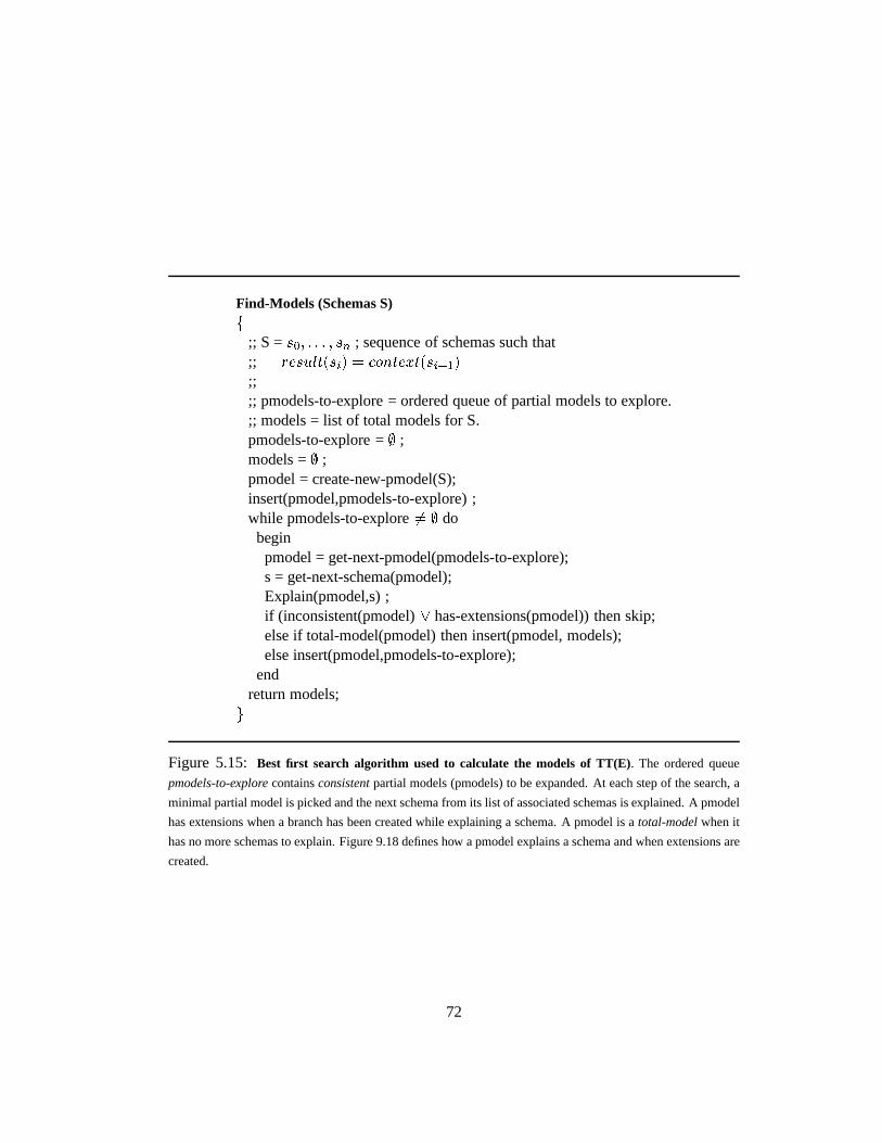
Find-Models (Schemas S)f

;; S =s0; : : : ; sn ; sequence of schemas such that;; result(si) = context(si+1);;;; pmodels-to-explore = ordered queue of partial models to explore.;; models = list of total models for S.pmodels-to-explore =; ;models =; ;pmodel = create-new-pmodel(S);insert(pmodel,pmodels-to-explore) ;while pmodels-to-explore6= ; dobeginpmodel = get-next-pmodel(pmodels-to-explore);s = get-next-schema(pmodel);Explain(pmodel,s) ;if (inconsistent(pmodel)_ has-extensions(pmodel)) then skip;else if total-model(pmodel) then insert(pmodel, models);else insert(pmodel,pmodels-to-explore);

endreturn models;g

Figure 5.15: Best first search algorithm used to calculate the models of TT(E). The ordered queue

pmodels-to-explorecontainsconsistentpartial models (pmodels) to be expanded. At each step of the search, a

minimal partial model is picked and the next schema from its list of associated schemas is explained. A pmodel

has extensions when a branch has been created while explaining a schema. A pmodel is atotal-modelwhen it

has no more schemas to explain. Figure 9.18 defines how a pmodel explains a schema and when extensions are

created.

72

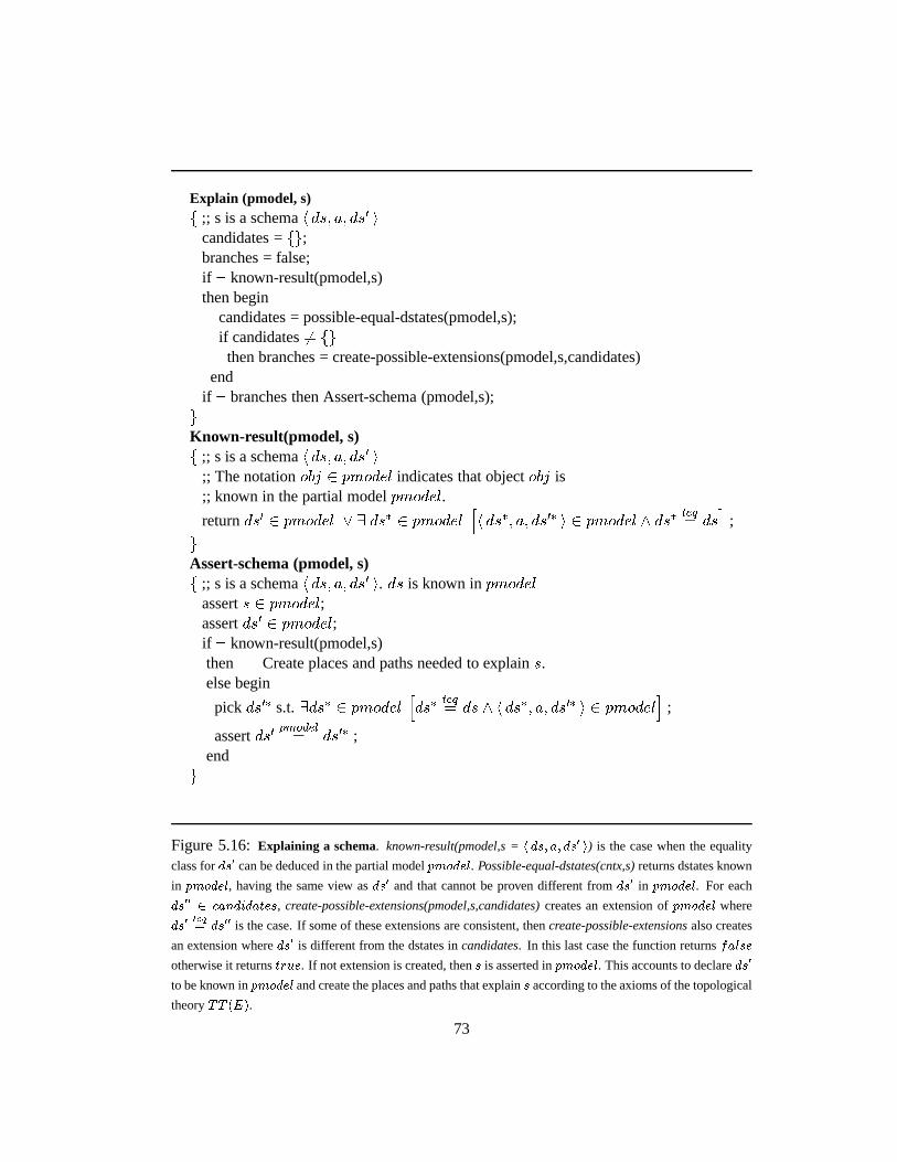
Explain (pmodel, s)f ;; s is a schemah ds; a; ds0 i

candidates =fg;branches = false;if : known-result(pmodel,s)then begin

candidates = possible-equal-dstates(pmodel,s);if candidates6= fgthen branches = create-possible-extensions(pmodel,s,candidates)

endif : branches then Assert-schema (pmodel,s);gKnown-result(pmodel, s)f ;; s is a schemah ds; a; ds0 i

;; The notationobj 2 pmodel indicates that objectobj is;; known in the partial modelpmodel.

returnds0 2 pmodel _ 9 ds� 2 pmodelhh ds�; a; ds0� i 2 pmodel ^ ds�

teq= ds

i;

gAssert-schema (pmodel, s)f ;; s is a schemah ds; a; ds0 i. ds is known inpmodel

asserts 2 pmodel;assertds0 2 pmodel;if : known-result(pmodel,s)then Create places and paths needed to explains.else begin

pick ds0� s.t.9ds� 2 pmodelhds�

teq= ds ^ h ds�; a; ds0� i 2 pmodel

i;

assertds0pmodel= ds0� ;

endg

Figure 5.16:Explaining a schema. known-result(pmodel,s =h ds; a; ds0 i) is the case when the equality

class fords0 can be deduced in the partial modelpmodel. Possible-equal-dstates(cntx,s)returns dstates known

in pmodel, having the same view asds0 and that cannot be proven different fromds0 in pmodel. For each

ds00 2 candidates, create-possible-extensions(pmodel,s,candidates)creates an extension ofpmodel where

ds0teq= ds00 is the case. If some of these extensions are consistent, thencreate-possible-extensionsalso creates

an extension whereds0 is different from the dstates incandidates. In this last case the function returnsfalse

otherwise it returnstrue. If not extension is created, thens is asserted inpmodel. This accounts to declareds0

to be known inpmodel and create the places and paths that explains according to the axioms of the topological

theoryTT (E).

73

ures 5.15 and 5.16.29 See section 9.4.2, page 152, for a discussion on the implementationof this algorithm.

29A search state is implemented by a partial model,pmodel. Branches in the search are represented bycreatingextensionsfor the current search state (pmodel). Thatpmodel0 is an extension ofpmodel implies thatpmodel0 inherits frompmodel all known objects and facts. Partial models are described in page 155.

74

5.7 Summary

Actions performed by the agent are categorized at the SSH topological level into twoclasses: turn and travel. Turn actions leave the agent at the same place. Travel actionsmove the agent to a new place along a path. The SSH topological map is derived fromthe agent’s experiences by creating the minimum set of paths and places explaining suchexperiences. In this chapter we have made precise this minimality criterion by specifying(via circumscription) the preferred models associated with the SSH topological level.

The concepts ofpath andplacecan be used to distinguish environment states thatare not distinguishable by actions and views alone. In addition, we have illustrated howthe agent’s topological map changes as the agent acquires more experiences in the environ-ment. These changes are non-monotonic as the agent can conclude, for example, that twopreviously believed different places are indeed the same (or vice versa).

It is possible that more than one topological map is consistent with the agent’s setof experiences. In order to disambiguate the topological map, the agent must collect newexperiences or rely on other sources of information to disambiguate its map (for example,metrical information or regions). It is also possible that there is no topological map consis-tent with the agent’s experiences: this happens for example if the agent travels in a loop,violating our assumption that paths are not self-intersecting. This is not to say that we as-sume “rectilinear” environments where paths intersect at most in one place. As example 17(page 55) shows, paths can intersect in more that one place. Another reason for not havinga topological map are patterns of experience in which known different paths merge into thesame distinctive state (i.e. convergent paths).

In section 5.5 we defined a general topological theory where self-intersecting andconvergent paths were included. The general theory extended the more restricted one in thesense that a map according to the later is a map according to the former. The new theorycaptures the intuition that by default paths are not self-intersercting or convergent.

Finally, in section 5.6 we stated the problem of finding the models ofTT (E) asa “best first” search. In this search, the next state to explore is the one that is minimumaccording to the order associated with the circumscription policy forTT (E). We definedthe main elements of this search and postponed further details to the implementation chapter(section 9.4.2, page 152). The algorithm here described allows the agent to keep trackof different possible models (maps) as well as to recover from distinctive state equality

75

assumptions that make a model inconsistent.

76

Chapter 6

Boundary Regions

Topological paths play the role ofstreetsin a city layout map. Streets are often used as areference for specifying the location of a given place: a place will be either on the givenstreet or in one of the “two sides” –left or right– of the street.

Mathematically, the concept of left and right of a SSH topological path is relatedto the topological one of the interior and exterior of a curve. While not all curves have awell defined interior and exterior (for example, consider a spiral, or a fractal curve), closednot self-intersecting1 curves –Jordan curves– do have associated interior and exterior sets[Beardon, 1979].2 Moreover, in order to go from the interior to the exterior (or vice versa)of the curve , one has to cross .3 Our analogy of SSH topological paths and mathemati-cal curves breaks down because in general the agent might be able to travel from one sideof the path to the other without crossing the path. This can happen because of the agent’sinability to detect that it has crossed the path, or (more often) because paths are not longenough to divide the environment into two regions (for example, consider a dead-end street).

In order to determine boundary relations -the location of a place with respect to apath- we formally state the following heuristic. Suppose the agent is at an intersection on agiven path, and it then turns right. If the agent now travels, any place it finds while travelingwith no turns will be on the right of the starting path. While this heuristic draws the correctconclusion in a rectilinear environment, it may draw incorrect conclusions when paths arenot straight. Consequently, we state our heuristic as a ‘defeasible” rule (default) so as not

1Except of course for the end points of the curve.2When the curve is removed, the plane is divided into two disjoint connected sets.3Given a curve 0 - a continuous function 0 : [0; 1]! R2 - such that there existt1 andt2, 0(t1) 2 interior

of , 0(t2) 2 exterior of , then there existt andt0 such that (t) = 0(t0).

77

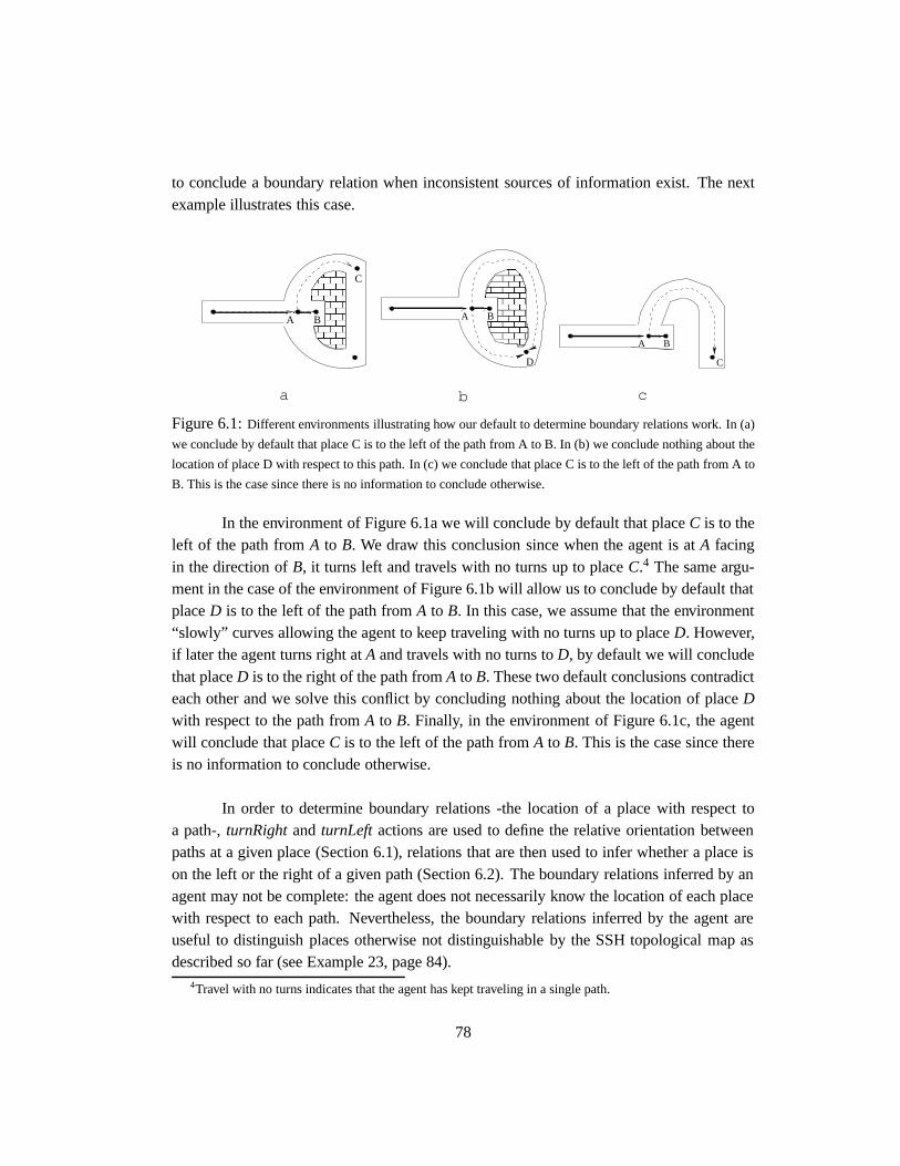
to conclude a boundary relation when inconsistent sources of information exist. The nextexample illustrates this case.

���������������������

���������������������

B

C

A

����������������������������

����������������������������

BA

D

BA

C

a b c

Figure 6.1:Different environments illustrating how our default to determine boundary relations work. In (a)

we conclude by default that place C is to the left of the path from A to B. In (b) we conclude nothing about the

location of place D with respect to this path. In (c) we conclude that place C is to the left of the path from A to

B. This is the case since there is no information to conclude otherwise.

In the environment of Figure 6.1a we will conclude by default that placeC is to theleft of the path fromA to B. We draw this conclusion since when the agent is atA facingin the direction ofB, it turns left and travels with no turns up to placeC.4 The same argu-ment in the case of the environment of Figure 6.1b will allow us to conclude by default thatplaceD is to the left of the path fromA to B. In this case, we assume that the environment“slowly” curves allowing the agent to keep traveling with no turns up to placeD. However,if later the agent turns right atA and travels with no turns toD, by default we will concludethat placeD is to the right of the path fromA to B. These two default conclusions contradicteach other and we solve this conflict by concluding nothing about the location of placeDwith respect to the path fromA to B. Finally, in the environment of Figure 6.1c, the agentwill conclude that placeC is to the left of the path fromA to B. This is the case since thereis no information to conclude otherwise.

In order to determine boundary relations -the location of a place with respect toa path-,turnRightand turnLeft actions are used to define the relative orientation betweenpaths at a given place (Section 6.1), relations that are then used to infer whether a place ison the left or the right of a given path (Section 6.2). The boundary relations inferred by anagent may not be complete: the agent does not necessarily know the location of each placewith respect to each path. Nevertheless, the boundary relations inferred by the agent areuseful to distinguish places otherwise not distinguishable by the SSH topological map asdescribed so far (see Example 23, page 84).

4Travel with no turns indicates that the agent has kept traveling in a single path.

78

6.1 Qualitative orientation of paths at a place

We extend the topological level in order to represent the relative orientation among pathsthat intersect at a given place. We use the predicates

totheLeftOf(p; pa; dir; pa1; dir1) ; totheRightOf(p; pa; dir; pa1; dir1)

to represent the facts that (i)p is aplaceon both paths,paandpa1, and (ii), when the agentis atplace pfacing on the directiondir of pa, after executing a turn left (right) action, theagent will be facing on the directiondir1 of pa1(see Figure 6.2, Page 80).

The predicatestotheLeftOf andtotheRightOf are derived from the actions per-formed by the agent at a place:5

fmin totheRightOf; min totheLeftOf : (6.1)

[hds; turnRight; ds1i ^ at(ds; p) ^ along(ds; pa; dir) ^ along(ds1; pa1; dir1)]

! totheRightOf(p; pa; dir; pa1; dir1);

[hds; turnLeft; ds1i ^ at(ds; p) ^ along(ds; pa; dir) ^ along(ds1; pa1; dir1)]

! totheLeftOf(p; pa; dir; pa1; dir1):

g

6.2 Left and Right of a path

A path has associated two regions: the places to the left of the path and the places to theright of the path.6 We use the predicates

leftOf(pa; dir; lr) ; rightOf(pa; dir; rr)

to denote thatregion lr (rr) is the left (right) region of pathpa with respect to the path’sdirectiondir. The properties of these predicate are as follows:

9!lr fleftOf(pa; dir; lr)g ; 9!rr frightOf(pa; dir; rr)g (6.2)

leftOf(pa; dir; r) � rightOf(pa;�dir; r) (6.3)

fmin is region : (6.4)

LeftOf(pa; dir; lr)! is region(lr)

g

leftOf(pa; dir; lr) ^ leftOf(pa1; dir1; lr)! pa = pa1 (6.5)5It is possible that the agent learns these relations by being told. In the presence of no other information,

the implications in block 6.1 become equivalences (proposition 2 in[Lifschitz, 1994]).6Regions are set of places or regions. This way, regions form a containment hierarchy that allows the

agent to reason at different levels of detail about its spatial representation. In Chapter 8 we present a completeformalization of regions in the context of the SSH.

79

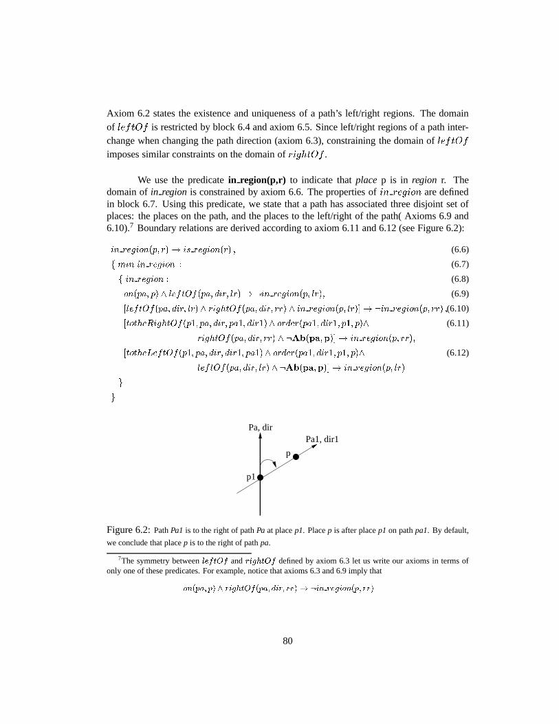
Axiom 6.2 states the existence and uniqueness of a path’s left/right regions. The domainof leftOf is restricted by block 6.4 and axiom 6.5. Since left/right regions of a path inter-change when changing the path direction (axiom 6.3), constraining the domain ofleftOf

imposes similar constraints on the domain ofrightOf .

We use the predicatein region(p,r) to indicate thatplace p is in region r. Thedomain ofin region is constrained by axiom 6.6. The properties ofin region are definedin block 6.7. Using this predicate, we state that a path has associated three disjoint set ofplaces: the places on the path, and the places to the left/right of the path( Axioms 6.9 and6.10).7 Boundary relations are derived according to axiom 6.11 and 6.12 (see Figure 6.2):

in region(p; r)! is region(r) ; (6.6)

f min in region : (6.7)

f in region : (6.8)

on(pa; p) ^ leftOf(pa; dir; lr)! :in region(p; lr); (6.9)

[leftOf(pa; dir; lr) ^ rightOf(pa; dir; rr) ^ in region(p; lr)]! :in region(p; rr) ;(6.10)

[totheRightOf(p1; pa; dir; pa1; dir1)^ order(pa1; dir1; p1; p)^ (6.11)

rightOf(pa; dir; rr) ^ :Ab(pa;p)]! in region(p; rr);

[totheLeftOf(p1; pa; dir; dir1; pa1)^ order(pa1; dir1; p1; p)^ (6.12)

leftOf(pa; dir; lr) ^ :Ab(pa;p)]! in region(p; lr)

g

g

p

p1

Pa, dirPa1, dir1

Figure 6.2:PathPa1 is to the right of pathPa at placep1. Placep is after placep1 on pathpa1. By default,

we conclude that placep is to the right of pathpa.

7The symmetry betweenleftOf andrightOf defined by axiom 6.3 let us write our axioms in terms ofonly one of these predicates. For example, notice that axioms 6.3 and 6.9 imply that

on(pa; p) ^ rightOf(pa; dir; rr)! :in region(p; rr)

80

The outer block 6.7 states that normally boundary relations are false. This is thecase since by default the agent does not know the location of a place with respect to a givenpath. The inner block 6.8 states under what conditions the agent can derive a boundaryrelation. For instance, according to axiom 6.11, if at placep1 pathpa1 is to the right ofpathpa, and placep is afterp1 on pathpa1, then normally it is the case thatp is on theright of pa (see Figure 6.2).8 The predicateAb inside block 6.8 is the standard “abnor-mality” predicate used to represent defaults in circumscriptive theories ([McCarthy, 1980,Lifschitz, 1994], see Appendix C, Page 219).

While block 6.7 defines the extent of the predicatein region, it does not expressour preference for models wherein region is maximal. We need to includein region inour circumscription policy, as shown in the next section. In order to understand why this isthe case, assumeAb = false inside block 6.8. Consequently, block 6.7 becomes

f min in region :

on(pa; p) ^ leftOf(pa; dir; lr)! :in region(p; lr) ;

[leftOf(pa; dir; lr) ^ rightOf(pa; dir; rr) ^ in region(p; lr)]! :in region(p; rr) ;

[totheRightOf(p1; pa; dir; pa1; dir1)^ order(pa1; dir1; p1; p)^

rightOf(pa; dir; rr)]! in region(p; rr) ;

[toTheLeftof(p1; pa; dir; dir1; pa1)^ order(pa1; dir1; p1; p)^

leftOf(pa; dir; lr)]! in region(p; lr)

g

This block can be further simplified as follows (see Propositions 2 and 4 in[Lifschitz, 1994]):

on(pa; p) ^ leftOf(pa; dir; lr)! :in region(p; lr) ;

[leftOf(pa; dir; lr) ^ rightOf(pa; dir; rr) ^ in region(p; lr)]! :in region(p; rr) ;

in region(p; r)

�

9p1; pa; dir; pa1; dir1f

[totheRightOf(p1; pa; dir; pa1; dir1)^ order(pa1; dir1; p1; p) ^ rightOf(pa; dir; r)]

_

[toTheLeftof(p1; pa; dir; dir1; pa1)^ order(pa1; dir1; p1; p) ^ leftOf(pa; dir; r)]

g :

Since block 6.7 “normally” is equivalent to the statements above, and so, it “normally”8See appendix C, page 219, for a similar formalization of the standard example: objects normally do not

fly; birds normally do.

81

reduces to an explicit definition forin region, block 6.7 does not express our preferencefor models wherein region is maximal, preference that has to be expressed elsewhere (seenext section).9

6.2.1 Adding boundary relations to the topological map

In order to use boundary relations when defining the SSH topological map, axioms 6.1-6.12are included inside the blockAT block (see Section 5.1, page 41), and the new circumscrip-tion policy becomes10

circ tpath � :in region � tplace var ~newSSHpred

where ~newSSHpred stands for the tuple of predicates

h at; along; order; on; teq; turn eq; travel eq;

totheRightOf ; totheLeftOf ; leftOf ; rightOf ; is region

i :

The circumscription policy states that axioms 6.11 and 6.12 should be used to draw conclu-sions even at the expense of having more places on the map. This is achieved by maximizingin region overtplace in the circumscription policy. Next we show the new theory.

AT block =

f max teq :

Axioms 6.1-6.12;

teq is an equivalence relation ;

teq(ds1; ds2)! V iew(ds1; v) � V iew(ds2; v);

teq(ds1; ds2) ^ h ds1; a; ds0

1 i ^ h ds2; a; ds0

2 i ! teq(ds01; ds0

2);

teq(ds1; ds2)! 8p [at(ds1; p) � at(ds2; p)] ^

8pa; dir [along(ds1; pa; dir) � along(ds2; pa; dir)] ;

hds; turn; ds0i ! :teq(ds; ds0) ;

hds; turnAround; ds0i ^ hds; TurnAround; ds00i ! teq(ds0; ds00) ;

h ds1; turnAround; ds2 i ^ h ds2; turnAround; ds3 i ! teq(ds1; ds3) ;

at(ds; p)! tplace(p);

9!p at(ds; p);

9Notice that the statements above are the ones characterizing boundary relations in “rectilinear”environments.

10See circumscription notation in page 222.

82

turn eq(ds1; ds2) � 8p [at(ds1; p) � at(ds2; p)] ;

fmin turn eq :

teq(ds1; ds2) ^ teq(ds3; ds4) ^ dturn(ds2; ds3)! turn eq(ds1; ds4);

turn eq(ds1; ds2) ^ turn eq(ds2; ds3)! turn eq(ds1; ds3)

g

along(ds; pa; dir)! tpath(pa);

f min along :

h ds; travel; ds0 i ! 9pa; dir [along(ds; pa; dir) ^ along(ds0; pa; dir)] ;

hds; turnAround; ds0i ! along(ds; pa; dir) � along(ds0; pa;�dir);

teq(ds1; ds2)! along(ds1; pa; dir) � along(ds2; pa; dir)

g

along(ds; pa; dir) ^ along(ds; pa1; dir1)! pa = pa1 ^ dir = dir1;

at(ds1; p) ^ at(ds2; p) ^ along(ds1; pa; dir) ^ along(ds2; pa; dir)! teq(ds1; ds2);

[hds; turn desc; ds0i ^ turn desc 6= turnAround ^

along(ds; pa; dir) ^ along(ds0; pa1; dir1)]! pa 6= pa1;

f min order :

[h ds; travel; ds0 i ^ at(ds; p) ^ at(ds0; q)^

along(ds; pa; dir) ^ along(ds0; pa; dir)]! order(pa; dir; p; q);

order(pa; pos; p; q) � order(pa; neg; q; p);

order(pa; dir; p; q) ^ order(pa; dir; q; r) ! order(pa; dir; p; r)

g

:order(pa; dir; p; p);

fmin on : at(ds; p) ^ along(ds; pa; dir)! on(pa; p) g

on(pa; p) ^ on(pa; q) ^ tpath(pa)!

9ds1; dir1; ds2; dir2 [at(ds1; p) ^ along(ds1; pa; dir1) ^ at(ds2; q)^

along(ds2; pa; dir2) ^ travel eq(ds1; ds2)] ;

fmin travel eq :dtravel(ds1; ds2)! travel eq(ds1; ds2);

h ds1; turnAround; ds2 i ! travel eq(ds1; ds2) ^ travel eq(ds2; ds1);

teq(ds1; ds2) ^ teq(ds3; ds4) ^ travel eq(ds2; ds3)! travel eq(ds1; ds4);

83

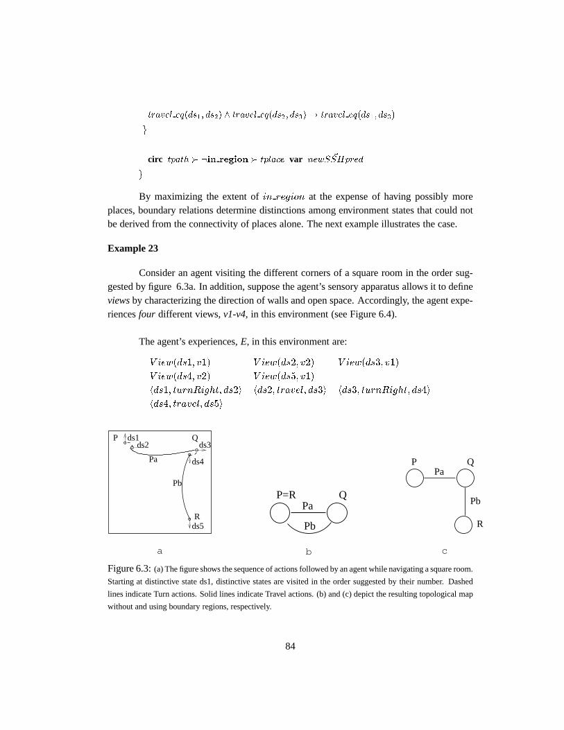
travel eq(ds1; ds2) ^ travel eq(ds2; ds3)! travel eq(ds1; ds3)

g

circ tpath � :in region � tplace var ~newSSHpred

g

By maximizing the extent ofin region at the expense of having possibly moreplaces, boundary relations determine distinctions among environment states that could notbe derived from the connectivity of places alone. The next example illustrates the case.

Example 23

Consider an agent visiting the different corners of a square room in the order sug-gested by figure 6.3a. In addition, suppose the agent’s sensory apparatus allows it to defineviewsby characterizing the direction of walls and open space. Accordingly, the agent expe-riencesfour different views,v1-v4, in this environment (see Figure 6.4).

The agent’s experiences,E, in this environment are:

V iew(ds1; v1) V iew(ds2; v2) V iew(ds3; v1)

V iew(ds4; v2) V iew(ds5; v1)

hds1; turnRight; ds2i hds2; travel; ds3i hds3; turnRight; ds4i

hds4; travel; ds5i

P ds1ds2

Pa

ds3

Pb

Rds5

ds4

Q

Pb

PaQP=R

R

Pb

PaQP

a b c

Figure 6.3:(a) The figure shows the sequence of actions followed by an agent while navigating a square room.

Starting at distinctive state ds1, distinctive states are visited in the order suggested by their number. Dashed

lines indicate Turn actions. Solid lines indicate Travel actions. (b) and (c) depict the resulting topological map

without and using boundary regions, respectively.

84

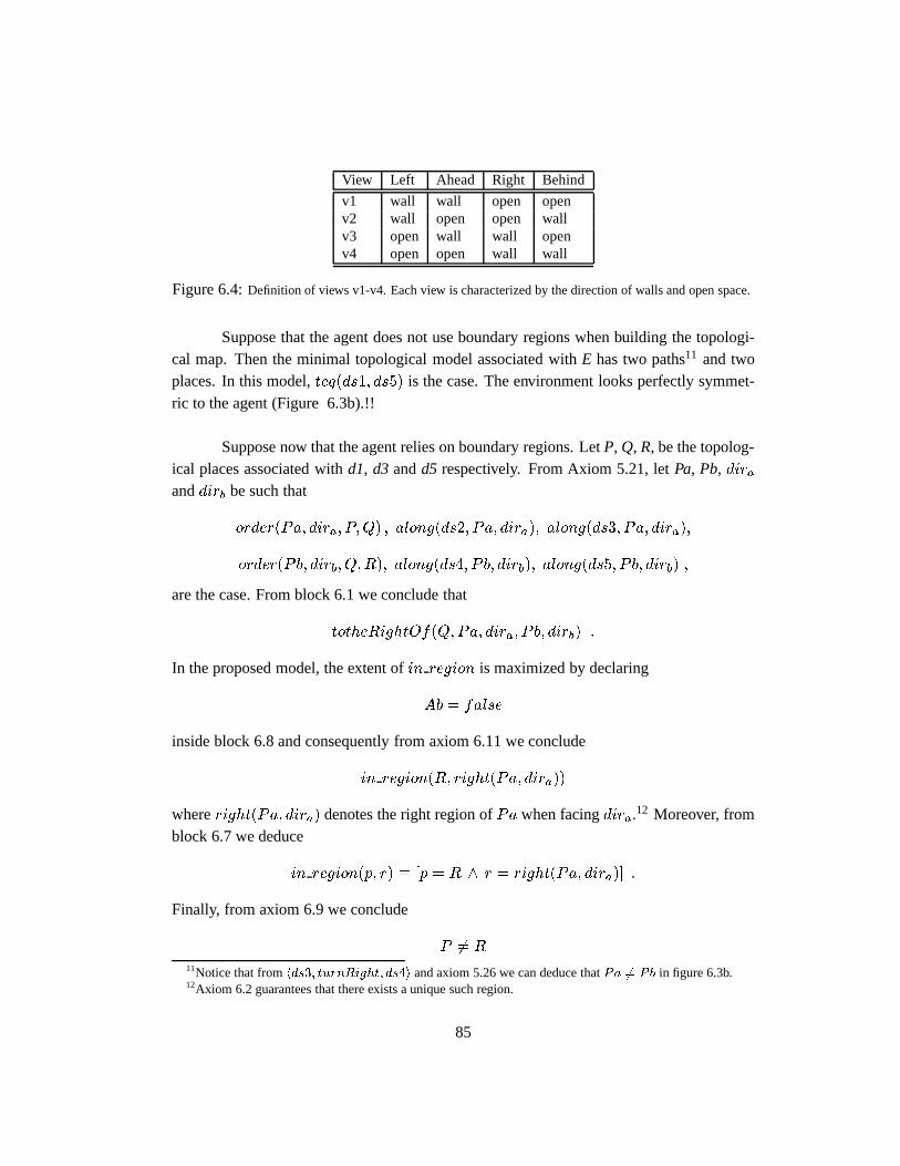
View Left Ahead Right Behind

v1 wall wall open openv2 wall open open wallv3 open wall wall openv4 open open wall wall

Figure 6.4:Definition of views v1-v4. Each view is characterized by the direction of walls and open space.

Suppose that the agent does not use boundary regions when building the topologi-cal map. Then the minimal topological model associated withE has two paths11 and twoplaces. In this model,teq(ds1; ds5) is the case. The environment looks perfectly symmet-ric to the agent (Figure 6.3b).!!

Suppose now that the agent relies on boundary regions. LetP, Q, R, be the topolog-ical places associated withd1, d3 andd5 respectively. From Axiom 5.21, letPa, Pb, diraanddirb be such that

order(Pa; dira; P;Q) ; along(ds2; Pa; dira); along(ds3; Pa; dira);

order(Pb; dirb; Q;R); along(ds4; P b; dirb); along(ds5; P b; dirb) ;

are the case. From block 6.1 we conclude that

totheRightOf(Q;Pa; dira; P b; dirb) :

In the proposed model, the extent ofin region is maximized by declaring

Ab = false

inside block 6.8 and consequently from axiom 6.11 we conclude

in region(R; right(Pa; dira))

whereright(Pa; dira) denotes the right region ofPa when facingdira.12 Moreover, fromblock 6.7 we deduce

in region(p; r) � [p = R ^ r = right(Pa; dira)] :

Finally, from axiom 6.9 we conclude

P 6= R

11Notice that fromhds3; turnRight; ds4i and axiom 5.26 we can deduce thatPa 6= Pb in figure 6.3b.12Axiom 6.2 guarantees that there exists a unique such region.

85

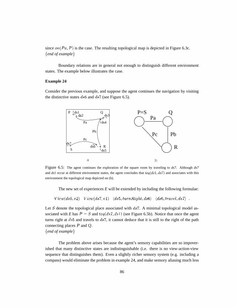
sinceon(Pa; P ) is the case. The resulting topological map is depicted in Figure 6.3c.fend of exampleg

Boundary relations are in general not enough to distinguish different environmentstates. The example below illustrates the case.

Example 24

Consider the previous example, and suppose the agent continues the navigation by visitingthe distinctive statesds6 andds7 (see Figure 6.5).

ds7

S

ds2ds1P

ds3

ds6ds5

R

Pc

Pa

Pb

ds4

Q

R

Pb

QPa

P=S

Pc

a b

Figure 6.5: The agent continues the exploration of the square room by traveling tods7. Although ds7

andds1occur at different environment states, the agent concludes thatteq(ds1; ds7) and associates with this

environment the topological map depicted on (b).

The new set of experiencesE will be extended by including the following formulae:

V iew(ds6; v2) V iew(ds7; v1) hds5; turnRight; ds6i hds6; travel; ds7i :

Let S denote the topological place associated withds7. A minimal topological model as-sociated withE hasP = S andteq(ds7; ds1) (see Figure 6.5b). Notice that once the agentturns right atds5 and travels tods7, it cannot deduce that it is still to the right of the pathconnecting placesP andQ.fend of exampleg

The problem above arises because the agent’s sensory capabilities are so impover-ished that many distinctive states are indistinguishable (i.e. there is no view-action-viewsequence that distinguishes them). Even a slightly richer sensory system (e.g. including acompass) would eliminate the problem in example 24, and make sensory aliasing much less

86

common globally. The problem cannot be eliminated entirely through better sensors, sincesome environment states may be genuinely indistinguishable by any given set of sensors.

How can the agent realize thatds7 and ds1 in the previous example are indeeddifferent environment states?. This apparently easy problem turns out to be a hard one.Next we summarize different approaches to solve this problem:

� The agent can gather more information as in theRehearsal procedureproposed in[Kuipers and Byun, 1988]. In order to disambiguate two distinctive states the agentfinds a sequence of actions and views that prove (or disprove) that the agent is at agiven distinctive state. Once that sequence is found, the agent performs the actions inthe sequence and checks whether it obtains the expected views. If some of the viewsobtained during the navigation do not match the expected views, the agent concludesthat it was not at the hypothesized distinctive state. If all of the views match the ex-pected views, the agent cannot conclude anything about its starting distinctive state.This method has three drawbacks: (i) the disambiguating sequence may not exist (asin Example 24), (ii) the method is partially conclusive, and (iii), it requires physicalnavigation. While a partially conclusive method, richer sensors will increase the ef-fectiveness of the rehearsal procedure.

The rehearsal procedure is closely related to the problem of generating counterexam-ples that can distinguish states in a deterministic finite state automata. If such sourcesof counterexamples exist and the agent has the ability to at will go to a given butfixed state, then learning the smallest automaton (w.r.t. the number of states) con-sistent with a given set of actions/output pairs can be done in polynomial time[An-gluin, 1987]. Without particular assumptions about the environment or the agent’sperceptual abilities, the problem of finding this smallest automaton is NP-complete([Angluin, 1978, Gold, 1978]). The reader is referred to[Basyeet al., 1995] for anexample of how to use automata to model dynamical systems.

� In order to distinguish distinctive states one could “mark” the current state and thenattempt to disambiguate distinctive states as in the rehearsal procedure[Dudeket al.,1991]. “Marking” the environment corresponds to associate a unique view with thecurrent environment state. This could be achieved by physically changing the envi-ronment (as in leaving a “I was here” note) or finding a feature not observed in anyother state. Here is how this method work in the case of Example 24.

87

Once atds7the agent wants to prove the hypothesisds1 = ds7. Assuming that thisis the case, after leaving a marker in the current location, and executing the sequenceof actions

turnRight ; travel ; turnRight ; travel ; turnRight ; travel ;

the agent should be back atds1 and recognize the marker it left there (see Figure 6.5).In our example, after executing this sequence of actions the agent will be atds5andwill not find the marker. Consequently, the agent will deduce thatds1 6= ds7. Nowthe problem is to go back tods7 and remove the marker left there. In order to do so,one has to assume that actions arereversible, and the agent knows how to reverse asequence of actions.

� Use metrical information (i.e. the amount of turns and travel) to integrate the differ-ent distinctive states (or at least a set of them) into a common frame of reference. Bycomparing the position ofds1andds7 in such a frame of reference, the agent canconclude whether they are the same environment state.

The problem with this approach is the uncertainty (error) associated with metricalinformation. In the presence of uncertainty, metrical information allows the agentwith high confidence to decide whether two distinctive states arenot the same. Theagent will require better metrical estimates to decide if two distinctive states are thesame. In current approaches to do so, the agent will navigate various times around theenvironment in order to wash out error measurements and have better certainty aboutthe position of distinctive states in a common frame of reference (see[Engelson andMcDermott, 1992b, Koenig and Simmons, 1996, Shatkay and Kaelbling, 1997]). InChapter 7 we illustrate the use of metrical information in the context of the SSH. Inparticular, if metrical and topological information are consistent with the hypothesisthat the agent is back to a particular distinctive state, by default we then conclude thatthis is the case.

6.3 Summary

In this chapter we have introduced the left and right regions associated with a path, andshow how the agent determines boundary relations –the location of a place with respect toa path–. Using boundary relations the agent can distinguish places not distinguishable fromconnectivity relations alone (see Example 23).13 We use “defeasible” (default) rules to state

13In our previous work on boundary relations, we assumed that the map was given and show how the bound-ary relations were acquired[Remolina and Kuipers, 1998a]. Here, we have extended our formalization to use

88

how the agent acquires these boundary relations (Axioms 6.11-6.12). Being defaults, theserules allow the agent to deal with inconsistent information while not restricting their appli-cability to “rectilinear” environments (see Figure 6.1).

We have illustrated the case (Example 24) where poor sensory capabilities in addi-tion to the symmetry of the environment will prevent the agent from differentiating someenvironment states. In these cases, the SSH topological map will not capture the correcttopology of the environment. Nevertheless, the SSH topological map will have the mini-mum set of paths and places that explain the different view-action-view sequences experi-enced by the agent in the environment.

Finally, we have presented different alternative methods for disambiguating distinc-tive states: (i) therehearsal procedure, where the agent tries to find a sequence of actionsthat will differentiate two distinctive states, (ii) using “markers” to indicate where the agenthas been, and (iii) using metrical information. While theoretically none of these methodssolves the problem of differentiating distinctive states, they could be very effective in help-ing the agent to discard some of the otherwise possible maps consistent with its experiences.

boundary relations during the construction of the SSH topological map.

89

Chapter 7

Using Metrical Information

Quantitative spatial information is represented at each level of the SSH, from local analogmaps at the control level, to action magnitudes at the causal level, to local headings anddistances at the topological level[Kuipers, 2000]. In order for an agent to reason aboutorientation and distance between places, places must be located in a common frame ofreference.1 In this chapter we discuss different frames of reference that can be associatedwith SSH objects (i.e. distinctive states, places, path, regions). In particular,

� Each path has associated a one dimensional frame of reference which assigns a posi-tion to each place in the path.

� Each place has associated a radial frame of reference which assigns a heading (angle)to each path the place belongs to.

� Each path has associated a frame of reference which assigns to certain places a loca-tion from fleft, right, ong.2

� Regions or places might have associated two dimensional frames of reference whichassign real valued tuples to certain places.

As positionsandheadingsare derived from noisy data, there is uncertainty asso-ciated with their real values. Different representations for this uncertainty are possible:intervals, probability distribution functions, etc. As the agent repeatedly navigates among

1A location in a frame of reference can be described by a real value, an angle, a real valued tuple, a discretevalue (e.g.left, right), etc.

2This corresponds to the boundary regions described in chapter 6. Notice that this is not ametrical frameof reference.

90

the same places and paths, new measure estimates are taken into account to update the un-certainty associated with positions and headings.3 In our current work we useintervals torepresent uncertainty in position and headings. However, the methods we define to integratemultiple frames of reference are general to other forms of representing uncertainty.

In addition to frames of reference, the SSH metrical level can accommodate moresophisticated representations of metrical information. For example, each place could haveassociated anoccupancy grid[Elfes, 1987, Borestein and Koren, 1991, Thrun, 1998] wherethe position and extent of objects in the place’s local neighborhood could be represented.The origin and scale of such an occupancy grid will coincide with those of the frame ofreference associated with the place. In this way, paths headings could be related to the oc-cupancy grid.

This chapter is organized as follows: in section 7.1 we define how to representmetrical information associated with schemas. The different kind of frames of referenceused by the SSH are then presented in section 7.2. In section 7.3 we define how topologicaland metrical information are combined while the agent builds its map. In particular, wedefine what it means for a topological map to be consistent with its metrical information.Finally, in section 7.4 we list different techniques that are relevant when building the SSHmetrical map. In particular, we adapt a basic constraint propagation algorithm in order tocreate two dimensional frames of reference preserving the estimated distance and relativeorientation between consecutive places in a path.

7.1 Schemas, representing uncertainty

Action executions have associated metrical information representing the observed magni-tude of the action. For instance, after traveling the agent may have an estimate of thedistance between the “end places” of the travel action, and after turning, the agent mayhave an estimate of the angle turned.4 Uncertainty associated with these estimates must betaken into account when using metrical information in order to derive relations among SSHobjects. Hereafter we assume that uncertainty is represented bypositive real valued closedintervals.

3For example, Kuipers and Byun[Kuipers and Byun, 1988, Kuipers and Byun, 1991] use a scalar Kalman-filter in order to update the distance between two places in a path.

4Notice that different kind of metrical estimates could be associated with a travel or turn action. For exam-ple, the agent could measure the arc length associated with a travel action. In addition, it could measure theminimum distance to an object on the left and the right sides at each point along the trajectory associated witha travel action[Kuipers, 2000].

91

We use the predicate

action execution(s; Int) ;

to state that theinterval Int represents an estimate of the metrical information about theexecution of the action associated with schemas. How the estimates are to be interpreteddepends on the type of action (turn or travel) the schema refers to. In the next sectionswe will describe how to do so. We do not further restrict the domain of the predicateaction execution. In particular, it is possible to have none or more than one estimate as-sociated with the same schema.

We use the notation

hds; (type Int); ds0i ;

wheretypeis travel or turn, as an abbreviation for the formula

9s; a�CS(s; ds; a; ds0) ^ action type(a; type) ^ action execution(s; Int)

:

7.2 Frames of reference

In this section we consider one dimensional frames of reference which assign positions toplaces on a path, radial frames of reference which assign angles to the different paths thatintersect at a given place, and two dimensional frames of reference which assign positionsto arbitrary set of places. Although we talk about frames of reference, we do not have asort for them. We represent them implicitly by associating them with places or paths asexplained below.

7.2.1 One dimensional frames of reference

At the SSH metrical level each path has associated a one dimensional frame of referencewhich assigns a location to each place on the path. This location is a real number,5 repre-senting the “distance” with respect to an arbitrary but fixed place on the path. The positionsof places in a path are derived from estimates acquired when traveling among places on the

5This real value represents a quantity whose magnitude is derived by the robot while navigating the envi-ronment. The units of this quantity can bemeters, feet, or number of wheel rotations. Hereafter, we assumethat all quantities are given in the same units.

92

path.6 Next we formalize these ideas.

The position of a place on a path is represented by the predicate

position1(path; place; position) :

Positions along a path are unique and only assigned to places belonging to the path. For-mally,

position1(pa; p; pos) ^ position1(pa; p; pos0)! pos = pos0 ; (7.1)

position1(pa; p; pos)! on(pa; p) : (7.2)

The distance between two places in a path is defined as the absolute value of thedifference between their corresponding positions on the path. We use the predicate

path distance(pa; p; q; d)

to represent the fact that the distance between placesp andq on pathpa is d. The predicatepath distance is defined as follows:

path distance(pa; p; q; d) � (7.3)

9posp; posq fposition1(pa; p; posp) ^ position1(pa; q; posq) ^ d = jposp � posq jg :

Estimates of the distance between places on a path are gathered while the agentnavigates the environment. The predicate

path distance�(pa; p; q; Id)

is used to represent the fact that the closed intervalId is an estimate of the distance betweenplacesp andq on pathpa. Distance estimates are derived from experiences of the robotin the environment. Distance estimates are “compounded” to derive new estimates fromknown ones. Formally,

f min path distance� :

[h ds; (travel Id); ds0 i ^ at(ds; p) ^ at(ds0; q) ^ along(ds; pa; dir)^ (7.4)

along(ds0; pa; dir)]! path distance�(pa; p; q; Id) ;

[order(pa; dir; p; q) ^ order(pa; dir; q; r) ^ path distance�(pa; p; q; Ipq)^ (7.5)

path distance�(pa; q; r; Iqr)]! path distance�(pa; p; r; Ipq + Iqr)

g

6The units of a 1-D frame of reference do not need to be externally meaningful. They must only be con-sistent over time for the individual agent. One dimensional positions are “internal quantities” (as distinct fromnominal, ordinal, or ratio[Stevens, 1946]). That is, differences can be computed and added to positions, butmultiplication and division are not meaningful since the origin is an arbitrary landmark, not a true “zero”quantity.

93

where the addition of intervals is defined in the usual way:[a; b] + [c; d] = [a + c; b + d].Finally, distance estimates are “merged” in order to have the “best” estimate associatedwith a distance. We use the predicatepath distance(pa; p; r; Id) defined below in orderto denote the merging of distance estimates:

path distance(pa; p; r; I) �def I = \fIest : path distance�(pa; p; q; Iest)g : (7.6)

The distance between places on a path has to becompatiblewith all of its estimates.Formally,7

path distance(pa; p; q; Id)! 9d 2 Id path distance(pa; p; q; d) : (7.7)

The operations of compounding and merging are standard operations in order topropagate uncertainty about the real value of a variable[Smith and Cheeseman, 1986].They take different forms depending on how one represents uncertainty as well as on thedimensionality of the variables’ domains. In our case, these operations take the form ofadding and intersecting intervals, respectively.8 Our description of how to assign posi-tions to places on a path is a particular instance of a more general problem where givena set of related variables as well as uncertainty about the values of the variables, one hasto determine the “best” estimate possible for the real value of the variables, while pre-serving the relations among them[Smith and Cheeseman, 1986, Durrant-Whyte, 1988b,Moutarlier and Chatila, 1989].

7.2.2 Radial frames of reference

Each place has a local frame of reference w.r.t. which path headings are associated. Thisinformation is represented by the predicate

radial(p; pa; dir; h)

whose intended meaning iswhen the agent is located at placep, pathpacould be followedin directiondir by facing the headingh w.r.t. the radial frame of reference local top. Head-ings take values in[0; 2�).

7Axiom 7.7 also requires that the different distance estimates should beconsistent,path distance(pa; p; q; Id)! Id 6= ;.

8If x1; : : : ; xn aren independent normally distributed measurements of a single quantityx, with knownuncertainties�1; : : : ; �n, then the best estimate for the true value ofx is theweighted average

xavg =

PwixiPwi

wherewi = 1

�2i

[Taylor, 1997]

94

Headings at a place are unique and only assigned to paths the place is on. Formally,

radial(p; pa; dir; h) ^ radial(p; pa; dir; h0)! h = h0 ; (7.8)

radial(p; pa; dir; h)! on(pa; p) : (7.9)

We introduce the predicate

angle(p; pa; dir; pa1; dir1; ang)

to represent the angle the agent will have to turn to face pathpa1 in directiondir1 when itis at placep facing pathpa in directiondir. Angles take values in[0; 2�). The predicateangleis defined as follows:

angle(p; pa; dir; pa1; dir1; ang)� (7.10)

9hpa; hpa1 fradial(p; pa; dir; hpa) ^ radial(p; pa1; dir1; hpa1)^

ang 2 [0; 2�)^

ang � (hpa1 � hpa) = 0 mod 2�g :

We use the predicate

angle�(p; pa; dir; pa1; dir1; Iang )

to denote the fact thatIang is an estimate of the angle at placep between pathpa in directiondir and pathpa1 in direction dir1. Estimates of the angle between paths at a place aregathered fromturn actions. Angle estimates are compounded and merged as we did fordistances among places in a path:

f min angle� :

[h ds; (turn Iang); ds0 i ^ at(ds; p) ^ along(ds; pa; dir) ^ along(ds0; pa1; dir1)] (7.11)

! angle�(p; pa; dir; pa1; dir; Iang) ;

[angle�(p; pa; dir; pa1; dir1; Iang) ^ angle�(p; pa1; dir1; pa2; dir2; Iang0)] (7.12)

! angle�(p; pa; dir; pa2; dir2; Iang + Iang0 )

g

angle(p; pa; dir; pa1; dir1; I) �def I = \fIest : angle�(p; pa; dir; pa1; dir1; Iest)g :(7.13)

Finally, the angle between paths at a place has to becompatiblewith all of itsestimates. Formally,

angle(p; pa; dir; pa1; dir1; Iang)! 9ang 2 Iang angle(p; pa; dir; pa1; dir1; ang) (7.14)

95

7.2.3 Two dimensional frames of reference

Notice that the SSH does not explicitly represent the distance or direction between twoarbitrary places. In order to do so, distances between places on a path as well as the anglesbetween paths at a place must be combined. We use the predicate

location2(p; q; l)

to indicate that the location of placeq with respect to the two dimensional frame of referenceassociated with placep is l (a real valued pair). The location of a place w.r.t. a frame ofreference is unique,

location2(p; q; l) ^ location2(p; q; l0)! l = l0 : (7.15)

We do not restrict what places are assigned locations with respect to a given twodimensional frame of reference. Assigning locations to places in a common frame of ref-erence is a costly operation. In practice, not all places occur in all frames of reference nordoes a frame of reference include all places in the map.

When restricted to environments with “straight” paths,9 it is possible to state whena two dimensional frame of reference iscompatiblewith the actual experiences of the robot.The next axioms state this requirement:

location2(p; p1; lp1) ^ location2(p; p2; lp2) ^ path distance(pa; p1; p2; Id) (7.16)

! jlp1 � lp2j 2 Id :

[location2(p; p1; lp1) ^ location2(p; p2; lp2) ^ location2(p; p3; lp3)^ (7.17)

order(pa; dir; p1; p2) ^ order(pa0; dir0; p2; p3) ^ angle(p2; pa; dir; pa0; dir0; Iang)�

! angle(� ~lp2lp1; ~lp2lp3) 2 Iang ;

whereangle(~v; ~w) denotes the angle in[0; 2�) from vector~v to vector~w.

Axioms 7.16 and 7.17 assume that paths are straight. In order to deal with more gen-eral paths, one should include some parameters describing the shape of the path, or at leastan estimate of the change in heading while traveling.10 This last approach was adopted in[Kuipers and Levitt, 1988] where travel actions were represented ashds; (travel dist 4�); ds0i,wheredist corresponds to the distance between the places associated withds andds0, and

9Environments where the control law trajectories are straight lines.10There is a deeper semantic issue here. When curved paths are possible, the predicatepath distance

represents distancealong the path, not straight-line distance between end point. To handle curved paths, wehave to separate those two concepts, or have estimates of both types of “distances”.

96

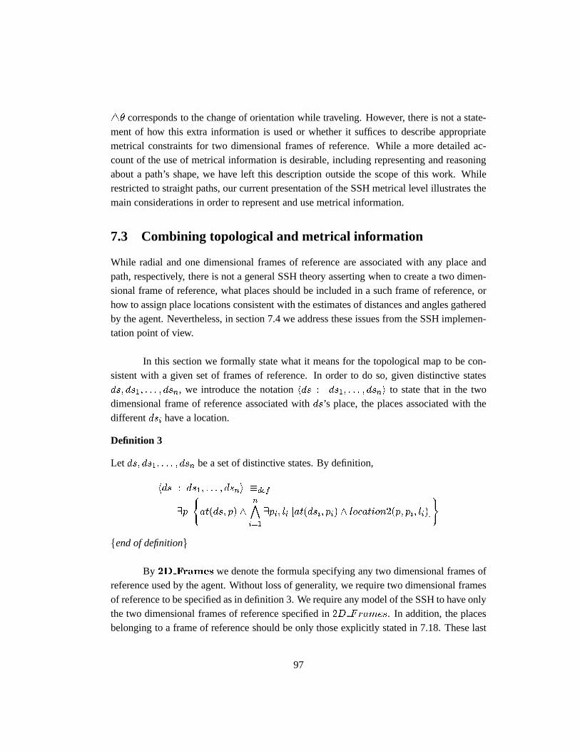
4� corresponds to the change of orientation while traveling. However, there is not a state-ment of how this extra information is used or whether it suffices to describe appropriatemetrical constraints for two dimensional frames of reference. While a more detailed ac-count of the use of metrical information is desirable, including representing and reasoningabout a path’s shape, we have left this description outside the scope of this work. Whilerestricted to straight paths, our current presentation of the SSH metrical level illustrates themain considerations in order to represent and use metrical information.

7.3 Combining topological and metrical information

While radial and one dimensional frames of reference are associated with any place andpath, respectively, there is not a general SSH theory asserting when to create a two dimen-sional frame of reference, what places should be included in a such frame of reference, orhow to assign place locations consistent with the estimates of distances and angles gatheredby the agent. Nevertheless, in section 7.4 we address these issues from the SSH implemen-tation point of view.

In this section we formally state what it means for the topological map to be con-sistent with a given set of frames of reference. In order to do so, given distinctive statesds; ds1; : : : ; dsn, we introduce the notationhds : ds1; : : : ; dsni to state that in the twodimensional frame of reference associated withds’s place, the places associated with thedifferentdsi have a location.

Definition 3

Let ds; ds1; : : : ; dsn be a set of distinctive states. By definition,

hds : ds1; : : : ; dsni �def

9p

(at(ds; p) ^

n

i=1

9pi; li [at(dsi; pi) ^ location2(p; pi; li)]

)

fend of definitiong

By 2D Frames we denote the formula specifying any two dimensional frames ofreference used by the agent. Without loss of generality, we require two dimensional framesof reference to be specified as in definition 3. We require any model of the SSH to have onlythe two dimensional frames of reference specified in2D Frames. In addition, the placesbelonging to a frame of reference should be only those explicitly stated in 7.18. These last

97

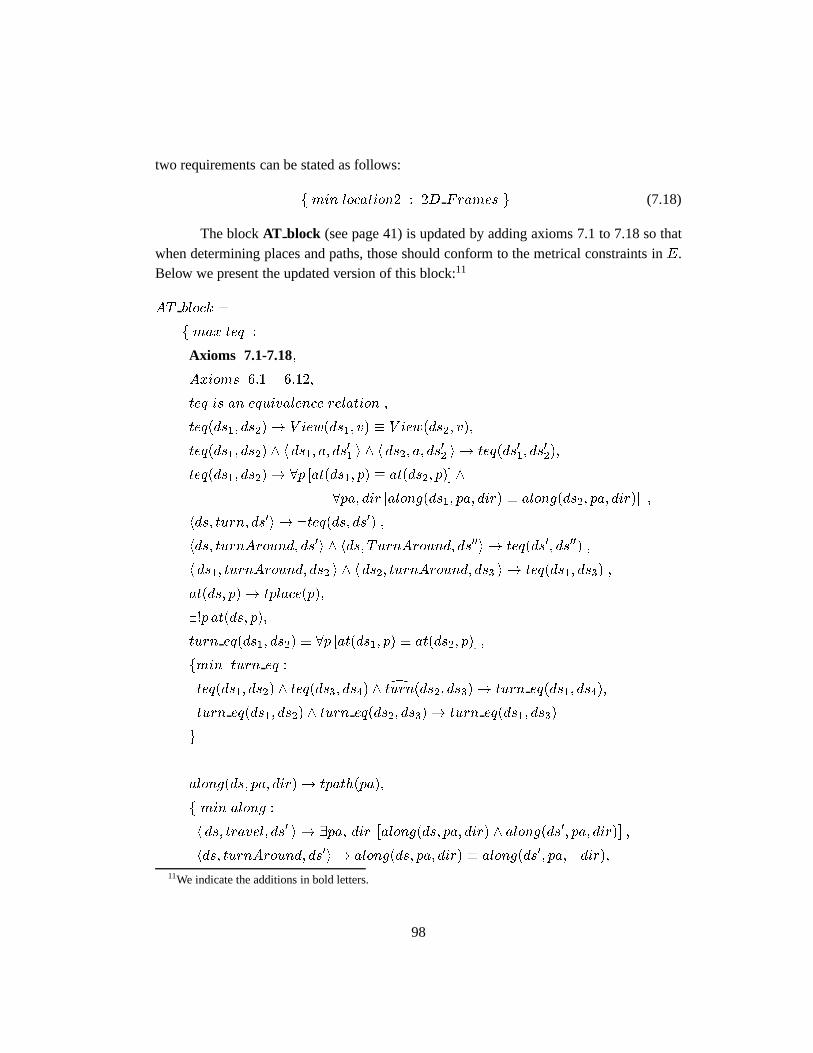
two requirements can be stated as follows:

f min location2 : 2D Frames g (7.18)

The blockAT block (see page 41) is updated by adding axioms 7.1 to 7.18 so thatwhen determining places and paths, those should conform to the metrical constraints inE.Below we present the updated version of this block:11

AT block =

f max teq :

Axioms 7.1-7.18;

Axioms 6:1� 6:12;

teq is an equivalence relation ;

teq(ds1; ds2)! V iew(ds1; v) � V iew(ds2; v);

teq(ds1; ds2) ^ h ds1; a; ds01 i ^ h ds2; a; ds

02 i ! teq(ds01; ds

02);

teq(ds1; ds2)! 8p [at(ds1; p) � at(ds2; p)] ^

8pa; dir [along(ds1; pa; dir) � along(ds2; pa; dir)] ;

hds; turn; ds0i ! :teq(ds; ds0) ;

hds; turnAround; ds0i ^ hds; TurnAround; ds00i ! teq(ds0; ds00) ;

h ds1; turnAround; ds2 i ^ h ds2; turnAround; ds3 i ! teq(ds1; ds3) ;

at(ds; p)! tplace(p);

9!p at(ds; p);

turn eq(ds1; ds2) � 8p [at(ds1; p) � at(ds2; p)] ;

fmin turn eq :

teq(ds1; ds2) ^ teq(ds3; ds4) ^ dturn(ds2; ds3)! turn eq(ds1; ds4);

turn eq(ds1; ds2) ^ turn eq(ds2; ds3)! turn eq(ds1; ds3)

g

along(ds; pa; dir)! tpath(pa);

f min along :

h ds; travel; ds0 i ! 9pa; dir�along(ds; pa; dir) ^ along(ds0; pa; dir)

�;

hds; turnAround; ds0i ! along(ds; pa; dir) � along(ds0; pa;�dir);

11We indicate the additions in bold letters.

98

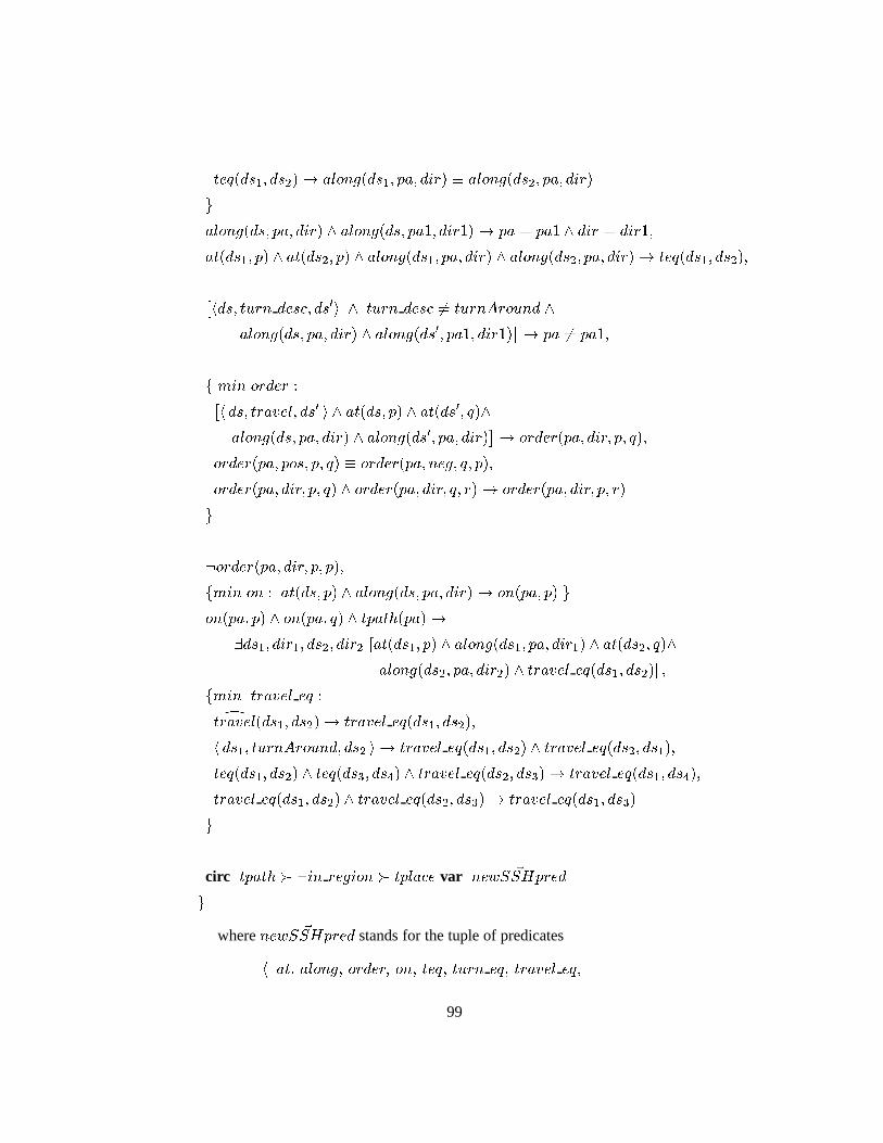
teq(ds1; ds2)! along(ds1; pa; dir) � along(ds2; pa; dir)

g

along(ds; pa; dir) ^ along(ds; pa1; dir1) ! pa = pa1 ^ dir = dir1;

at(ds1; p) ^ at(ds2; p) ^ along(ds1; pa; dir) ^ along(ds2; pa; dir)! teq(ds1; ds2);

�hds; turn desc; ds0i ^ turn desc 6= turnAround ^

along(ds; pa; dir) ^ along(ds0; pa1; dir1)�! pa 6= pa1;

f min order :�h ds; travel; ds0 i ^ at(ds; p) ^ at(ds0; q)^

along(ds; pa; dir) ^ along(ds0; pa; dir)�! order(pa; dir; p; q);

order(pa; pos; p; q) � order(pa; neg; q; p);

order(pa; dir; p; q) ^ order(pa; dir; q; r)! order(pa; dir; p; r)

g

:order(pa; dir; p; p);

fmin on : at(ds; p) ^ along(ds; pa; dir)! on(pa; p) g

on(pa; p) ^ on(pa; q) ^ tpath(pa)!

9ds1; dir1; ds2; dir2 [at(ds1; p) ^ along(ds1; pa; dir1) ^ at(ds2; q)^

along(ds2; pa; dir2) ^ travel eq(ds1; ds2)] ;

fmin travel eq :dtravel(ds1; ds2)! travel eq(ds1; ds2);

h ds1; turnAround; ds2 i ! travel eq(ds1; ds2) ^ travel eq(ds2; ds1);

teq(ds1; ds2) ^ teq(ds3; ds4) ^ travel eq(ds2; ds3)! travel eq(ds1; ds4);

travel eq(ds1; ds2) ^ travel eq(ds2; ds3)! travel eq(ds1; ds3)

g

circ tpath � :in region � tplace var ~newSSHpred

g

where ~newSSHpred stands for the tuple of predicates

h at; along; order; on; teq; turn eq; travel eq;

99

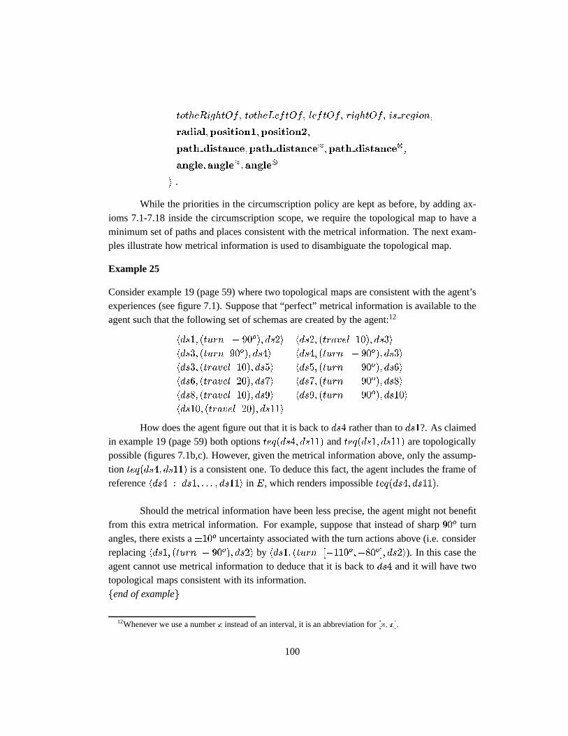
totheRightOf; totheLeftOf; leftOf; rightOf; is region;

radial;position1;position2;

path distance;path distance�;path distance;

angle;angle�;angle

i :

While the priorities in the circumscription policy are kept as before, by adding ax-ioms 7.1-7.18 inside the circumscription scope, we require the topological map to have aminimum set of paths and places consistent with the metrical information. The next exam-ples illustrate how metrical information is used to disambiguate the topological map.

Example 25

Consider example 19 (page 59) where two topological maps are consistent with the agent’sexperiences (see figure 7.1). Suppose that “perfect” metrical information is available to theagent such that the following set of schemas are created by the agent:12

hds1; (turn � 90o); ds2i hds2; (travel 10); ds3i

hds3; (turn 90o); ds4i hds4; (turn � 90o); ds3i

hds3; (travel 10); ds5i hds5; (turn � 90o); ds6i

hds6; (travel 20); ds7i hds7; (turn � 90o); ds8i

hds8; (travel 10); ds9i hds9; (turn � 90o); ds10i

hds10; (travel 20); ds11i

How does the agent figure out that it is back tods4 rather than tods1?. As claimedin example 19 (page 59) both optionsteq(ds4; ds11) andteq(ds1; ds11) are topologicallypossible (figures 7.1b,c). However, given the metrical information above, only the assump-tion teq(ds4; ds11) is a consistent one. To deduce this fact, the agent includes the frame ofreferencehds4 : ds1; : : : ; ds11i in E, which renders impossibleteq(ds4; ds11).

Should the metrical information have been less precise, the agent might not benefitfrom this extra metrical information. For example, suppose that instead of sharp90o turnangles, there exists a�10o uncertainty associated with the turn actions above (i.e. considerreplacinghds1; (turn � 90o); ds2i by hds1; (turn [�110o;�80o]; ds2i). In this case theagent cannot use metrical information to deduce that it is back tods4 and it will have twotopological maps consistent with its information.fend of exampleg

12Whenever we use a numberx instead of an interval, it is an abbreviation for[x; x].

100

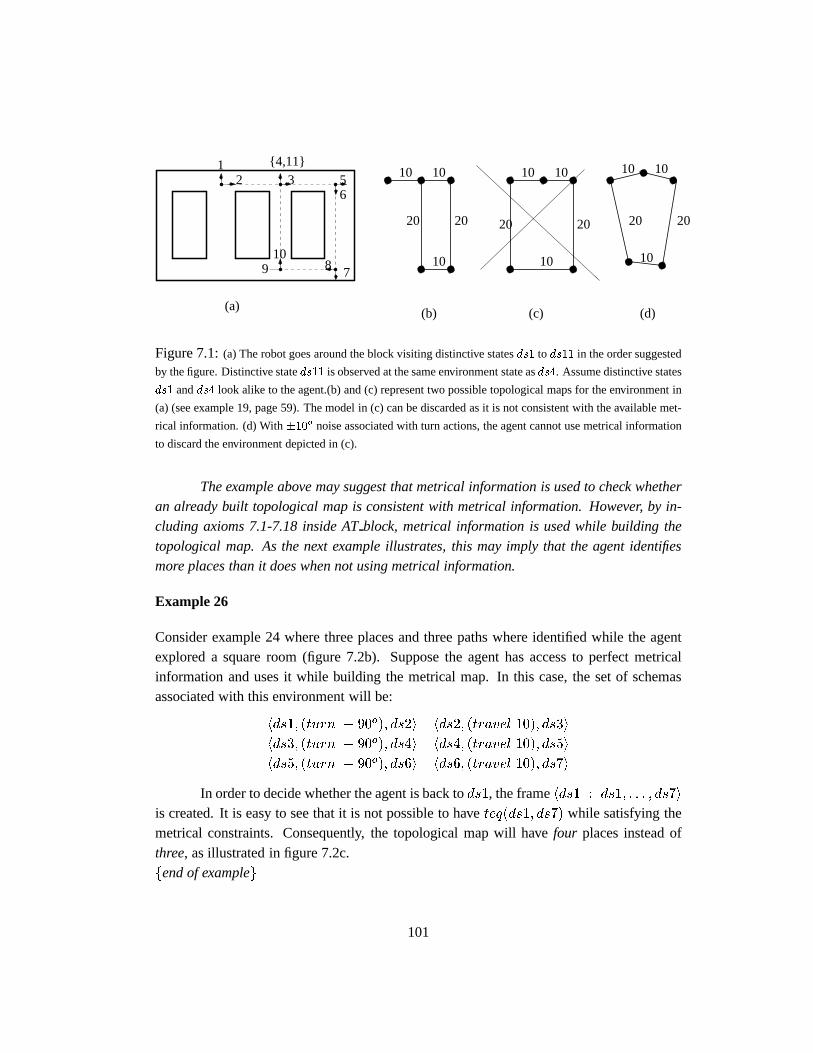
(a)

10

20

1010

2020

1010

20

107

6

{4,11}

8910

1532

(d)(c)(b)

10

20

1010

20

Figure 7.1:(a) The robot goes around the block visiting distinctive statesds1 to ds11 in the order suggested

by the figure. Distinctive stateds11 is observed at the same environment state asds4. Assume distinctive states

ds1 andds4 look alike to the agent.(b) and (c) represent two possible topological maps for the environment in

(a) (see example 19, page 59). The model in (c) can be discarded as it is not consistent with the available met-

rical information. (d) With�10o noise associated with turn actions, the agent cannot use metrical information

to discard the environment depicted in (c).

The example above may suggest that metrical information is used to check whetheran already built topological map is consistent with metrical information. However, by in-cluding axioms 7.1-7.18 inside ATblock, metrical information is used while building thetopological map. As the next example illustrates, this may imply that the agent identifiesmore places than it does when not using metrical information.

Example 26

Consider example 24 where three places and three paths where identified while the agentexplored a square room (figure 7.2b). Suppose the agent has access to perfect metricalinformation and uses it while building the metrical map. In this case, the set of schemasassociated with this environment will be:

hds1; (turn � 90o); ds2i hds2; (travel 10); ds3i

hds3; (turn � 90o); ds4i hds4; (travel 10); ds5i

hds5; (turn � 90o); ds6i hds6; (travel 10); ds7i

In order to decide whether the agent is back tods1, the framehds1 : ds1; : : : ; ds7i

is created. It is easy to see that it is not possible to haveteq(ds1; ds7) while satisfying themetrical constraints. Consequently, the topological map will havefour places instead ofthree, as illustrated in figure 7.2c.fend of exampleg

101

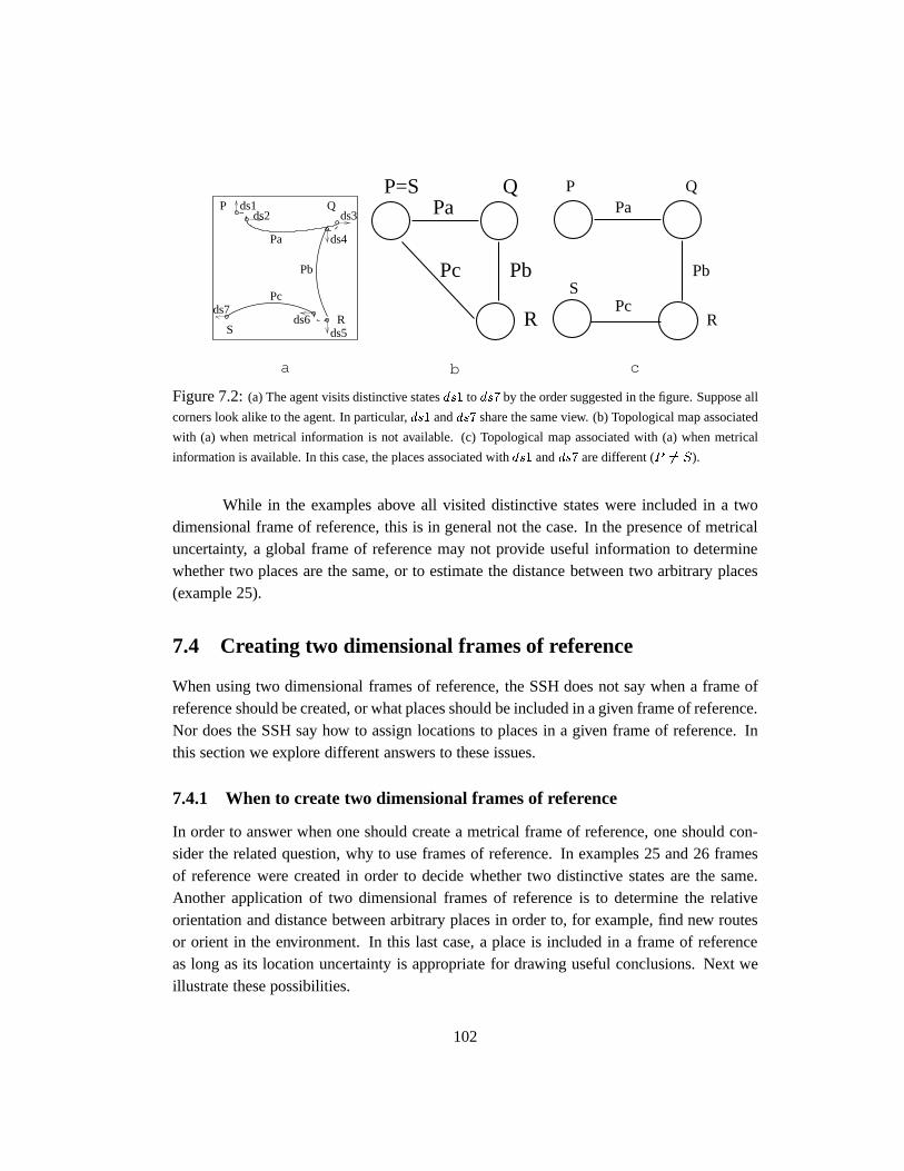
ds7

S

ds2ds1P

ds3

ds6ds5

R

Pc

Pa

Pb

ds4

Q

R

Pb

QPa

P=S

Pc

Q

R

Pa

Pb

P

SPc

a b c

Figure 7.2:(a) The agent visits distinctive statesds1 to ds7 by the order suggested in the figure. Suppose all

corners look alike to the agent. In particular,ds1 andds7 share the same view. (b) Topological map associated

with (a) when metrical information is not available. (c) Topological map associated with (a) when metrical

information is available. In this case, the places associated withds1 andds7 are different (P 6= S).

While in the examples above all visited distinctive states were included in a twodimensional frame of reference, this is in general not the case. In the presence of metricaluncertainty, a global frame of reference may not provide useful information to determinewhether two places are the same, or to estimate the distance between two arbitrary places(example 25).

7.4 Creating two dimensional frames of reference

When using two dimensional frames of reference, the SSH does not say when a frame ofreference should be created, or what places should be included in a given frame of reference.Nor does the SSH say how to assign locations to places in a given frame of reference. Inthis section we explore different answers to these issues.

7.4.1 When to create two dimensional frames of reference

In order to answer when one should create a metrical frame of reference, one should con-sider the related question, why to use frames of reference. In examples 25 and 26 framesof reference were created in order to decide whether two distinctive states are the same.Another application of two dimensional frames of reference is to determine the relativeorientation and distance between arbitrary places in order to, for example, find new routesor orient in the environment. In this last case, a place is included in a frame of referenceas long as its location uncertainty is appropriate for drawing useful conclusions. Next weillustrate these possibilities.

102

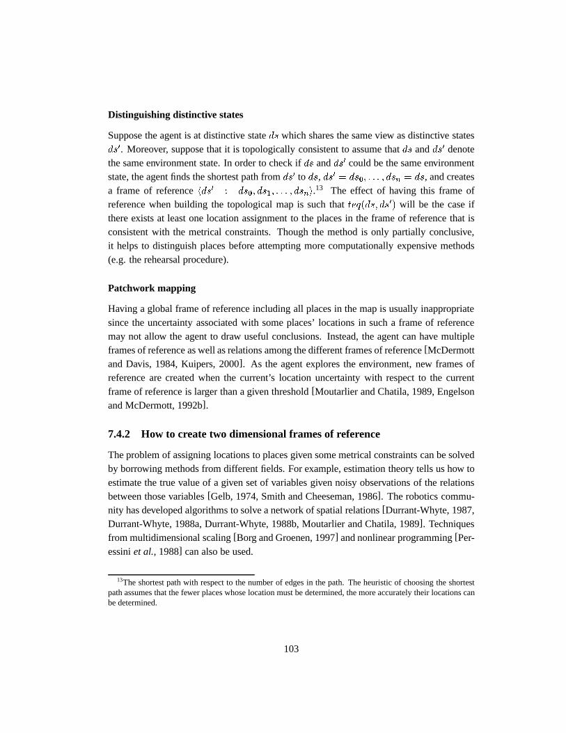
Distinguishing distinctive states

Suppose the agent is at distinctive stateds which shares the same view as distinctive statesds0. Moreover, suppose that it is topologically consistent to assume thatds andds0 denotethe same environment state. In order to check ifds andds0 could be the same environmentstate, the agent finds the shortest path fromds0 to ds, ds0 = ds0; : : : ; dsn = ds, and createsa frame of referencehds0 : ds0; ds1; : : : ; dsni.13 The effect of having this frame ofreference when building the topological map is such thatteq(ds; ds0) will be the case ifthere exists at least one location assignment to the places in the frame of reference that isconsistent with the metrical constraints. Though the method is only partially conclusive,it helps to distinguish places before attempting more computationally expensive methods(e.g. the rehearsal procedure).

Patchwork mapping

Having a global frame of reference including all places in the map is usually inappropriatesince the uncertainty associated with some places’ locations in such a frame of referencemay not allow the agent to draw useful conclusions. Instead, the agent can have multipleframes of reference as well as relations among the different frames of reference[McDermottand Davis, 1984, Kuipers, 2000]. As the agent explores the environment, new frames ofreference are created when the current’s location uncertainty with respect to the currentframe of reference is larger than a given threshold[Moutarlier and Chatila, 1989, Engelsonand McDermott, 1992b].

7.4.2 How to create two dimensional frames of reference

The problem of assigning locations to places given some metrical constraints can be solvedby borrowing methods from different fields. For example, estimation theory tells us how toestimate the true value of a given set of variables given noisy observations of the relationsbetween those variables[Gelb, 1974, Smith and Cheeseman, 1986]. The robotics commu-nity has developed algorithms to solve a network of spatial relations[Durrant-Whyte, 1987,Durrant-Whyte, 1988a, Durrant-Whyte, 1988b, Moutarlier and Chatila, 1989]. Techniquesfrom multidimensional scaling[Borg and Groenen, 1997] and nonlinear programming[Per-essiniet al., 1988] can also be used.

13The shortest path with respect to the number of edges in the path. The heuristic of choosing the shortestpath assumes that the fewer places whose location must be determined, the more accurately their locations canbe determined.

103

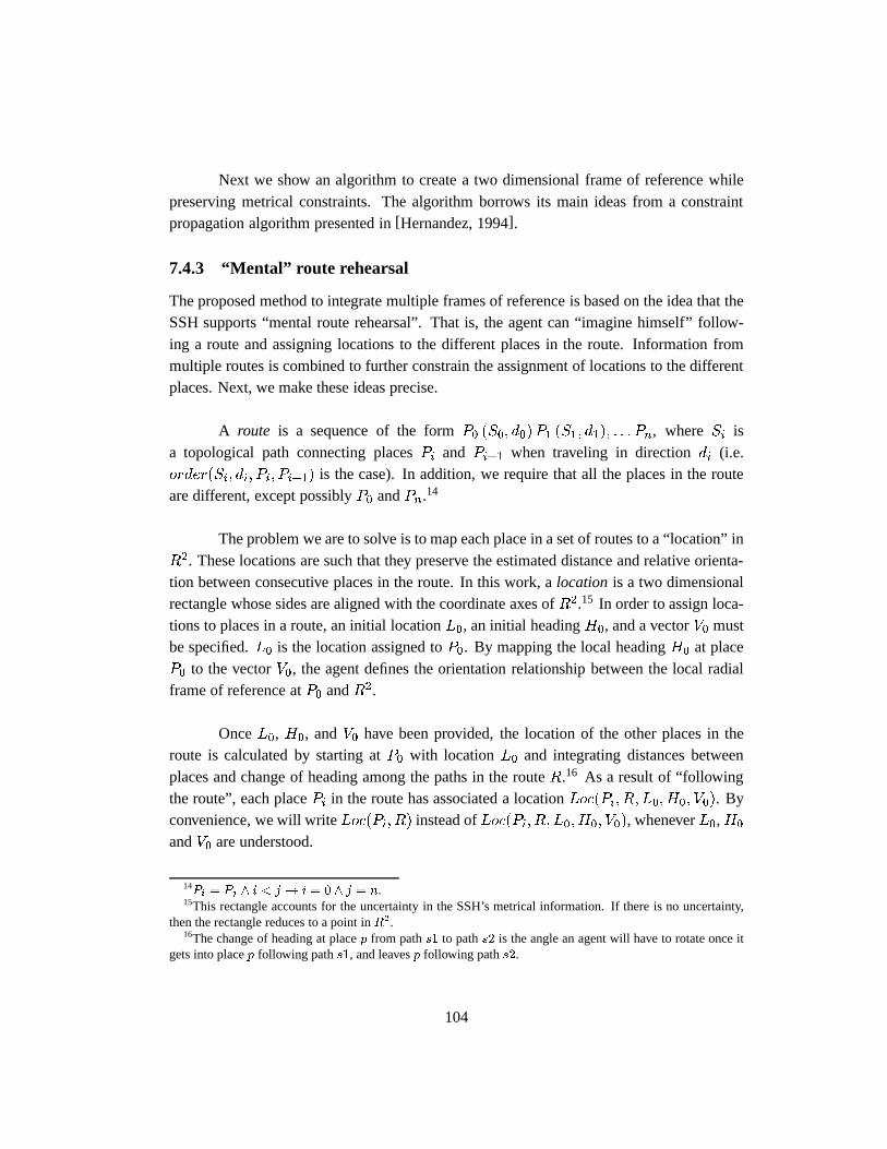
Next we show an algorithm to create a two dimensional frame of reference whilepreserving metrical constraints. The algorithm borrows its main ideas from a constraintpropagation algorithm presented in[Hernandez, 1994].

7.4.3 “Mental” route rehearsal

The proposed method to integrate multiple frames of reference is based on the idea that theSSH supports “mental route rehearsal”. That is, the agent can “imagine himself” follow-ing a route and assigning locations to the different places in the route. Information frommultiple routes is combined to further constrain the assignment of locations to the differentplaces. Next, we make these ideas precise.

A route is a sequence of the formP0 (S0; d0)P1 (S1; d1); : : : Pn, whereSi isa topological path connecting placesPi and Pi+1 when traveling in directiondi (i.e.order(Si; di; Pi; Pi+1) is the case). In addition, we require that all the places in the routeare different, except possiblyP0 andPn.14

The problem we are to solve is to map each place in a set of routes to a “location” inR2. These locations are such that they preserve the estimated distance and relative orienta-tion between consecutive places in the route. In this work, alocation is a two dimensionalrectangle whose sides are aligned with the coordinate axes ofR2.15 In order to assign loca-tions to places in a route, an initial locationL0, an initial headingH0, and a vectorV0 mustbe specified.L0 is the location assigned toP0. By mapping the local headingH0 at placeP0 to the vectorV0, the agent defines the orientation relationship between the local radialframe of reference atP0 andR2.

OnceL0, H0, andV0 have been provided, the location of the other places in theroute is calculated by starting atP0 with locationL0 and integrating distances betweenplaces and change of heading among the paths in the routeR.16 As a result of “followingthe route”, each placePi in the route has associated a locationLoc(Pi; R; L0;H0; V0). Byconvenience, we will writeLoc(Pi; R) instead ofLoc(Pi; R; L0;H0; V0), wheneverL0,H0

andV0 are understood.

14Pi = Pj ^ i < j ! i = 0 ^ j = n.15This rectangle accounts for the uncertainty in the SSH’s metrical information. If there is no uncertainty,

then the rectangle reduces to a point inR2.16The change of heading at placep from paths1 to paths2 is the angle an agent will have to rotate once it

gets into placep following paths1, and leavesp following paths2.

104

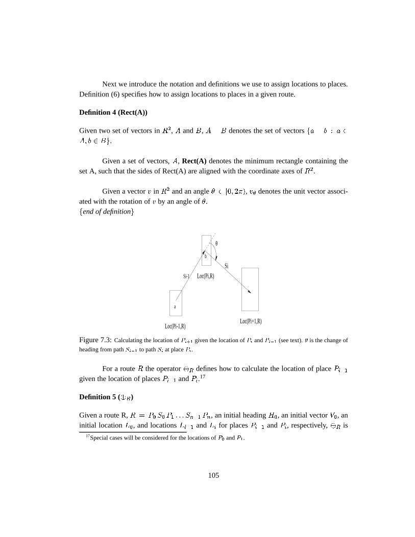
Next we introduce the notation and definitions we use to assign locations to places.Definition (6) specifies how to assign locations to places in a given route.

Definition 4 (Rect(A))

Given two set of vectors inR2, A andB, A + B denotes the set of vectorsfa + b : a 2

A; b 2 Bg.

Given a set of vectors,A, Rect(A) denotes the minimum rectangle containing theset A, such that the sides of Rect(A) are aligned with the coordinate axes ofR2.

Given a vectorv in R2 and an angle� 2 [0; 2�), v� denotes the unit vector associ-ated with the rotation ofv by an angle of�.fend of definitiong

a

b

θ

Loc(Pi-1,R)

Loc(Pi,R)

Loc(Pi+1,R)

Si-1

Si

Figure 7.3:Calculating the location ofPi+1 given the location ofPi andPi�1 (see text).� is the change of

heading from pathSi�1 to pathSi at placePi.

For a routeR the operator�R defines how to calculate the location of placePi+1

given the location of placesPi�1 andPi.17

Definition 5 (�R)

Given a route R,R = P0 S0 P1 : : : Sn�1 Pn, an initial headingH0, an initial vectorV0, aninitial locationL0, and locationsLi�1 andLi for placesPi�1 andPi, respectively,�R is

17Special cases will be considered for the locations ofP0 andP1.

105

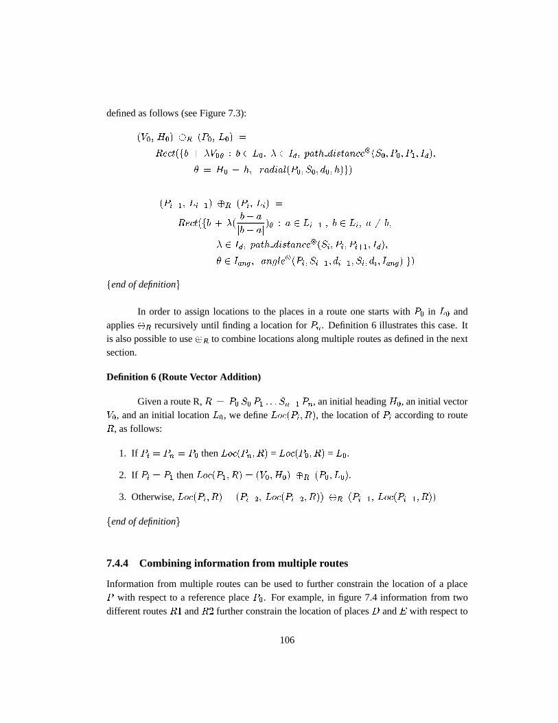
defined as follows (see Figure 7.3):

(V0; H0) �R (P0; L0) =

Rect(fb + �V0� : b 2 L0; � 2 Id; path distance(S0; P0; P1; Id);

� = H0 � h; radial(P0; S0; d0; h)g)

(Pi�1; Li�1) �R (Pi; Li) =

Rect(fb + �(b� a

jb� aj)� : a 2 Li�1 ; b 2 Li; a 6= b;

� 2 Id; path distance(Si; Pi; Pi+1; Id);

� 2 Iang; angle(Pi; Si�1; di�1; Si; di; Iang) g)

fend of definitiong

In order to assign locations to the places in a route one starts withP0 in L0 andapplies�R recursively until finding a location forPn. Definition 6 illustrates this case. Itis also possible to use�R to combine locations along multiple routes as defined in the nextsection.

Definition 6 (Route Vector Addition)

Given a route R,R = P0 S0 P1 : : : Sn�1 Pn, an initial headingH0, an initial vectorV0, and an initial locationL0, we defineLoc(Pi; R), the location ofPi according to routeR, as follows:

1. If Pi = Pn = P0 thenLoc(Pn; R) = Loc(P0; R) = L0.

2. If Pi = P1 thenLoc(P1; R) = (V0;H0) �R (P0; L0).

3. Otherwise,Loc(Pi; R) = (Pi�2; Loc(Pi�2; R)) �R (Pi�1; Loc(Pi�1; R))

fend of definitiong

7.4.4 Combining information from multiple routes

Information from multiple routes can be used to further constrain the location of a placeP with respect to a reference placeP0. For example, in figure 7.4 information from twodifferent routesR1 andR2 further constrain the location of placesD andE with respect to

106

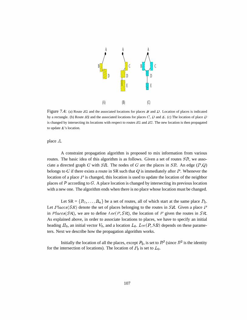
(A) (B) (C)

E

D

A

B

A

D

B

A

C

D

E

C

���������

���������

������������

������������

��������

��������

������������

������������

����������

������������

������

Figure 7.4:(a) RouteR1 and the associated locations for placesB andD. Location of places is indicated

by a rectangle. (b) RouteR2 and the associated locations for placesC, D andE. (c) The location of placeD

is changed by intersecting its locations with respect to routesR1 andR2. The new location is then propagated

to updateE’s location.

placeA.

A constraint propagation algorithm is proposed to mix information from variousroutes. The basic idea of this algorithm is as follows. Given a set of routesSR, we asso-ciate a directed graphG with SR. The nodes ofG are the places inSR. An edge (P ,Q)belongs toG if there exists a route in SR such thatQ is immediately afterP . Whenever thelocation of a placeP is changed, this location is used to update the location of the neighborplaces ofP according toG. A place location is changed by intersecting its previous locationwith a new one. The algorithm ends when there is no place whose location must be changed.

Let SR =fR1; : : : ; Rng be a set of routes, all of which start at the same placeP0.Let P laces(SR) denote the set of places belonging to the routes inSR. Given a placePin P laces(SR), we are to defineLoc(P; SR), the location ofP given the routes inSR.As explained above, in order to associate locations to places, we have to specify an initialheadingH0, an initial vectorV0, and a locationL0. Loc(P; SR) depends on these parame-ters. Next we describe how the propagation algorithm works.

Initially the location of all the places, exceptP0, is set toR2 (sinceR2 is the identityfor the intersection of locations). The location ofP0 is set toL0.

107

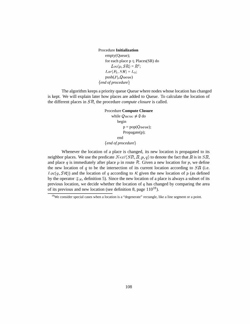
ProcedureInitializationempty(Queue);for each place p2 Places(SR) do

Loc(p; SR) = R2;Loc(P0; SR) = L0;push(P0,Queue)

fend of procedureg

The algorithm keeps a priority queueQueuewhere nodes whose location has changedis kept. We will explain later how places are added toQueue. To calculate the location ofthe different places inSR, the procedurecompute closureis called.

ProcedureCompute ClosurewhileQueue 6= ; do

beginp = pop(Queue);Propagate(p);

endfend of procedureg

Whenever the location of a place is changed, its new location is propagated to itsneighbor places. We use the predicateNext(SR;R; p; q) to denote the fact thatR is inSR,and placeq is immediately after placep in routeR. Given a new location forp, we definethe new location ofq to be the intersection of its current location according toSR (i.e.Loc(q; SR)) and the location ofq according toR given the new location ofp (as definedby the operator�R, definition 5). Since the new location of a place is always a subset of itsprevious location, we decide whether the location ofq has changed by comparing the areaof its previous and new location (see definition 8, page 11018).

18We consider special cases when a location is a “degenerate” rectangle, like a line segment or a point.

108

ProcedurePropagate (p)for each placeq such thatNext(SR;R; p; q) do

beginif 9p0; (p0; p; R)

then New :=Loc(q; SR) \ (p0; Loc(r; SR)�R (p; Loc(p; SR))

else New :=Loc(q; SR) \ (V0; H0)�R (p; Loc(p; SR))

if New = ;then signal contradictionif Change(New,Loc(q; SR))

thenbegin

add q toQueueLoc(q; SR) := New

endend

fend of procedureg

The next example illustrates how the algorithm works to combine the informationfrom the routes in figure 7.4.

Example 27

Consider the routesR1 andR2 depicted in figure 7.4. We start the algorithm by calling theprocedure initialization, after which we have that19

Loc(A) = {(0,0)}, Loc(B) = Loc(C) = Loc(D) = Loc(E) = Rˆ2Queue = [A]

The procedure Compute Closure is then invoked, A is removed fromQueue, and the proce-durePropagate(A) is called. New locations for placesB andC are then calculated. Thenew locations become:

Loc(A) = {(0,0)}, Loc(B) = L1, Loc (C) = L2, Loc(D)=Loc(E) = Rˆ2

Queue = [B,C]

whereL1 andL2 are the locations calculated forB andC respectively. NowB is takenfrom QueueandPropagate(B) is called, after which we have that

Loc(A) = {(0,0)}, Loc(B)= L1, Loc (C)= L2, Loc(D)= L3, Loc(E) = Rˆ2Queue = [C,D]

Propagate(C) will be called and the location ofD is changed by intersecting informationfrom both routes,

19We will omit the parameterSR in Loc(p; SR) and writeLoc(p).

109

Loc(A) = {(0,0)}, Loc(B) = L1, Loc (C) = L2, Loc(D)= L3 inter L3’

Loc(E) = Rˆ2

Queue = [D]

L3 and L3’ are the location ofD according to routeR1 andR2, respectively. Finally,Propagate(D) is called which will give a value for the location ofE.fend of exampleg

In the example above, we did not propagate the location of any place twice. Ingeneral this is not the case, and we need to be more strict on how places are taken fromQueue whenPropagate is called. In order to do so, we impose an order,beforeSR(p; q),among the places inSR. Next we definebeforeSR(p; q).

Definition 7 (beforeSR(p; q))

Given a set of routesSR, placesp andq in P laces(SR), we say that placep is before placeq according toSR, beforeSR(p; q), if (i) there exists a routeR in SR such thatp is beforeq in R, and (ii) there does not exist a routeR in SR such thatq is beforep in R.fend of definitiong

The relationbeforeSR defines a partial order among the places inSR. We use it toprioritize the places in Queue, such that wheneverbeforeSR(p; q) is the case, the priorityof p is greater than the priority ofq.

In order to decide whether the location of a place has changed, we compare theareas between the new and the old place location, as stated in the next definition.

Definition 8 (Change(new,old))

Given two locations,new andold, such thatnew � old, change(new,old)is true if andonly if one of the following conditions is true

1. old =R2 and new6= R2.

2. both old and new are rectangles and[area(old) � area(new)] > �, for a given� > 0.

3. old is a rectangle and new is a line segment or a point.

4. both old and new are line segments and[length(old) � length(new)] > �, for agiven� > 0.

110

5. old is not a point and new is a point.

fend of definitiong

The proposed algorithm assigns locations to places in a “liberal” way.20 By choos-ing an arbitrary point from a place’s location as the actual place position, the resulting as-signment of positions does not necessarily satisfy the distance and angle constraints amongplaces. However, any assignment of places’ positions satisfying these constraints is cov-ered by the places’ locations produced by our algorithm. Should the application at handrequire such assignment of positions, starting from the locations assigned by our algorithmone could use Monte Carlo or hill-climbing algorithms to find such assignment (if exists)[McDermott and Davis, 1984].

Possible applications of our algorithm include answering queries about the spatiallayout and visualization of the topological map:

� Answering some queries about the spatial layout can be rendered to check some prop-erties in the location assigned to places. For example, to answer whether placeA isto the left or right of placeB, when facing heading� atB, the following procedureis used. Find a route fromB to A. Let P0 beB, H0 = � andV0 = (0; 1). A is tothe left of B if the location ofA is contained inf(x; y) : x < 0)g. A is to the rightof B if the location ofA is contained inf(x; y) : x > 0)g. Otherwise the agent doesnot decide whetherA is to the left or right ofB. Notice that given the uncertaintyassociated with distances and angles, the proposed method is partially conclusive: itcould answeryes, noor maybe.

� Displaying the layout of places in a computer screen is important for a robot-humaninterface. Having pre-defined two dimensional frames of reference allows one toquickly display a region or neighborhood, a display that is useful for specifying nav-igation goals as well as generating explanations of the robot’s navigation plans.

7.5 Summary

In this chapter we have defined different kinds of frames of reference considered in theSSH: one dimensional frames of reference which assign positions to places on a path, ra-dial frames of reference that assign angles to the different paths that intersect at a given

20We borrow this term from[McDermott and Davis, 1984]. In a “liberal” map, the location of places grantsas much freedom as possible to each place even though not every coordinates we pick within a place locationwill satisfy all metrical constraints. This would be the case in a “conservative” map.

111

place, and two dimensional frames of reference which assign positions to arbitrary set ofplaces. Our formalization describes how uncertainty associated with metrical informationis taken into account when creating these frames of reference. In particular, we have de-scribed how to represent different metrical measurement estimates, how to combine them,and how to represent the constraints they impose on the metrical relations among differentobjects referenced by a frame of reference.

Uncertainty in metrical information has been represented by one and two dimen-sional rectangles. This representation is adequate for most practical uses. However, moresophisticated representations of uncertainty are compatible with our methods. For example,probability density functions (such as Gaussians) can be used to represent uncertainty onthe distances between places in a path.

The SSH theory does not specify when to create two dimensional frames of refer-ence. We have described particular instances when this should be done: in order to disam-biguate places or when uncertainty in a place location is “high”. Given that the actual formaltreatment of uncertainty propagation is outside the scope of this work, we have providedpointers to the relevant fields where such studies are done (see section 7.4.1). Nevertheless,we have described a constraint propagation algorithm to integrate multiple frames of ref-erence while assigning locations to places in a given set of routes. Locations are assignedsuch that they preserve the estimated distance and relative orientation between consecutiveplaces in a path (see section 7.4.3).

Finally, we have pointed out that our current description of two dimensional framesof reference assumes environments where paths are straight. Nevertheless, our current pre-sentation of the SSH metrical level illustrates the main considerations in order to representand use metrical information. A more detailed account of the use of metrical information,possibly by reasoning about the shape of paths, is suggested as future work.

112

Chapter 8

Regions

As the agent explores its environment, the number of places it identifies grows. Conse-quently, the topological map, as described until now, might have so much information thatit will be cumbersome (i.e. time-consuming) to use for future navigation or for a humanlevel interface.1 It is useful then to define a hierarchical representation that simplifies somedetails in the topological map. The basic abstraction method we use is to groupplaces intoregions. As for topological places, regions are ordered along routes, and in turn they can begrouped to form new regions, giving the representation a powerful mechanism of abstrac-tion. Metrical information about regions, like their distance along a route or their relativedirection, can be derived from the corresponding metrical relations among the places in theregions. In this chapter we state how to represent regions in the SSH as well as the prop-erties of the hierarchical representation associated with them. We also illustrate the use ofregions for hierarchical planning and qualitative reasoning about space.2 Finally, we alsoprovide some criteria for automatically identifying regions and creating their associatedhierarchy.

8.1 Including regions in the SSH topological level

Regions are sets of places.Regions themselves can be grouped to form new regions.Since regions can be seen as places, we have not added a new sortregions to the SSH

1Similar problem occurs when a QSIM behavior graph has many states. A way to simplify these behaviorsgraphs is to abstract together adjacent states that, by according to a user’s criteria, need not be distinguished[Mallory et al., 1996].

2Further uses of regions can be found in section A.3, page 209 (hierarchical plan execution).

113

topological level ontology. We use the predicate3

in region(p; r)

to denote thatplacep is in region r. Recall that the sort of places contains the subsorts oftopological paths and regions. In chapter 5 we required that (see axiom 5.4, page 39)

:9p [tplace(p) ^ is region(p)]

wherep is a variable taking values in the sort ofplaces. Similarly, in chapter 6 we restrictedthe domain ofin regionsuch that (see axiom 6.6, page 80)

in region(p; r)! is region(r) :

We require that the transitive closure ofin region defines a DAG4. Formally, werestrict our attention to models of the following formulae:

:in region�(r; r);

f min in region� :

in region(p; r)! in region�(p; r);

in region�(p; q) ^ in region�(q; r)! in region�(p; r)

g

where in region� denotes the transitive closure ofin region. Equality amongregions is defined as expected: two regions are equal whenever they represent the same setof places. Formally,

is region(r) ^ is region(r0)! r = r0 � 8p fin region�(p; r) � in region�(p; r0)g

Once places have been arranged into regions, we must define connectivity relationsamong them. We do so bylifting the order relation among places in a path to their corre-sponding regions. The next section presents how to do so.

8.1.1 Defining paths among regions

Recall that the sort of paths contains the subsorts of topological paths and routes, as statedby axiom 5.5 in chapter 5 (see page 39):

:9pa [tpath(pa) ^ route(pa)] ;3This predicate has been used in the previous chapters. Here we will define the minimum constraints on this

predicate.4Directed Acyclic Graph.

114

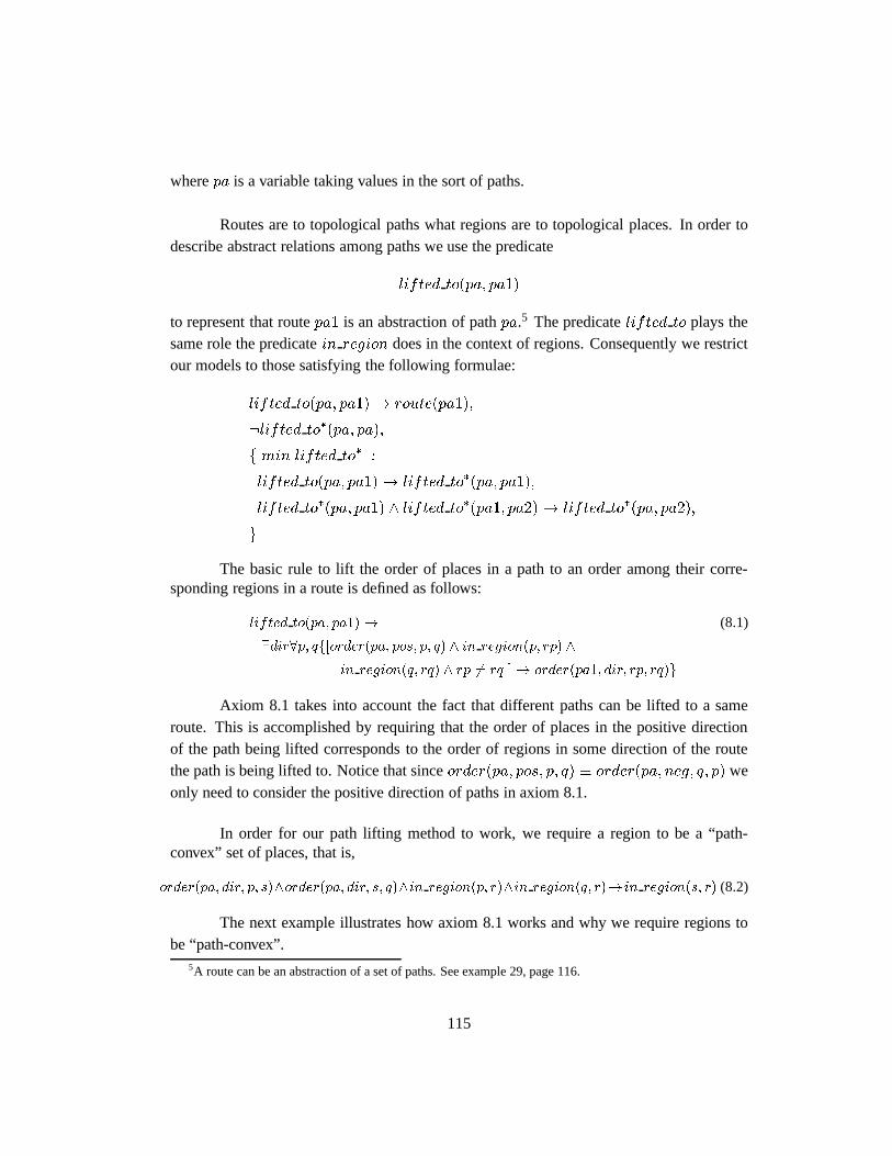
wherepa is a variable taking values in the sort of paths.

Routes are to topological paths what regions are to topological places. In order todescribe abstract relations among paths we use the predicate

lifted to(pa; pa1)

to represent that routepa1 is an abstraction of pathpa.5 The predicatelifted to plays thesame role the predicatein region does in the context of regions. Consequently we restrictour models to those satisfying the following formulae:

lifted to(pa; pa1)! route(pa1);

:lifted to�(pa; pa);

f min lifted to� :

lifted to(pa; pa1)! lifted to�(pa; pa1);

lifted to�(pa; pa1) ^ lifted to�(pa1; pa2)! lifted to�(pa; pa2);

g

The basic rule to lift the order of places in a path to an order among their corre-sponding regions in a route is defined as follows:

lifted to(pa; pa1)! (8.1)

9dir8p; qf[order(pa; pos; p; q) ^ in region(p; rp) ^

in region(q; rq) ^ rp 6= rq ]! order(pa1; dir; rp; rq)g

Axiom 8.1 takes into account the fact that different paths can be lifted to a sameroute. This is accomplished by requiring that the order of places in the positive directionof the path being lifted corresponds to the order of regions in some direction of the routethe path is being lifted to. Notice that sinceorder(pa; pos; p; q) � order(pa; neg; q; p) weonly need to consider the positive direction of paths in axiom 8.1.

In order for our path lifting method to work, we require a region to be a “path-convex” set of places, that is,

order(pa; dir; p; s)^order(pa; dir; s; q)^in region(p; r)^in region(q; r)! in region(s; r) (8.2)

The next example illustrates how axiom 8.1 works and why we require regions tobe “path-convex”.

5A route can be an abstraction of a set of paths. See example 29, page 116.

115

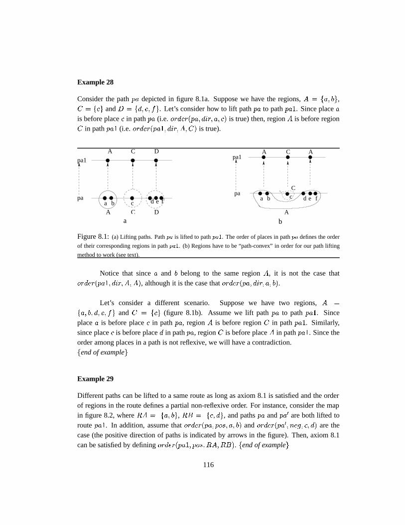
Example 28

Consider the pathpa depicted in figure 8.1a. Suppose we have the regions,A = fa; bg,C = fcg andD = fd; e; fg. Let’s consider how to lift pathpa to pathpa1. Since placeais before placec in pathpa (i.e. order(pa; dir; a; c) is true) then, regionA is before regionC in pathpa1 (i.e. order(pa1; dir; A;C) is true).

pa1

paa b c d e

A

f

C DA

C Dpa1

A C A

paa b c d e f

A

C

a b

Figure 8.1:(a) Lifting paths. Pathpa is lifted to pathpa1. The order of places in pathpa defines the order

of their corresponding regions in pathpa1. (b) Regions have to be “path-convex” in order for our path lifting

method to work (see text).

Notice that sincea and b belong to the same regionA, it is not the case thatorder(pa1; dir; A;A), although it is the case thatorder(pa; dir; a; b).

Let’s consider a different scenario. Suppose we have two regions,A =

fa; b; d; e; fg andC = fcg (figure 8.1b). Assume we lift pathpa to pathpa1. Sinceplacea is before placec in pathpa, regionA is before regionC in pathpa1. Similarly,since placec is before placed in pathpa, regionC is before placeA in pathpa1. Since theorder among places in a path is not reflexive, we will have a contradiction.fend of exampleg

Example 29

Different paths can be lifted to a same route as long as axiom 8.1 is satisfied and the orderof regions in the route defines a partial non-reflexive order. For instance, consider the mapin figure 8.2, whereRA = fa; bg, RB = fc; dg, and pathspa andpa0 are both lifted toroutepa1. In addition, assume thatorder(pa; pos; a; b) andorder(pa0; neg; c; d) are thecase (the positive direction of paths is indicated by arrows in the figure). Then, axiom 8.1can be satisfied by definingorder(pa1; pos;RA;RB). fend of exampleg

116

RA RB

pa1

pa

pa’dc

RA RB

a b

Figure 8.2:A route can be an abstraction of different paths.

The places at which a path enters or leaves a region are used to translate routesfrom one level of the hierarchy to actual behaviors at the SSH control level (page 118).This in turn implies that we can use hierarchical planning techniques when navigating theenvironment (see pages 207 and 209). The predicates

place enter(pa; dir; r; p); path leaves(pa; dir; r; p)

are used to denote thatp is a place at which the pathpa enters (leaves) regionr, whenfollowing pa in directiondir.6 We explicitly define these predicates as follows:

place enter(pa; dir; r; p)def� (8.3)

in region(p; r) ^ 8q forder(pa; dir; q; p)! :in region(q; r)g

place leaves(pa; dir; r; p)def� place enter(pa;�dir; r; p) (8.4)

The constraints imposed on the hierarchy of regions and paths do not excludebizarre structures. Moreover, different hierarchies can be implicitly represented by thepredicatein region. In practice, it is the case that one imposes more structure on theabstraction hierarchy. In particular, “stratified” hierarchies turn out to be the common ones:

Definition 9 (Stratified hierarchies)

The relationin region defines astratified hierarchyover a set of placesSH if there exista natural numbern, and a functionlevel from SH into f0; : : : ; ng such that:

1. p 2 SH ^ tplace(p)! level(p) = 0.

2. p 2 SH ^ r 2 SH ^ in region(p; r)! level(r) = level(p) + 1.

3. p 2 SH ^ q 2 SH ^ on(pa; p) ^ on(pa; q)! level(p) = level(q).6Given that the order of places is not necessarily a total order, there could exist different places at which a

path enters (leaves) a region.

117

4. r 2 SH ^ level(r) < n! 9r0 in region(r; r0).

In addition, we require regions to be connected

p 2 SH^r2SH^q2SH^in region(p; r)^in region(q; r)! connected(r; p; q) (8.5)

were the predicateconnected is such that

f min connected :

in region(p; r)! connected(r; p; p);

order(pa; dir; p; q) ^ in region(p; r) ^ in region(q; r)! connected(r; p; q);

connected(r; p; q) ^ connected(r; q; s)! connected(r; p; s)

g

fend of definitiong

Regions in a stratified hierarchy are connected sets of places, such that it shouldbe possible to go from one place to another in a region by only visiting places inside thatregion.7 The connectedness property will ensure that a route at any level of a stratifiedhierarchy has an associated route at level zero of the hierarchy. This property in turnsimplies that “navigation plans” described at different levels of detail can be translated toactual behavior. The actual behavior is found by repeatedly refining a route at levelk; k > 1,to a route at levelk � 1, until finding a route at level0. Next we define what a refinementfor a route is.

Notation 1

A route from regionR0 to regionRn in a stratified hierarchy is denoted by a sequence

R0; (Pa0; dir0); R1; : : : ; (Pan�1; dirn�1); Rn

such that (i)level(Ri) = level(Rj); 0 � i; j;� n, and (ii) order(Pai; diri; Ri; Ri+1);

0 � i < n.fend of notationg

Definition 10 (Partial refinement)7Some useful region structures are not connected. For instance, the left and right regions of a path are in

general not connected.

118

Given a routeR = R0; (Pa0; dir0); R1; : : : ; (Pan�1; dirn�1); Rn, apartial refinementofR is a sequence

re0; rl0; (pa0; dir

�0); r

e1; r

l1; : : : ; (pan�1; dir

�n�1); r

en; r

ln

such that (i)in region(rei ; Ri); in region(rli; Ri); 0 � i � n, (ii) lifted to(pai; Pai);

0 � i < n, and (iii) place leaves(pai; dir�i ; Ri; rli); place enters(pai; dir

�i ; Ri+1; r

ei+1);

0 � i < n. Notice that the only restrictions onre0 andrln are the ones in (i).fend of definitiong

A complete refinement for a routeR can be found by finding a partial refinementfor R, and then finding a route, restricted toRi, givenrei andrli. This last route is guaranteeto exist since we require regions to be connected (axiom 8.5).

Definition 11 (Complete refinement)

Given a routeR = R0; (Pa0; dir0); R1; : : : ; (Pan�1; dirn�1); Rn, p such thatin region(p;R0), andq such thatin region(q;Rn), a complete refinement of R, givenpand q, is a route r0; (pa0; dir

�0); r1; : : : ; (pam�1; dir

�m�1); rm such that for eachi; 0 �

i � n, there existi0; i00; 0 � i0 � i00 � m satisfying:

1. r0 = p, rm = q.

2. 00 = 0, n00 = m.

3. r00 ; r000 ; (pa00 ; dir�00); r10 ; r100 ; : : : ; (pa(n�1)0 ; dir�(n�1)0 ); rn0 ; rn00 is a partial refine-

ment forR.

4. For allj; i0 � j � i00, rj belongs toRi (i.e in region(rj ; Ri) is the case).

fend of definitiong

The general algorithm for hierarchical planning with stratified hierarchies is shownin figure 8.3. While our description of refining routes uses a breath-first approach, onecould use depth-first too. When using depth-first, one could interleave planning and planexecution so that a complete plan is not necessary in order for the agent to start navigat-ing towards its goal (see page 209). In addition, notice that it is not guaranteed that thealgorithm returns an “optimal” path fromp to q. Further restrictions on how one creates arefinement and in the hierarchy itself must be imposed for this to be the case. The reader isreferred to[Fernandez, 2000] where a complete analysis of hierarchical planning as well asextensions to the ideas here presented can be found.

119

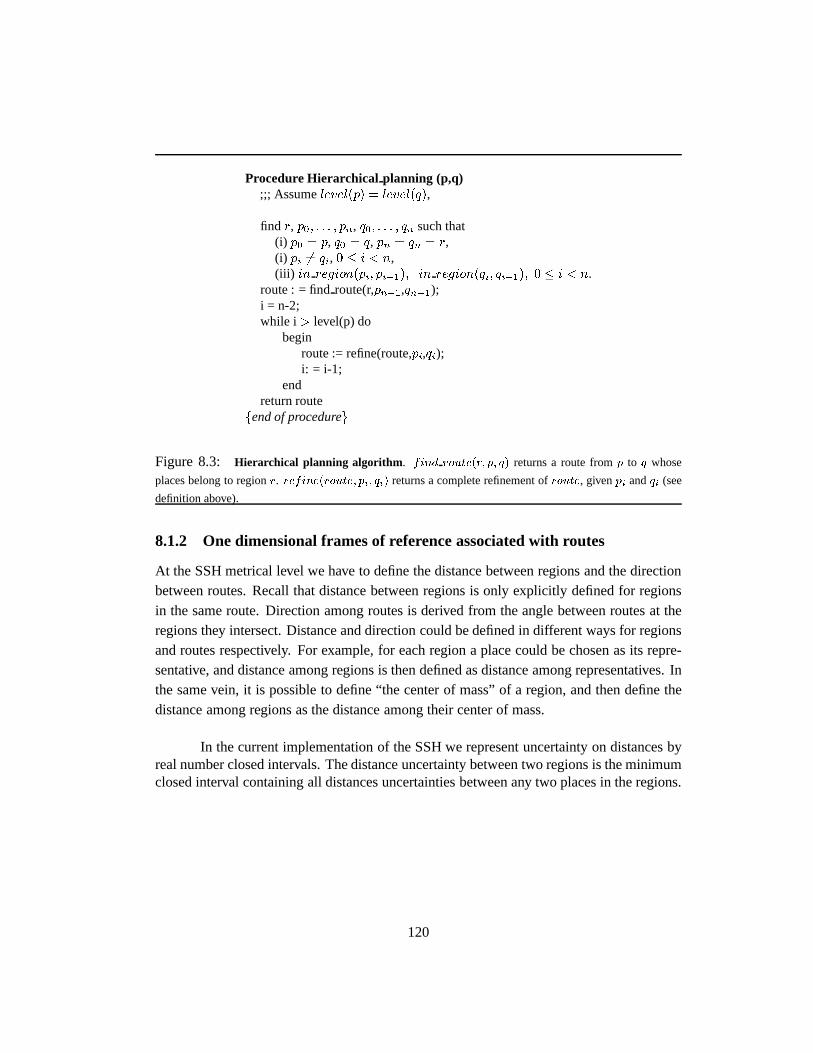
Procedure Hierarchical planning (p,q);;; Assumelevel(p) = level(q),

find r, p0; : : : ; pn, q0; : : : ; qn such that(i) p0 = p, q0 = q, pn = qn = r,(i) pi 6= qi, 0 � i < n,(iii) in region(pi; pi+1); in region(qi; qi+1); 0 � i < n.

route : = findroute(r,pn�1,qn�1);i = n-2;while i > level(p) do

beginroute := refine(route,pi,qi);i: = i-1;

endreturn route

fend of procedureg

Figure 8.3: Hierarchical planning algorithm . find route(r; p; q) returns a route fromp to q whose

places belong to regionr. refine(route; pi; qi) returns a complete refinement ofroute, givenpi andqi (see

definition above).

8.1.2 One dimensional frames of reference associated with routes

At the SSH metrical level we have to define the distance between regions and the directionbetween routes. Recall that distance between regions is only explicitly defined for regionsin the same route. Direction among routes is derived from the angle between routes at theregions they intersect. Distance and direction could be defined in different ways for regionsand routes respectively. For example, for each region a place could be chosen as its repre-sentative, and distance among regions is then defined as distance among representatives. Inthe same vein, it is possible to define “the center of mass” of a region, and then define thedistance among regions as the distance among their center of mass.

In the current implementation of the SSH we represent uncertainty on distances byreal number closed intervals. The distance uncertainty between two regions is the minimumclosed interval containing all distances uncertainties between any two places in the regions.

120

Formally,8 9

order(pa1; dir; r1; r2) ^ (8.6)

a = minfa0 : 9pa; p; q [lifted to(pa; pa1); in region(p; r1); in region(q; r2);

path distance�(pa; p; q; [a0; b0])]g ^

b = maxfb0 : 9pa; p; q [lifted to(pa; pa1); in region(p; r1); in region(q; r2);

path distance�(pa; p; q; [a0; b0])]g

! path distance�(pa1; r1; r2; [a; b])

8.1.3 Radial frames of reference associated with regions

In order to define the angle between paths at a region, we associate a two dimensional frameof reference with a region. Each place in the region gets a location with respect to this frameof reference (see section 7.2.3, page 96). We assume that the center of mass of the differentplace locations is(0; 0).10 The angle associated with the locations where a path enters orleaves a regions are used to assign the respective path headings with respect to the region:

A = fang : 9pa0; pa10; p; q; hp; hq

[lifted to(pa0; pa); lifted to(pa10; pa1);

place leaves(pa; dir; r; p); place leaves(pa10; dir1; r; q);

location2(r; p; lp); location2(r; q; lq)

directed angle(lp; lq) = a]

g ^

ang = min int cover(A)

! angle�(r; pa; dir; pa1; dir1; Iang)

wheremin int cover(A) denotes the minimum angle interval covering all the angles inthe setA. Example 30 (page 122) shows how all the above axioms work in aT like envi-ronment.

The resulting hierarchical representation is similar to the Hierarchical Graphs (AH-graphs) representation proposed in[Fernandez and Gonzalez, 1997, Fernandez and Gonza-lez, 1998, Fernandez, 2000]. They differ in that ours focuses on topological paths (not just

8Notation: Whenever a formula� is a conjunction,� = C1 ^ : : : ^Cn, we will replace by a comma andwriteC1; : : : ; Cn.

9The predicatepath distance�(pa; p; q; Id) is used to represent the fact that the closed intervalId is anestimate of the distance between placesp andq on pathpa. See page 93.

10Once a two dimensional frame of reference is created, the center of mass of the different places can becalculated, and places’ locations can be translated so that their center of mass become(0; 0).

121

edges in a graph), metrical information, and it is defined using an axiomatic theory compat-ible with the previous description of the SSH. In addition, we have not paid attention to theoptimality conditions the hierarchy should satisfy in order to find optimal navigation pathsat the bottom level of the hierarchy. Nevertheless, our specifications of regions has beenimplemented using AH-graphs[Remolinaet al., 1999].

8.2 Creating Regions

While we have described how to represent regions in the SSH, the question of how theagent learns such regions is not in the scope of this work. Nevertheless, we consider twogeneral approaches –metrical and topological– that lead to useful hierarchies in office-likeenvironments. In the metrical approach, places that are close to each other define a region.In the topological approach, objects or configurations of objects in the topological mapdefine regions. For instance, in chapter 6 boundary regions were defined by associatingwith a path its left and right regions. The basic algorithm to create a region hierarchy ispresented in figure 8.6 (page 125) . Although the algorithm only uses method (8.7) tocreate regions, any combination of methods could have been used.

Metrical approach

In this method, a regionr is a set of connected places such that if a placep is in r and thedistance fromp to placeq is less than a given threshold, then placeq is in r. Formally,

in region(p; r) ^ path distance(pa; p; q; d) ^ d � �! in region(q; r) (8.7)

The next example illustrates the use of this technique.

Example 30

Consider the environment in figure 8.4, where the agent has identified placesa throughh.Notice that placesb; c; e; f; g are very close one from each other. We can automatically set athreshold such that these places become a region,B. In virtue of axiom 8.7 (and the choiceof our threshold) placea gets associated to a regionA whose only place isa. Similarly,placesd andh get associated with regionsD = fdg andH = fhg, respectively. Note thatfor too large a threshold, or too uniform a distribution of places, all places will fall into thesame region, rendering the resulting region structure not useful.

Once these regions have been created, the pathha; b; e; c; di can be lifted to the pathhA;B;Di and the pathhb; f; g; hi can be lifted to the pathhB;Hi. The resulting topolog-ical map has two routes and four regions, as illustrated in figure 8.4b. Notice that the path

122

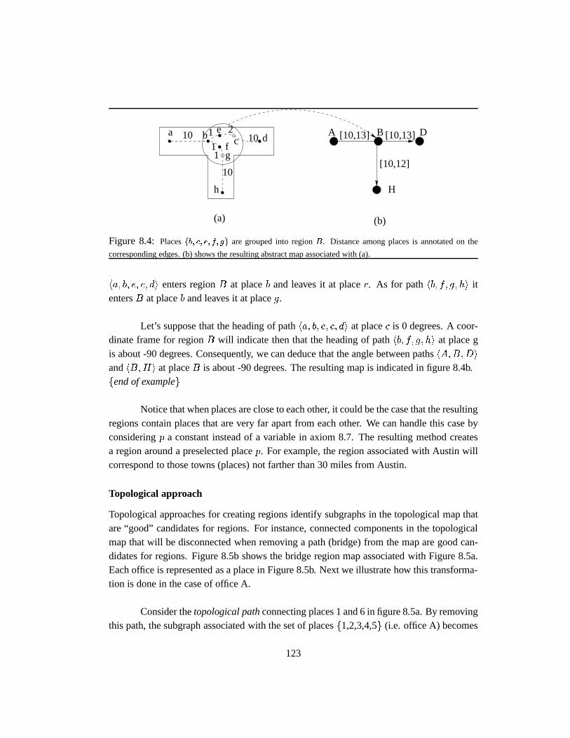
(a) (b)

H

[10,12]

[10,13] DBA10a

h

102e

fg

c

10

11

b1 d [10,13]

Figure 8.4: Placesfb; c; e; f; gg are grouped into regionB. Distance among places is annotated on the

corresponding edges. (b) shows the resulting abstract map associated with (a).

ha; b; e; c; di enters regionB at placeb and leaves it at placec. As for pathhb; f; g; hi itentersB at placeb and leaves it at placeg.

Let’s suppose that the heading of pathha; b; e; c; di at placec is 0 degrees. A coor-dinate frame for regionB will indicate then that the heading of pathhb; f; g; hi at place gis about -90 degrees. Consequently, we can deduce that the angle between pathshA;B;Di

andhB;Hi at placeB is about -90 degrees. The resulting map is indicated in figure 8.4b.fend of exampleg

Notice that when places are close to each other, it could be the case that the resultingregions contain places that are very far apart from each other. We can handle this case byconsideringp a constant instead of a variable in axiom 8.7. The resulting method createsa region around a preselected placep. For example, the region associated with Austin willcorrespond to those towns (places) not farther than 30 miles from Austin.

Topological approach

Topological approaches for creating regions identify subgraphs in the topological map thatare “good” candidates for regions. For instance, connected components in the topologicalmap that will be disconnected when removing a path (bridge) from the map are good can-didates for regions. Figure 8.5b shows the bridge region map associated with Figure 8.5a.Each office is represented as a place in Figure 8.5b. Next we illustrate how this transforma-tion is done in the case of office A.

Consider thetopological pathconnecting places 1 and 6 in figure 8.5a. By removingthis path, the subgraph associated with the set of placesf1,2,3,4,5g (i.e. office A) becomes

123

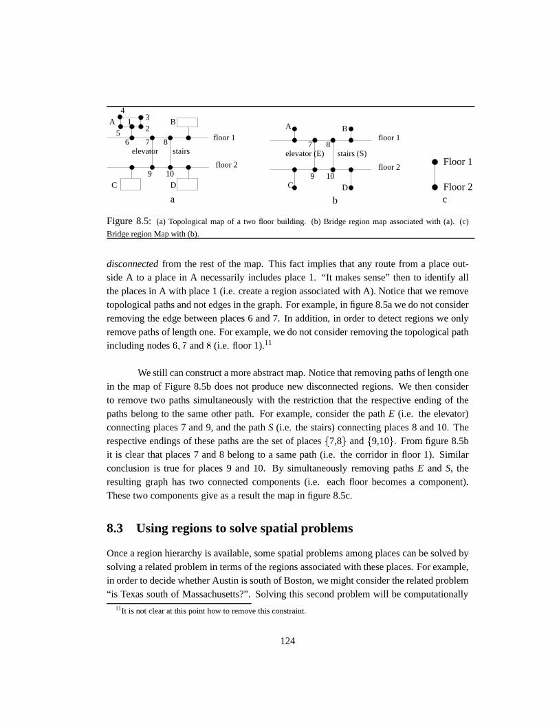
C

stairs

D

floor 2

1 B

76

A4

23

58 floor 1

9 10

elevator

C

elevator (E)7

BAfloor 1

floor 2

D9 10

8stairs (S)

Floor 2

Floor 1

a b c

Figure 8.5: (a) Topological map of a two floor building. (b) Bridge region map associated with (a). (c)

Bridge region Map with (b).

disconnectedfrom the rest of the map. This fact implies that any route from a place out-side A to a place in A necessarily includes place 1. “It makes sense” then to identify allthe places in A with place 1 (i.e. create a region associated with A). Notice that we removetopological paths and not edges in the graph. For example, in figure 8.5a we do not considerremoving the edge between places 6 and 7. In addition, in order to detect regions we onlyremove paths of length one. For example, we do not consider removing the topological pathincluding nodes6; 7 and8 (i.e. floor 1).11

We still can construct a more abstract map. Notice that removing paths of length onein the map of Figure 8.5b does not produce new disconnected regions. We then considerto remove two paths simultaneously with the restriction that the respective ending of thepaths belong to the same other path. For example, consider the pathE (i.e. the elevator)connecting places 7 and 9, and the pathS (i.e. the stairs) connecting places 8 and 10. Therespective endings of these paths are the set of placesf7,8g andf9,10g. From figure 8.5bit is clear that places 7 and 8 belong to a same path (i.e. the corridor in floor 1). Similarconclusion is true for places 9 and 10. By simultaneously removing pathsE and S, theresulting graph has two connected components (i.e. each floor becomes a component).These two components give as a result the map in figure 8.5c.

8.3 Using regions to solve spatial problems

Once a region hierarchy is available, some spatial problems among places can be solved bysolving a related problem in terms of the regions associated with these places. For example,in order to decide whether Austin is south of Boston, we might consider the related problem“is Texas south of Massachusetts?”. Solving this second problem will be computationally

11It is not clear at this point how to remove this constraint.

124

1. places := set of all places at the topological level.paths := { pa : on(pa,p), p in places}

2. do until |places| in {0,1}{

regions := emptysetnewpaths := emptyset

do until (places = emptyset) /* create regions */{

pick p in placescreate a new region r. Declare in_region(p,r)apply (8.7) until no more places can be grouped in rplaces := places \ {p: in_region(p,r)}regions := regions U {r}Create a frame of reference for r. Assign locations and headings

to places and paths in r.}

For pa in paths do /* lift paths */{

if pa has places in at least two different regionsthen

{create a new path pa’. Declare lifted(pa,pa’)apply lifting axiom (8.1) to path pa’.newpaths := newpaths U {pa’}

}}

places := regionspaths := newpaths

}

Figure 8.6:Basic algorithm to create region based topological maps.

125

less expensive than solving the original one, once the region hierarchy is created.

The key issue when working with a region hierarchy is to establish what proper-ties are preserved when moving up and down the hierarchy. These properties will allowus to establish the soundness of reasoning mechanisms based on regions as well as char-acterize the typical errors people might make when using regions to infer properties of theplaces in them. For instance, in the example above, we assumed that both problems, “isAustin south of Boston?” and “is Texas south of Massachusetts?”, are equivalent, that is,our region hierarchy preserves orientation information for places in the regionsTexas andMassachusetts. Notice that this is not necessarily always the case. For example, infor-mation of the relative orientation ofTexas andLouisiana does not help to decide whether“Austin is south of New Orleans”.12

8.4 Summary

In this chapter we extended the SSH topological level ontology to includeregions. Regionsare the basic abstraction mechanism the agent has in order to cope with the large numberof distinctive states (and so topological places) it will identify in the environment. Connec-tivity relations among regions were defined according to our lifting axiom 8.1, which stateshow to abstract the order of places in a path to the order of their corresponding regions ina route (our name for “abstract” paths). We then defined the distance among regions andthe angle among routes at their intersection places. In both cases, this metrical informationis derived from the metrical information among the places and paths being abstracted toregions and routes, respectively. In order to do so, we require a region to have a frame ofreference where places in the region are located.

The constraints imposed in the hierarchy of regions and paths do not exclude bizarrestructures. We defined a kind of hierarchies, stratified hierarchies, where it is guaranteedthat any route among regions has associated a sequence of actions at the SSH control level.We then presented an algorithm to do so.

Finally, we have defined different criteria for automatically creating regions. Whilethese methods are appropriate for office like environments, we have not addressed the prob-lem of what criteria should the agent use, when should it use them, and how does the agent

12[Stevens and Coupe, 1978] study illustrates how people incorrectly uses these hierarchies by making con-clusions like “San Diego is west of Reno NV” since “California is west of Nevada”.

126

obtains such criteria. Our approach has been completely pragmatic and the goal has beento devise criteria and algorithms for use in robotics.

127

Chapter 9

Implementation

The goal of this chapter is to illustrate the use of the theoretical ideas presented through thisdissertation, as well as to present some problems and techniques not covered by the theorybut required for its successful implementation (for instance, how to implement control laws,views, etc.).

Implementing the SSH control level requires one to define a set of control laws anda transformation from sensory input to views. Once this has been done, a set of schemas canbe generated by exploring the environment. This set of schemas constitutes the input for theother levels of the SSH. In this chapter we describe the SSH control level implementation,and describe the learned maps in two particular environments: a rectangular environment(Section 9.5.1) and Taylor Hall second floor (Section 9.5.2). The first environment illus-trates how boundary information is used to handle view aliasing. The second environmentillustrates the kind of map learned in a natural office-like environment. In addition, we de-fine an algorithm to track the different causal and topological maps associated with a set ofexperiences (if more than one map exists!).

The SSH’s implementation described in this chapter has been carried out in Vulcan,our wheelchair robot (Section 9.1). In section 9.2 we describe the control laws used inour experiments. How to define views is described in section 9.3. Section 9.4 presentsour implementation of the causal and topological levels. Finally, we present a trace of theexploration of the rectangular and Taylor Hall second floor environments in section 9.5.

128

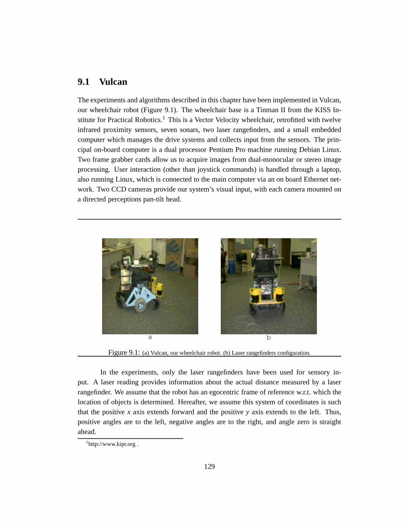
9.1 Vulcan

The experiments and algorithms described in this chapter have been implemented in Vulcan,our wheelchair robot (Figure 9.1). The wheelchair base is a Tinman II from the KISS In-stitute for Practical Robotics.1 This is a Vector Velocity wheelchair, retrofitted with twelveinfrared proximity sensors, seven sonars, two laser rangefinders, and a small embeddedcomputer which manages the drive systems and collects input from the sensors. The prin-cipal on-board computer is a dual processor Pentium Pro machine running Debian Linux.Two frame grabber cards allow us to acquire images from dual-monocular or stereo imageprocessing. User interaction (other than joystick commands) is handled through a laptop,also running Linux, which is connected to the main computer via an on board Ethernet net-work. Two CCD cameras provide our system’s visual input, with each camera mounted ona directed perceptions pan-tilt head.

a b

Figure 9.1:(a) Vulcan, our wheelchair robot. (b) Laser rangefinders configuration.

In the experiments, only the laser rangefinders have been used for sensory in-put. A laser reading provides information about the actual distance measured by a laserrangefinder. We assume that the robot has an egocentric frame of reference w.r.t. which thelocation of objects is determined. Hereafter, we assume this system of coordinates is suchthat the positivex axis extends forward and the positivey axis extends to the left. Thus,positive angles are to the left, negative angles are to the right, and angle zero is straightahead.

1http://www.kipr.org .

129

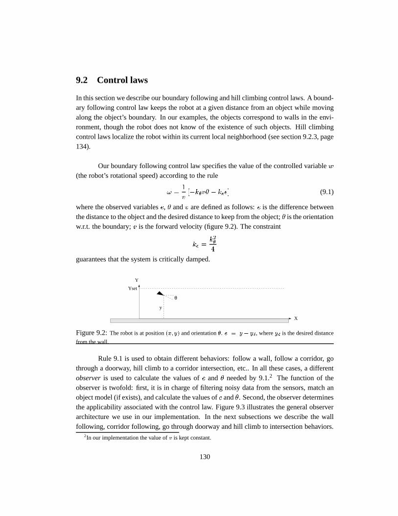
9.2 Control laws

In this section we describe our boundary following and hill climbing control laws. A bound-ary following control law keeps the robot at a given distance from an object while movingalong the object’s boundary. In our examples, the objects correspond to walls in the envi-ronment, though the robot does not know of the existence of such objects. Hill climbingcontrol laws localize the robot within its current local neighborhood (see section 9.2.3, page134).

Our boundary following control law specifies the value of the controlled variablew

(the robot’s rotational speed) according to the rule

! =1

v[�k�v� � kee] (9.1)

where the observed variablese, � andv are defined as follows:e is the difference betweenthe distance to the object and the desired distance to keep from the object;� is the orientationw.r.t. the boundary;v is the forward velocity (figure 9.2). The constraint

ke =k2�4

guarantees that the system is critically damped.

Yset

Y

X

y

θ

Figure 9.2:The robot is at position(x; y) and orientation�. e = y � yd, whereyd is the desired distance

from the wall.

Rule 9.1 is used to obtain different behaviors: follow a wall, follow a corridor, gothrough a doorway, hill climb to a corridor intersection, etc.. In all these cases, a differentobserveris used to calculate the values ofe and � needed by 9.1.2 The function of theobserver is twofold: first, it is in charge of filtering noisy data from the sensors, match anobject model (if exists), and calculate the values ofe and�. Second, the observer determinesthe applicability associated with the control law. Figure 9.3 illustrates the general observerarchitecture we use in our implementation. In the next subsections we describe the wallfollowing, corridor following, go through doorway and hill climb to intersection behaviors.

2In our implementation the value ofv is kept constant.

130

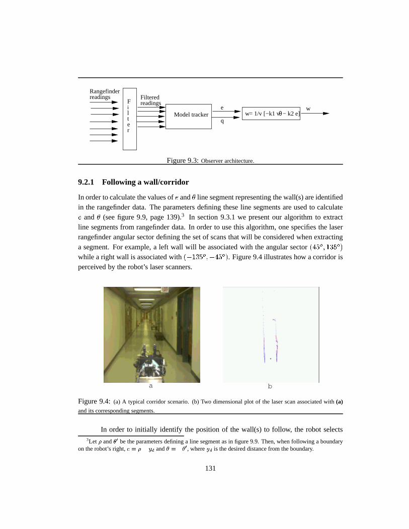
i

Rangefinderreadings

F

lter

Filteredreadings

Model trackere

qw

w= 1/v [−k1 v − k2 e]θ

Figure 9.3:Observer architecture.

9.2.1 Following a wall/corridor

In order to calculate the values ofe and� line segment representing the wall(s) are identifiedin the rangefinder data. The parameters defining these line segments are used to calculatee and� (see figure 9.9, page 139).3 In section 9.3.1 we present our algorithm to extractline segments from rangefinder data. In order to use this algorithm, one specifies the laserrangefinder angular sector defining the set of scans that will be considered when extractinga segment. For example, a left wall will be associated with the angular sector(45o; 135o)

while a right wall is associated with(�135o;�45o). Figure 9.4 illustrates how a corridor isperceived by the robot’s laser scanners.

a b

Figure 9.4:(a) A typical corridor scenario. (b) Two dimensional plot of the laser scan associated with(a)

and its corresponding segments.

In order to initially identify the position of the wall(s) to follow, the robot selects3Let � and�0 be the parameters defining a line segment as in figure 9.9. Then, when following a boundary

on the robot’s right,e = �� yd and� = ��0, whereyd is the desired distance from the boundary.

131

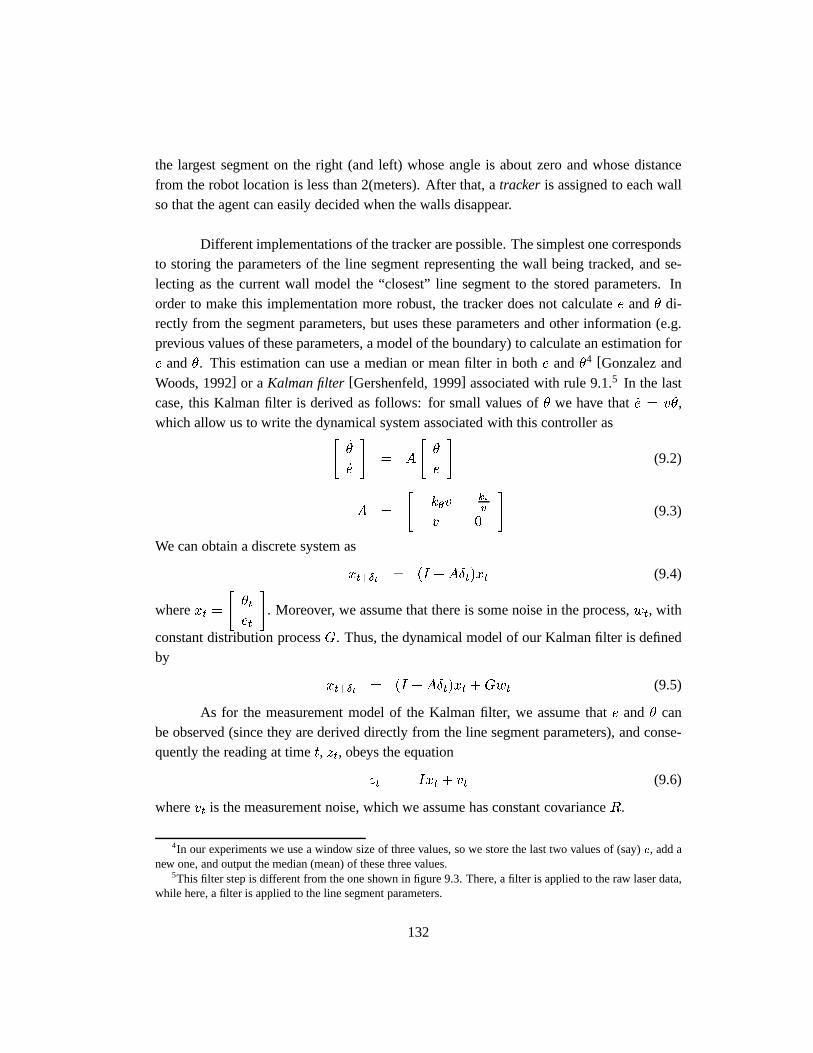
the largest segment on the right (and left) whose angle is about zero and whose distancefrom the robot location is less than 2(meters). After that, atracker is assigned to each wallso that the agent can easily decided when the walls disappear.

Different implementations of the tracker are possible. The simplest one correspondsto storing the parameters of the line segment representing the wall being tracked, and se-lecting as the current wall model the “closest” line segment to the stored parameters. Inorder to make this implementation more robust, the tracker does not calculatee and� di-rectly from the segment parameters, but uses these parameters and other information (e.g.previous values of these parameters, a model of the boundary) to calculate an estimation fore and�. This estimation can use a median or mean filter in bothe and�4 [Gonzalez andWoods, 1992] or aKalman filter[Gershenfeld, 1999] associated with rule 9.1.5 In the lastcase, this Kalman filter is derived as follows: for small values of� we have that_e = v�,which allow us to write the dynamical system associated with this controller as"

_�

_e

#= A

"�

e

#(9.2)

A =

"�k�v �ke

v

v 0

#(9.3)

We can obtain a discrete system as

xt+Æt = (I +AÆt)xt (9.4)

wherext =

"�tet

#. Moreover, we assume that there is some noise in the process,wt, with

constant distribution processG. Thus, the dynamical model of our Kalman filter is definedby

xt+Æt = (I +AÆt)xt +Gwt (9.5)

As for the measurement model of the Kalman filter, we assume thate and� canbe observed (since they are derived directly from the line segment parameters), and conse-quently the reading at timet, zt, obeys the equation

zt = Ixt + vt (9.6)

wherevt is the measurement noise, which we assume has constant covarianceR.

4In our experiments we use a window size of three values, so we store the last two values of (say)e, add anew one, and output the median (mean) of these three values.

5This filter step is different from the one shown in figure 9.3. There, a filter is applied to the raw laser data,while here, a filter is applied to the line segment parameters.

132

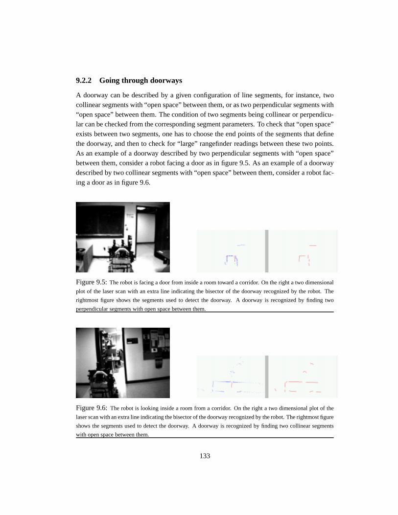
9.2.2 Going through doorways

A doorway can be described by a given configuration of line segments, for instance, twocollinear segments with “open space” between them, or as two perpendicular segments with“open space” between them. The condition of two segments being collinear or perpendicu-lar can be checked from the corresponding segment parameters. To check that “open space”exists between two segments, one has to choose the end points of the segments that definethe doorway, and then to check for “large” rangefinder readings between these two points.As an example of a doorway described by two perpendicular segments with “open space”between them, consider a robot facing a door as in figure 9.5. As an example of a doorwaydescribed by two collinear segments with “open space” between them, consider a robot fac-ing a door as in figure 9.6.

Figure 9.5:The robot is facing a door from inside a room toward a corridor. On the right a two dimensional

plot of the laser scan with an extra line indicating the bisector of the doorway recognized by the robot. The

rightmost figure shows the segments used to detect the doorway. A doorway is recognized by finding two

perpendicular segments with open space between them.

Figure 9.6:The robot is looking inside a room from a corridor. On the right a two dimensional plot of the

laser scan with an extra line indicating the bisector of the doorway recognized by the robot. The rightmost figure

shows the segments used to detect the doorway. A doorway is recognized by finding two collinear segments

with open space between them.

133

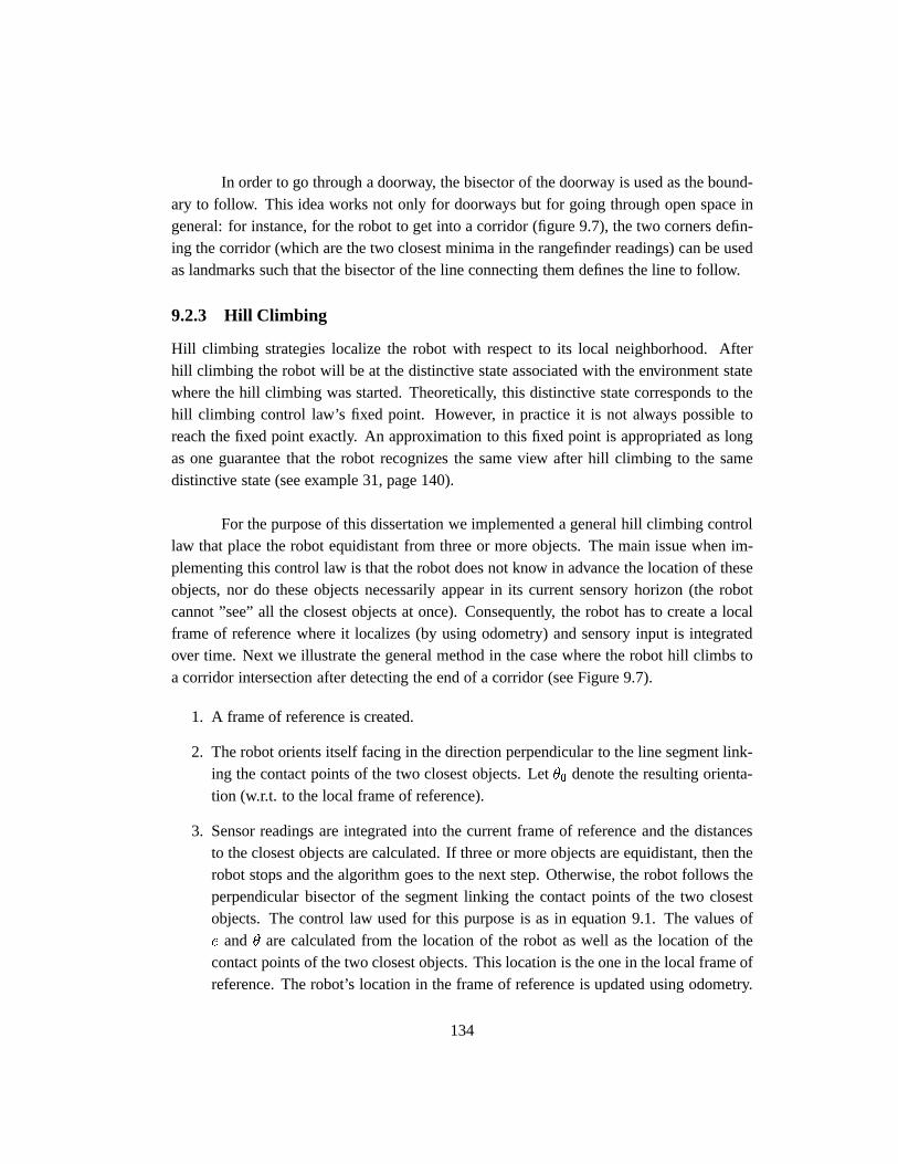
In order to go through a doorway, the bisector of the doorway is used as the bound-ary to follow. This idea works not only for doorways but for going through open space ingeneral: for instance, for the robot to get into a corridor (figure 9.7), the two corners defin-ing the corridor (which are the two closest minima in the rangefinder readings) can be usedas landmarks such that the bisector of the line connecting them defines the line to follow.

9.2.3 Hill Climbing

Hill climbing strategies localize the robot with respect to its local neighborhood. Afterhill climbing the robot will be at the distinctive state associated with the environment statewhere the hill climbing was started. Theoretically, this distinctive state corresponds to thehill climbing control law’s fixed point. However, in practice it is not always possible toreach the fixed point exactly. An approximation to this fixed point is appropriated as longas one guarantee that the robot recognizes the same view after hill climbing to the samedistinctive state (see example 31, page 140).

For the purpose of this dissertation we implemented a general hill climbing controllaw that place the robot equidistant from three or more objects. The main issue when im-plementing this control law is that the robot does not know in advance the location of theseobjects, nor do these objects necessarily appear in its current sensory horizon (the robotcannot ”see” all the closest objects at once). Consequently, the robot has to create a localframe of reference where it localizes (by using odometry) and sensory input is integratedover time. Next we illustrate the general method in the case where the robot hill climbs toa corridor intersection after detecting the end of a corridor (see Figure 9.7).

1. A frame of reference is created.

2. The robot orients itself facing in the direction perpendicular to the line segment link-ing the contact points of the two closest objects. Let�0 denote the resulting orienta-tion (w.r.t. to the local frame of reference).

3. Sensor readings are integrated into the current frame of reference and the distancesto the closest objects are calculated. If three or more objects are equidistant, then therobot stops and the algorithm goes to the next step. Otherwise, the robot follows theperpendicular bisector of the segment linking the contact points of the two closestobjects. The control law used for this purpose is as in equation 9.1. The values ofe and� are calculated from the location of the robot as well as the location of thecontact points of the two closest objects. This location is the one in the local frame ofreference. The robot’s location in the frame of reference is updated using odometry.

134

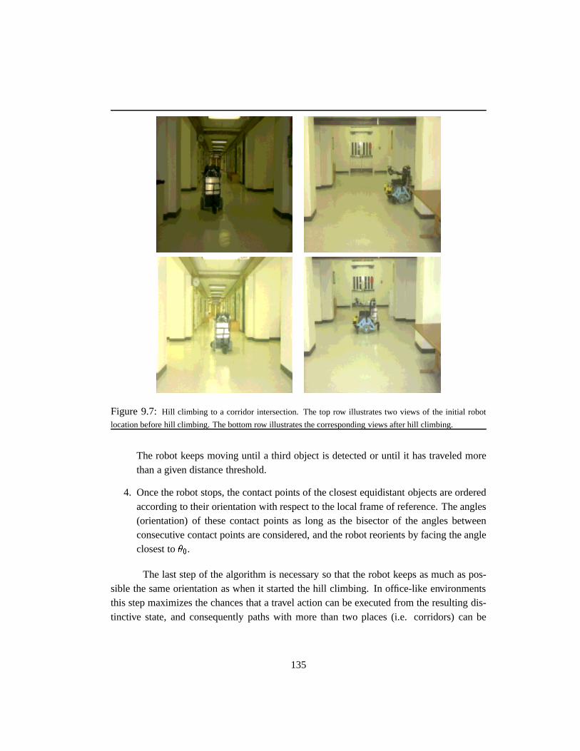
Figure 9.7:Hill climbing to a corridor intersection. The top row illustrates two views of the initial robot

location before hill climbing. The bottom row illustrates the corresponding views after hill climbing.

The robot keeps moving until a third object is detected or until it has traveled morethan a given distance threshold.

4. Once the robot stops, the contact points of the closest equidistant objects are orderedaccording to their orientation with respect to the local frame of reference. The angles(orientation) of these contact points as long as the bisector of the angles betweenconsecutive contact points are considered, and the robot reorients by facing the angleclosest to�0.

The last step of the algorithm is necessary so that the robot keeps as much as pos-sible the same orientation as when it started the hill climbing. In office-like environmentsthis step maximizes the chances that a travel action can be executed from the resulting dis-tinctive state, and consequently paths with more than two places (i.e. corridors) can be

135

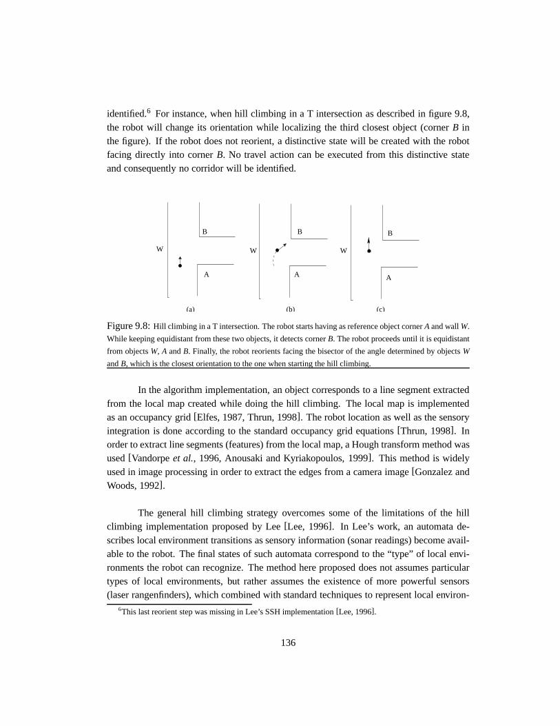
identified.6 For instance, when hill climbing in a T intersection as described in figure 9.8,the robot will change its orientation while localizing the third closest object (cornerB inthe figure). If the robot does not reorient, a distinctive state will be created with the robotfacing directly into cornerB. No travel action can be executed from this distinctive stateand consequently no corridor will be identified.

A

B

A A

BB

(b)(a) (c)

W W W

Figure 9.8:Hill climbing in a T intersection. The robot starts having as reference object cornerA and wallW.

While keeping equidistant from these two objects, it detects cornerB. The robot proceeds until it is equidistant

from objectsW, A andB. Finally, the robot reorients facing the bisector of the angle determined by objectsW

andB, which is the closest orientation to the one when starting the hill climbing.

In the algorithm implementation, an object corresponds to a line segment extractedfrom the local map created while doing the hill climbing. The local map is implementedas an occupancy grid[Elfes, 1987, Thrun, 1998]. The robot location as well as the sensoryintegration is done according to the standard occupancy grid equations[Thrun, 1998]. Inorder to extract line segments (features) from the local map, a Hough transform method wasused[Vandorpeet al., 1996, Anousaki and Kyriakopoulos, 1999]. This method is widelyused in image processing in order to extract the edges from a camera image[Gonzalez andWoods, 1992].

The general hill climbing strategy overcomes some of the limitations of the hillclimbing implementation proposed by Lee[Lee, 1996]. In Lee’s work, an automata de-scribes local environment transitions as sensory information (sonar readings) become avail-able to the robot. The final states of such automata correspond to the “type” of local envi-ronments the robot can recognize. The method here proposed does not assumes particulartypes of local environments, but rather assumes the existence of more powerful sensors(laser rangenfinders), which combined with standard techniques to represent local environ-

6This last reorient step was missing in Lee’s SSH implementation[Lee, 1996].

136

ments allow the robot to keep track of objects not visible in the current sensory image.

137

9.3 Views

Each distinctive state has associated a view symbol representing what the distinctive state“looks like”. In order to create such view the agent examines the sensory input associatedwith the distinctive state neighborhood. Views are created by considering the set of seg-ments associated with the rangefinder scan at the agent environment location.7 Next wedescribe our implementation and provide some experimental results (see example 31, page140) showing the appropriateness of the method.8

Each laser scan has associated a sequence of line segments(ls1; : : : ; lsn) whichconstitutes its view representation. This sequence of segments is found by extracting the setof line segments associated with the scan (see Section 9.3.1), and ordering them accordingto their angle.

The problem of finding how similar two scans are is reduced to the one of findinghow similar two finite sequences of line segments are. Anembeddingfrom (ls11; : : : ; ls1n)

into (ls21; : : : ; ls2m) is an increasingfunction from a set inchoose(min(n;m); n)9 intof1; : : : ;mg. The goodness of an embeddinge is defined as follows:

Goodness(e) =1

n

min(n;m)Xi=1

sim(ls1i; ls2e(i)) (9.7)

wheresim(l1; l2) is a positive function returning a value in[0; 1] indicating how similarline segmentsl1 andl2 are. We will provide a definition forsim later.

The similarity ofs1 = (ls11; : : : ; ls1n) w.r.t. s2 = (ls21; : : : ; ls2m) is given by

Sim(s1; s2) = maxe

Goodness(e) ;

the value of the best embedding ofs1 into s2. Finally, the match betweens1 ands2 is givenby

match(s1; s2) = min(Sim(s1; s2); Sim(s2; s1)) :

In order to calculatematch(s1; s2) an adaptation of thelongest common subse-quencesalgorithm can be done[Cormenet al., 1993]. Next we define how to compare line

7Different methods can be considered to create such view: create an occupancy grid of the dstate neigh-borhood, train a neural net, etc.. See[Duckett and Nehmzow, 2000] for a comparative study of these differentmethods.

8The work in this section is joint effort with Micheal Hewett.9Choose(k,n) denotes the subsets off1; : : : ; ng that havek elements.

138

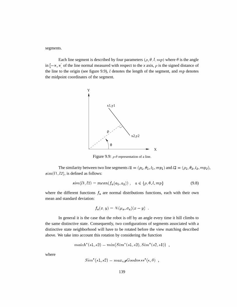
segments.

Each line segment is described by four parameters(�; �; l;mp) where� is the anglein [��; �] of the line normal measured with respect to thex axis,� is the signed distance ofthe line to the origin (see figure 9.9),l denotes the length of the segment, andmp denotesthe midpoint coordinates of the segment.

Y

X

x1,y1

x2,y2

θ

ρ

Figure 9.9:�-� representation of a line.

The similarity between two line segmentsl1 = (�1; �1; l1;mp1) andl2 = (�2; �2; l2;mp2),sim(l1; l2), is defined as follows:

sim(l1; l2) = mean(fa(a1; a2)) ; a 2 f�; �; l;mpg (9.8)

where the different functionsfa are normal distributions functions, each with their ownmean and standard deviation:

fa(x; y) = N(�a; �a)(x� y) :

In general it is the case that the robot is off by an angle every time it hill climbs tothe same distinctive state. Consequently, two configurations of segments associated with adistinctive state neighborhood will have to be rotated before the view matching describedabove. We take into account this rotation by considering the function

match�(s1; s2) = min(Sim�(s1; s2); Sim�(s2; s1)) ;

whereSim�(s1; s2) = maxe;�Goodness

�(e; �) ;

139

Goodness�(e; �) =1

n

min(n;m)Xi=1

sim(ls1�i ; ls2e(i)) ;

and l� denotes the line segment resulting of rotatingl by an angle�. The next exampleillustrates the appropriateness of the view matching defined in this section.

Example 31

Figure 9.10 illustrates different segment configurations associated with the distinctive stateresulting of hill climbing to a corridor intersection (see figure 9.7, page 135). Table 9.11shows the similarity values for these different configurations.

The values in table 9.11 represent the intraclass similarity corresponding to the view(class) associated with the distinctive state. In this table, scan 3 is taken at the ideal distinc-tive state location: the wheelchair perfectly aligns with the corridors (see figure 9.7, page135). Notice how the similarity values decrease as the orientation changes with respect toscan 3. For instance, scans 1 and 5 differ by about10Æ and their similarity value is only0:58.

While not shown, we have found that for most of our experiment0:6 is an appropri-ate threshold for deciding whether two segment configurations correspond to the same view(class). As illustrated in section 9.5.2 (page 176), this threshold is way above the similarityvalues obtained for scans taken at different distinctive states (i.e. extra-class similarities).While it is an interesting problem to formulate how the agent learns this threshold, or forthat matter, how it decides how many classes (views) should be associated with its sensoryinput at distinctive states, that learning task is out the scope of this work.fend of exampleg

140

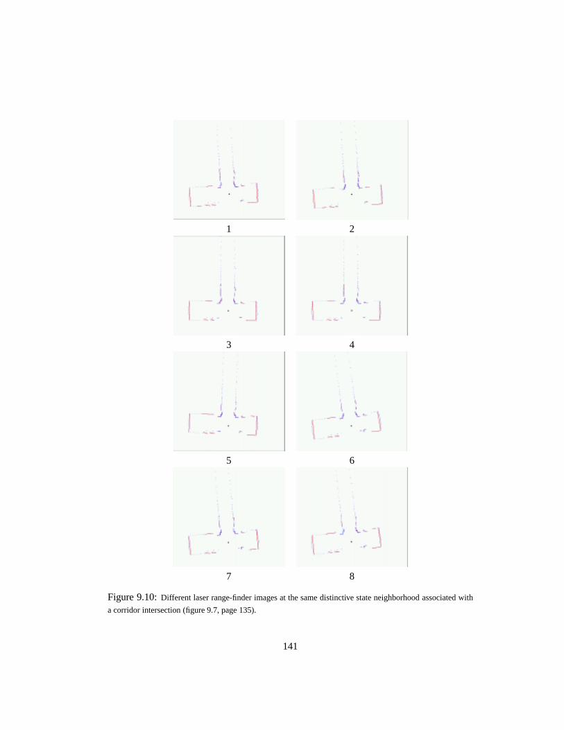
1 2

3 4

5 6

7 8

Figure 9.10:Different laser range-finder images at the same distinctive state neighborhood associated with

a corridor intersection (figure 9.7, page 135).

141

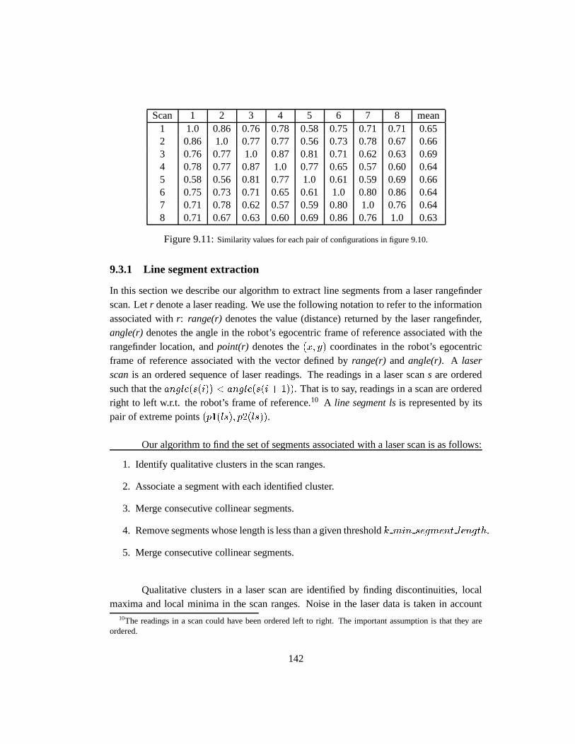
Scan 1 2 3 4 5 6 7 8 mean1 1.0 0.86 0.76 0.78 0.58 0.75 0.71 0.71 0.652 0.86 1.0 0.77 0.77 0.56 0.73 0.78 0.67 0.663 0.76 0.77 1.0 0.87 0.81 0.71 0.62 0.63 0.694 0.78 0.77 0.87 1.0 0.77 0.65 0.57 0.60 0.645 0.58 0.56 0.81 0.77 1.0 0.61 0.59 0.69 0.666 0.75 0.73 0.71 0.65 0.61 1.0 0.80 0.86 0.647 0.71 0.78 0.62 0.57 0.59 0.80 1.0 0.76 0.648 0.71 0.67 0.63 0.60 0.69 0.86 0.76 1.0 0.63

Figure 9.11:Similarity values for each pair of configurations in figure 9.10.

9.3.1 Line segment extraction

In this section we describe our algorithm to extract line segments from a laser rangefinderscan. Letr denote a laser reading. We use the following notation to refer to the informationassociated withr: range(r) denotes the value (distance) returned by the laser rangefinder,angle(r)denotes the angle in the robot’s egocentric frame of reference associated with therangefinder location, andpoint(r) denotes the(x; y) coordinates in the robot’s egocentricframe of reference associated with the vector defined byrange(r) andangle(r). A laserscanis an ordered sequence of laser readings. The readings in a laser scans are orderedsuch that theangle(s(i)) < angle(s(i+ 1)). That is to say, readings in a scan are orderedright to left w.r.t. the robot’s frame of reference.10 A line segment lsis represented by itspair of extreme points(p1(ls); p2(ls)).

Our algorithm to find the set of segments associated with a laser scan is as follows:

1. Identify qualitative clusters in the scan ranges.

2. Associate a segment with each identified cluster.

3. Merge consecutive collinear segments.

4. Remove segments whose length is less than a given thresholdk min segment length.

5. Merge consecutive collinear segments.

Qualitative clusters in a laser scan are identified by finding discontinuities, localmaxima and local minima in the scan ranges. Noise in the laser data is taken in account

10The readings in a scan could have been ordered left to right. The important assumption is that they areordered.

142

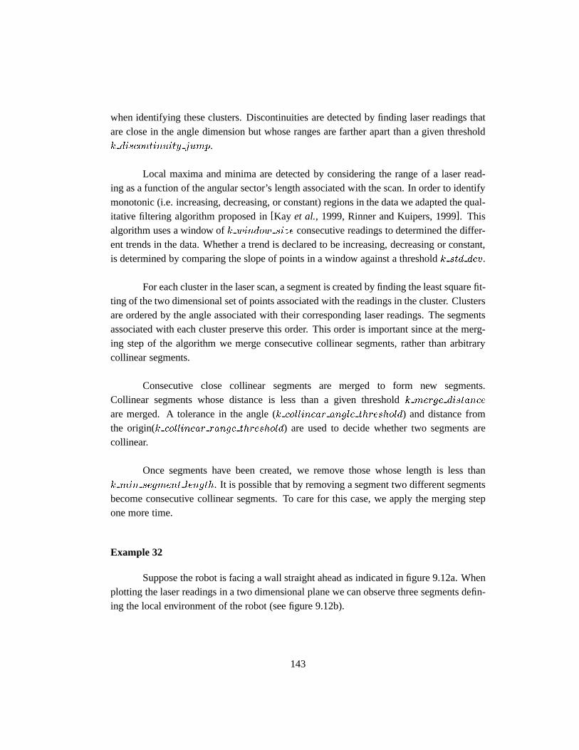
when identifying these clusters. Discontinuities are detected by finding laser readings thatare close in the angle dimension but whose ranges are farther apart than a given thresholdk discontinuity jump.

Local maxima and minima are detected by considering the range of a laser read-ing as a function of the angular sector’s length associated with the scan. In order to identifymonotonic (i.e. increasing, decreasing, or constant) regions in the data we adapted the qual-itative filtering algorithm proposed in[Kay et al., 1999, Rinner and Kuipers, 1999]. Thisalgorithm uses a window ofk window size consecutive readings to determined the differ-ent trends in the data. Whether a trend is declared to be increasing, decreasing or constant,is determined by comparing the slope of points in a window against a thresholdk std dev.

For each cluster in the laser scan, a segment is created by finding the least square fit-ting of the two dimensional set of points associated with the readings in the cluster. Clustersare ordered by the angle associated with their corresponding laser readings. The segmentsassociated with each cluster preserve this order. This order is important since at the merg-ing step of the algorithm we merge consecutive collinear segments, rather than arbitrarycollinear segments.

Consecutive close collinear segments are merged to form new segments.Collinear segments whose distance is less than a given thresholdk merge distance

are merged. A tolerance in the angle (k collinear angle threshold) and distance fromthe origin(k collinear range threshold) are used to decide whether two segments arecollinear.

Once segments have been created, we remove those whose length is less thank min segment length. It is possible that by removing a segment two different segmentsbecome consecutive collinear segments. To care for this case, we apply the merging stepone more time.

Example 32

Suppose the robot is facing a wall straight ahead as indicated in figure 9.12a. Whenplotting the laser readings in a two dimensional plane we can observe three segments defin-ing the local environment of the robot (see figure 9.12b).

143

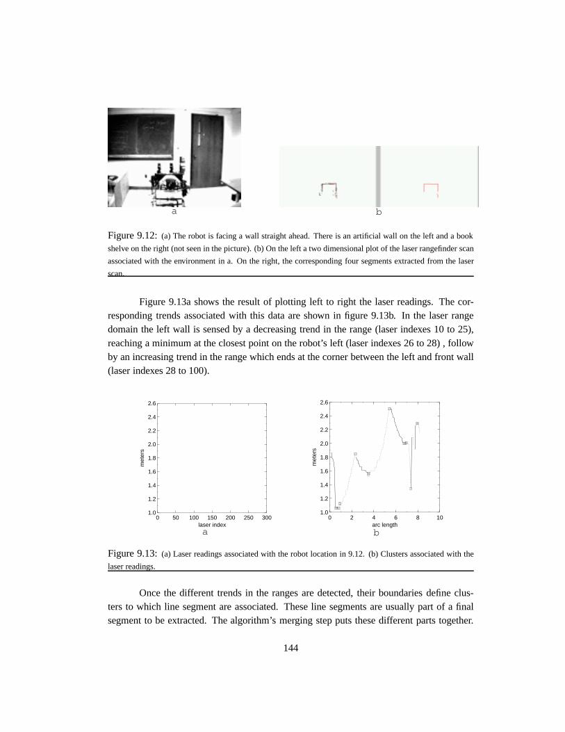
a b

Figure 9.12:(a) The robot is facing a wall straight ahead. There is an artificial wall on the left and a book

shelve on the right (not seen in the picture). (b) On the left a two dimensional plot of the laser rangefinder scan

associated with the environment in a. On the right, the corresponding four segments extracted from the laser

scan.

Figure 9.13a shows the result of plotting left to right the laser readings. The cor-responding trends associated with this data are shown in figure 9.13b. In the laser rangedomain the left wall is sensed by a decreasing trend in the range (laser indexes 10 to 25),reaching a minimum at the closest point on the robot’s left (laser indexes 26 to 28) , followby an increasing trend in the range which ends at the corner between the left and front wall(laser indexes 28 to 100).

0 50 100 150 200 250 3001.0

1.2

1.4

1.6

1.8

2.0

2.2

2.4

2.6

laser index

met

ers

0 2 4 6 8 101.0

1.2

1.4

1.6

1.8

2.0

2.2

2.4

2.6

arc length

met

ers

a b

Figure 9.13:(a) Laser readings associated with the robot location in 9.12. (b) Clusters associated with the

laser readings.

Once the different trends in the ranges are detected, their boundaries define clus-ters to which line segment are associated. These line segments are usually part of a finalsegment to be extracted. The algorithm’s merging step puts these different parts together.

144

For example, the left wall in figure 9.12 has associated three clusters indicated by the laserindexes 10, 25, 28 and 100. The resulting segments associated with these clusters are allcollinear, and consequently merged into one segment.fend of exampleg

Example 33

In order to identify qualitative clusters in the scan ranges, first we detect discon-tinuities (jumps) in the data. These discontinuities define clusters of readings on whichdecreasing, increasingor constanttrends are detected. These trends are the only patternsin the data used to define segments. While example 32 may suggest that it is possible toassociate a segment with more complex patterns in the data (e.g. “U” patterns), this is notnecessarily the case. For instance consider the case in which the robot has partial accessto different rooms (figure 9.14a). Figure 9.14b shows the laser rangefinder data and thesegments found by the algorithm.

As shown in figure 9.15a, the laser ranges have discontinuities and some walls arenot perceive in a “U” pattern as in example 32. However, the different up, down, and con-stant trends in the data do define part of the segments to be extracted. Whether two trendsare part of a same line segment is decided by assigning line segments to each trend and thenchecking for these segments to be collinear.fend of exampleg

145

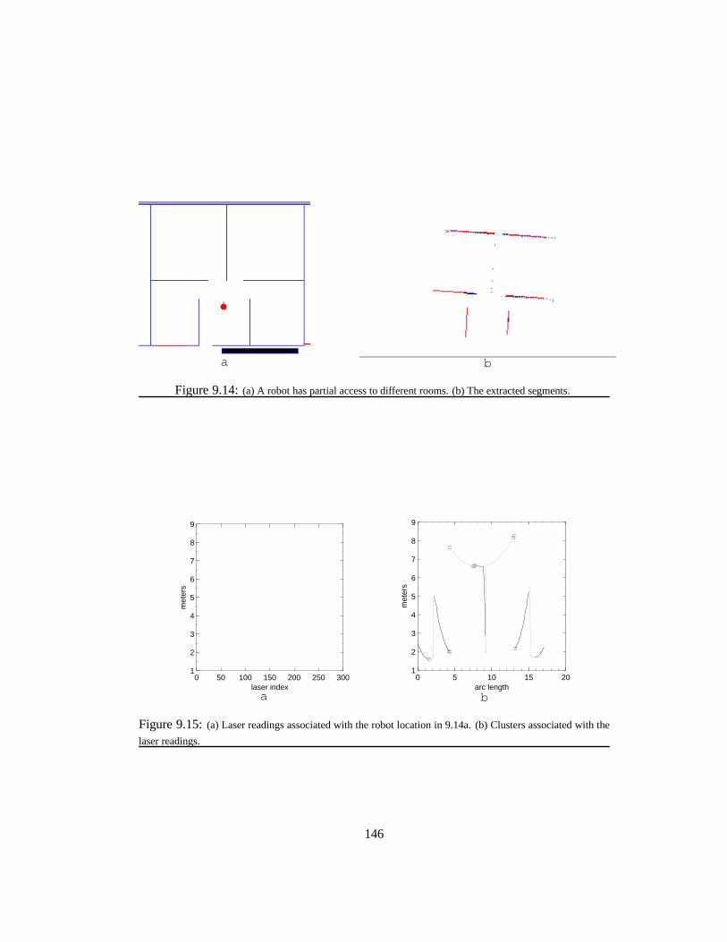
a b

Figure 9.14:(a) A robot has partial access to different rooms. (b) The extracted segments.

0 50 100 150 200 250 3001

2

3

4

5

6

7

8

9

laser index

met

ers

0 5 10 15 201

2

3

4

5

6

7

8

9

arc length

met

ers

a b

Figure 9.15:(a) Laser readings associated with the robot location in 9.14a. (b) Clusters associated with the

laser readings.

146

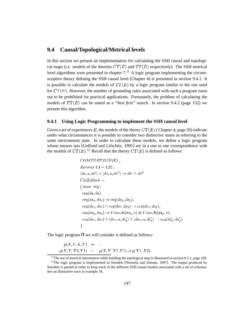
9.4 Causal/Topological/Metrical levels

In this section we present an implementation for calculating the SSH causal and topologi-cal maps (i.e. models of the theoriesCT (E) andTT (E) respectively). The SSH metricallevel algorithms were presented in chapter 7.11 A logic program implementing the circum-scriptive theory defining the SSH causal level (Chapter 4) is presented in section 9.4.1. Itis possible to calculate the models ofTT (E) by a logic program similar to the one usedfor CT (E). However, the number of grounding rules associated with such a program turnsout to be prohibited for practical applications. Fortunately, the problem of calculating themodels ofTT (E) can be stated as a“best first” search. In section 9.4.2 (page 152) wepresent this algorithm.

9.4.1 Using Logic Programming to implement the SSH causal level

Given a set of experiencesE, the models of the theoryCT (E) ( Chapter 4, page 26) indicateunder what circumstances it is possible to consider two distinctive states as referring to thesame environment state. In order to calculate these models, we define a logic programwhose answer sets[Gelfond and Lifschitz, 1991] are in a one to one correspondence withthe models ofCT (E).12 Recall that the theoryCT (E) is defined as follows:

COMPLETION(E) ;

Axioms 4:1� 4:22 ;

hds; a; ds0i ^ hds; a; ds00i ! ds0 = ds00

CEQ block =

f max ceq :

ceq(ds; ds);

ceq(ds1; ds2)! ceq(ds2; ds1);

ceq(ds1; ds2) ^ ceq(ds2; ds3)! ceq(ds1; ds3);

ceq(ds1; ds2)! V iewAt(ds1; v) � V iewAt(ds2; v);

ceq(ds1; ds2) ^ hds1; a; ds0

1i ^ hds2; a; ds0

2i ! ceq(ds01; ds0

2)

g

The logic program� we will consider is defined as follows:

p(X;Y;X; Y ) :

p(X;Y;X2; Y 1) p(X;Y;X1; Y 1); ceq(X1; X2):

11The use of metrical information while building the topological map is illustrated in section 9.5.1, page 169.12The logic program is implemented in Smodels[Niemel�a and Simons, 1997]. The output produced by

Smodels is parsed in order to keep track of the different SSH causal models associated with a set of schemas.See an illustrative trace in example 34.

147

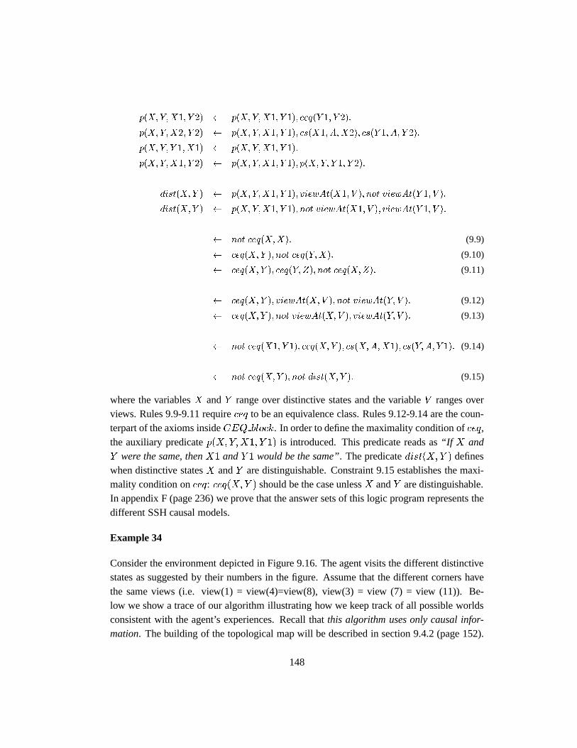
p(X;Y;X1; Y 2) p(X;Y;X1; Y 1); ceq(Y 1; Y 2):

p(X;Y;X2; Y 2) p(X;Y;X1; Y 1); cs(X1; A;X2); cs(Y 1; A; Y 2):

p(X;Y; Y 1; X1) p(X;Y;X1; Y 1):

p(X;Y;X1; Y 2) p(X;Y;X1; Y 1); p(X;Y; Y 1; Y 2):

dist(X;Y ) p(X;Y;X1; Y 1); viewAt(X1; V ); not viewAt(Y 1; V ):

dist(X;Y ) p(X;Y;X1; Y 1); not viewAt(X1; V ); viewAt(Y 1; V ):

not ceq(X;X): (9.9)

ceq(X;Y ); not ceq(Y;X): (9.10)

ceq(X;Y ); ceq(Y; Z); not ceq(X;Z): (9.11)

ceq(X;Y ); viewAt(X;V ); not viewAt(Y; V ): (9.12)

ceq(X;Y ); not viewAt(X;V ); viewAt(Y; V ): (9.13)

not ceq(X1; Y 1); ceq(X;Y ); cs(X;A;X1); cs(Y;A; Y 1): (9.14)

not ceq(X;Y ); not dist(X;Y ): (9.15)

where the variablesX andY range over distinctive states and the variableV ranges overviews. Rules 9.9-9.11 requireceq to be an equivalence class. Rules 9.12-9.14 are the coun-terpart of the axioms insideCEQ block. In order to define the maximality condition ofceq,the auxiliary predicatep(X;Y;X1; Y 1) is introduced. This predicate reads as“If X andY were the same, thenX1 andY 1 would be the same”. The predicatedist(X;Y ) defineswhen distinctive statesX andY are distinguishable. Constraint 9.15 establishes the maxi-mality condition onceq: ceq(X;Y ) should be the case unlessX andY are distinguishable.In appendix F (page 236) we prove that the answer sets of this logic program represents thedifferent SSH causal models.

Example 34

Consider the environment depicted in Figure 9.16. The agent visits the different distinctivestates as suggested by their numbers in the figure. Assume that the different corners havethe same views (i.e. view(1) = view(4)=view(8), view(3) = view (7) = view (11)). Be-low we show a trace of our algorithm illustrating how we keep track of all possible worldsconsistent with the agent’s experiences. Recall thatthis algorithm uses only causal infor-mation. The building of the topological map will be described in section 9.4.2 (page 152).

148

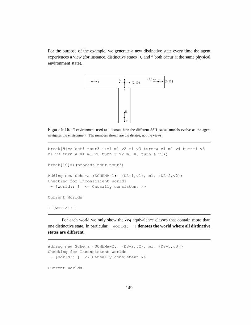
For the purpose of the example, we generate a new distinctive state every time the agentexperiences a view (for instance, distinctive states10 and2 both occur at the same physicalenvironment state).

����

��������

��������

����15

6

8

7

9

{2,10} {3,11}{4,12}

Figure 9.16: T-environment used to illustrate how the different SSH causal models evolve as the agent

navigates the environment. The numbers shown are the dstates, not the views.

break[9]=>(set! tour3 ’(v1 ml v2 ml v3 turn-a v1 ml v4 turn-l v5ml v3 turn-a v1 ml v6 turn-r v2 ml v3 turn-a v1))

break[10]=>(process-tour tour3)

Adding new Schema <SCHEMA-1:: (DS-1,v1), ml, (DS-2,v2)>Checking for Inconsistent worlds

- [world:: ] << Causally consistent >>

Current Worlds

1 [world:: ]

For each world we only show theceq equivalence classes that contain more thanone distinctive state. In particular,[world:: ] denotes the world where all distinctivestates are different.

Adding new Schema <SCHEMA-2:: (DS-2,v2), ml, (DS-3,v3)>Checking for Inconsistent worlds

- [world:: ] << Causally consistent >>

Current Worlds

149

1 [world:: ]

Adding new Schema <SCHEMA-3:: (DS-3,v3), turn-a, (DS-4,v1)>Checking for Inconsistent worlds

- [world:: ] << Causally consistent >>

Current Worlds

1. [world:: (DS-4 DS-1)]

At this point the agent cannot distinguishDS-1 from DS-4 , and so the agent hasonly one model of the world where these two distinctive states are the same.

Adding new Schema <SCHEMA-4:: (DS-4,v1), ml, (DS-5,v4)>

Checking for Inconsistent worlds

- [world:: (DS-4 DS-1)] << Causally Inconsistent >>>> Not Eq relations learned >>> {not-eq:{DS-1:: (DS-4)} {DS-4:: (DS-1)}}

Current Worlds

1 [world:: ]

Once the agent travels fromDS-4 to DS-5 and observes viewV 4, distinctive statesDS-1 andDS-4 become distinguishable, since executingml starting atDS-1 takes theagent to a distinctive state with viewV 2 which is different fromV 4. In addition, the agentlearns that in any possible world,DS-1neqDS-4 .

Adding new Schema <SCHEMA-5:: (DS-5,v4), turn-l, (DS-6,v5)>

Checking for Inconsistent worlds

- [world:: ] << Causally consistent >>

Current Worlds

1 [world:: ]

Adding new Schema <SCHEMA-6:: (DS-6,v5), ml, (DS-7,v3)>

Checking for Inconsistent worlds- [world:: ] << Causally consistent >>

Current Worlds

150

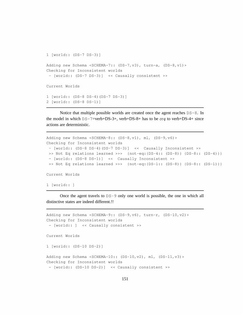
1 [world:: (DS-7 DS-3)]

Adding new Schema <SCHEMA-7:: (DS-7,v3), turn-a, (DS-8,v1)>

Checking for Inconsistent worlds- [world:: (DS-7 DS-3)] << Causally consistent >>

Current Worlds

1 [world:: (DS-8 DS-4)(DS-7 DS-3)]2 [world:: (DS-8 DS-1)]

Notice that multiple possible worlds are created once the agent reachesDS-8 . Inthe model in whichDS-7=verb+DS-3+, verb+DS-8+ has to beceq to verb+DS-4+ sinceactions are deterministic.

Adding new Schema <SCHEMA-8:: (DS-8,v1), ml, (DS-9,v6)>Checking for Inconsistent worlds

- [world:: (DS-8 DS-4)(DS-7 DS-3)] << Causally Inconsistent >>>> Not Eq relations learned >>> {not-eq:{DS-4:: (DS-8)} {DS-8:: (DS-4)}}

- [world:: (DS-8 DS-1)] << Causally Inconsistent >>

>> Not Eq relations learned >>> {not-eq:{DS-1:: (DS-8)} {DS-8:: (DS-1)}}

Current Worlds

1 [world:: ]

Once the agent travels toDS-9 only one world is possible, the one in which alldistinctive states are indeed different.!!

Adding new Schema <SCHEMA-9:: (DS-9,v6), turn-r, (DS-10,v2)>

Checking for Inconsistent worlds- [world:: ] << Causally consistent >>

Current Worlds

1 [world:: (DS-10 DS-2)]

Adding new Schema <SCHEMA-10:: (DS-10,v2), ml, (DS-11,v3)>Checking for Inconsistent worlds

- [world:: (DS-10 DS-2)] << Causally consistent >>

151

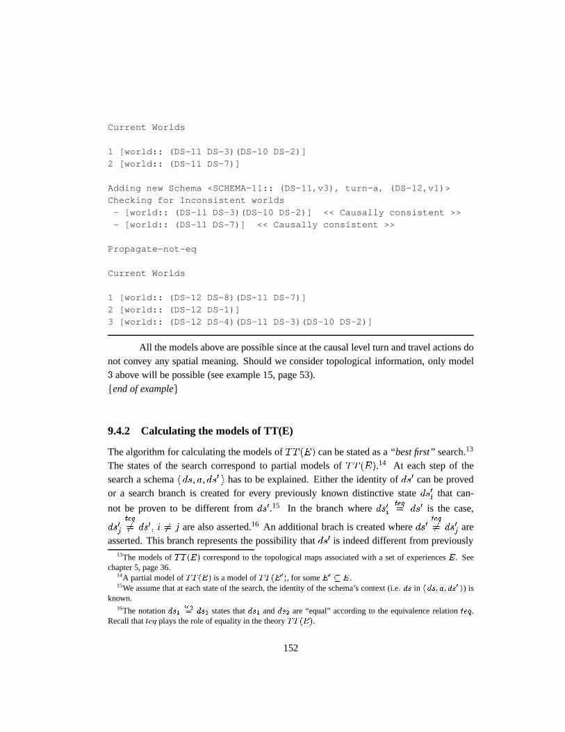
Current Worlds

1 [world:: (DS-11 DS-3)(DS-10 DS-2)]

2 [world:: (DS-11 DS-7)]

Adding new Schema <SCHEMA-11:: (DS-11,v3), turn-a, (DS-12,v1)>Checking for Inconsistent worlds

- [world:: (DS-11 DS-3)(DS-10 DS-2)] << Causally consistent >>

- [world:: (DS-11 DS-7)] << Causally consistent >>

Propagate-not-eq

Current Worlds

1 [world:: (DS-12 DS-8)(DS-11 DS-7)]

2 [world:: (DS-12 DS-1)]3 [world:: (DS-12 DS-4)(DS-11 DS-3)(DS-10 DS-2)]

All the models above are possible since at the causal level turn and travel actions donot convey any spatial meaning. Should we consider topological information, only model3 above will be possible (see example 15, page 53).fend of exampleg

9.4.2 Calculating the models of TT(E)

The algorithm for calculating the models ofTT (E) can be stated as a“best first” search.13

The states of the search correspond to partial models ofTT (E).14 At each step of thesearch a schemah ds; a; ds0 i has to be explained. Either the identity ofds0 can be provedor a search branch is created for every previously known distinctive stateds0i that can-

not be proven to be different fromds0.15 In the branch whereds0iteq= ds0 is the case,

ds0jteq

6= ds0; i 6= j are also asserted.16 An additional brach is created whereds0teq

6= ds0j areasserted. This branch represents the possibility thatds0 is indeed different from previously

13The models ofTT (E) correspond to the topological maps associated with a set of experiencesE. Seechapter 5, page 36.

14A partial model ofTT (E) is a model ofTT (E0), for someE0 � E.15We assume that at each state of the search, the identity of the schema’s context (i.e.ds in hds; a; ds0 i) is

known.16The notationds1

teq= ds2 states thatds1 andds2 are “equal” according to the equivalence relationteq.

Recall thatteq plays the role of equality in the theoryTT (E).

152

known dstates. The next state to explore is the one that is minimal according to the orderassociated with the circumscription policy forTT (E). This search algorithm is describedin figures 9.17 and 9.18.17

Find-Models (Schemas S)f

;; S =s0; : : : ; sn ; sequence of schemas such that;; result(si) = context(si+1);;;; pmodels-to-explore = ordered queue of partial models to explore.;; models = list of total models for S.pmodels-to-explore =; ;models =; ;pmodel = create-new-pmodel(S);insert(pmodel,pmodels-to-explore) ;while pmodels-to-explore6= ; dobeginpmodel = get-next-pmodel(pmodels-to-explore);s = get-next-schema(pmodel);Explain(pmodel,s) ;if (inconsistent(pmodel)_ has-extensions(pmodel)) then skip;else if total-model(pmodel) then insert(pmodel, models);else insert(pmodel,pmodels-to-explore);

endreturn models;g

Figure 9.17: Best first search algorithm used to calculate the models of TT(E). The ordered queue

pmodels-to-explorecontainsconsistentpartial models (pmodels) to be expanded. At each step of the search, a

minimal partial model is picked and the next schema from its list of associated schemas is explained. A pmodel

has extensions when a branch has been created while explaining a schema. A pmodel is atotal-modelwhen it

has no more schemas to explain. Figure 9.18 defines how a pmodel explains a schema and when extensions are

created.

17A search state is implemented by a partial model,pmodel. Branches in the search are represented bycreatingextensionsfor the current search state (pmodel). Thatpmodel0 is an extension ofpmodel implies thatpmodel0 inherits frompmodel all known objects and facts. Partial models are described in page 155.

153

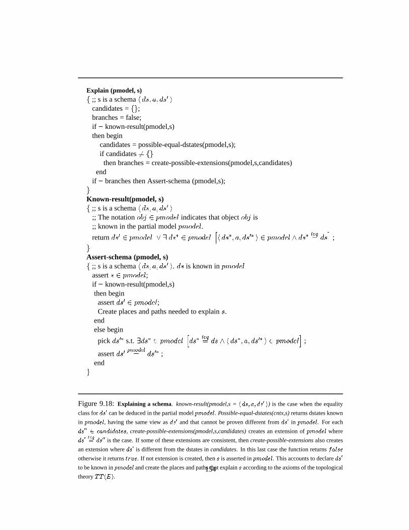
Explain (pmodel, s)f ;; s is a schemah ds; a; ds0 i

candidates =fg;branches = false;if : known-result(pmodel,s)then begin

candidates = possible-equal-dstates(pmodel,s);if candidates6= fgthen branches = create-possible-extensions(pmodel,s,candidates)

endif : branches then Assert-schema (pmodel,s);gKnown-result(pmodel, s)f ;; s is a schemah ds; a; ds0 i

;; The notationobj 2 pmodel indicates that objectobj is;; known in the partial modelpmodel.

returnds0 2 pmodel _ 9 ds� 2 pmodelhh ds�; a; ds0� i 2 pmodel ^ ds�

teq= ds

i;

gAssert-schema (pmodel, s)f ;; s is a schemah ds; a; ds0 i. ds is known inpmodel

asserts 2 pmodel;if : known-result(pmodel,s)then beginassertds0 2 pmodel;Create places and paths needed to explains.

endelse begin

pick ds0� s.t.9ds� 2 pmodelhds�

teq= ds ^ h ds�; a; ds0� i 2 pmodel

i;

assertds0pmodel= ds0� ;

endg

Figure 9.18:Explaining a schema. known-result(pmodel,s =h ds; a; ds0 i) is the case when the equality

class fords0 can be deduced in the partial modelpmodel. Possible-equal-dstates(cntx,s)returns dstates known

in pmodel, having the same view asds0 and that cannot be proven different fromds0 in pmodel. For each

ds00 2 candidates, create-possible-extensions(pmodel,s,candidates)creates an extension ofpmodel where

ds0teq= ds00 is the case. If some of these extensions are consistent, thencreate-possible-extensionsalso creates

an extension whereds0 is different from the dstates incandidates. In this last case the function returnsfalse

otherwise it returnstrue. If not extension is created, thens is asserted inpmodel. This accounts to declareds0

to be known inpmodel and create the places and paths that explains according to the axioms of the topological

theoryTT (E).154

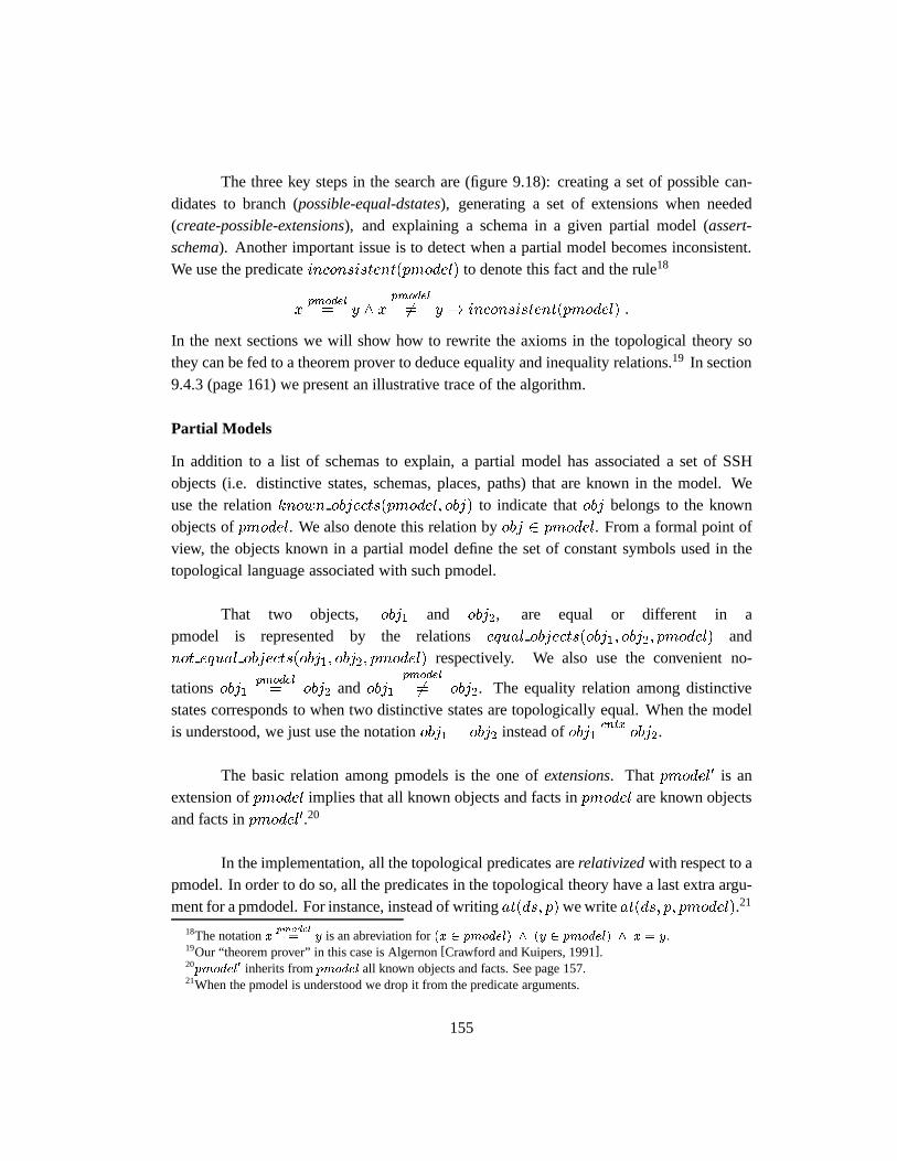
The three key steps in the search are (figure 9.18): creating a set of possible can-didates to branch (possible-equal-dstates), generating a set of extensions when needed(create-possible-extensions), and explaining a schema in a given partial model (assert-schema). Another important issue is to detect when a partial model becomes inconsistent.We use the predicateinconsistent(pmodel) to denote this fact and the rule18

xpmodel= y ^ x

pmodel

6= y ! inconsistent(pmodel) :

In the next sections we will show how to rewrite the axioms in the topological theory sothey can be fed to a theorem prover to deduce equality and inequality relations.19 In section9.4.3 (page 161) we present an illustrative trace of the algorithm.

Partial Models

In addition to a list of schemas to explain, a partial model has associated a set of SSHobjects (i.e. distinctive states, schemas, places, paths) that are known in the model. Weuse the relationknown objects(pmodel; obj) to indicate thatobj belongs to the knownobjects ofpmodel. We also denote this relation byobj 2 pmodel. From a formal point ofview, the objects known in a partial model define the set of constant symbols used in thetopological language associated with such pmodel.

That two objects, obj1 and obj2, are equal or different in apmodel is represented by the relationsequal objects(obj1; obj2; pmodel) andnot equal objects(obj1; obj2; pmodel) respectively. We also use the convenient no-

tationsobj1pmodel= obj2 and obj1

pmodel

6= obj2. The equality relation among distinctivestates corresponds to when two distinctive states are topologically equal. When the modelis understood, we just use the notationobj1 = obj2 instead ofobj1

cntx= obj2.

The basic relation among pmodels is the one ofextensions. That pmodel0 is anextension ofpmodel implies that all known objects and facts inpmodel are known objectsand facts inpmodel0.20

In the implementation, all the topological predicates arerelativizedwith respect to apmodel. In order to do so, all the predicates in the topological theory have a last extra argu-ment for a pmdodel. For instance, instead of writingat(ds; p)we writeat(ds; p; pmodel).21

18The notationxpmodel= y is an abreviation for(x 2 pmodel) ^ (y 2 pmodel) ^ x = y.

19Our “theorem prover” in this case is Algernon[Crawford and Kuipers, 1991].20pmodel0 inherits frompmodel all known objects and facts. See page 157.21When the pmodel is understood we drop it from the predicate arguments.

155

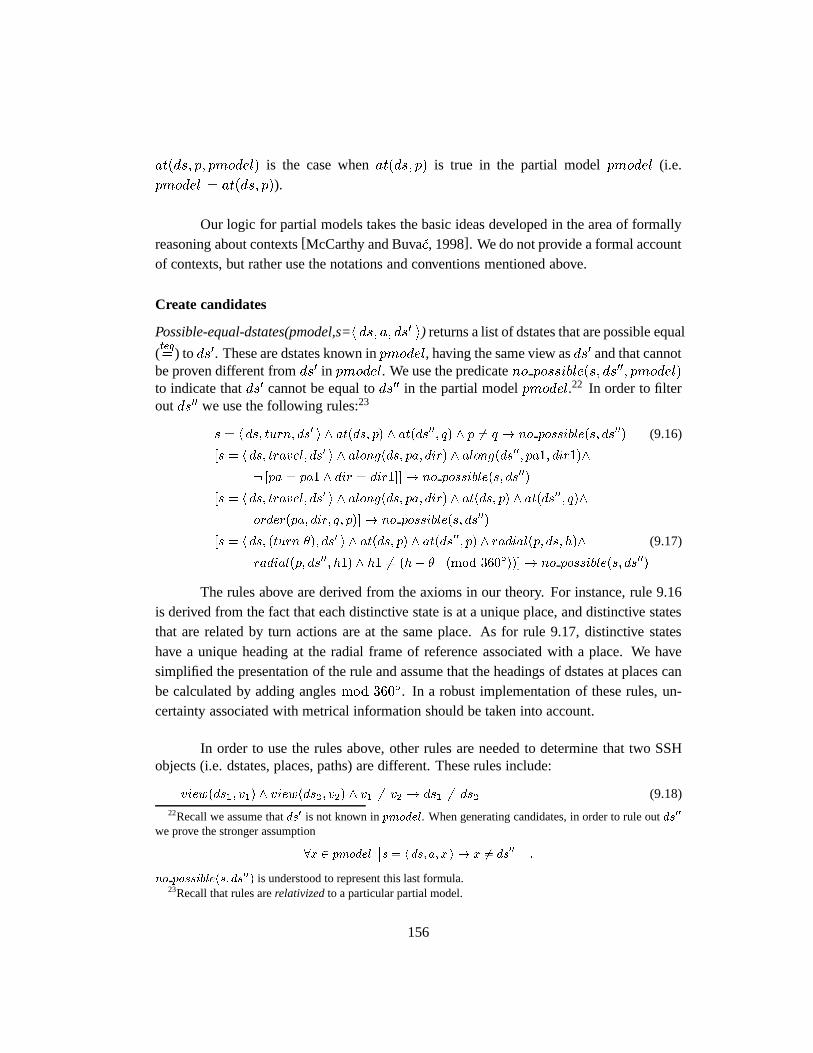
at(ds; p; pmodel) is the case whenat(ds; p) is true in the partial modelpmodel (i.e.pmodel j= at(ds; p)).

Our logic for partial models takes the basic ideas developed in the area of formallyreasoning about contexts[McCarthy and Buva�c, 1998]. We do not provide a formal accountof contexts, but rather use the notations and conventions mentioned above.

Create candidates

Possible-equal-dstates(pmodel,s=h ds; a; ds0 i) returns a list of dstates that are possible equal

(teq= ) tods0. These are dstates known inpmodel, having the same view asds0 and that cannot

be proven different fromds0 in pmodel. We use the predicateno possible(s; ds00; pmodel)to indicate thatds0 cannot be equal tods00 in the partial modelpmodel.22 In order to filteroutds00 we use the following rules:23

s = h ds; turn; ds0 i ^ at(ds; p) ^ at(ds00; q) ^ p 6= q ! no possible(s; ds00) (9.16)

[s = h ds; travel; ds0 i ^ along(ds; pa; dir) ^ along(ds00; pa1; dir1)^

: [pa = pa1 ^ dir = dir1]]! no possible(s; ds00)

[s = h ds; travel; ds0 i ^ along(ds; pa; dir) ^ at(ds; p) ^ at(ds00; q)^

order(pa; dir; q; p)]! no possible(s; ds00)

[s = h ds; (turn �); ds0 i ^ at(ds; p) ^ at(ds00; p) ^ radial(p; ds; h)^ (9.17)

radial(p; ds00; h1) ^ h1 6= (h+ � (mod 360Æ))]! no possible(s; ds00)

The rules above are derived from the axioms in our theory. For instance, rule 9.16is derived from the fact that each distinctive state is at a unique place, and distinctive statesthat are related by turn actions are at the same place. As for rule 9.17, distinctive stateshave a unique heading at the radial frame of reference associated with a place. We havesimplified the presentation of the rule and assume that the headings of dstates at places canbe calculated by adding anglesmod 360Æ. In a robust implementation of these rules, un-certainty associated with metrical information should be taken into account.

In order to use the rules above, other rules are needed to determine that two SSHobjects (i.e. dstates, places, paths) are different. These rules include:

view(ds1; v1) ^ view(ds2; v2) ^ v1 6= v2 ! ds1 6= ds2 (9.18)22Recall we assume thatds0 is not known inpmodel. When generating candidates, in order to rule outds00

we prove the stronger assumption

8x 2 pmodel�s = h ds; a; x i ! x 6= ds

00�

:

no possible(s; ds00) is understood to represent this last formula.23Recall that rules arerelativizedto a particular partial model.

156

h ds; turn; ds0 i ! ds 6= ds0 (9.19)

order(pa; dir; p; q) ! p 6= q (9.20)

radial(p; ds1; h1) ^ radial(p; ds2; h2) ^ h1 6= h2! ds1 6= ds2 (9.21)

position1(pa; dir; p1; pos1)^ position1(pa; dir; p2; pos2)^pos1 6=pos2! p1 6=p2 (9.22)

LeftOf(pa; dir; p) ^ on(pa; q)! p 6= q (9.23)

LeftOf(pa; dir; p) ^ on(pa1; p)! pa 6= pa1 (9.24)

Rules 9.18 and 9.19 rely on our basic assumption that dstates have a unique viewand turn actions link different distinctive states. Rule 9.20 uses the fact that paths are notcircular in order to conclude that ifp is beforeq thenp andq must be different. Rules9.21 and 9.22 use radial and one dimensional frames of reference to conclude inequalityof dstates and places, respectively. Rules 9.23 and 9.24 use boundary relations in order todistinguish places and paths respectively.24

Finally, rules to prove equality among SSH objects include:

at(ds; p) ^ at(ds; q)! p = q (9.25)

along(ds; pa; dir) ^ along(ds; pa1; dir1)! pa = pa1 ^ dir = dir1 (9.26)

The rules to derive equality and inequality relations are not necessarilycompleteinthe following sense. It is possible thatno possible(s; ds00) cannot be proved, and sods00

will be a valid candidate. A new extension ofpmodel will be created in whichds0teq= ds00 is

asserted. However, when assertings in that extension, it can then be proved thatds0teq

6= ds00.We further discuss this issue in the next section.

Creating extensions

For eachds0i 2 candidates, create-possible-extensions(pmodel,s=h ds; a; ds0 i,candidates)

creates a possible extension forpmodel whereds0teq= ds0i is the case. If some of these ex-

tensions are consistent, thencreate-possible-extensionsalso creates an extension whereds0

is known and different from the dstates incandidates. In this last case the function returns24In Algernon[Crawford and Kuipers, 1991] some of these rules are implemented asforward-chaining (if-

added)rules (e.g. rules 9.18 and 9.19) and others asbackward-chaining (if-needed) rules(e.g. rules 9.23and 9.24). The problem with if-added rules is that they could derive a large number of useless truths. Forinstance, if rule 9.23 were implemented as an if-added rule, Algernon’s engine will prove that placesp andqare different for any placeq on a pathpa and placep to the left ofpa. While this is the case, in general we wantto use boundary relations to derive inequalities among particular pairs of places rather than indiscriminatelybetween all pair of places. Algernon should not (try to) prove at front inequalities among all places in the map!.We provide no further discussion on this issue which applies in general to rule base systems that use forwardchaining rules.

157

false otherwise it returnstrue.

Givends0i 2 candidates, a new extensionpmodel0i is created whereds0pmodel0

i= ds0i

is the case. In addition,ds0pmodel0i6= ds0j is also asserted fords0j 2 candidates; ds0j 6= ds0i.

The extension(pmodel; pmodel0i) relation among partial models is then asserted. Thatpmodel0i is an extension ofpmodel implies that all known objects and facts inpmodel

are known objects and facts inpmodel0i. This inheritance property of extensions can beimplemented in Algernon by rules like the next ones:

extension(pmodel; pmodel1)^ known objects(pmodel; obj)

! known objects(pmodel1; ojb)

extension(pmodel; pmodel1)^ equal objects(pmodel; obj1; obj2)

! equal objects(pmodel1; obj1; obj2)

extension(pmodel; pmodel1)^ not equal objects(pmodel; obj1; obj2)

! not equal objects(pmodel1; obj1; obj2)

at(ds; place; pmodel)^ extension(pmodel; pmodel1)! at(ds; place; pmodel1)

: : :

In addition to state thatextension(pmodel; pmodel0i) is the case,s becomes thenext schema that has to be explained bypmodel0i. It is possible that by explainings at thispoint (by assertings in pmodel0i), pmodel0i becomes inconsistent and so it should not beconsidered further in the search.25 Shouldpmodel0i become inconsistent, then one has todelete theextension(pmodel; pmodel0i) relation. We calllook aheadto this extra step ofexplainings in pmodel0i (see figure 9.19).

Assert schema

Assert-schema(pmodel, s)creates the places and paths needed to explains. An example ofthe rules used to explains is presented in figure 9.20.

Instead of assertings = h ds; a; ds0 i in pmodel, the algorithm assertss� = h ds�; a; ds0� i

whereds� and ds0� are theteq= representatives for the equality classes ofds and ds0 in

pmodel. Asserting a schema in Algernon corresponds to creating the frame (object) repre-senting the schema. Forward and backward chaining rules derived from the SSH topologicaltheory are then evaluated, and places and paths needed to explains are created (see figure9.20).

25This could be the case since rules to filter out candidates may not be complete. See previous section.

158

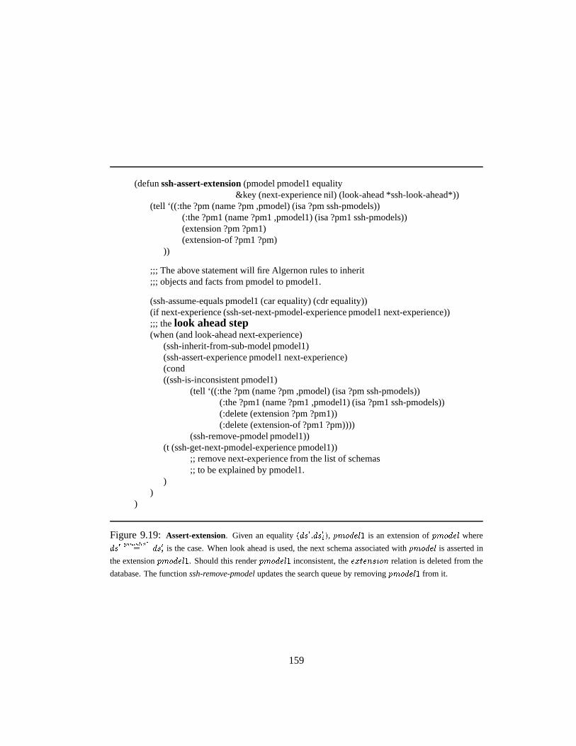
(defunssh-assert-extension(pmodel pmodel1 equality&key (next-experience nil) (look-ahead *ssh-look-ahead*))

(tell ‘((:the ?pm (name ?pm ,pmodel) (isa ?pm ssh-pmodels))(:the ?pm1 (name ?pm1 ,pmodel1) (isa ?pm1 ssh-pmodels))(extension ?pm ?pm1)(extension-of ?pm1 ?pm)

))

;;; The above statement will fire Algernon rules to inherit;;; objects and facts from pmodel to pmodel1.

(ssh-assume-equals pmodel1 (car equality) (cdr equality))(if next-experience (ssh-set-next-pmodel-experience pmodel1 next-experience));;; thelook ahead step(when (and look-ahead next-experience)

(ssh-inherit-from-sub-model pmodel1)(ssh-assert-experience pmodel1 next-experience)(cond((ssh-is-inconsistent pmodel1)

(tell ‘((:the ?pm (name ?pm ,pmodel) (isa ?pm ssh-pmodels))(:the ?pm1 (name ?pm1 ,pmodel1) (isa ?pm1 ssh-pmodels))(:delete (extension ?pm ?pm1))(:delete (extension-of ?pm1 ?pm))))

(ssh-remove-pmodel pmodel1))(t (ssh-get-next-pmodel-experience pmodel1))

;; remove next-experience from the list of schemas;; to be explained by pmodel1.

))

)

Figure 9.19:Assert-extension. Given an equality(ds0:ds0i), pmodel1 is an extension ofpmodel where

ds0pmodel1

= ds0i is the case. When look ahead is used, the next schema associated withpmodel is asserted in

the extensionpmodel1. Should this renderpmodel1 inconsistent, theextension relation is deleted from the

database. The functionssh-remove-pmodelupdates the search queue by removingpmodel1 from it.

159

(defunssh-assert-experience(pmodel e)(let ( schema ds-context ds-result act)

(setf schema(first (ask ‘((:the ?e (name ?e ,e) (isa ?e experiences))

(E-context-ds ?e ?ds) (E-result-ds ?e ?ds1) (E-action ?e ?a)):collect ’(?ds ?a ?ds1))))

(setf ds-context (ssh-find-or-create-equal pmodel (first schema)))(setf ds-result (ssh-find-or-create-equal pmodel (third schema)))

;;; ssh-find-or-create-equal will ensure that ?ds and ?ds1 are known in pmodel

(setf act (second schema))(create-schema :pmodel pmodel

:initial-ds ds-context :result-ds ds-result:action act)

)

(defunCreate-Schema(&key (pmodel nil)(action nil)(initial-ds nil) (result-ds nil))

;; create frame representing schemahinitial-ds, action, result-dsi.)

;;; Example of Algernon rules used to explain schemas.

(tell ’((:rules Schemas((S-action ?s ?a) (A-type ?a turn) (S-context-ds ?s ?dsc ?cntx)

(S-result-ds ?s ?dsr ?pmodel)(at ?dsc ?p ?pmodel) ;;; create place if necessary! ;;; turning keeps the agent in the same place(at ?dsr ?p ?pmodel)

))’((:rules distinctive-states

((at ?ds ?p ?pmodel) ;;; a distinctive state is always at a place;;; check that ?ds is not at a place already(:fail (:boundp ?p)) (:boundp ?pmodel) (:fail (:retrieve (at ?ds ?a-p ?pmodel)));;; if so then create place(:bind ?p (Create-place (ssh-create-place-name) :pmodel ’?pmodel))

)))

Figure 9.20:Asserting a schema in Algernon corresponds to creating the frame (object) representing the

schema. Forward and backward chaining rules derived from the SSH topological axioms will then be evaluated,

and places and paths needed to explains will be created (if needed).

160

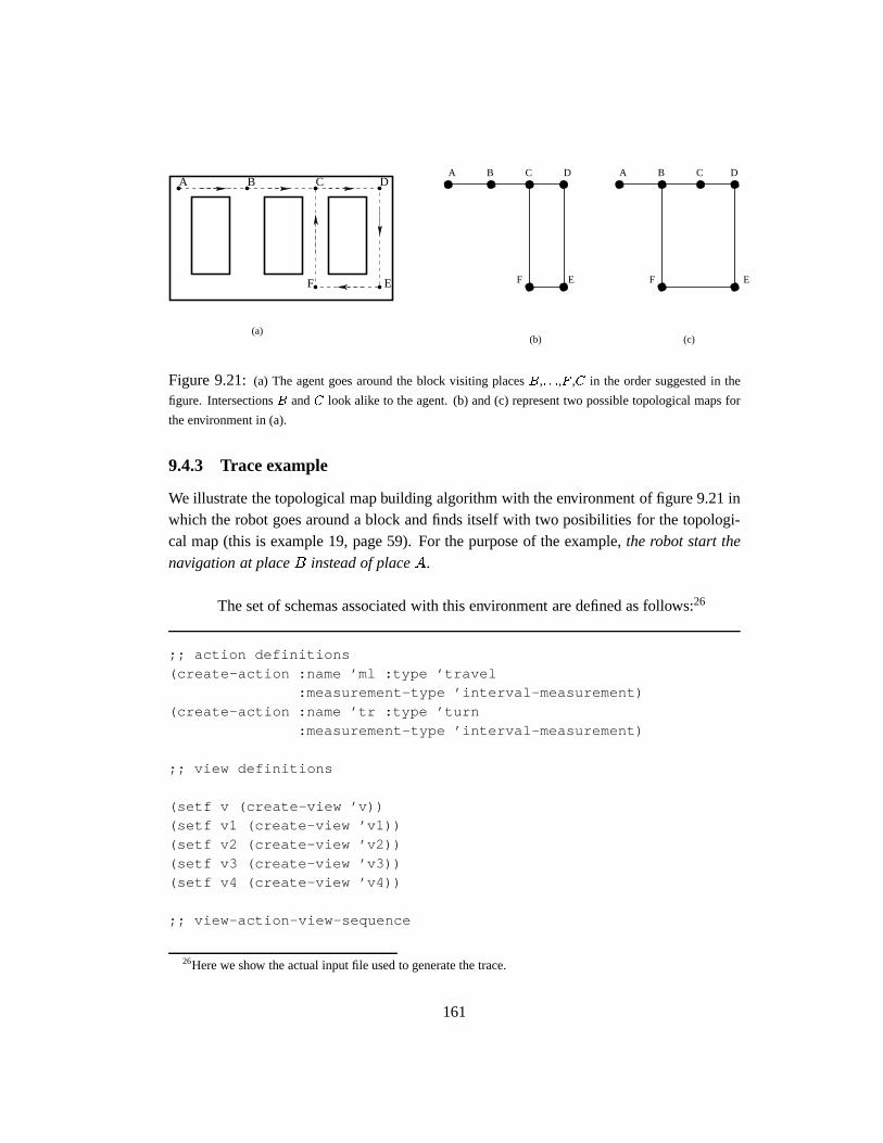
EF

B C DAA C D

EF

A C

(a)(b) (c)

B B D

EF

Figure 9.21:(a) The agent goes around the block visiting placesB,: : :,F ,C in the order suggested in the

figure. IntersectionsB andC look alike to the agent. (b) and (c) represent two possible topological maps for

the environment in (a).

9.4.3 Trace example

We illustrate the topological map building algorithm with the environment of figure 9.21 inwhich the robot goes around a block and finds itself with two posibilities for the topologi-cal map (this is example 19, page 59). For the purpose of the example,the robot start thenavigation at placeB instead of placeA.

The set of schemas associated with this environment are defined as follows:26

;; action definitions

(create-action :name ’ml :type ’travel:measurement-type ’interval-measurement)

(create-action :name ’tr :type ’turn

:measurement-type ’interval-measurement)

;; view definitions

(setf v (create-view ’v))(setf v1 (create-view ’v1))

(setf v2 (create-view ’v2))

(setf v3 (create-view ’v3))(setf v4 (create-view ’v4))

;; view-action-view-sequence

26Here we show the actual input file used to generate the trace.

161

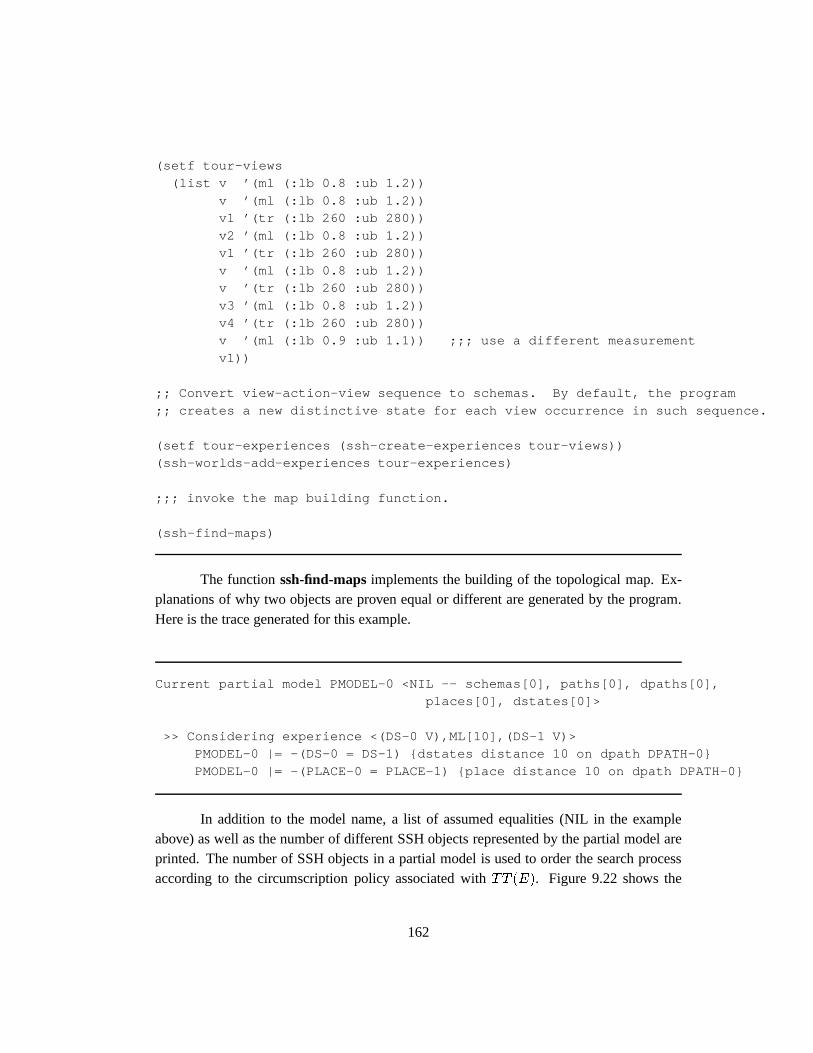
(setf tour-views

(list v ’(ml (:lb 0.8 :ub 1.2))

v ’(ml (:lb 0.8 :ub 1.2))v1 ’(tr (:lb 260 :ub 280))

v2 ’(ml (:lb 0.8 :ub 1.2))v1 ’(tr (:lb 260 :ub 280))

v ’(ml (:lb 0.8 :ub 1.2))v ’(tr (:lb 260 :ub 280))

v3 ’(ml (:lb 0.8 :ub 1.2))

v4 ’(tr (:lb 260 :ub 280))v ’(ml (:lb 0.9 :ub 1.1)) ;;; use a different measurement

v1))

;; Convert view-action-view sequence to schemas. By default, the program

;; creates a new distinctive state for each view occurrence in such sequence.

(setf tour-experiences (ssh-create-experiences tour-views))(ssh-worlds-add-experiences tour-experiences)

;;; invoke the map building function.

(ssh-find-maps)

The functionssh-find-mapsimplements the building of the topological map. Ex-planations of why two objects are proven equal or different are generated by the program.Here is the trace generated for this example.

Current partial model PMODEL-0 <NIL -- schemas[0], paths[0], dpaths[0],places[0], dstates[0]>

>> Considering experience <(DS-0 V),ML[10],(DS-1 V)>PMODEL-0 |= -(DS-0 = DS-1) {dstates distance 10 on dpath DPATH-0}

PMODEL-0 |= -(PLACE-0 = PLACE-1) {place distance 10 on dpath DPATH-0}

In addition to the model name, a list of assumed equalities (NIL in the exampleabove) as well as the number of different SSH objects represented by the partial model areprinted. The number of SSH objects in a partial model is used to order the search processaccording to the circumscription policy associated withTT (E). Figure 9.22 shows the

162

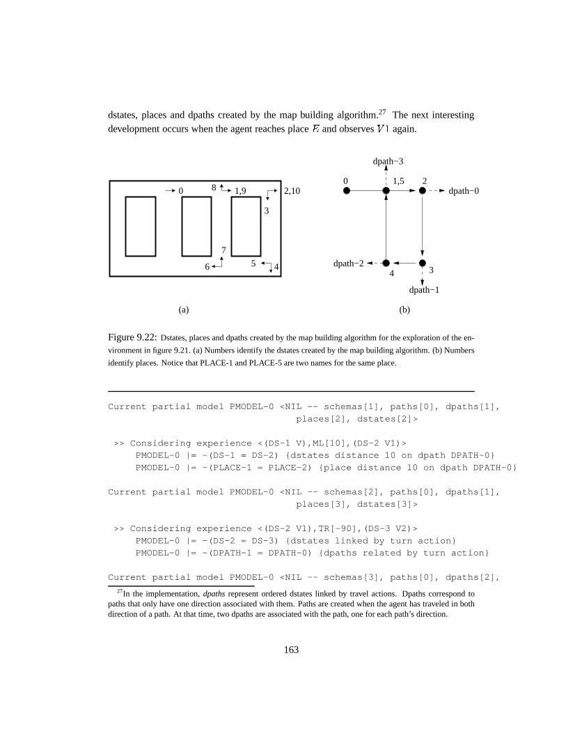
dstates, places and dpaths created by the map building algorithm.27 The next interestingdevelopment occurs when the agent reaches placeE and observesV 1 again.

0 1,9

3

56

7

8 2,10

4

0 2dpath−0

dpath−1

dpath−23

dpath−3

4

1,5

(b)(a)

Figure 9.22:Dstates, places and dpaths created by the map building algorithm for the exploration of the en-

vironment in figure 9.21. (a) Numbers identify the dstates created by the map building algorithm. (b) Numbers

identify places. Notice that PLACE-1 and PLACE-5 are two names for the same place.

Current partial model PMODEL-0 <NIL -- schemas[1], paths[0], dpaths[1],

places[2], dstates[2]>

>> Considering experience <(DS-1 V),ML[10],(DS-2 V1)>PMODEL-0 |= -(DS-1 = DS-2) {dstates distance 10 on dpath DPATH-0}

PMODEL-0 |= -(PLACE-1 = PLACE-2) {place distance 10 on dpath DPATH-0}

Current partial model PMODEL-0 <NIL -- schemas[2], paths[0], dpaths[1],

places[3], dstates[3]>

>> Considering experience <(DS-2 V1),TR[-90],(DS-3 V2)>

PMODEL-0 |= -(DS-2 = DS-3) {dstates linked by turn action}PMODEL-0 |= -(DPATH-1 = DPATH-0) {dpaths related by turn action}

Current partial model PMODEL-0 <NIL -- schemas[3], paths[0], dpaths[2],

27In the implementation,dpathsrepresent ordered dstates linked by travel actions. Dpaths correspond topaths that only have one direction associated with them. Paths are created when the agent has traveled in bothdirection of a path. At that time, two dpaths are associated with the path, one for each path’s direction.

163

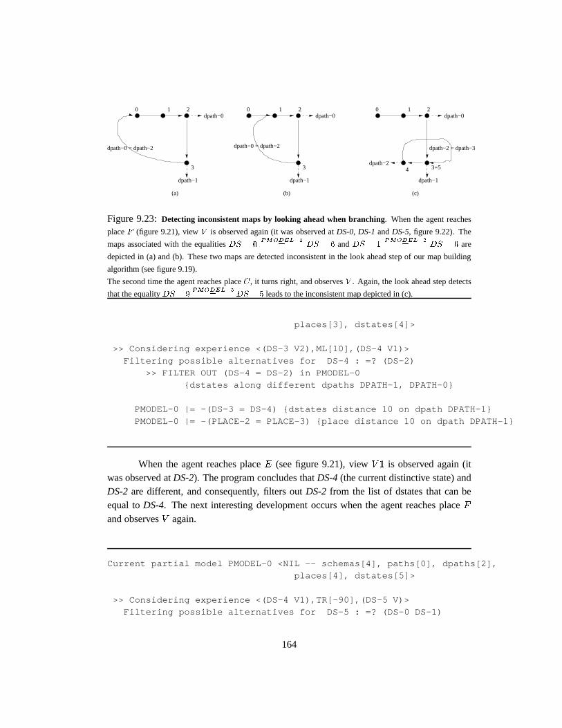
0 2dpath−0

dpath−1

3

0 2dpath−0

dpath−1

3

(b)

dpath−0 = dpath−2dpath−0 = dpath−2

0 2dpath−0

dpath−1

dpath−24

dpath−2 = dpath−3

3=5

(c)(a)

1 1 1

Figure 9.23:Detecting inconsistent maps by looking ahead when branching. When the agent reaches

placeF (figure 9.21), viewV is observed again (it was observed atDS-0, DS-1andDS-5, figure 9.22). The

maps associated with the equalitiesDS � 0PMODEL�1

= DS � 6 andDS � 1PMODEL�2

= DS � 6 are

depicted in (a) and (b). These two maps are detected inconsistent in the look ahead step of our map building

algorithm (see figure 9.19).

The second time the agent reaches placeC, it turns right, and observesV . Again, the look ahead step detects

that the equalityDS � 9PMODEL�5

= DS � 5 leads to the inconsistent map depicted in (c).

places[3], dstates[4]>

>> Considering experience <(DS-3 V2),ML[10],(DS-4 V1)>

Filtering possible alternatives for DS-4 : =? (DS-2)

>> FILTER OUT (DS-4 = DS-2) in PMODEL-0{dstates along different dpaths DPATH-1, DPATH-0}

PMODEL-0 |= -(DS-3 = DS-4) {dstates distance 10 on dpath DPATH-1}

PMODEL-0 |= -(PLACE-2 = PLACE-3) {place distance 10 on dpath DPATH-1}

When the agent reaches placeE (see figure 9.21), viewV 1 is observed again (itwas observed atDS-2). The program concludes thatDS-4(the current distinctive state) andDS-2are different, and consequently, filters outDS-2 from the list of dstates that can beequal toDS-4. The next interesting development occurs when the agent reaches placeF

and observesV again.

Current partial model PMODEL-0 <NIL -- schemas[4], paths[0], dpaths[2],places[4], dstates[5]>

>> Considering experience <(DS-4 V1),TR[-90],(DS-5 V)>Filtering possible alternatives for DS-5 : =? (DS-0 DS-1)

164

PMODEL-0 |= -(PLACE-3 = PLACE-0)

{PLACE-3 is to the right of DPATH-0, PLACE-0 is on dpath DPATH-0}

>> FILTER OUT (DS-5 = DS-0) in PMODEL-0{dstates at different places PLACE-3, PLACE-0}

PMODEL-0 |= -(PLACE-3 = PLACE-1){PLACE-3 is to the right of DPATH-0, PLACE-1 is on dpath DPATH-0}

>> FILTER OUT (DS-5 = DS-1) in PMODEL-0{dstates at different places PLACE-3, PLACE-1}

PMODEL-0 |= -(DS-4 = DS-5) {dstates linked by turn action}

PMODEL-0 |= -(DPATH-2 = DPATH-1) {dpaths related by turn action}

Current partial model PMODEL-0 <NIL -- schemas[5], paths[0], dpaths[3],places[4], dstates[6]>

>> Considering experience <(DS-5 V),ML[10],(DS-6 V)>Filtering possible alternatives for DS-6 : =? (DS-0 DS-1 DS-5)

>> FILTER OUT (DS-6 = DS-5) in PMODEL-0{DS-5 is before DS-6 in dpath DPATH-2}

>> Creating possible extensions

- PMODEL-0 + {DS-0 = DS-6} --> PMODEL-1

PMODEL-1 |= DPATH-0 = DPATH-2 {dstate DS-0 along both dpaths}PMODEL-1 |= DPATH-2 = DPATH-0 {dstate DS-5 along both dpaths}

PMODEL-1 |= -(DPATH-0 = DPATH-2){PLACE-3 is to the right of DPATH-0 and on dpath DPATH-2}

LOOK AHEAD --> PMODEL-1 **** INCONSISTENT ****

- PMODEL-0 + {DS-1 = DS-6} --> PMODEL-2

PMODEL-2 |= DPATH-0 = DPATH-2 {dstate DS-1 along both dpaths}

PMODEL-2 |= DPATH-2 = DPATH-0 {dstate DS-5 along both dpaths}PMODEL-2 |= -(DPATH-0 = DPATH-2)

{PLACE-3 is to the right of DPATH-0 and on dpath DPATH-2}

LOOK AHEAD --> PMODEL-2 **** INCONSISTENT ****

PMODEL-0 |= -(PLACE-3 = PLACE-4) {place distance 10 on dpath DPATH-2}

When the agent reaches placeF (see figure 9.21), viewV is observed again (it wasobserved atDS-0, DS-1andDS-5) at dstateDS-6. The program deduces thatDS-6 is dif-ferent fromDS-5. Two extensions ofPMODEL-0are created to explore the possibilities

165

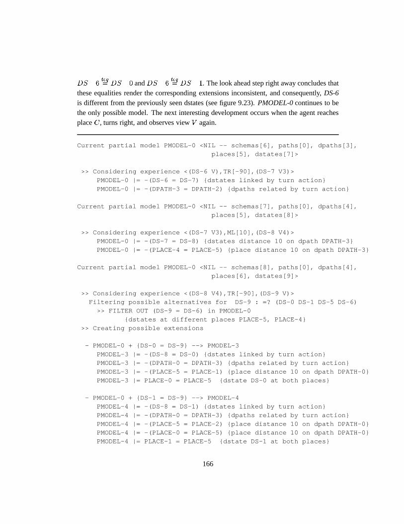
DS�6teq= DS�0 andDS�6

teq= DS�1. The look ahead step right away concludes that

these equalities render the corresponding extensions inconsistent, and consequently,DS-6is different from the previously seen dstates (see figure 9.23).PMODEL-0continues to bethe only possible model. The next interesting development occurs when the agent reachesplaceC, turns right, and observes viewV again.

Current partial model PMODEL-0 <NIL -- schemas[6], paths[0], dpaths[3],places[5], dstates[7]>

>> Considering experience <(DS-6 V),TR[-90],(DS-7 V3)>

PMODEL-0 |= -(DS-6 = DS-7) {dstates linked by turn action}

PMODEL-0 |= -(DPATH-3 = DPATH-2) {dpaths related by turn action}

Current partial model PMODEL-0 <NIL -- schemas[7], paths[0], dpaths[4],places[5], dstates[8]>

>> Considering experience <(DS-7 V3),ML[10],(DS-8 V4)>PMODEL-0 |= -(DS-7 = DS-8) {dstates distance 10 on dpath DPATH-3}

PMODEL-0 |= -(PLACE-4 = PLACE-5) {place distance 10 on dpath DPATH-3}

Current partial model PMODEL-0 <NIL -- schemas[8], paths[0], dpaths[4],places[6], dstates[9]>

>> Considering experience <(DS-8 V4),TR[-90],(DS-9 V)>Filtering possible alternatives for DS-9 : =? (DS-0 DS-1 DS-5 DS-6)

>> FILTER OUT (DS-9 = DS-6) in PMODEL-0{dstates at different places PLACE-5, PLACE-4}

>> Creating possible extensions

- PMODEL-0 + {DS-0 = DS-9} --> PMODEL-3

PMODEL-3 |= -(DS-8 = DS-0) {dstates linked by turn action}PMODEL-3 |= -(DPATH-0 = DPATH-3) {dpaths related by turn action}

PMODEL-3 |= -(PLACE-5 = PLACE-1) {place distance 10 on dpath DPATH-0}

PMODEL-3 |= PLACE-0 = PLACE-5 {dstate DS-0 at both places}

- PMODEL-0 + {DS-1 = DS-9} --> PMODEL-4PMODEL-4 |= -(DS-8 = DS-1) {dstates linked by turn action}

PMODEL-4 |= -(DPATH-0 = DPATH-3) {dpaths related by turn action}

PMODEL-4 |= -(PLACE-5 = PLACE-2) {place distance 10 on dpath DPATH-0}PMODEL-4 |= -(PLACE-0 = PLACE-5) {place distance 10 on dpath DPATH-0}

PMODEL-4 |= PLACE-1 = PLACE-5 {dstate DS-1 at both places}

166

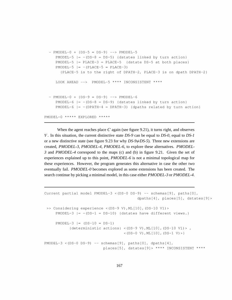
- PMODEL-0 + {DS-5 = DS-9} --> PMODEL-5

PMODEL-5 |= -(DS-8 = DS-5) {dstates linked by turn action}PMODEL-5 |= PLACE-3 = PLACE-5 {dstate DS-5 at both places}

PMODEL-5 |= -(PLACE-5 = PLACE-3){PLACE-5 is to the right of DPATH-2, PLACE-3 is on dpath DPATH-2}

LOOK AHEAD --> PMODEL-5 **** INCONSISTENT ****

- PMODEL-0 + {DS-9 = DS-9} --> PMODEL-6

PMODEL-6 |= -(DS-8 = DS-9) {dstates linked by turn action}PMODEL-6 |= -(DPATH-4 = DPATH-3) {dpaths related by turn action}

PMODEL-0 ***** EXPLORED *****

When the agent reaches placeC again (see figure 9.21), it turns right, and observesV . In this situation, the current distinctive stateDS-9can be equal toDS-0, equal toDS-1or a new distinctive state (see figure 9.23 for whyDS-96=DS-5). Three new extensions arecreated,PMODEL-3, PMODEL-4, PMODEL-6, to explore these alternatives.PMODEL-3 and PMODEL-4correspond to the maps (c) and (b) in figure 9.21. Given the set ofexperiences explained up to this point,PMODEL-6 is not a minimal topological map forthese experiences. However, the program generates this alternative in case the other twoeventually fail. PMODEL-0becomes explored as some extensions has been created. Thesearch continue by picking a minimal model, in this case eitherPMODEL-3or PMODEL-4.

Current partial model PMODEL-3 <(DS-0 DS-9) -- schemas[9], paths[0],

dpaths[4], places[5], dstates[9]>

>> Considering experience <(DS-9 V),ML[10],(DS-10 V1)>

PMODEL-3 |= -(DS-1 = DS-10) {dstates have different views.}

PMODEL-3 |= (DS-10 = DS-1){deterministic actions: <(DS-9 V),ML[10],(DS-10 V1)> ,

<(DS-0 V),ML[10],(DS-1 V)>}

PMODEL-3 <(DS-0 DS-9) -- schemas[9], paths[0], dpaths[4],

places[5], dstates[9]> **** INCONSISTENT ****

167

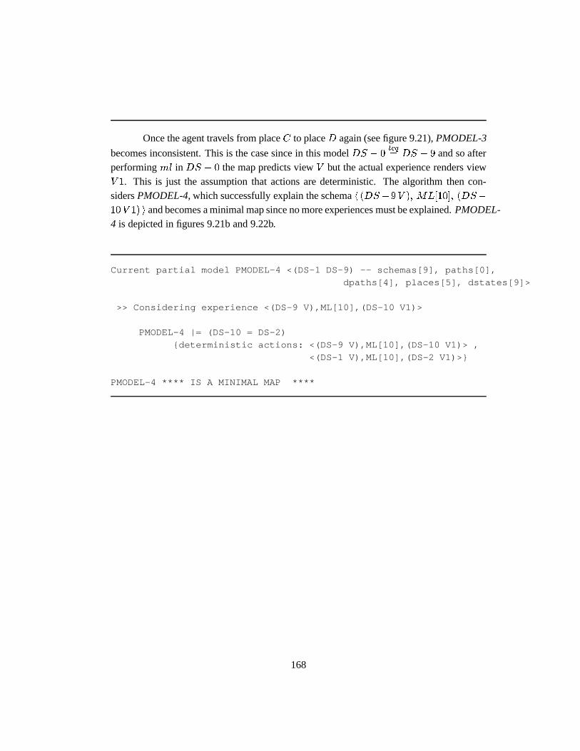
Once the agent travels from placeC to placeD again (see figure 9.21),PMODEL-3

becomes inconsistent. This is the case since in this modelDS � 0teq= DS � 9 and so after

performingml in DS � 0 the map predicts viewV but the actual experience renders viewV 1. This is just the assumption that actions are deterministic. The algorithm then con-sidersPMODEL-4, which successfully explain the schemah (DS�9V ); ML[10]; (DS�

10V 1) i and becomes a minimal map since no more experiences must be explained.PMODEL-4 is depicted in figures 9.21b and 9.22b.

Current partial model PMODEL-4 <(DS-1 DS-9) -- schemas[9], paths[0],

dpaths[4], places[5], dstates[9]>

>> Considering experience <(DS-9 V),ML[10],(DS-10 V1)>

PMODEL-4 |= (DS-10 = DS-2)

{deterministic actions: <(DS-9 V),ML[10],(DS-10 V1)> ,

<(DS-1 V),ML[10],(DS-2 V1)>}

PMODEL-4 **** IS A MINIMAL MAP ****

168

9.5 Map building examples

In this section we describe two examples where a physical robot (Vulcan) builds a SSH map.The purpose of these examples is to illustrate how the concepts in the previous section applyin office like environments. The first example (Section 9.5.1), shows how the agent usingthe concept of boundary regions can distinguish otherwise identical distinctive states. In thesecond example (Section 9.5.2), Vulcan explores Taylor’s second floor defining distinctivestates at the different corridor intersections.

9.5.1 Rectangular environment

This section shows the SSH map learned by the wheelchair (Vulcan) while exploring a sym-metric environment (namely, a rectangular room). Symmetric environments are particularlydifficult to handle as the same view might occur at different distinctive states, and the SSHcausal level is not enough to distinguish some distinctive states. By using topological andmetrical information the agent can distinguish the different places of the environment.

The environment to explore is a 3m� 8m rectangle, as illustrated in Figure 9.24.The exploration strategy was set to execute a forward action when possible, otherwise turnright, and stop when back to a previously visited distinctive state. Notice that the explorationstrategy is defined in terms of the causal language actionsForward andTurn Right. Therobot chose the most appropriate control law associated with the causal command, whichin this case werefollow left wall andalign to the right w.r.t. the front wallrespectively. Asillustrated in Figure 9.24, different distinctive states look alike (i.e. share the same view).For example, distinctive statesDS-1andDS-5share the same viewVIEW-1.

169

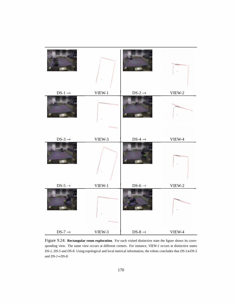
DS-1! VIEW-1 DS-2! VIEW-2

DS-3! VIEW-3 DS-4! VIEW-4

DS-5! VIEW-1 DS-6! VIEW-2

DS-7! VIEW-3 DS-8! VIEW-4

Figure 9.24:Rectangular room exploration. For each visited distinctive state the figure shows its corre-

sponding view. The same view occurs at different corners. For instance,VIEW-1occurs at distinctive states

DS-1, DS-5andDS-8. Using topological and local metrical information, the robots concludes thatDS-16=DS-5

andDS-1=DS-8.

170

Next we provide a commented trace of the different steps and reasoning the robotused during the exploration. At each step the robot continues the exploration by performingan action (forward or turn right) and identifying a distinctive state once the action is per-formed.

Initially, the robot starts at one of the corners of the environment and creates adistinctive state. Here is the program output associated with this step:

-----------------------------Finding current place.

Finding view.

No matching view.+ Creating new view.

> View found: VIEW-1.Finding distinctive state.

+ Creating new d-state DS-1.

> Distinctive state found: DS-1.> Place found: A.

-----------------------------

Since at this point the robot has no stored views, it gives a new name (VIEW-1) toits current view. A new distinctive state (DS-1) is created and associated with this view.The place at which this distinctive state is located is created and calledA (see Axiom 5.16,page 41).

-----------------------------Performing action: Forward.

Control law: Follow left wallExecuting Follow left wall ... Done.

-----------------------------

Finding current place.Finding view.

No matching view.+ Creating new view.

> View found: VIEW-2.

Finding distinctive state.+ Creating new d-state DS-2.

> Distinctive state found: DS-2.> Place found: B.

-----------------------------

The view observed at this point does not match a known view and consequently anew one is created. Since the view is new, so is the current distinctive state. This is the case

171

since a distinctive state has associated a unique view (Axiom 4.7). A new placeB is createdsince the robot executed a travel action which by definition changes the place the robot is at(Corollary 1, page 46).

-----------------------------

Performing action: Right.Control law: Turn right (ref = front wall)

Executing Turn right (ref = front wall) ... Done.-----------------------------

Finding current place.Finding view.

No matching view.

+ Creating new view.> View found: VIEW-3.

Finding distinctive state.+ Creating new d-state DS-3.

> Distinctive state found: DS-3.

> Place found: B.-----------------------------

Notice that since the robot performed aTurn action, it is still at the same placeB(Axiom 5.17), although at a different distinctive stateDS-3.

-----------------------------

Performing action: Forward.

Control law: Follow left wallExecuting Follow left wall ... Done.

-----------------------------Finding current place.

Finding view.

No matching view.+ Creating new view.

> View found: VIEW-4.Finding distinctive state.

+ Creating new d-state DS-4.

> Distinctive state found: DS-4.> Place found: C.

-----------------------------

Since the robot performed aTravelaction, it is at different place fromB. Since theview is new, it creates a new distinctive state and a new placeC. The robot does not checkwhether it is back atA, since it has not experienced the current view at placeA.

172

-----------------------------

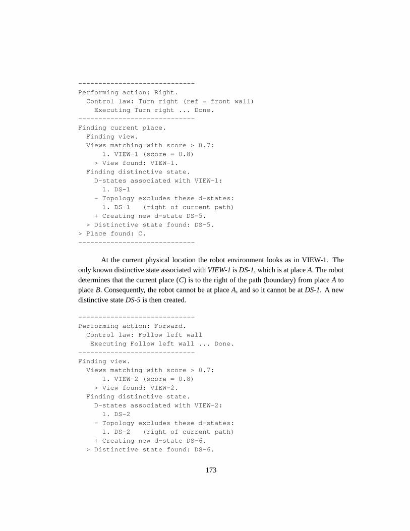
Performing action: Right.

Control law: Turn right (ref = front wall)Executing Turn right ... Done.

-----------------------------Finding current place.

Finding view.Views matching with score > 0.7:

1. VIEW-1 (score = 0.8)

> View found: VIEW-1.Finding distinctive state.

D-states associated with VIEW-1:1. DS-1

- Topology excludes these d-states:

1. DS-1 (right of current path)+ Creating new d-state DS-5.

> Distinctive state found: DS-5.> Place found: C.

-----------------------------

At the current physical location the robot environment looks as in VIEW-1. Theonly known distinctive state associated withVIEW-1is DS-1, which is at placeA. The robotdetermines that the current place (C) is to the right of the path (boundary) from placeA toplaceB. Consequently, the robot cannot be at placeA, and so it cannot be atDS-1. A newdistinctive stateDS-5is then created.

-----------------------------Performing action: Forward.

Control law: Follow left wall

Executing Follow left wall ... Done.-----------------------------

Finding view.Views matching with score > 0.7:

1. VIEW-2 (score = 0.8)

> View found: VIEW-2.Finding distinctive state.

D-states associated with VIEW-2:1. DS-2

- Topology excludes these d-states:1. DS-2 (right of current path)

+ Creating new d-state DS-6.

> Distinctive state found: DS-6.

173

> Place found: D.

-----------------------------

By a reasoning similar to the one used to distinguishDS-1from DS-5, the robot candistinguish the current distinctive state (DS-6) from DS-2. Notice that this time the robotknows that it is not at placeC (since it just traveled from it, lemma 1) and it is not at placeB, since the current place (D) is on the right of the path fromB to C.

-----------------------------Performing action: Right.

Control law: Turn right (ref = front wall)Executing Turn right (ref = front wall) ... Done.

-----------------------------

Finding current place.Finding view.

Views matching with score > 0.7:1. VIEW-3 (score = 0.799264)

> View found: VIEW-3.Finding distinctive state.

D-states associated with VIEW-3:

1. DS-3- Topology excludes these d-states:

1. DS-3 (right of boundary)+ Creating new d-state DS-7.

> Distinctive state found: DS-7.

> Place found: D.

-----------------------------Performing action: Forward.

Control law: Follow left wall

Executing Follow left wall ... Done.-----------------------------

Finding current place.Finding view.

Views matching with score > 0.7:1. VIEW-4 (score = 0.710665)

> View found: VIEW-4.

Finding distinctive state.D-states associated with VIEW-4:

1. DS-4- Topology excludes these d-states:

1. DS-4 (right of current path)

174

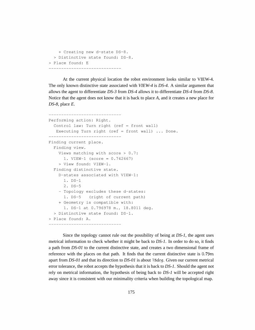
+ Creating new d-state DS-8.

> Distinctive state found: DS-8.

> Place found: E-----------------------------

At the current physical location the robot environment looks similar to VIEW-4.The only known distinctive state associated withVIEW-4is DS-4. A similar argument thatallows the agent to differentiateDS-3from DS-4allows it to differentiateDS-4from DS-8.Notice that the agent does not know that it is back to placeA, and it creates a new place forDS-8, placeE.

-----------------------------Performing action: Right.

Control law: Turn right (ref = front wall)

Executing Turn right (ref = front wall) ... Done.-----------------------------

Finding current place.Finding view.

Views matching with score > 0.7:

1. VIEW-1 (score = 0.742667)> View found: VIEW-1.

Finding distinctive state.D-states associated with VIEW-1:

1. DS-1

2. DS-5- Topology excludes these d-states:

1. DS-5 (right of current path)+ Geometry is compatible with:

1. DS-1 at 0.796978 m., 18.8011 deg.> Distinctive state found: DS-1.

> Place found: A.

-----------------------------

Since the topology cannot rule out the possibility of being atDS-1, the agent usesmetrical information to check whether it might be back toDS-1. In order to do so, it findsa path fromDS-01to the current distinctive state, and creates a two dimensional frame ofreference with the places on that path. It finds that the current distinctive state is0:79m

apart fromDS-01and that its direction toDS-01is about18deg. Given our current metricalerror tolerance, the robot accepts the hypothesis that it is back toDS-1. Should the agent notrely on metrical information, the hypothesis of being back toDS-1will be accepted rightaway since it is consistent with our minimality criteria when building the topological map.

175

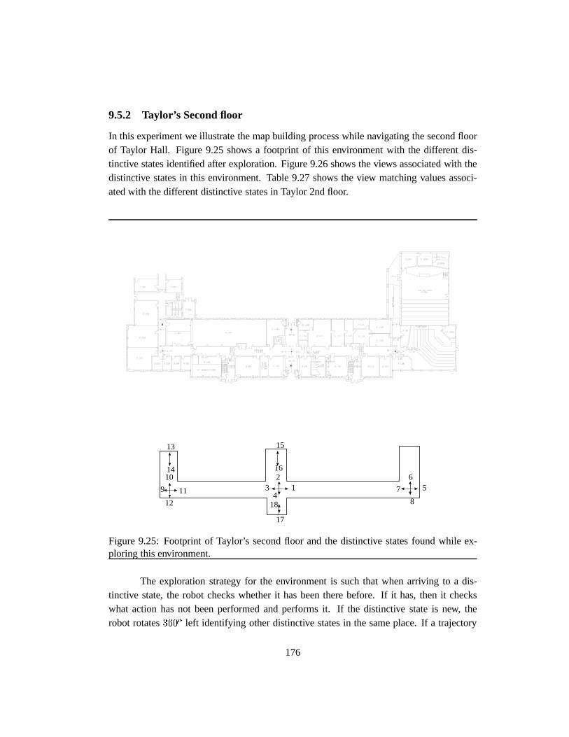
9.5.2 Taylor’s Second floor

In this experiment we illustrate the map building process while navigating the second floorof Taylor Hall. Figure 9.25 shows a footprint of this environment with the different dis-tinctive states identified after exploration. Figure 9.26 shows the views associated with thedistinctive states in this environment. Table 9.27 shows the view matching values associ-ated with the different distinctive states in Taylor 2nd floor.

8

510

15

16

17

12

34

18

6

7

13

14

9

12

11

Figure 9.25: Footprint of Taylor’s second floor and the distinctive states found while ex-ploring this environment.

The exploration strategy for the environment is such that when arriving to a dis-tinctive state, the robot checks whether it has been there before. If it has, then it checkswhat action has not been performed and performs it. If the distinctive state is new, therobot rotates360o left identifying other distinctive states in the same place. If a trajectory

176

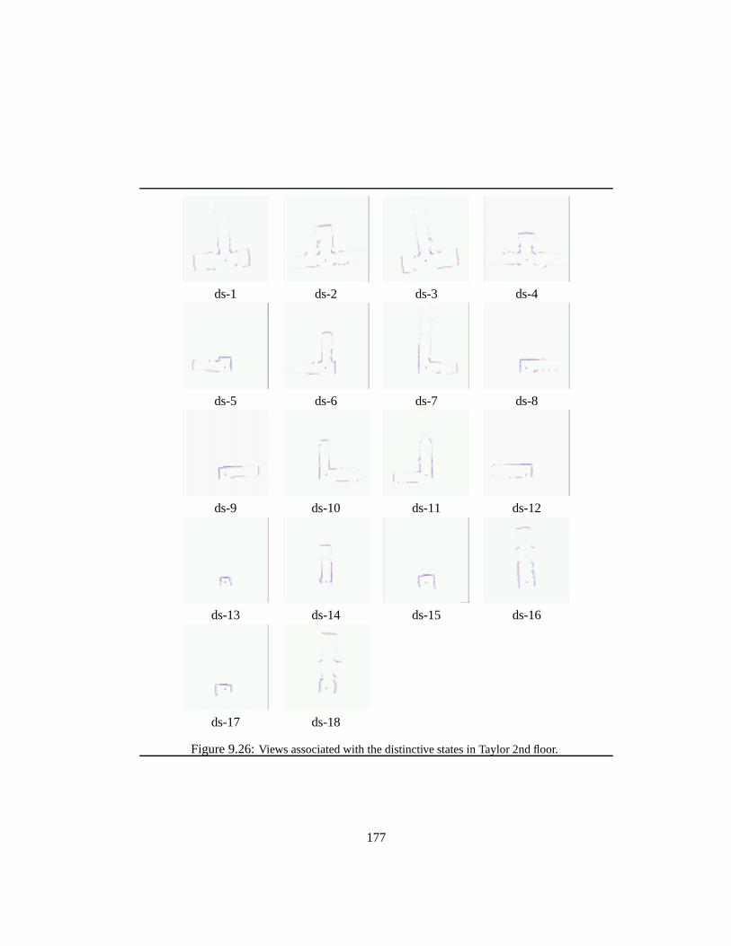
ds-1 ds-2 ds-3 ds-4

ds-5 ds-6 ds-7 ds-8

ds-9 ds-10 ds-11 ds-12

ds-13 ds-14 ds-15 ds-16

ds-17 ds-18

Figure 9.26:Views associated with the distinctive states in Taylor 2nd floor.

177

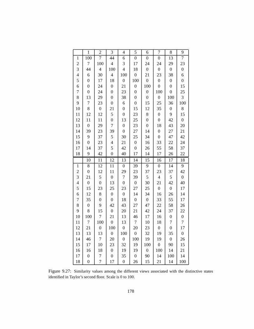
1 2 3 4 5 6 7 8 91 100 7 44 6 0 0 0 13 72 7 100 4 3 17 24 24 29 233 44 4 100 4 18 0 0 0 04 6 30 4 100 0 21 23 38 65 0 17 18 0 100 0 0 0 06 0 24 0 21 0 100 0 0 157 0 24 0 23 0 0 100 0 258 13 29 0 38 0 0 0 100 39 7 23 0 6 0 15 25 36 10010 8 0 21 0 15 12 35 0 811 12 12 5 0 23 8 0 9 1512 11 11 0 13 25 0 0 42 013 0 29 7 0 23 0 18 43 2014 39 23 39 0 27 14 0 27 2115 9 37 5 30 25 34 0 47 4216 0 23 4 21 0 16 33 22 2417 14 37 5 42 0 26 55 58 3718 9 42 0 40 17 14 17 26 22

10 11 12 13 14 15 16 17 181 8 12 11 0 39 9 0 14 92 0 12 11 29 23 37 23 37 423 21 5 0 7 39 5 4 5 04 0 0 13 0 0 30 21 42 405 15 23 25 23 27 25 0 0 176 12 8 0 0 14 34 16 26 147 35 0 0 18 0 0 33 55 178 0 9 42 43 27 47 22 58 269 8 15 0 20 21 42 24 37 2210 100 7 21 13 46 17 16 0 011 7 100 0 13 7 10 18 7 712 21 0 100 0 20 23 0 0 1713 13 13 0 100 0 32 19 35 014 46 7 20 0 100 19 19 0 2615 17 10 23 32 19 100 0 90 1516 16 18 0 19 19 0 100 14 2117 0 7 0 35 0 90 14 100 1418 0 7 17 0 26 15 21 14 100

Figure 9.27: Similarity values among the different views associated with the distinctive statesidentified in Taylor’s second floor. Scale is 0 to 100.

178

following strategy can be applied, the robot does so. Otherwise it rotates right to the clos-est distinctive state, where the procedure is repeated. Using this strategy the order in whichdistinctive states are visited for the environment of figure 9.25 is summarized in figure 9.28.

For the experiment we used a threshold value of0:6 in order to decide whether twolist of segments correspond to the same view. This value is consistent with the intraclasssimilarity value provided by our view matcher, as discussed in example 31 (page 140).Accordingly, in the Taylor second floor environment the robot experiences sensory aliasingfor distinctive states ds-15 and ds-17 (see figures 9.26 and 9.27). However, these distinctivestates are along the same path at different places, and topological information is enough todistinguish them (see figure 9.28).

179

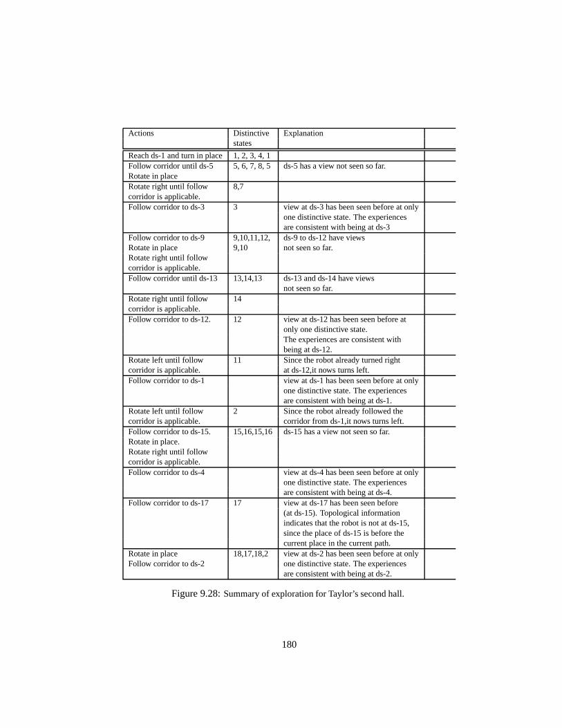
Actions Distinctive Explanationstates

Reach ds-1 and turn in place1, 2, 3, 4, 1Follow corridor until ds-5 5, 6, 7, 8, 5 ds-5 has a view not seen so far.Rotate in placeRotate right until follow 8,7corridor is applicable.Follow corridor to ds-3 3 view at ds-3 has been seen before at only

one distinctive state. The experiencesare consistent with being at ds-3

Follow corridor to ds-9 9,10,11,12, ds-9 to ds-12 have viewsRotate in place 9,10 not seen so far.Rotate right until followcorridor is applicable.Follow corridor until ds-13 13,14,13 ds-13 and ds-14 have views

not seen so far.Rotate right until follow 14corridor is applicable.Follow corridor to ds-12. 12 view at ds-12 has been seen before at

only one distinctive state.The experiences are consistent withbeing at ds-12.

Rotate left until follow 11 Since the robot already turned rightcorridor is applicable. at ds-12,it nows turns left.Follow corridor to ds-1 view at ds-1 has been seen before at only

one distinctive state. The experiencesare consistent with being at ds-1.

Rotate left until follow 2 Since the robot already followed thecorridor is applicable. corridor from ds-1,it nows turns left.Follow corridor to ds-15. 15,16,15,16 ds-15 has a view not seen so far.Rotate in place.Rotate right until followcorridor is applicable.Follow corridor to ds-4 view at ds-4 has been seen before at only

one distinctive state. The experiencesare consistent with being at ds-4.

Follow corridor to ds-17 17 view at ds-17 has been seen before(at ds-15). Topological informationindicates that the robot is not at ds-15,since the place of ds-15 is before thecurrent place in the current path.

Rotate in place 18,17,18,2 view at ds-2 has been seen before at onlyFollow corridor to ds-2 one distinctive state. The experiences

are consistent with being at ds-2.

Figure 9.28:Summary of exploration for Taylor’s second hall.

180

9.6 Summary

We have presented the main issues of a particular implementation of the SSH using Vulcan.At the SSH control level, an observer architecture is used to implement trajectory follow-ing and hill climbing control laws. The same control law (equation 9.1, page 130) used inconjunction with differentmodel trackers(figure 9.3, page 131) produces most of Vulcan’sbehaviors (for instance, follow a corridor, go through doorways, hill climb to a corridorintersection, etc.). The implementation satisfies the SSH control level guarantees: the robotbehaviors start and terminate in the neighborhood of the fixed points associated with hillclimbing strategies. While the focus of this dissertation has not been on the SSH controllevel, it is worthwhile noticing that in general implementing the control level in a physicalrobot is half of the battle when implementing the SSH.

Views at the causal level were defined in terms of segments extracted from a laserscan at the particular robot location (section 9.3, page 138). The results in example 31 andsection 9.5.2 (pages 142 and 178) show that this method is adequate in office like envi-ronments: the views there defined have a well defined discriminant boundary among thedifferent view classes identified by the robot. Our method uses one laser scan to define aview. Other methods exist where more than one laser scan (or multiple sensors) are used todefine a view ([Duckett and Nehmzow, 2000]). No attempt has been done to compare ourmethod to these other ones.

The implementation of the causal, topological and metrical levels has focussed onidentifying and keeping track of the different maps consistent with the agent’s experiences.A logic program derived from the circumscriptive theory defined in chapter 4 was definedfor calculating the causal models associated with a set of experiences (section 9.4.1, page147). The same technique unfortunately does not scale up when building the topologicalmap. The problem of building a topological map was stated then as a“best first” searchproblem. The states of the search correspond to partial models ofTT (E). At each stepof the search a schemah ds; a; ds0 i has to be explained. Either the identity ofds0 can beproved or a search branch is created for every previously known distinctive stateds00 that

cannot be proven to be different fromds0. In each branch the assumptionds00teq= ds0 will

be the case. The next state to explore is the one that is minimum according to the order as-sociated with the circumscription policy forTT (E). This search algorithm was describedin section 9.4.2 (page 152).

While not explicitly described in this chapter, the robot exploration strategy is such

181

that should more than one map be consistent with the robot experiences, the robot triesimmediately to distinguish among the different alternatives (i.e. the robot performs the re-hearsal procedure). The knowledge base is such that one could query for a sequence ofactions (and so observations) that will distinguish among the possible map alternatives.

Metrical information has been used torefutea given topological map by showingthat it is impossible to project the map into a two dimensional space preserving the esti-mated distance and relative orientation between consecutive places in a path (chapter 7,page 90). A more sophisticated use of metrical information has not been explored in theimplementation (for instance, occupancy models associated with a place has not been im-plemented). Sections 9.4.3 (page 161) and 9.5.1 (page 169) illustrate the use of metricalinformation while building the topological map.

182

Chapter 10

Related Work

In this section we review some of the relevant literature in the different areas comprisingthis work. These areas include: cognitive robotics, qualitative reasoning, robotics and mapbuilding.

10.1 Cognitive theories of space representation

Human knowledge of large-scale space is sometimes called thecognitive map.1 The cog-nitive map serves two functions with regard to wayfinding: representing environments, andthe corresponding ability to use the representation to move from place to place within themapped environment[Kortenkampet al., 1995]. Among the main characteristics of thecognitive map we have: the use of multiple frames of reference, qualitative representa-tion of metrical information, and connectivity relations among landmarks. Next we re-view the computational theories of the cognitive map that are closest to our current work.Some other systems can be found in[Leiser and Zilbershatz, 1989, Gopalet al., 1989,Gopal and Smith, 1990, O’Neill, 1991, Engelson and McDermott, 1992a, Yeap, 1988].

10.1.1 PLAN

Kortenkamp et al.[Kortenkampet al., 1995] have developed an integrated representationof large-scale space called PLAN (Prototypes, Location and Associative Networks). In this

1Large-scale space is defined as space whose structure is at a much larger scale than the sensory horizonof the agent. Thus, to learn a map, the agent must travel through the space, gathering local observations andinferring their global relationships from the actions linking them[Kuipers, 2000].

183

theory, landmarks function as a kind of environmental index. Recognizing nearby land-marks is enough to tell one where one is in a familiar environment. Objects (landmarks) arerepresented byprototypes.2 A network of landmarks is created as the agent travels the en-vironment. In this network, nodes represent landmarks and edges between nodes representthe agent’s ability to go between two proximate landmarks[J., 1991, Sch�olkopf and Mallot,1995]. Edges in the network have variable strength values associated with them.3

Directional space is represented by alocal map. A local map provides the relativechange in orientation for any neighboring target landmark. A local map is representedby a combination of a 2-D grid and a sectoring information with respect to a normalizedviewpoint.4 Local maps are created atgateways: places were a route choice point hadbeen reached and a new landmarks could be seen. A network of local maps is then createdassociated with the corresponding network of landmarks.

10.1.2 McDermott and Davis

McDermott and Davis have developed a theory where objects other than paths are repre-sented in the cognitive map[McDermott, 1980, McDermott and Davis, 1984, Davis, 1993].In addition to topological information, a “fuzzy map” is created for representing metricalinformation. A fuzzy map captures facts about objects by recording their relative positions,orientations, and scales in convenient frames of reference. Uncertainty in metrical informa-tion is represented by numerical intervals. Assimilation of new information might constrainthe uncertainty on metrical information. Hill climbing or Monte Carlo techniques are usedfor propagating metrical constraints[McDermott and Davis, 1984].

The MERCATOR program[Davis, 1993] constructs a cognitive map from a se-quence of scene descriptions. Objects are represented by sets of polygons. The relativepositions of objects are determined by connecting edges. The space representation accountsfor uncertainty on position and distance between objects, multiple shape description of thesame object, and representation of partial knowledge about objects spatial properties. Inaddition, operations on the map are justified by a formal semantics. In Appendix G wedescribe MERCATOR’s ontology as well as its associated semantics.

2Prototypes are generalizations derived from a range of experience. In such a generalization the featuresthat occur most often come to represent the prototype, whereas features that occur less often are weaker, givingthe prototype a statistical nature, reflecting experience[Kortenkampet al., 1995].

3Using fixed links to connect adjacent landmarks yields an inadequate model of human wayfinding. Familiarroutes are naturally easier to remember; routes that have only been traversed once or twice are going to bedifficult to re-create[Kortenkampet al., 1995].

4The representation of orientation information is similar to the one used by Hernandez[Hernandez, 1994].

184

10.2 Cognitive Robotics

The area of Cognitive Robotics studies the knowledge representation and reasoning prob-lems faced by an autonomous agent in a dynamic and incompletely known world. The goalis to develop an understanding of the relationship between the knowledge, the perception,and the action of such agent. With respect to robotics, the goal is ahigh level robotic con-trol: develop a system that is capable of generating actions in the world that are appropriateas a function of some current set of beliefs and desires. Most of the work in this area aimsfor a logical account for the sort of high level cognitive skills listed above. Robots whosedesign is based on logical representation have the virtue of producing behavior which can beaccounted for in terms ofcorrect reasoningandcorrect representation[Sandewall, 1996].Logics for reasoning about actions and planning are used in order to describe the actions ofthe robots as well as its environment[Shanahan, 1997b, Sandewall, 1994]. Formal specifi-cations are then used as a base to program robots[Lesperanceet al., 1994, Sandewall, 1997,Shanahan, 1998]. Next we summarize two of the main works in the area: the work done atthe University of Toronto (by Reiter and et al.) and the work done by Murray Shanahan.

10.2.1 GOLOG

The Cognitive Robotics project at the University of Toronto is concerned with endowingrobotic or software agents with higher level cognitive functions that involve reasoning, forexample, about goals, perception, actions, the mental states of other agents, collaborativetask execution, etc. To do this, they describe, in a language suitable for automated reason-ing (GOLOG), enough of the properties of the robot, its abilities, and its environment, topermit it to make high-level decisions about how to act. The situation calculus[McCarthyand Hayes, 1969] has been taken as the underlying language for reasoning about the pre-requisites and effects of actions, perception, knowledge-producing actions, natural eventsand actions by other agents[Reiter, 1996]. These methods have been incorporated into alogic programming language for agents called GOLOG (alGOl in LOGic).

GOLOG is a high-level programming language suitable for declaratively definingcomplex behaviors. In GOLOG[Lesperanceet al., 1994],

“The user provides a specification of the robot’s basic actions (their precon-ditions and effects on the environment) as well as of relevant aspects of the

185

environment, in an extended version of the situation calculus. He can thenspecify robot behaviors in terms of these actions in a programming languagethat allows references to world conditions (e.g.if 9c(pop can(c)^on table(c))

then pick up(c)). The programs can be executed to drive the robot. The inter-preter automatically maintains the world model required to execute programsbased on the specification. The theoretical framework includes a solution tothe frame problem and is very general (it handles dynmaic and incompletelyknown worlds, as well as perception actions). Given this kind of domain spec-ification, it is also possible to support more sophisticated reasoning, such astask planning at run-time. The specification can also be used to prove the robotcontrol programs correct”.

Recently, GOLOG has been extended to CONGOLOG (CONcurrent GOLOG)[De Gi-acomoet al., 1997] which includes facilities for concurrent execution, interrupting the exe-cution when certain conditions become true, and dealing with exogenous actions.

10.2.2 Shanahan’s Work

Shanahan[Shanahan, 1996, Shanahan, 1997a] proposes a logic-based framework in whicha robot constructs a model of the world through an abductive process whereby sensor datais explained by hypothesising the existence, locations, and shapes of objects. In[Shanahan,1998] this work is augmented by an account forplanningas well as an implementation ofthese ideas via an abductive logic programming metainterpreter. Next we summarize themain points of these formalizations.

Given a stream of sensor data, represented as the conjunction� of a set of observationsentences, the task is to find an explanation of� in the form of a logical description (amap)�M of the initial locations and shapes of a number of objects, such that,

KB ^�M j= �

whereKB is a theory comprising axioms for change, action, space, relations betweenmovements of objects and robot’s sensor data, the movements executed by the robot, etc.5

Thesemanticsof an agent’s space representation,M , is a formula,�(M), in the languageof KB, such that�(M) postulates the initial locations and shapes of a number of objects.As an agent travels through its environment, it executes a set of actions,A, and experiences

5KB is expressed in the circumpscritive event calculus[Shanahan, 1997b].

186

a set of observations�. As a result, the agent constructs its own space representation,M .We defineM to becorrect with respect to (A,�) if

KB ^A ^�(M) j= �

Note thatA and� are expressed in the language ofKB whileM is expresed in the agent’slanguage.

Shanahan’s space formalization only asks for the locations and shapes of objects. In Shana-han’s work, space is considered a real-valued coordinate system6, shape is represented as acollection of straight lines, and the set of agent’s actions isfgo,stop,rotate(r)g. KB is basedon these choices to represent space, shape and actions. It does not specify what the behaviorof the agent should be: it specifies what space information can be derived from the actualbehaviour and observations of the agent.

Planning can be thought of as the inverse operation to temporal projection, andtemporal projection in the event calculus is naturally cast as a deductive task. Consequently,planning in the event calculus can be considered as an abductive task. Given a domaindescription�, a conjunction� of goals, and a description of the initial situation,�N , aplan is a consistent conjuction�p of Happensand a temporal ordering formulae such that

� ^�N ^�p j= �:

This logical characterization of the event calculus planning is analgous to Green’s logicalcharacterization of situational calculus planning[Green, 1969].

10.3 Qualitative Representation of Space

Qualnav model [Kuipers and Levitt, 1988, Levitt and Lawton, 1990]. The Qualnavmodel provides a computable theory that integrates qualitative, topological representationsof large-scale space with quantitative, metric ones. A difference from the TOUR model,Qualnav considers unstructured environments, with significant perceptual events, calledlandmarks, scattered throughout this two-dimensional space.

Qualitative navigation is carried out by identifiyinglandmark-pair boundaries(LPBs)between landmarks. Roughly speaking, a LPB between landmarksL1 andL2 is a virtualline betweenL1 andL2. This line divides the space into two distinct regions. If the agent

6He does not rule out the adoption of qualitative approaches to spatial reasoning.

187

can observe the landmarks, it can decide then which side of this line it is on. LPBs give riseto a topological division of the ground surface into observable regions of localization,theorientation regions. Crossing boundaries between orientation regions leads to a qualitativesense of path planning based on perceptual information. As a landmark-recognizing visionsystem moves through large-scale space, it builds a visual memory of the interlocking se-quence of orientation regions it has traversed through. Adjacency of orientation regions invisual memory can be determined by sharing a common but opposite orientation LPB. Iftwo regions have a common boundary, it is possible to move between them by tracking thelandmarks as the agent moves towards the boundary. Thus,visual memory is an undirectedgraph where nodes are orientation regions, and arcs join adjacent regions.

Hernandez[Hernandez, 1994] provides a model for the qualitative representationof positional information in 2-D space based on topological and orientation relations. Us-ing Freska’s notion ofconceptual neighborhood for qualitative relations[Freksa, 1992],algorithms for transforming between explicit reference frames and a canonical one, as wellas for composing spatial relations are defined. In addition,[Hernandez, 1994] presents avariety of mechanisms to reason with qualitative representations in general, and qualitativerepresentations of 2-D positional information in particular. These mechanisms are based onthe idea of modifying domain independentconstraint satisfactiontechniques to account forthe particular constraints of the spatial domain. Moreover, special data structures are usedfor improving the efficiency of the algorithms. In particular,abstract maps, are introduced,containing for each object in a scene a data structure with the same neighborhood structureas the domain requires for the task at hand. A change of view, for example, can then easilyaccomplished diagrammatically by “rotating” the labels of the orientation with respect tothe intrinsic one.

Hernandez[Hernandez, 1994] presents an extensive review of the different ap-proaches to the representation of spatial knowledge (see chapter eight). The integrationof metric and path knowledge with qualitative representations of space is not covered inthis work. As for path knowledge, Hernandez states that

“the positional information implicitly contained in paths can be gradually as-similated in form of topological and orientation relations by a process in whichpositional relations are established for the (virtual) places at which directionalchange occur. The positions of the actual objects in the scene are then derivedby constraint propagation”.

188

10.4 Robotics

Two main areas of robotics are primarily related to our work: map building and autonomousnavigation. The map building problem refers as to how the robot creates a spatial represen-tation of its enviroment. Two common spatial representations are geometric and topologicalmaps. A geometric map represents objects according to their absolute geometric relation-ships (more later). In contrast, a topological map records the geometric relationships be-tween the observed features rather than their absolute position with respect to an arbitrarycoordinate frame of reference (see 10.1). The problem of robot navigation corresponds toreliably go from one place to another in the environment. During the navigation, the robotuses its sensors to create a map of its local environment. This local map is then compared toa global spatial representation in order to calculate its position in the environment. We areinterested in how the spatial representation supports the “sense-plan-act” navigation cycle.Next we review some of the work we have borrowed ideas from. We refer the reader toKortenkamp et al.’s book[Kortenkampet al., 1998] for an extensive review of AI mobilerobot systems and techniques.

10.4.1 Metrical maps

The most common representation of geometric map data is acertainty grid [Elfes, 1987,Borestein and Koren, 1991]. In a certainty grid approach, sensor readings are placed into thegrid by using probability profiles that describe the algorithm’s certainty about the existenceof objects at individual grid cell. When positioning with respect to a metrical map, sensorderived geometric maps must be matched against a global map of a large area. This is oftena formidable difficulty because of the robot’s position error. Using topological informationhas proven be useful in order to reduce the effect of position error when constructing ametrical map[Thrun, 1998, Thrunet al., 1998]. We refer the reader to Borestein’s book[Borensteinet al., 1996] (Chapter 8) for a review of the problems and advantages usingmetrical maps as well as a description of several systems using this spatial representation.

10.4.2 Fuzzy control

Konolige et al. [Konolige et al., 1995] propose an approach for integrating planning andcontrol based onbehavior schemas, which link physical movements to abstract action de-scriptions. Behavior schemas describe behaviors of an agent, expressed as trajectories ofcontrol actions in an environment, and goals can be defined as predicates on these trajecto-ries. The proposed methodology is summarized as follows[Konoligeet al., 1995]:

189

“Our approach to integrating planning and control has focussed on groundingthe ingredients of planning in physical actions, using the tools of multivaluedlogics. We started from the definition of basic types of movements, orcontrolschemas, and of the way they can be combined or blended to form complexbehaviors. Then we have “lifted” control schemas to the level of abstract ac-tions in the environment. Here, we have used two key notions: the notion ofembeddingin the environment, by anchoring the agent’s internal state to ex-ternal objects through perception, and the notion ofcontext, or circumstancesof execution. Finally, we have linked behaviors to goals, expressed as sets ofsatisfactory executions. The good behaviors for a goal are those that, when ex-ecuted in the appropriate context, produce executions that satisfy the goal. Andwe have proven, under certain hypotheses, that composing behaviors creates anew behavior that is good for the composition of the corresponding goals. Thisresult is the basis for automatic planning of complex behavior, and we haveshown how traditional AI techniques for deliberation and means-ends analysiscan be readily adapted to generate complex controllers for given goals”.

10.4.3 Probabilistic navigation

In probabilistic navigation, the location of a robot is represented by a probability distri-bution over the possible locations of the robot. The robot’s position is updated based onthe actions it executed as well as observations gathered during navigation. The methodtakes into account various sources of uncertainty, including approximate knowledge of theenvironment, and actuator and sensor uncertainty[Simmons and Koening, 1995, Koeningand Simmons, 1998, Nourbakhsh, 1998]. A partially observable Markov decision process(POMDP)7 model is constructed from topological information about the connectivity of theenvironment, approximate distance information, plus sensor and actuator characteristics.

7See section A.1.2, page 203.

190

Chapter 11

Conclusions and Future Work

What have we done?. We have taken an informal description of the SSH[Kuipers and Byun,1988, Kuipers and Byun, 1991, Kuipers, 2000] and given a formal account of some aspectsof this theory. In addition, we have extended the theory to handle perceptual aliasing, envi-ronments with self intersecting and convergent paths, as well as to deal with local metricalinformation uncertainty. The new description of the SSH is independent of the agent’s ex-ploration strategy and the possible implementations of the theory. This in contrast to theprevious SSH descriptions as well as applications of topological maps in robotics[Chosetand Nagatani, 2001]. Nevertheless, we have taken the new SSH description as a specifi-cation for a program able to keep track of different topological maps consistent with theagent’s experiences in the environment. This program supports different exploration strate-gies as well as facilitating map disambiguation when the case arises.

A logical account of the SSH causal, topological and local metrical theories wasgiven using Nested Abnormality theories[Lifschitz, 1995]. The minimality conditions em-bedded in the formalization defined the preferred models associated with the theories. Inchapters 4 through 8 we illustrated the main properties of the new theories. In particular weshowed how the minimal models associated with these theories are adequate models for thespatial knowledge an agent has about its environment. We also illustrated how the differentlevels of the representation assume different spatial properties about both the environmentand the actions performed by the agent. These spatial properties play the role of “filters”the agent applies in order to distinguish the different environment states it has visited.

In the process of formalizing the SSH we have improved the theory in the followingaspects:

� Extended the SSH ontologies to include distinctive states, explicitly mention actions

191

at the topological level, and deal with local metrical information uncertainty.

� Handled perceptual aliasing.

� Associated a spatial representation with the SSH causal level.

� Defined the models of the SSH causal and topological theories.

� Added a theory of regions.

� Extended the topological theory to handle environments with convergent and selfintersecting paths.

Distinctive states have been included as explicit objects in the theory. The predi-catesceq andteq (chapters 4 and 5) were introduced to denote when two distinctive statesare equal given causal and topological information, respectively. Local metrical informa-tion imposes further constraints on distinctive states (chapter 7). Having distinctive statesas objects allows the theory to deal with perceptual aliasing (i.e. environment states thatlook the same). Once perceptual aliasing is introduced, more than one model of the theorycould explain a given set of experiences. In such cases, new information could prove envi-ronment states to be different although they were previously believed equal, and viceversa.Our theory captures this non-monotonicity property of map building.

At the SSH causal level we introduced a spatial representation, that of the causalgraph. A causal graph is a deterministic finite automaton (DFA) where states areceq equiv-alence classes. Actions at the causal level convey patterns of experience, but no spatialconfiguration. At the SSH topological level, qualitative spatial information in terms ofturnandtravel actions is explained in terms of places, paths and regions. Local metrical infor-mation associated with action execution is explained in terms of distance among places on apath and angle among paths that intersect at a place. While the ontology of the topologicaland metrical levels is more elaborated than the one for the causal level, it is easier to buildthis representation than it is to distinguish environment states based only on view-action-view sequences.

We studied the appropriateness as well as the limitations of the theory. In particular,we illustrated how when sensor information is weak or the environment is symmetric, theSSH topological map may not have the same structure as the “real environment”. In suchcases, the topological map has fewer places and paths than the ones one would expect (seepage 24). Nevertheless, the model is sound in that any view-action-view sequence it pre-dicts will indeed be attainable in the environment.

192

From a pragmatical point of view, we illustrated how different navigation architec-tures are supported by the SSH (appendix A) and we tested these architectures in simulationand the physical robot Vulcan (chapter 9). Although for map building purposes actions areconsidered deterministic, during navigation errors in action execution occur. We defineddifferent approaches that the SSH can accommodate in order to deal with errors in actionexecutions and location uncertainty. Similarly, we defined how the SSH representation canbe used for planning, in particular, how regions support hierarchical planning and execution.

In summary, we have defined the SSH models associated with a set of experi-ences. The resulting theory exhibits some of the agent’s map building characteristics: non-monotonicity, use of different sources of information, multiple models when using weaksensors or when the environment is symmetric. The theory’s implementation supports dif-ferent robot exploration strategies and navigation strategies. It is our aim, that this theory aswell as the algorithms proposed will constitute the standard for map building applicationsbased on topological maps.

11.1 Future work

There are several different areas of future research linked to this work. These areas include:extensions of the theory, dealing with non-structured (open) environments, and reasoningwith multiple spatial representations. We discuss these areas in turn.

11.1.1 Extension for the current theory

Our theory assumes static environments. This assumption is embedded in two axioms: ac-tions are deterministic and distinctive states have a unique view. The first axiom relies onthe control level satisfying the SSH closure properties. The second axiom relies on theagent having perceptual recognition abilities such that the same view is associated with anyenvironment state “close enough” to a given distinctive state. However, actions could fail(i.e. miss a distinctive state) and environment states could have different views associatedwith then (e.g. a door being closed or opened). How should the theory be extended to dealwith non-static environments?. Should probabilistic modeling be used instead of the currentlogical approach?.

A major point of the SSH theory is that the topological map can be built even inthe presence of no metrical information. Nevertheless, whenever the agent decides to cre-ate a region and assign locations to places in that region, path shapes should be taken into

193

account. How should a path’s shape be represented and reasoned about?. Are qualitativedescription of path shape enough?

11.1.2 Learning the control level

While the SSH control level implementation was not the focus of this dissertation, manyinteresting questions need to be solved to carry on such implementation. First at all, onehas to translate sensory input into views. Views are then seen as classes describing sensoryinput. How does a robot learns these classes? How many classes should it learn?. Second,the agent control laws are predefined. Different representations of the same environmentresult from using different sets of views and control laws. How does the agent decides whatset of control laws are appropriate for exploring the environment?1. Third, the control levelhas to render actions deterministic. While we rely on control theory to satisfy this require-ment, learning control law parameters could benefit from machine learning techniques. Inparticular, as the agent repeatedly explores the environment, one expects a more reliableexecution of control laws.

11.1.3 Open environments

We have tested the SSH in office-like environments and simulation. What does it take tohave a SSH robot navigating non-structured open environment, say a university campus?or a museum? Will the current theory be useful? How much does one have to engineer thecontrol level to define the “right” set of actions to handle each environment? Certainly beingable to learn the control level (as stated above) will greatly simplify the task of exploringthese environment. We also anticipate that the use of different topological hierarchies (see11.1.4) as well as the representation of local space will be important for these tasks.

In order to engineer a SSH robot, local representations of space should be incor-porated. For example, it is easier to navigate a cluttered room based on a reactive visionmodule or an occupancy metrical representation, than it is in terms of control laws mov-ing the robot between distinctive states. Techniques to do this navigation exists, and theSSH incorporates these local space representations, but the question remains of when thesechanges of representation occur, and how the agent keeps the relations among these repre-sentations.

1See 11.1.4 below.

194

11.1.4 Reasoning with multiple spatial representations

The SSH is a hierarchy of coexisting spatial representations. At the same time, the SSHtopological level admits a hierarchical representation based on regions. There are otherkind of topological hierarchies based on scale granularity or relations among actions. Theseapproaches admit building more detailed maps based on a existing map. For instance,the agent first builds the map using a general control law (likefollow-corridor) which isthen refined when executing a particular instance of such control law (likefollow-corridor-stopping-at-doorways). From the relation among the actions, one could relate both repre-sentations. The question remains of how/why an agent builds such hierarchies, how theyare related, and how/when an agent uses them for spatial reasoning?

195

Appendix A

Using the SSH

The appropriateness of the SSH representation derives from how well it supports large scalenavigation. Navigation is understood here as the task of getting from one place to another.This process involves three main aspects: localization, planning, and plan execution. Lo-calization is the process of knowing the current location of the agent in the environment.Planning is determining the actions that should be executed to get to the destination place,and plan execution is the process of carrying out these actions.

Different architectures exist for implementing robot navigation. The major goal ofthese architectures is to show how the agent reaches its destination place despite errors inaction execution as well as noise in sensory input. They vary on how the cycle of local-ization, planning and plan execution is carried out, as well as on the kind of informationthe spatial representation should provide for their success. In this chapter we show howthe SSH is suitable as the spatial representation for different navigation architectures.Ourgoal is to show how the spatial representation (the SSH) is used by different existingnavigation architectures rather than to define “the” SSH navigation architecture.

This chapter is organized as follows. Section A.1 illustrates how uncertainty aboutthe agent’s location can be represented in the context of the SSH. In section A.2 we showhow SSH topological paths and regions are used when planning a route to a goal location.Different navigation architectures supported by the SSH are presented in section A.3.

A.1 Location

The locationof the agent in the environment is described in terms of theregion, place, andthepath the agent is at.We assume that a map of the environment is given to the agent.

196

The agent may not know its actual location w.r.t. this map as actions may fail or viewsare not enough to discern the location. Consequently, the agent has to represent the uncer-tainty associated with its current location and act according to it. Next we will present twodifferent representations of uncertainty that can be accommodated when using the SSH: inthe first one, a set of locations represents the possible locations the agent is at; in the sec-ond representation, a probability distribution is kept over the universe of locations. In bothcases, one has to provide astate transition functiondefining the effect of actions when exe-cuted at particular states (locations), as well as to provide anobservation modeldescribingthe effect of making a particular observation at a particular state.

A.1.1 Representing location knowledge

Suppose the agent’s current location is represented by a set of locations (states),�, theagent believes it may be at. Under this representation, given an actiona, one has to specifythe effect ofa on�, which we will denote by�a. By definition,

�a =�s0 : 9s 2 � ; h s; a; s0 i

(A.1)

whereh s; a; s0 i denotes the fact that states0 is a possible result of executing actiona onstates. The tuplesh s0; a; s0 i define the possible state transitions associated with the agentactions. Different languages can be used to specify these transitions. For example, STRIPS([Fikes and Nilsson, 1971]), AC ([Baral and Gelfond, 1997]), C ([Giunchiglia and Lifs-chitz, 1998]).1

Definition A.1 is akin to the one given by Bacchus, Halpern and Levesque in thecontext of reasoning about knowledge in the situation calculus ([Bacchuset al., 1999], page182). They in turn draw in Moore’s work[Moore, 1979, Moore, 1985] on usingpossibleworld semanticsto formally reason about knowledge and actions. Here we have adaptedtheir definition in the context of transition based approaches to reason about actions ([Gel-fond and Lifschitz, 1998, Son and Baral, 2001, Loboet al., 1997]). Example 35 (page 200)illustrates how definition A.1 works. In particular, we will show how as the agent executesactions and makes observations, the set� captures the agent’sknowledgeabout its actuallocation. A formal study of how the knowledge of the agent changes as it performs actionsis outside the scope of this work. The reader is referred to[Moore, 1979, Moore, 1985,Scherl and Levesque, 1993, Bacchuset al., 1999, Son and Baral, 2001] for formal accountsof how to reason about actions and knowledge.

1We will useC to illustrate the concepts presented in this section.

197

We use the languageC ([Giunchiglia and Lifschitz, 1998]) to describe the effectof actions on the agent’s location. The fluentloc(p,pa,dir) is used to represent thatthe agent is atplace pfacing directiondir of path pa.2 Constraints between the differentelements describing a location can be derived from the SSH topological axioms (see chapter5). For example, if the agent is at placep on pathpa, it should be the case thatp belongs topathpa (i.e. on(pa; p) is true). The topological map is described in terms of the followingpredicates (see chapters 5,6,8):

� on(pa,p) : placep is on pathpa.

� order(pa,dir,p,q) : placeq is after placep on directiondir of pathpa.

� nextPlace(pa,dir,p,q) : placeq is the next place after placep on pathpa.

� viewsAt(p,v) : v is a view occurring at placep.

� totheRightOf(p,pa,dir,pa1,dir1), totheLeftOf(p,pa,dir,pa1,dir1)

: if the agent is placep facing on directiondir of pathpa, after executing a turn right(left) action, the agent will be facing on directiondir1 of pathpa1.

Views at the SSH causal level (chapter 4) are associated with places and used asevidence for the agent to be at a given place. We use the predicateviewsAt(p,v) torepresent that viewv occurs at placep. Whether a view occurs at a place can be determinedfrom the distinctive states associated with the place. Formally,

viewsAt(p; v) � 9ds fat(ds; p) ^ view(ds; v)g :

In addition to moving in the environment the agent cansensethe environment and deter-mine the view at its current location. The transitions needed by equation A.1 are describedby the following theory:3

Notice that we assume actions to be deterministic during map building, and explic-itly model action errors during navigation. Think of this as somebody giving you a map ofa city, and you using it for navigation. While visiting the city, you might get lost or missan intersection. You use the map as a reference to deduce where you may be at given thatthese errors occurred.Errors in travel actionsare modeled by considering a travel action asa non-deterministic action, whose effect is to move the agent along the same path but to a

2In this presentation we do not include regions in the agent’s location.3The theory is expressed in the languageC [Giunchiglia and Lifschitz, 1998] augmented with sorts as

recognized by Ccalc[McCain, 1999].

198

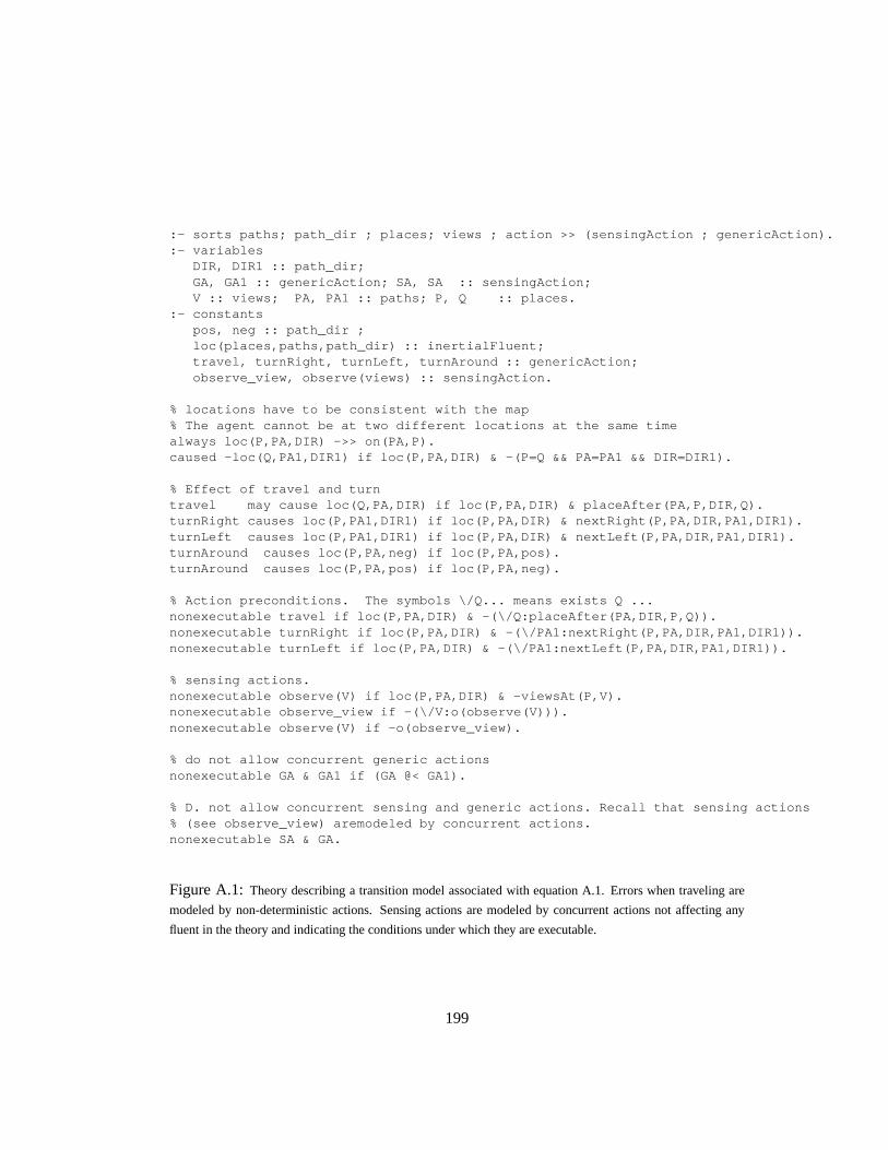
:- sorts paths; path_dir ; places; views ; action >> (sensingAction ; genericAction).:- variables

DIR, DIR1 :: path_dir;GA, GA1 :: genericAction; SA, SA :: sensingAction;V :: views; PA, PA1 :: paths; P, Q :: places.

:- constantspos, neg :: path_dir ;loc(places,paths,path_dir) :: inertialFluent;travel, turnRight, turnLeft, turnAround :: genericAction;observe_view, observe(views) :: sensingAction.

% locations have to be consistent with the map% The agent cannot be at two different locations at the same timealways loc(P,PA,DIR) ->> on(PA,P).caused -loc(Q,PA1,DIR1) if loc(P,PA,DIR) & -(P=Q && PA=PA1 && DIR=DIR1).

% Effect of travel and turntravel may cause loc(Q,PA,DIR) if loc(P,PA,DIR) & placeAfter(PA,P,DIR,Q).turnRight causes loc(P,PA1,DIR1) if loc(P,PA,DIR) & nextRight(P,PA,DIR,PA1,DIR1).turnLeft causes loc(P,PA1,DIR1) if loc(P,PA,DIR) & nextLeft(P,PA,DIR,PA1,DIR1).turnAround causes loc(P,PA,neg) if loc(P,PA,pos).turnAround causes loc(P,PA,pos) if loc(P,PA,neg).

% Action preconditions. The symbols \/Q... means exists Q ...nonexecutable travel if loc(P,PA,DIR) & -(\/Q:placeAfter(PA,DIR,P,Q)).nonexecutable turnRight if loc(P,PA,DIR) & -(\/PA1:nextRight(P,PA,DIR,PA1,DIR1)).nonexecutable turnLeft if loc(P,PA,DIR) & -(\/PA1:nextLeft(P,PA,DIR,PA1,DIR1)).

% sensing actions.nonexecutable observe(V) if loc(P,PA,DIR) & -viewsAt(P,V).nonexecutable observe_view if -(\/V:o(observe(V))).nonexecutable observe(V) if -o(observe_view).

% do not allow concurrent generic actionsnonexecutable GA & GA1 if (GA @< GA1).

% D. not allow concurrent sensing and generic actions. Recall that sensing actions% (see observe_view) aremodeled by concurrent actions.nonexecutable SA & GA.

Figure A.1: Theory describing a transition model associated with equation A.1. Errors when traveling are

modeled by non-deterministic actions. Sensing actions are modeled by concurrent actions not affecting any

fluent in the theory and indicating the conditions under which they are executable.

199

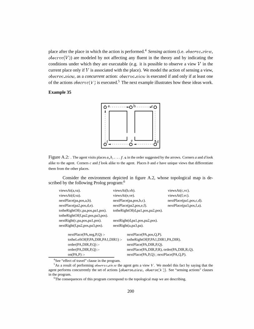
place after the place in which the action is performed.4 Sensing actions(i.e. observe view,observe(V )) are modeled by not affecting any fluent in the theory and by indicating theconditions under which they are executable (e.g. it is possible to observe a viewV in thecurrent place only ifV is associated with the place). We model the action of sensing a view,observe view, as aconcurrentaction:observe view is executed if and only if at least oneof the actionsobserve(V ) is executed.5 The next example illustrates how these ideas work.

Example 35

d

a

f e

b c

Figure A.2:. The agent visits placesa; b; : : : ; f; a in the order suggested by the arrows. Cornersa andd look

alike to the agent. Cornersc andf look alike to the agent. Placesb ande have unique views that differentiate

them from the other places.

Consider the environment depicted in figure A.2, whose topological map is de-scribed by the following Prolog program:6

viewsAt(a,va). viewsAt(b,vb). viewsAt(c,vc).viewsAt(d,va). viewsAt(e,ve). viewsAt(f,vc).nextPlace(pa,pos,a,b). nextPlace(pa,pos,b,c). nextPlace(pa1,pos,c,d).nextPlace(pa2,pos,d,e). nextPlace(pa2,pos,e,f). nextPlace(pa3,pos,f,a).totheRightOf(c,pa,pos,pa1,pos). totheRightOf(d,pa1,pos,pa2,pos).totheRightOf(f,pa2,pos,pa3,pos).nextRight(c,pa,pos,pa1,pos). nextRight(d,pa1,pos,pa2,pos).nextRight(f,pa2,pos,pa3,pos). nextRight(a,pa3,pa).

nextPlace(PA,neg,P,Q) :- nextPlace(PA,pos,Q,P).totheLeftOf(P,PA,DIR,PA1,DIR1) :- totheRightOf(P,PA1,DIR1,PA,DIR).order(PA,DIR,P,Q) :- nextPlace(PA,DIR,P,Q).order(PA,DIR,P,Q) :- nextPlace(PA,DIR,P,R), order(PA,DIR,R,Q).on(PA,P) :- nextPlace(PA,P,Q) ; nextPlace(PA,Q,P).

4See “effect of travel” clause in the program.5As a result of performingobserve view the agent gets a viewV . We model this fact by saying that the

agent performs concurrently the set of actionsfobserve view; observe(V )g. See “sensing actions” clausesin the program.

6The consequences of this program correspond to the topological map we are describing.

200

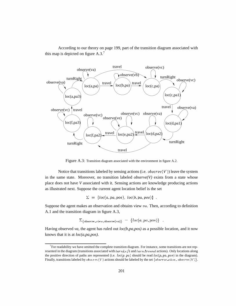
According to our theory on page 199, part of the transition diagram associated withthis map is depicted on figure A.3.7

observe(vc)

observe(va)travel observe(vc)

turnRightobserve(vc)

observe(vb)

traveltravel

travel

travel

turnRight

travel

travel loc(d,pa2)loc(e,pa2)loc(f,pa2)

loc(f,pa3)

loc(a,pa3)

loc(b,pa) loc(c,pa)

loc(c,pa1)

loc(d,pa1)

travel

turnRight

observe(vc)observe(ve)

observe(vc) observe(va)

observe(va)

observe(va)turnRight

loc(a,pa)

Figure A.3:Transition diagram associated with the environment in figure A.2.

Notice that transitions labeled by sensing actions (i.e.observe(V )) leave the systemin the same state. Moreover, no transition labeledobserve(V)exists from a state whoseplace does not haveV associated with it. Sensing actions are knowledge producing actionsas illustrated next. Suppose the current agent location belief is the set

� = floc(a; pa; pos); loc(b; pa; pos)g :

Suppose the agent makes an observation and obtains viewva. Then, according to definitionA.1 and the transition diagram in figure A.3,

�fobserve view;observe(va)g = floc(a; pa; pos)g :

Having observedva, the agent has ruled outloc(b,pa,pos)as a possible location, and it nowknows that it is atloc(a,pa,pos).

7For readability we have omitted the complete transition diagram. For instance, some transitions are not rep-resented in the diagram (transitions associated withturnLeft andturnAround actions). Only locations alongthe positive direction of paths are represented (i.e.loc(p; pa) should be readloc(p; pa; pos) in the diagram).Finally, transitions labeled byobserve(V ) actions should be labeled by the setfobserve view; observe(V )g.

201

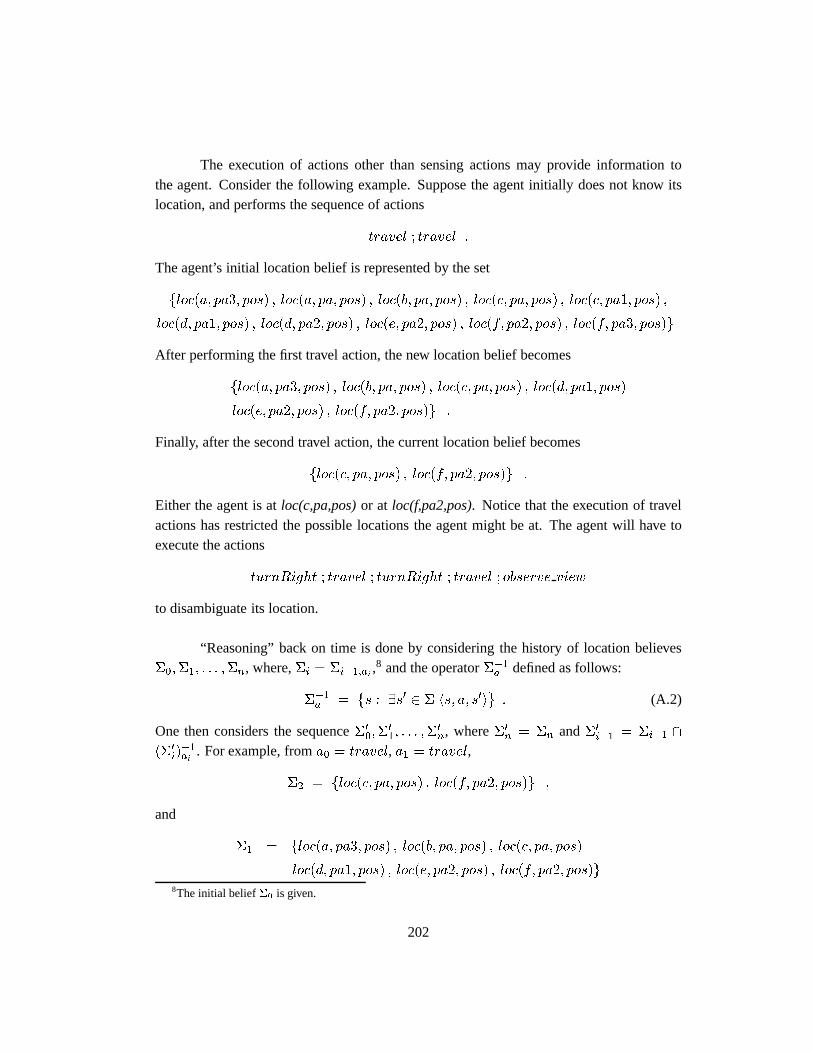
The execution of actions other than sensing actions may provide information tothe agent. Consider the following example. Suppose the agent initially does not know itslocation, and performs the sequence of actions

travel ; travel :

The agent’s initial location belief is represented by the set

floc(a; pa3; pos) ; loc(a; pa; pos) ; loc(b; pa; pos) ; loc(c; pa; pos) ; loc(c; pa1; pos) ;

loc(d; pa1; pos) ; loc(d; pa2; pos) ; loc(e; pa2; pos) ; loc(f; pa2; pos) ; loc(f; pa3; pos)g

After performing the first travel action, the new location belief becomes

floc(a; pa3; pos) ; loc(b; pa; pos) ; loc(c; pa; pos) ; loc(d; pa1; pos)

loc(e; pa2; pos) ; loc(f; pa2; pos)g :

Finally, after the second travel action, the current location belief becomes

floc(c; pa; pos) ; loc(f; pa2; pos)g :

Either the agent is atloc(c,pa,pos)or at loc(f,pa2,pos). Notice that the execution of travelactions has restricted the possible locations the agent might be at. The agent will have toexecute the actions

turnRight ; travel ; turnRight ; travel ; observe view

to disambiguate its location.

“Reasoning” back on time is done by considering the history of location believes�0;�1; : : : ;�n, where,�i = �i�1;ai ,

8 and the operator��1a defined as follows:

��1a =�s : 9s0 2 � hs; a; s0i

: (A.2)

One then considers the sequence�00;�01; : : : ;�

0n, where�0n = �n and�0i�1 = �i�1 \

(�0i)�1ai

. For example, froma0 = travel, a1 = travel,

�2 = floc(c; pa; pos) ; loc(f; pa2; pos)g ;

and

�1 = floc(a; pa3; pos) ; loc(b; pa; pos) ; loc(c; pa; pos)

loc(d; pa1; pos) ; loc(e; pa2; pos) ; loc(f; pa2; pos)g8The initial belief�0 is given.

202

as above, we conclude

�01 = floc(b; pa; pos) ; loc(e; pa2; pos)g :

By a further application of equation A.2 the agent concludes that its initial location beforeexecutingtravel; travel was eitherloc(a,pa,pos)or loc(d,pa2,pos).fend of exampleg

A.1.2 Probabilistic representations of location

Under the probabilistic approach to representing location uncertainty, a probability distri-bution is kept over the universe of locations. Transition and observation models have to beprovided defining the effect of actions on the different states. Based on these models, a rulehas to be defined on how to update the probability distribution after an action is executed.Next we illustrate the use of POMDP9 in the context of the SSH. The reader is referred to[Shafer, 1976, Duboi and Prade, 1988, Bacchuset al., 1999] for other possible approaches.

A POMDP is a tuple (S,A,T,�,O) 10 where:S is a finite set of states,A is a finiteset of actions,T is a state transition modelof the environment, which is a function mappingelements from SxA into discrete probability distributions over S,� is a finite set of possi-ble observations, andO is an observation function mapping AxS into discrete probabilitydistributions over�.

We writeP (s0ja; s) for the probability that the environment will make a transitionfrom states to states0 when actiona is executed. By definitionP (s0ja; s) = T (s; a; s0).We writeP (oja; s) for the probability of making observationo after having executed actiona and ended in states. By definition,P (oja; s) = O(a; s; o).

According to Bayes rule, given a current distributionPprior, an actiona, and an ob-servationo, we can calculate the distribution after performinga and observingo , Pposterior,as follows:

Pposterior(s0) = Pr(s0ja; o; Pprior) (A.3)

9POMDP stands for Partially Observable Markov Decision Process.10A POMDP includes also a reward function mapping SxA to the real numbers that specify the instantaneous

reward that the agent derives from taking an action in a state (see[Puterman, 1994]).

203

=Pr(ojs0; a; Pprior)Pr(s

0ja; Pprior)

Pr(oja; Pprior)

=P (oja; s0)

Ps2S P (s

0ja; s)Pprior(s)

Pr(oja; Pprior)

wherePr(oja; Pprior) is a normalizing factor defined as

Pr(oja; Pprior) =Xs02S

P (oja; s0)Xs2S

P (s0ja; s)Pprior(s) :

Example 36

Consider the same environment as in example 35 (figure A.2, page 200). The POMDPassociated with this environment is such that its states are the set of possible locations, ac-tions are SSH actions (i.e. travel, turnRight, turnLeft), observations are the SSH views, andthe transition and observation models are derived from the transition diagram illustrated infigure A.3 augmented with probabilities. The actual values of these probabilities have tobe learned by the agent as it explores the environment (see[Simmons and Koening, 1995,Basyeet al., 1995, Koenig and Simmons, 1996, Engelson and McDermott, 1992b]). Inthis example we have assigned these probabilities by assuming thatPr(V j loc(p; pa)) =

Pr(V j loc(p0; pa0)) for all p andp0 such thatviewAt(p; V ) � viewAt(p0; V ).11 As forthe transition model, we have assumed that after traveling it is more probable to be in thenext place in the current path that in any other place on the path. Figure A.4 illustrates thecorresponding transition model.

Suppose the agent does not know its current location. This fact is represented by auniform distribution over the set of possible locations. After performing atravel action,the new distribution is:

Pr(loc(a,pa)) = 0, Pr(loc(a,pa3)) = 1/6,

Pr(loc(b,pa)) = 2/15, Pr(loc(c,pa)) = 1/5,

Pr(loc(c,pa1)) = 0, Pr(loc(d,pa1)) = 1/6,

Pr(loc(d,pa2)) = 0, Pr(loc(e,pa2)) = 2/15,

Pr(loc(f,pa2)) = 1/5, Pr(loc(f,pa3)) = 0.

Notice that the agent’s most probable states are eitherloc(c; pa) or loc(f; pa2). Supposenow that the agent observes viewvc. The new distribution becomes:

11To simplify the example we only consider the positive direction of paths in a location, and writeloc(p; pa)instead ofloc(p; pa; pos). Moreover, we assume that the observation function depends only on the state andnot in the executed action that brought the agent to this state.

204

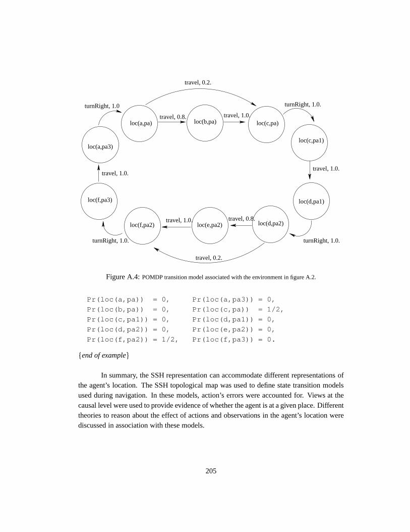
loc(a,pa) loc(b,pa)

loc(a,pa3)

loc(f,pa3)

loc(f,pa2) loc(d,pa2)

loc(d,pa1)

loc(c,pa1)

loc(c,pa)

travel, 0.2.

turnRight, 1.0.

turnRight, 1.0.

travel, 0.2.

travel, 1.0.

turnRight, 1.0

travel, 0.8. travel, 1.0.

travel, 1.0.

travel, 1.0.loc(e,pa2)

travel, 0.8.

turnRight, 1.0.

Figure A.4:POMDP transition model associated with the environment in figure A.2.

Pr(loc(a,pa)) = 0, Pr(loc(a,pa3)) = 0,

Pr(loc(b,pa)) = 0, Pr(loc(c,pa)) = 1/2,

Pr(loc(c,pa1)) = 0, Pr(loc(d,pa1)) = 0,

Pr(loc(d,pa2)) = 0, Pr(loc(e,pa2)) = 0,

Pr(loc(f,pa2)) = 1/2, Pr(loc(f,pa3)) = 0.

fend of exampleg

In summary, the SSH representation can accommodate different representations ofthe agent’s location. The SSH topological map was used to define state transition modelsused during navigation. In these models, action’s errors were accounted for. Views at thecausal level were used to provide evidence of whether the agent is at a given place. Differenttheories to reason about the effect of actions and observations in the agent’s location werediscussed in association with these models.

205

A.2 Planning

The problem of finding a sequence of actions that takes the robot from placep to placeq can be reduced to a graph search problem. This does not come as a surprise given thegraph-like structure of the SSH topological map. Paths and regions at the SSH topologicallevel are used to expedite the search for a route to a goal destination. Next we illustratehow tailored planners can be defined to efficiently use paths and regions for route finding.Generic planners can also be used with the SSH (section A.2.3).

A.2.1 Using topological paths for planning

Two basic search graphs can be associated with the SSH topological map. The first one isdefined as follows:

� The nodes of the graph are the places of the topological map.

� An edge with labelpa,dir from placep to placeq exists wheneverorder(pa; dir; p; q)is the case.

The second one is a bipartite graph such that:

� Nodes correspond to the union of places and paths in the topological map.

� An edge exists from placep to pathpa wheneveron(pa; p) is the case.

Notice that a path in the graphs above does not completely specify the sequence ofactions to get to the goal. However, enough information exists in the SSH to derive suchactions. A path on the graphs above can be easily converted to a route description, or usedas a plan skeleton during navigation.

Example 37

Consider finding a plan to go from placea to placed in the environment of figureA.5. A shortest path between these two places will be

(a; c; pa) ; (c; d; pa1) :

This path can be interpreted as the planfollow path pa until place c, then take path pa1and follow it until place d. Each of the edges in this path represents a sequence of actions:for example, the labeled edge(a; c; pa) represents the sequence of actionstravel ; travel.Turn actions need to be included in the plan when a change of path is required. For exam-ple, at placec, to turn from pathpa to pathpa1, the actionturnRightshould be executed.fend of exampleg

206

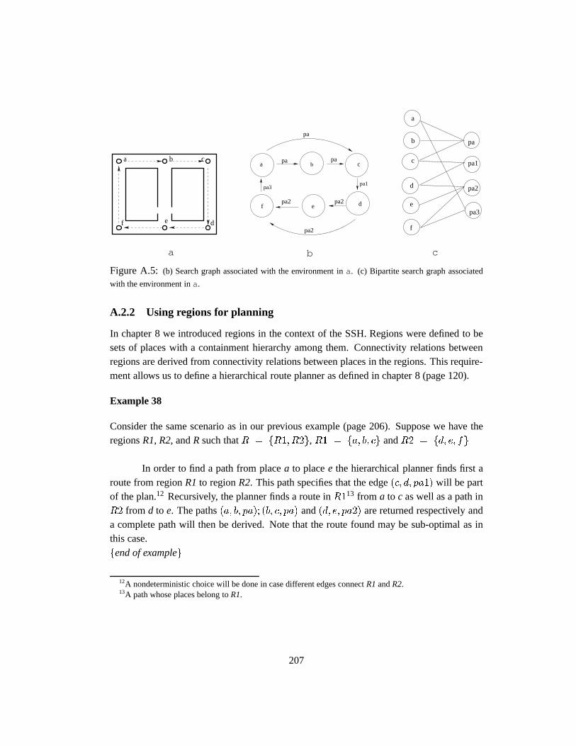
d

a

f e

b cb

pa1pa3

f e d

cpa

pa2 pa2

pa2

pa

pa

a

pa3

pa2

pa1

pa

a

b

c

d

e

f

a b c

Figure A.5: (b) Search graph associated with the environment ina. (c) Bipartite search graph associated

with the environment ina.

A.2.2 Using regions for planning

In chapter 8 we introduced regions in the context of the SSH. Regions were defined to besets of places with a containment hierarchy among them. Connectivity relations betweenregions are derived from connectivity relations between places in the regions. This require-ment allows us to define a hierarchical route planner as defined in chapter 8 (page 120).

Example 38

Consider the same scenario as in our previous example (page 206). Suppose we have theregionsR1, R2, andRsuch thatR = fR1; R2g, R1 = fa; b; cg andR2 = fd; e; fg

In order to find a path from placea to placee the hierarchical planner finds first aroute from regionR1to regionR2. This path specifies that the edge(c; d; pa1) will be partof the plan.12 Recursively, the planner finds a route inR113 from a to c as well as a path inR2 from d to e. The paths(a; b; pa); (b; c; pa) and(d; e; pa2) are returned respectively anda complete path will then be derived. Note that the route found may be sub-optimal as inthis case.fend of exampleg

12A nondeterministic choice will be done in case different edges connectR1andR2.13A path whose places belong toR1.

207

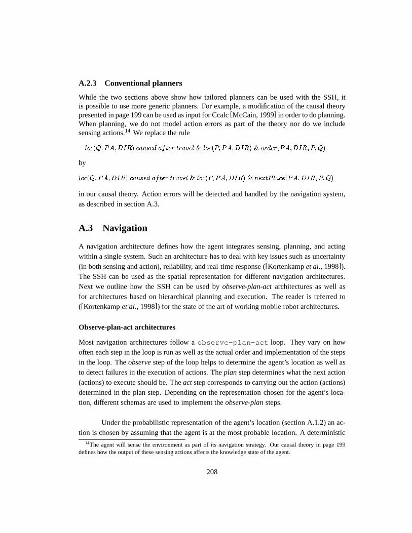
A.2.3 Conventional planners

While the two sections above show how tailored planners can be used with the SSH, itis possible to use more generic planners. For example, a modification of the causal theorypresented in page 199 can be used as input for Ccalc[McCain, 1999] in order to do planning.When planning, we do not model action errors as part of the theory nor do we includesensing actions.14 We replace the rule

loc(Q;PA;DIR) caused after travel & loc(P; PA;DIR) & order(PA;DIR; P;Q)

by

loc(Q;PA;DIR) caused after travel & loc(P; PA;DIR) & nextP lace(PA;DIR; P;Q)

in our causal theory. Action errors will be detected and handled by the navigation system,as described in section A.3.

A.3 Navigation

A navigation architecture defines how the agent integrates sensing, planning, and actingwithin a single system. Such an architecture has to deal with key issues such as uncertainty(in both sensing and action), reliability, and real-time response ([Kortenkampet al., 1998]).The SSH can be used as the spatial representation for different navigation architectures.Next we outline how the SSH can be used byobserve-plan-actarchitectures as well asfor architectures based on hierarchical planning and execution. The reader is referred to([Kortenkampet al., 1998]) for the state of the art of working mobile robot architectures.

Observe-plan-act architectures

Most navigation architectures follow aobserve-plan-act loop. They vary on howoften each step in the loop is run as well as the actual order and implementation of the stepsin the loop. Theobservestep of the loop helps to determine the agent’s location as well asto detect failures in the execution of actions. Theplan step determines what the next action(actions) to execute should be. Theactstep corresponds to carrying out the action (actions)determined in the plan step. Depending on the representation chosen for the agent’s loca-tion, different schemas are used to implement theobserve-plansteps.

Under the probabilistic representation of the agent’s location (section A.1.2) an ac-tion is chosen by assuming that the agent is at the most probable location. A deterministic

14The agent will sense the environment as part of its navigation strategy. Our causal theory in page 199defines how the output of these sensing actions affects the knowledge state of the agent.

208

plan is then generated from that location to the goal destination. The first action of suchplan is executed. Observations are made and the agent location is updated according toequation A.3. The loopobserve-plan-actcontinues until the most probable location is thedestination goal.

The description above assumes that the probability distribution has a “clear” mostprobable state. Whenever this is not the case, the agent could change its goal from going toa given destination to gathering relevant information that allows it to localize better. Oncethe agent is better localized, navigation continues to the destination goal ([Simmons andKoening, 1995, Koening and Simmons, 1998]).

When the agent’s location is represented by a set of possible locations (sectionA.1.1), the next action to execute is found by selectingl from the set of possible locations,and generating a deterministic plan froml to the destination. The first action of this plan isexecuted, observations are made and the agent’s location is updated according to equationA.1. In order to select the new current location the agent uses equation A.1 applied tothe setflg. If the result is the empty set, a new location is selected at random, otherwisea location from this set is chosen as the current location and the loopobserve-plan-actcontinues until the set of possible locations is a subset of the set of locations satisfiyingthe goal. The reader is referred to[Nourbakhsh and Genesereth, 1996, Nourbakhsh, 1998,Baral and Gelfond, 1999] for details on how to implement these ideas.

Hierarchical planning and execution

Hierarchical planning as described in section A.2.2 can be interleaved with plan executionto efficiently accommodate errors in actions and sensing as well as incomplete information.Instead of generating a detailed plan, thehierarchical plannerrepresents a plan by a treewhose nodes get expanded as the plan is executed. This tree is traversed in a depth firstfashion so that actions for the robot can be generated as soon as possible.

Each node of the plan tree represents a plan step that theplannertells thesequencerto execute. The sequencer either executes this plan step and notifies the planner it did soor asksthe planner for more information on how to carry on the step. On receiving a no-tification from the sequencer, the planner either tells the agent to execute the next step inthe plan (if the sequencer successfully executed the previous step) or search for a new planto achieve the goal. On being asked for more information about a plan step, the plannerexpands the plan step and tells the sequencer to execute a new (probably more refined) stepin the plan. The net result of thetell/ask interaction between the planner and the se-

209

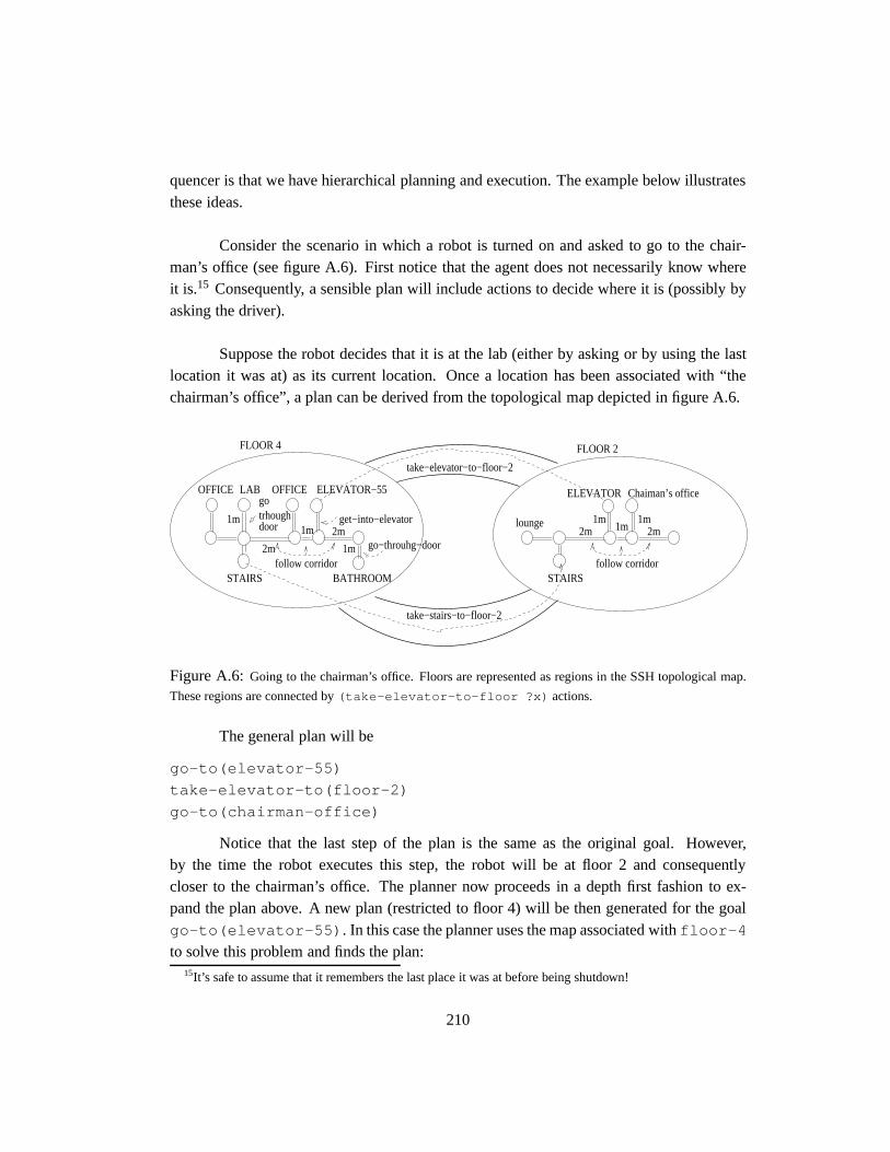
quencer is that we have hierarchical planning and execution. The example below illustratesthese ideas.

Consider the scenario in which a robot is turned on and asked to go to the chair-man’s office (see figure A.6). First notice that the agent does not necessarily know whereit is.15 Consequently, a sensible plan will include actions to decide where it is (possibly byasking the driver).

Suppose the robot decides that it is at the lab (either by asking or by using the lastlocation it was at) as its current location. Once a location has been associated with “thechairman’s office”, a plan can be derived from the topological map depicted in figure A.6.

2m

FLOOR 2

2m2m1m 1m

1m

follow corridorSTAIRS

lounge

ELEVATOR Chaiman’s office

FLOOR 4

STAIRS BATHROOM

go−throuhg−door1mfollow corridor

1m get−into−elevator

goOFFICE LAB OFFICE ELEVATOR−55

trhough

2m

door 1m

take−elevator−to−floor−2

take−stairs−to−floor−2

Figure A.6: Going to the chairman’s office. Floors are represented as regions in the SSH topological map.

These regions are connected by(take-elevator-to-floor ?x) actions.

The general plan will be

go-to(elevator-55)

take-elevator-to(floor-2)

go-to(chairman-office)

Notice that the last step of the plan is the same as the original goal. However,by the time the robot executes this step, the robot will be at floor 2 and consequentlycloser to the chairman’s office. The planner now proceeds in a depth first fashion to ex-pand the plan above. A new plan (restricted to floor 4) will be then generated for the goalgo-to(elevator-55) . In this case the planner uses the map associated withfloor-4

to solve this problem and finds the plan:15It’s safe to assume that it remembers the last place it was at before being shutdown!

210

go-through-door

follow-corridor for about 2m

follow-corridor for about 1m

Whether the robot should go left or right at the corridor after going through the dooris not explicitly mentioned in the plan. That information will be made explicit during theplan execution. In order to execute the plan above, the planner tells the sequencer to executeeach plan step as follows:16

(define-sequencer-task (step-go-through-door)

(if (succeed (go-through-door))

(notify-planner success)

(ask-planner expand-step))

)

The (notify-planner success) call allows the planner to monitor the ex-ecution of the plan. As steps are executed, the robot’s location in the map is updated. Onreceiving a notification of step execution success, the planner will invoke the execution ofthe next step in the plan (by generating a plan step similar to the one above).

When the planner is asked toexpanda plan step, it uses a more detailed map tocarry out the step. If this is not possible, a failure in the plan is detected. Failures are takeninto account by indicating that either a place or path in the topological map cannot be usedfor future plans.17 For example, if the plan step(go-through-door) fails, then therobot should conclude that it is still at the lab, and that the path connecting the lab with thecorridor should not be used for future plans.

The actiongo-through-door looks like

(define-sequencer-task (go-through-door)

(if (look-and-found? ?door)

((get-close-to ?door) (pass-through ?door))

(return failure)

)

)16For the purpose of the examples we made up a language to specify the tasks the sequencer should carry on.

Special purpose languages exist to specify these tasks: RAPS[Firby, 1994], ESL[Gat, 1996]. See[Kortenkampet al., 1998].

17This implies that the planner has a local memory to indicate changes in the representation.

211

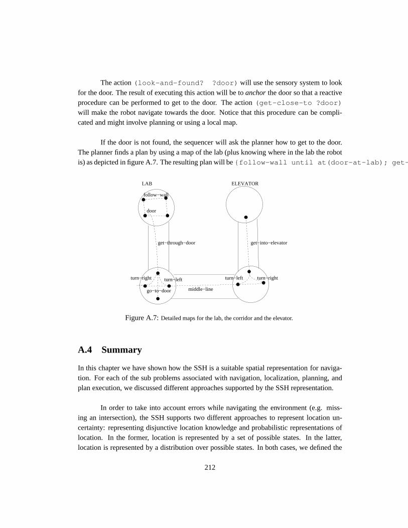
The action(look-and-found? ?door) will use the sensory system to lookfor the door. The result of executing this action will be toanchorthe door so that a reactiveprocedure can be performed to get to the door. The action(get-close-to ?door)

will make the robot navigate towards the door. Notice that this procedure can be compli-cated and might involve planning or using a local map.

If the door is not found, the sequencer will ask the planner how to get to the door.The planner finds a plan by using a map of the lab (plus knowing where in the lab the robotis) as depicted in figure A.7. The resulting plan will be{follow-wall until at(door-at-lab); get -

go−to−door

turn−left

middle−line

ELEVATORLAB

door

get−through−door

follow−wall

turn−right turn−rightturn−left

get−into−elevator

Figure A.7:Detailed maps for the lab, the corridor and the elevator.

A.4 Summary

In this chapter we have shown how the SSH is a suitable spatial representation for naviga-tion. For each of the sub problems associated with navigation, localization, planning, andplan execution, we discussed different approaches supported by the SSH representation.

In order to take into account errors while navigating the environment (e.g. miss-ing an intersection), the SSH supports two different approaches to represent location un-certainty: representing disjunctive location knowledge and probabilistic representations oflocation. In the former, location is represented by a set of possible states. In the latter,location is represented by a distribution over possible states. In both cases, we defined the

212

transition and observation models associated with the corresponding approaches.

In order to solve planning problems (i.e. finding a route to a goal destination), theSSH supports the use of standard planners as well as special purpose planners exploitingpaths and regions at the SSH topological level. We defined the corresponding algorithmsfor this later case.

Finally, we discussed different navigation architectures supported by the SSH. Inaddition to observe-plan-act architectures, we defined an architecture combining hierarchi-cal planning and execution. In this architecture, instead of generating a detailed plan, ahierarchical planner represents a plan by a tree whose nodes get expanded as the plan isexecuted. This tree is traversed in a depth first fashion so that actions for the robot can begenerated as soon as possible. We illustrated how this architecture can accomodate recur-sive plans (i.e. in order to go home, leave the office and go home) as well as recover fromerrors in action execution.

The different methods described in this chapter illustrate how the SSH supportsnavigation. In addition, the methods illustrate how the different SSH levels are combinedduring localization, planning and plan-execution.

213

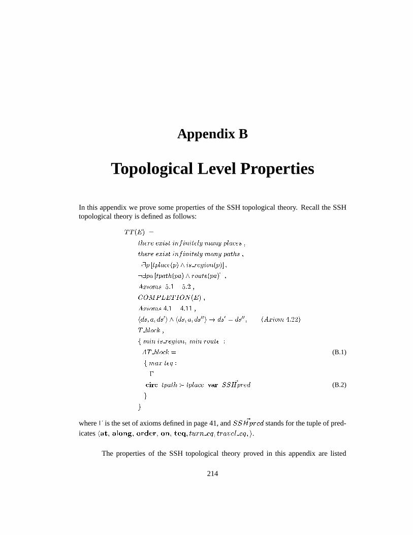
Appendix B

Topological Level Properties

In this appendix we prove some properties of the SSH topological theory. Recall the SSHtopological theory is defined as follows:

TT (E) =

there exist infinitely many places ;

there exist infinitely many paths ;

:9p [tplace(p) ^ is region(p)] ;

:9pa [tpath(pa) ^ route(pa)] ;

Axioms 5:1� 5:2 ;

COMPLETION(E) ;

Axioms 4:1� 4:11 ;

hds; a; ds0i ^ hds; a; ds00i ! ds0 = ds00; (Axiom 4:22)

T block ;

f min is region; min route :

AT block = (B.1)

f max teq :

�

circ tpath � tplace var ~SSHpred (B.2)

g

g

where� is the set of axioms defined in page 41, and ~SSHpred stands for the tuple of pred-icateshat; along; order; on; teq; turn eq; travel eq; i.

The properties of the SSH topological theory proved in this appendix are listed

214

below. LetM be a model forTT (E), then

� M j= 8pa; [tpath(pa) � 9ds; dir along(ds; pa; dir)].

� M j= 8p; [tplace(p) � 9ds at(ds; p)].

� The topological map associated with a finite set of experiencesE has a finite numberof topological paths and a finite number of topological places.

� Any two models of the SSH topological theory have the same number of topologicalpaths and the same number of topological places.

Theorem 8 LetM be a model ofTT (E). Then,

� M j= 8pa; [tpath(pa) � 9ds; dir along(ds; pa; dir)].

� M j= 8p; [tplace(p) � 9ds at(ds; p)].

Proof.

CIRC[�; tpath � tplace;SSHpred]

� fproposition 15 in [Lifschitz; 1994]g

CIRC[�; tpath; tplace; SSHpred] ^ CIRC[�; tpath; tplace;SSHpred]

! fdef: of circumscriptiong

CIRC[�; tpath]

Since� = �0(tpath) ^ [along(ds; pa; dir) ! tpath(pa)] where�0(tpath) is neg-ative, then

CIRC[�; tpath]

�

CIRC[�0(tpath) ^ [along(ds; pa; dir)! tpath(pa)]; tpath]

� fproposition 4 in [Lifschitz; 1994]g

�0(tpath) ^ CIRC[along(ds; pa; dir)! tpath(pa); tpath]

! fproposition 1 in [Lifschitz; 1994]g

[9ds; dir along(ds; pa; dir)] � tpath(pa)

Similarly, � = �0 ^ [at(ds; p) ! tplace(p)] wheretpath does not occur in�0.Then,

CIRC[�; tpath � tplace;SSHpred]

215

! fsee aboveg

CIRC[�; tpath; tplace;SSHpred]

! fdef: parallel circumscriptiong

CIRC[�; tpath; tplace]

! fdef: parallel circumscriptiong

CIRC[�0 ^ [at(ds; p)! tplace(p)]; tplace]

� fpropositions 1 and 4 in [Lifschitz; 1994]g

�0 ^ [9ds; at(ds; p)] � tplace(p)

2

Theorem 4. The topological map associated with a finite set of experiencesE hasa finite number of topological paths and a finite number of topological places.

Proof. Since a distinctive state is along at most one topological path (axiom 5.24,page 42), theorem 8 implies that for any modelM of TT (E) there is an injection fromtpathM into distinctive-statesM . Sincedistinctive-statesM is finite so istpathM .

Similarly, since distinctive states are at a unique topological place (axiom 5.16, page41), from theorem 8 we conclude that the set of topological places in a model ofTT (E) isfinite. 2

Theorem 5. Any two models of the SSH topological theory have the same numberof topological paths and the same number of topological places.

Proof. In order to prove that two modelsM1 andM2 of TT (E) have the samenumber of topological paths (tpaths) and the same number of topological places (tplaces), itis enough to show that this is the case for models of theAT block (block B.1). Suppose thattpathM1 has less elements thantpathM2 , and so there exists an injection� : tpathM1 !

tpathM2 . One can extend� to define an isomorphism fromM1 into M 02, such thatM 02 �M2, where� is the order defined by the circumscription policy B.2.1 In fact,

� Let � : tplaceM1 ! placesM2 be an injection. Such an injection exists sincetplaceM1 is finite andplacesM2 is infinite.

� Let � : SM1 ! SM2 be the identity over the sorts (S)of distinctive states, actions,1This proves thatM1 andM2 have the same number of topological paths.

216

views, schemas, path types and path directions. Recall we assumed aHerbrand in-terpretation for these sorts, where the corresponding universes are defined by theconstant symbols inE.

The function� above defines an isomorphic embedding fromM1 into M2 in thestandard way. In fact,�(M1) =M 02 is defined as follows:

� tpathM0

2 = �(tpathM1), tplaceM0

2 = �(tplaceM1).

� teqM0

2 = �(teqM1) = fteq(ds1; ds2) : M1 j= teq(ds1; ds2)g = teqM1 .

� atM0

2 = �(atM1) = fat(ds; �(p)) : M1 j= at(ds; p)g.

� alongM0

2 = �(alongM1) = falong(ds; �(pa); dir) : M1 j= along(ds; pa; dir)g.

� orderM0

2 =�(orderM1 ) =forder(�(pa); dir; �(p); �(q)) :M1 j= order(pa; dir; p; q)g.

� onM0

2 = �(onM1 ) = fon(�(pa); �(p)) : M1 j= on(pa; p)g.

� turn eqM0

2 = �(turn eqM1) = turn eqM1.

� travel eqM0

2 = �(travel eqM1) = travel eqM1.

Notice that the language of� is defined byftpath; tplaceg [ SSHpred. ThusM1 j= � implies�(M1) j= �.2 Since�(tpathM1) � tpathM2 , then�(M1) � M2, andsoM2 is not minimal, and is therefore not a model ofTT (E). It follows thatM1 andM2

have the same number of topological paths.

Similar argument shows thatM1 andM2 have the same number of topologicalplaces. If not, there would exists� : tpathM1 ! tpathM2 a bijection and� : tplaceM1 !

tplaceM2 an injection that allows us to apply the same argument as above.2

Theorem 6. Let ds1 be a distinctive state symbol such that

8ds2 62 [ds1]dturn; [ds2]teq \ [ds1]dturn = ; : (B.3)

Then8ds2 62 [ds1]dturn; place(ds2) 6= place(ds1) :

2Notice that the circumscription policy varies all predicates in the language of�, and� is the identityover all constant symbols in the theory, for otherwise,�(M1) j= � is not necessarily the case. In generalthe interpretations of a unary predicate (set) under a circumscriptive theory do not have the same number ofelements. For example, consider the models ofCIRC[(P (0)^ P (1)) _ P (2);P ], where the interpretation ofP could have one or two elements (this example is due to Vladimir Lifschitz).

217

Proof. The hypothesis of the theorem implies that

8ds2 62 [ds1]dturn; :turn eq(ds2; ds1) :

Indeed,

turn eq(ds1; ds2)

�

9b0; : : : ; bn; b00 ; : : : ; bn0 s:t:

� b0 = ds2; bn0 = ds1 ;

� teq(bi; bi0); i = 0; : : : ; n

� dturn(bi0 ; bi+1); i = 0; : : : ; n� 1 :

Let 1 � j � n such thath8j � k � n; bk0 2 [ds1]dturni andb(j�1)0 62 [ds1]dturn.

Notice that such aj exists sinceds1 = b00 62 [ds1]dturn and ds1 = bn0 2 [ds1]dturn.Consequently,

turn eq(ds1; ds2)

!

bj0 2 [ds1]dturn! fteq(bj ; bj0)g

[bj ]teq \ [ds1]dturn 6= ;! fB:3g

bj 2 [ds1]dturn! fdturn(b(j�1)0 ; bj)gb(j�1)0 2 [ds1]dturn!

false

Thus:turn eq(ds2; ds1) should be the case.2

218

Appendix C

Nested Abnormality theories

In this appendix we define circumscription and nested abnormalities theories following[Lifschitz, 1994, Lifschitz, 1995].

The main idea of circumscription is to consider, instead of arbitrary models of anaxiom set, only the models that satisfy a certain minimality condition (usually set inclu-sion). Mathematically, circumscription is defined as a syntactic transformation of logicalformulas. It transforms a sentenceA into a stronger sentenceA�, such that the models ofA� are precisely the minimal models ofA.

Definition 12 (Circumscription)

LetA(P;Z1; : : : ; Zm) be a sentence containing a predicate constantP and object, functionand/or predicate constantsZ1; : : : ; Zm (and possibly other object, function and predicateconstants). Thecircumscription of P in A with variedZ1; : : : ; Zm is the sentence

A(P;Z1; : : : ; Zm) ^ :9p; z1; : : : ; zm [A(p; z1; : : : ; zm) ^ p < P ] (C.1)

wherep < P denotes the formula

8x fp(x)! P (x)g ^ 9x f:p(x) ^ P (x)g :

We denote formula C.1 byCIRC [A;P ;Z].fend of definitiong

Intuitively, the models ofCIRC [A;P ;Z] are the models ofA in which the extentof P cannot be smaller without losing the propertyA, even at the price of changing the

219

interpretations of the constantsZ. In order to make this claim precisely, the followingorder,�P ;Z, is defined among structures of the language ofA.

Definition 13 (�P ;Z)

Let M1 andM2 be two structures for a given one-sorted language. ThenM1 �P ;Z M2

whenever

� jM1j = jM2j,1

� M1 [C] = M2 [C],2 for every constantC which is different fromP and does notbelong toZ,

� M1 [P ] �M2 [P ]

fend of definitiong

In other words,M1 �P ;Z M2 means thatM1 andM2 differ only in how they

interpretP andZ, and the extent ofP in M1 is a subset of its extent inM2. Proposition 1in [Lifschitz, 1994] states that

Theorem 9 A structureM is a model ofCIRC [A;P ;Z] if and only if M is minimalrelative to�P ;Z.

Example 39

Circumscription is usually used in order to formalize default associated with an axiomatictheory. Suppose the we would like to represent the default “Normally a block in on thetable”. Suppose blockB1 is not on the table and letB2 denotes another block. The circum-scriptive theory below allow us to concludeOntable(B2):

Block(x) ^ :Ab(x)! Ontable(x) (C.2)

:Ontable(B1) (C.3)

Block(B1); Block(B2); B1 6= B2 (C.4)

circ Ab var Ontable (C.5)

where we have extended our notation such that the above should be understood as

CIRC [C:2 ^ C:3 ^ C:4;Ab;Ontable] :

1For a structureM , jM j denotes the universe ofM .2M [C] denotes the interpretation ofC in M .

220

In the above theory, it is the case thatAb(x) � x = B1, and consequentlyOntable(B2)

follows. The role of the predicateAb is to single out the blocks that are“abnormal” relativeto the default (C.2).fend of exampleg

It is often convenient to arrange different defaults by assigning priorities to them.For example, consider formalizing the enhancement of the theory above in which “Blocksare usually heavy”, and “heavy block are usually not in the table”. Next we define two ex-tensions to the basic definition of circumscription: parallel and prioritized circumscription.

Definition 14 (Parallel Circumscription)

Theparallel circumscription

CIRChA;P 1; : : : ; P n;Z

iis the sentence

A(P;Z) ^ :9p; z [A(p; z) ^ p � P ] ;

whereP stands for the tuple of predicatesP 1; : : : ; P n andp � P stands for the formula8 1 � i � n pi � P i ^ 9 1 � i � n pi < P i

fend of definitiong

The parallel circumscription of several predicates has a simple model theoreticscharacterization, similar to the one presented by theorem 9. WhenP is a tupleP 1; : : : ; P n,the relationM1 �

P ;Z M2 between structuresM1 andM2 is defined as before, except thatthe conditionM1 [P ] �M2 [P ] is replaced byM1

�P i��M2

�P i�

for all i = 1; : : : ; n.

Definition 15 (Prioritized Circumscription)

Theprioritized circumscription

CIRChA;P 1 � : : : � P n;Z

iis the sentence

A(P;Z) ^ :9p; z [A(p; z) ^ p � P ] ;

whereP stands for the tuple of predicatesP 1; : : : ; P n andp � P stands for the formula

n_i=1

0@i�1

j=1

(pj = P j) ^ (pi < P i)

1A :

221

fend of definitiong

The formulap � P defines alexicographicorder among the predicates inp andP .Whenk = 1 it becomesp < P ; if k = 2, it becomes

(p1 < P 1) _ ((p1 = P 1)! (p2 < P 2)) :

Proposition 15 in[Lifschitz, 1994] shows that prioritized circumscription can be reduced toparallel circumscription as follows:

Theorem 10 The circumscriptionCIRC�A;P 1 � : : : � P n;Z

�is equivalent to

n

i=1

CIRChA;P i;P i+1; : : : ; P n; Z

i:

Notation 2

CIRC�A;P 1 � : : ::Pi : : : � P n;Z

�stands for the formula

CIRChA ^ not Pi � :Pi;P

1 � : : : not Pi : : : � P n;Z;Pii

wherenot Pi is a new constant predicate not occurring inA. fend of notationg

C.1 Nested Abnormality theories (NAT’s)

Nested abnormality theories allows one to apply the circumscription operator to a subsetof axioms, by structuring the knowledge base (the theory) into blocks. Each block can beviewed as a group of axioms that describes a certain collection of predicates and functions,and the nesting of blocks reflects the dependence of these descriptions on each other.

Definition 16 (NAT’s)

Consider a second-order languageL that doesnot includeAb among its symbols. For ev-ery natural numberk, by Lk we denote the language obtained fromL by addingAb as ak-ary predicate constant.Blocksare defined recursively as follows: For anyk and any listof function and/or predicate constantsC1; : : : ; Cm of L, if each ofA1; : : : ; An is a formulaof Lk or ablock, thenfC1; : : : ; Cm : A1; : : : ; Ang is ablock. The last expression reads:C1; : : : ; Cm are such thatA1; : : : ; An. AboutC1; : : : ; Cm we say that they aredescribed

222

by this block.

The semantics of NAT’s is characterized by a map' that translates blocks intosentences ofL. It is convenient to make' defined also on formulas of the languagesLk. IfA is such a formula, then'(A) stands for the universal closure ofA. For blocks we define,recursively:

' fC1; : : : ; Cm : A1; : : : ; Ang = 9ab CIRC ['A1; : : : ; 'An : ab : C1; : : : ; Cm] :

fend of definitiong

Example 40

Consider the standard example: objects normally don’t fly: birds normally do; canaries arebirds; Tweety is a canary. These assertions can be formalized as the NAT whose only axiomis

fF lies :

F lies(x)! Ab(x);

f F lies :

Bird(x) ^ :Ab(x)! F lies(x);

Canary(x)! Bird(x);

Canary(Tweety)

g

g

The outer block describe the ability of objects to fly; the inner block gives more specific in-formation about the ability ofbirds to fly. Each occurrence of the predicateAb is “local” toits block, and so, the two occurrences of the predicateAb refer two “unrelated” predicatesthough we use the same name.fend of exampleg

Most often, it is desirable not to mention the predicateAb at all. We will adopt thefollowing notations:

� fC1; : : : ; Cm;min P : A1; : : : ; Ang stands for

fC1; : : : ; Cm; P : P (x)! Ab(x); A1; : : : ; Ang

223

� fC1; : : : ; Cm;max P : A1; : : : ; Ang stands for

fC1; : : : ; Cm; P : :Ab(x)! P (x); A1; : : : ; Ang

Using this notation, we could rewrite our previous example as

fmin F lies :

f F lies :

Bird(x) ^ :Ab(x)! F lies(x);

Canary(x)! Bird(x);

Canary(Tweety)

g

g

where we dispense the occurrence of oneAb predicate. The reader is referred to[McCarthy, 1980, McCarthy, 1986, Lifschitz, 1994, Lifschitz, 1995] for a complete surveyof the uses and properties of circumscriptions and NATs.

Definition 17

We extend the definition ofblocksas follows: ifA is a block, so isCIRC[A;P 1 � : : : �

P n;Z]. The semantics of NATs is extended such that

�CIRC[A;P 1 � : : : � P n;Z] = CIRC[�A;P 1 � : : : � P n;Z] :

fend of notationg

As the next theorem shows, in some cases prioritized circumscription can be ex-pressed using NAT’s. In these cases however, the notation for prioritized circumscription ismore compact than its equivalent NAT’s. This motivates our previous definition.

Theorem 11 LetA be a sentence such thatAb does not occur inA. Then,

CIRC[A;P � Q;Z] = fZ; min Q : fZ; Q; min P : A g g :

Proof.

fZ; minQ : fZ; Q; minP : A g g

224

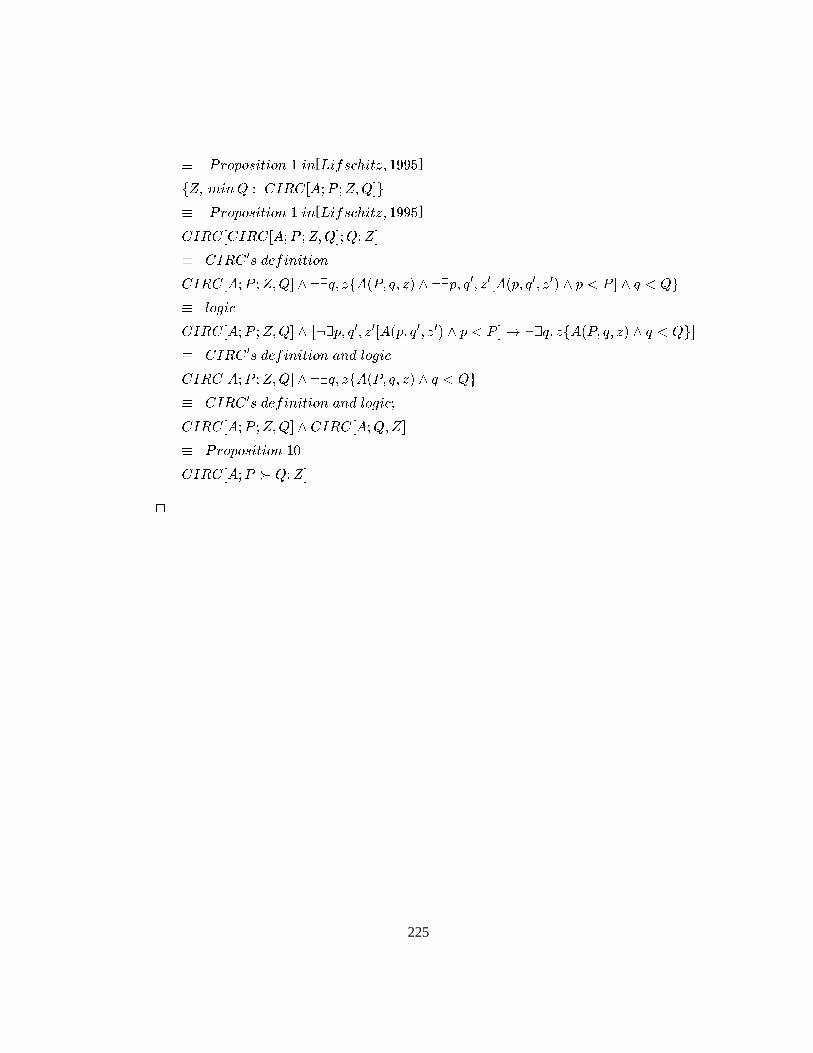
� Proposition 1 in[Lifschitz; 1995]

fZ; minQ : CIRC[A;P ;Z;Q]g

� Proposition 1 in[Lifschitz; 1995]

CIRC[CIRC[A;P ;Z;Q];Q;Z]

� CIRC 0s definition

CIRC[A;P ;Z;Q] ^ :9q; zfA(P; q; z) ^ :9p; q0; z0[A(p; q0; z0) ^ p < P ] ^ q < Qg

� logic

CIRC[A;P ;Z;Q] ^�:9p; q0; z0[A(p; q0; z0) ^ p < P ]! :9q; zfA(P; q; z) ^ q < Qg

�� CIRC 0s definition and logic

CIRC[A;P ;Z;Q] ^ :9q; zfA(P; q; z) ^ q < Qg

� CIRC 0s definition and logic;

CIRC[A;P ;Z;Q] ^ CIRC[A;Q;Z]

� Proposition 10

CIRC[A;P � Q;Z]

2

225

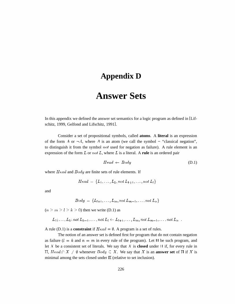
Appendix D

Answer Sets

In this appendix we defined the answer set semantics for a logic program as defined in[Lif-schitz, 1999, Gelfond and Lifschitz, 1991].

Consider a set of propositional symbols, calledatoms. A literal is an expressionof the formA or :A, whereA is an atom (we call the symbol: “classical negation”,to distinguish it from the symbolnot used for negation as failure). A rule element is anexpression of the formL or notL, whereL is a literal. Arule is an ordered pair

Head Body (D.1)

whereHead andBody are finite sets of rule elements. If

Head = fL1; : : : ; Lk; not Lk+1; : : : ; not Llg

and

Body = fLl+1; : : : ; Lm; not Lm+1; : : : ; not Lng

(n � m � l � k � 0) then we write (D.1) as

L1; : : : ; Lk;notLk+1; : : : ; not Ll Ll+1; : : : ; Lm; not Lm+1; : : : ; not Ln :

A rule (D.1) is aconstraint if Head = ;. A program is a set of rules.The notion of an answer set is defined first for program that do not contain negation

as failure (l = k andn = m in every rule of the program). Let� be such program, andlet X be a consistent set of literals. We say thatX is closedunder� if, for every rule in�, Head \ X 6= ; wheneverBody � X. We say thatX is ananswer setof � if X isminimal among the sets closed under� (relative to set inclusion).

226

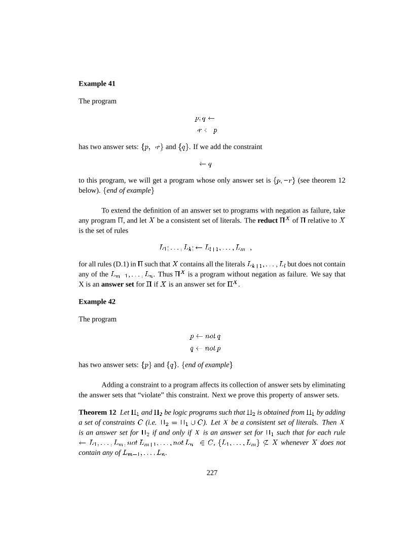
Example 41

The program

p; q

:r p

has two answer sets:fp;:rg andfqg. If we add the constraint

q

to this program, we will get a program whose only answer set isfp;:rg (see theorem 12below).fend of exampleg

To extend the definition of an answer set to programs with negation as failure, takeany program�, and letX be a consistent set of literals. Thereduct �X of � relative toXis the set of rules

L1; : : : ; Lk; Ll+1; : : : ; Lm ;

for all rules (D.1) in� such thatX contains all the literalsLk+1; : : : ; Ll but does not containany of theLm+1; : : : ; Ln. Thus�X is a program without negation as failure. We say thatX is ananswer setfor � if X is an answer set for�X .

Example 42

The program

p not q

q not p

has two answer sets:fpg andfqg. fend of exampleg

Adding a constraint to a program affects its collection of answer sets by eliminatingthe answer sets that “violate” this constraint. Next we prove this property of answer sets.

Theorem 12 Let�1 and�2 be logic programs such that�2 is obtained from�1 by addinga set of constraintsC (i.e. �2 = �1 [ C). LetX be a consistent set of literals. ThenXis an answer set for�2 if and only ifX is an answer set for�1 such that for each rule L1; : : : ; Lm; not Lm+1; : : : ; not Ln 2 C, fL1; : : : ; Lmg 6� X wheneverX does notcontain any ofLm+1; : : : ; Ln.

227

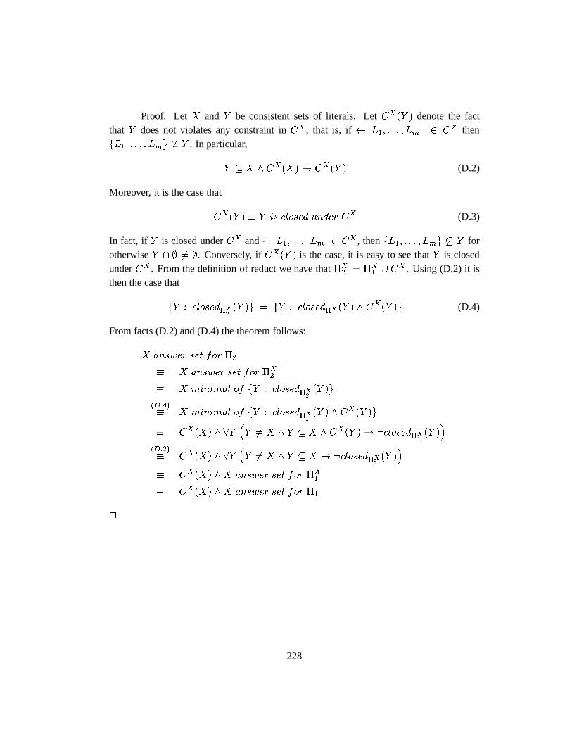
Proof. LetX andY be consistent sets of literals. LetCX(Y ) denote the factthat Y does not violates any constraint inCX , that is, if L1; : : : ; Lm 2 CX thenfL1; : : : ; Lmg 6� Y . In particular,

Y � X ^ CX(X)! CX(Y ) (D.2)

Moreover, it is the case that

CX(Y ) � Y is closed under CX (D.3)

In fact, if Y is closed underCX and L1; : : : ; Lm 2 CX , thenfL1; : : : ; Lmg 6� Y forotherwiseY \ ; 6= ;. Conversely, ifCX(Y ) is the case, it is easy to see thatY is closedunderCX . From the definition of reduct we have that�X

2 = �X1 [ C

X . Using (D.2) it isthen the case that

fY : closed�X2(Y )g = fY : closed�X

1(Y ) ^ CX(Y )g (D.4)

From facts (D.2) and (D.4) the theorem follows:

X answer set for �2

� X answer set for �X2

� X minimal of fY : closed�X2(Y )g

(D:4)� X minimal of fY : closed�X

1(Y ) ^CX(Y )g

� CX(X) ^ 8Y�Y 6= X ^ Y � X ^ CX(Y )! :closed�X

1(Y )

�(D:2)� CX(X) ^ 8Y

�Y 6= X ^ Y � X ! :closed�X

1(Y )

�� CX(X) ^X answer set for �X

1

� CX(X) ^X answer set for �1

2

228

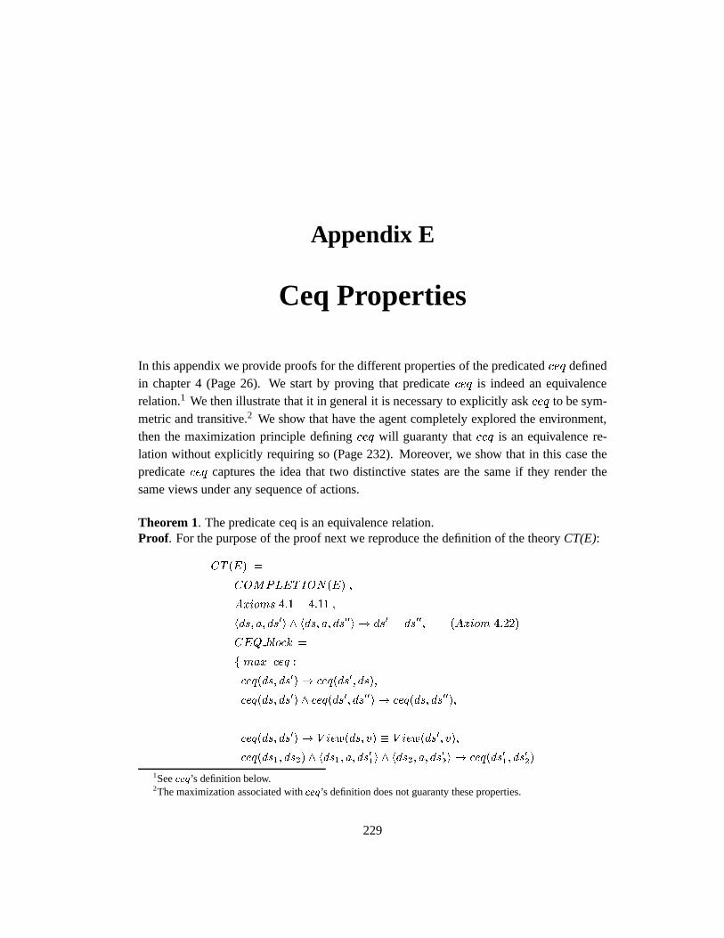
Appendix E

Ceq Properties

In this appendix we provide proofs for the different properties of the predicatedceq definedin chapter 4 (Page 26). We start by proving that predicateceq is indeed an equivalencerelation.1 We then illustrate that it in general it is necessary to explicitly askceq to be sym-metric and transitive.2 We show that have the agent completely explored the environment,then the maximization principle definingceq will guaranty thatceq is an equivalence re-lation without explicitly requiring so (Page 232). Moreover, we show that in this case thepredicateceq captures the idea that two distinctive states are the same if they render thesame views under any sequence of actions.

Theorem 1. The predicate ceq is an equivalence relation.Proof. For the purpose of the proof next we reproduce the definition of the theoryCT(E):

CT (E) =

COMPLETION(E) ;

Axioms 4:1� 4:11 ;

hds; a; ds0i ^ hds; a; ds00i ! ds0 = ds00; (Axiom 4:22)

CEQ block =

f max ceq :

ceq(ds; ds0)! ceq(ds0; ds);

ceq(ds; ds0) ^ ceq(ds0; ds00)! ceq(ds; ds00);

ceq(ds; ds0)! V iew(ds; v) � V iew(ds0; v);

ceq(ds1; ds2) ^ hds1; a; ds0

1i ^ hds2; a; ds0

2i ! ceq(ds01; ds0

2)

1Seeceq’s definition below.2The maximization associated withceq’s definition does not guaranty these properties.

229

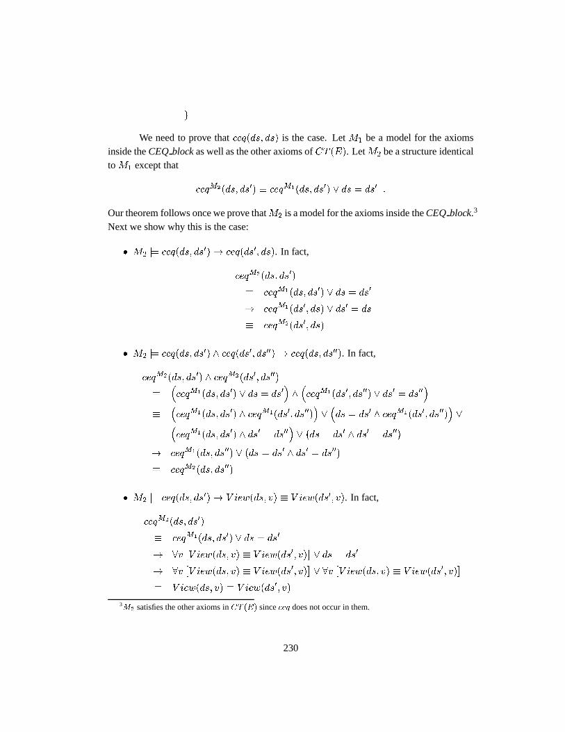
g

We need to prove thatceq(ds; ds) is the case. LetM1 be a model for the axiomsinside theCEQ blockas well as the other axioms ofCT (E). LetM2 be a structure identicaltoM1 except that

ceqM2(ds; ds0) � ceqM1(ds; ds0) _ ds = ds0 :

Our theorem follows once we prove thatM2 is a model for the axioms inside theCEQ block.3

Next we show why this is the case:

� M2 j= ceq(ds; ds0)! ceq(ds0; ds). In fact,

ceqM2(ds; ds0)

� ceqM1(ds; ds0) _ ds = ds0

! ceqM1(ds0; ds) _ ds0 = ds

� ceqM2(ds0; ds)

� M2 j= ceq(ds; ds0) ^ ceq(ds0; ds00)! ceq(ds; ds00). In fact,

ceqM2(ds; ds0) ^ ceqM2(ds0; ds00)

��ceqM1(ds; ds0) _ ds = ds0

�^�ceqM1(ds0; ds00) _ ds0 = ds00

��

�ceqM1(ds; ds0) ^ ceqM1(ds0; ds00)

�_�ds = ds0 ^ ceqM1(ds0; ds00)

�_�

ceqM1(ds; ds0) ^ ds0 = ds00�_�ds = ds0 ^ ds0 = ds00

�! ceqM1(ds; ds00) _

�ds = ds0 ^ ds0 = ds00

�� ceqM2(ds; ds00)

� M2 j= ceq(ds; ds0)! V iew(ds; v) � V iew(ds0; v). In fact,

ceqM2(ds; ds0)

� ceqM1(ds; ds0) _ ds = ds0

! 8v�V iew(ds; v) � V iew(ds0; v)

�_ ds = ds0

! 8v�V iew(ds; v) � V iew(ds0; v)

�_ 8v

�V iew(ds; v) � V iew(ds0; v)

�� V iew(ds; v) � V iew(ds0; v)

3M2 satisfies the other axioms inCT (E) sinceceq does not occur in them.

230

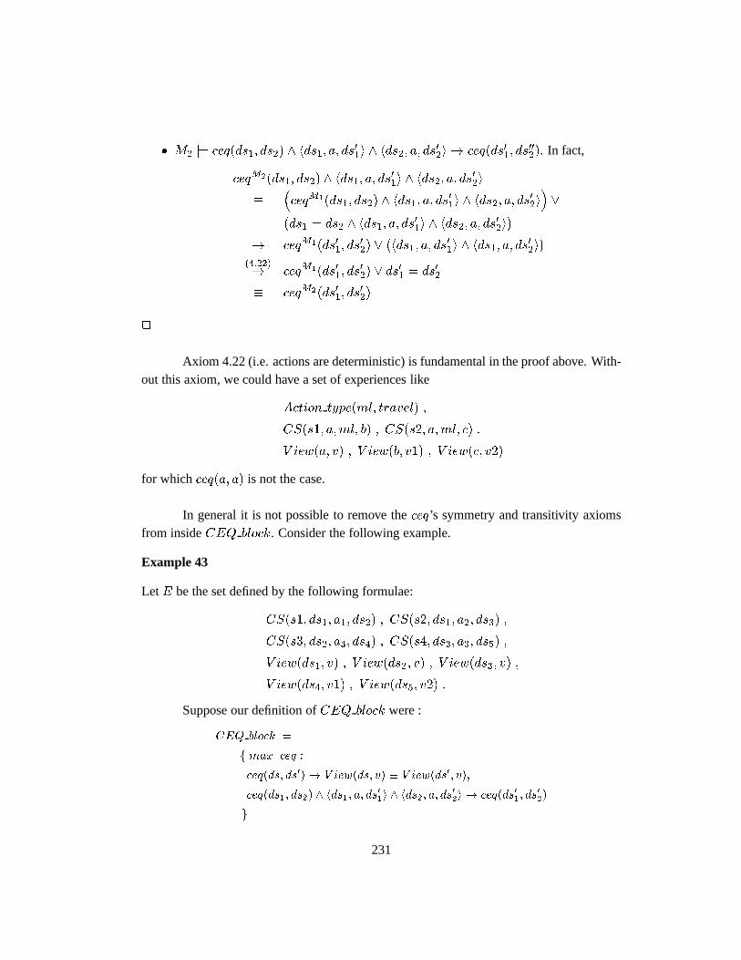
� M2 j= ceq(ds1; ds2) ^ hds1; a; ds01i ^ hds2; a; ds

02i ! ceq(ds01; ds

002). In fact,

ceqM2(ds1; ds2) ^ hds1; a; ds01i ^ hds2; a; ds

02i

��ceqM1(ds1; ds2) ^ hds1; a; ds

01i ^ hds2; a; ds

02i�_�

ds1 = ds2 ^ hds1; a; ds01i ^ hds2; a; ds

02i�

! ceqM1(ds01; ds02) _

�hds1; a; ds

01i ^ hds1; a; ds

02i�

(4:22)! ceqM1(ds01; ds

02) _ ds

01 = ds02

� ceqM2(ds01; ds02)

2

Axiom 4.22 (i.e. actions are deterministic) is fundamental in the proof above. With-out this axiom, we could have a set of experiences like

Action type(ml; travel) ;

CS(s1; a;ml; b) ; CS(s2; a;ml; c) :

V iew(a; v) ; V iew(b; v1) ; V iew(c; v2)

for which ceq(a; a) is not the case.

In general it is not possible to remove theceq’s symmetry and transitivity axiomsfrom insideCEQ block. Consider the following example.

Example 43

LetE be the set defined by the following formulae:

CS(s1; ds1; a1; ds2) ; CS(s2; ds1; a2; ds3) ;

CS(s3; ds2; a3; ds4) ; CS(s4; ds3; a3; ds5) ;

V iew(ds1; v) ; V iew(ds2; v) ; V iew(ds3; v) ;

V iew(ds4; v1) ; V iew(ds5; v2) :

Suppose our definition ofCEQ block were :

CEQ block =

f max ceq :

ceq(ds; ds0)! V iew(ds; v) � V iew(ds0; v);

ceq(ds1; ds2) ^ hds1; a; ds0

1i ^ hds2; a; ds0

2i ! ceq(ds01; ds0

2)

g

231

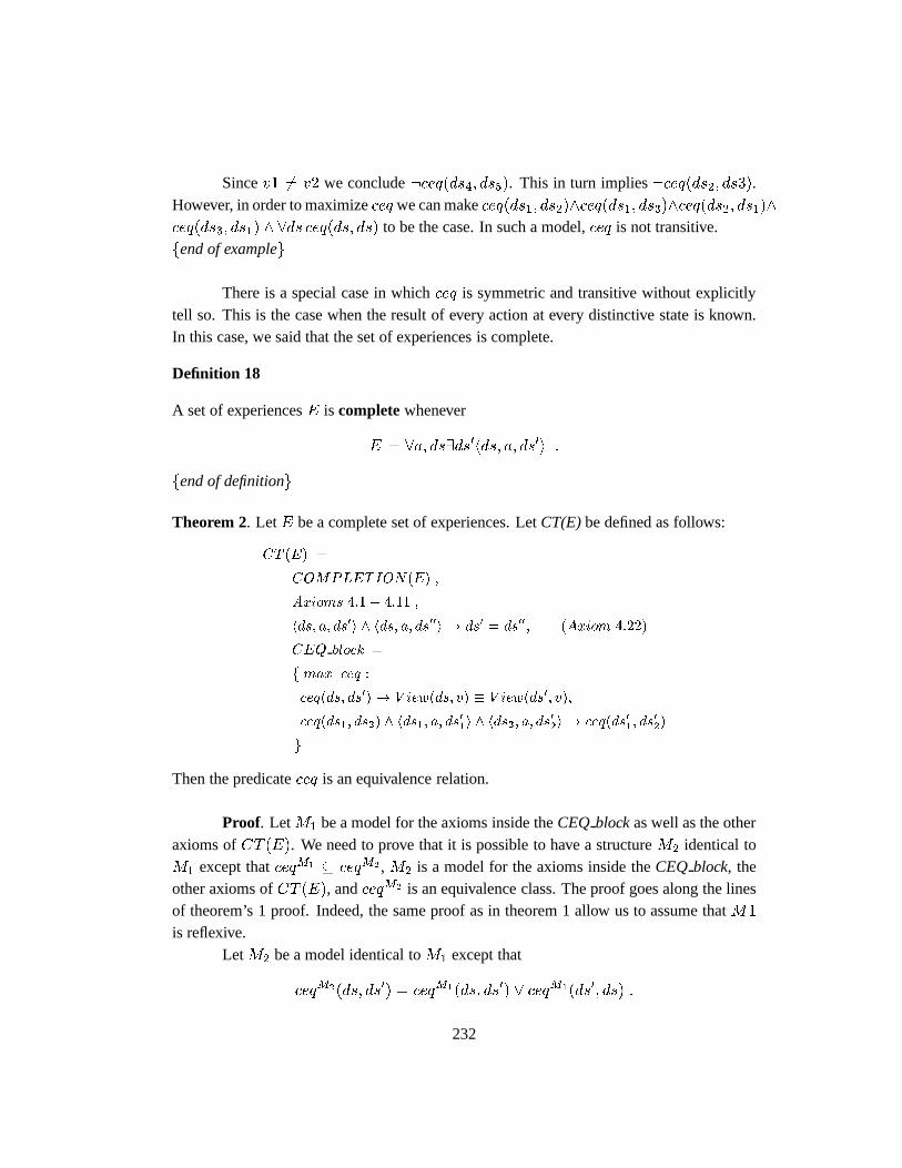
Sincev1 6= v2 we conclude:ceq(ds4; ds5). This in turn implies:ceq(ds2; ds3).However, in order to maximizeceq we can makeceq(ds1; ds2)^ceq(ds1; ds3)^ceq(ds2; ds1)^ceq(ds3; ds1) ^ 8ds ceq(ds; ds) to be the case. In such a model,ceq is not transitive.fend of exampleg

There is a special case in whichceq is symmetric and transitive without explicitlytell so. This is the case when the result of every action at every distinctive state is known.In this case, we said that the set of experiences is complete.

Definition 18

A set of experiencesE is completewhenever

E j= 8a; ds9ds0hds; a; ds0i :

fend of definitiong

Theorem 2. LetE be a complete set of experiences. LetCT(E)be defined as follows:

CT (E) =

COMPLETION(E) ;

Axioms 4:1� 4:11 ;

hds; a; ds0i ^ hds; a; ds00i ! ds0 = ds00; (Axiom 4:22)

CEQ block =

f max ceq :

ceq(ds; ds0)! V iew(ds; v) � V iew(ds0; v);

ceq(ds1; ds2) ^ hds1; a; ds0

1i ^ hds2; a; ds0

2i ! ceq(ds01; ds0

2)

g

Then the predicateceq is an equivalence relation.

Proof. LetM1 be a model for the axioms inside theCEQ blockas well as the otheraxioms ofCT (E). We need to prove that it is possible to have a structureM2 identical toM1 except thatceqM1 � ceqM2 , M2 is a model for the axioms inside theCEQ block, theother axioms ofCT (E), andceqM2 is an equivalence class. The proof goes along the linesof theorem’s 1 proof. Indeed, the same proof as in theorem 1 allow us to assume thatM1

is reflexive.LetM2 be a model identical toM1 except that

ceqM2(ds; ds0) = ceqM1(ds; ds0) _ ceqM1(ds0; ds) :

232

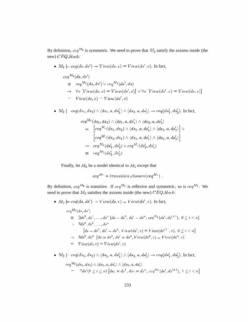
By definition,ceqM2 is symmetric. We need to prove thatM2 satisfy the axioms inside (thenew)CEQ block:

� M2 j= ceq(ds; ds0)! V iew(ds; v) � V iew(ds0; v). In fact,

ceqM2(ds; ds0)

� ceqM1(ds; ds0) _ ceqM1(ds0; ds)

! 8v�V iew(ds; v) � V iew(ds0; v)

�_ 8v

�V iew(ds0; v) � V iew(ds; v)

�� V iew(ds; v) � V iew(ds0; v)

� M2 j= ceq(ds1; ds2) ^ hds1; a; ds01i ^ hds2; a; ds

02i ! ceq(ds01; ds

02). In fact,

ceqM2(ds1; ds2) ^ hds1; a; ds01i ^ hds2; a; ds

02i

�hceqM1(ds1; ds2) ^ hds1; a; ds

01i ^ hds2; a; ds

02ii_h

ceqM1(ds2; ds1) ^ hds1; a; ds01i ^ hds2; a; ds

02ii

! ceqM1(ds01; ds02) _ ceq

M1(ds02; ds01)

� ceqM2(ds01; ds02)

Finally, letM2 be a model identical toM1 except that

ceqM2 = transitive closure(ceqM1) :

By definition, ceqM2 is transitive. IfceqM1 is reflexive and symmetric, so isceqM2 . Weneed to prove thatM2 satisfies the axioms inside (the new)CEQ block:

� M2 j= ceq(ds; ds0)! V iew(ds; v) � V iew(ds0; v). In fact,

ceqM2(ds; ds0)

� 9ds0; ds1; : : : ; dsn�ds = ds0; ds0 = dsn; ceqM1(dsi; dsi+1); 0 � i < n

�! 9ds0; ds1; : : : ; dsn�

ds = ds0; ds0 = dsn; V iew(dsi; v) � V iew(dsi+1; v); 0 � i < n�

! 9ds0; dsn�ds = ds0; ds0 = dsn; V iew(ds0; v) � V iew(dsn; v)

�� V iew(ds; v) � V iew(ds0; v)

� M2 j= ceq(ds1; ds2) ^ hds1; a; ds01i ^ hds2; a; ds

02i ! ceq(ds01; ds

02). In fact,

ceqM2(ds1; ds2) ^ hds1; a; ds0

1i ^ hds2; a; ds0

2i

� 9dsi(1 � i � n)�ds1 = ds1; ds2 = dsn; ceqM1(dsi; dsi+1); 1 � i < n

�233

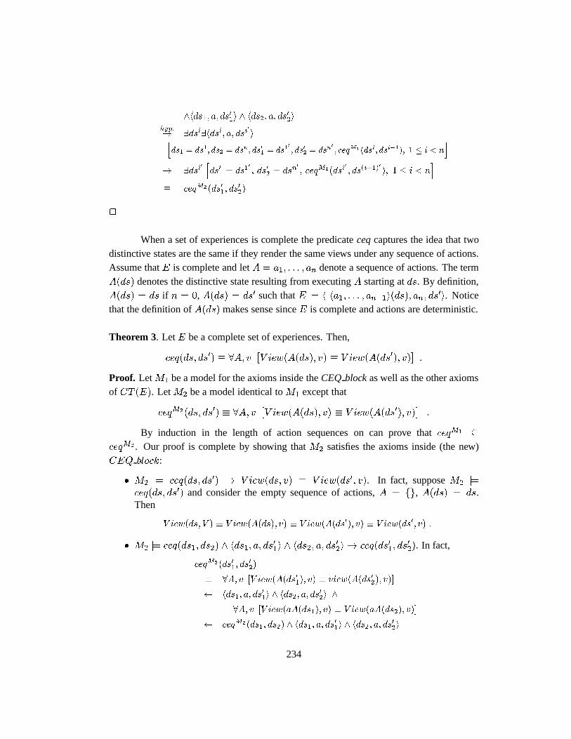
^hds1; a; ds0

1i ^ hds2; a; ds0

2ihyp:! 9dsi9hdsi; a; dsi

0

ihds1 = ds1; ds2 = dsn; ds01 = ds1

0

; ds02 = dsn0

; ceqM1(dsi; dsi+1); 1 � i < n

i! 9dsi

0

hds01 = ds1

0

; ds02 = dsn0

; ceqM1(dsi0

; ds(i+1)0

); 1 � i < ni

� ceqM2(ds01; ds0

2)

2

When a set of experiences is complete the predicateceqcaptures the idea that twodistinctive states are the same if they render the same views under any sequence of actions.Assume thatE is complete and letA = a1; : : : ; an denote a sequence of actions. The termA(ds) denotes the distinctive state resulting from executingA starting atds. By definition,A(ds) = ds if n = 0, A(ds) = ds0 such thatE j= h ha1; : : : ; an�1i(ds); an; ds0i. Noticethat the definition ofA(ds) makes sense sinceE is complete and actions are deterministic.

Theorem 3. LetE be a complete set of experiences. Then,

ceq(ds; ds0) � 8A; v�V iew(A(ds); v) � V iew(A(ds0); v)

�:

Proof. LetM1 be a model for the axioms inside theCEQ blockas well as the other axiomsof CT (E). LetM2 be a model identical toM1 except that

ceqM2(ds; ds0) � 8A; v�V iew(A(ds); v) � V iew(A(ds0); v)

�:

By induction in the length of action sequences on can prove thatceqM1 �

ceqM2 . Our proof is complete by showing thatM2 satisfies the axioms inside (the new)CEQ block:

� M2 j= ceq(ds; ds0) ! V iew(ds; v) � V iew(ds0; v). In fact, supposeM2 j=ceq(ds; ds0) and consider the empty sequence of actions,A = fg, A(ds) = ds.Then

V iew(ds; V ) � V iew(A(ds); v) � V iew(A(ds0); v) � V iew(ds0; v) :

� M2 j= ceq(ds1; ds2) ^ hds1; a; ds01i ^ hds2; a; ds

02i ! ceq(ds01; ds

02). In fact,

ceqM2(ds01; ds0

2)

� 8A; v [V iew(A(ds01); v) � view(A(ds02); v)]

hds1; a; ds0

1i ^ hds2; a; ds0

2i ^

8A; v [V iew(aA(ds1); v) � V iew(aA(ds2); v)]

ceqM2(ds1; ds2) ^ hds1; a; ds0

1i ^ hds2; a; ds0

2i

234

2

235

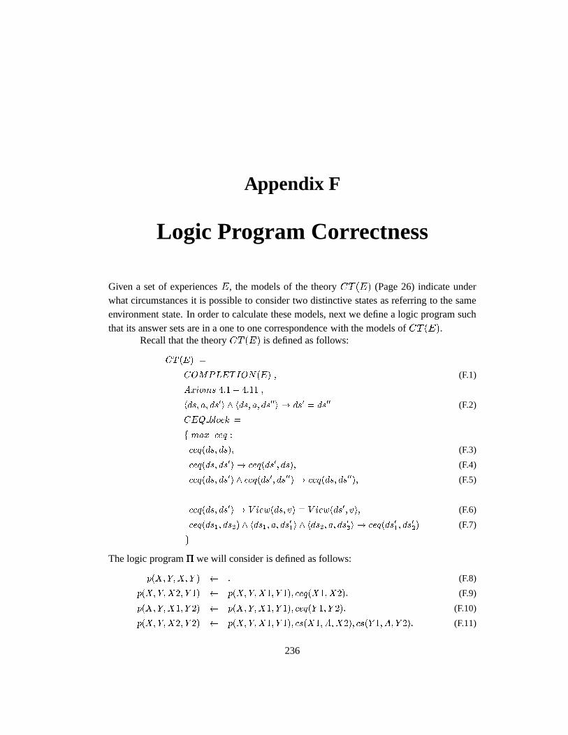
Appendix F

Logic Program Correctness

Given a set of experiencesE, the models of the theoryCT (E) (Page 26) indicate underwhat circumstances it is possible to consider two distinctive states as referring to the sameenvironment state. In order to calculate these models, next we define a logic program suchthat its answer sets are in a one to one correspondence with the models ofCT (E).

Recall that the theoryCT (E) is defined as follows:

CT (E) =

COMPLETION(E) ; (F.1)

Axioms 4:1� 4:11 ;

hds; a; ds0i ^ hds; a; ds00i ! ds0 = ds00 (F.2)

CEQ block =

f max ceq :

ceq(ds; ds); (F.3)

ceq(ds; ds0)! ceq(ds0; ds); (F.4)

ceq(ds; ds0) ^ ceq(ds0; ds00)! ceq(ds; ds00); (F.5)

ceq(ds; ds0)! V iew(ds; v) � V iew(ds0; v); (F.6)

ceq(ds1; ds2) ^ hds1; a; ds0

1i ^ hds2; a; ds0

2i ! ceq(ds01; ds0

2) (F.7)

g

The logic program� we will consider is defined as follows:

p(X;Y;X; Y ) : (F.8)

p(X;Y;X2; Y 1) p(X;Y;X1; Y 1); ceq(X1; X2): (F.9)

p(X;Y;X1; Y 2) p(X;Y;X1; Y 1); ceq(Y 1; Y 2): (F.10)

p(X;Y;X2; Y 2) p(X;Y;X1; Y 1); cs(X1; A;X2); cs(Y 1; A; Y 2): (F.11)

236

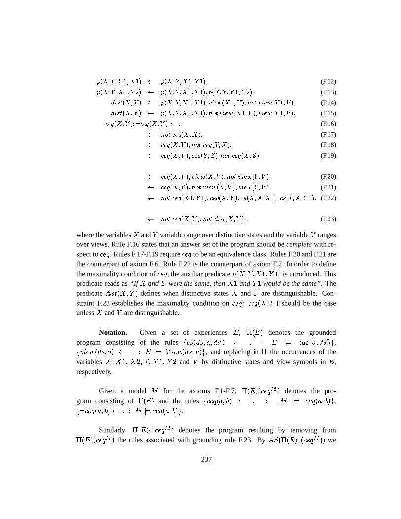
p(X;Y; Y 1; X1) p(X;Y;X1; Y 1): (F.12)

p(X;Y;X1; Y 2) p(X;Y;X1; Y 1); p(X;Y; Y 1; Y 2): (F.13)

dist(X;Y ) p(X;Y;X1; Y 1); view(X1; V ); not view(Y 1; V ): (F.14)

dist(X;Y ) p(X;Y;X1; Y 1); not view(X1; V ); view(Y 1; V ): (F.15)

ceq(X;Y );:ceq(X;Y ) : (F.16)

not ceq(X;X): (F.17)

ceq(X;Y ); not ceq(Y;X): (F.18)

ceq(X;Y ); ceq(Y; Z); not ceq(X;Z): (F.19)

ceq(X;Y ); view(X;V ); not view(Y; V ): (F.20)

ceq(X;Y ); not view(X;V ); view(Y; V ): (F.21)

not ceq(X1; Y 1); ceq(X;Y ); cs(X;A;X1); cs(Y;A; Y 1): (F.22)

not ceq(X;Y ); not dist(X;Y ): (F.23)

where the variablesX andY variable range over distinctive states and the variableV rangesover views. Rule F.16 states that an answer set of the program should becompletewith re-spect toceq. Rules F.17-F.19 requireceq to be an equivalence class. Rules F.20 and F.21 arethe counterpart of axiom F.6. Rule F.22 is the counterpart of axiom F.7. In order to definethe maximality condition ofceq, the auxiliar predicatep(X;Y;X1; Y 1) is introduced. Thispredicate reads as“If X andY were the same, thenX1 andY 1 would be the same”. Thepredicatedist(X;Y ) defines when distinctive statesX andY are distinguishable. Con-straint F.23 establishes the maximality condition onceq: ceq(X;Y ) should be the caseunlessX andY are distinguishable.

Notation. Given a set of experiencesE, �(E) denotes the groundedprogram consisting of the rulesfcs(ds; a; ds0) : : E j= hds; a; ds0ig,fview(ds; v) : : E j= V iew(ds; v)g, and replacing in� the occurrences of thevariablesX; X1; X2; Y; Y 1; Y 2 and V by distinctive states and view symbols inE,respectively.

Given a modelM for the axioms F.1-F.7,�(E)(ceqM ) denotes the pro-gram consisting of�(E) and the rulesfceq(a; b) : : M j= ceq(a; b)g,f:ceq(a; b) : : M 6j= ceq(a; b)g.

Similarly, �(E)1(ceqM ) denotes the program resulting by removing from

�(E)(ceqM ) the rules associated with grounding rule F.23. ByAS(�(E)1(ceqM )) we

237

denote the answer set of�(E)1(ceqM ) (see lemma 2, page 239).

We say thatceqM is maximalin M wheneverM is a model forCT (E).1

fend of notationg

Using the notation above we can state our theorem as follows:

Theorem 13 ceqM is maximalin M if and only ifAS(�(E)1(ceqM )) is an answer set for�(E)(ceqM ).

Notice that theorem 13 establishes a one to one correspondence between the an-swer sets of�(E) and the models ofCT (E). Given a modelM for CT (E), ceqM ismaximal in M , and soAS(�(E)1(ceqM )) is an answer set for�(E)(ceqM ), thus, ananswer set for�(E).2 Conversely, given any answer setX for �(E), the modelMdefined such thatM j= E and ceqM = f(ds; ds0) : ceq(ds; ds0) 2 Xg, is such thatAS(�(E)1(ceq

M )) = X.3 Consequently,ceqM is maximalin M , that is,M is a modelfor CT (E).

Proof of theorem 13.(a) SupposeceqM is maximal inM andAS(�(E)1(ceqE)) is not an answer set

for �(E)(ceqM ). SinceAS(�(E)1(ceqM )) is an answer set for�(E)1(ceqM ), thenAS(�(E)1(ceq

M )) does not satisfy constraint F.23.4 Consequently, there exist distinctivestatesX andY such that:

1. ceq(X;Y ) 62 AS(�(E)1(ceqM )), and

2. dist(X;Y ) 62 AS(�(E)1(ceqM )).

Defineceq1M in M such thatM j= ceq1(a; b) wheneverM j= ceq(a; b) or p(X;Y; a; b) 2AS(�(E)1(ceq

M )). Symbolically,

ceq1M (a; b) � ceqM (a; b) _ p(X;Y; a; b) :

By definition,ceqM � ceq1M .5 We are to prove thatceq1M satisfies axioms F.3-F.7, whichwill contradict the fact thatceqM is maximal inM :

1Recall thatceqM denotes the interpretation ofceq in the structureM .2Let X be an answer set for�(E)(ceqM) and considerY � X closed under�(E). Then, in virtue of

F.16,Y is closed underceqM and soX = Y .3Given any program� andX an answer set for�,X is the unique answer set for� [X.4The answer sets of�(E)(ceqM) are those answer sets of�(E)1(ceq

M ) that satisfy constraint F.23.5Sincep(X;Y;X; Y ) 2 AS(�(E)1(ceq

M ))

238

� By lemma 3,ceq1M is an equivalence relation.

� Suppose thatceq1M (ds; ds0) is the case. IfceqM (ds; ds0) is the case, thenM j= V iew(ds; v) � V iew(ds0; v). If p(X;Y; ds; ds0) is the case, thenV iew(ds; v) � V iew(ds0; v) is the case, since otherwisedist(X;Y ) will belongtoAS(�(E)1(ceq)).6

� Suppose thatM j= ceq1(ds1; ds2) ^ hds1; a; ds01i ^ hds2; a; ds

02i. If M j=

ceq(ds1; ds2) is the case, thenM j= ceq(ds01; ds02) is the case. Ifp(X;Y; ds1; ds2)

is the case, by rule F.11,p(X;Y; ds01; ds02) 2 AS(�(E)1(ceq

M )) and soM j=

ceq1(ds01; ds02).

2

(b) Suppose thatAS(�(E)1(ceq)) is an answer set for�(E)(ceqM ) andceqM isnot maximal inM . Then, there existsceq1M , ceqM � ceq1M , ceq1M maximal inM .Moreover, by the if part of this theorem, (a) above,AS(�(E)1(ceq1

M )) is an answer setfor �(E)(ceq1M ). LetX andY be such that:

1. M j= ceq1(X;Y ),

2. M 6j= ceq(X;Y ), and so (Lemma 2)ceq(X;Y ) 62 AS(�(E)1(ceqM )).

SinceAS(�(E)1(ceqM )) satisfies constraint F.23, thendist(X;Y ) 2 AS(�(E)1(ceqM )),

and consequently (rules F.14-F.15) there existX1,Y 1 andV , such that

1. p(X;Y;X1; Y 1) 2 AS(�(E)1(ceqM )),

2. M j= V iew(X1; V ) 6� V iew(Y 1; V ).

SinceceqM � ceq1M , thenp(X;Y;X1; Y 1) 2 AS(�(E)1(ceq1M )) (Lemma 4). Since

ceq(X;Y ) 2 AS(�(E)1(ceq1M )), thenceq(X1; Y 1) 2 AS(�(E)1(ceq1

M )) (Lemma 5)which is a contradiction sinceAS(�(E)1(ceq1M )) satisfies constraints F.20-F.21.

2

Lemma 2 LetM be a model for axioms F.1-F.7. LetceqM be the interpretation ofceq inM .7 Then�(E)1(ceqM ) has a unique answer set which we denote byAS(�(E)1(ceq

M )).Moreover, for any two distinctive statesds and ds0, M j= ceq(ds; ds0) if and only ifceq(ds; ds0) 2 AS(�(E)1(ceq

M )).6This is the case according to rules F.14 and F.15, and the fact thatAS(�(E)1(ceq)) is the answer set for

�(E)1(ceq).7The interpretation ofceq in M is not necessarily maximal.

239

Proof. Let�(E)2(ceqM ) denote the program resulting of removing from�(E)1(ceqM )

those constraints resulting from grounding rules F.17-F.22. The answer sets of�(E)1(ceqM )

are those answer sets of�(E)2(ceqM ) satisfying constraints F.17-F.22. We are to prove that

�(E)2(ceqM ) has a unique answer set satisfying constraints F.8-F.15.

Let Facts denote the union of the setsfcs(ds; a; ds0) : : E j= hds; a; ds0ig,fview(ds; v) : : E j= V iew(ds; v)g, fceq(a; b) : : M j= ceq(a; b)g, andf:ceq(a; b) : : M 6j= ceq(a; b)g. Any answer set of�(E)2(ceqM ) containsFacts.Let X andY denote two possible answer sets for�(E)2(ceq

M ). Then the reduct ofXandY are the same,�(E)2(ceqM )X = �(E)2(ceq

M )Y , since bothX andY agree onthe literals of the formview(ds; v).8 Consequently,�(E)2(ceqM ) has at most one answerset. In fact,Cn(�(E)2(ceqM )Facts) is such answer set.9 In particular, ceq(ds; ds0) 2Cn(�(E)2(ceq

M )Facts) iff ceq(ds; ds0) 2 Facts iff M j= ceq(ds; ds0).Finally, sinceceqM satisfies axioms F.3-F.7 thenCn(�(E)2(ceqM )Facts) satisfies

constraints F.17-F.22, thus, it is an answer set for�(E)1(ceqM ). 2

Lemma 3 LetM be a model for axioms F.1-F.7. LetceqM be the interpretation ofceq inM , and letAS(�(E)1(ceqM )) be the answer set for�(E)1(ceqM ). LetX andY be twoarbitrary distinctive state symbols. Letceq1M inM be such thatM j= ceq1(a; b) wheneverM j= ceq(a; b) or p(X;Y; a; b) 2 AS(�(E)1(ceqM )). Symbolically,

ceq1M (a; b) � ceqM (a; b) _ p(X;Y; a; b) :

Then,ceq1M is an equivalence relation.

Proof.

� ceq1 is reflexive. Indeed,

ceq1M (ds; ds) � ceqM (ds; ds) _ p(X;Y; ds; ds)F:3� ceqM (ds; ds) :

� ceq1 is symmetric. Indeed,

ceq1M (ds; ds0) � ceqM (ds; ds0) _ p(X;Y; ds; ds0)F:4� ceqM (ds0; ds) _ p(X;Y; ds; ds0)F:12� ceqM (ds0; ds) _ p(X;Y; ds0; ds)

� ceq1M (ds1; ds)

8Notice thatview(ds; ds0) 2 X iff view(ds; ds0) 2 Facts.9Cn(�) denotes the set of consequences of a logic program without negation as failure.

240

� ceq1 is transitive. Indeed,

ceq1M (ds; ds0) ^ ceq1M (ds0; ds00)

� fceqM (ds; ds0) _ p(X;Y; ds; ds0)g ^ fceqM (ds0; ds00) _ p(X;Y; ds0; ds00)g

� fceqM (ds; ds0) ^ ceqM (ds0; ds00)g _ fceqM (ds; ds0) ^ p(X;Y; ds0; ds00)g _

fp(X;Y; ds; ds0) ^ ceqM (ds0; ds00)g _ fp(X;Y; ds; ds0) ^ p(X;Y; ds0; ds00)gF:5;F:13! ceqM (ds; ds00) _ fceqM(ds; ds0) ^ p(X;Y; ds0; ds00)g _

fp(X;Y; ds; ds0) ^ ceqM (ds0; ds00)g _ p(X;Y; ds; ds00)F:9; F:10! ceqM (ds; ds00) _ p(X;Y; ds; ds00) _ p(X;Y; ds; ds00) _ p(X;Y; ds; ds00)

� ceqM (ds; ds00) _ p(X;Y; ds; ds00)

� ceq1M (ds; ds00)

2

Lemma 4 LetM be a model for axioms F.1-F.7, and letceqM , ceq1M , ceqM � ceq1M ,be two relations such that both satisfy axioms F.3-F.7. Then,AS(�(E)1(ceq

M )) �

AS(�(E)1(ceq1M )).

Proof. Let �(E)2(ceqM ) denote the program resulting of removing from�(E)1(ceq

M ) those constraints resulting from grounding rules F.17-F.22. LetFacts de-note the union of the setsfcs(ds; a; ds0) : : E j= hds; a; ds0ig, fview(ds; v) : : E j= view(ds; v)g, fceq(a; b) : : M j= ceq(a; b)g, andf:ceq(a; b) : :

M 6j= ceq(a; b)g. DefineFacts1 in the same way asFacts but usingceq1 insteadof ceq. Since,ceqM � ceq1M , it is the case thatFacts � Fact1 and consequently�(E)2(ceq

M ) � �(E)2(ceq1M ).

Since, Facts and Facts1 agree on literals of the formview(ds; v), itfollows that �(E)2(ceq

M )Facts � �(E)2(ceq1M )Facts1. It follows then that

Cn(�(E)2(ceqM )Facts) � Cn(�(E)2(ceq

M )Facts1) � Cn(�(E)2(ceq1M )Facts1).

In lemma 2 we prove thatAS(�(E)1(ceqM )) = Cn(�(E)2(ceqM )Facts) and

AS(�(E)1(ceq1M )) = Cn(�(E)2(ceq

M )Facts1). Therefore,AS(�(E)1(ceqM )) �

AS(�(E)1(ceq1M )).

2

Lemma 5 Let M be a model for axioms F.1-F.7. IfceqM (ds; ds0) andp(ds; ds0; ds1; ds10) 2 AS(�(E)1(ceq

M )), thenceqM (ds1; ds10).

241

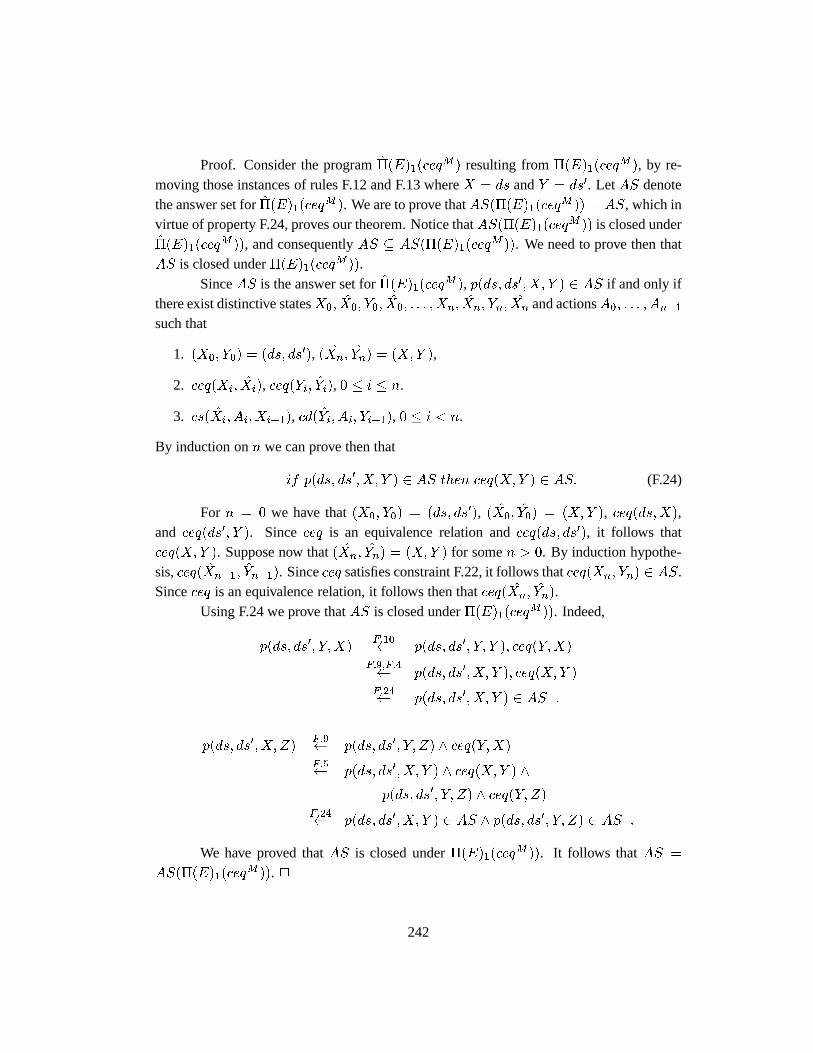
Proof. Consider the program�(E)1(ceqM ) resulting from�(E)1(ceqM ), by re-

moving those instances of rules F.12 and F.13 whereX = ds andY = ds0. LetAS denotethe answer set for�(E)1(ceqM ). We are to prove thatAS(�(E)1(ceqM )) = AS, which invirtue of property F.24, proves our theorem. Notice thatAS(�(E)1(ceq

M )) is closed under�(E)1(ceq

M )), and consequentlyAS � AS(�(E)1(ceqM )). We need to prove then that

AS is closed under�(E)1(ceqM )).SinceAS is the answer set for�(E)1(ceqM ), p(ds; ds0;X; Y ) 2 AS if and only if

there exist distinctive statesX0; X0; Y0; X0; : : : ;Xn; Xn; Yn; Xn and actionsA0; : : : ; An�1

such that

1. (X0; Y0) = (ds; ds0), (Xn; Yn) = (X;Y ),

2. ceq(Xi; Xi), ceq(Yi; Yi), 0 � i � n.

3. cs(Xi; Ai;Xi+1), cd(Yi; Ai; Yi+1), 0 � i < n.

By induction onn we can prove then that

if p(ds; ds0;X; Y ) 2 AS then ceq(X;Y ) 2 AS: (F.24)

For n = 0 we have that(X0; Y0) = (ds; ds0), (X0; Y0) = (X;Y ), ceq(ds;X),and ceq(ds0; Y ). Sinceceq is an equivalence relation andceq(ds; ds0), it follows thatceq(X;Y ). Suppose now that(Xn; Yn) = (X;Y ) for somen > 0. By induction hypothe-sis,ceq(Xn�1; Yn�1). Sinceceq satisfies constraint F.22, it follows thatceq(Xn; Yn) 2 AS.Sinceceq is an equivalence relation, it follows then thatceq(Xn; Yn).

Using F.24 we prove thatAS is closed under�(E)1(ceqM )). Indeed,

p(ds; ds0; Y;X)F:10 p(ds; ds0; Y; Y ); ceq(Y;X)

F:9;F:4 p(ds; ds0;X; Y ); ceq(X;Y )F:24 p(ds; ds0;X; Y ) 2 AS :

p(ds; ds0;X; Z)F:9 p(ds; ds0; Y; Z) ^ ceq(Y;X)F:5 p(ds; ds0;X; Y ) ^ ceq(X;Y ) ^

p(ds; ds0; Y; Z) ^ ceq(Y;Z)F:24 p(ds; ds0;X; Y ) 2 AS ^ p(ds; ds0; Y; Z) 2 AS :

We have proved thatAS is closed under�(E)1(ceqM )). It follows thatAS =

AS(�(E)1(ceqM )). 2

242

Appendix G

MERCATOR’s Ontology andSemantics

MERCATOR [Davis, 1993] usesclumps , regions, polygons, joints, edges, verticesandPCOs.1 The basic elements of the representation are straight line segments. Theboundary of an object is represented by a set ofedgesconnectingvertices. Boundary edgesare labeled with directions specifying the direction counter-clockwise around the object.Such a directed edge is called abound. The interior of an object is represented bypolygons.A complete shape description, consisting of a set of bounds and a set of polygons, is calleda region.

Local dimensions are recorded in terms of the lengths and orientations of edgesconnecting the vertices. Lengths and orientations are not specified precisely. Rather, therange in which they lie is specified. The measure of the inaccuracy of a region is itsgrain-size, which is an upper bound on the distance from any point in the region to a point in theobject. The smaller the grain-size, the better the approximation. Also, every bound in aregion has a grain-size which, roughly speaking, is an upper bound on the distance from thebound to the corresponding part of the boundary.

The overall representation of an object is called aclump; it contains all the regionsof the object, plus descriptions of the properties of the object, and the relations between theregions. A map is hierarchically arranged by containment. Clumps point to their immediatecontainers and contents.

1PCO stands for Partial Circular Ordering.

243

Different regions for a clump can be related to one another in three ways. Firstly,different regions may share one or more edges. Secondly, vertices of different edges may beconnected by edges or joints. Thirdly, the order of the external vertices around the bound-ary is recorded inpartial circular ordering (PCO). Given two vertices, aPCO expresseswhether they are in clockwise order, counter clockwise order, or unordered.

An objectO is a closed, connected subset ofR2 (the real plane) with a boundaryconsisting of a finite number of disjoint simple closed curves. Apropertyis a function fromobjects to arbitrary sets. A MERCATOR map describes a set of objects with properties.

Three functions relate the MERCATOR map to the real world: REAL, COOR, andCOVER. REAL maps clumps onto objects. REAL preserves containment (i.e. if CL1contains CL2, then REAL(CL1) must contain REAL(CL2)) and it takes clumps with statedproperties onto objects with these properties. COOR takes vertices of the map into pointsin the plane (even if a pointg represents an object with some extent, COOR (g) is a singlepoint in the plane). COOR is extended in the natural way to take edges into line segments,joints into pairs of line segments, polygons of the map into planar polygons, and regionsinto unions of polygons. COOR has to satisfy the following conditions:

1. For each edgee,COOR(e) has to have length and orientation within the fuzz rangeswhich the map specifies fore. Likewise for joints.

2. For each polygonP in the map,COOR(P ) must define a polygon in the plane.

3. For each regionR, every point inCOOR(R) must be no further than the grain-sizeof the interior ofR from the object represented byR.

COVER is a family of functions. COOR, as stated, maps directed edges onto linesegments in the plane. However, we must relate boundary edges to the part of the objectboundary that they represent. Therefore, for each directed edgeb in the boundary of a re-gion, we define a continuous functionCOV ERb fromCOOR(b) into the object boundary.COV ERb must satisfy the following conditions:

1. For allx 2 COOR(b), the distance fromx to COV ERb(x) must be less than thegrain-size ofb.

2. If b andc are directed edges from the shell of regionR which meet at a vertexv, andv is a real bound ofR, thenCOVERb(COOR(v)) = COORc(COOR(v)).

3. The real vertices of a clump map into the boundary of the corresponding object so asto satisfy the PCOs of the clump.

244

The MERCATOR map is valid if it is possible to define REAL, COOR, and COVER so asto satisfy all these conditions.

245

Bibliography

[Angluin, 1978] Dana Angluin. On the complexity of minimum inference of regular sets.Information and Control, 39:337–350, 1978.

[Angluin, 1987] Dana Angluin. Learning regular sets from queries and counterexamples.Information and Computation, 75:87–106, 1987.

[Anousaki and Kyriakopoulos, 1999] G.C. Anousaki and T. Kyriakopoulos. Simultaneouslocalization and map building for mobile robot navigation.IEEE Robotics & AutomationMagazine, pages 42–53, 1999.

[Aurenhammer, 1991] F. Aurenhammer. Voronoi diagrams– a survey of fundamental geo-metric structure.ACM Computing Surveys, 23:345–405, 1991.

[Bacchuset al., 1999] F. Bacchus, J. Halpern, and H. Levesque. Reasoning about noisysensors and effectors in the situational calculus.Artificial Intelligence, 111:171–208,1999.

[Baral and Gelfond, 1997] Chitta Baral and Michael Gelfond. Reasoning about effects ofconcurrent actions.Journal of Logic Programming, 31(1-3):85–117, 1997.

[Baral and Gelfond, 1999] Chitta Baral and Michael Gelfond. Reasoning agents in dy-namic domains. In Jack Minker, editor,Workshop on Logic-Based Artificial Intelligence,Washington, DC, June 14–16, 1999, College Park, Maryland, 1999. Computer ScienceDepartment, University of Maryland.

[Basyeet al., 1995] K. Basye, T. Dean, and L.P. Kaelbling. Learning dynamics: Systemidentification for perceptually challenged agents.Artificial Intelligence, 72(1):139–171,1995.

[Beardon, 1979] A. F. Beardon.Complex Analysis. John Weley & Sons, New York, 1979.

246

[Bickhard M., 1995] Terveen L. Bickhard M.Foundational issues in Artificial Intelligenceand Cognitive Science: Impasse and Solution.North Holland, Elsevier Science B.V.,first edition, 1995.

[Borensteinet al., 1996] J. Borenstein, H.R. Everett, and L. Feng.Navigating mobilerobots: systems and techniques. A K Peters, Wellesley, Massachusetts, 1996.

[Borestein and Koren, 1991] J. Borestein and Y. Koren. The vector field histogram -fast obstacle-avoidance for mobile robots.IEEE Journal of Robotics and Automation,7(3):278–288, 1991.

[Borg and Groenen, 1997] Ingwer Borg and Patrick Groenen.Modern multidimensionalscaling: theory and applications. Springer, New York, 1997.

[Choset and Nagatani, 2001] H. Choset and K. Nagatani. Topological simultaneous local-ization and mapping (SLAM): toward exact localization without explicit localization.IEEE Trans. on Robotics and Automation, 17(2):125–137, April 2001.

[Chosetet al., 1997] H. Choset, I. Konuksven, and A. Rizzi. Sensor based planning: Acontrol law for generating the generalized voronoi diagram.IEEE International Confer-ence in Autonomous Robots, 1997.

[Cormenet al., 1993] Thomas H. Cormen, Charles E. Leiserson, and Ronald L. Rivest.Introduction to Algorithms. The MIT press, Cambridge, Massachusetts, 1993.

[Crawford and Kuipers, 1991] J. Crawford and B. Kuipers. Algernon: a tractable systemfor knowledge representation.SIGART Bulleting, 2(3):35–44, 1991.

[Davis, 1993] E. Davis. The Mercator representation of spatial knowledge. InAAAI-93,1993.

[De Giacomoet al., 1997] G. De Giacomo, Y. Lesperance, and H. Levesque. Reasoningabout concurrent execution, prioritized interrupts, and exogenous actions in the situationcalculus. InIJCAI 97, Nagoya, pages 1221–1226, 1997.

[Duboi and Prade, 1988] D. Duboi and H. Prade. Representation and combination of un-certainty with belief functions and possibility measures.Computational Intelligence,4:244–264, 1988.

[Duckett and Nehmzow, 2000] Tom Duckett and Ulrich Nehmzow. Performance compari-son of landmark recognition systems for navigating mobile robots. InAAA-I 2000, pages826–831, July-August 2000.

247

[Dudeket al., 1991] Gregory Dudek, Jenkin Michael, Evangelos Milios, and DavidWilkes. Robotic exploration as graph construction.IEEE Trans. on Robotics and Au-tomation, 7(6):859–865, 1991.

[Durrant-Whyte, 1987] H. F. Durrant-Whyte. Consistent integration and propagation ofdisparate sensor observations.The International Journal of Robotics Research, 6(3):3–24, 1987.

[Durrant-Whyte, 1988a] H. F. Durrant-Whyte.Integration, coordination and control ofmultisensor robot systems. Kluwer Academic Publishers, Boston, 1988.

[Durrant-Whyte, 1988b] H. F. Durrant-Whyte. Uncertain geometry in robotics.IEEE Jour-nal of Robotics and Automation, 5(6):23–31, 1988.

[Elfes, 1987] Alberto Elfes. Sonar-based real-world mapping and navigation.IEEE Jour-nal of Robotics and Automation, RA3(3):249–265, 1987.

[Engelson and McDermott, 1992a] Sean P. Engelson and Drew V. McDermott. Maps con-sidered as adaptive planning resources. InAAAI Fall Symposium on Applications of AIto Real-World Autonomous Mobile Robots, Working Notes, Cambridge, MA, October1992.

[Engelson and McDermott, 1992b] S.P. Engelson and D.V. McDermott. Error correctionin mobile robot map learning. Inthe IEEE International Conference on Robotics andAutomation, pages 2555–2560, 1992.

[Fernandez and Gonzalez, 1997] Juan Fernandez and Javier Gonzalez. A general worldrepresentation for mobile robot operations. InSeventh conference of the Spanish as-sociation for artificial intelligence (CAEPIA-97), 1997.

[Fernandez and Gonzalez, 1998] Juan Fernandez and Javier Gonzalez. Hierarchical graphsearch for mobile robot planning. InIEEE international conference on Robotics andAutomation, 1998.

[Fernandez, 2000] Juan Fernandez.Modeling and Generation of Multiple Abstractions forRepresenting Large-Scale Space. An Application to Mobile Robots.PhD thesis, Univer-sity of Malaga, Spain, 2000.

[Fikes and Nilsson, 1971] R. Fikes and N. Nilsson. Strips: A new approach to the applica-tion of theorem proving to problem solving.Artificial Intelligence, 2:189–208, 1971.

248

[Firby, 1994] R. James Firby. Task networks for controlling continuous processes. In Kris-tian Hammond, editor,Second International Conference on AI Planning Systems, pages49–54. AAAI Press, 1994.

[Franzet al., 1998] M. Franz, B. Sch�olkopf, H. Mallot, and B�ulthoff. Learning view graphsfor robot navigation.Autonomous robots, 5:111–125, 1998.

[Freksa, 1992] C. Freksa. Using orientation information for qualitative spatial reasoning.Theories and Models of Spatio-Temporal Reasoning in Geographic Space, 639:162–178,1992.

[Gat, 1996] Erann Gat. ESL: A language for supporting robust plan execution in embeddedautonomous agents. InPlan Execution: Problems and Issues: Papers from the 1996AAAI Fall Symposium, pages 59–64. AAAI Press, Menlo Park, California, 1996.

[Gelb, 1974] A. Gelb.Applied Optimal Estimation. MIT Press, Cambridge, MA, 1974.

[Gelfond and Lifschitz, 1991] M. Gelfond and V. Lifschitz. Classical negation in logic pro-grams and disjunctive databases.New Generation Computing, 9:365–385, 1991.

[Gelfond and Lifschitz, 1998] M. Gelfond and V. Lifschitz. Action Languages.Link�opingelectronic articles in computer and information sciences, 3(16), 1998.

[Gershenfeld, 1999] Neil Gershenfeld.The Nature of Mathematical Modeling. CambridgeUniversity Press, 1999.

[Giunchiglia and Lifschitz, 1998] E. Giunchiglia and V. Lifschitz. An action laguage basedon causal explanation: preliminary report. InAAAI-98, pages 623–630, 1998.

[Gold, 1978] E. Mark Gold. Complexity of automaton identification from given sets.In-formation and Control, 37:302–320, 1978.

[Gonzalez and Woods, 1992] Rafael C. Gonzalez and Richard E. Woods.Digital ImageProcessing. Addison-Wesley Publishing Company, 1992.

[Gopal and Smith, 1990] S. Gopal and T.R. Smith. Human way-finding in an urban envi-ronment: a performance analysis of a computational process model.Environment andPlanning, 22:169–191, 1990.

[Gopalet al., 1989] S. Gopal, R. L. Klatzky, and T. R. Smith. Navigator: a psychologicallybased model of environmental learning through navigation.Journal of EnvironmentalPsychology, 9:309–331, 1989.

249

[Green, 1969] C. Green. Applications of theorem proving to problem solving. InIJCAI-69,pages 219–240, 1969.

[Hernandez, 1994] D. Hernandez.Qualitative Representation of Spatial Knowledge. Num-ber 804 in Lecture Notes in Computer Science. Springer-Verlag, 1994.

[J., 1991] Levenick J. NAPS: A connectionist implementation of cognitive maps.Connec-tion Science, 3:107–126, 1991.

[Kay et al., 1999] Herbert Kay, Bernard Rinner, and Benjamin Kuipers. Semi-quantitavivesystem identification. Technical Report AI99-279, Computer Science Department, Uni-versity of Texas at Austin, March 1999.

[Koenig and Simmons, 1996] S. Koenig and Reid Simmons. Passive distance learning forrobot navigation. InProceedings ofthe Thirteenth International Conference on MachineLearning (ICML), pages 266 – 274, 1996.

[Koening and Simmons, 1998] S. Koening and R.G. Simmons. XAVIER: A robot navi-gation architecture based on partially observable markov decision process models. InArtificial Intelligence and Mobile Robots, pages 91–122. MIT press, 1998.

[Konoligeet al., 1995] K. Konolige, A. Saffiotti, and E. Ruspini. A multivalued logic ap-proach to integrating planning and control.Artificial Intelligence, 76:481–526, 1995.

[Kortenkampet al., 1995] D. Kortenkamp, E. Chown, and S. Kaplan. Prototypes, loca-tions, and associative networks (PLAN): towards a unified theory of cognitive mapping.Cognitive Science, 19:1–51, 1995.

[Kortenkampet al., 1998] D. Kortenkamp, R.P. Bonasso, and R. Murphy.Artificial Intelli-gence and Mobile Robots. AAAI Press, 1998.

[Kuipers and Byun, 1988] B. Kuipers and Y. T. Byun. A robust qualitative method for spa-tial learning in unknown environments. In Morgan Kaufmann, editor,AAAI-88, 1988.

[Kuipers and Byun, 1991] B. Kuipers and Y. T. Byun. A robot exploration and mappingstrategy based on semantic hierarchy of spatial representations.Journal of Robotics andAutonomous Systems, 8:47–63, 1991.

[Kuipers and Levitt, 1988] Benjamin. Kuipers and T. Levitt. Navigation and mapping inlarge-scale space.AI Magazine, 9(2):25–43, 1988.

250

[Kuiperset al., 1993] B. Kuipers, R. Froom, W.Y. Lee, and D. Pierce. The semantic hier-archy in robot learning. In J. Connell and S. Mahadevan, editors,Robot Learning, pages141–170. Kulwer Academic Publishers, 1993.

[Kuipers, 1978] Benjamin Kuipers. Modeling spatial knowledge.Cognitive Science,2:129–153, 1978.

[Kuipers, 1996] Benjamin Kuipers. A hierarchy of qualitative representations for space. InWorking papers of the Tenth International Workshop on Qualitative Reasoning aboutPhysical Systems (QR-96). AAAI Press, 1996.

[Kuipers, 2000] Benjamin Kuipers. The spatial semantic hierarchy.Artificial IntelligenceJournal, 119:191–233, 2000.

[Kuo, 1987] B. C. Kuo.Automatic Control Systems. Prentice-Hall, Inc., fifth edition, 1987.

[Lee, 1996] W. Y. Lee.Spatial Semantic Hierarchy for a Physical Mobile Robot. PhD the-sis, The University of Texas at Austin, 1996.

[Leiser and Zilbershatz, 1989] David Leiser and Avishai Zilbershatz. THE TRAVELLER:a computational model of spatial network learning.Environment and Behavior,21(4):435–463, 1989.

[Lesperanceet al., 1994] Y. Lesperance, H. Levesque, F. Lin, D. Marcu, R. Reiter, andR. Scherl. A logical approach to high level robot programming: a progress report. InKuipers B., editor,Control of the physical world by intelligent systems: papers from the1994 AAAI fall symposium, pages 79–85, 1994.

[Levitt and Lawton, 1990] T. S. Levitt and D. T. Lawton. Qualitative navigation for mobilerobots.Artificial intelligence, 44(3):305–360, 1990.

[Lifschitz, 1994] Vladimir Lifschitz. Circumscription. InHandbook of Logic in ArtificialIntelligence and Logic Programming, volume 3, pages 297–352. Oxford UniversityPress, 1994.

[Lifschitz, 1995] Vladimir Lifschitz. Nested abnormality theories.Artificial Intelligence,(74):351–365, 1995.

[Lifschitz, 1999] V. Lifschitz. Answer set planning.International Conference on LogicProgramming, 9:23–37, 1999.

[Lobo et al., 1997] J. Lobo, S. Taylor, and G. Mendez. Adding knowledge to the actiondescription language A. InAAAI-97, pages 454–459, 1997.

251

[Mallory et al., 1996] R. Mallory, B. Porter, and B. Kuipers. Comprehending complex be-havior graphs through abstraction. InWorking papers of the tenth international workshopon qualitative reasoning about physical systems (QR-96). AAAI press, 1996.

[Mallot and Gillner, 2000] H. A. Mallot and S. Gillner. Route navigating without placerecognition: What is recognized in recognition-triggered responses?Perception, 29:43–55, 2000.

[Markman, 1999] A. B. Markman.Knowledge Representation. Lawrence Erlbaum Asso-ciates, 1999.

[McCain, 1999] Norman McCain. The causal calculator. Technical report, Computer Sci-ence Department, University of Texas at Austin, 1999.

[McCarthy and Buva�c, 1998] John McCarthy and Sacha Buva�c. Formalizing context (ex-panded notes). In A. Aliseda, R.J. van Glabbeek, and C. Westerst�ahl, editors,ComputingNatural Language, volume 8L of CSLI Lecture Notes, pages 13–50. 1998.

[McCarthy and Hayes, 1969] J. McCarthy and P. Hayes. Some philosophical problemsfrom the standpoint of artificial intelligence. InMachine Intelligence, volume 4. Ed-inburgh University Press, 1969.

[McCarthy, 1980] John McCarthy. Circumscription - A Form of Non-Monotonic Reason-ing. Artificial Intelligence, 13:27–39, 1980.

[McCarthy, 1986] John McCarthy. Applications of circumscription to formalizing com-monsense knowledge.Artificial Intelligence, 3(26):88–116, 1986.

[McDermott and Davis, 1984] D. V. McDermott and E. Davis. Planning routes through un-certain territory.Artificial Intelligence, 22:107–156, 1984.

[McDermott, 1980] D. McDermott. A theory of metric spatial inference. InAAAI-80, pages246–248, 1980.

[Moore, 1979] R.C. Moore.Reasoning about knowledge and action. PhD thesis, MIT,1979.

[Moore, 1985] R.C. Moore. A formal theory of knowledge and action. In J.R. Hobbs andR.C. Moore, editors,Formal Theories of the Common Sense World, pages 319–358.Ablex Publishing, 1985.

252

[Moutarlier and Chatila, 1989] P. Moutarlier and R. Chatila. Stochastic multisensory datafusion for mobile robot location and environment modelling. In5th International Sym-posium on Robotics Research, pages 85–89, 1989.

[Niemel�a and Simons, 1997] I. Niemel�a and P. Simons. Smodels - an implementation ofthe stable model and well-founded semantics for normal logic programs. In4th Interna-tional Conference on Logic Programming and Nonmonotonic Reasoning, number 1265in Lecture Notes in Computer Science, pages 420–429. Springer-Verlag, 1997.

[Nourbakhsh and Genesereth, 1996] I. Nourbakhsh and M. Genesereth. Assumptive Plan-ning and Execution: a Simple, Working Robot Architecture.Autonomous Robots, 3:49–67, 1996.

[Nourbakhsh, 1998] I. Nourbakhsh. DERVISH: An office-navigating robot. InArtificialIntelligence and Mobile Robots, pages 73–91. MIT press, 1998.

[O’Neill, 1991] Michael O’Neill. A biologically based model of spatial cognition andwayfinding.Journal of Environmental Psychology, 11:299–320, 1991.

[Peressiniet al., 1988] Antony L. Peressini, Francis E. Sullivan, and K. Jerry Uhl.Themathematics of nonlinear programming. Springer-Verlag, New York, 1988.

[Puterman, 1994] Martin L. Puterman.Markov Decision Processes. John Wiley and Sons,1994.

[Reiter, 1996] R. Reiter. Natural actions, concurrency and continuous time in the situa-tional calculus. InPrinciples of Knowledge Representation and Reasoning: Proceedingsof the Fifth International Conference (KR’96), 1996.

[Remolina and Kuipers, 1998a] Emilio Remolina and Benjamin Kuipers. Boundary regionrelations. InCognitive Robotics, Papers from the 1998 AAAI Fall symposium, FS-98-02,pages 117–124. AAAI press, Menlo Park, 1998.

[Remolina and Kuipers, 1998b] Emilio Remolina and Benjamin Kuipers. Towards a for-malization of the Spatial Semantic Hierarchy. InFourth Symposium on Logical Formal-izations of Commonsense Reasoning, London, January 1998.

[Remolinaet al., 1999] Emilio Remolina, Juan Fernandez, Benjamin Kuipers, and JavierGonzalez. Formalizing regions in the spatial semantic hierarchy: an AH-graphs imple-mentation approach. InFourth international conference on Spatial Information Theory(COSIT’99), 1999.

253

[Rinner and Kuipers, 1999] B. Rinner and B. Kuipers. Monitoring piecewise continuousbehaviors by refining trackers and theirs models. InSixteenth International Joint Con-ference on Artificial Intelligence, pages 1191–1198, August 1999.

[Rivest and Schapire, 1987] Ronald L. Rivest and Robert E. Schapire. A new approach tounsupervised learning in deterministic environments. InProceedings of the Fourth Inter-national Workshop on Machine Learning, 1987.

[Sandewall, 1994] E. Sandewall.Features and Fluents: the representation of knowledgeabout dynamical systems. Claredon Press, Oxford, 1994.

[Sandewall, 1996] E. Sandewall. Towards the validation of high-level action descriptionsfrom their low-level definitions.Link�oping electronic articles in computer and informa-tion sciences, 1(4):http://www.ep.liu.se/ea/cis/1996/004, 1996.

[Sandewall, 1997] E. Sandewall. Logic-based modelling of goal-directed be-havior. Link�oping electronic articles in computer and information sciences,2(19):http://www.ep.liu.se/ea/cis/1997/019, 1997.

[Sch�olkopf and Mallot, 1995] B. Sch�olkopf and H. Mallot. View-based cognitive mappingand path planning.Adaptative Behavior, 3:311–348, 1995.

[Scherl and Levesque, 1993] R.B. Scherl and H. Levesque. The frame problem andknowledge-producing actions. InAAAI-93, pages 689–695, 1993.

[Shafer, 1976] G. Shafer.A Mathematical Theory of Evidence. Princeton University Press,Princeton, NJ, 1976.

[Shanahan, 1996] M. P. Shanahan. Noise and the common sense informatic situation for amobile robot. InAAAI-96, pages 1098–1103, 1996.

[Shanahan, 1997a] M. P. Shanahan. Noise, non-determinism and spatial uncertainty. InAAAI-97, pages 153–158, 1997.

[Shanahan, 1997b] M. P. Shanahan.Solving the Frame problem: a mathematical investi-gation of the Common sense law of Inertia. MIT Press, 1997.

[Shanahan, 1998] M. P. Shanahan. Reinventing Shakey. InCognitive Robotics, papers fromthe 1998 AAAI Fall symposium, FS-98-02, pages 125–135. AAAI press, Menlo Park,1998.

[Shatkay and Kaelbling, 1997] H. Shatkay and L. Kaelbling. Learning topological mapswith weak local odometry information. InIJCAI-97, 1997.

254

[Simmons and Koening, 1995] R. Simmons and S. Koening. Probabilistic Robot Naviga-tion in Partially Observable Environments. InIJCAI 95, 1995.

[Smith and Cheeseman, 1986] R. Smith and P. Cheeseman. On the representation of andestimation of spatial uncertainty.The International Journal of Robotics Research, 5:56–68, 1986.

[Son and Baral, 2001] T.C. Son and C. Baral. Formalizing Sensing Actions: a transitionfunction based approach.Artificial Intelligence, pages 19–91, 2001.

[Steck and Mallot, 2000] S. D. Steck and H. A. Mallot. The role of global and local land-marks in virtual environment navigation.Presence, 9(1):69–83, 2000.

[Stevens and Coupe, 1978] A. L. Stevens and P. Coupe. Distortions in judged spatial rela-tions.Cognitive Psychology, 10:422–437, 1978.

[Stevens, 1946] S. S. Stevens. On the theory of scales of measurement.Science, 103:677–680, 1946.

[Taylor, 1997] John R. Taylor.An introduction to error analysis. University Science Books,1997.

[Thrunet al., 1998] S. Thrun, S. Gutmann, D. Fox, and B. Burgard, W.and Kuipers. Inte-grating topological and metric maps for mobile robot navigation: A statistical approach.In AAAI-98, pages 989–995, 1998.

[Thrun, 1998] Sebastian Thrun. Learning metric-topological maps for indoor mobile robotnavigation.Artificial Intelligence, 99(1):21–71, 1998.

[Vandorpeet al., 1996] J. Vandorpe, H. Van Brussel, and H. Xu. Exact dynamic map build-ing for a mobile robot using geometrical primitives produced by a 2d range finder. In1996 IEEE International Conference on Robotics and Automation, pages 901–908, April1996.

[Yeap, 1988] W. K. Yeap. Towards a computational theory of cognitive maps.ArtificialIntelligence, 34:297–360, 1988.

255

Vita

Emilio Remolina was born in M´alaga, Colombia on May 7, 1968, the son of Pablo Remolinaand Victoria Angarita de Remolina. After completing his high school work at the ColegioNacional Custodio Garcia Rovira, M´alaga, in 1985, he entered the Universidad de Los An-des in Bogot´a, Colombia. He received the degrees of B.A. in Computer Science,December1989, B.A. in Mathematics, December 1990, and M.A. in Mathematics, June 1993, fromthe Universidad de Los Andes. In September of 1993, he entered the Graduate School ofthe University of Texas at Austin. He received the degree of M.S. in Computer Science inDecember 1995. His work has concentrated on the area of logic artificial intelligence withapplications to autonomous agents. His publications include:

� A logical Account of Causal and Topological Maps, Remolina E. and Kuipers B., In-ternational Joint Conference in Artificial Intelligence (IJCAI-01), pages 5-11, Seattle,August, 2001.

� Getting to the airport: the oldest planning problem in AI, Lifschitz V., McCain N.,Remolina E. and Tacchella A., in book Logic-Based Artificial Intelligence, pages147-165, 2000.

� Formalizing regions in the Spatial Semantic Hierarchy: an AH-graphs implementa-tion approach, Remolina E., Fernandez J., Kuipers B. and Gonzalez J., Internationalconference on Spatial Information theory (COSIT’99), Germany, 1999.

� Boundary Region Relations, Remolina E. and Kuipers B., AAAI Fall Symposium onCognitive Robotics, Orlando, October 1998.

� Towards a formalization of the Spatial Semantic Hierarchy, Remolina E. and KuipersB., Fourth Symposium on Logical Formalizations of Commonsense Reasoning, Lon-don, January 1998.

256

� Integrating Vision and Spatial Reasoning for Assistive Navigation, Gribble W., Brown-ing R., Hewett M., Remolina E. and Kuipers B., in Assistive Technology and Artifi-cial Intelligence, LNCS, 1998.

Permanent Address: 1660 S. Amphlett Blvd., Suite 350, San Mateo, CA 94402

This dissertation was typeset with LATEX 2"2 by the author.

2LATEX 2" is an extension of LATEX. LATEX is a collection of macros for TEX. TEX is a trademark of theAmerican Mathematical Society. The macros used in formatting this dissertation were written by Dinesh Das,Department of Computer Sciences, The University of Texas at Austin.

257