AUTHOR COPY

Journal of Ambient Intelligence and Smart Environments 8 (2016) 681–695 681DOI 10.3233/AIS-160406IOS Press

A low-complexity activity classificationalgorithm with optimized selection ofaccelerometric featuresMatteo Giuberti a,*,** and Gianluigi Ferrari b

a Xsens Technologies B.V., Pantheon 6a, 7521 PR, Enschede, The NetherlandsE-mail: matteo.giuberti@xsens.comb Department of Information Engineering, University of Parma, Parco Area delle Scienze, I-43123, Parma, ItalyE-mail: gianluigi.ferrari@unipr.it

Abstract. Activity classification consists in detecting and classifying a sequence of activities, choosing from a limited set ofknown activities, by observing the outputs generated by (typically) inertial sensor devices placed over the body of a user. Tothis end, machine learning techniques can be effectively used to detect meaningful patterns from data without explicitly definingclassification rules. In this paper, we present a novel Body Sensor Network (BSN)-based low complexity activity classificationalgorithm, which can effectively detect activities performed by the user just analyzing the accelerometric signals generated bythe BSN. A preliminary (computationally intensive) training phase, performed once, is run to automatically optimize the keyparameters of the algorithm used in the following (computationally light) online phase for activity classification. In particular,during the training phase, optimized subsets of nodes are selected in order to minimize the number of relevant features andkeep a good compromise between performance and time complexity. Our results show that the proposed algorithm outperformsother known activity classification algorithms, especially when using a limited number of nodes, and lends itself to real-timeimplementation.

Keywords: Activity classification, machine learning, Body Sensor Networks, accelerometers, automatic feature selection

1. Introduction

Wireless Sensor Networks (WSNs) are attractinga relevant interest in many applications, typically as-sociated with monitoring of particular environments.Body Sensor Networks (BSNs) are a special class ofWSNs, where wireless nodes are applied to a userbody in order to monitor and detect some activities,e.g., activities of daily living (ADL), performed by theuser. Relevant applications of these systems includelong-term remote monitoring (e.g., at home) of the ac-tivities performed by a user (e.g., elderly people or

*Corresponding author. E-mail: matteo.giuberti@xsens.com.**Matteo Giuberti is with Xsens Technologies B.V. since April

2014. This work was performed while he was at the University ofParma.

post-rehabilitation patients), typically for medical pur-poses [15].

Past work on BSN activity classification algorithmshas relied on accelerometers placed in multiple loca-tions over the body [2,10]. A performance improve-ment can be observed using multiple types of sen-sors [1,11,16,21]. Since the involved data are charac-terized by a high dimensionality and large variability,there is an inherent difficulty in determining exact clas-sification rules. For such reason, machine learning anddata mining techniques have gained an increasing in-terest due to their strength in “learning” ad-hoc rulesand detecting significant patterns, provided that somedata are given to the algorithm for “training” purposes.Regardless of the considered type of sensor, an activityclassification algorithm is indeed generally composedof two phases: a training phase, typically used for cal-

1876-1364/16/$35.00 © 2016 – IOS Press and the authors. All rights reserved

AUTHOR COPY

682 M. Giuberti and G. Ferrari / A low-complexity activity classification algorithm

ibration and parameters estimation purposes; and anonline (classification) phase, possibly executed in realtime. The training phase aims at identifying activity-specific features from the signals generated at eachsensor, after manual [11] or automatic [9,20,22] sig-nal segmentation. Regarding classification, most of theworks in the literature tend to adopt thresholding or touse k-Nearest Neighbors (k-NN) algorithms, becauseof their simplicity and applicability on low-cost mo-bile devices [10,16]. However, more sophisticated ma-chine learning techniques have also been considered,such as those based on the use of decision trees [2],support vector machines [6], or hidden Markov mod-els [13,21]. Furthermore, machine learning techniquesfor activity classification typically require also the de-velopment of robust methods to address issues such asfeature selection and classification [17], decision fu-sion and fault-tolerance [3,19,23].

In this work, we design a novel low-complexity au-tomatic BSN-based activity classification algorithm,which aims at detecting and classifying a sequenceof activities, choosing from a list of known activities,by observing accelerometric data. A preliminary train-ing phase is used to automatically optimize key pa-rameters of the algorithm. The goal of the trainingphase is that of selecting a proper subset of nodesin order to minimize the number of relevant features,yet guaranteeing an accurate activity classification de-gree. The classification performance of the proposedalgorithm is analyzed using publicly available exper-imental data [14] (in part generated in the contextof the Opportunity Challenge [4,18]), thus provid-ing a valid and unbiased benchmark for comparisonswith other algorithms. In particular, the classificationalgorithm is tested on four activities, which corre-spond to different locomotion modes: stand, walk, sit,and lie. The proposed algorithm outperforms, espe-cially when using a limited number of nodes, otherknown low-complexity algorithms, such as the k-NN,the Nearest Centroid Classifier (NCC), the Linear Dis-criminant Analysis (LDA), and the Quadratic Dis-criminant Analysis (QDA) [4,5,12]. The obtained re-sults are very promising, making the proposed algo-rithm suitable for real-time activity monitoring appli-cations.

The rest of this paper is structured as follows. InSection 2, the experimental setup and the performancemetric are preliminary introduced, followed by thederivation of the proposed algorithm. Section 3 is ded-icated to performance analysis. Finally, in Section 4concluding remarks are given.

Fig. 1. Opportunity Challenge setup [4,18]. The position of ac-celerometers (•) and inertial measurement units (�) is highlighted.

2. Method

2.1. Experimental setup and performance metrics

As anticipated in Section 1, the experimental dataused to test our algorithm are shared data collected inthe context of the European project Opportunity andprovided for the so-called Opportunity Challenge [4,14,18]. Figure 1 shows the experimental configurationof the sensor nodes in the considered BSN. The out-put of the BSN consists of mainly accelerometric data,integrated, for some nodes, with gyroscopic and mag-netometric data – in this work, in order to guaranteea low hardware complexity (and, consequently, a lowcost and large battery life of the whole activity classifi-cation system), only accelerometric data will be used.1

For data collection, different users were asked to per-form sequences of consecutive predefined movementsand naturally executed daily activities. This allowed togenerate highly realistic data upon which robust andflexible algorithms could be developed and trained.Data were recorded with a sampling rate fsamp =30 Hz.

Given a discrete set of predefined activities A ={a1, a2, . . . , aA} (with cardinality |A| = A), the met-ric which will be used to evaluate the performance of

1To this end, note that the cost of a gyroscope (or of a magne-tometer) chip is typically at least twice that of an accelerometer chip.Similar considerations hold for power consumption requirements, asaccelerometers require indeed much less power than gyroscopes andmagnetometers do. This has obviously a strong impact on the batterylifetime.

AUTHOR COPY

M. Giuberti and G. Ferrari / A low-complexity activity classification algorithm 683

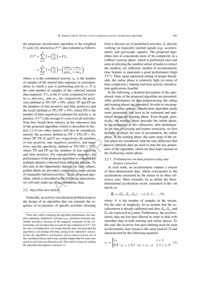
the proposed classification algorithm is the weightedf1 score [4], denoted as F1w and evaluated as follows:

F1w =A∑

a=1

2 ∗(na

N

)∗ F1a

=A∑

a=1

2 ∗(na

N

)∗

(preca ∗ reca

preca + reca

)where: a is the considered activity; na is the numberof samples of the inertial data sequence in correspon-dence to which a user is performing activity a; N isthe total number of samples of the collected inertialdata sequence; F1a is the f1 score computed for activ-ity a; and preca and reca are, respectively, the preci-sion (defined as TP/(TP + FP), where TP and FP arethe numbers of true positives and false positives) andthe recall (defined as TP/(TP + FN), where FN is thenumber of false negatives) evaluated for activity a. Inpractice, F1w is the average f1 score over all activities.Note that, beside these metrics, in the refinement stepof the proposed algorithm (which is described in Sec-tion 2.2.4) two other metrics will also be considered,namely: the accuracy, defined as (TP + TN)/(P + N),where TP, TN, P, and N are, respectively, the numbersof true positives, true negatives, positives, and nega-tives; and the specificity, defined as TN/(FP + TN),where TN and FP are the numbers of true negativesand false positives. For reproducibility purposes, theperformance of the proposed algorithm is evaluated formultiple datasets collected from different subjects. Tothis end, in the Opportunity dataset, for each subject,golden labels are provided, containing a single streamof (manually) labeled activities.2 In the proposed algo-rithm, which is described in the following subsections,we will only make use of accelerometric data.

2.2. Algorithm description

Generally, an activity classification problem leads tothe design of an algorithm that can estimate the se-quence of occurrences of specific activities choosing

2Note that, while evaluating the algorithm performance, the sam-ples containing “undefined” activities (e.g., transitions between clas-sifiable activities), because of the temporal continuity of the col-lected data, are not taken into account for the evaluation of F1w. Forthe sake of completeness, we remark that this does not mean that thealgorithm is not dealing with data coming from “unknown” classes.In fact, the algorithm is not forced to always choose at least one ofthe considered classes and it may actually happen that for some timeepoch no activities are detected at all. This will be clearer by readingthe algorithm description in Section 2.2.

from a discrete set of predefined activities A, directlyworking on (typically) inertial signals (e.g., accelero-metric and gyroscopic signals). The proposed algo-rithm tries to concentrate most of its complexity in a(offline) training phase, which is performed once andaims at selecting the smallest subset of nodes to extractthe smallest, yet sufficient, number of accelerometrictime features to guarantee a good performance (highF1w). Then, upon optimized setting of proper thresh-olds, the online phase is relatively light (in terms oftime complexity), making real-time activity classifica-tion applications feasible.

In the following, a detailed description of the oper-ational steps of the proposed algorithm are presented.After preliminaries on data preprocessing, the onlineand training phases are presented. In order to run prop-erly, the online activity classification algorithm needssome parameters that have to be estimated and opti-mized during the training phase. Even though, prac-tically, the training phase precedes the online phase,in the remainder of this subsection, after preliminar-ies on data processing and feature extraction, we firstdescribe in detail, for ease of presentation, the onlinephase. In the training phase, the same steps of the on-line phase are considered, with the only difference thatknown (labeled) data are used to tune the key param-eters of the algorithm, which are then kept constant inthe (following) online phase.

2.2.1. Preliminaries on data preprocessing andfeature extraction

At each node, an accelerometer outputs a streamof three-dimensional data, which corresponds to theaccelerations measured by the sensor in its three ref-erence axes. More formally, let us define the three-dimensional acceleration vector, measured at the i-thepoch, as

α̃i = (̃αxi , α̃yi , α̃zi) i ∈ {1, 2, . . . , N}where N is the number of samples in the stream.For the sake of simplicity, let us assume that the ac-celerometer is already calibrated and, thus, α̃xi, α̃yi, andα̃zi are expressed in g units. Furthermore, the accelero-metric data are low-pass filtered in order to deal withsmoother data in both training and online phases. Tothis end, the recursive low-pass filtering used for eachaccelerometric data stream is the same used in [7] andcharacterized by the following equation:

yi ={

x1 i = 1

0.8 · yi−1 + 0.1 · (xi + xi−1) 2 � i � N(1)

AUTHOR COPY

684 M. Giuberti and G. Ferrari / A low-complexity activity classification algorithm

where xi is the i-th sample of the data stream (x ∈{̃αx, α̃y, α̃z}), yi is the i-th sample of the filtered datastream (y ∈ {αx, αy, αz}). The cut-off frequency fco of

the low-pass filter defined in (1) is fco ≈ fsamp30 = 1 Hz.

Therefore, we denote the filtered signal as

αi = (αxi, αyi, αzi) i ∈ {1, 2, . . . , N}and the norm of αi as

αi = |αi | =√

α2xi + α2

yi + α2zi i ∈ {1, 2, . . . , N}.

Starting from the filtered signal, at the i-th epoch,two types of simple features are of interest and canbe extracted. The first one, denoted as p-feature(where “p” stands for “parallel”) and indicated withacc(p)

i , is a properly chosen component of the nor-

malized3 (to unity) acceleration vector, i.e., acc(p)

i ∈{αxi/|αi |, αyi/|αi |, αzi/|αi |}. In particular, the chosencomponent is the one parallel to the “main” axis ofthe related body segment. For instance, consideringFig. 1: for node 1, acc(p)

i is the acceleration valuemeasured along the femur direction; for node 7, theone measured along the tibia. Observe that, due to thenormalization, acc(p)

i can only assume real values in[−1,+1].

The second considered feature, denoted as dev-feature and indicated with σi(s), is the standard devi-ation of the norm of the acceleration computed on asliding window (with fixed length L = 2 · s + 1 andcentered at the i-th sample4) that runs over all the ac-celeration samples. Neglecting border effects (the ex-tension is straightforward, as shown in [8]), σi(s) canbe expressed as follows:

σi(s) =√∑i+s

k=i−s[αk − μk(s)]2

L − 1(2)

where

μk(s) �∑i+s

k=i−s αk

L − 1. (3)

3Note that, by normalizing the acceleration vector (for the p-feature), we are implicitly assuming that no linear acceleration ispresent (i.e., the device is still) and only the gravity acceleration con-tribution (i.e., 1 g) is measured by the accelerometer. Note that, al-though this assumption is not always true, in the majority of humanmovements it is true that the magnitude of the linear acceleration israther lower than that of the gravity component.

4More details about the definition of the window, especially at theborders of the acceleration signal, are given in [8].

It can be observed that σi(s) is always larger than orequal to 0 – typically, it is not considerably larger than1 (due to the expression of the accelerometric data in gunits). While evaluating the classification performanceof the proposed algorithm, s is set to 7 samples and,therefore, the dev-features are computed on a windowof length L = 15 samples (i.e., 0.5 s).

2.2.2. The general ideaConsidering a single activity a ∈ A, the output of

an activity classification algorithm is given by a binarysequence w(a) = (w1(a), w2(a), . . . , wN(a)) wherewi(a) = 0 if a is not detected at epoch i (the indexi runs over the samples of the collected acceleromet-ric data sequence) or wi(a) = 1 if a is detected. Inparticular, w(a) contains “activity windows” (disjointgroups of consecutive “1”s), within which the activitya has been detected. The length of each activity win-dow is recursively determined – using three parame-ters �1, �2, and �3, optimized independently for eachactivity. This process will be described later.

For each considered activity, the proposed activityclassification algorithm aims at automatically selectingthe best nodes in the BSN and the corresponding mostsignificant feature types, that can best discriminate theoccurrence of the considered activity (e.g., the thighnode is intuitively one of the best nodes to estimate a“sit” activity, whereas the feet nodes give relevant in-formation about the “walk” activity). More formally,let us define as F = {f1, f2, . . . , fF } (with cardinality|F | = F ) a set of features where the generic featuref ∈ F corresponds to a feature “type” (p-feature ordev-feature) associated with a specific node. As an ex-ample, referring to Fig. 1, f = 1p is the p-feature ex-tracted from the thigh node (i.e., node 1) and f = 7dis the dev-feature extracted from the tibia node (i.e.,node 7). In the following, when referring to the valueof a feature, we will implicitly refer to the value of the“embedded” feature type. Furthermore, given a spe-cific activity a, C∗

a ⊂ F represents the subset of themost significant features used to classify activity a.5

The proposed algorithm identifies activities by prop-erly thresholding the selected features. In particular,referring to a given feature f , an activity a is consid-

5Note that, throughout this paper, the term “optimal” and the su-perscript “*” are equivalently used with reference to the tunable pa-rameters considered in the proposed algorithm. Furthermore, if notstated otherwise, the optimality is always intended in terms of clas-sification performance through the f1 score (when activities are in-dependently considered) and the weighted f1 score (when activitiesare combined together).

AUTHOR COPY

M. Giuberti and G. Ferrari / A low-complexity activity classification algorithm 685

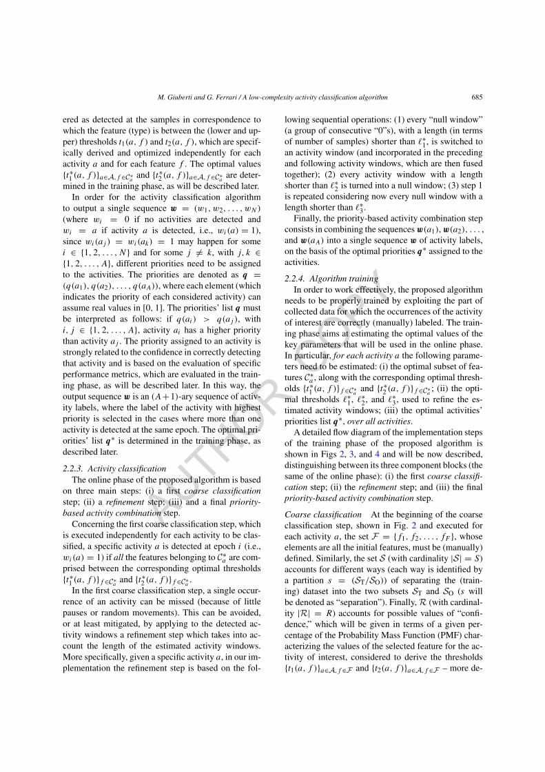
ered as detected at the samples in correspondence towhich the feature (type) is between the (lower and up-per) thresholds t1(a, f ) and t2(a, f ), which are specif-ically derived and optimized independently for eachactivity a and for each feature f . The optimal values{t∗1 (a, f )}a∈A,f ∈C∗

aand {t∗2 (a, f )}a∈A,f ∈C∗

aare deter-

mined in the training phase, as will be described later.In order for the activity classification algorithm

to output a single sequence w = (w1, w2, . . . , wN)

(where wi = 0 if no activities are detected andwi = a if activity a is detected, i.e., wi(a) = 1),since wi(aj ) = wi(ak) = 1 may happen for somei ∈ {1, 2, . . . , N} and for some j �= k, with j, k ∈{1, 2, . . . , A}, different priorities need to be assignedto the activities. The priorities are denoted as q =(q(a1), q(a2), . . . , q(aA)), where each element (whichindicates the priority of each considered activity) canassume real values in [0, 1]. The priorities’ list q mustbe interpreted as follows: if q(ai) > q(aj ), withi, j ∈ {1, 2, . . . , A}, activity ai has a higher prioritythan activity aj . The priority assigned to an activity isstrongly related to the confidence in correctly detectingthat activity and is based on the evaluation of specificperformance metrics, which are evaluated in the train-ing phase, as will be described later. In this way, theoutput sequence w is an (A+1)-ary sequence of activ-ity labels, where the label of the activity with highestpriority is selected in the cases where more than oneactivity is detected at the same epoch. The optimal pri-orities’ list q∗ is determined in the training phase, asdescribed later.

2.2.3. Activity classificationThe online phase of the proposed algorithm is based

on three main steps: (i) a first coarse classificationstep; (ii) a refinement step; (iii) and a final priority-based activity combination step.

Concerning the first coarse classification step, whichis executed independently for each activity to be clas-sified, a specific activity a is detected at epoch i (i.e.,wi(a) = 1) if all the features belonging to C∗

a are com-prised between the corresponding optimal thresholds{t∗1 (a, f )}f ∈C∗

aand {t∗2 (a, f )}f ∈C∗

a.

In the first coarse classification step, a single occur-rence of an activity can be missed (because of littlepauses or random movements). This can be avoided,or at least mitigated, by applying to the detected ac-tivity windows a refinement step which takes into ac-count the length of the estimated activity windows.More specifically, given a specific activity a, in our im-plementation the refinement step is based on the fol-

lowing sequential operations: (1) every “null window”(a group of consecutive “0”s), with a length (in termsof number of samples) shorter than �∗

1, is switched toan activity window (and incorporated in the precedingand following activity windows, which are then fusedtogether); (2) every activity window with a lengthshorter than �∗

2 is turned into a null window; (3) step 1is repeated considering now every null window with alength shorter than �∗

3.Finally, the priority-based activity combination step

consists in combining the sequences w(a1), w(a2), . . . ,and w(aA) into a single sequence w of activity labels,on the basis of the optimal priorities q∗ assigned to theactivities.

2.2.4. Algorithm trainingIn order to work effectively, the proposed algorithm

needs to be properly trained by exploiting the part ofcollected data for which the occurrences of the activityof interest are correctly (manually) labeled. The train-ing phase aims at estimating the optimal values of thekey parameters that will be used in the online phase.In particular, for each activity a the following parame-ters need to be estimated: (i) the optimal subset of fea-tures C∗

a , along with the corresponding optimal thresh-olds {t∗1 (a, f )}f ∈C∗

aand {t∗2 (a, f )}f ∈C∗

a; (ii) the opti-

mal thresholds �∗1, �∗

2, and �∗3, used to refine the es-

timated activity windows; (iii) the optimal activities’priorities list q∗, over all activities.

A detailed flow diagram of the implementation stepsof the training phase of the proposed algorithm isshown in Figs 2, 3, and 4 and will be now described,distinguishing between its three component blocks (thesame of the online phase): (i) the first coarse classifi-cation step; (ii) the refinement step; and (iii) the finalpriority-based activity combination step.

Coarse classification At the beginning of the coarseclassification step, shown in Fig. 2 and executed foreach activity a, the set F = {f1, f2, . . . , fF }, whoseelements are all the initial features, must be (manually)defined. Similarly, the set S (with cardinality |S| = S)accounts for different ways (each way is identified bya partition s = (ST/SO)) of separating the (train-ing) dataset into the two subsets ST and SO (s willbe denoted as “separation”). Finally, R (with cardinal-ity |R| = R) accounts for possible values of “confi-dence,” which will be given in terms of a given per-centage of the Probability Mass Function (PMF) char-acterizing the values of the selected feature for the ac-tivity of interest, considered to derive the thresholds{t1(a, f )}a∈A,f ∈F and {t2(a, f )}a∈A,f ∈F – more de-

AUTHOR COPY

686 M. Giuberti and G. Ferrari / A low-complexity activity classification algorithm

Fig. 2. Detailed flow diagram of the implementation steps of the proposed algorithm’s training phase: the first coarse classification step.

tails about confidence are provided below with an ex-ample. Note that the separation into the two subsets ST

and SO is done in order to cross-validate the statistical

performance of the algorithm, i.e., to assess how thealgorithm’s performance will generalize with an inde-pendent dataset. In the machine learning field, this is a

AUTHOR COPY

M. Giuberti and G. Ferrari / A low-complexity activity classification algorithm 687

Fig. 3. Detailed flow diagram of the implementation steps of the proposed algorithm’s training phase: the refinement step.

common practice used to derive unbiased performanceof an algorithm, especially when only training data areavailable [5].

The goal of the first part of the coarse classifica-tion step is to estimate and store the activity win-dows {w(a, f, r, s)}a∈A,f ∈F ,r∈R,s∈S . As already ex-

AUTHOR COPY

688 M. Giuberti and G. Ferrari / A low-complexity activity classification algorithm

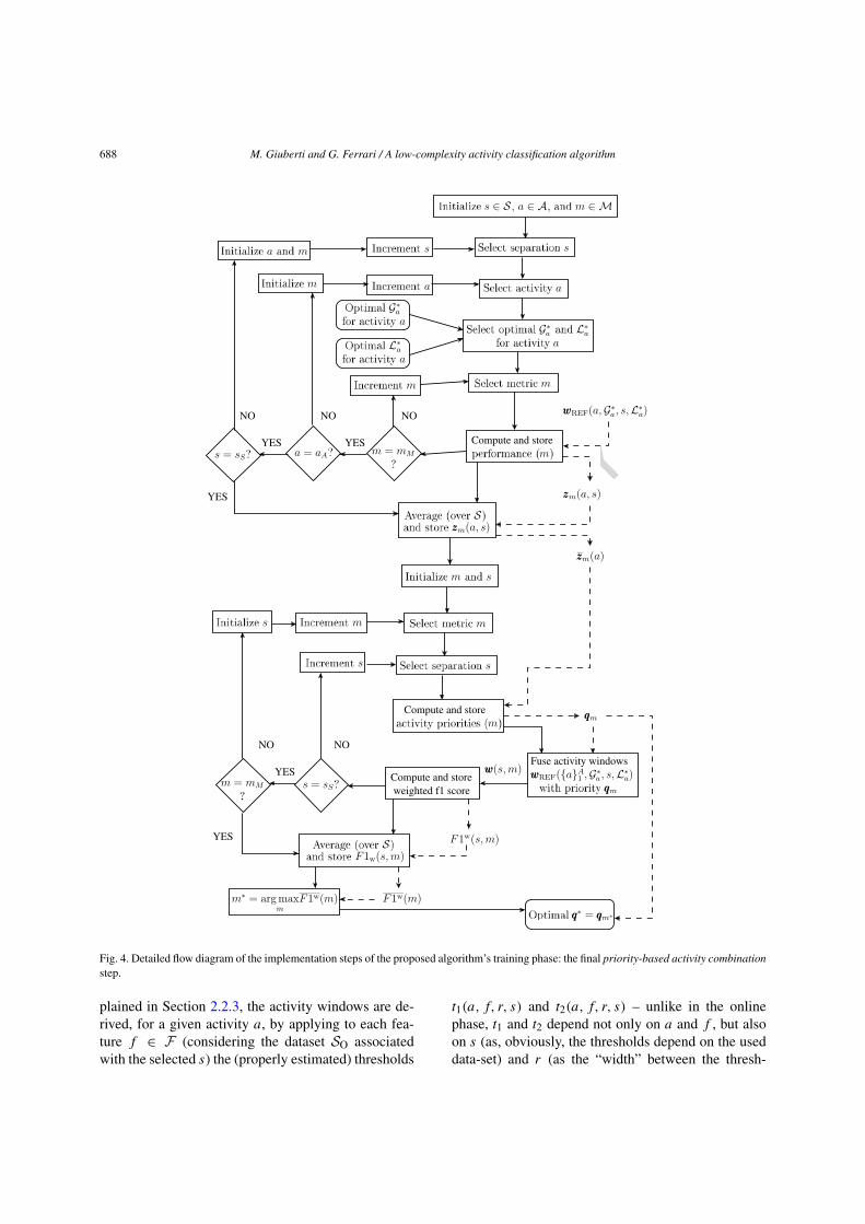
Fig. 4. Detailed flow diagram of the implementation steps of the proposed algorithm’s training phase: the final priority-based activity combinationstep.

plained in Section 2.2.3, the activity windows are de-rived, for a given activity a, by applying to each fea-ture f ∈ F (considering the dataset SO associatedwith the selected s) the (properly estimated) thresholds

t1(a, f, r, s) and t2(a, f, r, s) – unlike in the onlinephase, t1 and t2 depend not only on a and f , but alsoon s (as, obviously, the thresholds depend on the useddata-set) and r (as the “width” between the thresh-

AUTHOR COPY

M. Giuberti and G. Ferrari / A low-complexity activity classification algorithm 689

olds depend on the desired confidence – the larger, thehigher the required confidence).

In order to clarify the process which leads to theidentification of the thresholds for activity classifica-tion, we consider an example relative to the acceler-ation signals produced at the thigh node (i.e., node 1in Fig. 1) and used to detect the “sit” activity. An il-lustrative description of the thresholds estimation stepis shown in Fig. 5: the p-feature (i.e., f = 1p) andthe dev-feature (i.e., f = 1d), shown in Fig. 5(b),are first extracted from the acceleration signals (shownin Fig. 5(a), in the x, y, and z axes) and evaluateddiscretely in the “sit” intervals (assuming that a =sit and for a given s ∈ S) in order to obtain theirPMFs in such intervals (the PMFs of the p-featureand the dev-feature are shown in Figs 5(c) and 5(d),respectively). Given a, f , s, for each value of r ∈R, the thresholds t1(a, f, r, s) and t2(a, f, r, s) arethen chosen as the extremes of the shortest interval(t1, t2) which comprises at least r% of the probabilitymass.

The second part of the coarse classification step, stillperformed independently for each a ∈ A, is based onthe fusion of different combinations of the previouslystored activity windows {w(a, f, r, s)}f ∈F ,r∈R,s∈S .The goal is to find, for each activity, the optimal com-bination G∗

a (among the G possible combinations),where the generic combination Ga is associated witha possible subset of features Ca ⊂ F and two val-ues of r , i.e., rp and rdev, from which the thresholdst1(a, f, r, s) and t2(a, f, r, s) can be estimated whenthe considered f is, respectively, a p-feature or a dev-feature. An example, a possible instance of Ga couldbe (Ca = {1d, 1p, 4p}, rp = 93%, rdev = 97%).

Given a combination Ga and a separation s ∈S , the set Wa(Ga, s) is defined as the subset of{w(a, f, r, s)}f ∈F ,r∈R with (f, r) ∈ Ga . The se-quences of activity windows in Wa(Ga, s) are thenfused together (and stored for future use) into a sin-gle sequence of activity windows w(a,Ga, s), ob-tained from the “logical AND” of all the consid-ered sequences of activity window. The f1 score ofw(a,Ga, s), denoted as F1a(Ga, s), is then computedand stored. By averaging {F1a(Ga, s)}s∈S over all pos-sible separations in S and denoting this average asF1a(Ga) = ∑

s∈S F1a(Ga, s)/S, the optimal G∗a is

selected as follows:

G∗a = arg max

Ga

F1a(Ga). (4)

Fig. 5. Description of the thresholds estimation step, which appearsin Fig. 2, for an illustrative acceleration signal produced at the thighnode: (a) acceleration signal (the x, y, and z components are high-lighted); (b) p-feature (straight line) and dev-feature (dashed line)extracted from the previous acceleration signal; PMFs of (c) p-fea-ture and (d) dev-feature evaluated in the “sit” intervals.

AUTHOR COPY

690 M. Giuberti and G. Ferrari / A low-complexity activity classification algorithm

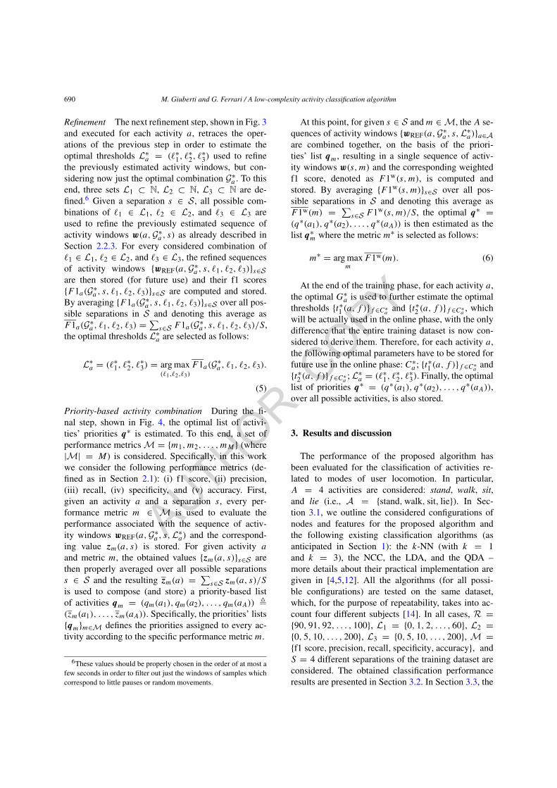
Refinement The next refinement step, shown in Fig. 3and executed for each activity a, retraces the oper-ations of the previous step in order to estimate theoptimal thresholds L∗

a = (�∗1, �

∗2, �

∗3) used to refine

the previously estimated activity windows, but con-sidering now just the optimal combination G∗

a . To thisend, three sets L1 ⊂ N, L2 ⊂ N, L3 ⊂ N are de-fined.6 Given a separation s ∈ S , all possible com-binations of �1 ∈ L1, �2 ∈ L2, and �3 ∈ L3 areused to refine the previously estimated sequence ofactivity windows w(a,G∗

a , s) as already described inSection 2.2.3. For every considered combination of�1 ∈ L1, �2 ∈ L2, and �3 ∈ L3, the refined sequencesof activity windows {wREF(a,G∗

a , s, �1, �2, �3)}s∈Sare then stored (for future use) and their f1 scores{F1a(G∗

a , s, �1, �2, �3)}s∈S are computed and stored.By averaging {F1a(G∗

a , s, �1, �2, �3)}s∈S over all pos-sible separations in S and denoting this average asF1a(G∗

a , �1, �2, �3) = ∑s∈S F1a(G∗

a , s, �1, �2, �3)/S,the optimal thresholds L∗

a are selected as follows:

L∗a = (�∗

1, �∗2, �

∗3) = arg max

(�1,�2,�3)

F1a(G∗a , �1, �2, �3).

(5)

Priority-based activity combination During the fi-nal step, shown in Fig. 4, the optimal list of activi-ties’ priorities q∗ is estimated. To this end, a set ofperformance metrics M = {m1,m2, . . . , mM } (where|M| = M) is considered. Specifically, in this workwe consider the following performance metrics (de-fined as in Section 2.1): (i) f1 score, (ii) precision,(iii) recall, (iv) specificity, and (v) accuracy. First,given an activity a and a separation s, every per-formance metric m ∈ M is used to evaluate theperformance associated with the sequence of activ-ity windows wREF(a,G∗

a , s,L∗a) and the correspond-

ing value zm(a, s) is stored. For given activity a

and metric m, the obtained values {zm(a, s)}s∈S arethen properly averaged over all possible separationss ∈ S and the resulting zm(a) = ∑

s∈S zm(a, s)/S

is used to compose (and store) a priority-based listof activities qm = (qm(a1), qm(a2), . . . , qm(aA)) �(zm(a1), . . . , zm(aA)). Specifically, the priorities’ lists{qm}m∈M defines the priorities assigned to every ac-tivity according to the specific performance metric m.

6These values should be properly chosen in the order of at most afew seconds in order to filter out just the windows of samples whichcorrespond to little pauses or random movements.

At this point, for given s ∈ S and m ∈ M, the A se-quences of activity windows {wREF(a,G∗

a , s,L∗a)}a∈A

are combined together, on the basis of the priori-ties’ list qm, resulting in a single sequence of activ-ity windows w(s,m) and the corresponding weightedf1 score, denoted as F1w(s,m), is computed andstored. By averaging {F1w(s,m)}s∈S over all pos-sible separations in S and denoting this average asF1w(m) = ∑

s∈S F1w(s,m)/S, the optimal q∗ =(q∗(a1), q

∗(a2), . . . , q∗(aA)) is then estimated as the

list q∗m where the metric m∗ is selected as follows:

m∗ = arg maxm

F1w(m). (6)

At the end of the training phase, for each activity a,the optimal G∗

a is used to further estimate the optimalthresholds {t∗1 (a, f )}f ∈C∗

aand {t∗2 (a, f )}f ∈C∗

a, which

will be actually used in the online phase, with the onlydifference that the entire training dataset is now con-sidered to derive them. Therefore, for each activity a,the following optimal parameters have to be stored forfuture use in the online phase: C∗

a ; {t∗1 (a, f )}f ∈C∗a

and{t∗2 (a, f )}f ∈C∗

a; L∗

a = (�∗1, �

∗2, �

∗3). Finally, the optimal

list of priorities q∗ = (q∗(a1), q∗(a2), . . . , q

∗(aA)),over all possible activities, is also stored.

3. Results and discussion

The performance of the proposed algorithm hasbeen evaluated for the classification of activities re-lated to modes of user locomotion. In particular,A = 4 activities are considered: stand, walk, sit,and lie (i.e., A = {stand, walk, sit, lie}). In Sec-tion 3.1, we outline the considered configurations ofnodes and features for the proposed algorithm andthe following existing classification algorithms (asanticipated in Section 1): the k-NN (with k = 1and k = 3), the NCC, the LDA, and the QDA –more details about their practical implementation aregiven in [4,5,12]. All the algorithms (for all possi-ble configurations) are tested on the same dataset,which, for the purpose of repeatability, takes into ac-count four different subjects [14]. In all cases, R ={90, 91, 92, . . . , 100}, L1 = {0, 1, 2, . . . , 60}, L2 ={0, 5, 10, . . . , 200}, L3 = {0, 5, 10, . . . , 200}, M ={f1 score, precision, recall, specificity, accuracy}, andS = 4 different separations of the training dataset areconsidered. The obtained classification performanceresults are presented in Section 3.2. In Section 3.3, the

AUTHOR COPY

M. Giuberti and G. Ferrari / A low-complexity activity classification algorithm 691

time complexity of all considered algorithms is sum-marized. Finally, in Section 3.4 the robustness of theproposed algorithm against rotational noise is investi-gated, as this is particularly meaningful for BSN-basedactivity classification applications.

3.1. Configurations of nodes and features

Overall, we consider 38 different configurations ofnodes (and feature types): configurations 1–31 (with atmost 7 nodes) apply to the proposed algorithms andthe four considered existing classification algorithms(k-NN, NCC, LDA, and QDA) and rely on the use ofaccelerometric data; configurations 32–38 (with morethan 7 nodes) apply only to the four considered ex-isting classification algorithms and rely on the use ofother (besides accelerometers) inertial sensors (e.g.,magnetometers). Each configuration involves a spe-cific nodes’ configuration, explicitly shown in the x

axis of Fig. 6 (which will be described in the next sub-section) with reference to the node number in Fig. 1.

Note that, given a set of activities that need to beclassified, the number and placement of the devicescould be preliminary devised and used by determin-ing which devices may provide the most different sig-nal patterns in correspondence to different activities.However, in this work we take advantage of the factthat an exhaustive dataset was provided in the Oppor-tunity Challenge [4,14,18], since the BSN used to ac-quire the given dataset was composed by a large num-ber of sensor devices placed all over the users’ body.The automatic selection of the best devices and fea-tures is then left to the “artificial intelligence” of the al-gorithm (specifically, during the training phase). In thisway, some sensor devices, which could have appearedto be intuitively useless at classifying some activities,may be instead selected as good candidates. Further-more, once the best set of devices is determined, theproposed approach also allows to automatically deter-mine the best subset of devices and features for eachactivity that has to be classified and such subset maylikely change from activity to activity.

The choice of the nodes’ feature types for each clas-sification algorithm can be summarized as follows.

– Configurations 1–31; proposed algorithm. On-ly p-features and dev-features are considered.Specifically: for nodes 7, 1, 2, and 6 (namely,the nodes of the main vertical segment of the hu-man body) both types of features are extracted;for nodes 13, 19, and 21 (feet nodes and a second

Fig. 6. Average (over 4 subjects) classification performance (i.e.,weighted f1 score) as a function of the considered configurationsof nodes. The performance of the proposed algorithm is comparedwith that of some existing algorithms, averaging the performance ofthe four considered subjects. For every configuration, the consideredsubsets of BSN nodes (numbered as in Fig. 1) are highlighted. Thefeatures per configuration and per algorithm are properly selected assummarized in Section 3.1.

node for the back) only the d-feature is extracted.In particular, at most F = 11 features are consid-ered (for instance, the set of features of Config-uration 1 is F = {1p, 2p, 6p, 7p, 1d, 2d, 6d, 7d,

13d, 19d, 21d}).– Configurations 1–31; k-NN, NCC, LDA, and

QDA algorithms. For all the nodes, the meanof every acceleration component within a slidingwindow is considered, leading to 3 features ex-tracted at each node. Therefore, at most F = 21features are considered.

– Configurations 32–38; k-NN, NCC, LDA, andQDA algorithms. For all the nodes, the meanof every acceleration component within a slid-ing window is still considered (as in the previouscase). In addition, for configurations from 34 to38, the mean within a sliding window is also com-puted for the 3 components of the gyroscope andmagnetometer signals, or some combinations ofthem, as summarized below:

∗ for configuration 34: every node equipped withgyroscope and magnetometer (i.e., nodes from13 to 21) produces 6 additional features (3from gyroscope and 3 from magnetometer);

∗ for configuration 35: 6 additional features (3from gyroscope and 3 from magnetometer) areextracted at node 13;

AUTHOR COPY

692 M. Giuberti and G. Ferrari / A low-complexity activity classification algorithm

Fig. 7. Average (over 4 subjects) classification performance (i.e., weighted f1 score) as a function of the considered (a) number of nodes and(b) number of features. For each considered algorithm, the configurations which use the same number of (a) nodes or (b) features have beenaveraged together.

∗ for configuration 36: 3 additional gyroscopicfeatures are extracted at node 13;

∗ for configurations 37 and 38: 3 additional mag-netometric features are extracted at node 13.

3.2. Classification performance

The performance of the proposed algorithm hasbeen evaluated for 31 different configurations of nodesin order to determine the optimal subset of BSN nodes(and, thus, of features) useful for the activity classifica-tion. In particular, in Fig. 6, the performance of our al-gorithm (in terms of F1w) is shown as a function of theconfigurations of nodes, averaging over the consideredfour subjects. A comparison with the performance ob-tained with the other considered algorithms, run withthe same configurations of nodes, is also shown. Notethat the performance of these algorithms is also eval-uated for more complex configurations of nodes (fora total of 38 configurations), which consider the useof a larger number of nodes and features. It is easy toobserve that, in most of the considered configurationsof nodes, our algorithm outperforms the other ones.It can also be seen that some of the reference algo-rithms (in particular, k-NN and QDA) have similar per-formance to ours, but only when considering, in theircases, more complex configurations with larger num-bers of nodes and features. Note also that the central“hole” in Fig. 1 is associated with those configurationsof nodes (namely, 15, 16, 17, 18, and 21 in Fig. 6)which do not use node 1 (the thigh node) in Fig. 1,i.e., a key node in discriminating between sit and standactivities. A similar observation can be made for con-

figuration 31 (as denoted in Fig. 6), which hardly dis-criminates between stand and walk due to the absenceof both feet nodes (namely, nodes 19 and 21 in Fig. 1).

In order to better investigate the impact of the num-ber of nodes on the performance of the considered al-gorithms, in Fig. 7(a) the performance of the consid-ered algorithms is properly averaged over all configu-rations with the same number of nodes. It can be ob-served that, for a given number of nodes in the BSN,our algorithm, making use of configurations with atmost 7 nodes, outperforms the others. Moreover, withonly 7 nodes, our algorithm outperforms all existingalgorithms, including the k-NN and QDA, run with amuch larger number of nodes (e.g., 21).

Another aspect to take into account is the numberof features used in the algorithms. Unlike the existingalgorithms, where each node generates at least threefeatures,7 our algorithm is such that a maximum oftwo features (i.e., the p-feature and the dev-feature)can be extracted at each node. In Fig. 7(b), it is thenshown how the algorithms’ performance changes withrespect to the considered overall number of features(over all nodes). It can be concluded that our algorithmprovides the same, or even better, performance, withrespect to the other algorithms, using a significantlysmaller number of features. The number of used fea-tures has a significant impact on the time complexity

7The typical features computed at each node are the mean of everyacceleration component within a sliding window. In addition, othersix features are considered for nodes provided with gyroscopes andmagnetometers. A standard deviation-related feature has been alsoused giving however poor performance.

AUTHOR COPY

M. Giuberti and G. Ferrari / A low-complexity activity classification algorithm 693

of a classification algorithm, as it will be explainedin Section 3.3, allowing a better real-time applicabil-ity of our algorithm with respect to the others. As pre-viously observed, k-NN and QDA are the only algo-rithms which can achieve, for a very large number offeatures (over 110), a performance similar to that ofour algorithm (using only 11 features).

For the sake of completeness, we want to highlightthat, if the previously cited configurations 15, 16, 17,18, 21 in Fig. 6 (which do not use node 1 in Fig. 1) arenot taken into account for the evaluation of the curvesin Fig. 7, the performance of our algorithm improvessignificantly more (in relative terms) than those of theother algorithms.

Finally, on the basis of the previous results, config-uration 22 (as denoted in Fig. 6) can be identified asthe best configuration of nodes for our algorithm. Inparticular, it needs 5 nodes (namely, nodes {1, 2, 13,19, 21} in Fig. 1) and generates F = 7 features (5dev-features, one per node, and 2 p-features, associ-ated with nodes 1 and 2 in Fig. 1). Using this config-uration, our algorithm obtains a value of F1w around85%. The second best algorithm, i.e., the k-NN (withk = 3), reaches a value of F1w around 77% using15 features (more than twice the number in our al-gorithm) and more sensors (indeed, gyroscopes andmagnetometers are available in nodes {13, 19, 21} inFig. 1). Furthermore, the best among the other algo-rithms (again, the k-NN with k = 3) obtains its highestF1w score (namely, F1w = 84%) using a significantlymore complex configuration (namely, configuration 34in Fig. 6), which comprises a total of 21 nodes andF = 113 features.

3.3. Time complexity

The time complexity of the proposed algorithm hasbeen evaluated and compared with those of the clas-sification algorithms previously considered for per-formance comparison.8 In particular, it is possible toprove that the time complexity of the online phase ofour algorithm is a linear function of the number of fea-tures F and the number of activities A. In Table 1,the time complexity of our algorithm is reported alongwith those of the other considered algorithms [5,12].

8Recall that, we here consider the time complexity of the onlinephase due to its impact on real-time applicability of the algorithmand due to the fact that the training phase should be performed justonce (offline), provided that the BSN configuration does not changeover time.

Table 1

Time complexity of the online phase for the considered algorithms

Algorithm Time Complexity

proposed, NCC, LDA, and QDA O(F · A)

k-NN O(F · D)

It can be observed that the time complexity of all al-gorithms is a linear function of the number of fea-tures F . In addition, our algorithm, the NCC, LDA,and QDA algorithms have a complexity linearly de-pendent on the number of activities A, but independentof the training dataset size D, whereas the time com-plexity of the k-NN algorithm depends linearly on D

and is independent of A. Two considerations can nowbe made about A, D, and F :

– the number of activities is typically quite largerthan the size of the training dataset (i.e., A � D);

– the classification performance of the proposed al-gorithm, when considering a few features (i.e.,for small values of F ), is far better than those ofthe NCC, the LDA, and the QDA algorithms (andalso slightly better than that of the k-NN algo-rithm).

For these reasons, it can be concluded that our al-gorithm (i) guarantees the best compromise betweenclassification performance and time complexity and(ii) outperforms, for a given number of features, theother algorithms.

3.4. Robustness to noise of the proposed algorithm

A typical problem of a real BSN scenario consistsof unwanted rotations in the displacement of the BSNnodes, that can differ between the training and theonline phases. It is then of interest to investigate therobustness of BSN-based activity classification algo-rithm to rotational noise. To this end, artificial ro-tational noise has been added to the accelerometricdata, simulating possible rotations of a device aroundits three reference axes. We remark that modelingrotations around the accelerometer axes, rather thanaround the body axes, is just an assumption, which ismade to avoid taking devices position shifts also intoaccount. It is, however, a reasonable assumption, sincethe position shifts would be rather limited.

Two considerations can be preliminary made: thedev-feature is actually insensitive to rotational noise,due to its definition; the p-feature is invariant to rota-tional noise around the axis about which the featureis measured (i.e., the one parallel to the related body

AUTHOR COPY

694 M. Giuberti and G. Ferrari / A low-complexity activity classification algorithm

Fig. 8. Average (over 4 subjects) classification performance (i.e., weighted f1 score) of the proposed algorithm in the presence of simulatedrotational noise: (a) the weighted f1 score as a function of the intensity of the simulated rotational noise; (b) the admissible range of rotationsas a function of the weighted f1 score. The previously estimated optimal configuration of nodes (i.e., configuration 22, as denoted in Fig. 6) isconsidered. Indicative thresholds (dashed lines), corresponding to an admissible minimum performance of F1w = 70%, are also shown in twosubfigures.

segment, which we assume to be the y axis for everydevice). For such reasons, the rotational noise is thenbeing only added to p-features and the device rotationshave been simulated only around its other two axes,namely (due to the previous assumption) the x and z

axes. More specifically, from now on, we assume thatthe x axis is directed from the front to the back of theuser, whereas the z axis is directed from his/her rightside to his/her left side. For ease of simplicity, we onlysimulate rotations around one axis at a time.

In Fig. 8(a), the average performance of our al-gorithm (averaged over the 4 considered subjects) isshown as a function of the intensity of the simulatedrotational noise (in terms of degrees of rotation with re-spect to the initial orientation), for the previously esti-mated (at the end of Section 3.2) optimal configurationof nodes (i.e., configuration 22, as denoted in Fig. 6).In Fig. 8(b), for the same configuration 22 (as denotedin Fig. 6) and averaging over the same 4 subjects, thecurves show the range of rotations that can be appliedto the nodes in order to keep a user-defined admissibleminimum performance (in terms of weighted f1 score).The results in Fig. 8 show that our algorithm, possi-bly due to the nature of the activities that we want toclassify, suffers less from rotations around the z axisthan those around the x axis. As an example, if oneaccepts as a minimum acceptable performance a F1w

equal to 70%, a system using the proposed algorithmcan tolerate rotations in the range of [−10◦, 10◦].

We also remark that, due to the realistic data collec-tion (often operated in different times with respect to

the training acquisition), the testing data (used in theonline phase) implicitly presents real rotational noise.Therefore, the results previously presented implicitlyassume that the proposed algorithm has to combatsome rotational noise.

4. Conclusion

In this work, a simple, yet effective, activity classi-fication algorithm has been presented. Its performancehas been evaluated and compared with that of exist-ing algorithms. The data used to test the algorithmsare publicly available and, thus, represent a valid andunbiased benchmark for the evaluation of the perfor-mance of different algorithms. The proposed algorithmis based on simple comparisons of properly selectedfeatures with thresholds that are automatically opti-mized during a preliminary training phase performedonce (offline). In order to simplify the operations ofthe online phase of the algorithm, the training phase isalso used to automatically select the optimal subset ofnodes and features to be used.

The time complexity of the proposed algorithm hasalso been evaluated. Our results show that its complex-ity is on the order of that of existing algorithms, butits performance is better. On the other hand, some ofthe existing algorithms show a performance similar tothat of ours at the cost of higher complexity. In partic-ular, our algorithm significantly outperforms the oth-ers when using a small numbers of nodes and features.

AUTHOR COPY

M. Giuberti and G. Ferrari / A low-complexity activity classification algorithm 695

Taking also into account its robustness against rota-tional noise, it can be concluded that the proposed al-gorithm can be used effectively for real-time activityclassification, especially when some constraints on thenumber of BSN nodes are introduced.

References

[1] R. Aylward and J. Paradiso, A compact, high-speed, wearablesensor network for biomotion capture and interactive media,in: Proc. of the 6th International Conference on InformationProcessing in Sensor Networks (IPSN), Cambridge, MA, USA,April 2007, pp. 380–389. doi:10.1145/1236360.1236408.

[2] L. Bao and S. Intille, Activity recognition from user annotatedacceleration data, in: Pervasive Computing, April 2004, pp. 1–17. doi:10.1007/978-3-540-24646-6_1.

[3] R. Chavarriaga, H. Bayati and J.d.R. Millán, Unsupervisedadaptation for acceleration-based activity recognition: Robust-ness to sensor displacement and rotation, Personal and Ubiq-uitous Computing 17(3) (March 2013), 479–490. doi:10.1007/s00779-011-0493-y.

[4] R. Chavarriaga, H. Sagha, A. Calatroni, S.T. Digumarti,G. Troster, J.d.R. Millan and D. Roggen, The opportunity chal-lenge: A benchmark database for on-body sensor-based activ-ity recognition, Pattern Recognition Letters 34(15) (November2013), 2033–2042. doi:10.1016/j.patrec.2012.12.014.

[5] R.O. Duda, P.E. Hart and D.G. Stork, Pattern Classificationand Scene Analysis, 2nd edn, Wiley-Interscience, New York,NY, USA, 2000.

[6] A. Fleury, M. Vacher and N. Noury, SVM-based multimodalclassification of activities of daily living in health smarthomes: Sensors, algorithms, and first experimental results,IEEE Trans. on Information Technology in Biomedicine 14(2)(March 2010), 274–283. doi:10.1109/TITB.2009.2037317.

[7] M. Giuberti and G. Ferrari, Simple and robust BSN-based ac-tivity classification: Winning the first BSN contest, in: Proc.4th International Symposium on Applied Sciences in Biomed-ical and Communication Technologies (ISABEL), Barcelona,Spain, October 2011.

[8] M. Giuberti and G. Ferrari, BSN-based activity classification:A low complexity windowing-&-classification approach, Ad-vances in Science and Technology 85 (2013), 53–58. doi:10.4028/www.scientific.net/AST.85.53.

[9] E. Guenterberg, S. Ostadabbas, H. Ghasemzadeh and R. Jafari,An automatic segmentation technique in body sensor networksbased on signal energy, in: Fourth International Conferenceon Body Area Networks (BodyNets), Los Angeles, CA, USA,April 2009, pp. 1–7.

[10] T. Huynh and B. Schiele, Analyzing features for activity recog-nition, in: Proc. of the 2005 Joint Conference on Smart Objectsand Ambient Intelligence: Innovative Context-Aware Services:Usages and Technologies, Grenoble, France, 2005, pp. 159–163.

[11] R. Jafari, W. Li, R. Bajcsy, S. Glaser and S. Sastry, Physical ac-tivity monitoring for assisted living at home, in: Proc. of Inter-national Workshop on Wearable and Implantable Body SensorNetworks (BSN), Aachen, Germany, March 2007, pp. 213–219.doi:10.1007/978-3-540-70994-7_37.

[12] A.K. Jain, R.P.W. Duin and J. Mao, Statistical pattern recog-nition: A review, IEEE Trans. on Pattern Analysis and Ma-chine Intelligence 22(1) (January 2000), 4–37. doi:10.1109/34.824819.

[13] A. Mannini and A.M. Sabatini, Machine learning methods forclassifying human physical activity from on-body accelerome-ters, Sensors 10(2) (February 2010), 1154–1175. doi:10.3390/s100201154.

[14] Opportunity Dataset, http://archive.ics.uci.edu/ml/datasets/OPPORTUNITY+Activity+Recognition.

[15] S. Patel, H. Park, P. Bonato, L. Chan and M. Rodgers, A reviewof wearable sensors and systems with application in rehabili-tation, Journal of NeuroEngineering and Rehabilitation 9(21)(April 2012), 1–17.

[16] S. Pirttikangas, K. Fujinami and T. Nakajima, Feature se-lection and activity recognition from wearable sensors, in:International Symposium on Ubiquitous Computing Systems,Seoul, Korea, October 2006, pp. 516–527. doi:10.1007/11890348_39.

[17] S.J. Preece, J.Y. Goulermas, L.P.J. Kenney, D. Howard,K. Meijer and R. Crompton, Activity identification using body-mounted sensors – A review of classification techniques, Phys-iological Measurement 30(4) (April 2009), R1. doi:10.1088/0967-3334/30/4/R01.

[18] D. Roggen, A. Calatroni, M. Rossi, T. Holleczek, K. Forster,G. Troster, P. Lukowicz, D. Bannach, G. Pirkl, A. Ferscha,J. Doppler, C. Holzmann, M. Kurz, G. Holl, R. Chavar-riaga, H. Sagha, H. Bayati, M. Creatura and J.d.R. Mil-lan, Collecting complex activity datasets in highly rich net-worked sensor environments, in: 2010 7th InternationalConference on Networked Sensing Systems (INSS), Kassel,Germany, June 2010, pp. 233–240. doi:10.1109/INSS.2010.5573462.

[19] H. Sagha, J.d.R. Millán and R. Chavarriaga, Detecting anoma-lies to improve classification performance in opportunistic sen-sor networks, in: Proc. of 2011 IEEE International Confer-ence on Pervasive Computing and Communications Work-shops (PERCOM Workshops), Seattle, WA, USA, March 2011,pp. 154–159. doi:10.1109/PERCOMW.2011.5766860.

[20] D.M. Sherrill, M.L. Moy, J.J. Reilly and P. Bonato, Us-ing hierarchical clustering methods to classify motor activi-ties of copd patients from wearable sensor data, Journal ofNeuroEngineering and Rehabilitation 2(1) (June 2005), 1–14.doi:10.1186/1743-0003-2-16.

[21] J.A. Ward, P. Lukowicz, G. Tröster and T.E. Starner, Activityrecognition of assembly tasks using body-worn microphonesand accelerometers, IEEE Transactions on Pattern Analysisand Machine Intelligence 28(10) (October 2006), 1553–1567.doi:10.1109/TPAMI.2006.197.

[22] A. Yang, S. Iyengar, S.S. Sastry, R. Bajcsy, P. Kuryloski andR. Jafari, Distributed segmentation and classification of humanactions using a wearable motion sensor network, in: Proc. ofthe Computer Vision and Pattern Recognition Workshops onHuman Communicative Behavior Analysis (CVPRW), Anchor-age, AK, USA, June 2008, pp. 1–8.

[23] P. Zappi, T. Stiefmeier, E. Farella, D. Roggen, L. Benini andG. Tröster, Activity recognition from on-body sensors by clas-sifier fusion: Sensor scalability and robustness, in: Proc. of 3rdInternational Conference on Intelligent Sensors, Sensor Net-works and Information Processing (ISSNIP), Melbourne, Aus-tralia, December 2007, pp. 281–286.