Embed Size (px)
Citation preview
Laura Sherrod 1
A LOW-COST, IN SITU RESISTIVITY AND TEMPERATURE MONITORING SYSTEM 1
2
Laura Sherroda ,William Sauckb, and D. Dale Werkema Jr.c 3
4
aPhysical Sciences Department 5
Kutztown University 6
Kutztown, PA 19530 7
9
bDepartment of Geosciences 10
Western Michigan University 11
Kalamazoo, MI 49008 12
13
cU.S. EPA, Office of Research and Development 14
National Exposure Research Laboratory 15
Las Vegas, NV 89119 16
17
Keywords – 18
In situ characterization using nonstress-based methods (e.g., geophysical methods, TDR, etc.) 19
Economics of characterization, monitoring, and remediation efforts 20
21
Abstract 22
We present a low-cost, reliable method for long-term in situ autonomous monitoring of 23
subsurface resistivity and temperature in a shallow, moderately heterogeneous subsurface. Probes, to be 24
Laura Sherrod 2
left in situ, were constructed at relatively low cost with an electrode spacing of 5cm. Once installed, 25
these were wired to the CR-1000 Campbell Scientific Inc. datalogger at the surface to electrically image 26
infiltration fronts in the shallow subsurface. This system was constructed and installed in June 2005 to 27
collect apparent resistivity and temperature data from ninety-six subsurface electrodes set to a pole-pole 28
resistivity array pattern and fourteen thermistors at regular intervals of 30cm through May of 2008. 29
From these data, a temperature and resistivity relationship was determined within the vadose zone (to a 30
depth of approximately 1m) and within the saturated zone (at depths between 1m and 2m). The high 31
vertical resolution of the data with resistivity measurements on a scale of 5cm spacing coupled with 32
surface precipitation measurements taken at 3-minute intervals for a period of roughly three years 33
allowed unique observations of infiltration related to seasonal changes. Both the vertical resistivity 34
instrument probes and the data logger system functioned well for the duration of the test period and 35
demonstrated the capability of this low cost monitoring system. 36
37
1.0 Introduction 38
39
While long-term geophysical monitoring provides a useful tool for the interpretation of 40
subsurface hydrological properties and processes, the cost is often prohibitive. Resistivity 41
measurements have long been utilized in hydrology as a non-invasive measurement technique. 42
Whether utilized for determining water table depth (Reed et al. 1983), or observing preferential flow 43
paths (Narbutovskih et al. 1996; Stephens 1996; Hagrey and Michaelsen 1999; Yang and LaBrecque 44
2000) resistivity data are valuable for non-invasive investigations. Additionally, contaminant and 45
remediation characterization and monitoring efforts have also been imaged with this versatile technique 46
(Daily and Ramirez 1995; Aaltonen and Olofsson 2002). The biodegradation of petroleum 47
Laura Sherrod 3
hydrocarbons has been observed and monitored through long-term resistivity experiments (Atekwana et 48
al., 2000; Sauck, 2000; Werkema, 2002; Werkema et al., 2004). Other long-term three dimensional 49
studies have been developed to characterize subsurface water flow and aquifer characteristics (Pfiefer 50
and Andersen 1995; Cassiani et al. 2006). Steps toward the conversion of resistivity measurements into 51
hydrological values have shown good success (Binley et al. 2002a; Binley et al. 2002b; Vanderborght et 52
al. 2005; Linde et al. 2006; Johnson et al. 2009). Tracer studies have been performed in conjunction 53
with electrical resistivity tomography (ERT) to identify the center of mass and concentration within 54
tracer plumes (Kemna et al. 2002; Singha and Gorelick 2005; Singha and Gorelick 2006a; Singha and 55
Gorelick 2006b). More recently, such resistivity devices have been employed through large 56
collaborative efforts to monitor salt-water intrusions near important freshwater well sources (Ogilvy et 57
al. 2009). While there is movement within this field of study toward autonomous systems, most of these 58
studies do not employ such a system dedicated to on-site data collection for extended periods of time 59
mostly due to the expense. Budget restrictive projects which require vadose zone measurements of 60
water content do not have access to autonomous systems and are therefore confined to the use of other 61
methods, including time-consuming manual data collection techniques. This work presents a low-cost 62
method to reliably obtain long-term subsurface resistivity and temperature measurements. 63
2.0 Materials and Methods 64
The monitoring system is composed of two parts; the down hole in situ geophysical probe, which 65
includes the electrodes for making contact with the subsurface; and the electronic instrument used for 66
acquiring and recording the data. 67
Geophysical Probes 68
Four geophysical probes were constructed and installed to monitor subsurface water content 69
dynamics through apparent resistivity (ρa) measurements. These probes consisted of 19 mm (0.75 inch 70
Laura Sherrod 4
O.D.) Schedule 80 PVC pipe with stainless steel band electrodes wrapped around the outside of the pipe 71
at 5 cm intervals along the length of the pipe and secured with stainless steel screws. LaBrecque and 72
Daily (2008) present a comprehensive analysis of the performance of several electrode materials and 73
indicate that stainless steel performs reasonably well. Alternatively, Grimm et al. (2005) chose to use 74
titanium electrodes due to titanium’s resistance to weathering and to polarization. However, titanium’s 75
cost could be prohibitive to its use in low-cost systems, and for this reason was not chosen. Hence, the 76
relatively low-cost option of stainless steel was chosen for this long-term monitoring experiment. The 77
probes were constructed in order to fit in a direct push Geoprobe® hole, requiring an outside diameter 78
no greater than 3.8 cm (1.50 inches). Wires to connect the electrodes to the datalogger and multiplexers 79
were threaded through the interior of each probe. Thermistors were installed along the side of each 80
probe at intervals of approximately thirty centimeters, or every six electrode spacings. Resistivity is a 81
temperature-dependent physical property. These thermistors can be used to measure the subsurface 82
temperature. This data allows for a temperature correction to be made to the resistivity data, thus 83
providing a more accurate depiction of subsurface water content. Resistivity measurements are also 84
impacted by the geometry of the electrode array. An empirical geometric factor for these probes was 85
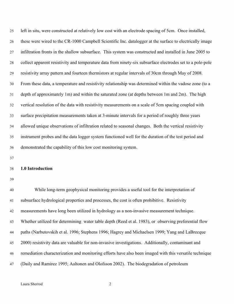
determined following the procedure outlined by Gronki and Sauck (2000). Figure 1 shows an example 86
of a finished ρa and temperature probe. 87
Laura Sherrod 5
88
Figure 1: Resistivity and temperature probe with electrode spacing of 5cm and thermistors spaced at 30 89
cm. 90
Electronic Instrument System Design 91
To achieve our low-cost objective, the assemblage of the acquisition and datalogging system 92
from off-the-shelf components was required. The cost of materials for this project was $7400 and probe 93
construction required approximately forty hours. Commercially available resistivity meters do not 94
contain cost effective components necessary for long-term (i.e., longer than one year) experiments. 95
Laura Sherrod 6
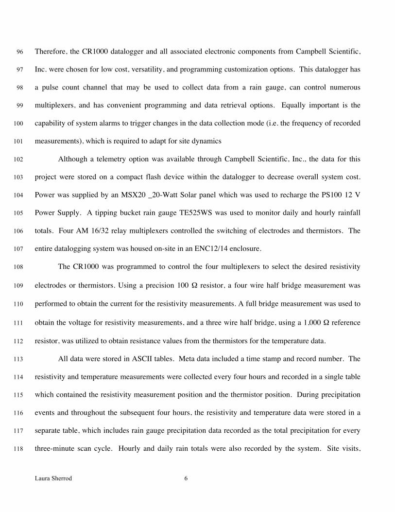
Therefore, the CR1000 datalogger and all associated electronic components from Campbell Scientific, 96
Inc. were chosen for low cost, versatility, and programming customization options. This datalogger has 97
a pulse count channel that may be used to collect data from a rain gauge, can control numerous 98
multiplexers, and has convenient programming and data retrieval options. Equally important is the 99
capability of system alarms to trigger changes in the data collection mode (i.e. the frequency of recorded 100
measurements), which is required to adapt for site dynamics 101
Although a telemetry option was available through Campbell Scientific, Inc., the data for this 102
project were stored on a compact flash device within the datalogger to decrease overall system cost. 103
Power was supplied by an MSX20 _20-Watt Solar panel which was used to recharge the PS100 12 V 104
Power Supply. A tipping bucket rain gauge TE525WS was used to monitor daily and hourly rainfall 105
totals. Four AM 16/32 relay multiplexers controlled the switching of electrodes and thermistors. The 106
entire datalogging system was housed on-site in an ENC12/14 enclosure. 107
The CR1000 was programmed to control the four multiplexers to select the desired resistivity 108
electrodes or thermistors. Using a precision 100 Ω resistor, a four wire half bridge measurement was 109
performed to obtain the current for the resistivity measurements. A full bridge measurement was used to 110
obtain the voltage for resistivity measurements, and a three wire half bridge, using a 1,000 Ω reference 111
resistor, was utilized to obtain resistance values from the thermistors for the temperature data. 112
All data were stored in ASCII tables. Meta data included a time stamp and record number. The 113
resistivity and temperature measurements were collected every four hours and recorded in a single table 114
which contained the resistivity measurement position and the thermistor position. During precipitation 115
events and throughout the subsequent four hours, the resistivity and temperature data were stored in a 116
separate table, which includes rain gauge precipitation data recorded as the total precipitation for every 117
three-minute scan cycle. Hourly and daily rain totals were also recorded by the system. Site visits, 118

Laura Sherrod 7
varying in frequency from once every few days to several months, were made to retrieve the data from 119
the compact flash card and for system inspection. 120
Due to the depth to the water table and constraints with the datalogger capacity, the most 121
practical design for experimental testing of this system was four individual probes; two of one-meter 122
length and two of two-meter length. Probes 1 and 2 each contained sixteen electrodes. Probe 3 123
contained thirty-one electrodes and Probe 4 contained thirty-three electrodes. These lengths ensured that 124
each probe crossed the transition between the vadose and saturated zones. The datalogger was 125
connected to the probes and configured to record a series of Pole-Pole resistivity measurements from 126
adjacent electrodes on the same probe which resulted in ninety-two measurement positions every four 127
hours. Due to constraints of the data logging system and chosen multiplexers, not all possible 128
combinations of electrode pairs on a given vertical array were used. Resistivity measurements were 129
only taken from electrodes adjacent to each other on the same probe. During precipitation events and 130
for the next four hours following such events, the frequency of the data collection cycle was increased to 131
one cycle every three minutes. These data provided a very detailed image of infiltration events. 132
Field Site 133
The test site was in a hay field near a man-made pond constructed approximately fifty years ago 134
in Pine Grove Township (Township 1 South, Range 13 West), Van Buren County, Michigan. The 135
probes were installed vertically into the subsurface at an increasing distance from the pond and in a line 136
perpendicular to the bank of the pond (Figure 2). Surface resistivity and ground penetrating radar (GPR) 137
surveys along perpendicular lines verified the lateral continuity of soil layers prior to probe installation. 138
When the pond was created, the excavated material was piled on top of the soil surface surrounding the 139
new pond. A 5-cm (2-inch) diameter monitoring well was installed 0.5 m from each probe at the same 140
distance from the pond to monitor water table levels at periodic intervals throughout the experiment. A 141

Laura Sherrod 8
time domain reflectometry (TDR) access tube was installed 0.5 m near each probe. Unfortunately, a 142
necessary deviation from the recommended installation procedure for the access tube, due to the 143
presence of large pebbles and cobbles, invalidated most of the TDR results and thus those are not 144
presented. Additional attempts through the use of a neutron probe to obtain moisture content data also 145
failed due to the inhomogeneities of the subsurface. As such, a qualitative measure of the subsurface 146
moisture content was performed. Probes 1, 2, 3, and 4 were installed in a row perpendicular to the pond, 147
at 3 m, 4 m, 6 m, and 9 m from the edge of the water at the time of installation. The water level of the 148
pond was below 230 m (+/- 1 m) elevation throughout the duration of the experiment. 149
Laura Sherrod 9
150
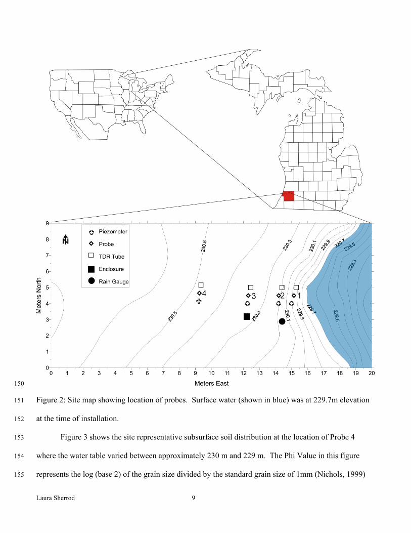
Figure 2: Site map showing location of probes. Surface water (shown in blue) was at 229.7m elevation 151
at the time of installation. 152
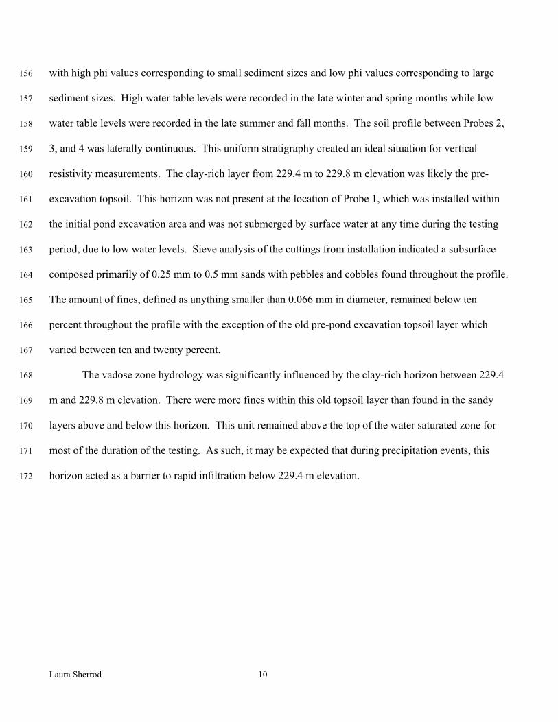
Figure 3 shows the site representative subsurface soil distribution at the location of Probe 4 153
where the water table varied between approximately 230 m and 229 m. The Phi Value in this figure 154
represents the log (base 2) of the grain size divided by the standard grain size of 1mm (Nichols, 1999) 155
Laura Sherrod 10
with high phi values corresponding to small sediment sizes and low phi values corresponding to large 156
sediment sizes. High water table levels were recorded in the late winter and spring months while low 157
water table levels were recorded in the late summer and fall months. The soil profile between Probes 2, 158
3, and 4 was laterally continuous. This uniform stratigraphy created an ideal situation for vertical 159
resistivity measurements. The clay-rich layer from 229.4 m to 229.8 m elevation was likely the pre-160
excavation topsoil. This horizon was not present at the location of Probe 1, which was installed within 161
the initial pond excavation area and was not submerged by surface water at any time during the testing 162
period, due to low water levels. Sieve analysis of the cuttings from installation indicated a subsurface 163
composed primarily of 0.25 mm to 0.5 mm sands with pebbles and cobbles found throughout the profile. 164
The amount of fines, defined as anything smaller than 0.066 mm in diameter, remained below ten 165
percent throughout the profile with the exception of the old pre-pond excavation topsoil layer which 166
varied between ten and twenty percent. 167
The vadose zone hydrology was significantly influenced by the clay-rich horizon between 229.4 168
m and 229.8 m elevation. There were more fines within this old topsoil layer than found in the sandy 169
layers above and below this horizon. This unit remained above the top of the water saturated zone for 170
most of the duration of the testing. As such, it may be expected that during precipitation events, this 171
horizon acted as a barrier to rapid infiltration below 229.4 m elevation. 172
Laura Sherrod 11
173
Figure 3: Lithologic description of the five distinct geologic units as observed at the location of Probe 4. 174
These units are similar for the other probe locations. 175
228.6
228.8
229
229.2
229.4
229.6
229.8
230
230.2
230.4
0 Elapsed Time (min)
Ele
vatio
n (m
eter
s)
2-Jan-0613-Jan-0628-Jan-068-Mar-067-Apr-06
230.30
0
10
20
30
40
-1 0 1 2 3 4 5
228.93
0
10
20
30
40
-1 0 1 2 3 4 5
229.99
0
10
20
30
40
-1 0 1 2 3 4 5
229.69
0
10
20
30
40
-1 0 1 2 3 4 5
229.08
0
10
20
30
40
-1 0 1 2 3 4 5
Brown to Black, Fine to Medium Grained Sandwith organics and small amounts of clay (topsoil)
Brown, Medium Grained Sand with organics,cobbles and/or pebbles, and small amounts of clay
Black, Organic-rich with Medium Grained Sandand significant amounts of clay
Brown, Fine Grained Sand with pebbles
Red, Medium Grained Sandwith cobbles and/or pebbles
0
5
10
15
20
25
30
01-Nov-06 16-Nov-06 01-Dec-06 16-Dec-06 31-Dec-06 15-Jan-07
Date
Dai
ly R
ain
(mm
)
228.6
228.8
229.0
229.2
229.4
229.6
229.8
230.0
230.2
230.4
Elev
atio
n (m
eter
s)
Percent ChangeResistivity 25 to 30 15 to 60 10 to 15 5 to 10 0 to 5 -5 to 0 -10 to -5 -15 to -10 -20 to -15 -100 to -20
Brown to Black, Fine to Medium Grained Sandwith organics and small amounts of clay (topsoil)
Brown, Medium Grained Sand with organics,cobbles and/or pebbles, and small amounts of clay
Black, Organic-rich with Medium Grained Sand and significant amounts of clay
Brown, Fine Grained Sand with pebbles
Red, Medium Grained Sand with cobbles and/or pebbles
Phi value (φ)
Perc
ent (
%)
Perc
ent (
%)
Perc
ent (
%)
Perc
ent (
%)
Perc
ent (
%)Phi value (φ)
Phi value (φ)
Phi value (φ)
Phi value (φ)
Laura Sherrod 12
176
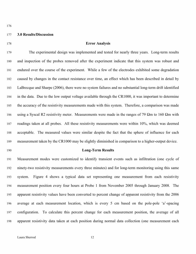
3.0 Results/Discussion 177
Error Analysis 178
The experimental design was implemented and tested for nearly three years. Long-term results 179
and inspection of the probes removed after the experiment indicate that this system was robust and 180
endured over the course of the experiment. While a few of the electrodes exhibited some degradation 181
caused by changes in the contact resistance over time, an effect which has been described in detail by 182
LaBrecque and Sharpe (2006), there were no system failures and no substantial long-term drift identified 183
in the data. Due to the low output voltage available through the CR1000, it was important to determine 184
the accuracy of the resistivity measurements made with this system. Therefore, a comparison was made 185
using a Syscal R2 resistivity meter. Measurements were made in the ranges of 79 Ωm to 160 Ωm with 186
readings taken at all probes. All these resistivity measurements were within 10%, which was deemed 187
acceptable. The measured values were similar despite the fact that the sphere of influence for each 188
measurement taken by the CR1000 may be slightly diminished in comparison to a higher-output device. 189
Long-Term Results 190
Measurement modes were customized to identify transient events such as infiltration (one cycle of 191
ninety-two resistivity measurements every three minutes) and for long-term monitoring using this same 192
system. Figure 4 shows a typical data set representing one measurement from each resistivity 193
measurement position every four hours at Probe 1 from November 2005 through January 2008. The 194
apparent resistivity values have been converted to percent change of apparent resistivity from the 2006 195
average at each measurement location, which is every 5 cm based on the pole-pole ‘a’-spacing 196
configuration. To calculate this percent change for each measurement position, the average of all 197
apparent resistivity data taken at each position during normal data collection (one measurement each 198
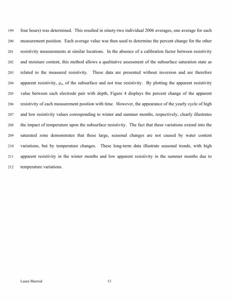
Laura Sherrod 13
four hours) was determined. This resulted in ninety-two individual 2006 averages, one average for each 199
measurement position. Each average value was then used to determine the percent change for the other 200
resistivity measurements at similar locations. In the absence of a calibration factor between resistivity 201
and moisture content, this method allows a qualitative assessment of the subsurface saturation state as 202
related to the measured resistivity. These data are presented without inversion and are therefore 203
apparent resistivity, ρa, of the subsurface and not true resistivity. By plotting the apparent resistivity 204
value between each electrode pair with depth, Figure 4 displays the percent change of the apparent 205
resistivity of each measurement position with time. However, the appearance of the yearly cycle of high 206
and low resistivity values corresponding to winter and summer months, respectively, clearly illustrates 207
the impact of temperature upon the subsurface resistivity. The fact that these variations extend into the 208
saturated zone demonstrates that these large, seasonal changes are not caused by water content 209
variations, but by temperature changes. These long-term data illustrate seasonal trends, with high 210
apparent resistivity in the winter months and low apparent resistivity in the summer months due to 211
temperature variations. 212
Laura Sherrod 14
213
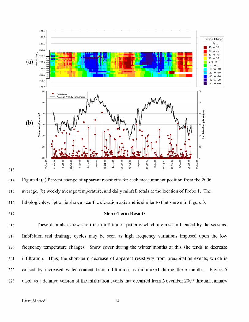
Figure 4: (a) Percent change of apparent resistivity for each measurement position from the 2006 214
average, (b) weekly average temperature, and daily rainfall totals at the location of Probe 1. The 215
lithologic description is shown near the elevation axis and is similar to that shown in Figure 3. 216
Short-Term Results 217
These data also show short term infiltration patterns which are also influenced by the seasons. 218
Imbibition and drainage cycles may be seen as high frequency variations imposed upon the low 219
frequency temperature changes. Snow cover during the winter months at this site tends to decrease 220
infiltration. Thus, the short-term decrease of apparent resistivity from precipitation events, which is 221
caused by increased water content from infiltration, is minimized during these months. Figure 5 222
displays a detailed version of the infiltration events that occurred from November 2007 through January 223
228.6
228.8
229.0
229.2
229.4
229.6
229.8
230.0
230.2
230.4
Elev
atio
n (m
)Percent Change
Resistivity 45 to 70 30 to 45 20 to 30 10 to 20 0 to 10 -10 to 0 -15 to -10 -20 to -15 -30 to -20 -40 to -30 -55 to -40
-30
-20
-10
0
10
20
30
30-S
ep-0
5
19-N
ov-0
5
8-Ja
n-06
27-F
eb-0
6
18-A
pr-0
6
7-Ju
n-06
27-J
ul-0
6
15-S
ep-0
6
4-N
ov-0
6
24-D
ec-0
6
12-F
eb-0
7
3-Ap
r-07
23-M
ay-0
7
12-J
ul-0
7
31-A
ug-0
7
20-O
ct-0
7
9-D
ec-0
7
28-J
an-0
8
18-M
ar-0
8
Tem
pera
ture
(deg
rees
C)
0
10
20
30
40
50
60
Cum
ulat
ive
Prec
ipita
tion
(mm
)
Daily Rain42 per. Mov. Avg. (Temp)Daily RainAverage Weekly Temperature
Percent Changeρa
(a)
(b)

Laura Sherrod 15
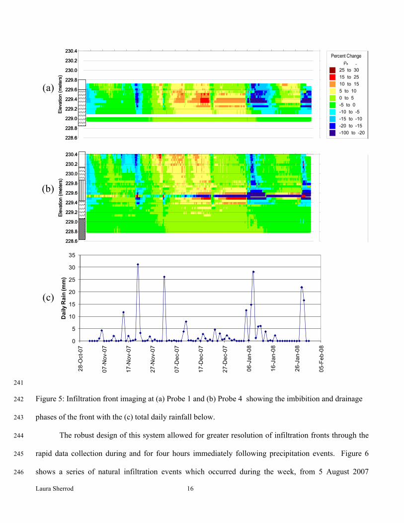
2008 at Probe 1 and Probe 4. These data also reveal a faulty electrode connection apparent at 229.5m 224
elevation at Probe 4. Nevertheless, the overall subsurface apparent resistivity changes are clearly 225
evident. It is clear (Figure 5) that the stratigraphic unit with abundant fines at 229.4m to 228.8m 226
elevation is a significant contributor to subsurface water flow. This is evident through the increased 227
time that this unit maintains a lower apparent resistivity (i.e. the fines are holding on to the water that 228
has infiltrated) compared to the upper unit which allows more rapid infiltration. An example of this may 229
be seen in Figure 5 on 2 December 2007 when there was a precipitation event of over 26mm. The 230
decreased apparent resistivity within the clay-rich unit persists for nearly four days following the 231
precipitation event while the upper unit returns to higher apparent resistivity values by the next day after 232
the precipitation. 233
It should be noted that the air temperature during the first half of the month of January 2008 was 234
abnormally high, allowing for several infiltration events to occur in response to rainfall and snow melt. 235
Overall, the impact of infiltration on the subsurface is subdued during the winter months, as seen in 236
December 2007, due to the frozen ground surface and snow cover restricting infiltration. The data 237
collection method of this system allows a visualization of surface temperature’s influence upon the 238
amount of infiltration. Figure 5 illustrates the impact and extent of precipitation events from 5-13 239
January and 28-29 January impacting the subsurface water content 240
Laura Sherrod 16
241
Figure 5: Infiltration front imaging at (a) Probe 1 and (b) Probe 4 showing the imbibition and drainage 242
phases of the front with the (c) total daily rainfall below. 243
The robust design of this system allowed for greater resolution of infiltration fronts through the 244
rapid data collection during and for four hours immediately following precipitation events. Figure 6 245
shows a series of natural infiltration events which occurred during the week, from 5 August 2007 246
0
5
10
15
20
25
30
35
28-O
ct-0
7
07-N
ov-0
7
17-N
ov-0
7
27-N
ov-0
7
07-D
ec-0
7
17-D
ec-0
7
27-D
ec-0
7
06-J
an-0
8
16-J
an-0
8
26-J
an-0
8
05-F
eb-0
8
Dai
ly R
ain
(mm
)
228.6
228.8
229.0
229.2
229.4
229.6
229.8
230.0
230.2
230.4
Elev
atio
n (m
eter
s)Percent Change
Resistivity
25 to 30 15 to 25 10 to 15 5 to 10 0 to 5 -5 to 0 -10 to -5 -15 to -10 -20 to -15 -100 to -20
228.6
228.8
229.0
229.2
229.4
229.6
229.8
230.0
230.2
230.4
Elev
atio
n (m
eter
s)Percent Change
Resistivity
25 to 30 15 to 25 10 to 15 5 to 10 0 to 5 -5 to 0 -10 to -5 -15 to -10 -20 to -15 -100 to -20
0
5
10
15
20
25
30
35
28-O
ct-0
7
07-N
ov-0
7
17-N
ov-0
7
27-N
ov-0
7
07-D
ec-0
7
17-D
ec-0
7
27-D
ec-0
7
06-J
an-0
8
16-J
an-0
8
26-J
an-0
8
05-F
eb-0
8
Dai
ly R
ain
(mm
)
228.6
228.8
229.0
229.2
229.4
229.6
229.8
230.0
230.2
230.4
Elev
atio
n (m
eter
s)
Percent ChangeResistivity
25 to 30 15 to 25 10 to 15 5 to 10 0 to 5 -5 to 0 -10 to -5 -15 to -10 -20 to -15 -100 to -20
228.6
228.8
229.0
229.2
229.4
229.6
229.8
230.0
230.2
230.4
Elev
atio
n (m
eter
s)
Percent ChangeResistivity
25 to 30 15 to 25 10 to 15 5 to 10 0 to 5 -5 to 0 -10 to -5 -15 to -10 -20 to -15 -100 to -20
Percent Changeρa
(a)
(b)
(c)
Laura Sherrod 17
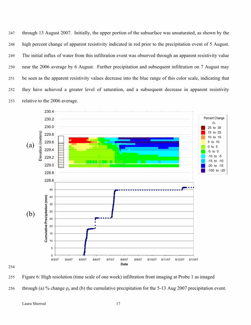
through 13 August 2007. Initially, the upper portion of the subsurface was unsaturated, as shown by the 247
high percent change of apparent resistivity indicated in red prior to the precipitation event of 5 August. 248
The initial influx of water from this infiltration event was observed through an apparent resistivity value 249
near the 2006 average by 6 August. Further precipitation and subsequent infiltration on 7 August may 250
be seen as the apparent resistivity values decrease into the blue range of this color scale, indicating that 251
they have achieved a greater level of saturation, and a subsequent decrease in apparent resistivity 252
relative to the 2006 average. 253
254
Figure 6: High resolution (time scale of one week) infiltration front imaging at Probe 1 as imaged 255
through (a) % change ρa and (b) the cumulative precipitation for the 5-13 Aug 2007 precipitation event. 256
0
5
10
15
20
25
30
35
40
45
50
8/3/07 8/4/07 8/5/07 8/6/07 8/7/07 8/8/07 8/9/07 8/10/07 8/11/07 8/12/07 8/13/07
Cum
ulat
ive
Prec
ipita
tion
(mm
)
Date
228.6
228.8
229.0
229.2
229.4
229.6
229.8
230.0
230.2
230.4
Elev
atio
n (m
eter
s)
Percent ChangeResistivity
25 to 30 15 to 60 10 to 15 5 to 10 0 to 5 -5 to 0 -10 to -5 -15 to -10 -20 to -15 -100 to -20228.6
228.8
229.0
229.2
229.4
229.6
229.8
230.0
230.2
230.4
Elev
atio
n (m
eter
s)
Percent ChangeResistivity
25 to 30 15 to 25 10 to 15 5 to 10 0 to 5 -5 to 0 -10 to -5 -15 to -10 -20 to -15 -100 to -20
228.6
228.8
229.0
229.2
229.4
229.6
229.8
230.0
230.2
230.4
Elev
atio
n (m
eter
s)
Percent ChangeResistivity
25 to 30 15 to 25 10 to 15 5 to 10 0 to 5 -5 to 0 -10 to -5 -15 to -10 -20 to -15 -100 to -20
Percent Changeρa
(a)
(b)
Laura Sherrod 18
Temperature Dependence 257
There is an obvious correlation between the weekly average temperature and the measured 258
apparent resistivity in Figure 4, which is expected since temperature influences apparent resistivity. 259
Apparent resistivity decreases during the summer months due to increased temperatures and increases 260
during the winter months due to decreased temperatures. Keller and Frischknecht (1966) indicate 261
theoretical temperature dependency of electrolyte or rock saturated with electrolyte in the following 262
formula: 263
𝜌! =𝜌!"
1+ 𝛼!(𝑡 − 18°)
where ρ18 is the reference resistivity at 18⁰C (although other temperatures may be used), αt is the 264
temperature coefficient of resistivity (typically 0.025/⁰C), t is the changed temperature, and ρt is the 265
resistivity at the changed temperature. This work was advanced in low-temperature geologic 266
environments, within the range of 0-25⁰C, by Hayley et al. (2007). These researchers performed 267
laboratory experiments and a field study showing a 1.8% to 2.2% change in the bulk electrical 268
conductivity per degree Celsius, which should be considered a representative approximation, in the 269
absence of other information (Hayley et al., 2007). Using a reference resistivity of 160Ωm at 18⁰C and 270
solving for the resistivity at 8⁰C using the formula presented by Keller and Frischknecht, a percent 271
change in the electrical conductivity of 2.5% per degree Celsius is obtained. The above reference 272
resistivity and temperature values were chosen because they fall within the range of data collected at our 273
field site. 274
We tested these approximations by selecting reference values from our vadose zone and 275
saturated zone data and determined empirical temperature coefficients for these two zones. A sample of 276
data was taken between 5 March 2007 and 28 May 2007, which consisted of a total of 500 data points 277
from the normal data collection mode, to derive an empirical relationship between the temperature and 278
Laura Sherrod 19
the bulk electrical conductivity at the location of Probe 1. Our empirically derived relationship using 279
subsurface temperatures measured by the probe thermistors shows a 2.98% change of conductivity per 280
degree Celsius in the saturated zone and a 5.27% change of conductivity per degree Celsius in the 281
vadose zone. Recall, these percent changes were calculated with respect to the apparent resistivity 282
measured on 13 May 2007. This date was chosen because a measurement of the pore water conductivity 283
was made on this date. The saturated zone response was determined from data at the lowest five 284
measurement positions. The unsaturated zone response was determined from the data collected at the 285
upper six measurement positions. This temperature correction was applied to the apparent resistivity 286
values of Probe 1 between December 2006 and August 2007. 287
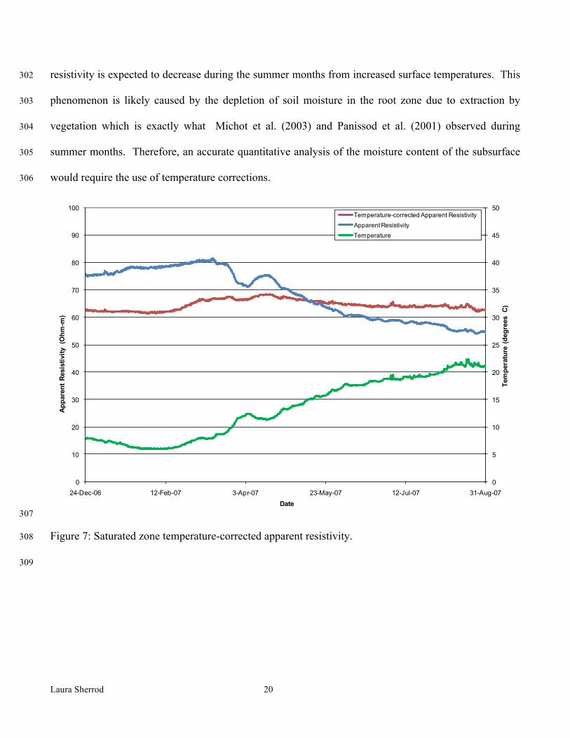
Apparent resistivity values from 228.98 m elevation at the location of Probe 1 from 24 December 288
2006 through 31 August 2007 were corrected for temperature and are displayed in Figure 7. The 289
measurement position shown in this figure remained below the water table for the duration of the time 290
range plotted. As such it may be assumed that the apparent resistivity was not impacted by saturation 291
changes. The most likely changes at this position would be caused by changes in temperature or pore 292
water conductivity variations. At this elevation of Probe 1, the overall range of temperature-corrected 293
apparent resistivity observed between 24 December 2006 and 31 August 2007 is 61.42 Ωm to 68.49 294
Ωm. As the overall apparent resistivity at this position remains fairly constant, we assume that the pore 295
water conductivity does not significantly vary over the sampled time interval. Figure 8 shows similar 296
results at an elevation of 229.63 m at Probe 1 and depicts measurements made in the vadose zone. The 297
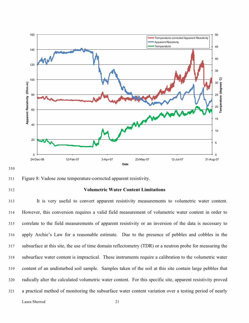
temperature-corrected apparent resistivity is influenced by the variation of vadose zone water content. 298
Thus interpretations concerning the saturation state of the subsurface may be made from Figure 8. 299
Interestingly, a marked increase of apparent resistivity is noted in June and July when the 300
apparent resistivity is corrected for temperature variations (Figure 8), despite the fact that the apparent 301
Laura Sherrod 20
resistivity is expected to decrease during the summer months from increased surface temperatures. This 302
phenomenon is likely caused by the depletion of soil moisture in the root zone due to extraction by 303
vegetation which is exactly what Michot et al. (2003) and Panissod et al. (2001) observed during 304
summer months. Therefore, an accurate quantitative analysis of the moisture content of the subsurface 305
would require the use of temperature corrections. 306
307
Figure 7: Saturated zone temperature-corrected apparent resistivity. 308
309
0
5
10
15
20
25
30
35
40
45
50
0
10
20
30
40
50
60
70
80
90
100
24-Dec-06 12-Feb-07 3-Apr-07 23-May-07 12-Jul-07 31-Aug-07
Tem
pera
ture
(deg
rees
C)
Appa
rent
Res
istiv
ity (
Ohm
-m)
Date
Temperature-corrected Apparent ResistivityApparent ResistivityTemperature
Laura Sherrod 21
310
Figure 8: Vadose zone temperature-corrected apparent resistivity. 311
Volumetric Water Content Limitations 312
It is very useful to convert apparent resistivity measurements to volumetric water content. 313
However, this conversion requires a valid field measurement of volumetric water content in order to 314
correlate to the field measurements of apparent resistivity or an inversion of the data is necessary to 315
apply Archie’s Law for a reasonable estimate. Due to the presence of pebbles and cobbles in the 316
subsurface at this site, the use of time domain reflectometry (TDR) or a neutron probe for measuring the 317
subsurface water content is impractical. These instruments require a calibration to the volumetric water 318
content of an undisturbed soil sample. Samples taken of the soil at this site contain large pebbles that 319
radically alter the calculated volumetric water content. For this specific site, apparent resistivity proved 320
a practical method of monitoring the subsurface water content variation over a testing period of nearly 321
0
5
10
15
20
25
30
35
40
45
50
0
20
40
60
80
100
120
140
160
24-Dec-06 12-Feb-07 3-Apr-07 23-May-07 12-Jul-07 31-Aug-07
Tem
pera
ture
(deg
rees
C)
Appa
rent
Res
istiv
ity (
Ohm
-m)
Date
Temperature-corrected Apparent ResistivityApparent ResistivityTemperature
Laura Sherrod 22
three years. A general understanding of the water content may be obtained in heterogeneous subsurfaces 322
such as the one encountered at this site through the use of the resistivity index, which is defined as the 323
observed resistivity divided by the saturated resistivity. However, this requires foreknowledge of the 324
resistivity at saturation for each measurement position. Alternatively, as shown in this work, the percent 325
change of apparent resistivity can be used to qualitatively image the saturation state of the subsurface in 326
the absence of a true calibration between volumetric water content and resistivity. 327
328
4.0 Conclusions 329
330
The method presented in this work details an example of a low-cost system of making long-term 331
subsurface apparent resistivity and temperature measurements in a shallow field setting. The system 332
contains low-cost commercially available components and proved durable over the course of nearly 333
three years. High quality, high resolution data were collected at a moderately heterogeneous, shallow 334
subsurface location. The electrode spacing of 5 cm allowed an intricate depiction of the infiltration of 335
precipitation in a natural field setting, while the durable nature of the system allowed long-term 336
observations. The short-term, high temporal resolution, data collection during and after precipitation 337
events clearly shows imbibition and drainage due to natural infiltration events. Seasonal trends are 338
observed in the long-term apparent resistivity data as temperature variations, with high apparent 339
resistivity values in the winter months and low apparent resistivity values in the summer months, and 340
infiltration patterns, which are influenced by the seasonal variation in precipitation form (rain versus 341
snow) and ground cover (grass versus snow). Subsurface temperature variability impacted field 342
resistivity measurements, especially over long time periods. At the field site analyzed in this study, the 343
variation of conductivity with temperature was a 2.97% increase of conductivity per degree Celsius in 344
the saturated zone and a 5.27% increase of conductivity per degree Celsius in the vadose zone. 345
Laura Sherrod 23
Apparent resistivity has been shown to monitor infiltration fronts and to identify water uptake by plant 346
roots. As an extension to the applicability of this system, resistivity could, in some circumstances, be 347
used to determine useful hydrogeological parameters such as water content in the vadose zone, but only 348
if resistivity can be previously calibrated against absolute water content at the same site. Likewise, the 349
low-cost system described herein could be applied to low-budget projects which may require the 350
monitoring of either subsurface water content or chemical changes of subsurface water which may be 351
correlated to resistivity changes and possible agricultural studies of plant water uptake. 352
353
5.0 Acknowledgements 354
355
Funding for this project was provided by the Michigan Space Grant Consortium Graduate Research 356
Fellowship. The authors wish to thank Mr. Rockie Keeley for the use of his land as a field test site. 357
Although this work was reviewed by EPA and approved for presentation, it may not necessarily reflect 358
official Agency policy. Mention of trade names or commercial products does not constitute 359
endorsement or recommendation by EPA for use. We also appreciate the comments from reviewers, 360
which strengthened and clarified this manuscript. 361
362
References 363
Aaltonen, J. and B. Olofsson. 2002. Direct current (DC) resistivity measurements in long-term 364
groundwater monitoring programmes. Environmental Geology, 41(6): 662-671. 365
Atekwana, E.A., W.A. Sauck, and D.D. Werkema, Jr. 2000. Investigations of geoelectrical signatures at 366
a hydrocarbon contaminated site. Journal of Applied Geophysics, 44: 167-180. 367
Laura Sherrod 24
Binley, A., G. Cassiani, R. Middleton, and P. Winship. 2002a. Vadose zone flow model 368
parameterisation using cross-borehole radar and resistivity imaging. Journal of Hydrology, 267: 369
147-159. 370
Binley, A., P. Winship, L.J. West, M. Pokar, and R. Middleton. 2002b. Seasonal variation of moisture 371
content in unsaturated sandstone inferred from borehole radar and resistivity profiles. Journal of 372
Hydrology, 267: 160-172. 373
Cassiani, G., V. Bruno, A. Villa, N. Fusi, and A.M. Binley. 2006. A saline trace test monitored via time-374
lapse surface electrical resistivity tomography. Journal of Applied Geophysics, 59: 244-259. 375
Daily, W. and A. Ramirez. 1995. Electrical resistance tomography during in-situ trichloroethylene 376
remediation at the Savannah River Site. Journal of Applied Geophysics, 33: 239-249. 377
Grimm, R.E., G.R. Olhoeft, K. McKinley, J. Rossabi, and B. Riha. 2005. Nonlinear Complex-Resistivity 378
Survey for DNAPL at the Savannah River Site A-014 Outfall. Journal of Environmental and 379
Engineering Geophysics, 10(4): 351-364. 380
Groncki, J.M. and W.A. Sauck. 2000. Calibration, installation techniques, and equilibration 381
considerations for vertical resistivity probes used in hydrogeologic investigations, Symposium 382
on the Application of Geophysics to Engineering and Environmental Problems, pp. 979-988. 383
Hagrey, S.A. and J. Michaelsen. 1999. Resistivity and percolation study of preferential flow in vadose 384
zone at Bokhorst, Germany. Geophysics, 64(3): 746-753. 385
Hayley, K., L. Bentley, M. Gharibi, and M. Nightingale. 2007. Low temperature dependence of 386
electrical resistivity: Implications for near surface geophysical monitoring. Geophysical 387
Research Letters, 34: L18402. 388
Laura Sherrod 25
Johnson, T., R. Versteeg, H. Huang, and P. Routh. 2009. Data-domain correlation approach for joint 389
hydrogeologic inversion of time-lapse hydrogeologic and geophysical data. Geophysics. 74: 390
F127-F140. 391
Keller and Frischknecht. 1966. Electrical Methods in Geophysical Prospecting. Oxford: Pergamon 392
Press. 393
Kemna, A., J. Vanderborght, B. Kulessa, and H. Vereecken. 2002. Imaging and characterisation of 394
subsurface solute transport using electrical resistivity tomography (ERT) and equivalent 395
transport models. Journal of Hydrology, 267: 125-146. 396
LaBrecque, D. and W. Daily. 2008. Assessment of measurement errors for galvanic-resistivity 397
electrodes of different composition. Geophysics, 73(2): F55-F64. 398
LaBrecque, D. and R. Sharpe. 2006. Progress in Ultra-High Precision Resistivity Tomography: 399
Electrode Aging in Long-Term Monitoring. Symposium on the Application of Geophysics to 400
Engineering and Environmental Problems, pp. 639-646. 401
Linde, N., A. Binley, A. Tryggvason, L.B. Pedersen, and A. Revil. 2006. Improved hydrogeophysical 402
characterization using joint inversion of cross-hole electrical resistance and ground-penetrating 403
radar traveltime data. Water Resources Research, 42: W12404. 404
Michot, D., Y. Benderitter, A. Dorigny, B. Nicoullaud, D. King, and A. Tabbagh. 2003. Spatial and 405
temporal monitoring of soil water content with an irrigated corn crop cover using surface 406
electrical resistivity tomography. Water Resources Research, 39(5): 14-1 - 14-20. 407
Narbutovskih, S.M., W. Daily, A.L. Ramirez, T.D. Halter, and M.D. Sweeney. 1996. Electrical 408
resistivity tomography at the DOE Hanford site, Symposium on the Application of Geophysics to 409
Engineering and Environmental Problems, pp. 773-782. 410
Nichols, G. 1999. Sedimentology & Stratigraphy: Cambridge, University Press, 355 p. 411
Laura Sherrod 26
Ogilvy, R., P. Meldrum, O. Kura, P. Wilkinson, J. Chambers, M. Sen, A. Pulido-Bosch, J. Gisbert, S. 412
Jorreto, I. Frances, and P. Tsourlos. 2009. Automated monitoring of coastal aquifers with 413
electrical resistivity tomography. Near Surface Geophysics, 7: 367-375. 414
Panissod, C., D. Michot, Y. Benderitter, and A. Tabbagh. 2001. On the effectiveness of 2D electrical 415
inversion results: an agricultural case study. Geophysical Prospecting, 49: 570-576. 416
Pfiefer, M.C. and H.T. Andersen. 1995. DC-resistivity array to monitor fluid flow at the INEL 417
infiltration test, Symposium on the Application of Geophysics to Engineering and Environmental 418
Problems, pp. 709-718. 419
Reed, P.C., P.B. DuMontelle, M.L. Sargent, and M.M. Killey. 1983. Nuclear Logging and Electrical 420
Earth Resistivity Techniques in the Vadose Zone in Glaciated Earth Materials, NWWA/U.S. 421
EPA conference on characterization and monitoring of the vadose (unsaturated) zone, pp. 580-422
601. 423
Sauck, W.A. 2000. A model for the resistivity structure of LNAPL plumes and their environs in sandy 424
sediments. Journal of Applied Geophysics, 44: 151-165. 425
Singha, K. and S. Gorelick. 2005. Saline tracer visualized with three-dimensional electrical resistivity 426
tomography: Field-scale spatial moment analysis. Water Resources Research, 41: W05023. 427
Singha, K. and S. Gorelick. 2006a. Effects of spatially variable resolution on field-scale estimates of 428
tracer concentration from electrical inversions using Archie's law. Geophysics, 71(3): G83-G91. 429
Singha, K. and S. Gorelick. 2006b. Hydrogeophysical tracking of three-dimensional tracer migration: 430
The concept and application of apparent petrophysical relations. Water Resources Research, 42: 431
W06422. 432
Stephens, D.B. 1996. Vadose Zone Hydrology. Boca Raton, FL: CRC Press, Inc. 433
Laura Sherrod 27
Vanderborght, J., A. Kemna, H. Hardelauf, and H. Vereecken. 2005. Potential of electrical resistivity 434
tomography to infer aquifer transport characteristics from tracer studies: A synthetic case study. 435
Water Resources Research, 41: W06013. 436
Werkema, D. 2002. Geoelectrical Response of an Aged LNAPL Plume: Implications for Monitoring 437
Natural Attenuation. Ph.D. diss., Department of Geology, Western Michigan University. 438
Werkema, D.D., E.A. Atekwana, E.A. Atekwana, J. Duris, J. Allen, L. Smart, and W.A. Sauck. 2004. 439
Laboratory and field results linking high bulk conductivities to the microbial degradation of 440
petroleum hydrocarbons, Symposium on the Application of Geophysics to Engineering and 441
Environmental Problems, pp. 363-373. 442
Yang, X. and D. LaBrecque. 2000. Estimation of 3-D moisture content using ERT data at the Socorro-443
Tech Vadose Zone Facility, Symposium on the Application of Geophysics to Engineering and 444
Environmental Problems, pp. 915-924. 445
446