A Lumped Element Modeling Schema for Metabotropic Signaling in Neurons

Richard B. Wells

MRC Institute, The University of Idaho

Abstract: A lumped element modeling schema is presented that can be usefully applied to

modeling and analysis of metabotropic processes affecting the signal processing properties of

neurons. The schema is easily applied to qualitative models of such biochemical processes and

facilitates the development of differential equation descriptions. The state variables within the

model are applicable to augmenting and extending Hodgkin-Huxley-like models (H-H models) of

neuron dynamics.

I. Introduction

There is something to be said in favor of having a general and versatile modeling schema for

particle accumulation, transport, chemical reaction, and storage in the cell. A general schema is

an aid for transforming qualitative models into quantitative ones and for developing relationships

descriptive of more complex physiological processes. After all, if the Hodgkin-Huxley schema is

useful in part because it provides a guide for dealing with the complexities of voltage-gated-

channel (VGC) and ligand-gate-channel (LGC) signaling, is it not also likely that a similar

schema will prove useful for dealing with cellular biochemical signaling processes?

In this paper we resurrect and adapt to our purposes a modeling schema originally developed

by Linvill [Linvill and Gibbons, 1961, pp. 17-48] and extend it to application in neuroscience.

The Linvill model was developed to represent carrier transport, storage, and generation-

recombination phenomena in semiconductors in terms of carrier densities and current flows. This

method has not previously been applied to biological signaling processing models. After all, the

neuron is not a transistor or a diode. Nonetheless, with only a few minor adaptations of the Linvill

model, one can apply it as a schema for representing particle flux and concentration in the cell.

This section introduces the basic modeling elements and their mathematical description. The next

sections illustrate some of its potential applications.

1

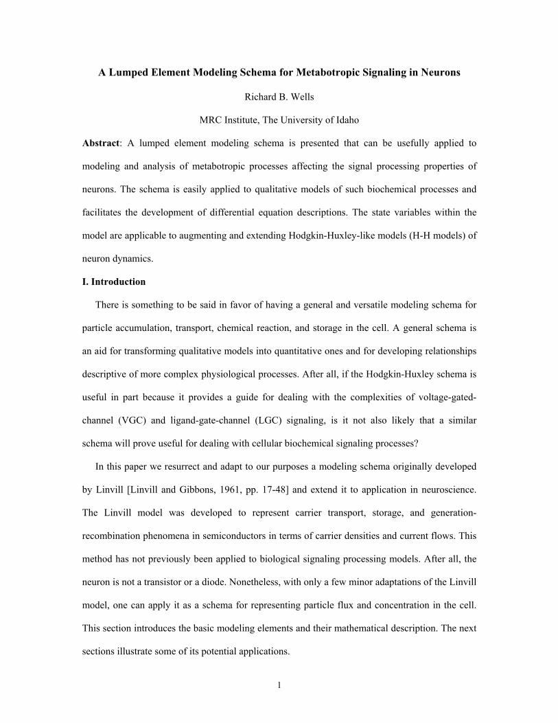
Figure 1: The five basic network elements of the Linvill modeling schema.

The Linvill modeling schema allows us to represent the model as a network of elements, each

of which is characterized by a specific element law. Figure 1 illustrates the five basic Linvill

network elements. Ion or molecule concentration is denoted by the symbol ν. Ion or molecule flux

is denoted by the symbol φ. Flux is positive in the direction denoted by the arrows. Particle (ion

or molecule) motion in space is formally describable in terms of partial differential equations with

boundary conditions. While such a description is mathematically rigorous and precise, it is also

rather cumbersome and computationally difficult to deal with in all but the simplest cases of

physical geometries. This issue is often overcome in the various sciences through the introduction

of the lumped element approximation. For example, electric and magnetic phenomena are

rigorously described by Maxwell’s equations, a set of partial differential equations. Circuit theory

is the lumped element approximation of these equations, applicable when electromagnetic

radiation (a consequence of Maxwell’s equations) is not an important factor. Similarly, the Linvill

model is a lumped element approximation to a partial differential equation description of particle

transport, storage, chemical reaction and accumulation processes.

The storage element ("storance") represents the accumulation of particles of a specific type in

a region due to influx from some other location or source. Its ν-φ relationship is based on the

mathematical form of the divergence theorem. The element law merely states that the net influx

of particles into the storage element is proportional to the time rate of change of concentration,

φνν==

∆&C

dtdC (1)

2

Dimensional analysis shows C has units of volume. C reflects the fact that a region of greater

volume builds up particle concentration less rapidly than a region of smaller volume for the same

amount of flux. We may at once note the similarity between (1) and the element law for a

capacitor in circuit theory. φ is analogous to electric current and ν is analogous to voltage. There

are, however, limits to this electric circuit analogy. The accumulation of ν in a storage element

does not induce the accumulation of some other particle elsewhere (no equivalent to charge on

one plate of a capacitor inducing the opposite charge on the other plate), and there is nothing

analogous to the displacement current through a capacitor, which is a consequence of Maxwell's

equations. Likewise, there is no "Kirchhoff’s voltage law" for this network. Particle flux is not

required to flow in a closed circuit path, hence the model is a network model rather than a circuit

model. Particle conservation, however, is required for the first four network elements because

only the reactance element represents a chemical reaction, e.g. a + b → c.

The flux source element represents influx/efflux from some exterior source. The most

common use for this element is to convert electric currents obtained from a H-H model to particle

flux. The current I due to a flux φ of particles with valence z is simply I = zeφ when φ is expressed

in particles per second. It is more convenient, however, to express flux in units such as

moles/second. In this case we would write I = zFφ, where F is Faraday’s constant. If we have a

current density – amperes per unit area – we replace flux by flux density. Letting β = 1/zF we

obtain the element law as φ = β⋅I with I in amperes and β in moles/coulomb. For z = 1, β is

numerically equal to 10.3643⋅10–6 moles/coulomb. Note that the sign of the valence is irrelevant

to flux (since this is merely the sign of the electric charge carried). Therefore if one is modeling

the flux of a negative-valence particle, the absolute value of z would be used.

The transporter symbol is a generalization of an element Linvill called a "combinance"

[Linvill, 1961, pg. 25]. In his original model this element was used to model charge generation

and recombination in semiconductors. That is a process by which bound charge is converted to

3

free charge and vice versa. The analog to this within the cell (not including chemical reactions

that produce new compounds) are processes by which free particles are introduced or removed by

various transport processes, such as the transport process by which free Ca2+ is removed from the

cytoplasm and stored in the endoplasmic reticulum [Hille, 2001, pp. 269-273]. In effect, these are

pumping processes in which the average flux is determined by the amount of particle transport

per cycle of the pump and the concentration of the particle being transported. Thus, the simplest

form of an element law for the transporter is the relationship

νρφ ⋅= (2)

where ρ is an empirically-determined transport parameter with units of volume/second. Note that

this expression is unidirectional. The concentration variable in (2) is placed at the "boxed" end of

the network element, and whatever the concentration may be at the other terminal is irrelevant.

The transporter does not represent a passive diffusion process. That dynamic is modeled by the

fourth network element.

The diffusion element ("diffusance") represents particle flux due to concentration differences.

Flux is positive in the direction from higher concentration to lower concentration. In its simplest

form, the diffusance element law is merely

( 21 )ννφ −⋅= D (3)

where D is an empirically-determined parameter with units of volume/second.

If C, ρ, and D are represented by simple constants we have a linear model of transport and

storage. Making these variables functions of ν, and possibly other variables, produces a nonlinear

model. At our present state of knowledge of neural metabotropic physiology no nonlinear model

of the neuron’s internal processes is in widespread use and, consequently, most computational

neuron modeling works have used linear models for most simple transport and storage processes.

This does not mean such models are correct; it merely reflects the state of knowledge one has.

Using the first four elements we can construct network models of arbitrary complexity to

4

represent various transport and storage processes excepting those involving chemical reactions.

Chemical reactions are modeled by the reactance element, which is discussed later in this paper.

If it happens to be the case where we do not care what happens later to these reaction products, a

derived element, called a reactor, combined with a storage element can suffice for representing

the introduction or the removal of free particles. This is also illustrated later. The next section

illustrates the application of this modeling schema to Ca2+ augmentation of the basic H-H model.

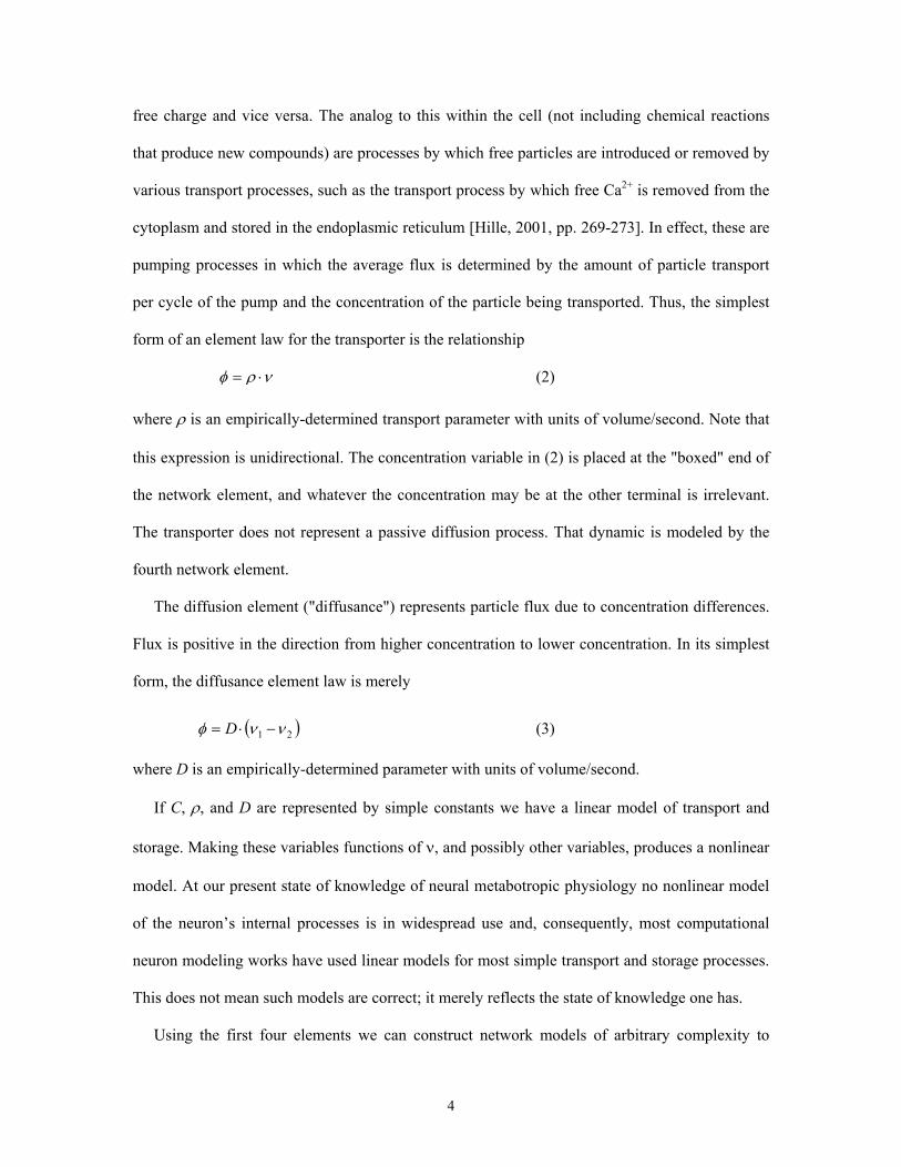
II. Simple Models of Ca2+ Processes in the Neuron The simplest and most common model of Ca2+ buffering in the neuron represents the gross

influx of Ca2+ from calcium channels and the removal of free Ca2+ from the cytoplasm by a

transport process. Figure 2 illustrates the model network. The endoplasmic reticulum is regarded

as having infinite volume and so the time rate of change of [Ca2+] at this node is zero. ICa is

obtained from the electrical model of the neuron, and its numerical value from the Goldman-

Hodgkin-Katz (GHK) current equation is negative or zero. Thus, the network of Figure 2 receives

an influx of Ca2+ into node ν. Summing the effluxes from this node, we obtain the dynamical

equation

( )tIdtdC Ca⋅−⋅−= βνρν . (4)

Figure 2: Simple model of free Ca2+ buffering. ICa is obtained from the electrical model of the neuron. Because its numerical value is negative, the Ca network receives a Ca2+ influx.

5

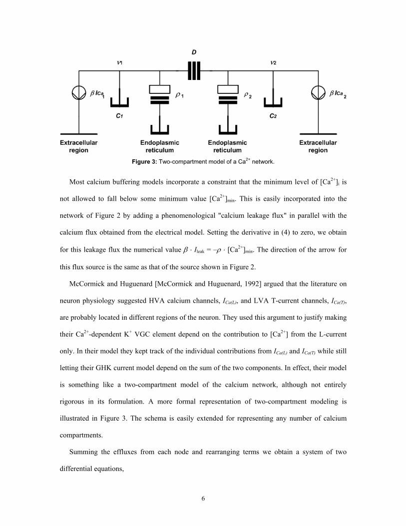
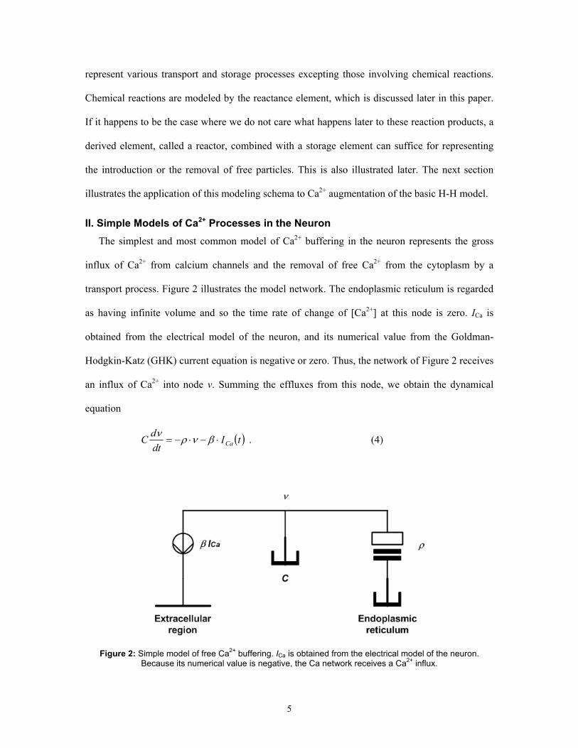
Figure 3: Two-compartment model of a Ca2+ network.

Most calcium buffering models incorporate a constraint that the minimum level of [Ca2+]i is

not allowed to fall below some minimum value [Ca2+]min. This is easily incorporated into the

network of Figure 2 by adding a phenomenological "calcium leakage flux" in parallel with the

calcium flux obtained from the electrical model. Setting the derivative in (4) to zero, we obtain

for this leakage flux the numerical value β ⋅ Ileak = –ρ ⋅ [Ca2+]min. The direction of the arrow for

this flux source is the same as that of the source shown in Figure 2.

McCormick and Huguenard [McCormick and Huguenard, 1992] argued that the literature on

neuron physiology suggested HVA calcium channels, ICa(L), and LVA T-current channels, ICa(T),

are probably located in different regions of the neuron. They used this argument to justify making

their Ca2+-dependent K+ VGC element depend on the contribution to [Ca2+] from the L-current

only. In their model they kept track of the individual contributions from ICa(L) and ICa(T) while still

letting their GHK current model depend on the sum of the two components. In effect, their model

is something like a two-compartment model of the calcium network, although not entirely

rigorous in its formulation. A more formal representation of two-compartment modeling is

illustrated in Figure 3. The schema is easily extended for representing any number of calcium

compartments.

Summing the effluxes from each node and rearranging terms we obtain a system of two

differential equations,

6

Figure 4: Simplified model of metabotropic-signal-induced calcium release.

( )

( )

−

−+

+−

+−=

2

1

22

11

2

1

222

111

2

1

00

Ca

Ca

II

CC

CDCDCDCD

dtddtd

ββ

νν

ρρ

νν

. (5)

As a final calcium example we will consider a metabotropic signaling process in which

internal Ca2+ stores are released from the endoplasmic reticulum to become free Ca2+ in the

cytoplasm. Figure 4 illustrates the model. This model is intended to illustrate the general ideas

conveyed by qualitative models of this process. It should be noted that our present state of

knowledge of the quantitative details of this process is incomplete and so the model presented

here is to be regarded as conceptual but not an established accurate representation of this process.

The model contains two types of chemical concentrations, [Ca2+]i represented on the left by

node variable Ca1, and cytoplasmic concentration of inositol triphosphate (IP3) represented by

node variable IP3 on the right. Ca2 represents the concentration of Ca2+ stored in the endoplasmic

reticulum (ER). Typical concentrations of stored Ca2+ is typically greater than 100 µM under

normal physiological conditions and likely reaches millimolar levels. The ER’s supply of Ca2+ is

by no means unlimited, but for normal signal processing functions we can regard the volume CER

as effectively infinite so that concentration Ca2 may be regarded as constant. We will also assume

flux source β⋅ICa1 includes a leakage flux that maintains the minimum level of Ca1 at its resting

concentration level (on the order of 50 to 100 nM). Transporter ρ1 is the same as described

7

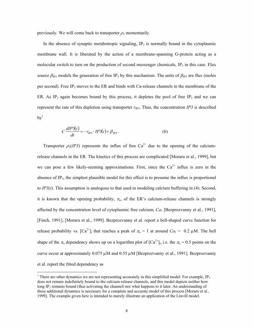
previously. We will come back to transporter ρ2 momentarily.

In the absence of synaptic metabotropic signaling, IP3 is normally bound in the cytoplasmic

membrane wall. It is liberated by the action of a membrane-spanning G-protein acting as a

molecular switch to turn on the production of second messenger chemicals, IP3 in this case. Flux

source βIP3 models the generation of free IP3 by this mechanism. The units of βIP3 are flux (moles

per second). Free IP3 moves to the ER and binds with Ca-release channels in the membrane of the

ER. As IP3 again becomes bound by this process, it depletes the pool of free IP3 and we can

represent the rate of this depletion using transporter rIP3. Thus, the concentration IP3 is described

by1

( ) ( ) IP3IP3 33 β+⋅−= tIPrdt

tdIPC . (6)

Transporter ρ2(IP3) represents the influx of free Ca2+ due to the opening of the calcium-

release channels in the ER. The kinetics of this process are complicated [Moraru et al., 1999], but

we can pose a few likely-seeming approximations. First, since the Ca2+ influx is zero in the

absence of IP3, the simplest plausible model for this effect is to presume the influx is proportional

to IP3(t). This assumption is analogous to that used in modeling calcium buffering in (4). Second,

it is known that the opening probability, πo, of the ER’s calcium-release channels is strongly

affected by the concentration level of cytoplasmic free calcium, Ca1 [Bezprozvanny et al., 1991],

[Finch, 1991], [Moraru et al., 1999]. Bezprozvanny et al. report a bell-shaped curve function for

release probability vs. [Ca2+]i that reaches a peak of πo = 1 at around Ca1 = 0.2 µM. The bell

shape of the πo dependency shows up on a logarithm plot of [Ca2+]i, i.e. the πo = 0.5 points on the

curve occur at approximately 0.075 µM and 0.55 µM [Bezprozvanny et al., 1991]. Bezprozvanny

et al. report the fitted dependency as

1 There are other dynamics we are not representing accurately in this simplified model. For example, IP3 does not remain indefinitely bound to the calcium-release channels, and this model depicts neither how long IP3 remains bound (thus activating the channel) nor what happens to it later. An understanding of these additional dynamics is necessary for a complete and accurate model of this process [Moraru et al., 1999]. The example given here is intended to merely illustrate an application of the Linvill model.

8

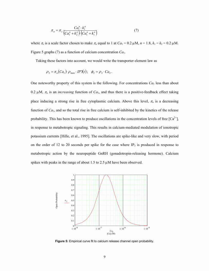
( ) ( )nnnn

nn

s kCakCakCa

1121

11o +⋅+

⋅= ππ (7)

where πs is a scale factor chosen to make πo equal to 1 at Ca1 = 0.2 µM, n = 1.8, k1 = k2 = 0.2 µM.

Figure 5 graphs (7) as a function of calcium concentration Ca1.

Taking these factors into account, we would write the transporter element law as

( ) ( ) 222max1o2 ;3 CatIPCa ⋅=⋅⋅= ρφρπρ .

One noteworthy property of this system is the following. For concentrations Ca1 less than about

0.2 µM, πo is an increasing function of Ca1, and thus there is a positive-feedback effect taking

place inducing a strong rise in free cytoplasmic calcium. Above this level, πo is a decreasing

function of Ca1, and so the total rise in free calcium is self-inhibited by the kinetics of the release

probability. This has been known to produce oscillations in the concentration levels of free [Ca2+]i

in response to metabotropic signaling. This results in calcium-mediated modulation of ionotropic

potassium currents [Hille, et al., 1995]. The oscillations are spike-like and very slow, with period

on the order of 12 to 20 seconds per spike for the case where IP3 is produced in response to

metabotropic action by the neuropeptide GnRH (gonadotropin-releasing hormone). Calcium

spikes with peaks in the range of about 1.5 to 2.5 µM have been observed.

1 .10 8 1 .10 7 1 .10 6 1 .10 50

0.1

0.2

0.3

0.4

0.5

0.6

0.7

0.8

0.9

1

[Ca] (M)

Ope

n Pr

obab

ility

π j

Caj

Figure 5: Empirical curve fit to calcium release channel open probability.

9

Summing effluxes from the Ca1 node and incorporating (6) gives us the system of first order

differential equations

⋅

−+

⋅

−

−=

3IP

221

IP3

111100

030

03

β

βρρCaI

Ca

CCC

IPCa

CrC

dtdIPdtdCa

. (8)

Although the equations in (8) appear to be uncoupled, in fact they are not. IP3 couples into the

first equation through ρ2.

An additional consideration not incorporated into this simplified model would account for loss

of free calcium through binding with the calcium-releasing channels depicted by ρ2. The kinetics

model of [Moraru et al., 1999] assumes two Ca2+ ions and four IP3 molecules participate in each

binding event at the receptor site for the calcium-releasing channels. This, however, could be

taken into account in an approximate fashion by the numerical value assigned to ρ2. More

important is the absence in the simplified model of a time-dependent rate process description for

transporters ρ2 and rIP3. In the simplest case we would have at least one additional differential

equation, possibly similar to a rate process model such as is used in the Hodgkin-Huxley schema,

capturing the opening- and closing-kinetics of the calcium releasing channels. Such a process

would affect the time-dependencies of both ρ2 and rIP3. Judging from the findings reported in

[Moraru et al., 1999], time constants for such a process are on the order of a few milliseconds.

As a final note, the model just presented is a very simplified representation of these dynamics.

Much more elegant treatments based on diffusion theory and partial differential equation models

have been formulated [Schutter and Smolen, 1998]. A lumped approximation for this type of model

would require the model of Figure 4 to be turned into a multi-compartment model.

III. The Reactance Element in the Linvill Modeling Schema

It is well known that metabotropic signaling plays an important control function in biological

signal processing. Metabotropic signaling occurs by means of cascade biochemical reactions in

10

the cell that alter basic properties in the flow of ionotropic signaling pathways. The reactance

element is the element in the Linvill network modeling schema that models chemical reactions.

The basic element shown in figure 1 has two inputs and one output. The reactance can be

easily extended to take into account more input reactants and/or to produce more than one

reaction product. In this section the action of the reactance element is illustrated for the simplest

case of two inputs and one output as shown in figure 6 below.

Consider the case of a simple chemical reaction in terms of concentrations of substances, e.g.,

321 22 ννν →+ .

We assume all three substances are co-located within the same volume within the cell. Because

the substances represent different chemical species, three storance elements are required, as

shown in the figure. Noting the flux directions indicated in the figure and applying the storance

element law, we have

332211 ;; νφνφνφ &&& CCC =−=−= .

Noting the stoichiometric coefficients in the chemical reaction equation above, we also have

1231 5.0; φφφφ ⋅== .

Chemical reaction kinetics are governed by the mole balance equation [Fogler, 1999, pp. 6-16]

and by the form of the reaction rate equation. In general, reaction rate equations are algebraic

equations, rather than differential equations, and are frequently deduced from experimental data.

Generally, a reaction rate equation would be of the form φi = fi(ν1,ν2,ν3) where fi is some algebraic

function of the concentrations of the three substances involved in the reaction [Fogler, 1999, pp.

73-113]. For purposes of our present example, we will assume the reaction is governed by the

simplest form of reaction rate expression, namely the second order reaction,

11

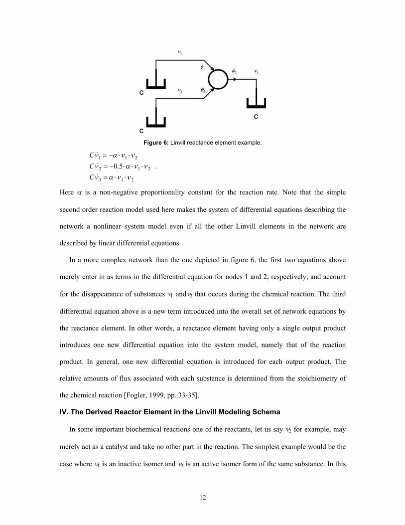
Figure 6: Linvill reactance element example.

C .

213

212

211

5.0νναν

νναννναν

⋅⋅=⋅⋅⋅−=

⋅⋅−=

&

&

&

C

C

Here α is a non-negative proportionality constant for the reaction rate. Note that the simple

second order reaction model used here makes the system of differential equations describing the

network a nonlinear system model even if all the other Linvill elements in the network are

described by linear differential equations.

In a more complex network than the one depicted in figure 6, the first two equations above

merely enter in as terms in the differential equation for nodes 1 and 2, respectively, and account

for the disappearance of substances ν1 andν2 that occurs during the chemical reaction. The third

differential equation above is a new term introduced into the overall set of network equations by

the reactance element. In other words, a reactance element having only a single output product

introduces one new differential equation into the system model, namely that of the reaction

product. In general, one new differential equation is introduced for each output product. The

relative amounts of flux associated with each substance is determined from the stoichiometry of

the chemical reaction [Fogler, 1999, pp. 33-35].

IV. The Derived Reactor Element in the Linvill Modeling Schema

In some important biochemical reactions one of the reactants, let us say ν2 for example, may

merely act as a catalyst and take no other part in the reaction. The simplest example would be the

case where ν1 is an inactive isomer and ν3 is an active isomer form of the same substance. In this

12

case we would have φ2 = 0 because catalyst ν2 is neither increased nor decreased by the reaction it

catalyzes. Often the reaction rate in such a case might involve a first-order reaction, f = α ⋅ν2, in

the expressions for φ1 and φ3. In such simple cases as this, the Linvill network can often be

simplified by the introduction of a sixth element, called a reactor, which is mathematically

identical to the transporter element in figure 1 except that the substances represented at the two

terminals are different substances. The reactor element can be regarded as a special case of a one-

input/one-output reactance.

At the present time, it is the unfortunate case that the research literature reporting the findings

of biochemical studies in neuroscience frequently omit findings regarding the specific reaction

rate kinetics of the biochemical reactions being studied. It can be hoped that the introduction of

the Linvill modeling schema may help to change this situation. In the absence of reported

experimental facts, the mathematical modeler can only have recourse to phenomenological

guesses of what form of reaction rate equation f might be involved in a particular system under

study. Quantitative results from such modeling work can serve to pose questions to other

researchers that subsequent experiments can confirm or refute. One example of this is a recent

work by Ramirez on modeling of monoclonal antibodies in the treatment of methamphetamine

addiction [Ramirez, 2008].

It has been well established that phosphorylation/dephosphorylation is an important, and

perhaps the primary, mechanism for regulating receptor sensitivity and modulating ion channel

dynamics [Huganir and Greengard, 1990], [Levitan, 1994]. While physiologists, molecular biologists,

and neurochemists have long been aware of the importance of phosphorylation/dephosphorylation

in the regulation of neuronal activity, this has not yet been widely recognized by neural network

theorists in the form of neural network models that include it in their structures. Of the major

schools of neural network theory, only adaptive resonance theory has so far incorporated

mathematics to give a well-organized account for the modulation phenomena, albeit this

13

accounting is high-level, abstract, and quite indirect. Yet most of the major subsystems in the

brain that signal by means of metabotropic messengers have widespread targets across large

regions of the neocortex and other cerebral structures. Because these modulating signals work

through phosphorylation and dephosphorylation, this lack of attention by neural network theorists

is difficult to justify.

Not surprisingly, the kinetics of phosphorylation are different for the many different kinds of

kinases. We will not delve into the fine details of the biochemistry involved here, mainly because

there are so many but also because this is a topic for specialists. Some excellent reviews are

available describing PKA [Francis and Corbin, 1994], PKC [Tanaka and Nishizuka, 1994], the

CaM kinases [Hanson and Schulman, 1992], and the receptor tyrosine kinases [Fantl et al., 1993].

In this paper the focus will be given to common features found in the processes of the

phosphorylation/dephosphorylation cycle.

A kinase exhibits (at least) two states, called active and inactive. A kinase in the active state

produces phosphorylation of its target substrate protein. Phosphorylation is often ATP-dependent,

and it produces compounds which are highly reactive in water with other organic molecules in the

presence of appropriate enzymes. An inactive kinase is one in a configuration where it does not

act as such a catalyst.

Second messengers cause a kinase to enter the active state. Other factors in the cell’s chemical

milieu, not all of which are particularly well understood, return a kinase to its inactive (basal)

state. In addition to phosphorylating substrate proteins, some kinases have the ability to

phosphorylate themselves; this is called autophosphorylation. A kinase in this state remains at

least partially active and is returned to the inactive state through the action of a phosphatase. Let

S0 denote the inactive state of a kinase. Let S1 represent the normal active state of the kinase, and

let S2 represent the autophosphorylated active state.

By introducing a new element in the Linvill modeling schema, called the reactor, we can

represent the process just described. The simplest feasible representation is shown in Figure 7.

14

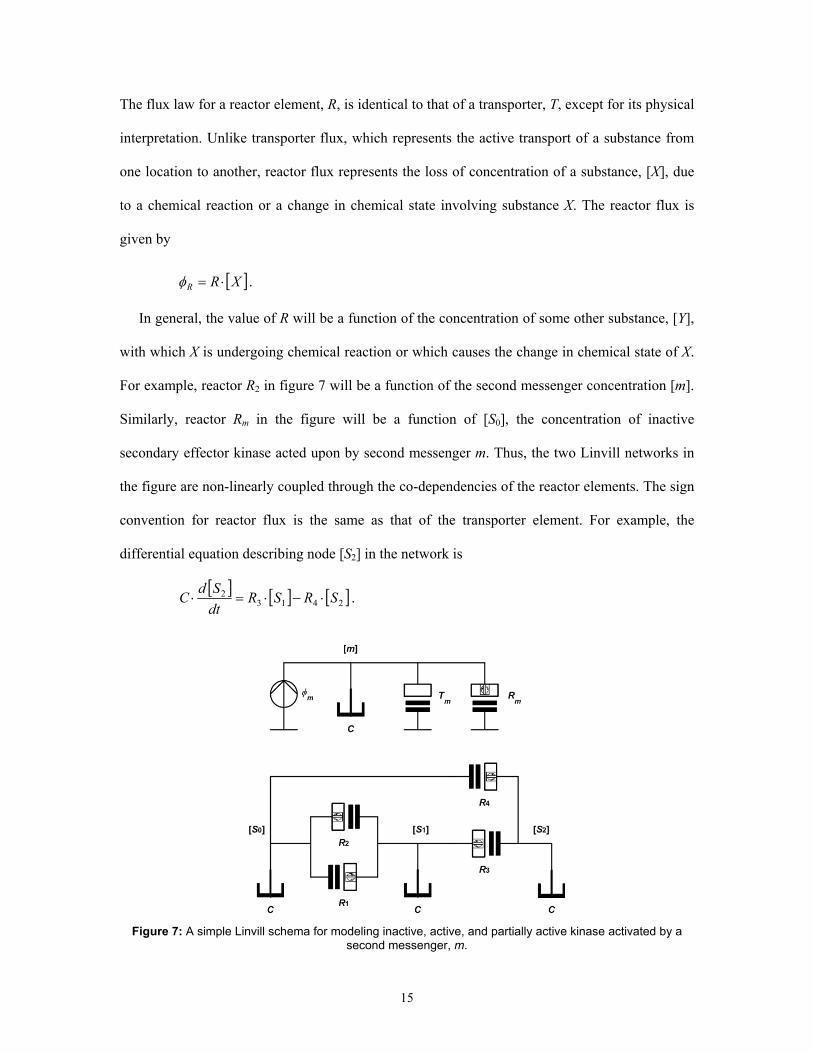
The flux law for a reactor element, R, is identical to that of a transporter, T, except for its physical

interpretation. Unlike transporter flux, which represents the active transport of a substance from

one location to another, reactor flux represents the loss of concentration of a substance, [X], due

to a chemical reaction or a change in chemical state involving substance X. The reactor flux is

given by

[ ]XRR ⋅=φ .

In general, the value of R will be a function of the concentration of some other substance, [Y],

with which X is undergoing chemical reaction or which causes the change in chemical state of X.

For example, reactor R2 in figure 7 will be a function of the second messenger concentration [m].

Similarly, reactor Rm in the figure will be a function of [S0], the concentration of inactive

secondary effector kinase acted upon by second messenger m. Thus, the two Linvill networks in

the figure are non-linearly coupled through the co-dependencies of the reactor elements. The sign

convention for reactor flux is the same as that of the transporter element. For example, the

differential equation describing node [S2] in the network is

[ ] [ ] [ ]24132 SRSR

dtSd

⋅−⋅=⋅C .

Figure 7: A simple Linvill schema for modeling inactive, active, and partially active kinase activated by a

second messenger, m.

15

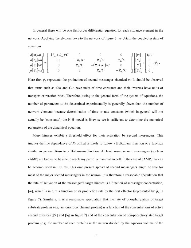
In general there will be one first-order differential equation for each storance element in the

network. Applying the element laws to the network of figure 7 we obtain the coupled system of

equations

[ ][ ][ ][ ]

( )

( )

[ ][ ][ ][ ]

m

mm C

SSSm

CRCRCRRCR

CRCRCRCRT

dtSddtSddtSd

dtmd

φ⋅

+

⋅

−+−

−+−

=

000

1

0000

0000

2

1

0

43

312

412

2

1

0 .

Here flux φm represents the production of second messenger chemical m. It should be observed

that terms such as C/R and C/T have units of time constants and their inverses have units of

transport or reaction rates. Therefore, owing to the general form of the system of equations, the

number of parameters to be determined experimentally is generally fewer than the number of

network elements because determination of time or rate constants (which in general will not

actually be "constants"; the H-H model is likewise so) is sufficient to determine the numerical

parameters of the dynamical equation.

Many kinases exhibit a threshold effect for their activation by second messengers. This

implies that the dependency of R2 on [m] is likely to follow a Boltzmann function or a function

similar in general form to a Boltzmann function. At least some second messengers (such as

cAMP) are known to be able to reach any part of a mammalian cell. In the case of cAMP, this can

be accomplished in 100 ms. This omnipresent spread of second messengers might be true for

most of the major second messengers in the neuron. It is therefore a reasonable speculation that

the rate of activation of the messenger’s target kinases is a function of messenger concentration,

[m], which is in turn a function of its production rate by the first effector (represented by φm in

figure 7). Similarly, it is a reasonable speculation that the rate of phosphorylation of target

substrate proteins (e.g. an ionotropic channel protein) is a function of the concentrations of active

second effectors ([S1] and [S2] in figure 7) and of the concentration of non-phosphorylated target

proteins (e.g. the number of such proteins in the neuron divided by the aqueous volume of the

16

cell). Modeling this requires that a third subnetwork, along the same lines as the lower

subnetwork in figure 7, be added to the total network model.

V. Discussion

The principal protein kinases are widely expressed throughout the central nervous system.

Often they are heavily concentrated in the postsynaptic density. Because these membrane

spanning proteins are target substrate proteins for active kinases, this localization is further

evidence for how the modulatory role of these kinases is realized in biological signal processing.

At the present state of signal processing model theory for the neuron, there are many

important factors for which we are not yet in possession of quantitative data needed to develop an

accurate model. No doubt a large of amount of this information lies buried in the biochemistry

and organic chemistry literature, e.g. [Buxbaum and Dudai, 1989], expressed there in the

language of the chemist rather than that of the neuroscientist. No doubt, too, some of this

information is still entirely unknown, the relevant modeling research question not having yet been

posed. This is an under-recognized research field for computational neuroscience and biological

signal processing. There is very clear evidence that for many of the important kinases their

activity level (which one can assess by examining the rates at which they phosphorylate their

targets) is more complex than being merely binary or ternary (as figure 7 might suggest). Reports

in the bio-chemistry literature indicate that the activity levels of the major kinases is dependent

upon levels of ATP concentration and probably other factors as well. Accounting for this clearly

requires a more complex network model than the example given above. Indeed, the need for this

accounting is one reason why a method of lumped-element representation of the process is useful

and important for understanding the modulation processes of the neuron.

The experimentally observed fact that many of the major protein kinases, especially PKC and

CaM, exhibit autophosphorylation, and thus remain partially active even after concentration

levels of their second messengers decline, has been a source of great scientific interest. There is a

good deal of speculation that autophosphorylation of the kinases is a memory mechanism for the

17

neuron [Schwartz and Greenberg, 1987]. This appears to be an undeniable fact in the case of

elastic modulation, a form of short-term memory for the neuron. Additional evidence suggests

that some kinases, particularly CaM and presynaptic PKC, may also support plastic (that is,

irreversible) modulation of synaptic efficacy. Presently, this putative role is still somewhat

speculative, but it is receiving a great deal of attention and one can reasonably expect the future to

bring further clarification to this possibility. It is clear that, as a flexible modeling schema, the

Linvill modeling schema has the potential to play an important quantitative role in this research.

The secondary effectors primarily exert their effects through phosphorylation of their target

substrate proteins. The phosphorylation process is accompanied by another regulatory process,

namely the process of dephosphorylation. Phosphorylation of the substrate protein can, depending

on the kinase involved and the particulars of the target protein, work either to sensitive or to

desensitize the response of the channel protein in responding to neurotransmitters. In some cases

it can open a normally-closed channel; in others it can close a normally-open channel. One model

of this effect, although disputed by some researchers, holds that phosphorylation of channel

proteins can be represented by introducing the idea of an effective density of channel proteins in

the synapse. In this phenomenological model, the effect of phosphorylation is looked upon as

having the same effect as increasing (or decreasing) the number of receptors on the postsynaptic

side of the synapse. AMPA receptors are often treated this way, although there seems to be no

strong reason to exclude the other ionotropic receptors from being looked at in this way.

However, as already noted, other researchers take issue with this model of cell response to the

secondary effectors, and the matter seems to be far from settled on the physiology level.

Computational neuroscientists, on the other hand, have been quick to adopt this model of channel

sensitization/desensitization. Better quantitative modeling can be expected to help bring the issue

to a better determination.

Presynaptic protein kinases might possibly target synaptic vesicle membranes or other

structures within the synaptic terminal and thereby effect a change in the efficacy of

18

neurotransmitter exocytosis. This is presently regarded as rather speculative and is often

accompanied by the hypothesis that membrane-permeable retrograde messengers such as NO

must also be involved in such a process. NO is a byproduct of the action of the arachidonic acid

(AA) process; the DAG-PKC second messenger process is thought to produce AA as a

divergence byproduct. Putative mechanisms such as these are easily added to theoretical models

by means of the appropriate Linvill network.

Dephosphorylation is the removal of the phosphate group from the target protein. It is also the

mechanism by which autophosphorylated protein kinases become inactive once again.

Dephosphorylation is produced by enzymes called phosphoprotein phosphatases. Whatever the

cell response to the secondary effector was, dephosphorylation terminates the effect. Reactor R4

in figure 7, which represents dephosphorylation of an autophosphorylated kinase, is an example

of how the Linvill modeling schema can represent of this effect. A large value of R4 (or,

equivalently, R4/C) represents rapid dephosphorylation; a small value represents slow

dephosphorylation.

Dephosphorylation can itself be regulated by metabotropic mechanisms. One well-studied

case is that of phosphorylation of K+ channels by the action of PKA [Siegelbaum et al., 2000]. In

this case, a K+ channel opened by phosphorylation is dephosphorylated and closed by the action

of phosphoprotein phosphatase-1. However, the action of this enzyme is regulated by another

protein, inhibitor-1. Inhibitor-1 is phosphorylated by the action of PKA, and in this state it

inhibits the action of phosphoprotein phosphatase-1. Here is one example of how one

metabotropic signaling cascade can diverge (PKA inhibiting dephosphorylation, while at the

same time producing it in the K+ channel). Inhibitor-1 is dephosphorylated by the action of Ca2+,

which activates the phosphatase calcineurin that in turn dephosphorylates inhibitor-1. A similar

process has been reported for regulating phosphorylation/dephosphorylation of NMDA receptors

[Halpain et al., 1990]. This one involves inactivation of the inhibitor DARPP-32 by CaM and

activation of DARPP-32 by PKA produced from elevated cAMP levels stimulated by dopamine

19

signaling.

Each of these actions just described can be approximated by adding additional Linvill

networks to those depicted in figure 7. In the case of targeted channel proteins, if one adopts the

effective-density model the relevant concentrations would be concentrations νp of phosphorylated

channels and νd of dephosphorylated channels. Reactor elements would be used to model the

kinetics of the phosphorylation/dephosphorylation process in terms of concentrations of various

active secondary effectors. Modeling of dephosphorylation would involve networks, similar to

the lower network in figure 7, modeling the concentrations of inhibited and uninhibited

phosphatases, calcineurin, etc.

Perhaps the principal significance of all of this is the following. The Linvill modeling schema

provides a more or less straightforward way for the investigator to proceed from a qualitative

model of putative mechanisms, such as are common in neurobiology, to quantitative

mathematical models of the hypothesis. This process not only brings into prominence the key

factors required to obtain specific predictions and implications of a theory, but also points toward

new experiments addressed to the purpose of discovering quantitative information about these

mechanisms. In this way, models assist in the logical progression of research programs and are a

source of significant research questions and aims. Furthermore, one need not be a highly trained

mathematician in order to be able to propose such mathematical models. Ramirez, for example,

had no more than a basic knowledge of calculus and yet was able to produce a interesting and

fairly accurate model of monoclonal antibody kinetics from a starting point of merely qualitative

information regarding the putative action of these antibodies in treating methamphetamine

addiction [Ramirez, 2008].

In conclusion, this paper has presented the Linvill modeling schema as an efficient approach

for the development of quantitative models and theories in biochemical cascade reaction signaling

(metabotropic signaling). It is proposed that this methodology holds much research promise.

20

References

Bezprozvanny, I., J. Watras and B.E. Ehrlich, "Bell-shaped calcium-response curves of Ins(1,4,5)P3- and calcium-gated channels from endoplasmic reticulum of cerebellum," Nature (Lond.), 351: 751-754, 1991.

Buxbaum, Daniel J. and Yadin Dudai, "A quantitative model for the kinetics of cAMP-dependent protein kinase (type II) activity," J. Biol. Chem., vol. 264, no. 16, June 5, 1989, pp. 9344-9351.

Fantl, Wendy J., Daniel E. Johnson, and Lewis T. Williams, "Signalling by receptor tyrosine kinases," Annu. Rev. Biochem., 62: 453-481, 1993.

E.A. Finch, E.A., T.J. Turner and S.M. Goldin, "Calcium as a coagonist of inositol 1,4,5-triphosphate-induced calcium release," Science, 252: 443-446, 1991.

Fogler, H. Scott, Elements of Chemical Reaction Engineering, 3rd ed., Upper Saddle River, NJ: Prentice-Hall, 1999.

Francis, Sharron H. and Jackie D. Corbin, "Structure and function of cyclic nucleotide-dependent protein kinases," Annu. Rev. Physiol., 56: 237-272, 1994.

Halpain, Shelley, Jean-Antoine Girault, and Paul Greengard, "Activation of NMDA receptors induces dephosphorylation of DARPP-32 in rat striatal slices," Nature, vol. 343, pp. 369-372, Jan., 1990.

Hanson, Phyllis I. and Howard Schulman, "Neuronal Ca2+/calmodulin-dependent protein kinases," Annu. Rev. Biochem., 61: 559-601, 1992.

Hille, B., A. Tse, F.W. Tse and M.M. Bosma, "Signaling mechanisms during the response of pituitary gonadotropes to GnRH," Recent Prog. Horm. Res., 50: 75-95, 1995.

Hille, Bertil, Ion Channels of Excitable Membranes, 3rd ed. Sunderland, MA: Sinauer Associates, 2001.

Huganir, Richard L. and Paul Greengard, "Regulation of neurotransmitter receptor desensitization by protein phosphorylation," Neuron, 5: 555-567, Nov., 1990.

Levitan, Irwin B., "Modulation of ion channels by protein phosphorylation and dephosphorylation," Annu. Rev. Physiol., 56: 193-212, 1994.

J.G. Linvill, J.G. and J.F. Gibbons, Transistors and Active Circuits, NY: McGraw-Hill, 1961.

McCormick, D.A. and J.R. Huguenard, "A model of the electrophysiological properties of thala-mocortical relay neurons," J. Neurophysiol., 68: 1384-1400, 1992.

Moraru, I.I., E.J. Kaftan, B.E. Ehrlich and J. Watras, "Regulation of type 1 inositol 1,4,5-triphosphaste-gated calcium channels by InsP3 and calcium: Simulation of single channel kinetics based on ligand binding and electrophysiological analysis," J. Gen. Physiol., 113: 837-849, 1999.

Ramirez, Sarahi, "Modeling the effect of monoclonal antibodies in the treatment of methamphetamine addiction using the Linvill modeling schema," poster presentation, Sigma Xi Annual Meeting and Student Research Competition, Washington, DC, Nov. 21, 2008.

Schutter, Erik De and Paul Smolen, "Calcium dynamics in large neuronal models," in Methods in Neuronal Modeling, 2nd ed., C. Koch and I. Segev (Eds.), Cambridge, MA: The MIT Press, 1998, pp. 211-250.

Schwartz, James H. and Steven M. Greenberg, "Molecular mechanisms for memory: Second-messenger induced modifications of protein kinases in nerve cells," Annu. Rev. Neurosci., 10: 459-476, 1987.

Siegelbaum, Steven A., James H. Schwartz, and Eric R. Kandel, "Modulation of synaptic transmission: Second messengers", in Principles of Neural Science, 4th ed. (Eric R. Kandel, James H. Schwartz, and Thomas M. Jessell, Eds.), NY: McGraw-Hill, 2000, pp. 229-252

Tanaka, Chikako and Yasutomi Nishizuka, "The protein kinase C family for neuronal signaling," Annu. Rev. Neurosci., 17: 551-567, 1994.

21