Embed Size (px)
Citation preview

POLITECNICO DI TORINO
Master degree course in Mechatronic Engineering
Master Degree Thesis
A Machine Learning Technique forPredictive Maintenance and Quality
in Cut Glass Machinery
Supervisors
prof. Edoardo PattiAndrea AcquavivaLorenzo BottaccioliLuciano Baresi
Candidate
Giacomo Ornati
2019 October


Abstract
The study presented in this thesis work is based on the development ofa machine learning project applied to the particular case of the 548 Lammachine, a cut glass machine produced by the company Bottero s.p.a.,which collaborates with this thesis. The work describes how to developa project based on machine learning and how it can be applied in a realcase. The thesis is in fact divided into two distinct parts, the first moredidactic in which are explained the various steps to be followed to preparethe data and apply different algorithms of machine learning to maximizethe results, the second instead shows how to use in a concrete way theresults of the study of machine learning in order to effectively increaseproductivity. To do this, two problems have been selected to be solved,indicated by the company.
The first study tries to predict machine stops and anomalous failures.The work includes an accurate understanding of the machine and thestarting dataset, and then concentrate on the data preparation. There-fore, all the various steps to be followed during the pre-processing phaseare listed: how to perform data merging, correlational and statisticalanalysis to find important information from the data, feature selection,how to manage categorical features. When the initial data have beenproperly manipulated, we proceed to the evaluation phase of the selectedalgorithms based on the characteristics of the dataset, evaluating whichmodel obtains the best results in predicting machine errors. The resultsobtained show that the probabilistic algorithms based on the tree classi-fication are those that best predict errors. In details, the Random ForestClassifier proves to be the best model obtaining an F1 score of about 50%on the positive prediction.
The second part deals with the prediction of machining times basedon the characteristics of the work to be performed. This second part wantto show how a machine learning model can be transposed from the merefield of study to a real application, so there is a reconstruction of theprediction function inside the machine itself, in order to make real timepredictions based on the data selected by the user. The linear regressionmodel was first trained on a PC thanks to the data contained in thedataset and then reconstructed in the software interface of the machinethanks to the coefficients listed in an orderly JSON file that is first createdduring the training of the model and then passed to the machine that isat this point able to make predictions. The results show that the timeprediction based on this model achieves an error of less than 10% withrespect to the actual measured values.
iii


Contents
List of Figures viii
List of Tables x
1 Introduction 11.1 Scope of this work and problem formulation . . . . . . . . 11.2 Error Prediction . . . . . . . . . . . . . . . . . . . . . . . . 21.3 Time Prevision . . . . . . . . . . . . . . . . . . . . . . . . 31.4 How the work was structured . . . . . . . . . . . . . . . . 4
2 The machinary and the process 72.1 Functional groups . . . . . . . . . . . . . . . . . . . . . . . 82.2 Phases of interest and criticalities . . . . . . . . . . . . . . 102.3 The process of cutting the laminated glass . . . . . . . . . 12
2.3.1 Trim cuts . . . . . . . . . . . . . . . . . . . . . . . 152.4 The machine control software . . . . . . . . . . . . . . . . 16
2.4.1 Interface management . . . . . . . . . . . . . . . . 17
3 Database and Data Collection 213.1 Structure of the database . . . . . . . . . . . . . . . . . . . 21
3.1.1 Session event . . . . . . . . . . . . . . . . . . . . . 233.1.2 MachineState event . . . . . . . . . . . . . . . . . . 233.1.3 Step event . . . . . . . . . . . . . . . . . . . . . . . 243.1.4 Cut event . . . . . . . . . . . . . . . . . . . . . . . 253.1.5 Glass event . . . . . . . . . . . . . . . . . . . . . . 253.1.6 Piece event . . . . . . . . . . . . . . . . . . . . . . 263.1.7 TypeOfGlassBasicParameters event . . . . . . . . . 263.1.8 MachineError event . . . . . . . . . . . . . . . . . . 263.1.9 Other events . . . . . . . . . . . . . . . . . . . . . . 28
3.2 How and when the data is sent . . . . . . . . . . . . . . . 283.3 Raw Data Manipulation on the Database for Time Prevision 29
v

4 Machine Learning: Main Supervised Characteristics andAlgorithms 314.1 Supervised Learning . . . . . . . . . . . . . . . . . . . . . 32
4.1.1 General Structure . . . . . . . . . . . . . . . . . . . 334.1.2 Classification and Regression . . . . . . . . . . . . . 364.1.3 Underfitting and Overfitting . . . . . . . . . . . . . 364.1.4 Bias and Variance . . . . . . . . . . . . . . . . . . . 384.1.5 Evaluation Metrics . . . . . . . . . . . . . . . . . . 43
4.2 Classification Learning Algorithms . . . . . . . . . . . . . 464.2.1 Logistic Regression . . . . . . . . . . . . . . . . . . 464.2.2 Naive Bayas . . . . . . . . . . . . . . . . . . . . . . 484.2.3 Support Vector Machine . . . . . . . . . . . . . . . 494.2.4 Random Forest Classifier . . . . . . . . . . . . . . . 514.2.5 Nearest Neighbor . . . . . . . . . . . . . . . . . . . 524.2.6 Neural Networks . . . . . . . . . . . . . . . . . . . 544.2.7 Linear Discriminant Analysis and Principal Com-
ponent Analysis . . . . . . . . . . . . . . . . . . . . 564.3 Regression Learning Algorithms . . . . . . . . . . . . . . . 57
4.3.1 Linear Regression . . . . . . . . . . . . . . . . . . . 584.3.2 Polynomial Regression . . . . . . . . . . . . . . . . 594.3.3 Ridge and Lasso Regression . . . . . . . . . . . . . 604.3.4 Support Vector Regression . . . . . . . . . . . . . . 61
4.4 Supervised Algorithm Choice . . . . . . . . . . . . . . . . 624.4.1 Choose feasible algorithms . . . . . . . . . . . . . . 624.4.2 Best algorithm selection . . . . . . . . . . . . . . . 65
5 Error Prediction: Data Preparation 675.1 A bug in manual mode data collection . . . . . . . . . . . 685.2 Data merging . . . . . . . . . . . . . . . . . . . . . . . . . 69
5.2.1 Basic idea . . . . . . . . . . . . . . . . . . . . . . . 715.2.2 Cut table . . . . . . . . . . . . . . . . . . . . . . . 725.2.3 Associate Step event . . . . . . . . . . . . . . . . . 725.2.4 Associate other events, the example of Session event 745.2.5 Final reshape . . . . . . . . . . . . . . . . . . . . . 77
5.3 Handle Categorical Features . . . . . . . . . . . . . . . . . 775.3.1 Common methods . . . . . . . . . . . . . . . . . . . 795.3.2 Application on the case study . . . . . . . . . . . . 81
5.4 Correlation analysis . . . . . . . . . . . . . . . . . . . . . . 825.4.1 In theory . . . . . . . . . . . . . . . . . . . . . . . 835.4.2 In practice . . . . . . . . . . . . . . . . . . . . . . . 85
5.5 Statistical analysis . . . . . . . . . . . . . . . . . . . . . . 905.5.1 Unbalanced dataset . . . . . . . . . . . . . . . . . . 90
vi

5.5.2 Differences among customers . . . . . . . . . . . . . 925.6 Feature selection . . . . . . . . . . . . . . . . . . . . . . . 95
5.6.1 Manual features selection . . . . . . . . . . . . . . . 965.6.2 Automatic features selection . . . . . . . . . . . . . 975.6.3 Some algorithms implementation in the real dataset 99
6 Error Prediction: Algorithm evaluation 1036.1 Training and Test sets and Normalization . . . . . . . . . . 1036.2 Evaluation Metric Choice . . . . . . . . . . . . . . . . . . . 1056.3 Hyperparameters tuning . . . . . . . . . . . . . . . . . . . 106
6.3.1 Grid Search . . . . . . . . . . . . . . . . . . . . . . 1076.4 Results for each client . . . . . . . . . . . . . . . . . . . . 1076.5 Notes on performances . . . . . . . . . . . . . . . . . . . . 1126.6 Algorithm Choice . . . . . . . . . . . . . . . . . . . . . . . 113
6.6.1 Random forest learning curve . . . . . . . . . . . . 113
7 Time Prevision Solution 1177.1 Requirement . . . . . . . . . . . . . . . . . . . . . . . . . . 1177.2 Starting Data . . . . . . . . . . . . . . . . . . . . . . . . . 1187.3 Idea . . . . . . . . . . . . . . . . . . . . . . . . . . . . . . 1197.4 Implementation . . . . . . . . . . . . . . . . . . . . . . . . 120
7.4.1 548 Lam implementation . . . . . . . . . . . . . . . 1227.4.2 Validation of the performance . . . . . . . . . . . . 123
7.5 Results . . . . . . . . . . . . . . . . . . . . . . . . . . . . . 1247.6 Further Applications . . . . . . . . . . . . . . . . . . . . . 125
8 Final Observations and Comments 129
9 Appendix 1 1339.1 Programming Environment . . . . . . . . . . . . . . . . . . 133
9.1.1 Jupyter Notebook . . . . . . . . . . . . . . . . . . . 1339.1.2 Python . . . . . . . . . . . . . . . . . . . . . . . . . 1349.1.3 Pandas . . . . . . . . . . . . . . . . . . . . . . . . . 1349.1.4 SKLearn, NumPy, SciPy . . . . . . . . . . . . . . . 1349.1.5 Other libraries . . . . . . . . . . . . . . . . . . . . . 135
9.2 Structure of the work . . . . . . . . . . . . . . . . . . . . . 1389.2.1 Error Prediction: Scripts Structure and Division . . 1389.2.2 Time Prevision Script . . . . . . . . . . . . . . . . 138
Bibliography 147
vii

List of Figures
2.1 Basic setup of a 548 Lam machine . . . . . . . . . . . . . . . 82.2 TTS module of a 548 Lam machine . . . . . . . . . . . . . . 92.3 The loading table of a 548 Lam machine . . . . . . . . . . . . 102.4 Workbench of a 548 Lam machine . . . . . . . . . . . . . . . 102.5 Laminated glass general structure . . . . . . . . . . . . . . 132.6 Steps for cutting laminated glass . . . . . . . . . . . . . . 152.7 Process of trim cut . . . . . . . . . . . . . . . . . . . . . . 162.8 Editor menu . . . . . . . . . . . . . . . . . . . . . . . . . . 172.9 Automatic menu . . . . . . . . . . . . . . . . . . . . . . . 182.10 Type of glass selection and tuning . . . . . . . . . . . . . . 192.11 Manual mode . . . . . . . . . . . . . . . . . . . . . . . . . 20
4.1 Different fit of the data set . . . . . . . . . . . . . . . . . . 354.2 A simple representation of a cost function . . . . . . . . . 354.3 Overfitting and underfitting for a simple classification prob-
lem . . . . . . . . . . . . . . . . . . . . . . . . . . . . . . . 374.4 Correlation errors/fitting in function of model complexity . 384.5 Learning curve that seems to perform well . . . . . . . . . 404.6 Learning curve for high variance dataset . . . . . . . . . . 414.7 Learning curve for high bias . . . . . . . . . . . . . . . . . 424.8 Sigmoid function: hypothesis function for logistic regression 474.9 SVM: large margin classifier . . . . . . . . . . . . . . . . . 504.10 RFC: general structure of a Random Forest Classifier . . . 524.11 KNN: classification changes basis on different k . . . . . . 534.12 Neural Network: a typical structure . . . . . . . . . . . . . 554.13 PCA and LDA representation in a two features size database 574.14 A typical example of linear regression fitting in 2D. . . . . . . 594.15 Polynomial regression, the hypothesis function is now a curve. . 604.16 Support vector regression with the usage of tolerance range for
finding the maximum margin. . . . . . . . . . . . . . . . . . 62
5.1 Bad terminated cuts occurrency in function of cut length . 68
viii

5.2 Automatic and manual occurrency of bad terminated cuts 695.3 The discovered bug affects all the clients . . . . . . . . . . 705.4 Process of cut table creation . . . . . . . . . . . . . . . . . 735.5 Step table creation flow chart . . . . . . . . . . . . . . . . 745.6 Merging of cut and step table by inner join . . . . . . . . . 755.7 Creation of Cut+Step+Session table . . . . . . . . . . . . 765.8 Three example of scatter plots and relative Pearson coeffi-
cient . . . . . . . . . . . . . . . . . . . . . . . . . . . . . . 845.9 Pearson correlation coefficients matrix . . . . . . . . . . . 865.10 Kendall correlation coefficients matrix . . . . . . . . . . . . 875.11 Spearman correlation coefficients matrix . . . . . . . . . . 885.12 Correlation matrix for the firt client . . . . . . . . . . . . 895.13 Correlation matrix for the second client . . . . . . . . . . 905.14 Correlation matrix for the third client . . . . . . . . . . . 915.15 Cut length divided by clients . . . . . . . . . . . . . . . . . 925.16 Thickness of cut glass divided by clients . . . . . . . . . . 945.17 Pression used for upper truncation divided by clients . . . 945.18 Normalized standard deviation reduction plot . . . . . . . 1015.19 Code for implement the univariate statistical test features
selection . . . . . . . . . . . . . . . . . . . . . . . . . . . . 102
6.1 Process of training and testing with cross-validation . . . . . . 1056.2 Client 1 in manual feature selection . . . . . . . . . . . . . 1086.3 Client 1: automatic feature selection . . . . . . . . . . . . 1096.4 Client 2: manual feature selection scores . . . . . . . . . . 1106.5 Client 2: automatic feature selection results . . . . . . . . 1106.6 Client 3: manual feature selection scores . . . . . . . . . . 1116.7 Client 3: automatic feature selection algorithms evaluation 1116.8 Random forest learning curve for client 1 . . . . . . . . . . 1146.9 Learning curve for client 2 . . . . . . . . . . . . . . . . . . . 1146.10 Learning curve for client 3 . . . . . . . . . . . . . . . . . . . 115
7.1 Data preparation phase for time prevision. . . . . . . . . . . . 1197.2 Data flow of time prevision . . . . . . . . . . . . . . . . . . 1217.3 JSON file example . . . . . . . . . . . . . . . . . . . . . . 1237.4 Implementation of time prevision inside 548 Lam . . . . . 1237.5 Validation process . . . . . . . . . . . . . . . . . . . . . . . 1247.6 Client A time prediction results from validation process . . 1267.7 Client B results from validation process . . . . . . . . . . . 127
9.1 A typical interface of Jupyter Notebook . . . . . . . . . . . . 134
ix

List of Tables
3.1 Format of TEvent table . . . . . . . . . . . . . . . . . . . 223.2 List of all possible errors for 548 Lam . . . . . . . . . . . . 27
4.1 Reducing Bias and Variance . . . . . . . . . . . . . . . . . 394.2 Confusion matrix for binary classification . . . . . . . . . . 44
5.1 Schematic shape of table obtained after data merging . . . 725.2 Features after data merging . . . . . . . . . . . . . . . . . 785.3 Features after handling categorical features . . . . . . . . . 825.4 Historic review of the output to predict divided by client . 915.5 Mean and Standard Deviation divided by clients for au-
tomaic cuts . . . . . . . . . . . . . . . . . . . . . . . . . . 93
6.1 Hyperparameters tuned after grid search . . . . . . . . . . 107
x


Chapter 1
Introduction
1.1 Scope of this work and problem formula-tion
This thesis work was born from the will of the company Bottero s.p.a.to expand its knowledge in the Internet of Thinks (IoT) and ArtificialIntelligence (AI) field. Specifically it acts on data collected by one oftheir machines: the 548 Lam for cutting laminated glass. The purpose ofthis thesis is to try, thanks to the analysis of the data collected by thesemachines, to predict its possible behavior in a perspective of predictivemaintenance and predictive quality.
More in detail, the work that will be presented consists of two mainparts: Error Prediction and Time Prevision. Both are works relatedto the world of Machine Learning (ML) that use as a starting point theBottero database full of information from machines already produced andin operation in the possession of various customers around the world.
The initial purpose of the database was to collect information for sta-tistical purposes of the company. Bottero then realized the potential ofthe collected data that can be used for more complex and productivepurposes such as increasing the quality of the machine, avoiding errorsor adding functionality in a simple way thanks to the fact that the IoTecosystem was already complete from the point of view of data collection,to complete it was missing only a prudent use of the database to achieveimprovements and optimizations. This prudent use is a correct applica-tion of artificial intelligence that allows to obtain substantial achievementsonly thanks to data analysis.
This work therefore represents common parts for both Error Predic-tion and Time Prevision that are: a study of the machinery, of the working
1

1 – Introduction
process and of the database containing the information related to the lat-ter in such a way as to be able to find the machine learning algorithms thatbest behave with the object of study in question. Then a detailed studyfor each of the two sections will be performed: it will analyze the maincharacteristics of various algorithms known in the literature, highlightingtheir pros and cons. Finally, the results obtained by implementing thesealgorithms in the case study will be presented.
1.2 Error PredictionThis first part of the thesis tries to solve an uncommon problem on the548 Lam but potentially very harmful to the production process. Atthe moment it can happen that the machine stops and the whole workchain stops, or that the machine produces pieces out of standard. Theproblem is currently solved a posteriori, i.e. when the abnormal stop hasoccurred or the failed piece is produced an operator blocks the produc-tion line and manually restarts the machine. This involves a huge wasteof time and work, moreover, it can happen that the machine ruins theworkpieces, being a machine for cutting glass, a failure of this type canmean the replacement of the entire glass plate being processed, causinggreat frustration and loss of time, money and energy to restart the line.
The proposed novelty seeks then to obtain correlations between inputto the machine and consequent output, so as to avoid out-of-standardor otherwise unacceptable outcomes, or even when this combination ofinputs results in an interruption of the process that causes inconvenienceto the entire production line. This is what can be defined as a predictivequality, in fact on the basis of certain features known a priori or set by theuser it is possible to try to anticipate the operation of the machine and topredict whether a certain combination of inputs may result in a bad pieceor may lead to a stoppage of the machine with consequent loss of workhours and money. This concept goes beyond machine maintenance and isindependent of it, because even a new or revisioned machine can lead todamage if the sequence of input parameters is critical for a certain specifictask. Given the amount of information and parameters at stake, it wasdecided to rely on artificial learning because in most of the negative eventsin question it is impossible or very difficult to understand the reason ofthe anomaly. In this optics a sort of artificial intelligence can be able tocarry out the correlations necessary to avoid this type of behaviour.
This means that if you are able to effectively predict a possible crash ora badly finished piece, you will have a significant saving of time and moneybecause instead of restarting the production line by manually reloading
2

1.3 – Time Prevision
the machine with a new glass plate, you only have to change the set ofinputs provided to the machine which will then resume the work processwith a minimum loss of time. Alternatively, if the initial inputs wouldcreate a situation of risk, the software would be able to signal it beforethe processing starts.
Technically the error prediction output can lead on machine learningproblems called binary classification, where the result of the algorithmwill be only 0 or 1, this information has to be taken into account whenchoosing the prediction algorithms.
1.3 Time Prevision
Even the time forecast part is based on machine learning algorithms, thistime we want to predict the machining time of a machine in order toanticipate the customer the duration of the operation. Up to now, theproblem of predicting processing times has been partially covered by adeterministic approach. Partly because the 548 Lam machine has manyoperating modes and parameters to set. All of this information togethercreates a huge combination of possibilities. A deterministic approachrequires the creation of formulas for each of them. The state of theart selects the most promising parameters and estimates on the basis ofthese processing times. This deterministic approach is repeated only forthe most used operating modes, demonstrating great shortcomings alsofrom the point of view of performance, reaching errors greater than 50%between the prediction and the real value.
The proposed novelty here is linked to the prediction of each sin-gle sub-processing performed (from now on defined step). The steps arelinked directly to the parameters, the variation of these affects the ma-chining time. The machining modes combine different steps and in dif-ferent numbers, once the machining mode is known, the individual stepsare predicted and then added to have the total machining time for anycombination. Since the prediction is to be made in a continuous range ofpossibilities, this second part of the work will be based on algorithms ona part of the machine learning called regression.
Unlike the first part, this second work will also explain how to directlyintegrate the time prediction algorithm into the machine software, so thatthe operator, even before starting to work on a glass plate, will know howlong the machine will take to finish the job.
3

1 – Introduction
1.4 How the work was structured
The developing of this thesis took few mounts because of the knowledgerequired for a good understanding of the problem. So first step was toknow the machinery and the team who developed it. The machine aswe will see in the next chapter is able to perform really complex tasksand manage multiple and completely different types of situations. Thecriticality in this step was to associate the data provided from the ma-chine with the actions the machine performs. Then was possible to startviewing at the database collection of Bottero s.p.a. that is quite new andstill under developing. This non stationarity comported lot of adapta-tions to every change in the database format. After having met all thetools needed for the work was the time to study the literature of the pos-sible machine learning techniques to apply for this case study. Then itis possible to go in a more concrete direction describing the setting upof the developing environment that is related, just for introduction, withthe use of SQL Server by Microsoft, with Jupyter Notebook and Pandasfor managing data structures and for rearranging them and with the useof some ML libraries such SKlearn. Then it is possible to apply someof this techniques and get the results, obviously the rearranging of theimplementation is crucial to obtain good outcome, so in the chapter re-lated with this part the reiteration is part of the develop. Finally will bethe time of conclusions and suggestions for eventually improve the workbased on different type of informations obtainable from the machine. Indetails this work is structured as follow:
Chapter 2 : Chapter dedicated to the description of the machine, itsinterface and the peculiarity of the production process.
Chapter 3 : Here are descriptions of the database format, structure andtips on its use.
Chapter 4 : Description of the main algorithms in the literature andsearch for possible machine learning techniques both for classificationand forregression problems.
Chapter 5 : Error Prediction pre-processing and unification of the vari-ous data in the database, eliminating discordant values or repetitions.
Chapter 6 : Error Prediction algorithms evaluation and results obtainedfor this first part, specifying which problems there were in the adap-tation of the algorithms and in the initial data.
Chapter 7 : Time Prevision solution, here the preprocessing phase isless important because in part already done, so the goal is not only
4

1.4 – How the work was structured
to obtain the best ML algorithm to use, but is to create a real pos-sible implementation in the machines able to predict the time of op-erations. So here the approach is more concreate also because theproblem is more complex and with possible further applications.
Conclusion : final observations, comments and reflexions on this work.
5


Chapter 2
The machinary and theprocess
Bottero has been manufacturing machinery and plants for glass processingfor over 50 years and is now a world leader in the sector. It is organizedinto 3 business units: flat glass, large plants and hollow glass. Over theyears the company has developed many machines and the one under studyin this thesis is the result of decades of experience and innovation. Themachinery in question belongs to the flat glass business unit, its tradename is 548 Lam, as the name indicates its purpose is the cutting oflaminated glass sheets.
Under certain conditions it is fully automatic machinery. The auto-matic mode is particularly suitable with the use of optimizations : giventhe input glass format, the machine software is able to generate the out-put pieces in order to optimize the cuts minimizing the waste of glassfrom the plate, so it is able to calculate the best sequence of cuts to bemade to obtain all the desired parts. Once the plate is loaded on themachine, it is automatically managed and processed obtaining in outputall the pieces cut and transported elsewhere. For special cuts or for lessfrequent requirements it is possible to use the machine also in manualmode. Unlike the automatic cuts that work on the entire glass sheet, themanual cuts are set on the single piece that is loaded manually on themachine, when set it will perform the cut. The task of the 548 Lam, inaddition to cutting the glass, is to move, align, rotate the glass sheetsin order to make the process fast and efficient. This has led to a greatreduction in the time required for these operations.
The 548 Lam derives from a model capable of performing very similartasks, the model 558, which can be defined as the father of the machinery
7

2 – The machinary and the process
in question. Compared to the 558, the 548 Lam is cheaper, more effi-cient and easier to maintain, which has allowed it to be widely used andappreciated by customers.
The machine has been designed to work in a continuous productionline integrated with other Bottero machines, such as loaders, overheadcranes, conveyors, etc . . . so that every single machine can be seen as anelement of a production line able to manage all the processing of the platesincluding loading from the warehouse, transport, positioning, cutting andunloading.
Figure 2.1: Basic setup of a 548 Lam machine
2.1 Functional groupsThe machine is made up of various macro parts that can be identifiedaccording to the task they perform. Some of these parts are standard andnormally combined with the central body, even if there are many setupsto satisfy every kind of customers. In any case, all the optional parts canbe integrated with the main body of the machine. The parts described arethose related to the normal setup of the machine, here are not describedall the other possibilities offered by the company for simplicity and alsobecause they have no influence on this work. The main parts are:
T-T-S Module (Taglio Troncaggio e Stacco in italian) is the heart ofthe machinery, here is concentrated most of the technology used anddeveloped and patented by the company over the years. This part iscomposed of two fixed bridges characterized by:
• A locking system of the plate to keep it in position during cutting,this result is guaranteed by special rubberized air chambers thatonce inflated ensure an even distribution of forces on the plate.
• A highly efficient heating element (lamp) for heating the plasticinside the laminated glass. This is composed of a single mobile
8

2.1 – Functional groups
element of small size easy to replace and much cheaper than thesolution adopted on the 558.
• A support surface for the module with belts capable of carryingthe piece under the bridge for cutting.
• A gripper that working in symbiosis with an air suction cupmounted on the work bench is able to rotate the workpiece toperform transverse or diagonal cuts.
• A blade for precision cutting of the plastic inside the laminatedglass sheet.
• Two plate engraving wheels create the line of weakness where theglass will be cut off.
• The breakout bar and wheels that hit the glass and cause theglass to split.
Figure 2.2: TTS module of a 548 Lam machine
The figure 2.2 shows the TTS module.
Loading table It is a table used to transport the glass sheet to thebridge where it will be cut. It is composed of transport belts and cansometimes be replaced by other Bottero machines for in-line work.The loading table is shown in 2.3.
Workbench This is another work table that serves for the correct po-sitioning of the piece of glass under the bridge, it is an essentialcomponent of the machine. Here there is also the suction cup that isused together with the bridge clamp to rotate the piece. The rotationtakes place through a connecting rod-hand crank system that keepsthe length between the two points of contact with the glass fixed andin the meantime moves them causing the rotation of the piece. Inthe figure 2.4 there is a picture of the workbanch.
The machine is sold in different layouts and sizes. The equipmentare basic, semi-auto, fully-auto, LTM where the services offered areincreasingly greater and with a higher level of automation, while the
9

2 – The machinary and the process
Figure 2.3: The loading table of a 548 Lam machine
Figure 2.4: Workbench of a 548 Lam machine
sizes are 548 Lam - 38, 548 Lam - 49, 548 Lam - 61 where the lastnumber indicates the size of the bigger glass plate achievable (they stayfor 3800, 4950 and 6100 mm respectively, so it indicates the size of themachine). The minimum cut is about 20mm from the edge, that is a verylittle measureand require lot of expedients that will be cited after in thischapter while speacking about the process of cutting the glass.
2.2 Phases of interest and criticalitiesAs seen, the operational possibilities of the machine are many and variabledepending on the chosen equipment and the operations to be performed.Briefly summarizing the main actions that the machine can perform are:
• Positioning
• Cut
• Diagonal cut
• Train discharge
• Transport
10

2.2 – Phases of interest and criticalities
• Rotation
• Reverse transport
• Scraping
The details of these operations and others more remain omitted for sim-plicity. The important message to be leaked is that of all the possibilitiesoffered by the machine has chosen to focus on the main ones. Among thevarious, the most complex, delicate and essential operation is the cutting.This is the fundamental step to be taken into account, moreover in addi-tion to the most important it is also the most complex because it consistsof various sequential phases. The research work of this thesis will startfrom this operation, trying to predict if the cut operation will have a goodoutput or not. The second part will be focused on the time prevision notonly for this step but for all the steps that the machine perform in anautomatic manner.
Let’s now analyze some of the various failures that may occur to themachinery. These failures are real eventualities and have been selectedfrom a long list in the Bottero software documentation. Here are only themost important and easiest to guess for what has been explained so faron the machinery, are omitted those that require a thorough knowledgeof the machinery:
• Vacuum missing in sucker for the movimentation of the glass.
• Glass search failed, the glass is bad positioned on the table, somephotocells do not read the glass.
• Wheel worn has to be replaced.
• Invalid position for cut.
• Servo error.
• Truncation cycle error.
• Exhaust error.
• Pression lost.
• Error reading workpiece height.
• Trim not fallen in trim box.
• Rotation error.
• Blade broken.
• Glass mismatch.
• . . .
11

2 – The machinary and the process
As you can see in every phase there may be errors and failures of variouskinds that normally lead to the block of the machine for safety. Here,however, you can see that most of the possible problems occur during thecutting phase, confirming what has been said above, the cutting phase isthe most delicate and the errors in this phase concern problems duringthe breakout, the take-off, the blade, the clamping pressures, . . .
After this further confirmation of the importance of the cutting phase,we will now analyze in detail the general process of separation of lami-nated glass sheets to better understand how the machine works.
2.3 The process of cutting the laminated glassIn order to better understand the glass cutting phase that takes place inthe TTS module of 548 Lam (cutting, breakout and take-off ), the processof separation into parts of laminated glass is described in general terms.
Laminated glass consists of two or more layers of monolithic glass per-manently and thermally bonded under pressure with one or more plasticinterlayers of Polyvinyl Butyral (hereinafter PVB). It is possible to com-bine different glass thicknesses with different layers of PVB to obtain thedesired properties. Usually laminated glass is identified by three digitscorresponding to the mm of thickness of the glass and the number of lay-ers of PVB used to join the parts. Each layer of PVB has a thicknessof 0.38mm so a glass described by the acronym 3-2-3 is composed of twoouter sheets of 3mm glass interspersed with 2 layers of PVB of 0.38mmfor a total thickness of 6.72mm. The 548 Lam machine is able to workwith glass in the thickness range between 2-1-2 and 8-12-8 glasses (i.e.between 4.38mm and 20.56mm). A general structure of laminated glassis shown in fig. 2.5. Now it is possible to understand why laminated glassis also called stratified glass. This laminated glass composition ensuressafety, so laminated glass is widely used in window and door frames andflooring. Other properties of this glass are therefore the greater resistanceto impact and stress than normal monolithic glass and the seal in caseof breakage, in fact when broken this glass does not collapse but its frag-ments remain attached to the layer of PVB reducing the risk of injuryand increasing the safety against injury. Finally, laminated glass gener-ally increases the level of soundproofing and blocks a high percentage ofultraviolet rays, these are two other qualities for which this glass is nowwidely used.
The downside of the medal is that compared to monolithic glass, itrequires longer processing and is more expensive. Even the cut is muchmore complex, now we will analyze in detail the process of separation.
12

2.3 – The process of cutting the laminated glass
Figure 2.5: Laminated glass general structure. Usually dimension a is equal for both theglasses but can vary in range 2-8mm while dimension b is fixed at 0.38mm, in this casethe number of layers of PCB can vary. C is the total high of the glass sheet.
The steps to be taken in order to obtain a correct, clean and chiplesscut of the laminated glass are now described in sequence.
1. The first step is a engraving on the surface of the upper and lowerglass: this engraving is performed by two toothed wheels, similar tothe pinion of a bicycle, and create micro grooves that weaken theglass along that line that in jargon is defined as the cutting line.The result of this operation is the creation of an engraved path thathas a dashed shape almost like a paper card prepared to be removedmanually.
2. The second phase is the breakout of the glass. The separation oflaminated glass is not a real cut is just a breakage of the glass alonga line of weakness. The line of separation is, in this case, the lineengraved in the previous step. There are two truncations, upper andlower. They can be made by means of a roller or a bar. The sim-plest and most immediate is the one with the bar in which you givea sudden and violent blow to the glass throughout its length. Thebreakout is immediate, the glass breaks exactly on the line of weak-ness. With the wheel instead the process is different: a wheel startsfrom one side of the glass giving a sudden blow on the opposite side ofthe engraving, so a local separation of the glass takes place, then thewheel maintaining a certain pressure runs along the entire length ofthe sheet making the breakage propagate till the opposite edge. Fortechnical reasons related to the necessary space, the 548 Lam usesboth methods of breakout. It is important to note that the termsbreakout upper and lower refer to the glass that is separated, to havea breakout you have to create pressure from the opposite side of thesheet so that you create on the glass a zone of tension that splits theglass. It is to be noted instead that the glass resists at compressionso in the part of the blow the glass does not collapse. Moreover, for
13

2 – The machinary and the process
obvious reasons, the glass must be supported on the opposite side towhere it is hit. The support distance and the thickness of the glassaffect the pressure to be exerted to obtain the separation.
3. Now the glass is detached from the top and bottom but the two partsare still joined by the middle layer of PVB that must be cut. Thisphase is the separation and heating phase:you have to enlargethe two sheets to allow then to pass a blade that will cut the plastic.To obtain the best results, the separation does not take place cold,but a lamp formed by an electric heater heats the glass along theseparation line, melting the plastic and making it more elastic. Atthis point it is possible to separate the two parts. On the 548 Lamthe separation takes place thanks to the work table that is able tomove away a few millimeters from the bridge. The glass is kept inposition on the table by the two air chambers that press it and donot make it slide on the table, as a result of which the two parts arenow spaced.
4. Finally the cutting phase: a razor blade descends from the machinein this enlarged position, cutting the heated plastic along the entirelength of the piece of glass. When cut, the PVB does not fall insidethe edges of the glass but is in line with the surface, which results ina clean and aesthetically pleasing cut, as well as preserving all theproperties of the glass unaltered.
To allow a perfect cut, not chipped and without smudges caused bythe plastic, there are various parameters to be adjusted on the machine,which further complicate the learning. The various phases of the processdescribed above are qualitatively illustrated in the figure 2.6.
As you can see, cutting laminated glass is not a simple task and thepossibility of breaking the glass during separation is more than real. Inaddition, each glass manufacturer creates glass with different chemicalcharacteristics, which can influence the cutting parameters. For all thesereasons, the 548 Lam machine takes into account the needs of all cus-tomers for each type of cut and glass used, so the parameters of pressure,speed, heating are fully customizable and adaptable to every need. Thisversatility generally goes against the simplicity of the algorithm to beused for the purpose of the first part of this thesis, which reminds usto find correlations between the various inputs that create incorrect ornon-compliant outputs, within a view of predictive maintenance. Aboutthis complexity of manage the data will be discussed in the databaseparagraph.
14

2.3 – The process of cutting the laminated glass
Figure 2.6: Steps for cutting laminated glass: in order Engraving of the surface, Breakoutof the two glasses, Heating and Separation, Cut of PVB.
2.3.1 Trim cuts
For the sake of completeness, it should be noted that the 548 Lam can alsomake so-called trim cuts. Normally, as far as the breakout is concerned,the glass must be placed on the surface of the table or crushed by theinner tube in order to be truncated correctly, i.e. it must have a supporton the opposite surface in order to be deformed and to apply the forcenecessary for the controlled breakage. Trim cuts are cuts in which thecutting line is very close to the edge of the glass. In these cases it happensthat the surface of the piece cannot rest on the other edge of the cuttingtable, so for the breakout of these pieces the glass is placed on appropriatetools that the machine extracts when it recognizes that the piece can notrest on the table nor be pressed by the air chambers. Moreover, even theseparation and heating phase is different from the classic one explainedabove, even if the process is the same. Now the heating is done with thepart to be cut that does not rest on the table but is suspended in air, oncethe right temperature is reached the slab is moved until the trim piecedoes not arrive on the table and can be clamped by a special bar, thenthere is the separation with the piece now moved from one side, finallya second blade also moved from the center of the bridge cuts the PVB.Usually the trim pieces have to be thrown away because they are waste,in this case a moving part is available on the 548 Lam that opens andthrows away the waste. In figure 2.7 is possible to see the difference of a
15

2 – The machinary and the process
trim cut with respect a normal cut.
Figure 2.7: Steps for cutting a trim piece: in order Engraving of the surface, Breakoutof the glasses, Separation and Cut of PVB.
I wanted to expose also this particular cut in order to make understandeven more the complexity of the machine with which we have to deal,obviously this complexity also affects the mass and the diversity of datasent in the database that will be analyzed in the next chapter. Moreover,it should be clear what is meant from now on when we talk about trimcut.
2.4 The machine control softwareThe 548 Lam is managed thanks to the apposite integrated computerwhere there are installed two main softwares: the first one is a high levelgraphic interface for selection, managing, tune parameters and interactwith the user. This is the only part that the worker can see. The secondpart of the software installed is a low level one. Its scope is to managethe communications (input and output) between the hardware parts ofthe machine and the interface, where the input are selected. In order tomanage the machine it is needed a real time system, so a processor of thepc is dedicated for this task and work in real time like an embedded sys-tem. This kind of software is essential to guarantee hard time constraintsand to not miss any deadline of the machine tasks. Instead, the interfaceworks on a normal Windows based OS. Unlike the real time software, theinterface can be directly managed by the user and its main purpose is tosimplify the use and regulation of the machine to anyone who acquires aminimum of familiarity with the various buttons and keys.
All settings chosen by the user through this program are then sent tothe low-level software which translates and sends them to the machine.This correspondence is obviously valid also on the contrary direction, infact when a step of working is finished or there have been some failures,
16

2.4 – The machine control software
this software sends to the interface all the useful information to representthe output of the machine, which will be immediately represented to theuser and then sent to the database.
Of the two softwares will now be analyzed in more detail the graphicalinterface so as to better clarify how the machine works and for whatpurposes it was designed. In addition, this high-level software is alsoused for recording and sending machine data in the online database.
2.4.1 Interface management
For the purpose of this thesis it is not necessary to examine the typeof communication between the software and hardware, so the part to beanalyzed is related to the interface. When the machine is turned on, itappears the main screen, which consists of four tabs:
Editor : In the editor you can select or draw cutting patterns (alsocalled optimizations). Cutting patterns are representations of prop-erly oriented lines separated by previously selected distances. Theyindicate where and how a standard glass plate will be cut and there-fore the lines contain all the various pieces that will be extracted fromthe main plate. The dimensions of the glass sheets are standardizedwhile the optimization process can be done with any dimension ofglass.1
Figure 2.8: Editor menu, here it is possible to select or create a cutting scheme.
1The most common sizes of glass sheets are Jumbo (6000x3210mm) and Regular(2250x3210mm although some manufacturers while maintaining fixed the second size change thefirst in 2550mm or 2000mm)
17

2 – The machinary and the process
Automatic : The cutting pattern set in the editor menu is loaded here.Before operating, you can navigate through the cutting pattern andview all the steps of the process that will then be performed physi-cally. In detail you can see how the machine will perform the cuts andin what sequence, which pieces will be moved, discarded, etc. . . all ina clear and illustrative 3D graphic interface. You can also change thetype of glass to be used and the parameters set through the specialbar of the type of glass used where you can select some options:
• Thickness of the upper glass plate• Lower glass plate thickness• PVB thickness• Engraving head pressure• Upper truncation pressure• Lower truncation pressure• . . .
By pressing the cycle start button, the interface and the machinewill work synchronously: the graphics inside the software follow andreproduce exactly the steps being executed. There are some opera-tions (such as diagonal cuts) where the piece in question is shown inyellow, in which case the machine enters semi-automatic mode. Thismode puts the machine in stand-by mode, waiting for an operator toperform a manual action that the machine is unable to perform dueto mechanical limitations. in this situation the operation to be per-formed is simple and fast (for example placing a bar on the cuttingtable to allow positioning before diagonal cut).
Figure 2.9: Automatic menu. It is possible to see all the phase of the cutting sequencein a clear 3D representation.
18

2.4 – The machine control software
Figure 2.10: Type of glass selection and tuning: some of the parameters related with thetype of glass.
Manual : The manual mode, unlike the automatic mode, allows you tomake cuts on pieces of glass not set with a cutting pattern. Theworkpiece must be correctly positioned on the work table. The ma-chine is however able to automatically perform some operations suchas understanding the length of the piece to be cut and make the cut.The manual mode can therefore be defined as composed of small au-tomatic cycles that are fast and pre-established. In particular, thefollowing operations can be carried out in this mode:
• Positioning and cutting• Only cutting• Only diagonal cutting
Differently from the automatic mode here it is always needed anoperator to supervise the operation and interact with the work. Evenin this case you can select the type of glass and the parameters tobe used accordingly. If any of the settings are changed, an event willbe recorded containing information about the new glass type andselected parameters. This event will then be sent to the database.To anticipate what will be said in the chapter on the database, thisis an event called TypeOfGlass and like all other types of glass isidentifiable by a CodeEvent. Other events with other CodeEvent aresent to the database at different times and in different ways, andobviously contain other types of information.
Service :Allows you to access the screen concerning the controls of themanual movements of the machine. This menu is not very importantfor the purpose of this thesis.
Summarizing, the machine can work in automatic or manual mode. Inautomatic mode it works when starting from a whole plate to be cut ac-cording to a cutting scheme defined in the editor menu, and it is possiblethat for some cutting schemes there are operations to be carried out insemi-automatic mode in which the operator must help the correct posi-tioning of the piece of glass that the machine cannot mechanically carryout. In manual mode, instead, cuts are made on single pieces of glass thathave not been previously set or calculated. Currently, in manual mode,
19

2 – The machinary and the process
Figure 2.11: Manual menu: on the left there are the three operations a operator can doin this mode. Also here it is possible to configure the type of glass.
three actions are available, all concerning the cut, which is always carriedout automatically.
For the sake of completeness, mention is made of the fact that each cutcan be broken down into a series of operations as seen in the paragraph2.3 about the process, some of these operations can be skipped or avoided,all this information is recorded anyway (e.g. it is possible to cut withoutheating the piece with the electrical resistance, it is only possible to cutthe glass, it is possible to cut the glass but not to separate the two partsfrom the PVB, etc..).
The purpose of the second part of the thesis is to predict the en-tire time of a machining cycle when a certain optimization is selected,this time changes according to the number of cuts, transports, rota-tions and in general according to the number of step to be made in theplate. In addition, parameters such as glass thickness, type, selected pres-sures,. . . influence the processing times. After this introduction to themachinary it is clear why a machinale learning solution can be hopefullya good alternative to solve also the time prevision problem.
20

Chapter 3
Database and DataCollection
The company Bottero in recent years has decided to create a databaseto record the data produced by their machinery. The intent for whichthe database was born was to make production statistics and keep undercontrol the machinery installed by the various customers also with a viewto an easier detection of errors and consequent easier maintenance.Thedatabase collects data on various types of machinery produced by thecompany and installed around the world, not only from the 584 Lam.So there are many types of machines and many ’copies’ of the same ma-chine scattered across the various continents that send their data on thedatabase.
3.1 Structure of the database
In detail, the data is saved on an online AWS database. Each type ofdata sent by the various machines installed by Bottero customers aroundthe world goes to populate and enrich a single table called TEvents. Thistable collects all types of data sent by various machines, so here insidethere are many different types of data, and to use the information inside,it will need to extract the features and classify the data. TEvents has awell defined and formatted structure, so each event that populates it hasa set of information divided by columns. There are lot of columns for eachtype of event, although they are often not all used for each event.Theyare enumerated in table 3.1. You will then have many null values thatmust be taken into account in the preprocessing phase of the data. Thedata contained in the various columns change meaning according to therecorded event. Each event belongs to a certain well-defined category.
21

3 – Database and Data Collection
First, however, it is good to define the generic structure of the largeTEvents table. As I said it is composed by lot ofcolumns. Some of themhave fixed meaning for each type of recorded event, others instead changeof meaning according to the event. The columns with fixed meaning are:ID, CodeEvent, PLCIP, DateTime, DateTimePLC, EventData1, Event-DataA.
ColumnName DataType Fixed/Variable Meaning Description
ID bigint fixed index of the dataCodeEvent int fixed event code among 11 possibilitiesPLCIP varchar(50) fixed local IP of the machine
DateTime datetime2 fixed Date of the registered eventDateTimePLC datetime2 fixed as aboveEventData1 int fixed number of the event from session startEventData2 int variableEventData3 int variableEventData4 int variableEventData5 int variableEventData6 int variableEventData7 int variableEventData8 int variableEventDataA varchar(max) fixed machine IDEventDataB varchar(max) variableEventDataC varchar(max) variableEventDataD varchar(max) variableEventDataE varchar(max) variableEventDataF varchar(max) variableEventDataG varchar(max) variableEventDataH varchar(max) variable
Table 3.1: Structure of TEvent table on the Database. At the right side of the columnname there is the type of the data contained. All the informations respect this formatwhen arrive at the database. Each event create a single line of this table containinginformations in this format.
The population in the TEvents table changes according to the type ofevent recorded. In other words, in order to extract the data properly, therows of TEvents must be ’read’ appropriately based on the event code.The possible events sent by the 584 Lam machine and contained in theCodeEvent feature are:
• Session• MachineState• Step• Cut• Glass
22

3.1 – Structure of the database
• Piece
• TypeOfGlass (deprecated)
• TypeOfGlassBasicParameters
• TypeOfGlassAllParameters
• TypeOfGlassOnlyDependencies (deprecated)
• MachineError
In the next sub-chapters there will be analyzed in detail all these events,with the meaning to attribute to each variable column defined above,that, as said, vary according to the event type. It is possible to findin TEvents different types of event codes, these will be ignored becausegenerated from other machines different from 584 Lam.
3.1.1 Session event
A session event is generated whenever a new session of the machine starts,i.e. when the 548 Lam software is turned on. This event is thereforelogically recorded in a much smaller number than the events of type cutor step for example, because usually the machine is turned on at thebeginning of the work day even if it is possible that the machines remainturned on several consecutive days or that they are restarted many timesthroughout the day. In any case, the number of session events reachingthe database remains rather limited because this operation is not frequentcompared to the number of operations to be performed in each session.
In general and event of type session contains informations about thesoftware installed on the machine plus the datetime of the start of thesession.
3.1.2 MachineState event
An event of type MachineState is triggered each time a machine changestate. The columns in TEvents contain now the information about themachine state, the possible values can be:
• 0: Off
• 1: Ready
• 2: Busy
• 3: Service
. Many columns are not used for this event.
23

3 – Database and Data Collection
3.1.3 Step event
This is one of the most important events generated by the machine. Whenan event code is type step the TEvents columns collect information aboutthe type of step performed by the machine. The machine can performmany different types of steps including positioning, cutting, diagonal cut-ting, rotation, etc . . . (Others have already been mentioned in the chapter2.2). This event contains both step input information (selected parame-ters) and machine output information (step execution time, if the step hasended badly, . . . ). In detail, the TEvents columns assume the followingmeaning when the CodeEvent is related with a step event:
• EventData2 : Number of the glass plate within the optimization. Nor-mally this number is in the order of tens and grows by one unit eachtime a new plate starts to be cut in the same optimization.
• EventData3 : Number of steps in the glass plate: remember that eachplate is associated with an optimization, so before the physical startof operations the software already associates at each operation a stepnumber inside the glass plate.
• EventData4 : It is a decimal number that represents a mask contain-ing a series of operations. it is basically a way of compressing binaryinformation into a single decimal number. The values that this num-ber can assume are between 0 and 7, i.e. it can be represented inbinary on 3 bits. Each bit is a boolean key that contain the followinginformation1:
– Bit 0 (LSB):If the step is in automatic mode.– Bit 1: If the step has to be performed in semiautomatic mode(chapter 2.4.1 )
– Bit 2 (MSB): if the step is bad terminated (outcome result)
• EventData5 : Boolean key that indicates if for this glass plat thegrinding in on.
• EventData6 : Measured time for executing the step in ms (outputresult).
• EventDataB : String that indicate the type of the step. Among allthe most important step is the cut that will be analyzed deeper inthis thesis.
1LSB stay for Least Significant Bit, it is the first bit starting from the right, MSB stay forMost Significant Bit, it is the last bit starting from the right
24

3.1 – Structure of the database
3.1.4 Cut eventWhenever there is a Step event associated only with a step type StepVsx-Taglio5X8 or StepVsxTaglioDiagonale5X8 , a Cut event is immediatelysent containing additional informations. In practice this type of event isto be read as an extension of the Step event that introduces additionalinformations when the step is a StepVsxTaglio5X8 or StepVsxTaglioDi-agonale5X8.
As for the previous events, the various meanings of the TEvents tableare now indicated when a Cut event is recorded:
• EventData2 : It indicates the length of the cut to be made calculatedaccording to the optimization and the selected cutting pattern.
• EventData3 : Indicates whether cutting is in manual mode (booleankey).
• EventData4 : It is a mask like the Step event. it is represented by adecimal number that, if converted to binary, indicates various booleaninformation through the bits of the binary number. This mask iscomposed of 8 bits, so the corresponding decimal number varies from0 to 255. In detail:Bit 0: if the piece has to be grindedBit 1: if the piece has to be cutBit 2: if there will be upper truncationBit 3: if there will be lower truncationBit 4: if the piece will be heated during separationBit 5: if the piece will be detachedBit 6: if the piece has a diagonal cut to be performedBit 7: if the process is bad terminated (output result)
• EventData5 :This number represents the measured time to performthe cut (output result)
3.1.5 Glass eventA Glass event is generated when the machine starts to process a new sheetof glass in the optimization process. It is therefore an event that reachesthe database only when the machine is working in automatic mode, sincein manual mode the glass sheets are not processed but only pieces arecut. For this reason, this event is to be correlated only with steps thattake place in automatic mode and not in manual mode. Theinformationcontained are related with the optimization glass sheet number from thebeginning of the otimization selected, the glass sheet number since the
25
3 – Database and Data Collection
session started, length of the glass sheet, high of the glass sheet, totallength of the cuts in the actual glass sheet, number of pieces to obtainedfrom the glass sheet, name of the optimization.
3.1.6 Piece event
This event provides information on the machining operations to be carriedout on a given piece of the plate. Every time the process of machininga new workpiece from a complete or partially machined plate starts, aPiece event populates the database. In this case the columns meaningare related with number of the piece in the in the glass sheet,if the pieceis worked in automatic mode, length of the piece, high of the piece.
3.1.7 TypeOfGlassBasicParameters event
This event populates the TEvents table when the user selects a new glasstype from the software or modifies its parameters. The parameters ofglass type have already been partially discussed in the section 2.4.1. itis important to note that the machine is able to adjust pressures, speed,forces thanks to the modification of the appropriate commands from theinterface. This makes the machine adaptable to any type of glass, notonly of different thickness but also of different chemical composition. Thecolumns that go to popular TEvents for this type contain informationabout top plate thickness , PVB thickness , maximum and minimumpressure that can be exerted by the upper head during the engravingphase, maximum and minimum pressure for truncation.
3.1.8 MachineError event
This event is generated when an error occurs during a machine workingstep. It contains detailed information associated with the type of actionthat caused the error, its structure in the database is variable and articu-lated to analyzed. The columns of TEvents used are few but not alwayscontain all the information, the content varies greatly for each type oferror. The information here inside are related with standard error codes,generic codes valid for multiple errors. In general there is lot of variancein the structure of the error that will be, when needed, analyzed case bycase. A possible thing to do is to list all the possible error that can occur.The table 3.2 enumerates these possible errors.
26

3.1 – Structure of the database
Description Message Error
Vacuum missing MSG-ERR-SICUREZZA-VUOTOGlass search failed MSG-ERR-MANCA-VETRO
Wheel worn - replace MSG-ERR-MOLA-ESAURITACycle interrupted by emergency MSG-ERR-EMERG-BREAK
Bewilderment bridge motor excessive MSG-ERR-STOP-MOTOR-PHASEInvalid position for cut MSG-ERR-POSIZ-ATTESTA
File not found MSG-ERR-OPENFILEServo error MSG-ERR-SERVO
Servo warning MSG-ERR-SERVOWARNInput waiting timeout MSG-ERR-IN-TOUT
Timeout zeroing MSG-ERR-AZZERAMENTODrive not ok MSG-ERR-AZZ-WAIT-AZ-OK
Slow down not found MSG-ERR-AZZ-ACCELStop not out MSG-ERR-AZZ-WAIT-EXIT-STOP
Stop not found MSG-ERR-AZZ-WAIT-STOPError photocell1 MSG-ERR-FTC1Error photocell2 MSG-ERR-FTC2
Error upper truncate cycle MSG-ERR-CICLOTRONCSError attesting cycle MSG-ERR-CICLOATTError air presence MSG-ERR-AIR-PRESENCE
Error reading thickness MSG-ERR-SPESSError cut security MSG-ERR-SAFETYCUT
Error discharge security MSG-ERR-SAFETYUNLOADGlass load still to execute MSG-ERR-LOAD-TODO
Glass load in act MSG-ERR-LOAD-IN-CORSOSheet pusher extractable only with high table MSG-ERR-PUSH-ON-LOW
No input MSG-ERR-NO-INPUTPresence Input MSG-ERR-INPUT
Glass On MSG-ERR-GLASS-ONTime out MSG-ERR-TIMEOUT
Time out transport glass MSG-ERR-TIMEOUT-TRANSPORT-GLASSError transport glass MSG-ERR-TRANSPORT-GLASS
Grinding wheel operations in progress MSG-ERR-OPER-ON-GRIND-IN-CORSOOperations on the clamping cups in progress MSG-ERR-OPER–ON-CLAMPING-IN-CORSO
Trim presence MSG-ERR-TRIMONPRESSORErrore cut cycle MSG-ERR-CICLOCUT
Errore high length MSG-ERR-ALTEZZAError piece length MSG-ERR-LUNGHEZZA
Trim Not Falled in Trim box MSG-ERR-TRIM-NOT-FALLEDPezzo fuori squadro MSG-ERR-FUORI-SQUADRO
Error rotation cycle 6000 MSG-ERR-CICLOROT6Data corrupted on some EtherCAT slave. MSG-ERR-MESSAGES-LOST-BY-SLAVE
Error safety tilt MSG-ERR-SAFETYTILTGlass under thickness measure MSG-ERR-TRANSPORT-GLASS-FTC-THICK
Timeout Blade Lowering MSG-ERR-TIMEOUT-BLADE-LOWBlade broken MSG-ERR-BLADE-NOT-OK
Blade Trim broken MSG-ERR-BLADETRIM-NOT-OKTrim Box Full MSG-ERR-TRIM-BOX-FULL
Glass on M03, but not on FTC upper carriage MSG-ERR-TRANSPORT-GLASS-FTC-M03Axis setEnabled failed. Axis MSG-ERR-ENABLE-AXIS
Table 3.2: List of all possible errors for 548 Lam.
27

3 – Database and Data Collection
3.1.9 Other events
Events 100007, 100009, 100010 are not analyzed. However, a brief de-scription and justification of this decision is given:
• The event 100007 is no longer used, it was the old format of selectiontype glass, now replaced by the event 100008.
• The 100009 event contains more precise details about the glass typeand is sent together and in extension to the 100008 event. Inside,however, the data is not formatted in columns but a single featurecontains a long string with all the information about the glass type,much more than those contained in the event 100008.
• The 100010 event is being studied and is not yet implemented, alwayson the glass type.
3.2 How and when the data is sentA number of operations are performed before data is sent to the database.Usually the parameters and the configurations on the use of the machineare chosen before the operation to be carried out through the graphicinterface. These parameters are then sent to the real time software thatcontrols the machine, which translates them into a language suitable forcommunication with the hardware mounted on the 548 Lam machine.This low-level software controls the process that the machine is running,providing input and obtaining output results. When a certain step orphase ends, the low level software communicates to the interface the out-come of the operation, returning both the inputs previously supplied and,in some cases, the outcome of the operation carried out. At this point theexecution of the program continues showing the user the next step thatthe machine starts to execute, moreover the log files of the operation arerecorded and some of the data of return from the low level software areselected and saved in a sort of temporary local backup. When the ma-chine is not too busy, this backup sends the selected and recorded data tothe cloud database, going to populate the TEvents table discussed in theprevious paragraph. The information contained in TEvents are thereforeonly a part of those that the machine uses during its normal operation,and it is possible, by changing the criteria for selecting information to besent to the database, to change the type of data that reaches TEvents.
However, not all events need to be output from the machine and canbe sent before the machine physically performs the operation. Theseare selection data, for example the parameters of the glass type and ofthe optimizations are saved as events in the database every time the
28

3.3 – Raw Data Manipulation on the Database for Time Prevision
configurations of the interface changed. It is therefore possible that thereare more than one configuration change and therefore various events ofthe same type in succession during a period in which the machine isnot actually operating. This happens for glass events, when changed itis possible that various events related to the various changes reach thedatabase, it is therefore important to select only the last recorded event ofglass type change before the machine starts operating, so as to associatethe last glass type chosen to the steps and cuts actually made by themachine.
This last reflection will be of extreme importance when, later on in thisthesis, we will proceed to combine various types of events together (forexample, the Cuts events with the TypeOfGlass ones, the Step with theGlass in the optimization, etc. . . ). An accurate and careful unification ofthe events will lead to the creation of new extended but reliable featuresfor the events of type Cut and Step that contain the output of interest.Reliability is vital to have concrete and correct results from the machinelearning algorithms that will be used to try to predict errors and increasethe quality of the output of the machine in terms of correctly cut piecesor successfully performed steps. Also expanding the amount of featuresto be used with machine learning algorithms can be of great importanceif you realize you have problems related to high bias. These technicalitieswill be discussed in detail in the chapter dedicated to the choice of themost suitable algorithms for this work.
3.3 Raw Data Manipulation on the Databasefor Time Prevision
TEvents is the only table that continuously increases the size of the AWSdatabase. It is still possible to manage and edit data directly onlinethrough the Microsoft SQL Server database manager. Through this soft-ware you can manipulate the database by creating new tables or viewsgetting the data from TEvents filtering them appropriately. In fact thesubtables generated by TEvents in the AWS server are many, all createdfor statistical purposes. Among these there are 2 that will be the startingpoint for the time prevision part, already developed by Bottero. The sec-ond part of the thesis will take in input these two tables and after a smallpre-processing the data will be well formatted to estimate the processingtime for each step.
These two tables are:
• view_StepDetail
29

3 – Database and Data Collection
• TLamiWinDataToRtx548
The first one is an extension of the Step event to which other informationof other events like Session, Glass, TypeOfGlass have been associated sothat the table contains a lot of information related to each step taken bythe machine. Having a lot of information for each step it is possible toestimate the working time of that operation and finally obtain the totalworking time of the plate by adding all the steps belonging to a glassplate.
The second table contains additional information for each step. Acolumn is a pointer to the step ID so that the two tables can be mergedto create an extended one with even more information, so that the timeprediction is more precise.
These two tables were created by Bottero explicitly in order to befunctional to the prediction of machining times. To create them Botteroworked, as anticipated, on SQL Server directly connected to the databaseAWS. Starting from TEvents the desired data was searched and associ-ated in the two tables. The programming on SQL Server is done throughthe T-SQL language very powerful. The two tables will then be extractedand imported in python development environment for faster managementand for the application of machine learning algorithms. Of this work Iwill discuss in chapter related with time prevision.
30

Chapter 4
Machine Learning: MainSupervised Characteristicsand Algorithms
A formal definition of what machine learning is was given by Tom. M.Mitchell and turns out to be highly rated and appreciated:
A computer program is said to learn from experience E with respectto some class of tasks T and performance measure P, if its performanceat tasks in T, as measured by P, improves with experience E.
It is clear from this definition what is meant by learning : a program issaid to learn if there is an improvement in performance after completinga task, i.e. with experience. Based on this experience of the program, theobjective of machine learning is to successfully complete new tasks thatit has never faced. Thanks to many examples collected (and thereforeknown), the machine that has the task of producing accurate forecastsbased on criteria detected independently during the training phase isinstructed. From what has been said we can identify the various stepsthat are necessary to successfully develop a classical machine learningalgorithm. These phases are:
• Learning
• Test and Validation
• Prediction
To these it is necessary to add the pre-processing phase of the data to pro-vide the algorithm with correct, significant and well-formatted examples,so as to optimize the learning phase and obtain better predictions. Thefirst two phases are iterative until the algorithm is validated. Iterative
31

4 – Machine Learning: Main Supervised Characteristics and Algorithms
means that parameters, features, algorithms are often changed before be-ing satisfied with the result. These iterations are due to the resolution ofproblems intrinsic to machine learning projects that are related to over-fitting, underfitting, bias, variance, size and characteristics of the trainingand test set, type and complexity of the hypothesis, features selection. Inthe next paragraphs these concepts will be extended and defined preciselybecause they will be an integral part of this thesis, in fact we will discussthem again when we will choose the algorithms to be adopted for thiswork.
Now it is good to define the different types of existing machine learningthat can be divided into 4 groups:
• Supervised Learning
• Unsupervised Learning
• Reinforcement Learning
• Recommender Systems
The most important for this work is the first type. Supervised Learningworks with examples providing input and relative output, a part of theseexamples are known during the learning phase. The objective is to extracta general rule that associates the inputs with the correct outputs, whenthis rule has been found the algorithm is able to use only the inputsso as to be useful for predicting the output. The goal is to be able totrust these predictions with some confidence, to measure the degree of"confidence" of the model there is the testing and validation phase thatdefines measures regarding accuracy, precision, recall, F1 score, etc. . .
The other types of machine learning are not important for the purposeof this work. Only Unsupervised Learning deserves a mention, in whichunlike the previous one the outputs are not provided but are only theinputs. These algorithms have the task of finding correlations betweenthe inputs provided and grouping them, doing what in jargon is calledclustering.
4.1 Supervised Learning
To better understand this type of learning on which this thesis is based,the typical structure of this type will now be described. In addition, com-mon and known problems will be discussed, together with some evaluationmethods and the most used supervised learning algorithms.
32

4.1 – Supervised Learning
4.1.1 General Structure
To be able to use these types of algorithms you must have a so-calledtraining set of examples. Generally, the larger this set is, the better thefinal result will be, but the slower the training process will be. Sometimeshaving a huge set of examples is not enough to improve the results of thealgorithm, but surely the result will not get worse as the examples grow.The set of examples must always be representative of the problem thatyou want to solve, that is, the examples that you want to predict latermust have similar characteristics to those used during the testing andtraining phase.
Normally the set of examples is divided into two groups, one for train-ing (the algorithm searches for correlations between input and output)and the other for testing and validation (the trained model is providedonly the inputs of the test set, so that you can compare the predictionsresulting from the correlations found previously in the training set withthe true outputs of the test set, known but not provided). It is commonpractice to divide the two sets into percentages 70-30 for training andtesting, but a variation of ±15% is common. Another method of modelvalidation is to divide the set of examples into three sub-sets instead oftwo: training, cross validation and test sets. The new cross validationset works as a temporary test set that indicates what to change whenadjusting the algorithm parameters. We use a percentage division of theset of examples in the ratios 70-15-15 or 60-20-20. These percentagesare not fixed and generally the tests and cross validation sets reduce thefraction of the total database if the number of examples is very large. Infact, for databases with many entries (millions) it is not necessary to havelarge test sets because even a small percentage contains all the types ofexamples needed and are therefore representative of the case study.
While the testing phase is simple and requires no effort to be un-derstood, the training phase is much more complex because it is basedon mathematical intuitions. Training is in fact an iterative process ofminimizing the error of prediction. Generally this error is calculated onthe basis of the difference between the prediction and the true output.With the number of iterations this error tends to decrease asymptotically.Technically the error that is calculated is the error of fitting of the databy a hypothesis function. Before continuing, it is good to define what ismeant by these two terms. The hypothesis function is the mathematicalfunction that predicts the result given the inputs and set the parameterswithin the function itself. This function can be more or less complex,linear or polynomial, exponential, logarithmic etc. . . A given example de-fined by certain features (input) produces an output well defined by the
33

4 – Machine Learning: Main Supervised Characteristics and Algorithms
function and dependent on the chosen parameters. Therefore the hypoth-esis function weighs the various input features to produce output. Theweights are just the parameters that therefore become the object to bedefined during the learning phase. Each algorithm has a different hypoth-esis function and therefore different parameters will also be obtained. Thevalue of the weights (the parameters) define the so called fitting of thedata. The fitting can be defined as finding the multidimensional line orsurface that best approximates the examples during training. The choiceof weights is defined by the cost function, i.e. by a function of minimizingthe error between the fitting surface defined by the parameters in thefeatures space and the real values of the output. If this fitting is veryprecise (i.e. each example perfectly belong at the surface) the algorithmrisk running into the problem of overfitting, if it is too rough it risk theopposite problem of underfitting. These two problems will be discussedshortly.
A simple representation of what has just been explained is visible infigure 4.3 where you can observe the fitting line for a linear regressionproblem, that in the first case represents an underfit condition and in thethird case an overfit, while the second is an adequate fit of the data. Infigure 4.2 it is instead possible to visualize a graphic representation of apossible and simple cost function that depends only from two parameters.When its value is minimum, there is the best adaptation of the trainingdata with the prediction model, but there is a risk of overfitting.
Only for example a Linear Regression Hypothesis Function (regressionproblems) has this shape:
hϑ(x) = ϑ0 + ϑ1 ∗ x1 + ϑ2 ∗ x2 + · · ·+ ϑn ∗ xn = ϑTX
Where the coefficients ϑ are the parameters to be estimate and thefeatures x are the input informations at the algorithm. The cost functionto minimize to find the ϑ parameters is instead:
J(ϑ) =1
2m
m∑i=1
(hϑ(x(i))− y(i))2
Finally the iterative process to compute ϑ parameters is of this form:
ϑj = ϑj −α
m
m∑i=1
[(hϑ(x(i))− y(i))x(i)j ]
As you can see the conversion depends on a so-called learning rateα, the tuning of this parameter have some effect on the velocity of theconversion and in its accuracy, in fact if it is too little the conversion will
34

4.1 – Supervised Learning
be precise but very slow and the number of iteration required to convergeat the minimum of the cost function will be huge. On the contrary, a bigvalue of α may create problems of oscillations in the convergence or evendivergence. So it is crucial to determine it well.
Figure 4.1: Different fit of the data set for a regression problem: an underfitting, a goodfit and an overfitting. The different behaviors are due to different choice of parameters inthe hypothesis function.
Figure 4.2: A simple representation of a cost function: there is at least one minimumbut normally it is possible to find a local minimum trying to minimize the cost function.
Things can be much more complex than what is described with theincrease of the number of parameters, of the form of the cost functionand of that of the hypothesis function, of the variance and of the averageof the data.
35

4 – Machine Learning: Main Supervised Characteristics and Algorithms
4.1.2 Classification and Regression
Before are cited terms such a regression and classification. These are thetwo categories of problems in witch supervised learning algorithms aredivided:
Regression problems : they are problems with continuous output inthe domain of real or integer numbers or in any case in an infiniterange of possibilities. An example of a regression problem is theprediction of the price of a house based on the number of rooms,square meters,. . .
Classification problems : the output of the problem is in this casebelonging to a small circle of possibilities. This set can be composedby two alternatives (0 or 1) or by a integer number more or less wide.In any case, the size of the integer is known a priori. Some examplesof classification problems are the diagnosis of a disease, predictingthe gender of a child based on the characteristics of the parents,. . .
It is easy to guess that for the purpose of this thesis it is necessary touse supervised algorithms for both the parts of error prediction and timeprevision, because the output that we will analyze and that we want topredict for the 548 Lam machine is labeed with a known output. In detailsclassificatioin algorithms are to be used in the first case to understandwhether a glass cut of the 548 Lam machine ends well or badly, while inthe second case we need a continuous range of time necessary to make acertain step, this would belong to regression problems. In any case, boththese models need to be trained with supervised techniques, i.e. with acomplete training set of known output.
4.1.3 Underfitting and Overfitting
In this and in the following sub-section the already mentioned concept offitting is extended.
Overfitting generally appears in models that train data too well, thatis, when a model learns the details and even the noises of the data. Thesehave a negative and wrong impact during the test phase because themodel takes into account the fluctuations that normally are present inthe training set. Noise is learned as part of the model even if it is not.This problem is mostly found in non-linear models, i.e. as complexityincreases, because the fit curve can take on more complex forms andthere is a lot of flexibility in fitting. Therefore, some techniques havebeen developed to limit that the model learns too much detail from thefeatures and thus avoid overfitting.
36
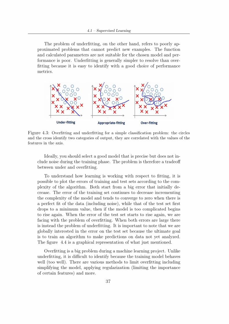
4.1 – Supervised Learning
The problem of underfitting, on the other hand, refers to poorly ap-proximated problems that cannot predict new examples. The functionand calculated parameters are not suitable for the chosen model and per-formance is poor. Underfitting is generally simpler to resolve than over-fitting because it is easy to identify with a good choice of performancemetrics.
Figure 4.3: Overfitting and underfitting for a simple classification problem: the circlesand the cross identify two categories of output, they are correlated with the values of thefeatures in the axis.
Ideally, you should select a good model that is precise but does not in-clude noise during the training phase. The problem is therefore a tradeoffbetween under and overfitting.
To understand how learning is working with respect to fitting, it ispossible to plot the errors of training and test sets according to the com-plexity of the algorithm. Both start from a big error that initially de-crease. The error of the training set continues to decrease incrementingthe complexity of the model and tends to converge to zero when there isa perfect fit of the data (including noise), while that of the test set firstdrops to a minimum value, then if the model is too complicated beginsto rise again. When the error of the test set starts to rise again, we arefacing with the problem of overfitting. When both errors are large thereis instead the problem of underfitting. It is important to note that we areglobally interested in the error on the test set because the ultimate goalis to train an algorithm to make predictions on data not yet analyzed.The figure 4.4 is a graphical representation of what just mentioned.
Overfitting is a big problem during a machine learning project. Unlikeunderfitting, it is difficult to identify because the training model behaveswell (too well). There are various methods to limit overfitting includingsimplifying the model, applying regularization (limiting the importanceof certain features) and more.
37

4 – Machine Learning: Main Supervised Characteristics and Algorithms
Figure 4.4: Correlation errors/fitting in function of model complexity: for great com-plexity of the model the test set may suffer of overfitting, while for too easy model it cansuffer of underfitting. The correct fitting is a tradeoff of the two.
4.1.4 Bias and Variance
The concept of bias and variance is closely linked to that of fitting, soit is discussed here. Bias and variance are two typical problems of themachine learning algorithms that always arise and therefore must be ableto analyze and limit. There is a tradeoff in the ability of a model tominimize bias rather than variance. If you have a lot of data available,an informal definition is as follows:
Bias :can be thought of as the error of the algorithm in predicting theoutput of the training set from which it was trained and that therefore"knows".
Variance :can instead be thought of as the worsening of prediction be-tween the training set and the test set (it is assumed that the accuracyof the training set is always better than that of the test set).
Using these two definitions is very easy to compare them with theconcept of fitting. In fact if the error on the training set is low but Ihave a big error on the test set there will be an overfitting problem andthere will be great variance. On the contrary if the error on the trainingset is big and is very similar to the error on the test set there will beunderfitting and high bias.
Finally it is possible to define a minimum bias not eliminable, in thiscase the definition of bias changes because it is necessary to take intoaccount this additional part. The unavoidable bias is not erasable by any
38

4.1 – Supervised Learning
kind of algorithm because it depends on the structure of the data. Thistype of bias is not always easy to recognize, especially in machine learningprojects that a human is not able to perform.
There are many method to reduce bias and variance, but as you cansee in table 4.1 many of them are in contrast: one reduce a problem butsometimes increase the other.
Reduce Bias Reduce Variance
Increase the model size Decrease the model sizeModify input features Reduce input features
Reduce or eliminate regularization Add regularizationModify model architecture Modify model architectureAdd more training data Add more training data
Augment complexity of the model Add early stopping in gradient descent
Table 4.1: Reducing Bias and Variance: some method are common and other are incontrast.
Mathematic Definition
To formalize the definition, it is now proposed the mathematical conceptof Bias and Variance related to the world of machine learning. Given a setof m examples each composed of n features xi and an output y , we canevaluate the performance of the machine learning algorithm through theanalysis of the convergence error between training set and real output.Thereal output y can be described by a function of x plus an error term withzero mean: y = f(x) + ε. The error we are interested to compute is thesquare of the difference between this y and the hypothesis function f(x)that is the predictive function that approximate y:
Err(x) = E[(y − f(x))2] = E[(f(x) + ε− f(x))2]
It is possible to show that the previous formula can be re-written as follow:
Err(x) = (E[f(x)]− f(x))2 + E[(f(x)− E[f(x)])2] + ε2
where the three separate terms have the following meaning:Bias2 = (E[f(x)]− f(x))2
V ariance = E[(f(x)− E[f(x)])2]
Irreducible error = ε2
39

4 – Machine Learning: Main Supervised Characteristics and Algorithms
The important thing to note is that with this definition Bias and Variancedepends on f(x) so on the selected model and on the correlated parame-ters, while ε2 is proper of the system. This means that Bias and Varianceare variable parameters that we can modify if selecting an appropriatehypothesis function while the internal error of y is not. This error de-pends on the goodness of the data and can influence a lot the final resultof the machine learning project.
Learning Curves
The learning curves are graphs of performance (y-axis) according to ex-perience or training time (x-axis). The most common in machine learningare curves of loss (cost function) or accuracy with respect to the increaseof training examples. In the same graph two curves are usually plotted,one relative to the training set and the other to the test set. In this wayit is possible to compare the evolution of the performances with respectto the variation of the experience of the algorithm based on the quantityof examples used during the training phase. In this section we decided toplot the error of the training and test sets, but later in this work you willalso see those related to accuracy that are roughly the opposite of thoseof the error.
The learning curves based on error as a function of the number ofexamples generally have a decreasing trend with regard to the test setand increasing with regard to the training set. This means that gener-ally the error of the test set decreases with the increase of the numberof examples while the error of the training set increases. At best, thetwo curves asymptotically converge around a low error and their valuesremain about constant after a number of examples of the training set. Infigure 4.5 is shown a learning curve of a model that perform well becausethe convergence is fast and the final error low.
Figure 4.5: Learning curve that seems to perform well: the two curves are convergingnear the desired value.
40

4.1 – Supervised Learning
If the behavior deviates from that of the figure 4.5 it is possible toidentify various problems that can be solved in different ways:
• High Variance• High Bias• High Bias and Variance• Model Performance MismatchIn order to identify these problems, it is necessary to be able to recog-
nize for your model a desired performance to be displayed on the graph.In the case in which the metrics of evaluation of the learning curve is theerror, it is therefore necessary to be able to estimate the error consideredacceptable for our machine learning model (e.g. I want my model to beable to fail less than 5% of the output, 5% is the desired error).
Now the possible behaviors of the learning curves will be briefly ana-lyzed:
High Variance
If you are measuring the error a model with high variance will havea big gap between test and training error. The desired performancesare still achievable because the error of the training set remains low andtherefore increasing the number of examples or using other techniques tolimit the variance the two curves will get closer and closer.
Figure 4.6: Learning curve for high variance dataset: the two curves can still convergein the range of desired performance if the model is correctly modified.
High Bias
If there are bias problems, the two curves converge rapidly and at thesame asymptote but far from the desired performance. This means thatthe test set is representative of the dataset but the model has been poorlytrained.
High Bias and Variance
41

4 – Machine Learning: Main Supervised Characteristics and Algorithms
Figure 4.7: Learning curve for high bias: the two curves behave the same and are con-verged. No more data is useful and we have to modify the model for better performance.
The two curves are quite flat and converged, far from each other andboth far from the desired performance. In this case it is necessary tochange the model or improve the pre-processing phase. If these methodsdo not work, there may be a problem of model performance mismatch.
Model Performance Mismatch Learning curves can also be used
to diagnose dataset properties and whether the dataset is representativeof the problem to be solved. A non-representative dataset does not cap-ture the statistical characteristics of the problem. The term Model Per-formance Mismatch means that the chosen machine learning algorithmbehaves very differently between training set and test set. A small differ-ence is normal because it indicates an inevitable small overfitting but ifthis discrepancy is too large it compulsory to reduce it to obtain accept-able results. We want to have small discrepancies between training andtest set so that we can compare and choose between the various modelswhich is the best. The possible causes of a Model Performance Mismatchare:
Model overfitting : usually is the more frequent cause, solutions werealready mentioned.
Quality of the sampling data: it is possible that the training or test setis not representative or that the training set does not cover all possiblecases. In this case, increasing a lot the number of examples is very usefulto cover all possible cases. To understand if we are facing this problemit is useful to analyze the statistics of the features and look for if there isgreat variance and standard deviation in the data.
Stochastic nature of algorithms : creates discrepancies in the modelscore due to a random factor (e.g. algorithm initialization) that affectsmodel accuracy. This problem can be visualized by evaluating the vari-ance of the cross validation set.
42

4.1 – Supervised Learning
Many problems with the Model Performance Mismatch can be avoidedby using a more robust test set. To understand if you are using a suitabletest set you need to perform an analysis before using it for evaluation.However, this analysis is often complex and time-consuming.
4.1.5 Evaluation Metrics
The problems related to fitting, variance and bias can be identified throughevaluation metrics, which, in addition to indicating which are the prob-lems, also make different algorithms comparable. Moreover, the samealgorithm can give good results with a certain evaluation metric, andpoor results with others. Therefore it is necessary to know all the eval-uation techniques in order to fully understand how the model is reallybehaving.
The most popular evaluation metrics are:
• Accuracy
• Confusion matrix
• Recall and Precisioin
• F1 score
• Mean absolute error
• Mean squared error
A brief discussion about these evaluation metrics are carried on:
Accuracy
Accuracy is the most classic and instinctive method of evaluation basedon the ratio between correct predictions and total number of predictions.
Accuracy =Correct predictions
Total number of predictions
A significant problem of this method of evaluation is visible when youhave very unbalanced classes in the number of occurrences, this methodof evaluation does not give useful information and you risk misunder-standings.
Example: if a machine works well in 99% of the cases and gives an erroronly 1% of the time, an algorithm that never predicts errors will predict100% negative cases (usually 0 is attributed to the major value and 1to the particular case). The accuracy, when calculated, will thereforebe 99%, which seems to be a very good value. The problem is that
43

4 – Machine Learning: Main Supervised Characteristics and Algorithms
my algorithm never recognizes a positive case, so it does not work! Forthis reason, for very unbalanced classes, other methods such as F1 score,Recall and Precision are used.
Confusion matrix
It is an array that completely defines the behavior of a model, used inclassification problems. In case of binary classification the confusion ma-trix correlates the predicted results with the real ones. Its form is shownin figure 4.2. The terms true and false, positive and negative, refer to the
Predicted Negative Predicted Positive
Real Negative True Negative False PositiveReal Positive False Negative True Positive
Table 4.2: Confusion matrix for binary classification.
goodness of the forecast after comparing it with the real output in thetest set. In detail:True Positive : positive predicted and positive real value.True Negative : negative predicted and negative real valueFalse Positive : positive predicted but negative real value.False Negative : negative predicted but positive real value.Positive is usually understood as a minority value to which we tend toassign the value 1 (in other words, the action that happens rarely has avalue of 1). You can calculate the previously defined accuracy with theuse of the confusion matrix in this way:
Accuracy =True positive+ True negative
True positive+ True negative+ False positive+ False negative
=True positive+ True negative
Total number of prediction
Recall and Precision
These are two measures based on the values of the confusion matrix. Theyare especially useful in the case of unbalanced datasets, when the mea-surement of accuracy is not adequate as described above. The definitionof precision and recall is as follows:
Precision =True positive
True positive+ False positive=
True positive
n. predicted positive
44

4.1 – Supervised Learning
Recall =True positive
True positive+ False negative=
True positive
n. actual positive
These are two measures that are often calculated for the minority classbut their definition can be modified to use it also with the majority class.
Accuracy is the reliability of the prediction. When precision tends toone for sure when the algorithm predicts a positive case the real outputwill also be positive. On the contrary when the precision tends to zeroif the algorithm predicts positive the real value will almost certainly benegative. Therefore the more the precision tends to the value one, thehigher the reliability is.
The recall instead indicates the amount of positive values found by thealgorithm on the total of the real positive values. When the recall tendsto one, the algorithm finds almost all the values that are actually positive.If it tends to zero, however, the algorithm finds almost no positive valuesamong the real ones.
There are cases where you have high precision and low recall: in thesecases you can trust when the algorithm predicts one, because it will alsobe a real positive, but there will be many unforeseen positives. On thecontrary, there are cases in which you have low precision and high recall:the algorithm predicts many positives that will actually be negatives,but on the number of forecasts the algorithm includes almost all the realpositive values. The reliability is low but it can be said to be a particularlyconservative case.
F1 Score
Since precision and recall are often in contrast, this value represents thecondensation of two metrics into one number. It is often defined in variousways but the most common method is as follows:
F1 = 2PR
P +R
Where P and R represent precision and recall values. The relation be-tween precision and recall is usually non linear, for this reason is a goodidea to use this single performance metric. Sometimes there are situatinsin which the goal is to reach a good precision instead of a high recall orvice versa. So the better choice is to apply these metrics case by case.
Mean absolute error
The metric now analyzed is again a generic metric for both classificationand regression problems that indicates the difference between the predic-tion and the real output, in practice it is a measure of the error of the
45

4 – Machine Learning: Main Supervised Characteristics and Algorithms
average prediction for all the examples of the training set. It is definedin the following way:
MAE =1
m
m∑i=1
|yi − yi| i = 1,2, . . . ,m
Mean squared error
Very similar to the previous one but it takes into consideration the squareof the difference between true output and forecast, then it averages on thenumber of examples in the training set. The advantage compared to theprevious metric is in the easy use for the search of the gradient becausewith this shrewdness of the square the calculation of the derivative issimplified a lot. The computational calculation is faster. In addition,the power of two enhances the larger errors making the algorithm moreefficient for the main losses. The form is as follows:
MSE =1
m
m∑i=1
(yi − yi)2 i = 1,2, . . . ,m
4.2 Classification Learning AlgorithmsThis section describes the main features of the most commonly used ma-chine learning algorithms concerning classification problems. The descrip-tion will be mostly qualitative, expressing general concepts and useful in-formation to understand the differences between the various algorithms.Where deemed appropriate, some mathematical concepts that are on thebasis of the algorithms will be expressed. In the literature exist numerousarticles and manuals, please refer to these for further details.
4.2.1 Logistic Regression
It is a simple and well-established classification technique. It takes itscue from linear regression, a standard technique for regression problems(output to be predicted in a continuous and infinite domain). It is basedon a hypothetical function to make predictions called Sigmoid functionor Logistic function. It is a function with real domain between zero andone and infinite co-domain. Its form is the following:
g(θTX) =1
1 + e−θTX
The Sigmoid function is defined positive, dependent on the matricial
46

4.2 – Classification Learning Algorithms
Figure 4.8: Sigmoid function: hypothesis function for logistic regression.
quantity θTX , i.e. it is a function of the features X of the examplesof the dataset once fixed the parameters θ to optimize. Returns a valuebetween 0 and 1 not a simple binary value. However, being in a problemof classification the algorithm must choose a threshold of separation ofthe two classes. Usually this threshold is set to the value of 0.5 but can bemodified to increase or not the confidence in the prediction obtained. Infact, a number close to 1 indicates that the prediction is more likely to besafe, while a value slightly higher than 0.5 is an indication of uncertaintyof the forecast. As the complexity of the θTX function increases, there aremore complex decision boundaries and a better fit of the training data,creating however the possible problem of overfitting and variance.
To find the parameters θ a modified cost function J is used comparedto the normal minimization of the square of the error between predictionand real output. This is due to the form of the cost function created usingthe Sigmoid function to make predictions, in fact if you used normally thecost function would become a non-convex function and the simple appli-cation of gradient descent algorithms would not find the global minimumbut would stop in a local minimum, resulting in poor performance. Forthese reasons the cost function becomes the following:
J(ϑ) =−1
m
m∑i=1
(y(i) log(hϑ(x(i))) + (1− y(i)) log[1− hϑ(x(i))])
Through the derivation of its gradient it is possible to find the globalminimum and therefore the appropriate parameters. Once found, thetraining phase ends and you can use the Sigmoid function to quicklycalculate future predictions.
Due to overfitting problems it is possible to modify the cost functionto find theta parameters that are less dependent on the details of the Xfeautures, this technique is called regularization.
47

4 – Machine Learning: Main Supervised Characteristics and Algorithms
Logistic regression is not the most powerful and versatile techniquebut it is certainly well structured and there are various reliable librariesthat implement it. It works well in standard machine learning problemswhere the purpose is well defined. It is very fast if there are no featuresdisconnected from the output or similarities between features (indepen-dent features). It is susceptible to overfitting problems and requires wellformatted and linearly separable data.
4.2.2 Naive Bayas
Unlike the previous one, this is a probabilistic method based on the Bayestheorem. First of all we calculate the probabilities of obtaining an out-put 0 or 1, based on the training dataset, then we individually correlatethe features with the output, that is according to the value of a featurewe calculate the probability that the output is 0 or 1. We repeat thisoperation for all the features, then we make cross correlations betweenthe probabilities just calculated. In other words we multiply the variousprobabilities feature by feature obtaining a general value index of theprobability of that sequence of features with respect to the output. Themore features you have and the more diversity of possibilities you havefor each features, the more complex the calculation and cross-referencingof data becomes. The probabilities obtained must then be normalizedaccording to the recurrence of the features and their values.
In mathematical terms we can say that given a problem of classifica-tion it is represented by n featuresX (they must be independent for Bayesproperty). The model assigns a probabilistic outcome to each Ck for eachpossible K outcome. If we are in binary classification the outcomes areonly two (0 or 1). In formula:
P (Ck|x1, x2, ...xn)
Using Bayes’ probabilistic theorem rewrites the previous formula in thisway:
P (Ck|x) =P (Ck)P (x|Ck)
P (x)
That is, in Bayesan terminology:
Posterior =Prior ∗ Likehood
Evidence
Evidence is a constant that depends on features data, it is a normaliza-tion constant. Prior * Likehood can be rewritten (assuming indipendent
48

4.2 – Classification Learning Algorithms
features) as:
P (Ck|x1, x2, ...xn) = P (Ck)n∏i=1
P (xi|Ck)
The Naive Bayes classifier combines this probabilistic model with certaindecision rules based on the value of probability. This creates an algorithmthat provides an output based on the probability calculated with theBayes theorem. It is therefore assigned y = Ck for a certain k based onthe following rule:
y = argmaxK∈{0−1}P (Ck)n∏i=1
P (xi|Ck)
There are various versions and extensions of this classifier such as Gaus-sian Naive Bayes, Multinominal Naive Bayes, Bernulli Naive Bayes,. . .
A theoretical limitation of this algorithm concerns the independenceof features. In practice, in fact, this hypothesis is difficult to achieve.However, various tests have shown that even if this hypothesis is notguaranteed, the model often behaves well. A disadvantage is the behaviorof the algorithm towards new features, as these will be assigned a zeroprobability and you can not make a prediction. So it needs well-formatteddatasets and large enough to cover all cases. It is often used in real timeapplications, for multiclass classification, text classification, social mediaanalysis, recommender system.
4.2.3 Support Vector MachineSupport Vector Machine can be seen as an extension of logistic regression.Its cost function is very similar to the one previously analyzed. In fact,it is a piecewise approximation of the logarithmic values within the costfunction. Its structure becomes:
J(θTX) = C
m∑i=1
(yicost1(θTX) + (1− yi)cost0(θTX)) +
1
2
n∑j=1
θ2j
where cost1 and cost2 are the piecewise approximations of the logarithms.Moreover, the constant C is the term of regularization and the part 1
m
is no longer present in the minimization of the cost function. Unlike thelogistic regression which has only one decision threshold to obtain theprediction 0 or 1, the SVM has limit values beyond which the predictioncan only be 0 or 1: {
θTX ≥ 1→ y = 1
θTX ≤ −1→ y = 0
49

4 – Machine Learning: Main Supervised Characteristics and Algorithms
There is an additional safety factor between -1 and 1 to be sure of theresult. While in logistics the only threshold was around zero.
SVM is defined large margin classifier because it always leaves thegreatest margin in the choice of the decision boundary, this increases therobustness of the algorithm, it is always chosen the line with more marginwith the same fitting. This property is graphically visible in the figure4.9.
Figure 4.9: SVM: large margin classifier. The selected boundary is the farthest from thedata.
SVM works by defining a similarity function that associates a valuebetween 0 and 1 to each landmark-example pair. Each example is chosenas a landmark, so calculating the similarity function creates regions witha wide margin to identify areas where the output is 0 or 1. That is, eachexample becomes a nucleus from which the similarity with the other nu-cleus are defined. The similarity function can be more or less complex.Some examples are Linear Kernel, Gaussian Kernel, Polynomial Kernel,String Kernel and others. . . Due to its cost function it is possible to opti-mize the computational calculation making it fast and efficient. In otherwords, the SVM is based on the idea of finding a hyperplane that bestdivides a set of data. The term "support vector" identifies the points(examples) closer to the hyperplane, if they are removed or moved theymodify the position of the hyperplane. The margin is therefore the dis-tance from the "support vectors", these distances define the position ofthe dividing plane. The hyperplane can be linear or non-linear using thekernel idea.
The advantages of the SVM are: effectiveness in large spaces, memoryefficiency, versatility in the choice of the hyperplane, accuracy.
50

4.2 – Classification Learning Algorithms
4.2.4 Random Forest Classifier
This algorithm is based on the concept of decision tree. A decision treecan be considered as a predictive model for making classifications. It hasa hierarchical structure formed by a series of ramifications that convergemore or less slowly towards a result based on a series of decisions imposedduring the branching of the tree. The main characteristics of a decisiontree are:
Entropy : it is a measure of the unpredictability of the system, it is onthe database itself.
Information Gain :when a decision is taken the database is divided ineven more little parts, the entropy is reduced. The information gainis a measure of the entropy reduction after a node.
Leaf Node : it is th last node of the tree, where the decision is taken.Here the entropy is minimum and the classification estimation is per-formed.
Decision Node : nodes where the divisions are taken and the databaseis splitted into subsets.
Root Node : it is the top decision node, the database here is completeand the entropy is maximum.
Decision trees therefore lead to a result based on successive choicesthat tend to decrease the entropy of the dataset. They are usually usedfor classifications, but if carefully imported they can also be used forregressions.
A single decision tree is usually characterized by great variance, sowe use a technique that increases the security of the choice called Bag-ging. Bagging (or Bootstrap Aggregating) is a resampling technique.The data is sampled with repetition several times, thus obtaining manydifferent datasets. After which many decision trees are created, one foreach dataset and finally the average of the results thus obtained is cal-culated or the most recurrent result is chosen. These measures greatlyreduce the variance and make the result more reliable.
The algorithm of Random Forest is based on the idea of Bagging, butimproves it because the various trees are not correlated each other. Inother words, the various re-sampled datasets are scrolled between them,thus obtaining a wider safety margin and a greater reduction of the vari-ance. The term "forest" refers precisely to the fact that various decisiontrees are used. The algorithm uses them to make classifications betweenindependent resampled datasets. The chosen result is the most repeated,the one that happens most frequently in the forest. The important thing
51

4 – Machine Learning: Main Supervised Characteristics and Algorithms
to underline is that each dataset has a different decision-making modelbased on the characteristics of its own features.
The random forest algorithm has some main advantages: the use ofmany decision trees limits the problem of overfitting. Due to the simplic-ity of the model, the algorithm is fast in terms of training time. It runsefficiently on large datasets and works well even in case of datat miss-ing. So it is an excellent algorithm when you do not have well structureddata or not easily correlations because its great versatility finds the rightdecision boundary.
Figure 4.10: RFC: general structure of a Random Forest Classifier. First the dataset isdivided in independent subset, each of them make a prediction based on their decisiontree. The final outcome is a joining of all the decision tree results.
4.2.5 Nearest NeighborIt is an algorithm that is based on the similarity of the characteristics ofa certain data that you want to classify with respect to k known elementscloser to it. Once fixed the k some regions are defined in the space of thefeatures where an element for proximity to the other known elements islabeled according to the characteristics of the dominant elements of thatspace. Each element within a known region is immediately labeled. If theclassification is binary (only 0 or 1 ) it is better to select an odd valueof k to make sure you always have a majority in a given region of space.For the same reason k should never be multiple of the number of classes.The main disadvantage of this algorithm is the complexity of searchingfor the nearest elements for each new example.
The operation process of this algorithm is easily visualized graphicallyin the case of only two features in the database. In the figure 4.11 youcan see how the regions of the classification space change as the value ofk increases.
52

4.2 – Classification Learning Algorithms
Figure 4.11: KNN: classification changes basis on different k. The lighter color indi-cates a lower reliability of the solution, i.e. those regions have neighbors of not uniqueclassification.
This algorithm is very powerful when there are large non-linearitiesin the structure of the dataset, in fact the KNN algorithms are basedon similarities and can create very complex decision boundaries, differ-ently from any mathematical formula in other models. The result is anincredibly flexible algorithm, especially if the value of k is low. In thiscase, however, the fit of the data is too precise and you risk running intothe problem of overfitting because the decision boundary is fragmentedand too detailed. On the contrary, if k increases the decision boundarybecomes more and more defined.
As we have understood, choosing the appropriate value of the param-eter k has a great influence on the performance of the algorithm, in factoften entire regions change classification according to its value. To chooseit correctly there are some general rules that should be followed. Usuallychoosing k as the square root of the number of examples in the datasetgives pretty results, but it should always be rounded to the odd numbernearest the exact square to avoid possible confusion between two classesof data.
In the case of large datasets the value of the parameter k will be high,this considerably increases the complexity of the algorithm and slows itdown. For this reason it works best on small or medium datasets. KNNworks well on well-labeled, noise-free databases. It is also defined as lazylearner : doesn’t learn discriminative function from the dataset.
Mathematically, the similarities on which the algorithm is based arecalculated on the Euclidean distance in the multidimensional domain ofthe features of dimension n. A general structure of this distance is the
53

4 – Machine Learning: Main Supervised Characteristics and Algorithms
following:
d(i) =
√x(i)21 + x
(i)22 + · · ·+ x
(i)2n
However, it is possible to use different distance formulas in order to givemore or less importance to some features. It is evident that as the num-ber of features n, number of examples m and value of the parameter ofneighbors k increases, the complexity increases considerably in the calcu-lation of the distance and therefore in finding the classification regions.Any algorithm that calculates measurements from features always needsto normalize the data before performing the calculation. This is necessaryto give each feature the same importance.
4.2.6 Neural Networks
Neural networks are a very powerful tool for machine learning. In recentyears they have become increasingly popular due to the fact that thecomputing power needed to manage them is now available. The neuralnetworks are in fact a tool known for decades but really never used untila few years ago because of the scarcity of computational resources of theyears of the 900’.
The neural networks are so called because their structure tries to em-ulate the human brain. Basically, in fact, they are made up of neuronsinterconnected among them by means of dentrites and axons. The den-trites receive the various inputs from the other neurons, while the axonis in charge of transmitting the processed output, which depends on theinputs received. Therefore various complex connections are formed, theseconnections create the network. Each input to the cell is weighed andtherefore the importance changes through appropriate coefficients to bedetermined during the training phase of the network.
Technically, an artificial neural network is composed of three types oflayers:
• Input Layer
• Hidden Layer
• Output Layer
In the simplest cases there are only three levels, but for more complexnetworks the number of hidden layers can be greater than one, while inputand output layers are always single. If the classification to be carried outis binary, the output layer is composed of only one cell able to estimateif the output is zero or one, while for multiclass classification the outputlayer is composed of several cells.
54

4.2 – Classification Learning Algorithms
The learning of a neural network involves, after having fixed the struc-ture of the network, to find the parameters that weigh the various signalscarried by the network. During the training, the examples are analyzedindividually, as the machine processes the outputs, it proceeds to correctthem to improve the responses by varying the weights.
The training mechanism is a continuous iteration for all examples ofthe binomial forward propagation and back propagation. It starts withrandom weights, propagates directly to the predicted output, calculatesthe error with respect to the actual result, and performs back propaga-tion to calculate the error at each step of the network. In this way, thecoefficients that cause the error are calibrated. Also for this algorithmwe try to minimize the cost function related to the errors. This processis a complex process that can be quite slow. However, the efficiency of awell trained neural network is usually very good and the results are oftenmore satisfactory than those of other algorithms.
The user of the neural network libraries does not have to worry aboutimplementing propagation. Its task is to select the appropriate networkstructure in terms of size, number of layers and number of neurons. Thisis a delicate and not easy task. It is a good idea to always start froma single hidden layer and try to increase the number if the performanceis not satisfactory. More hidden layers must have more or less the samenumber of neurons, this number must be comparable with the number ofinput features for each example, to not create an unbalanced network.
in figure 4.12 is shown a typical structure of a neural network at severallevels for binary classification.
Figure 4.12: Neural Network: a typical structure: the network shown has three inputfeatures, a single binary output and three hidden layer equal is size and comparable withnumber of features.
The advantages of a neural network are the high parallelism thanks
55

4 – Machine Learning: Main Supervised Characteristics and Algorithms
to which a lot of data can be processed in a short time, the toleranceto faults, the tolerance to noise, the self-adactivity to data change. Thelimits, on the other hand, are linked to the fact that it is not always clearhow the network arrives at the results, so the algorithm behaves like ablack box. In addition, the training period is long due to the complexityof the algorithm.
4.2.7 Linear Discriminant Analysis and Principal Com-ponent Analysis
These last two algorithms are not classifiers and therefore are not usedto make predictions of the results. The objective is to discard irrelevantor less relevant informations to the problem of interest.They are used inthe preprocessing phase to reduce the number of features and compressthem to make the classification algorithms more efficient and make thedata well separable so as to reduce overfitting.
LDA and PCA are both linear transformation techniques. PCA is anunsupervised learning algorithm that identifies the direction of the prin-cipal components that maximizes the variance of the database (preservepattern information to the fullest possible extent). LDA is instead a su-pervised learning technique that finds the direction that maximizes theseparation between classes to facilitate classification (favours dimensionsthat discriminate against classes ).
The structure of the LDA process is as follows:
1. Calculation of separability between classes.
2. Calculation of the distance between the class average and the exam-ples for each feature.
3. Build the smallest dimensional space that maximizes the first stepand minimizes the second.
4. Project the original data into the created subspace.
Some of the disadvantages of the LDA analysis are the low efficiencyin small databases and the problem related to the non-linearity of theinitial features. If linearity is not guaranteed, the LDA analysis cannotfind the subspace to reduce features dimension. This problem can bepartially solved by using the kernel, similar to SVM kernel technique.LDA analysis is often used in speech recognition and in many medicalapplications where features are linearly separable.
The PCA aim instead, is to reduce the number of variables describinga dataset to a smaller number, limiting the loss of information as much as
56

4.3 – Regression Learning Algorithms
possible. This happens through a linear transformation of the variablesthat projects the original ones in a new Cartesian system in which thenew variable with the greatest variance is projected on the x axis, secondaxis for second size of the variance, and so on. Unlike other linear trans-formations of variables practiced in the field of statistics, in this techniqueare the same data that determine the vectors of transformation, and thatis why the PCA is defined as a technique of unsupervised learning.
In figure 4.13 a representation of the PCA and LDA application isshown for a dataset with two featuresx x1 and x2. The black segment thatidentifies the PCA solution is the hyperplane on which projecting the pat-terns (regardless of their class) we keep as much information as possible.The green segment that identifies the LDA solution is the hyperplaneon which, by projecting patterns, we are able to distinguish between thebetter the two classes (red versus blue patterns).
Figure 4.13: PCA and LDA representation in a two features size database: the greenand the black lines are a compression from 2D to 1D for LDA and PCA. The objectiveon LDA is to separate the classes, the one of PCA is to retain the maximum amount ofinformations.
4.3 Regression Learning Algorithms
As previously done for classification problems, in this section we will men-tion the main algorithms of machine learning for regression problems, thatis with the desired output to be searched in a continuous domain.There
57

4 – Machine Learning: Main Supervised Characteristics and Algorithms
are other types of regression algorithms that can be used in certain par-ticular cases when the most common, mentioned here are not suitable forthe problem to be solved. In this section we list the most important.
4.3.1 Linear Regression
Linear regression is the first and basic concept of machine learning for re-gression problems. As already mentioned above, it has such a hypothesisfunction:
hϑ(x) = ϑ0 + ϑ1 ∗ x1 + ϑ2 ∗ x2 + · · ·+ ϑn ∗ xn
As you can see is a linear prediction formula in the coefficients andin the inputs. The coefficients ϑ have to be estimate and the features xare the input informations taken from the database. The cost function tooptimize to find the best ϑ to have minimum error is instead:
J(ϑ) =1
2m
m∑i=1
(hϑ(x(i))− y(i))2
As you can see the cost function tries to minimize the error betweenthe prediction made by the hypothesis function with certain parametersand the real output desired. This means that the parameters must bechanged several times before reaching a satisfactory result. The selectionof the parameters therefore takes place in an iterative way according tothe following formula:
ϑj = ϑj −α
m
m∑i=1
[(hϑ(x(i))− y(i))x(i)j ]
Here there is the introduction of a new parameter, the so-called learn-ing rate α. Tuning this parameter change the velocity of the conversionand in its accuracy. A big value of α may create problems of oscillationsin the convergence or even divergence, whie a too little value imply greatprecision but very slow convergence so the number of iterations requiredto converge at the minimum of the cost function will be huge. Deter-mination of the learning rate parameter is essential for a good choice oflearning parameters.
In the figure 4.14 it is visible a fitting of the data with linear regres-sion, the figure shows a two-dimensional representation. It is possible toimagine a straight line in more dimensions to the increase of the featuresthat makes the solution no longer graphable.
58

4.3 – Regression Learning Algorithms
Figure 4.14: A typical example of linear regression fitting in 2D.
4.3.2 Polynomial RegressionThe polynomial regression has the same cost function as the linear re-gression from which it starts. The objective is always to find the bestcoefficients that minimize the error between prediction and true output.What changes is the form of the hypothesis function. The input featuresare now interpolated obtaining a polynomial between degree greater thanone among the features while the linearity of the coefficients remains. Infact it would be better to define this kind of algorithms as linear regressionwith polynomial features.
It is possible to have any degree of interpolated features, the more thedegree grows, the more the number of total features will be. For example,think of a machine learning problem that involves only 2 features. Thehypothesis function of a normal linear regression is:
hϑ(x) = ϑ0 + ϑ1 ∗ x1 + ϑ2 ∗ x2
while for a polynomial regression grade 2 we will have:
hϑ(x) = ϑ0 + ϑ1 ∗ x1 + ϑ2 ∗ x2 + ϑ3 ∗ x21 + ϑ4 ∗ x22 + ϑ5 ∗ x1 ∗ x2
and grade 3 becomes:
hϑ(x) = ϑ0+ϑ1∗x1+ϑ2∗x2+ϑ3∗x21+ϑ4∗x22+ϑ5∗x1∗x2+ϑ6∗x31+ϑ7∗x32+ϑ8∗x21∗x2+ϑ9∗x1∗x22
As you can see the complexity of the hypothesis function grows a lot assoon as the degree of polynomial interpolation rises. For what has been
59

4 – Machine Learning: Main Supervised Characteristics and Algorithms
said so far, if the selected degree is high, the fitting will be more and moreprecise with a great risk of overfitting. Moreover, the number of featuresincreases exponentially, so the computational calculation is a determiningfactor in the polynomial regression.
If you have only one feature you can also represent this hypothesisfunction in a 2D plane as shown in figure fig:regpol where the interpo-lation no longer generates a straight line but a curve that approximatesthe real values.
Figure 4.15: Polynomial regression, the hypothesis function is now a curve.
4.3.3 Ridge and Lasso RegressionThese regression algorithms are based on linear or polynomial regressionwith the addition of a term in the regularization cost function. Thisdevice has been thought to avoid the problem of overfitting, therefore theterm has the function to give less importance to the coefficients in thehypothesis function of certain terms, so that the fitting of the data doesnot lead to the above mentioned problem.
In detail, the Ridge regression has the following cost function:
J(ϑ) =1
2m
m∑i=1
(hϑ(x(i))− y(i))2 + λ
m∑i=1
ϑ2i
λ (lambda) is defined as the tuning parameter, which multiplied by thesum of the squared coefficients (excluding the intercept) defines the penaltyterm. It is evident that having a λ = 0 means not having a penalty inthe model, that is we would produce the same estimates that with theminimum squares. In another way having a λ very large means having a
60

4.3 – Regression Learning Algorithms
high penalty effect, which will bring many coefficients to be close to zero,but will not imply their exclusion from the model. The ridge regressionmethod never allows the exclusion of estimated coefficients similar to 0from the model. This lack, from the point of view of the accuracy of theestimate, may not be a problem. A problem connected to this limit is onthe side of the interpretability of the coefficients, given the high numberof predictors.
The lasso method (least absolute shrinkage and selection operator)fills the disadvantage of the ridge regression. It allows the coefficientsto be excluded from the model when they are equal to zero. It can benoticed that the formula of the ridge regression is very similar to thatof the lasso, the only difference consists in the structure of the penalty,in how much it is necessary to calculate the summation of the absolutevalue of the coefficients:
J(ϑ) =1
2m
m∑i=1
(hϑ(x(i))− y(i))2 + λm∑i=1
|ϑi|
As in the ridge regression the lasso method forces the estimated coeffi-cients towards zero but, the absolute value present, forces some of themto be exactly equal to zero.
In general, it can be expected that ridge regression will do a betterjob when the number of predictors is high, and at the same time that thetime frame will do a better job when the number of predictors is small.
4.3.4 Support Vector Regression
The support vector machine (SVM) method already seen in the regressionalgorithms part can also be used for part and regression while keeping thecharacteristic part of the massive margins intact. If used for regression itsname becomes Support Vector Regression (SVR) with some differencescompared toSVM: it is impossible to estimate a number with respect to aninfinite range of possibilities so we use a range within which the solution isdefined as ideal. The main idea is always the same, however, to minimizethe error by finding the hyperplane that maximizes the margins, takinginto account a certain rollerance in the error as just said.
Even the kernel function has the same function of transforming thedata into a higher dimensional feature space to make it possible to performthe linear separation.
61

4 – Machine Learning: Main Supervised Characteristics and Algorithms
Figure 4.16: Support vector regression with the usage of tolerance range for finding themaximum margin.
4.4 Supervised Algorithm Choice
There are many types of machine learning algorithms and many librariesare able to implement them in a performing way. The choice of algorithmto use is not obvious, because each algorithm has strengths and weak-nesses and there is no better model than the others but depends on eachsituation.
Given the large number of algorithms available, it is necessary tocreate a selection process through 2 phases: before and after training inorder to train a limited number of algorithms based on the characteristicsof the dataset.
4.4.1 Choose feasible algorithms
Before training the algorithms it is already possible to partially under-stand which of the various possible choices will be those that will workbest for our dataset. This group of algorithms is based on the character-istics of the dataset. The parameters to select them are:
• Linearity of the database
• Missing values in the dataset
• Data repeatability
• Examples and features number
• Number of algorithm parameters
• Class imbalance
62

4.4 – Supervised Algorithm Choice
Linearity of the database
Some algorithms of machine learning use hypothesis of linearity, it ismeant that the classes or the features of the database are separable froma linear function like a straight line or from a space o hgher dimensionsequivalent and linear. This hypothesis is difficult to ascertain and oftennot applicable to real cases. It happens that the features are dependentand not separable, for this reason the linear algorithms obtain not goodresults. More realistically, the data needs polynomial interpolations orvery complex decision boundaries. However, a high degree of polynomialinterpolation is very expensive at a computational level and may thereforemake a probabilistic method preferable to an exact one because of the highcomplexity required.
Linear algorithms are however an excellent starting point to under-stand how the dataset is structured and to direct the choice to morecomplex models, avoiding trying to find the best model with a bruteforce technique.
Missing values in the dataset
A very common feature in databases is the presence of missing valuesbetween the data. These are due to different phenomena such as thediversification of the examples in the dataset, data sampling errors, er-rors during the pre-processing phase,. . . It is very important to take into
account the missing values because some algorithms work badly or donot work at all in the presence of missing values between the data. Thisproblem can be solved in two ways: The pre-processing phase is extendedby deleting examples or modifying data; the choice of an algorithm thatis less sensitive to missing values.
In both cases the solution is not optimal because you lose time andyou generally get worse solutions than you would get with a homogeneousdataset without missing values. The techniques of treatment of thesevalues are many and if necessary they will be discussed when they occur.
Data repeatability
Any algorithm to work well requires that the outputs to be predicteddepend on features very similar to those with which the algorithm wastrained. However, some models are more sensitive to changes in the inputdata to be predicted. These make them adaptable to the training set butwith a poor behavior on the test set and future predictions. This is due tothe more or less important change in input data over time. It is therefore
63

4 – Machine Learning: Main Supervised Characteristics and Algorithms
better in these cases to select an algorithm with worse performance onthe training but with greater versatility and repeatability of accuracy,this increases the reliability of the output.
Another solution if you want to keep the same high-performance algo-rithm in your training is to increase the training time and data to cover allpossible cases. Finally, the best performance is obtained by making thealgorithm self-learning over time, i.e. using the prediction data as subse-quent data to perform a new training by increasing the total dataset andadding information from the new examples. With this care the algorithmadapts to the changes that can occur in time and the output remainsreliable over time. The cons is that this continuous training requireshigh computational costs to keep the model up to date, this is often notacceptable during a normal application of the model.
Examples and features number
The size of the database is relevant not only for the training time but alsofor the intrinsic ability of an algorithm to properly manage a large amountof information. For some algorithms it becomes difficult to extract infor-mation on what are the relevant features causing overfitting problemsthat are difficult to solve and identify. In the same way there are oppo-site problems related to data underfitting if the size of the database is notadequate. In any case, it is necessary to act on the modification of thefeatures, using techniques of regularization or extension of the features.Some algorithms are better then other to extract these informations with-out modifying the database and this can imply less time to dedicate atthe preprocessing phase.
Number of algorithm parameters
The parameters of the algorithms are those coefficients that characterizethe setup of the model. An algorithm with many parameters is moredifficult to optimize than one with few, and requires a lot of experienceto be used. In general, an algorithm with several parameters is moreflexible and adapts well to many cases, but it is difficult to find the rightcombination of these parameters to achieve the best possible performance.
Class imbalance
For classification, an unbalanced dataset guides the user to the algorithmsthat will perform best. Usually having a great imbalance between theclasses we tend to use more robust algorithms specifically designed for
64

4.4 – Supervised Algorithm Choice
this function. Algorithms based on research trees are very powerful inthese conditions.
4.4.2 Best algorithm selectionOnce you have chosen the group of algorithms that you think can bestbehave with the dataset you have, you can train these algorithms andevaluate which is the best of them on the basis of:
• Performance
• Training time
Performance
One of the most important features of a machine learning algorithm isthat it predicts data well. This is the main purpose of any of such project.Performance evaluation is done by using a test set to simulate the algo-rithm’s task, i.e. predict results before they occur. Thanks to the use ofthe test set it is possible to extract the evaluation metrics that quantifyin a simple and intuitive way the goodness of an algorithm. They alsomake it possible to compare different models so that you can choose theone with the best performance. For further information, please refer tothe chapter 4.1.5 where the main ones are discussed in detail.
Training time
It is another characteristic to take into account, especially when compar-ing various algorithms. If you have to do several tests and trials it is agood idea that this time is limited in order to evaluate the algorithm.Moreover, there is often a constraint imposed by the project on the timefor elaboration. This time is closely related to performance but somealgorithms, especially those based of probabilistic models, may take ashort time to optimize the parameters and still obtaining good results.The training time factor can limit the possibilities for a decision of certainalgorithms especially for very large databases because even slightly betterperformance can lead to long computational calculations not acceptable.
65


Chapter 5
Error Prediction: DataPreparation
This chapter and the following one are dedicated to the problem of errorprediction. As mentioned in the chapter 1.2 the problem to be solved isto try to predict abnormal machine stops and badly finished parts. Thesolution chosen involves the use of machine learning algorithms to findcorrelations between the inputs provided to the machine. To do this,the first phase of work is to reconstruct the series of inputs that can bedecisive for a possible failure of the machine. This will be discussed inthis chapter, while in the next we will test various algorithms to find theone that best suits the problem.
In details we start describing the creation process of a single largetable of cuts. Each cut event will be associated with all other relatedevents in such a way as to extend the features of the data and add all theinformation obtainable from the raw database described in the chapter 3.From this unified table it will then be possible to easily select subsectionsrelated to the machines concerned.
In the second part we will look for information about the correlationsbetween features, trying to identify the most similar and dependent ones.Ensuring independence between features is essential to avoid repetition,lighten computational calculation and get better results from machinelearning algorithms.
Finally, a statistical analysis will be carried out between the features ofeach machine. This will eventually justify a separation of the applicationof machine learning algorithms for individual machines and will then alsodefine the subsections for best results.
In this chapter and in the following ones we will take for granted the
67

5 – Error Prediction: Data Preparation
knowledge of the Jupyter Notebook programming environment, as wellas of the Python programming language and of the main libraries usedfor data management, that is Pandas and NumPy. Further informationon the working environment is presented in appendix one, chapter 9.
5.1 A bug in manual mode data collectionA problem come up when plotting the number of occurrences of a badlyfinished cut according to the CutLength feature. To do this, we filteredthe extended database by taking only the lines containing a BadTermi-nated_MC==1 and we used the .hist() method of Pandas to create thehistogram. In this study all data of the three machines were used.
In figure 5.1 it is visible the diagram of the occurrences of a terminatedbadly in function of the length of cuttings given as input. As you cansee, there are 2 cutting lengths in which many errors are generated, thatis, when the cut is set to 0mm and 3200mm , while the rest of the errorsare distributed over all the other lengths.
Figure 5.1: Bad terminated cuts occurrency in function of cut length: two peack areclearly visibles where the errors occurr.
Two further subgraphs have been obtained from the previous one,they are visible in the figure 5.2. By dividing the manual steps from theautomatic ones, in this way it has been discovered a very important factthat changes the study conducted. In the graph of the automatic steps
68

5.2 – Data merging
the peak on the length 3200mm remains, this peak is due to the fact thatthe glass sheet have dimension in height of this measure, therefore it is thedimension more cut and the more recurrent, and so it is on this measurethat the greater part of the errors is concentrated. The manual step graph,on the other hand, has only one value for which the errors occur, namelythe value of CutLength==0. It was thus discovered that the softwarethat generates the badly finished events for manual cuts contained a bugand the errors were only sent when the selected measurement was zero,without taking into account all the other potential bad situations thatcan occur in the reality of the problems.
The main consequence is that it is not possible to use thesteps made in manual mode in the machine learning algorithmbecause they are buggy. From now on, therefore, the manualsteps identified by the feature StepManual_C== 1 will be dis-carded. All the graphs and tables will refer from here on onlyto cuts made in automatic mode.
Figure 5.2: Automatic and manual occurrency of bad terminated cuts: from this graphwas discovered a bug in manual mode data sending. From now on manual mode data areno more used.
A further check of the above is visible in the figure 5.3 where yousee the same histogram graph of the occurrence of errors as a functionof the cutting length divided by customers. This shows how the bug iscontained in the software of each machine analyzed, as the badly finishedoccur daily at different lengths even if the step is manual.
5.2 Data mergingThe term data merging means the union of several datasets into one,extended, containing information from all the sets that compose the
69

5 – Error Prediction: Data Preparation
Figure 5.3: The discovered bug affects all the clients: no error registration for cut lengthdifferent from zero in manual mode operations.
database. This process is necessary when you have multiple sources ofinformation, raw data or multiple separate tables for storing data. Youcan divide this process into three possible groups:
Extend examples : Merging in this way extends the number of exam-ples, i.e. the length of the table. This method of unification is alsocalled "hanging new data". It is assumed, in this type of merging,that the tables to be merged have the same variables and that themeaning of the columns is the same for both tables. It is also goodto check that the various examples (the rows, the entries of a table)are not repeated in the various tables to be merged, otherwise it isnecessary to remove the duplicates after merging the data.
Extend the number of features : Extending the number of variablesrequires some correlation between features of the two tables to bemerged. Without a proper correlation it is impossible to merge them.Normally this type of merging is done on the basis of table indexes oron the value of some feature that is repeated in both datasets. Theoutput of this merging is an extension of the columns with respect tothe starting datasets. The entries remain the same but the amountof information for each example increases. Also in this case youwill eventually have to delete the related features to avoid linearcorrelations between them.
Associate features uing look-up : This type of merging is the mostcomplex and is used when you have incomplete datasets to combine,i.e. with different features and different information contained. Thereis not an equal column for merging, only a few data in scattered orderare the link between the two tables. The method of association istherefore done through some values of one or more features presentin both datasets, or through an algorithm that can identify for each
70

5.2 – Data merging
example of the first set exactly a value of the first set. This impliesthat this merging can take place between tables of different sizes aslong as there are direct or indirect correlations between some featuresof the tables.An example is the association of a geographical region (based on thezipcode) to the examples of a table where each entry corresponds tothe districts of a city. The table to be extended contains informationabout the neighborhood and the zipcode of the city. Another tableinstead correlates zipcode and region of origin. It is not certain thatall the zipcodes of the second table also belong to the first and noteven the opposite if the second table is incomplete. But surely ifthe zipcode of the two tables coincides you can assign the first tableto the region of belonging, so as to know the location of a certainneighborhood in the corresponding region. This merging method isa kind of cross association between the two tables.
In our case the second and third merging methods will be used, as we donot need to first that extend the examples because for this work they arealways all contained in the database described in the chapter 3.
5.2.1 Basic ideaHere are described the guidelines of the process that will be analyzedtechnically and in detail in the following sections. What you want to getis an extended table for the events of type Cut containing informationof other events of Step, TypeOfGlass, Glass, Session. The method ofcorrelation of the tables is different for each event and will be describedlater. The desired output is a table with m examples (correspondingto the number of examples of the cutting event) and n features. The nfeatures are due to the sum of the single columns coming from each event.Mathematically:
n = ncut + nstep + nses + ntype + nglass
where each ni is a subsection of the total number of features presentfor event i. If you look at the chapter 3 you will see that each exampleconsists of a set of features, only the most relevant of them are selectedto extend the table of cuts.
In table 5.1. you can have a schematic graphical display of the desiredoutput, with the features from the events just described. It is importantto note that the unified table has as its starting point the table of cuts andextends based on this. So the output can be defined as an extension ofthe table of cuts that collects much more information from other events.
71

5 – Error Prediction: Data Preparation
Cut Event Step Event Session Event TypeOfGlass Event Glass Event
1. . .ncut 1. . .nstep 1. . .nses 1. . .ntyp 1. . .nglass
n total features
Table 5.1: Schematic shape of table obtained after data merging.
5.2.2 Cut tableAs defined in the basic idea,it is necessary first create a table of cutevents. This table is created by extracting only this type of event from thedatabase based on the EventCode. You then delete the unused databasecolumns and rename the remaining ones to give them explicit meaning.Finally, extract the information from the mask in EventData2 and insertit into the new features as boolean variables. Information about this eventcan be found in the paragraph 3.1.4.
The figure 5.4. shows this procedure of creating the table of cuts ina flow chart easy to understand. In a real approach I used Python withthe library Pandas for managing dataframes. TEvents contains part ofthe entire database from a prefixed date, so the TEvents dataframe isstructured exactly as described in the chapter 3.
5.2.3 Associate Step eventTo associate step events to the newly created cut table, you must alsocreate a suitable step table. Not all the steps, however, are related to acut event, only the steps of type StepVsxCut5X8 and StepVsxDiagonal-Cut5X8 (see table ?? for further details), this is due to the fact that,as the software that manages and sends the events to the database isstructured, every time a step of the type StepVsxCut5X8 and StepVsxDi-agonalCut5X8 takes place, a cut event is also recorded. In these cases thetwo cut and step events are sent together at the same time. In practicethe two events are recorded in the same second but with a difference of afew milliseconds. This information is the basis of the association betweenthe two tables, in fact, based on the hypothesis that a machine can notdo more than one cut per second, you can truncate the datetime of thetwo events in the range of seconds and use them as a comparison betweenthe events to do the merging of data.
This procedure can lead to a slight loss of data if the cut and stepevents differ by several milliseconds so that their truncated DateTimesper second differ. If the number of seconds is different, the merging is
72

5.2 – Data merging
Figure 5.4: Process of cut table creation in flow chart.
unsuccessful and both parts are discarded. From the verifications carriedout the loss of data is negligible.
In figure 5.5 you can see the flow chart tocreate the step table whenthe step type is StepVsxCut5X8 or StepVsxDiagonalCut5X8, the othercolumns of the table are those extrapolated from TEvents and defined inparagraph 3.1.3, some of them are discharded or renamed for an easierusage. As explained before the column DateTime will be used to mergewith theProcessorID.
In the figure 5.6 there is the steps to create the extended table Step+ Cut. The merging keys (i.e. the values to be compared) are the Pro-cessorID of the machine that generates the event and the DateTime ap-proximated to the seconds. In the real implementation code aninner joinis executed: only when both keys coincide a new entry in the extendedtable is created. This means that in the new table you will never havemissing values due to the non-association of the two table entries. Thenegative aspect is a slight loss of data considered not to be influential.
73

5 – Error Prediction: Data Preparation
Figure 5.5: Step table creation flow chart.
5.2.4 Associate other events, the example of SessioneventWhat will now be explained for the session event is also valid for the otherTypeOfGlass and Glass events.
To insert the information about the session in the previously createdcut + step table, a separate table is used, containing only informationabout this event code. The session event extrapolation program and thecreation of the relative table is very similar to the previous and its flowchart is omitted. Remember that the meaning of the features for thisevent is described in the chapter on the database in paragraph 3.1.1.
To join these new informations coming from the Session it is not pos-sible to perform an inner join to extend the table (like before betweenStep and Cut). This is due to the fact that the number of Session eventsis much lower than the number of cuts and there is not correlation oneby one. Remember that the Session event is sent when the machine isturned on, then when the machine is started many cuts are made. Thismeans that many cut events will be associated with the same session. Toassociate this session to the various cuts the algorithm searches, for eachcut of a specific machine, for the last session event that took place (in
74

5.2 – Data merging
Figure 5.6: Merging of cut and step table by inner join with keys DateTime and Proces-sorID
chronological order).
To do the merging the execution of a for cycle that runs throughall the entries of the cut + step table is performed. For a specific i-thexample, the DateTime and ProcessorID are extracted and the sessiontable is cycled to find the closest and previous DateTime to that of thecut with the same ProcessorID. When you find the desired session itsfeatures are extracted and go next to the row of of step + cut table. Theflow chart of this algorithm is visible in the figure 5.7.
It may happen that towards the end of the research null values appearand the table is not completely populated. This is due to the fact that thealgorithm does not find precedent session events with respect to the cuts.Obviously, every cut is made when the machine is already started, butthis problem occurs when the partial selection of the database starts from
75

5 – Error Prediction: Data Preparation
Figure 5.7: Creation of Cut+Step+Session table.
a certain sampling start date, when the machine can already be started,and therefore already switched on. For this reason it is not possible toassociate data relating to a session event with some cuts very close to thesampling start date (i.e. the tail of the cut + step table).
At this point you get a table Cut + Step + Session.
The same algorithm is reused for the TypeOfGlass and Glass eventsand is therefore omitted from the description.
76

5.3 – Handle Categorical Features
5.2.5 Final reshape
Before saving the created extended table, consisting of the merging ofthe 5 events, it is better to perform some actions to make the table morefunctional by adding and deleting columns. 3 new features are then in-serted, they are related to the difference in time between the cut eventand other events except the step (which has the same DateTime of thecuts). These columns contain a difference in time expressed in seconds.This addition is not based on any justifiable reason, but is an example ofhow the number of columns can be increased by mixing information frommultiple features.
Finally, many columns containing repetitions or no more useful infor-mation are deleted.
Moreover, other variables are deleted:
• DateTime_x : event timestamp, being of type object cannot be usedas input of machine learning algorithms.
• ExecutionTime: Column containing the execution times of the step.Is obtained after the step has been executed, so it is an output thatshould not be considered at the time of prediction because it will notyet be available in real cases.
• HeatingTime: another temporal measure obtained a posteriori. Thisis also an output of the executed step, so it cannot be used to makepredictions.
The data merging ends with the saving of this extended table in a.csv file from which information will be extracted for each client and thetechniques of correlation analysis, statistical analysis, features selectionand finally machine learning will be applied.
At this time the features contained in the dataset merged are 33 con-taining information of cuts, steps, glass and type of glass used. Thesession information are not considered useful in the merged table and allthe relative features regarding this event were deleted in the final reshapebefore saving the table. The saved features that will be used for machinelearning training and prediction are therefore those in table 5.2.
5.3 Handle Categorical FeaturesIt often happens that some features belong to certain categories, normallythey are represented by a string or by one or more digits. In the lattercase the numbers are not correlated by any mathematical link. For ex-ample, if there are entries belonging to three different categories (1,2,3)
77

5 – Error Prediction: Data Preparation
Feature Type
CutLength int64Grind_MC int64Cut_MC int64TSup_MC int64TInf_MC int64
Heating_MC int64Detach_MC int64
IsDiagonal_MC int64BadTerminated_MC int64GlassNumberInSession int64StepNumberInGlass int64
GrindEnabled int64StepType objectSpess1_sup float64Spess2_inf float64SpessPVB float64Pmax_sup float64Pmax_inf float64
parWheelBreakoutInf float64parBreakoutInfTrim float64parBreakoutSupTrim float64
NGlassInOpt float64NGlassInSess float64GlassLength float64GlassHeight float64
GlassTotCut(mm) float64PiecesInGlass float64
WastePiecesInGlass float64TimeFromLastSession float64TimeFromLastGlass float64TimeFromLastType float64
Table 5.2: Features after data merging, the first phase of the preprocessing phase.
these categories cannot be provided as they are to the machine learningalgorithm because the algorithm would tend to look for mathematicalcorrelations between the numbers 1,2,3 (e.g. 3 is triple 1) that have nomeaning between the categories that are only groups, which in fact couldbe identified by three letters A, B, C without changing the meaning. Theproblem of managing categorical features arises. The main techniques for
78
5.3 – Handle Categorical Features
converting and extrapolating information from them in a mathematicalform are now analysed.
5.3.1 Common methodsThere are two main classes of categorical data: nominal and ordinal. Inthe nominal categorical data there is no concept of sorting between thevarious categories, i.e. no category comes before the other and it is notpossible to compare them because they are substantially disconnectedfrom each other (e.g. weather, musical genres,...).
Instead, in the ordinal categorical data there is a concept related tothe sorting between the classes. An example are the sizes of clothing(S,M,L,XL). These are related to the size of the garment but it is notclear whether linearly, polynomally or otherwise.
It is therefore necessary to transform these categories into numbers inorder to be able to process the data. This method of transforming cate-gorical features is called encodings. Now we will analyze the methods ofencoding most useful in machine learning applications, the so-called clas-sic encoding. Remember that there are various types of feature encodingthat will not be analyzed here.1
One-hot encoding
This is the most used encoder for machine learning because it is very re-liable and performing. You get a total scrolling of the categories withoutloss of information but it is not a good solution if the number of cate-gories per features is high. It works by transforming the m categories
into m binary features, so that for each example of the dataset only oneof these newly created m features will have value one, the one related tothe categoryof the selected entry. The others instead will all have zerovalue. In this way there is a total separation of the categories with a nu-merically comprehensible representation of them for the machine learningalgorithm.
Dummy coding scheme
Very similar to the previous one with the difference that the m categoriesare transformed intom−1 features where them-th category is represented
1The encoding techniques not presented here are the so-called contrast encoders and thebayesian encoders. A good Python library in which to find implementations of these encodingtypes is called category_encoders.
79

5 – Error Prediction: Data Preparation
when all the m − 1 features have null value, all the others are insteadidentified by a 1 in the relative feature (as for one-hot encoding).
Effect coding scheme
Practically equal to the dummy coding scheme with the only differencethat the category previously indicated by the zeros in all m− 1 featuresis now represented with all values equal to -1 in the m− 1 features.
Bit-counting scheme
The previous encoding methodologies work very well when the number ofcategories is small but begin to become problematic when the number ofcategories rises because too many new binary features are created. Theproblems that can emerge if the number of categories is high and oneof the previous methods is used are related to storage, computationaltraining time and dimensionality of the dataset. In fact, if the numberof examples becomes comparable to the number of features, overfittingproblems are created in the machine learning model (this possibility iscalled in jargon curse of dimensionality problem).
If you have many categories the bin-counting scheme represents a goodencoding to avoid the problems mentioned above. It is based on the as-signment of a probability to each category based on historical occurrence.It is clear that for this type of encoding we need datasets containing allthe categories in order to calculate true probabilities.
Binary encoding
Immediately each element of the categories is transformed into a numberif it was not yet, then this decimal number is transformed into binaryand the various bits that make it up are separated one by one going tocreate each a new feature, so as to create a series of unique columns for acertain bit. This encoding creates a limited number of new columns andis therefore also indicated if the number of categories is high. It is moreefficient than one-hot encoding both at the computational and storagelevels, but the performance obtained is lower as there is no completeseparation between categories. In fact, equal bits do not correspond tothe same number but there is the risk that the algorithm of machinelearning seeks erroneous associations between these elements. It thereforerepresents a compromise between efficiency and performance.
80

5.3 – Handle Categorical Features
Hashing encoders
This last encoding algorithm is similar to one-hot but with fewer columnscreated and some information lost. It is based on the hashing trick 2
concept. The new number of features created is established a priori andtherefore you can check the growth of the dataset before applying theencoding algorithm.
5.3.2 Application on the case studyAfter creating the extended table of cuts as explained in the section 5.2it is needed to manage the categorical features. The only column rep-resented by categories is StepType. The StepType represents the type ofcut made that, remember, can be StepVsxTaglio5X8 or StepVsxTaglio-Diagonale5X8, these two strings represent the categories of the featureStepType.
There are only 3 machine that send data in the format described inthe chapter on the database (chapter 3), the ProcessorID that representthe machine can seem a categorical feature but, as we will see, studioswill be kept separate for each machine because of their diversity. Thismeans that in every algorithm training the ProcessorID will be uniquefor each machine and will be eliminated from the treatment, so it is notnecessary to treat it as a categorical feature.
Since the categories of StepType are few we will use the classic one-hot method that works well when you do not have too many categories todivide. It can be implemented directly with the SKLearn machine learn-ing library but it is easier and more intuitive to use a library dedicatedto encoding called category_encoder. The use is simple, you create theobject capable of encoding thanks to the class OneHotEncoder passingthe names of features to be managed. Then the fit_trasform method isapplied to the dataframe to be modified. The method returns anotherdataframe with the addition of the newly created columns.
In table 5.3 you can see how the features are now increased afterhandling categorical features. Moreover the type of the categorical fea-tures was object and could represent a problem for many machine lerningalgorithm. Now this is no more a problem thanks to the transformationin numerical features.
2For a clear and satisfactory explanation of the hashing trick see "Don’t be tricked by thehashing trick" by Lucas Bernardi.
81

5 – Error Prediction: Data Preparation
Feature Type
CutLength int64Grind_MC int64Cut_MC int64TSup_MC int64TInf_MC int64
Heating_MC int64Detach_MC int64
IsDiagonal_MC int64BadTerminated_MC int64GlassNumberInSession int64StepNumberInGlass int64
GrindEnabled int64StepType_StepVsxTaglio5X8 int64
StepType_StepVsxTaglioDiagonale5X8 int64Spess1_sup float64Spess2_inf float64SpessPVB float64Pmax_sup float64Pmax_inf float64
parWheelBreakoutInf float64parBreakoutInfTrim float64parBreakoutSupTrim float64
NGlassInOpt float64NGlassInSess float64GlassLength float64GlassHeight float64
GlassTotCut(mm) float64PiecesInGlass float64
WastePiecesInGlass float64TimeFromLastSession float64TimeFromLastGlass float64TimeFromLastType float64
Table 5.3: Features after handling categorical features, now all features are of int or floattype, only the datetime is of object type.
5.4 Correlation analysis
Once you have combined the various events you need to have an ideaof the relationships that may exist between the various features, this to
82

5.4 – Correlation analysis
build a more reliable, lightweight and performing model. Formally, thedegree of correlation is a statistical measure that indicates whether thereare associations between two inputs.
5.4.1 In theoryIn this section we discuss the mathematical process that leads to thecalculation of this indicator’s value. There are various methods of corre-lation, we will discuss three of the most widely used:
Pearson Correlation Coefficient : it is the most widely used tech-nique to obtain the degree of correlation between two features. Thevalue of the degree of correlation indicator varies between -1 and +1.Domain extremes represent high negative and positive correlation.The value 0 instead indicates that there is no correlation betweenthe two parts which are therefore independent. Pearson’s coefficientis a measure of the linear degree of association between variables thatis supposed to be continuous:
ρx,y =Covariance(x, y)
σxσy
where ρx,y is the Pearson Correlation Coefficient, Covariance(x, y)as the name suggest is the covariance between the two features, σxand σy are represent the standard deviations of the two features xand y. Important: If the values of x or y are always constant, theirstandard deviation is null. This imply that the Pearson Coefficient isnot computable as a zero appears at the denominator of the formula.The Pearson Coefficient will assume a NaN value.
For series of data that contain m examples the previous formula canbe rewritten as:
ρx,y =
∑mi=1(xi − x)(yi − y)√∑m
i=1(xi − x)2√∑m
i=1(yi − y)2
where xi and yi are the entries of the dataset.
Geometrically this correlation coefficient can be obtained from thegraphs called scatter plots, which are nothing more than a graph ofone feature as a function of the other. This coefficient represents thelinearity of the data curve. To calculate it graphically we first need todraw a fitting line of the data in order to minimize the square of thedistance between the fitting line itself and the data. Then calculatethe scatter with respect to an axis and the fitting line. The ratio of
83

5 – Error Prediction: Data Preparation
these spillages represents the desired coefficient. In other words, thevariance of the data with respect to the goodness of the linear fittingdesigned is being verified. What has just been described is visible inthe figure 5.8 where three examples of scatter plots with the bestfitting line and the relative value of the Pearson coefficient are shown.
Figure 5.8: Three example of scatter plots and relative Pearson coefficient.
Spearman’s Correlation : this index is a special case of the previousPearson coefficient, applied to ordered variables. The relations be-tween features can also be non-linear, but the measure obtained fromthis calculation is always referred to a monotonic association. Thismeans that this correlation is more versatile than the previous onethat was linear, but it has however big limitations as it is not able tocalculate complex relations between data (like almost all polynomialrelations).
The formula is the same as Pearson’s but we have to input the ranksinstead of the raw data.
There is a simplified version of the formula in case of unique ranks:
ρs = 1− 6∑m
i=1 d2i
m(m2 − 1)
with di = rankxi − rankyi and m is the number of example in thedataset.
Sometimes it happens that the degree of correlation changes depend-ing on the correlation algorithm used. The message that must beleaked is that the degree of correlation may not be an exhaustivemethod of the relationship between two features, i.e. if you get a
84

5.4 – Correlation analysis
zero correlation value there may still be association between features,especially if this association is not linear.
Kendall’s Tau : it is a measure based on the concept of matching anddiscordant pairs in a dataset, where a pair is composed by two en-tries of features. In practice a set of m examples can be divided intom (m−1)
2possible combinations of pairs, each of which can be identi-
fied as matching or discordant pairs. Kendall tau is based on thisdefinition:
τk =ConcordantPairs−DiscordantPairs
mm−12
that is, we look at the similarity between pairs of the dataset and wenormalize this value with the total number of combinations, so as tohave in output a value between -1 and +1 as for the other indicators.
5.4.2 In practiceThe degree of correlation is easily obtained in Phyton using Pandasdataframe thanks to the method .corr() which automatically calculatesfor each pair of features the degree of correlation according to the methodgiven in input to the function. This method returns a dataframe of sizenxn (where n is the number of features) containing the degrees of cor-relation. Using this structure it results that the correlation matrix issymmetrical, with maximum values equal to 1 on the diagonal. This isdue to the fact that on the diagonal the algorithm is looking for correla-tions between a feature and itself, and obviously this leads to a perfectcorrelation.
To get a clearer idea of the situation you can place scatter plots nextto the correlation matrix, so as to see a graphical representation of therelationship between the features, in fact the correlations are based onthe distribution of data of the two features.
In figures 5.9, ?? and ?? it is possible to see the correlation matrixof the unified database, the three graphs are relative to the three methodsdescribed above to estimate the degree of correlation: Pearson, Kendalland Spearman. As we can see the matrices are very similar to eachother, this is synonymous of a good reliability of the correlation. Becauseof the high similarity between the matrices obtained, from now on onlyPearson’s will be proposed, since it is the most used method for theseanalyses.
In the correlation matrices shown the bright red color indicates a valuevery close to +1, while the deep blue a value very close to -1, the grey
85

5 – Error Prediction: Data Preparation
instead indicates that there is no correlation between the features. As wecan see, there is a maximum correlation between some features, whichcan therefore be considered dependent. This conclusion allows to reducethe number of features to be given in input to the algorithms of machinelearning since dependent features are not useful to perform predictionsand train the data.
Figure 5.9: Pearson correlation coefficients matrix: there are no big differences amongthe other two correlation methods. For this reason from now on only Pearson will beused.
A very important detail to note is that for the output of the machineto be predicted (that is BadTerminatedMC in the table), there do notseem to be strong correlations with any of the input features. This isnot good news and may define a data mismatch problem (see paragraph4.1.4). A possible cause of this phenomenon is when the input datasetis not representative of the output you want to predict. This leads topoor results once machine learning techniques are applied, as there areno significant associations between input and output to predict.
On the other hand, there is some correlation between the various fea-tures and the ProcessorIDNumeric, which is an identification number of
86

5.4 – Correlation analysis
Figure 5.10: Kendall correlation coefficients matrix.
the 548 Lam machines installed by the various customers. It is thereforeuseful to study in depth the correlations of each individual 548 Lam ma-chine, because as mentioned in the chapter describing the machinery, the548 Lam sold by Bottero are very customizable and the setup parametersare reconfigured on each of them.
NOTE: The format of the database described in this thesis and thesending of the data as described in the chapter 3 is currently valid (May2019) for only 3 machines even if other machines are still connected tothe database but send partial information and not updated due to anobsolete software version. The three customers in question will henceforthbe named as client1, client2 and client3 to maintain confidentiality. Thealgorithm performance will be discussed only on their data.
Client1
The client1 has the machine on which you have the most interesting re-sults with regard to correlation analysis. In figure 5.12 it is possible to seethe correlation matrix of this client. You can see strong correlations be-tween some features resulting from both cutting events and TypeOfGlass
87

5 – Error Prediction: Data Preparation
Figure 5.11: Spearman correlation coefficients matrix
events. In addition, the output BadTerminatedMC has slight correla-tions with other features, this may be an indication of a more accurateprediction. It is possible that sometimes some features are without corre-lation coefficient, the main reason is because those features have alwaysthe same value, so the variance is zero and it is not possible to calculatethe correlation with other features. Basically, these columns with no vari-ance are useless because they do not give information that can be usedby automatic learning algorithms.
Client2
The correlation matrices for the second customer (figure 5.13 is alsoshown. From this you can see how the correlations between features arelower with respect to the first client, even the output to be predictedseems less dependent from the features.
88

5.4 – Correlation analysis
Figure 5.12: Correlation matrix for the first client .
Client3
The same matrice is also displayed for customer 3. The results shown infigure 5.14 are similar to the previous ones.
89

5 – Error Prediction: Data Preparation
Figure 5.13: Correlation matrix for the second client
5.5 Statistical analysis
In this part there are presented some statistics. Usually I will refer tothree separate clients of Bottero in order to show the difference among thevarious machines that send data in the database. This statistical analysiscan demonstrate the possible need of a machine learning algorithm foreach machine rather than a single generic predictor. The 548 Lam asalready said it is not a standard and uniform machine, so its parametersare customized and different.
As mentioned in the beginning of this chapter only automatic mode isselected because manual mode have a bug in the collection of data,describedin paragraph 5.1.
5.5.1 Unbalanced dataset
First of all, it is necessary to quantify the number of errors that occurduring the cutting phases. In the period considered (March-May 2019)the cuts recorded in automatic mode by the 3 machines under study were15701, this number is also the number of entries (rows) in the extended
90

5.5 – Statistical analysis
Figure 5.14: Correlation matrix for the third client
table of cuts previously created. Of these, 641 were badly finished, i.e.4.1%.
It is possible to divide this data for the three customers in question soas to understand which machine has the most problems. The table 5.4collects the number of outputs divided by customer and by cutting mode(that is by StepType).
Output Only AutomaticCut Diagonal Cut
Client 1 01
Client 2 01
Client 3 01
3142 14112 15489 104251 27459 46338 0
Table 5.4: Historic review of the output to predict divided by client.
In general, the number of badly finished cuts is always much lower
91

5 – Error Prediction: Data Preparation
than the number of successful cuts. This fact indicates that the datasetunder study is an unbalanced dataset. As explained in the paragraph4.1.5 the best metrics to evaluate datasets of this type are f1 score, recalland precision.
5.5.2 Differences among customersTo evaluate the differences between the various customers the mergeddataset of the cuts is divided into various subsets one for each machineand basic statistics are calculated for each of them. The average and thestandard deviation of each dataset feature is given in the table 5.5. Thesetwo measures are useful to evaluate mathematically how much a machineis different from the others and how much a feature can be useful in thealgorithm of machine learning.
Another way to understand visually and more easily the differencesbetween customers is to plot a variable based on the number of occur-rences. These graphs show the preferences and needs of one customer overanother. An example is the length of the cuts shown in the figure 5.15.From this graph we can see that customer 2 is the only one who makes cutsup to about 6000mm long while the others reach up to3200mm. Thesevalues are not random but depend on the standardized measurements ofthe glass sheets.
Figure 5.15: Cut length divided by clients.
A similar graph is the comparison between the different thicknesses ofthe cut glass. From the figure 5.16 it can be seen that customer 3 tendsto use glass that is thinner than customer 2.
92

5.5 – Statistical analysis
Client 1 Client 2 Client 3Mean Std Mean Std Mean Std
CutLengthGrindMCCutMCTSupMCTInfMC
HeatingMCDetachMC
IsDiagonalMCBadTerminatedMC
GlassNumberInSessionStepNumberInGlass
GrindEnabledStepType_StepVsxTaglio5X8
StepType_StepVsxTaglioDiagonale5X8Spess1supSpess2infSpessPVBPmaxsupPmaxinf
parWheelBreakoutInfparBreakoutInfTrimparBreakoutSupTrim
NGlassInOptNGlassInSessGlassLengthGlassHeight
GlassTotCut(mm)PiecesInGlass
WastePiecesInGlassTimeFromLastSessionTimeFromLastGlassTimeFromLastType
1316.42 935.560.05 0.230.98 0.130.98 0.140.98 0.140.03 0.160.96 0.200.00 0.070.03 0.183.60 3.3464.20 53.150.05 0.231.00 0.070.00 0.073.46 0.813.46 0.8139.53 25.22119.19 12.65118.10 14.491.49 0.541.80 0.581.40 0.502.22 1.603.60 3.34
5268.09 1308.593106.01 406.6944836.92 18412.4126.65 16.5511.00 5.77
14420.29 10938.771426.18 1541.679081.26 9637.52
2022.25 1330.950.00 0.001.00 0.000.98 0.140.98 0.140.02 0.130.98 0.140.02 0.130.04 0.208.06 5.3132.84 28.430.00 0.000.98 0.130.02 0.134.58 0.844.58 0.8472.96 10.3136.75 6.16140.66 7.451.98 0.772.12 0.972.10 0.732.54 1.988.06 5.31
5316.70 960.483312.86 567.6431714.61 9019.6012.07 8.537.14 3.88
21798.93 14559.961111.35 1008.403570.15 3893.92
1682.45 971.530.00 0.001.00 0.070.99 0.090.99 0.120.01 0.120.98 0.150.01 0.070.04 0.208.79 7.3137.53 32.610.00 0.000.99 0.070.01 0.073.47 0.813.45 0.8540.92 15.60127.69 8.07126.06 10.101.77 0.591.97 0.661.58 0.582.27 2.168.79 7.31
5187.61 1386.133078.44 389.8432655.17 15250.6014.08 7.887.40 4.30
18841.33 21013.401036.56 1014.773869.39 4521.33
Table 5.5: Mean and Standard Deviation divided by clients for automatic cuts. The rowrepresent the features.
93

5 – Error Prediction: Data Preparation
Figure 5.16: Thickness of cut glass divided by clients.
As far as the cutting parameters are concerned, the values of themaximum cutting pressures (in bar) for the three customers are shownin the figure 5.17. This is important for the machine as it can createa bad terminated situation if the step is unsafe because the glass canbreak or not truncate if the chosen value is incorrect. The differences areconsiderable but are somehow related to the thickness of the glass typechosen (see previous graph).
Figure 5.17: Pression used for upper truncation divided by clients.
94

5.6 – Feature selection
5.6 Feature selection
The last step of the preprocessing phase is the selection of features. Theoutput of this phase is a modified table that takes into account only themost important features for prediction. It is essential to provide machinelearning algorithms with the right features in the correct format, this hassome advantages:
• Better performance during training and testing, as the algorithm doesnot assimilate irrelevant information.
• Correlations between cause and effect are clearer, so it will be easierto understand how the algorithm works and on which parameters theprediction depends.
• Less training time and prediction because usually after this phase thetotal size of the dataset decreases.
There are several ways to classify feature selection processes. The mostcommon is to divide them according to the process used:
Filter methods : they select features by sorting them based on theirdirect importance to the target or on the diversity of the inputs.They are based on statistical or correlation analysis.
Wrapper methods : generate subset of features that are trained withsome machine learning algorithms. The best subset is selected basedon the performance achieved.
Embedded methods : are a combination of the two previous methods.
A different categorization to features selection is defined by the degree ofautomatism of the process and the amount of work required to obtain theresult. It is possible to distinguish between:
Manual Features Selection 3: requires great knowledge of the dataset,this method consists of several distinct phases based on data analysis.it is very versatile but slow and complex. It is suitable for expert datascientists or for those who have a clear view of the problem.
Automatic Features Selection : it is faster than the previous one butin some cases it can give unexpected or worse results. It is especiallysuitable for beginners and those who do not have a clear view of thedata to be processed or even when you have a very large number offeatures that would be difficult to manage manually.
3The methods cited here are a part of 12 methods identified by Vishal Patel in his speech: "APractical Guide to Dimensionality Reduction Techniques"
95

5 – Error Prediction: Data Preparation
Some algorithms of features selection divided according to the degree ofautomation required are now described, as they represent a substantialdifference in practical implementation.
5.6.1 Manual features selection
This category includes all those processes that have to be imitated ontheir dataset in a different way according to their needs. To select thefeatures with the methods listed below you need good experience of boththe dataset and the work of data scientist. The following are genericconcepts to apply to your case study with the algorithm that you preferand that must usually be written ad hoc.
Percent of missing values
This is a study based on the amount of missing values that often repre-sent a problem in data science, as they reduce the performance of manyprediction algorithms. If certain features have high missing values per-centages, they must be removed from the final dataset. In the case ofsmaller percentages, the importance of the feature must be evaluated ona case-by-case basis to understand whether it can be removed from thediscussion or not. If it is not possible to convert the NaN value into amathematically acceptable value that does not influence the parameteri-zation of the algorithm.
Amount of variation
A statistical analysis of the variance and standard deviation from theaverage value of each feature can identify which data are almost alwayspresent in a constant manner. These data are usually of little use andindicate that a certain feature does not contain characterizing informationto parameterize the machine learning algorithm. Before eliminating low-variance features without any problems, however, it must be ensured thatthere are no obvious correlations with the target.
Pairwise correlation
Based on the concept of correlation between features, this analysis com-pares the features in pairs. The pairs that obtain a great value (positiveor negative) of correlation contain very similar information and thereforeconstitute a sort of redundancy that slows down the process of trainingand prediction by lowering performance. We must surely eliminate thepairs with maximum correlation value and evaluate all the others.
96

5.6 – Feature selection
Correlation with the target
As the previous one is based on a correlation analysis but now the aimis to eliminate the features with low correlation with the target, becausethey are not very useful to correctly identify the output to be predicted.
Forward/Backward/Stepwise selection
Forward : It is based on the concept of the subsequent selection of themost promising features on the basis of a certain evaluation criteriondecided a priori. The end of research method can be the achieve-ment of a certain number of features or the maintenance of a certainstandard.
Backward :Unlike the previous one, we start from a model with all thefeatures and discard a feature by iteration, the least promising. Con-tinue until the search constraint is met.
Pairwise :Alternate Forward and Backward selection by adding and re-moving a feature at each step until you get a stable subset of variables.
5.6.2 Automatic features selection
There are many methods to automate the process of selecting features,many are based on an optimal criteria to be met, this includes measuresof evaluation metrics penalized by the number of features selected. Inthis way we try to reduce the number of features selected to maximizethe value obtained. Other methods are based on the degree of correlationbetween features or between features and target. These automatic meth-ods can lead to bad performances if not correctly used as they are basedonly on mathematical calculations made without considering the context.
In the automatic selection of features it is therefore a risk to loseuseful information and thus decrease the performance of the system onlyto improve its efficiency.
The automatic selection of features becomes very useful when thenumber of variables is very high and it would be difficult to manage themmanually.
There are countless algorithms of automatic features selection, hereare briefly described those present in the library Python SKLearn usedfor this work. They are the most commonly used.
97

5 – Error Prediction: Data Preparation
Univariate features selection
Select the best K features based on univariate statistics between eachfeature and the target output. Input features with high statistical rela-tionship are selected.
Recursive features elimination
IT is a specific method of the library SKLearn, it is based on the trainingphase and the evaluation of its goodness thanks to an algorithm providedat the entrance to the method. At each iteration the algorithm does thetraining phase and eliminates the features less useful to the calculation ofthe output. This iterative process stops when you reach the number orpercentage of features you want. The importance of features is calculatedbased on the coefficient that is associated with it during the trainingphase. Low coefficients indicate that the features are not indicative ofthe problem to be predicted.
PCA: Principal component analysis
This technique of reducing the dimensionality of the dataset has alreadybeen briefly discussed in the paragraph 4.2.7.
The PCA is not a technique that selects the most promising featuresbut creates new ones by combining the characteristics of the original ones.It is therefore more correct to define it as a technique for reducing thedimensionality of the dataset. Apparently, the output of the PCA algo-rithm cannot be associated with the old features and the data obtainedno longer has any physical meaning. The problem of the PCA analysis isthat it is based only on the relationships between the features because itis a technique of unsupervised learning and therefore does not take intoaccount the information coming from the output.
LASSO: Least Absolute Shrinkage and Selection Operator
This algorithm performs two main tasks: a feature selection and a regular-ization task. This means that in addition to selecting the most promisingfeatures so as to make the model clear and fast, it also helps to reducethe possible problem of overfitting.
It works by selecting constraints on the maximum value that the sumof the model parameters can reach. If this sum exceeds the preset thresh-old, LASSO applies a correction through a lambda regularization variablethat decreases the value of the model parameters, so as to decrease the
98

5.6 – Feature selection
sum below the threshold value. Only some parameters are kept, thesewill indicate the features to be selected.
Select From Model
It is another method specific to the SKLearn library. It works in a similarway to recursive features elimination so it can work with many estimators.Select from model is a little less robust as it only removes features basedon a threshold without using any iterative algorithms.
5.6.3 Some algorithms implementation in the real dataset
To reflect what has been explained in the previous pages, both automaticand manual methods of fetures selection have been implemented. The firstone that has been implemented is the process of manual features selectionthat requires the use of correlational and statistical analysis explained inthe previous paragraphs. We will then show some results of the processof automatic features selection, not customizable and the output a bitcryptic and not always performing.
It should be added that in our case the feature selection process isnot done so much to decrease the number of features and therefore thedimensionality of the dataset because the number of variables is relativelysmall. The feature selection aims to increase the quality of the dataprovided in input to the machine learning algorithm, so you should notexpect a big increase in performance as much as an improvement in timeand understanding of the algorithm.
Manual features selection
If only one customer is selected through the relative feature, the variousProcessorIDs, deriving from the separation due to the categorical features,can be eliminated as they are always constant for a certain customer, sothat the columns shrink a little bit. If, on the other hand, only one tableis considered for all customers, there are 3 more features, one identifyingeach customer. In each of the two cases the process of manual featuresselection followed is inclusive of 4 steps:
1. Missing values:With Pandas it is easy to see how many missingvalues there are in the dataset, just enter the code df.isnull().sum()and the list of features with its number of null values will be printedon the screen. In our case the null values are always zero: the tablesused are without null values.
99

5 – Error Prediction: Data Preparation
2. Pairwise correlation:As seen in the paragraph 5.4 you can getcorrelation values between features with the command .corr(). Byanalyzing the coefficients obtained and sorting them in descendingorder by degree of correlation, it is easy to identify the redundantfeatures. The code written permitt to show the correlation betweenfeatures in a decreasing order. A value of 1indicate they are perfectlyredundant. It was immediately decided to eliminate this redundancyby deleting the features Grind_MC, NGlassInSess, Spess1_sup, Is-Diagonal_MC that have perfect correlation with other features (asshown also in paraghraph 5.4.2). Other pairs have correlation valueclose to 1 but being our dataset unbalanced it is better to avoiddrawing hasty conclusions and it is better to wait to evaluate thecorrelation with the target.
3. Correlation with the target : This type of analysis is also basedon the correlation, not between features this time, but between thetarget (BadTeminated_MC) and the various features. Obviously youhave to eliminate the features not very related to the target as theygive little information on the desired output. You have to choosetherefore a minimum threshold that has been fixed to 0.005 underwhich the features are eliminated. The threshold has been chosenvery small because we have an unbalanced dataset and therefore asmall correlation can still be important to find the when the targetassumes value 1. Another reason for this choice is due to the fact thatwe have few features so in the choice of features is not necessary toremove much information as the database remains small. So you tryto delete only those features completely useless, keeping those withlittle information.
4. Amount of variation :To be able to make a study on varianceyou need to do a data scaling. After that we use on the normalizeddataset the method .describe() of Pandas that calculates statisticsdivided by features and returns them in a small dataframe object.It is now possible to sort the object obtained in descending orderof standard deviation. As you can see in figure 5.18 the trend ofthe decrease of standard deviation as a function of the features islinear and has zero value only for two features. this means that theyalways have the same values. They are StepManual_C (the manualsteps in fact are no longer considered in this treatment as describedin the paragraph 5.1) and the ProcessorID is a certain customer ifyou consider only that machine in the table.
100

5.6 – Feature selection
Figure 5.18: Normalized standard deviation reduction plot in function of related feature.
Automatic features selection
Of the various algorithms presented in the theoretical paragraph, 5 havebeen chosen for implementation, namely:
1. Univariate Statistical Test (Chi-squared for classification)
2. Recursive Features Elimination
3. Principal Component Analysis
4. Features Importance
5. Select from model
Their implementation is very simple and the code for the univariatestatistical test is given as an example (figure 5.19). For the others thecode is similar, just a few changes on the chosen feature selection algo-rithm are enough. For the PCA it is not possible to identify the chosenfeatures because it creates new ones and you lose the physical meaning ofthe numbers so that the various columns will no longer have an eloquentindex.
For these automatic feature selection methods, the number of maxi-mum features to be selected can be inserted as parameter, for this thesispurpose a number of 30 can be optimal, thanks also to the considera-tions made during the automatic features selection. The 5 methods ofautomatic feature selection create five tables for each client and their ef-fectiveness will be tested in the chapter on the evaluation of the best
101

5 – Error Prediction: Data Preparation
algorithm.
Figure 5.19: Code for implement the univariate statistical test features selection.
102

Chapter 6
Error Prediction:Algorithm evaluation
In this chapter we continue with the error prediction, in detail after hav-ing prepared the data during the preprocessing phase in this chapter weevaluate the performance of the algorithms. A good result is desirablegiven the importance of the agrande problem to be solved, so as to avoidabnormal stops of the machine or pieces terminated badly. For further in-dication on the problem see chapter 1.2. The methods used for machinelearning are described in the machine learning theoric chapter, section4.2. The algorithms used are both classic and probabilistic.
We will describe, starting from the tables created specifically thanksto the procedure described in the chapter 5 concerning the preprocessingphase, how to divide the examples for the test and train phases, howto evaluate the algorithms concretely thanks to the evaluation metricsdescribed in the paragraph 4.1.5 and finally we will discuss about theselection of the best solution, trying to understand, thanks to the finalresult, why the dataset at our disposal behaves better with one solutionrather than another.
6.1 Training and Test sets and Normaliza-tion
The first step to apply machine learning after data preparation is thedivision of the dataframe into 2 sections:
• X contains all the features of the dataframe except the desired targetto predict
103

6 – Error Prediction: Algorithm evaluation
• y is the column containing the target to predict
For example if our table after data preparation contained 30 columns,this step will reduce to 29 the inputs X and 1 column will be the outputto be predicted y.
After this step it is possible to apply a normalization of the X trainand test inputs through the StandardScaler() class. The standardizationperforms the following transformation on each feature:
z =(x− u)
s
with u the average of the feature and s its standard deviation.
Then data is divided between training and testing as explained in thechapter 4.1.1. To do this there is a simple function of the SKLearn librarycalled train_test_split() that takes as arguments X, y and the test sizei.e. the percentage of the database to be used for the test, default at 0.25.The method returns 4 tables X and y for the train and X and y for thetest.
The problem of the train-test division is that of the randomness ofthe division between the two datasets, this involves different scores of thealgorithm each time the dataset is divided because of the distributionbetween train and test set. Therefore, making with this classical divisionvarious tests if you often get results even very different from each othermeans that the prediction depends very much on the division of the ini-tial dataset. This problem occurs especially in small and medium sizeddatasets.
Another more effective method is dividing the training dataset thanksto a process called cross-validation. This method divides the dataset intok parts and uses k-1 for the train and the last one for the validation. Re-peat this operation k times until each combination has been performed.This way the validation set will always be different and you will surelyanalyze all possible cases. For each training and prediction you will getdifferent results from which you then calculate the average to get thefinal result. In SKLearn there is a function that performs just this opera-tion called cross_val_score() to which you pass the parameter k and thealgorithm to train.
In figure 6.1 it is shown the general process of training and testingby means of cross-validation.
104

6.2 – Evaluation Metric Choice
Figure 6.1: Process of training and testing with cross-validation
6.2 Evaluation Metric Choice
It remains to choose the method of evaluation and comparison of thevarious algorithms that will be tested. Since the prediction of errors isa problem of classification with unbalanced datasets, the best choice iscertainly to use the recall and precision. Not having particular constraintsor preferences between one and the other, it was decided to combine thetwo evaluation metrics in a single numerical datum that is the F1 scoredefined in the section 4.1.5. The F1 score is a number that varies from0 to 1, where 1 is the best grade that the algorithm can get, in fact ifF1 is equal to 1 it means that the algorithm finds all the machine errorswithout false negatives or false positives.
In practice this value is calculated on SKLearn using the classifica-tion_report() method which takes two inputs: y real output to predictand compares it with h the output predicted by the machine learningalgorithm. The method calculates many values starting from these twocolumns as accuracy, recall, precision, F1 score, micro average, macro av-erage. Alternatively, the F1 score can be the output of the cross-validationprocedure that perform this operation automatically.
What has been done in this work is to compare the F1 score, obtainedin one of these way, of various algorithms for each client to find the bestalgorithm for error prediction.
105

6 – Error Prediction: Algorithm evaluation
6.3 Hyperparameters tuning
In this section we select the machine learning algorithms among thoseavailable in the Python SKlearn library that will be compared in thenext section. The set of algorithms chosen before training are:
• Random Forest Classifier
• Support Vector Machine
• Logistic Regression
• Neural Network
• KNN
• Naive Bayes Gaussian
• Gaussian Process Classifier
• Decision Tree Classifier
• Gradient Boosting Classifier
This group is based on the characteristics of the dataset in our possessionwhere it was mainly taken into account to have an unbalanced dataset.An unbalanced dataset implies that the probabilistic models are the mostsuitable. Moreover, the correlation between the features and with the tar-get are very slight, this is another factor that directs the choice towardsalgorithms based on subsequent choices and not on mathematical modelsstaandard. In any case it has been decided to insert also simple deter-ministic models (SVM, Logistic Regression) and more complex (NeuralNetwork) for completeness and comparison.
Hyperparameters tuning is the choice of the best and most efficientparameters for each algorithm, so that the performance in terms of predic-tion is maximum. Each algorithm has many parameters to modify, oftenthe right combination is difficult to find manually, so there are automaticmethods for choosing the best parameters.
There are mainly 3 methods for the automatic selection of hyperpa-rameters:
Grid Search : perform a brute force search by trying all combinationsand selecting the best one. If the parameters have an infinite range,select the search range. It can be very slow but always finds the bestparameters.
Random Selection : random search of parameters up to a set limit ofiterations. Definitely faster but less effective.
106

6.4 – Results for each client
Bayesian based optimization : Efficient method that manages to im-prove the search for parameters at each iteration by understandingthe search direction and minimizing time. Often it finds the optimalcombination especially if you leave a random component that avoidsthe fall in local optima.
.
6.3.1 Grid SearchSince the datasets to be worked on are small, it was decided to use adeterministic approach to find the best parameters for each algorithm.To do this SKLearn provides a method called GridSearchCV() whichexecutes all possible combinations of the parameters passed as input. Byperforming this search for each algorithm you will find the optimizedparameters in the table 6.1. All the parameters not mentioned in thetable are set as default.
Algorithm Modifies parameters
Random Forest Classifier max_features=’log2’, n_estimators= 80Support Vector Machine C=3, kernel=’poly’,degree=3
Logistic Regression C=5, penalty=’l1’, tol=0.001, class_weight=’balanced’Neural Network activation=’relu’, solver= ’adam’, hidden_layer_sizes= 500
KNN n_neighbors= 7, weights= ’distance’, algorithm= ’ball_tree’, p= 1Naive Bayes Gaussian var_smoothing= 1
Gaussian Process Classifier warm_start=True, max_iter_predict= 100, multi_class: one_vs_restDecision Tree Classifier presort= True, splitter= ’random’, criterion=’entropy’, class_weight=’balanced’
Gradient Boosting Classifier warm_start=False, loss=’exponential’, learning_rate=0.5, n_estimators=100,subsample=0.5
Table 6.1: Hyperparameters tuned after grid search.
6.4 Results for each clientOnce the best parameters for each algorithm have been chosen as ex-plained in the previous section, the performance can be evaluated forindividual customers. As explained in the 5.6.3 section, both manualand automatic features selection were performed, so the performance ofboth feature reduction methods was evaluated. For automatic featuresselection, only the table of the selection that obtained the best results isshown.
The results were obtained thanks to the cross-validation method asexplained at the beginning of the chapter. In practice, k=4 folds wereused to obtain 4 sets of predictions from which average F1 and standardF1 deviation values were obtained. This evaluation method is more wellstructured than a single train-test division.
107

6 – Error Prediction: Algorithm evaluation
Client 1
As will be seen below, customer 1 is the one who gets the best score.
Now we will analyze in detail the scores obtained with the variousalgorithms in situations of different feature selection.
The first results discussed are related to Client 1 with manual selectionof features (see paragraph 5.6.3). The values of the manually filtereddataset are visible in the figure 6.2.
Figure 6.2: Client 1: in manual feature selection the Random Forest classifier is the onethat reach the best results, while Logistic Regression is the worse. The standard deviationis quite low indicating stability of the results.
The second comparison carried out concerns the evaluation of thedataset where an automatic feature selection was carried out. In ordernot to report the results of each of the 5 automatic feature selectiondescribed in the paragraph 5.6.3 it was decided to report only the bestresults that in the case of Client 1 were obtained from the use of PrincipalComponent Analysis and Chi-squared for classification obtaining similarresults reported in fugura 6.3.
Overall, the best results are obtained with probabilistic algorithmsbased on the tree classifier.The result is a conseguence of unbalanceddatabase property.
You can still achieve a 50% of F1 score, which is about half of themaximum score.
108

6.4 – Results for each client
Figure 6.3: Client 1in automatic feature selection. Also in this case Random Forest andLogistic Regression are the best and worse algorithhm. After automatic features selectionthe performances degrade a little bit and the solutioni is more instable.
Client 2
The same division based on the features selection was made for the secondclient, generally obtaining lower scores. This fact had already been an-ticipated in some way by the correlation analysis (paragraph 5.4) whichidentified lower correlation values with the target for the second clientcompared to the first one. In practice this minor correlation may meanthe need to have more data or a mismach dataset.
Also in this case customer 2 is evaluated after the manual featureselection process, results in figure 6.4.
Then, the best scores for the automatic feature selection are shownin the figure 6.5. The features selection that got the best results inthis case are Features Importance, Chi-squared and Recursive FeaturesElimination all with a score around the one shown in the figure.
As anticipated and as shown in the summary tables the results forcustomer 2 have worsened quite a bit. Probabilistic algorithms are alwaysthe ones that get the best results, but this time, in addition to those basedon trees, it increases the score of K Nearest Neighboard, an algorithmbased on the percentages of similarity between outputs.
Client 3
Customer 3 obtains very similar results to customer 2 and therefore quitedistant from customer 1. Again, there is a dependence between these poorresults and the correlation analysis of this customer, which was similar to
109

6 – Error Prediction: Algorithm evaluation
Figure 6.4: For Client 2 the manual feature selection scores bring to the same bestalgorithm as before but the performance degrade a lot. This time Naive Bayes is theworse algorithm.
Figure 6.5: Results of client 2 with automatic feature selection are very similar at thosein manual feature selection.
that of the second.As for the other customers, we proceeded to analyze the data related
to the manual features selection, the results of which are visible in thefigure 6.6.
Finally, the best processes of automatic features selection have beenselected and give life to the results of figure 6.7. These processes are Chi-squared, Features Importance and Select From Model based on RandomForest variable selection.
110

6.4 – Results for each client
Figure 6.6: Client 3 in manual feature selection reach very low performances with KNNas best algorithm and SVM the worse that does not predict anything, there is here a clearmodel mismatch.
Figure 6.7: Finally client 3 is evaluated with automatic features selection. Results arequite poor KNN and Random Forest reach the best performances, KNN with lowewrstandard deviation, so it is a more reliable solution. SVM and Gaussian Process do notcenter the goal at all.
Probabilistic algorithms once again prove to be the most effective withthis type of data even for the third customer. Only in one case does theKNN obtain slightly better results than the other algorithms, which arehowever very close in score. In this case other algorithms such as LogisticRegression, SVM, Gaussian Process, Naive Bayes are not at all effectiveand they do not succeed at all in centering the problem to be solved.
111
6 – Error Prediction: Algorithm evaluation
6.5 Notes on performances
The results shown in the previous section do not achieve high performancein absolute terms. However, since there is no deterministic method ca-pable of analyzing the database and finding any error produced by themachine, I think that all the true positives found by the algorithm arestill a satisfactory result because we are working in the right direction toeffectively predict the errors of the 548 Lam machine. On the other handyou would expect better results from a complex, complete and long worklike this.
A general speech should be made about the variance and the averageof the results expressed. The value indicated in the previous tables isthe result of an average carried out on various training tests and predic-tions. Several tests are necessary because of the scarcity of data available.When dividing the initial database into train and test datasets it is veryimportant to distribute the examples in order to effectively predict thebehavior of the machine. Having a few examples it happens that thevariance between the different results obtained is high. It was decided totake as a result the average of the various tests, however, it is neded totake into account a normal variance of about +- 5%, with peaks of F1score in the most extreme cases can reach peaks of +-10% (means thatif 0.55 is the score of an algorithm for a given customer this can vary bymaking a new test in a maximum range of about 0.4-0.7 depending onthe distribution of the examples of the dataset).
A further comment should be made on the comparison of the resultsobtained with manual and automatic feature selection. A first very im-portant note is that the feature selection does not significantly changethe final score in any of the cases examined. This means that there arecertainly features that are not very useful to the prediction and that theuseful features have always been kept within the database used to trainthe algorithms. Another consequence of the stagnation of the results isdue to the fact that you have few features available. The feature selectionis very useful when the columns of the tables reach a large size that affectthe computational performance and therefore also the scores achievable.Having in the dataset about 30 columns at most the feature selection isoften irrelevant or even worse if the deleted information contained usefuldata. This is connected with the fact that only the scores of the best au-tomatic feature selection were reported, the others not reported probablyeliminated useful information so as to obtain worse results.
Finally we can discuss why some algorithms often get useless resultsby not finding any correlation with the target (value 0 of F1 score). It can
112

6.6 – Algorithm Choice
happen that due to the fact of having a small and unbalanced database,some train or test datasets do not contain examples of machine errorsinside them. If this happens in the train set the algorithm is not able tofind correlations and will never predict 1. If, on the other hand, thereare no negative examples in the test set, the algorithm will never predicttrue positive, obtaining null scores in this case too.
6.6 Algorithm ChoiceFrom the results shown above it is clear that the algorithm that best pre-dicts the errors of the 548 Lam machine is currently the Random ForestClassifier. As already mentioned, however, in general the probabilisticalgorithms are the ones that perform best. This is typical of unbalanceddatasets.
Another feature of our database is that it has few obvious correlationswith the target, so a deterministic mathematical model cannot find linearlinks between the data to approximate the correct result, so this is thesecond reason why probabilistic algorithms work better.
You can do further studies now that you have the algorithm selectedas best available. For example, you can search for the causes of thepoor performance in the training set score, or you can better analyze theprediction by going back to the two evaluetion metrics that make up theF1 score that are recall and precision. These, unlike the F1 score, have amore concrete meaning and it is therefore easier to understand which arephysically and practically the results obtained.
6.6.1 Random forest learning curveYou can study in more detail the behaviour of the Random Forest Classi-fier algorithm through the learning curves (see paragraph 4.1.4). As youcan see, the cross-validation score curve is increasing as the number ofexamples in the dataset increases, while the training score curve is almostconstant around the maximum value. This last fact probably indicatesan overfitting as the value of the learning curve should decrease slightly.Another possible cause of the gap between the two curves is the lack ofdata. As you can see the validation curve is constantly increasing withthe increase in the number of examples, you can therefore expect a furthergrowth as the amount of data increases.
In figures 6.9 and 6.10 you can see the learning curves for customers2 and 3. The comments are similar to those made for customer 1 with
113

6 – Error Prediction: Algorithm evaluation
Figure 6.8: Random forest learning curve for client 1. In x axis the size of the dataset,in y axis the F1 score.
the difference that the scores are lower. Here too there may be a problemof overfitting or lack of data.
Figure 6.9: Learning curve for client 2
A further possibility is due to the uniqueness of the error situation,so you can train an algorithm to predict only the errors for which it wastrained, but it is difficult to find correlations with the test set. Surelyin reality there are causes that lead to an error in the machine. Whenthe available data (features) are not representative of the problem to besolved we speak of Dataset Mismatch already discussed in the paragraph4.1.4. If the problem that causes a scarcity of results is due to a dataset
114

6.6 – Algorithm Choice
Figure 6.10: Learning curve for client 3
mismatch the algorithms of machine learning and their tuning can notovercome this problem. The best solution to get good results for the pre-dictioin error would be in this case a new project, collecting new featuresand new data.
115


Chapter 7
Time Prevision Solution
This chapter discusses the second problem cited in the introduction, chap-ter 1.3, i.e. the prediction of plate processing times. The forecasting ofprocessing times is a problem of great importance for Bottero, as cus-tomers often expressly request a time for processing. Since the machinehas many possibilities of operation, indicating a time is not at all easy.Before this work they tried to create for some applications a deterministicapproach that often turned out to be incorrect and that above all referredonly to certain processes. In this chapter we will try to explain how it ispossible to generalize the process obtaining satisfactory results.
This second part of the thesis has therefore a more practical approachand focuses not only on optimizing the results, but on the contrary itspurpose is to create an algorithm that can be recreated directly on themachine so that before the processing of the glass plate begins customersknow what time will be spent.
The time prediction is based on regression machine learning algo-rithms. The idea of using machine learning in this second work also stemsfrom the need to generalize the solution quickly and reliably. Differentlyfrom the error prediction part we will not discuss so much the processthat leads to the result (i.e. mathematical formulation, data merging, ...)but this second part is more focused on the structure of the practical workthat must be performed for transport and ricreate directly the predictionplatform to the 548 Lam machine.
7.1 RequirementBottero is very interested in forecasting the cycle times of a glass plate.This in a perspective of a more complete work can lead to two mainbenefits:
117

7 – Time Prevision Solution
• Prediction of working time on existing 548 Lam machines installedat various customers in order to make the time management of glassworks more efficient.
• Giving a good estimate to possible new customers of the companywho will use the values of the predicted processing times as a compar-ison between companies so that they can rely on this work to choosewhether or not to buy a 548 Lam. The estimate of the time onnon-existent machines can be carried out for similarity with alreadyexisting machines or it will be necessary to create in a second stepa forecast of the times based directly on the features of the machineand not only on the inputs and outputs produced by the already ex-isting machine. Remember that every 548 Lam is customizable andtherefore making the time forecast on a single machine that does notyet exist is a very difficult task.
In this chapter, I will focus on the first of the two works just mentioned.The requirements to be met are:
• Improve the probabilistic approach already implemented for somemachining operations.
• Extend the forecast to every possible processing (many steps, everyglass thickness, every possible combination)
• Keeping the error within 10% without take too much in account thealgorithm or the efficiency.
• Create an easily transportable and reproducible algorithm directlyon the 548 Lam machine.From these requirements it is clear that the objective is directed more
to practicality than to optimization, which will then be an aspect to beimproved once a functioning apparatus has been built.
7.2 Starting DataThe data available on the AWS Database are used to make the prediction:
• view_StepDetail (VIEW)• TLamiWinDataToRtx548 (TABLE)
These two tables have already been mentioned in the paragraph 3.3.As discussed in this second part of the thesis the preprocessing phaseis minimal because the starting database are these two tables alreadycreated by Bottero in function of this work.
The only part to do in data preparation is to associate the two typesof information thanks to the step ID so you create a single DataFrame
118

7.3 – Idea
containing a lot of information about the machine and the step whose exe-cution time you want to predict. The result is a table called StepAllInfor-mation that contains information from the two tables.
Figure 7.1: Data preparation phase for time prevision.
7.3 IdeaThe idea to solve the problem described by satisfying the requirements isto use a Machine Learning algorithm that uses numerical input data toobtain the desired time. The inputs are all columns of the extended tableSteppAllInformation except the output column to be predicted Executin-Time.
The problem clearly falls within the part of machine learning calledregression. There are various types of regression as seen in the paragraph4.3 including:
• Linear Regression• Redge Regression• Lasso Regression• Polynomial RegressionThe common characteristic of these algorithms is that of finding suit-
able coefficients to multiply the inputs, thus creating the function of pre-diction:
hc(x) = c0 + c1 ∗ x1 + c2 ∗ x2 + · · ·+ cn ∗ xnThis function is very simple and that is why we will use one of thesealgorithms to recreate the prediction on the 548 Lam. For a first step youcan also exclude Polynomial Regression again as it extends the numberof features by creating interpolation between columns and making theprediction more complex to recreate.
119

7 – Time Prevision Solution
The difference between the remaining algorithms consists in how theconvergence to the values of the coefficients happens, in practice it changesthe way in which the coefficients are chosen. In general, the coefficientsare found thanks to the data available on the database: having a lot ofdata it is possible to associate the input x to the cycle times recordedduring the various steps and saved on the database, this correlation ismanifested through the coefficients.
Once the coefficients have been found, they will be saved in a JSON1
file and it will therefore be possible to reconstruct the prediction functionin the 548 Lam machine interface software when an optimization of aglass plate is selected.
As shown graphically in figure 7.2 the structure of this project isbased on three main actors:
Database Used for collecting, formatting and organizing data and forcreating the two tables described above for forecasting times.
PC with ML Performs the following tasks:
• Get the data• Pre-processing and training• Obtaining coefficients• Validation of results• Exporting information (JSON)
548 Lam Here the prediction function is reconstructed, the cycle timeestimates are made thanks to the reconstructed function and fromthe machine there is a continuous sending of data to the databasethat will serve to create more precise algorithms.
7.4 Implementation
For the practical realization we used also in this case the Python pro-gramming language and the Jupyter Notebook environment for the de-velopment and debugging of the various parts to then create a final scriptthat when launched executes a series of operations that will be explained
1Json (Javascript Object notation), is a type of format widely used for data exchange, based onJavaScript but its development is specific for data exchange and is independent of the developmentof the scripting language from which it is born and with which it is perfectly integrated and easyto use. Json has made his way through the various protocols and data exchange formats for easeof implementation.
120

7.4 – Implementation
Figure 7.2: Data flow of time prevision: A PC selects data from the database and trainsa machine learning algorithm to find the coefficients necessary for prediction. These aresaved in a JSON file sent to the 548 Lam where the function is reconstructed and theforecasts take place. The 548 Lam continues to send data to the database from which thealgorithm can be refined.
shortly generating at the end a file in JSON format containing the coef-ficients to reproduce the functions of prediction for each step.
The Python script does the following:
• reads as input a configuration file containing the names of the cus-tomers for which to perform the training of the algorithm and thesubsequent generation of JSON files. Each JSON file is referred toonly one customer.
• connects to the local SQL server where there is a copy of the AWSdatabase and imports the formatted tables referring to the steps(view_StepDetail and TLamiWinDataToRtx548 )
• Many columns not suitable for prediction are eliminated (usually allthose with literal and/or redundant information)
• The badly finished steps are eliminated
• The two tables are merged
121

7 – Time Prevision Solution
• Unified table is filtered to leave only selected customer data in theconfiguration file
• For each ProcessorID in the configuration file, the algorithm is trainedas follow:
– Search the various step to train (cut, transport,rotation,. . . )– For each of the step find before train a regression algorithm tomake prediction for each step (so finding coefficients for each typeof step)
– Save coefficients: append in a dictionary the parameters– Repeat these actions for each step of the 548 Lam machine
• The results are saved in a JSON file and explanatory graphs areprinted on the screen, such that it is possible to validate the results.
The structure of the JSON file is shown in figure 7.3. The struc-ture is fixed: first an external structure contains 4 information (Client,MeanValueDataInputForClients, Datetime, Data) defined for the clientto predict:
Client : ID of the client to predict.
MeanValueDataInputForClients : debug purpose.
Datetime : date and time of the JSON creation.
Data : recursive information are here stored. Contain sub-structures(one for each type of step) composed as follow:
MeanValueDataInputForStep :debug purpose.Coeff : list of the coefficients (c0, c1, . . . , cn)StepName : Name of the stepDataInput : List of ordered data input (features) to multiply the
coefficients.MeanExecutionTime : mean value of the historical data of the
execution time for this step for that client. The scope of this listis to compare later the prediction done thanks to the machinelearning process with the sum of these mean value to have anapproximation of the working time of the machine.
Intercept : c0 coefficient, is the first parameter who does not mul-tiply any feature.
7.4.1 548 Lam implementationWhen the coefficients have been obtained for each step and saved in aJSON file you can proceed with the implementation in the 548 Lam. The
122

7.4 – Implementation
Figure 7.3: JSON file example:it is clear the data format inside the file
interface takes the data from the JSON file to reconstruct the predictionfunction. Once the optimization of the glass plate has been chosen (num-ber and sequence of steps to be carried out), the various execution timesof each step are predicted. Finally, these times of the individual steps areadded together to obtain the forecast of the plate time. The 548 Lamimplementation is shown in figure 7.4.
Figure 7.4: Implementation of time prevision inside 548 Lam: it read the JSON file andpredict independently each step. Then the step time forecast are summed to obtain thefinal glass sheet optimization prediction.
7.4.2 Validation of the performance
Only part of the available data is used to find the coefficients. The remain-ing part is used to make forecasts for validation purpose. The validationis done comparing the result obtained with the forecast and the real one,which was hidden from the algorithm in the training phase. In this wayyou have the equivalent of new steps within a plate to predict. Finally,
123

7 – Time Prevision Solution
the cycle times of each step belonging to the same glass slab are addedtogether, thus obtaining the total slab time. In figure 7.5 is summarizedthis process.
Figure 7.5: Validation process: before use the coefficients found in a real applicationinside 548 Lam the results are tested.
7.5 Results
This section shows the results of two customers following the proposedprocess. The results are related to the validation phase as explained aboveand not to the actual implementation on the 548 Lam that will be testedby Bottero.
For simplicity and confidentiality the two customers will be calledCustomer A and Customer B.
The graphs 7.6 and 7.7 contain the results of the entire process ofprocessing a glass plate. The results reported in this section are those ofthe entire glass plate processing, composed by various step. Rememberthat the algorithm predict the steps and sum the individual results for ob-taining the total glass processing time, that is the one we want to predictfrom requirements. The following results must therefore be read as thesum of various predictions made by algorithms with different coefficientsfor each step performed, predictions are then added together to obtainthe final result.
Moreover, in the histograms are also reported the real measured valuesto which we tend. Those results are registered after the end of the glassprocessing phase and so they are the target we want to achieve.
124

7.6 – Further Applications
Also the results obtained with another algorithm2 that scrutinizes theaverage of the times of the steps (also reported in the JSON files for eachstep) is reported in the third column of the figures.
The axes of the graphs contain in the abscissa the GlassID (identifi-cation of the glass plate being processed whose times are to be predicted)and in the ordinate the predicted, average and true processing times mea-sured in milliseconds.
Customer A achieves good results with an average error of 4.8% com-pared to the true value. We also report the average value of the errorfound thanks to the forecast made with the average time of each step,which in this case is about 12%. Results shown in figure 7.6.
Customer B also gets good results as you can see from the figure 7.7reaching an average error on the forecast of 8.8% compared to about10% obtained using the average values of the times of each step and thenadding them up.
7.6 Further ApplicationsAs said, this work of time prediction focuses on predicting the individualsteps of each optimization and then adding them up to obtain the totaltime predicted for the entire processing of the glass plate.
This work has not been focused on maximizing performance but onsimplicity of implementation, also to give a way to obtain some resultsthat will lead to further studies and work. In this way it has been possibleto create all the necessary apparatus for the prediction of time, with prac-tical purposes and with real consequences for the company. Surely nowthat this first project has brought innovation thanks to the introductionof machine learning inside the 548 Lam machine, there will be furtherstudies to improve the system presented here.
A limitation is that the process explained here is only suitable forexisting machines, so it can be customized for any customer who wantsto add this functionality to their machine. The heart of the matter is that
2The above algorithm is entered for comparison with the time prediction obtained with themachine learning algorithm. Instead of predicting each machining step, we look at the historicalmachining times of the steps and replace the prediction with the average of the times calculatedfrom the data in the dataset. Then these averages for each single step are added up to obtain asort of "prediction" based on the averages of the entire glass plate. This approach is evidentlyheuristic, it is reported to compare the goodness of a machine learning approach compared to thisother approach more random and simpler that gives worse results.
125

7 – Time Prevision Solution
Figure 7.6: Client A time prediction results from validation process: in x-axis the GlassIDof the glass sheet to predict, in y-axis the time in ms. The graph compare three columnsfor each glass plate worked. The three columns indicate actual values, the predicted onewith the machine learning implementation and a comparison with the time obtained usingthe mean values of the step. the mean value is calculated on the basis of the historicaldata contained in the database. The prediction perform better than the mean value andreach an error of 4.8% wrt the actual values.
this process is based on the data that the machine has already producedand recorded, that is on a historical data, the database precisely.
What further studies and works would like to achieve instead is theprediction of the processing time of the glass plate for machinery notyet existing. The 548 Lam machine is a very customizable machine andcan produce very different processes. The hope is to be able to correlatethe prediction of working time with some features of the machine. Let’ssuppose that the machine can be composed of several parts A B C D Ewhat we want to do is to correlate the parts with the speed of executionof the machine so that if a customer wants only parts B and C installedon the machine the working time can be predicted from this information.Surely we will rely on existing machines and the like, but the hope isa generalisation of the dependence between machine features and timeprediction.
126

7.6 – Further Applications
Figure 7.7: Client B results from validation process: in x-axis the GlassID , in y-axis thetime in ms. Also in this case the three columns compare actual, predicted with ML andestimated with the use of the historical mean values. Also in this case the ML predictionperform better than the mean and reach the requirement staying behind 10% of error wrtthe actual values.
127


Chapter 8
Final Observations andComments
The proposed thesis focused on two distinct parts of work, the ErrorPrediction and the Time Forecast. The two parts as discussed in theprevious chapters are very distinct, one more didactic and study, theother more practical and concrete. However, both are based on supervisedmachine learning, the first deals with a problem of classification, the otherwith a problem of regression. Inserting these two parts not only showshow to manage and deal with a machine learning problem but also showshow to implement it and have practical implications.
The first one has a more theoretical and more meticulous imprint onthe problem, and has had as its pro the fact of being very accurate andof having tried to maximize the result. However, it is less concrete andmore detached from the reality of use and from a possible implementationbecause of the greater didacticity. The main aim of this first part wasnot so much to achieve the result that would be difficult to implement,but to study and develop a complex and complete project of machinelearning. The main output of this first phase is therefore to be found inthe scrupulousness of the work and in the knowledge applied and studiedduring the months of the thesis. What I have learned and hope to haveexpressed in a clear and exhaustive way in this work, so that even areader can learn is how to carry out a project of classification of machinelearning, so in the thesis there are various ideas and quotations to partsrelated to the work but not strictly necessary. However, they have beenincluded by virtue of a broader and more general view of the world ofmachine learning.
The second part, unlike the first, is almost entirely focused on theactual implementation of the idea carried out. The aim here is not to
129

8 – Final Observations and Comments
achieve maximum results but to use this idea to obtain practical feedbackfrom the company as well. The practicality obtained is highly correlatedwith the simplicity of the theoretical part of this second phase. Theresults, unlike the previous part, are vital because the study was doneonly by virtue of the application that must therefore be working. Inthis second part we can also see how machine learning can fit into andcoexist in a historically deterministic environment such as that of a timeforecast that has always been based on formulas and statistics. The resultobtained shows how machine learning is suitable in cases of multitude ofpossibilities, where hundreds of formulas would be needed, one for eachspecific case, a quantity not manageable by hand because of the increasingindustrial complexity.
130


Chapter 9
Appendix 1
In this appendix there are practical references to the work done in re-lation to the working environment, the programming language and thedevelopment method used.
9.1 Programming Environment
9.1.1 Jupyter Notebook
Jupyter Notebook is a free and open-source web application that allowsyou to create and share documents that contain code, equations, text andimages incorporated and are offered educational insights that illustratethe potential of its use. With Jupyter it is, in fact, possible to combine thephases of data collection, code writing, visualization of graphs and tablesas well as the possibility of making the code shareable on the GitHubplatform (the most popular hosting service for software projects). Inparticular, the code is, from time to time, modifiable and executablein real time. What has been done can then be automatically exportedin HTML, PDF and LaTeX format. In concrete, through Jupyter it ispossible to unify moments normally separated from the work of a scientistuntil now.
The Notebook was used together for the first part of the thesis andfor debugging in the second part because, when satisfied with the work,a normal executable was created.
Versions of the different parts of Jupyter used for the thesis:
jupyter 1.0.0notebook 5.7.8
jupyter-client 5.2.4
133

9 – Appendix 1
jupyter-console 5.2.0jupyter-core 4.4.0
Figure 9.1: A typical interface of Jupyter Notebook
9.1.2 PythonPython is a high-level programming language, supports several program-ming paradigms, such as object-oriented (with support for multiple inher-itance), imperative and functional, and offers a strong dynamic typing.It comes with an extremely rich built-in library, which together with au-tomatic memory management and robust exception handling constructsmakes Python one of the richest and most convenient languages to use.
Python version used for this thesis:
Python 2.7.15rc1
9.1.3 PandasPandas is a software library written for the Python programming languagefor data manipulation and analysis. In particular, it offers data structuresand operations to manipulate numerical tables and time series. This toolallows the creation of data sets that can be manipulated by executingfilters by column, row, order, join as well as SQL syntax.
The used version is:
Pandas 0.24.2
9.1.4 SKLearn, NumPy, SciPyScikit-learn is an open source library of automatic learning for the Pythonprogramming language. It contains classification, regression and cluster-ing algorithms and support vector machines, logistic regression, Bayesianclassifier, k-mean and many others. It is designed to work with theNumPy and SciPy libraries that are two libraries to manage complexnumerical problem in Python.
134

9.1 – Programming Environment
The software version as follow:
SKLearn 0.20.3NumPy 1.16.2SciPy 1.2.1
9.1.5 Other libraries
MatplotLib
Matplotlib è una libreria per la creazione di grafici per il linguaggio diprogrammazione Python e la libreria matematica NumPy.
Seaborn
Seaborn is a Matplotlib wrapper that simplifies the creation of commonstatistical graphs. The list of supported charts includes univariate andbivariate distribution charts, regression charts, and a number of methodsfor plotting categorical variables. Creating graphs in Seaborn is as simpleas calling the appropriate graphics function. The style of the graph canalso be controlled using a declarative syntax.
Category-Encoders
It is a library to automatically manage categorical features. It leansand is perfectly compatible with Pandas. There are various methods ofcategorizing more or less complex features.
Pyodbc
It is a library for establishing connections with SQL server. You can con-nect to the local or remote server. From Python with simple commandsyou can get all or part of one or more tables. It is also possible to insertan authentication or modify directly the data in the database withoutusing the SQL language but programming in Python.
Jsonschema
Necessary to create, manipulate and validate JSON format.
The relative versions are expressed below.
matplotlib 2.2.4seaborn 0.9.0
category-encoders 2.0.0
135

9 – Appendix 1
pyodbc 4.0.26jsonschema 3.0.1
A typical import of the occurrent libraries and classes for machinelearning
136

In [ ]: import pandas as pdimport matplotlib.pyplot as pltimport numpy as np#import seaborn as sns
from sklearn.linear_model import LogisticRegressionfrom sklearn.neural_network import MLPClassifierfrom sklearn.ensemble import RandomForestClassifierfrom sklearn import svmfrom sklearn.neighbors import KNeighborsClassifierfrom sklearn import treefrom sklearn.gaussian_process import GaussianProcessClassifierfrom sklearn.gaussian_process.kernels import RBFfrom sklearn.naive_bayes import GaussianNBfrom sklearn.ensemble import GradientBoostingClassifierfrom sklearn.ensemble import BaggingClassifier
from sklearn.metrics import confusion_matrix, classification_reportfrom sklearn.preprocessing import StandardScaler, LabelEncoderfrom sklearn.preprocessing import MinMaxScalerfrom sklearn.model_selection import train_test_splitfrom sklearn.model_selection import learning_curvefrom sklearn.model_selection import GridSearchCVfrom sklearn.model_selection import cross_val_score
from sklearn.utils import shuffle
%matplotlib inline
1

9 – Appendix 1
9.2 Structure of the workThis section briefly discusses how the work has been structured.
9.2.1 Error Prediction: Scripts Structure and Divi-sionFor the first part of error prediction 10 files were used in jupyter note-books, the work was carried out in an orderly manner and follows the com-mon thread presented in the chapters refpar:preproc and refpar:evaluation.The scripts are as follows:
• 1_Cuts_Extended.ipynb
• 1a_HandleCategoricalFeatures.ipynb
• 2_DivisionByClients.ipynb
• 3_CorrelationAnalysis.ipynb
• 4_StatisticalAnalysis.ipynb
• 5a_ManualFeaturesSelection.ipynb
• 5b_AutomaticFeaturesSelection.ipynb
• 6_HyperParameter_Tuning.ipynb
• 7_ML_Algorithms_Comparison.ipynb
• 8_MyLearningCurve.ipynb
The scripts ar enot reported here because of the big space requestedto include all.
9.2.2 Time Prevision ScriptFor the second part of the weather forecast Jupyter Notebook was usedat an early stage to then create a final script presented here.
138

1 #!/usr/bin/env python2 # -*- coding: utf-8 -*-3 4 5 import pandas as pd6 import matplotlib.pyplot as plt7 import numpy as np8 import seaborn as sns9 from time import gmtime, strftime
10 import category_encoders as ce11 import json12 import pyodbc13 from pandas.api.types import is_numeric_dtype14 15 from sklearn.preprocessing import PolynomialFeatures16 from sklearn.linear_model import Ridge17 from sklearn.linear_model import Lasso18 from sklearn.linear_model import LinearRegression19 #from sklearn.linear_model import Lars20 #from sklearn.linear_model import BayesianRidge21 #from sklearn.kernel_ridge import KernelRidge22 #from sklearn.svm import SVR23 #from sklearn.linear_model import SGDRegressor24 #from sklearn.neighbors import KNeighborsRegressor25 #from sklearn.gaussian_process import GaussianProcessRegressor26 #from sklearn.tree import DecisionTreeRegressor27 28 from sklearn.model_selection import train_test_split29 from sklearn.preprocessing import StandardScaler30 from sklearn import metrics31 32 file=open('MyClientsToPredict.json', 'r')33 my_clients=json.load(file)['clients']34 file.close()35 36 37 ########################################################################38 #funzioni utili dopo..39 def bitwise_step(n):40 auto = 141 manual = 242 bad = 443 44 mask=[0,0,0]45 46 if n & auto == auto:47 mask[0]=148 if n & manual == manual:49 mask[1]=150 if n & bad == bad:51 mask[2]=152 return mask53 54 def get_element(mylist,position):55 return mylist[position]56 57 58 #.............................................................................59 60 #######################################################################61 #IMPORTO DA SQL LOCALE62 try:63 print 'Importing StepDetail and TLamiWinDataToRtx548 from local SQL...'64 conn = pyodbc.connect('Driver={SQL Server};'65 'Server=DESKTOP-JKHKFQL\SQLEXPRESS;'66 'CustomersProductionStatistics;'67 'Trusted_Connection=yes;')68 SQL_Query1 = pd.read_sql_query('''select * from
CustomersProductionStatistics.dbo.viewStepDetails''', conn)69 SQL_Query2 = pd.read_sql_query('''select * from
CustomersProductionStatistics.dbo.TLamiWinDataToRtx548''', conn)70 StepDetail1 = pd.DataFrame(SQL_Query1)

71 DataToRtx=pd.DataFrame(SQL_Query2)72 print 'Tables imported.'73 except:74 print 'Impossibile connettersi al database SQL locale. Esco dal programma'75 exit(1)76 77 78 79 80 81 #faccio Merging dei due df82 StepAll=StepDetail1.merge(DataToRtx, left_on='ID', right_on='StepID', how='inner')83 #qualche operazione sulla tabella, estraggo info da maschera e elimino le colonne
con troppi dati nulli 84 StepAll.rename(columns={'StepAuto':'StepMaskDec'}, inplace=True)85 #extract information from the step mask (StepMaskDec), it create a new feature
(StepMaskBit) containing a bit list 86 StepAll['StepMaskBit']=StepAll.StepMaskDec.apply(bitwise_step)87 #create the features assigning the element of the just created list88 StepAll['StepAuto_MS']=StepAll.StepMaskBit.apply(get_element,position=0)89 StepAll['StepSemiAuto_MS']=StepAll.StepMaskBit.apply(get_element,position=1)90 StepAll['BadTerminated_MS']=StepAll.StepMaskBit.apply(get_element,position=2)91 #elimino le maschere perchè ho le appena creato creato nuove colonne con le stesse
info estese92 StepAll.drop(columns=['StepMaskBit','StepMaskDec'], inplace=True)93 StepAll.drop(columns=['G.[Duration]','G.[TimeWorking]','G.[TimeWaiting]','parStacco.pr
eriscaldamentoInit','parStacco.preriscaldamento','AllParam_NoDependences'],inplace=True)
94 StepAll.drop(columns=['MachineID_x','M.[Name]','M.[TypeMachineID]','M.[NameExtended]','G.[DateTime]','G.[DateTimeEnd]','G.[OptName]','G.[StringBottero]'],inplace=True)
95 StepAll.drop(columns=['T.[DateTime]','T.[Name]','DateTime_y','MachineID_y','Step','PrevStep','Laminato','NextStep'],inplace=True)
96 StepAll.drop(columns=['ID_x','ID_y','StepID'],inplace=True)97 StepAll['G.[Grind]']=StepAll['G.[Grind]'].apply(int)98 99 ############## 0_Prendo dati dal 10 aprile
100 print 'step 0...'101 t1=pd.to_datetime('04/10/2019')102 StepAll['DateTime_x']=pd.to_datetime(StepAll.DateTime_x)103 StepAll=StepAll[(StepAll.DateTime_x>t1)]104 StepAll.drop(columns=['DateTime_x'],inplace=True)105 StepAll.reset_index(drop=True,inplace=True)106 107 ############## 1_Elimino Bad terminated108 print 'step 1...'109 StepAll=StepAll[StepAll.BadTerminated_MS==0]110 StepAll.drop(columns=['BadTerminated_MS'], inplace=True)111 112 ############## 2_ Elimino Step manuali113 print 'step 2...'114 StepAll=StepAll[StepAll.StepAuto_MS==1]115 StepAll.drop(columns=['StepAuto_MS'], inplace=True)116 117 ############## 3_Elimino step SemiAuto118 print 'step 3...'119 StepAll=StepAll[StepAll.StepSemiAuto_MS==0]120 StepAll.drop(columns=['StepSemiAuto_MS'], inplace=True)121 122 ############## 4_Gestisco valori nulli123 print 'step 4...'124 #print StepAll.isnull().sum()125 #print 'e necessario gestire i valori nulli in questa parte'126 127 128 ############## 5_Seleziono Clients 129 print 'step 5...'130 print 'somma di tutti gli step divisi per macchina:'131 print StepAll['M.[ProcessorID]'].value_counts()132 flag=0133 my_clients_restricted=[]134 for ii in my_clients:135

136 if ii in list(StepAll['M.[ProcessorID]']):137 if flag==0:138 StepAllClients=StepAll[(StepAll['M.[ProcessorID]']==ii)].copy()139 else:140 StepAllClients.append(StepAll[(StepAll['M.[ProcessorID]']==ii)])141 flag=1142 my_clients_restricted.append(ii)143 144 else:145 print 'non è possibile trovare il cliente tramite il processor id '#%s
immesso. ' %ii146 print 'Il processor ID puo essere sbagliato o non presente nella tabella di
ingresso StepAll. Verificare.'147 print '------------------------------------------------------------'148 print 'Il processo e stato arrestato, eliminare le fonti di errore e
riprovare'149 exit(1)150 151 #categorizzo i clienti selezionati per la tabella generale valida per tutti i clienti 152 ce_one_hot = ce.OneHotEncoder(cols = ['M.[ProcessorID]'],use_cat_names=True)153 StepAllClients=ce_one_hot.fit_transform(StepAllClients)154 155 my_clients_restricted.append('AllClientsSelected')156
##################################################################################################################################à
157 158
######################################################################################################################################
159 160
###########################################################################################################################################
161 #parte 2162 163 for tt in my_clients_restricted:164 #read the table165 print '\n\n\n\n-----------------------------Working on client: %s
-------------------------------\n' %tt166 if tt!='AllClientsSelected':167 my_table=StepAll[StepAll['M.[ProcessorID]']==tt].copy()168 my_table.drop(columns=['M.[ProcessorID]'],inplace=True)169 else:170 my_table=StepAllClients.copy()171 ###########GESTIONE VALORI NULLI DI DEFAULT172 #controlo valori nulli. se ce ne sono esco dal programma. Bisogna gestire questi
problemi nella parte di pre-processing: file A1_StepDetail_Preprocessing173 if my_table.isnull().sum().sum()!=0:174 print 'Rilevati valori nulli per il cliente: %s' %tt175 print 'Si desidera convertirli in 0 (zero)? '176 print '(inserire y e premere invio per la conversione, altrimenti inserire
altro comando per uscire dal programma e gestirli a mano)'177 scelta=raw_input('>')178 if scelta=='y':179 my_table.fillna(0, inplace = True)180 else:181 print 'Exiting from the program. The table of the client %s contains
Null (NaN) values. Manage this problem manually then re-try.' %tt182 exit(1)183 184 ##########GESTIONE DATI NON NUMERICI (int64 o float64)185 #controlo di avere solo dati numerici int64 o float64186 non_numerics = [x for x in my_table.columns if not (my_table[x].dtype ==
np.float64 or my_table[x].dtype == np.int64)]187 for a in list(non_numerics):188 if a!='Name':189 print 'DataTypes di una o piu colonne diverso da int64 o float64,
controllare: %s' %a190 exit(1)191 192

193 194 #Creao lista con step eseguiti da cliente e per cui si creano algoritmi di
predizione 195 my_list=list(my_table.Name.value_counts().index)196 print 'lista di step eseguiti dal cliente %s: ' %tt ,my_list197 198 #Creo dataframe vuoto con n colonne. Questo dataframe sarà utile per debug per
risalire a predizione, step,.. 199 Names=list(my_table.columns)200 Names.append('NameStep')201 Names.append('Actual')202 Names.append('Predicted')203 Names.append('MeanExecutionTimeOfStep')204 Pred=pd.DataFrame(columns=Names)205 Pred.drop(columns=['Name','ExecutionTime'],inplace=True)206 207 208 #creo struttura dei vari file che verranno scritti in formato JSON 209 my_dic={'Client': tt, 'Datetime': strftime("%Y-%m-%d %H:%M:%S", gmtime()),
'data':[], 'MeanValueDataInputForClient': None}210 211 #immetto media input per cliente (non in base agli step ma è media globale degli
input cliente) sono per alcune colonne (quelle di input) di Pred212 col_temp=list(my_table.columns)213 col_temp.remove('ExecutionTime')214 col_temp.remove('Name')215 temp=my_table[col_temp].copy()216 my_dic['MeanValueDataInputForClient']=list(temp.mean(axis=0).values)217 #per debug218 canc1=list(temp.mean(axis=0).index)219 220 221 222 223 #popolo il dizionario my_dic aggiungendo strutture dentro data. Ogni struttura
tra parentesi graffe sarà relativa ad una tipologia di step224 for i in my_list:225 #struttura interna di data, che chiamo al singolare dato (relativo ad una
singola tipologia di step)226 dato={'StepName':i,'Coeff':None, 'Intercept': None,'DataInput':None,
'MeanExecutionTime': None, 'MeanValueDataInputForStep': None} #Json di ogni step
227 228 #filtro la tabella selezionata nel ciclo principale in base allo step
i-esimo (secondo ciclo)229 df=my_table[my_table.Name==i]230 231 #separo input/output 232 X = df.drop(columns=['ExecutionTime','Name'], axis=1) #machine
learning input233 y =df['ExecutionTime'] #machine leaning
output234 #train dataset 235 X_train, X_test, y_train, y_test= train_test_split(X,y,test_size=0.25)236 237 try:238 #select the ML algorithm 239 regressor =Ridge() #Lasso(max_iter=2000, alpha=2.0) # Ridge()
#LinearRegression() 240 regressor.fit(X_train, y_train) #training the algorithm ==> può dar
problemi se abbiamo troppi pochi esempi 241 242 #Riempio il file esterno con i dati (coefficienti e termine noto ) della
fase di learning. Metto anche le colonne da dare per effettuare la predizione
243 #avrò: y=c0+c1*x1+c2*x2+....+cn*xn244 #To retrieve the intercept:245 dato['Intercept']=regressor.intercept_246 #For retrieving the slope:247 dato['Coeff']=list(regressor.coef_)248 #To retrive data input249 dato['DataInput']=list(X_test.columns)

250 #others251 dato['MeanExecutionTime']=y.mean()252 dato['MeanValueDataInputForStep']=list(X_train.mean(axis=0).values)253 #per debug254 canc2=list(X_train.mean(axis=0).index)255 256 257 258 #implemento l'algoritmo e stimo y_test, poi metto y_test e y_pred in un
dataframe 259 y_pred = regressor.predict(X_test)260 y_df=pd.DataFrame({'Actual': y_test, 'Predicted': y_pred, 'NameStep': i,
'MeanExecutionTimeOfStep': y_train.mean() })261 262 263 #concateno i due dataframe X_test e y_df e li concateno in un grande
dataframe prima creato chiamato Pred264 Pred=pd.concat([Pred,pd.concat([X_test, y_df], axis=1,
ignore_index=True)],sort=False)265 266 print 'Working on %s ...' %i267 268 269 #plotto i risultati ottenuti 270 df1 = y_df[['Actual','Predicted']].head(50)271 df1.plot(kind='bar',figsize=(16,10))272 plt.grid(which='major', linestyle='-', linewidth='0.5', color='green')273 plt.grid(which='minor', linestyle=':', linewidth='0.5', color='black')274 plt.title(tt+ ' ' +i)275 plt.show()276 277 #time.sleep(2)278 279 except:280 print
'\n\n\n-----------------------------------------------------------------------------------------'
281 print 'non possibile stimare lo step:' , i , '. Non verrà inserito questo step per il cliente '
282 print'-----------------------------------------------------------------------------------------\n\n\n'
283 #infine aggiorno my_dic con l'output dell'appendimento del machine learning in modo da poter utilizzare questi dati esternamente per effettuare predizioni
284 my_dic['data'].append(dato)285 286 if canc1 != canc2 or
len(my_dic['MeanValueDataInputForClient'])!=len(dato['MeanValueDataInputForStep']) or dato['DataInput']!=canc1:
287 print ("DataInput for mean and for prediction differ, check the problem.")288 exit(1)289 290 291 #salvo file Json in un file esterno 292 json_name= tt + '_JsonForPrediction.json'293 file1 = open(json_name,"w")294 file1.write(json.dumps(my_dic))295 file1.close()296 297 print '\n\n\n'298 print 'File Json savato per cliente %s' %tt299 print '\n\n\n'300 301 302 303 #creo e poi plotto il risultato totale ottenuto in un grafico, unendo tutti gli
step con lo stesso GlassID (pedizione tempo lastra)304
GlassActual=Pred[Pred.NameStep!='StepVsxScaricaConvoglio'].groupby('GlassID').Actual.sum()
305 GlassPredicted=Pred[Pred.NameStep!='StepVsxScaricaConvoglio'].groupby('GlassID').P

redicted.sum()306
GlassMean=Pred[Pred.NameStep!='StepVsxScaricaConvoglio'].groupby('GlassID').MeanExecutionTimeOfStep.sum()
307 Glass=pd.merge(GlassActual,GlassPredicted, on='GlassID', how='outer')308 Glass=pd.merge(Glass,GlassMean, on='GlassID', how='outer')309 Glass['DifferenceInSec']=(Glass.Actual-Glass.Predicted)/1000310
Glass['PercentageErrorPrediction']=(abs(Glass[Glass.Actual>100000].Actual-Glass[Glass.Actual>100000].Predicted)/Glass[Glass.Actual>100000].Actual)*100
311 Glass['PercentageErrorMean']=(abs(Glass[Glass.Actual>100000].Actual-Glass[Glass.Actual>100000].MeanExecutionTimeOfStep)/Glass[Glass.Actual>100000].Actual)*100
312 313 df1 =
Glass[['Actual','Predicted','MeanExecutionTimeOfStep']][Glass.Actual>100000].iloc[0:50]
314 print 'media errore cliente %s usando la predizione: '%tt,Glass.PercentageErrorPrediction.mean()
315 print 'media errore cliente %s usando la media: ' %tt,Glass.PercentageErrorMean.mean()
316 317 #plot318 try:319 df1.plot(kind='bar',figsize=(16,10))320 plt.grid(which='major', linestyle='-', linewidth='0.5', color='green')321 plt.grid(which='minor', linestyle=':', linewidth='0.5', color='black')322 plt.ylim(-500, 1000000)323 #plt.xlim(0,10)324 plt.title('%s: somma dei tempi degli step automatici per GlassID. (NO
StepVsxScaricaConvoglio )' %tt)325 plt.show()326 except:327 print 'impossibile plottare grafico totale tempi predetti/veri per cliente:
%s' %tt328 329 330 331 print
'\n\n\n----------------------------------------------------------------------------------------------'
332 print'----------------------------------------------------------------------------------------------'
333 print 'Tutti gli apprendimenti ML sono andati a buon fine. Tutti i file JSON con i coefficienti sono savati.'
334 print '\n\n\n'335 336


Bibliography
[1] Bottero Glass Technology,Laminated Cutting[2] Bottero Glass Technology,548 Lam[3] Bottero Glass Technology (2019),548 Lam: Linea automatica ad alte
prestazioni per vetro laminato[4] Bottero Glass Technology,Manuale Software: macchina di taglio au-
tomatica 5448 Lam, sezione H Uso del software[5] Alan Beaulieu (2009),Learning SQL ,Second Edition, O’Reilly
[6] Andrew Ng (2018),Machine Learning Yearning[7] Murphy K.P. (2012),Machine Learning: A Probabilistic Perspective,
The MIT Press[8] Hastie T, Tibshirani R., Friedman J. (2017),The Elements of Statisti-
cal Learning. Data Mining, Inference, and Prediction,Second Edition,Springer
[9] S. B. Kotsiantis, D. Kanellopoulos and P. E. Pintelas (2006),DataPreprocessing for Supervised Leaning
[10] Susto, G. A., Schirru, A., Pampuri, S., McLoone, S., & Beghi,A. (2015),Machine Learning for Predictive Maintenance: A MultipleClassifiers Approach, Queen’s University Belfast
[11] H. M. Hashemian, Senior Member, IEEE, and Wendell C. Bean,Senior Member, IEEE (2011),State-of-the-Art Predictive MaintenanceTechniques
[12] Gregory Carey (2003),Coding Categorical Variables[13] Joseph Lee Rodgers; W. Alan Nicewander (1988),Thirteen Ways to
Look at the Correlation Coefficient,The American Statistician, Vol.42, No. 1.
[14] Sunil Kumar and Ilyoung Chong (2018),Correlation Analysis to Iden-tify the Effective Data in Machine Learning: Prediction of DepressiveDisorder and Emotion States, International Journal of EnvironmentalResearch and Public Healt.
[15] Valeria Fonti (2017),Feature Selection using LASSO, VU Amsterdam[16] S. B. Kotsiantis (2007),Supervised Machine Learning: A Review of
147

Bibliography
Classification Techniques, Department of Computer Science and Tech-nology, University of Peloponnese, Greece
[17] Pedro Domingos,A Unied Bias-Variance Decomposition, Department of Computer Scienceand Engineering, University of Washington
[18] Raul Rojas (2015),The Bias-Variance Dilemma[19] Alaa Tharwat,Tarek Gaber, Abdelhameed Ibrahim and Aboul Ella
Hassanien (2000),Linear discriminant analysis: A detailed tuto-rial,Department of Computer Science and Engineering, Frankfurt Uni-versity of Applied Sciences, Frankfurt am Main, Germany
[20] S. B. Kotsiantis ,I. D. Zaharakis, P. E. Pintelas (2007),Machine learn-ing: a review of classification and combining techniques
[21] Freek Stulp, Olivier Sigaud (2016),Many regression algorithms, oneunified model - A review
[22] Matilde Ugolini (2015),METODOLOGIE DI APPRENDIMENTOAUTOMATICO APPLICATE ALLA GENERAZIONE DI DATI 3D
[23] Lars Buitinck & C. (2013),API design for machine learning soft-ware:experiences from the scikit-learn project
Sites[24] Bottero,https://www.bottero.com/it[25] 548 Lam,https://www.bottero.com/taglio/548%20lam/58450[26] Jupyter Notebook, https://jupyter.org/[27] Pandas, https://pandas.pydata.org/[28] SKLearn, https://scikit-learn.org/stable/[29] Wikipedia, Vetro Stratificato, https://it.wikipedia.org/wiki/
Vetro_stratificato[30] SKLearn, User Guide, https://scikit-learn.org/stable/user_
guide.html[31] Pandas, Dcumentation, https://pandas.pydata.org/
pandas-docs/stable/[32] Coursera, Machine Learning, https://www.coursera.org/learn/
machine-learning[33] Wikipedia, Supervised learning, https://en.wikipedia.org/wiki/
Supervised_learning#Algorithm_choice[34] Gaurav Gahukar, Classification Algorithms in Machine
Learning. . . , https://medium.com/datadriveninvestor/classification-algorithms-in-machine-learning-85c0ab65ff4
[35] Ritchie Ng , Evaluate linear regression, https://www.ritchieng.com/machine-learning-evaluate-linear-regression-model/
[36] Scott Fortmann-Roe, Bias Variance Tradeoff, http://scott.fortmann-roe.com/docs/BiasVariance.html
148

Bibliography
[37] Sunil Ray, 7 Regression Techniques you should know!,https://www.analyticsvidhya.com/blog/2015/08/comprehensive-guide-regression/
[38] Aditya Mishra, Metrics to Evaluate your MachineLearning Algorithm, https://towardsdatascience.com/metrics-to-evaluate-your-machine-learning-algorithm-f10ba6e38234
[39] Jason Brownlee, How to use Learning Curvesto Diagnose Machine Learning Model Perfor-mance, https://machinelearningmastery.com/learning-curves-for-diagnosing-machine-learning-model-performance/
[40] Correlation In Python, http://benalexkeen.com/correlation-in-python/
[41] Hugo Ferraira, Dealing with categorical features in ma-chine learning, https://medium.com/hugo-ferreiras-blog/dealing-with-categorical-features-in-machine-learning-1bb70f07262d
[42] Jason Brownlee, Feature selection for machine learn-ing in Python, https://machinelearningmastery.com/feature-selection-machine-learning-python/
[43] Jason Brownlee, Statistics for Machine Learning (7-DayMini-Course), https://machinelearningmastery.com/statistics-for-machine-learning-mini-course/
149