Embed Size (px)
Citation preview
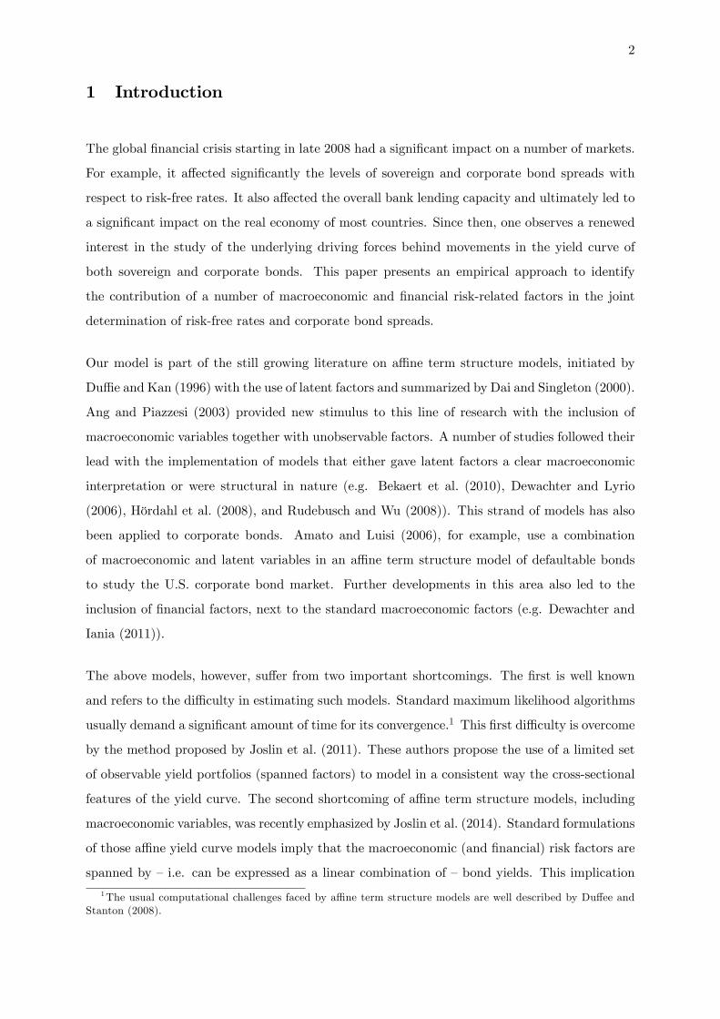
A Macro-Financial Analysis of the Corporate Bond Market�
Hans Dewachtery Leonardo Ianiaz Wolfgang Lemkex Marco Lyrio{
January 2016
Abstract
We assess the contribution of economic and �nancial factors in the determination of euroarea corporate bond spreads over the period 2005-2015. The proposed multi-market, no-arbitrage a¢ ne term structure model is based on the methodology proposed by Dewachter,Iania, Lyrio, and Perea (2015), wich in turn combines the methods introduced by Joslin,Singleton, and Zhu (2011) as well as Joslin, Priebsch, and Singleton (2014). We modeljointly the �risk-free curve�, measured by overnight index swap (OIS) rates, and the corporateyield curves for two rating classes (A and BBB). The model includes four spanned and sixunspanned factors. Based on forecast error variance and historical decompositions we �ndthat, in general, both economic (real activity and in�ation) and �nancial factors (proxyingrisk aversion, �ight to liquidity and general �nancial market stress) play a signi�cant rolein the determination of the risk-free yield curve and corporate bond spreads. For A- andBBB-rated corporate debt, the selected �nancial variables explain on average about 36 and34 percent of their spread variation during the last decade.
JEL classi�cations: E43; E44
Keywords: Euro area corporate bonds; yield spread decomposition; unspanned macro factors.
�The views expressed are those of the authors and do not necessarily re�ect those of the European CentralBank or the National Bank of Belgium. All remaining errors are our own.
yNational Bank of Belgium; Center for Economic Studies, University of Leuven; and CESifo. Address:National Bank of Belgium, de Berlaimontlaan 3, 1000 Brussels, Belgium. Tel.: +32 (0) 2 2215619. Email:[email protected].
zLouvain School of Management. Address: Place de Doyens 1, bte L2.01.02 à 1348 Louvain-la-Neuve, Belgium.Tel.: +32 (0) 10 478439. Email: [email protected].
xEuropean Central Bank. Address: Sonnemannstrasse 20, 60314 Frankfurt am Main, Germany. Tel.: + 49 6913445823. Email: [email protected].
{Insper Institute of Education and Research. Address: Rua Quatá 300, São Paulo, SP - Brazil, 04546-042.Tel.: +55(0)11 45042429. Email: [email protected]. Marco Lyrio is grateful for �nancial support fromthe CNPq-Brazil (Project No. 306373/2013-0).
1
2
1 Introduction
The global �nancial crisis starting in late 2008 had a signi�cant impact on a number of markets.
For example, it a¤ected signi�cantly the levels of sovereign and corporate bond spreads with
respect to risk-free rates. It also a¤ected the overall bank lending capacity and ultimately led to
a signi�cant impact on the real economy of most countries. Since then, one observes a renewed
interest in the study of the underlying driving forces behind movements in the yield curve of
both sovereign and corporate bonds. This paper presents an empirical approach to identify
the contribution of a number of macroeconomic and �nancial risk-related factors in the joint
determination of risk-free rates and corporate bond spreads.
Our model is part of the still growing literature on a¢ ne term structure models, initiated by
Du¢ e and Kan (1996) with the use of latent factors and summarized by Dai and Singleton (2000).
Ang and Piazzesi (2003) provided new stimulus to this line of research with the inclusion of
macroeconomic variables together with unobservable factors. A number of studies followed their
lead with the implementation of models that either gave latent factors a clear macroeconomic
interpretation or were structural in nature (e.g. Bekaert et al. (2010), Dewachter and Lyrio
(2006), Hördahl et al. (2008), and Rudebusch and Wu (2008)). This strand of models has also
been applied to corporate bonds. Amato and Luisi (2006), for example, use a combination
of macroeconomic and latent variables in an a¢ ne term structure model of defaultable bonds
to study the U.S. corporate bond market. Further developments in this area also led to the
inclusion of �nancial factors, next to the standard macroeconomic factors (e.g. Dewachter and
Iania (2011)).
The above models, however, su¤er from two important shortcomings. The �rst is well known
and refers to the di¢ culty in estimating such models. Standard maximum likelihood algorithms
usually demand a signi�cant amount of time for its convergence.1 This �rst di¢ culty is overcome
by the method proposed by Joslin et al. (2011). These authors propose the use of a limited set
of observable yield portfolios (spanned factors) to model in a consistent way the cross-sectional
features of the yield curve. The second shortcoming of a¢ ne term structure models, including
macroeconomic variables, was recently emphasized by Joslin et al. (2014). Standard formulations
of those a¢ ne yield curve models imply that the macroeconomic (and �nancial) risk factors are
spanned by �i.e. can be expressed as a linear combination of �bond yields. This implication
1The usual computational challenges faced by a¢ ne term structure models are well described by Du¤ee andStanton (2008).

3
of standard models is however overwhelmingly rejected by standard regression analysis, which
shows that there is no perfect linear relation between yields and such variables. These authors,
therefore, propose the introduction of macroeconomic variables as unspanned factors in otherwise
standard a¢ ne models. While unspanned factors do not impact directly on bond yields, they
may still have predictive content for risk premiums over and above the information contained in
bond yields. In other words, these factors do not a¤ect the shape of the yield curve but carry
relevant information to forecast excess bond returns.
Our methodology combines the methods proposed by Joslin et al. (2011) and Joslin et al. (2014)
and can be seen as a reduced-form approach of the models proposed by Du¢ e and Singleton
(1999). Such combination has been used previously by Dewachter et al. (2015) in the context
of euro area sovereign bonds. These authors propose a two-market model composed by the OIS
rate, seen as their benchmark market, and the sovereign bond market for a speci�c country of the
euro zone. In this paper we further extend the latter model by modelling several markets at once.
Our focus is on the corporate bond market. The �rst market is representing the benchmark risk-
free rates, measured as the OIS yield curve. The second market is represented by the yield curve
for corporate bonds with A rating, while the third market represents the yield curve of lower-
ranked BBB corporate debt. Due to the availability of data, we only use these two rating classes.
The modeling approach, however, allows the inclusion of as many rating classes as necessary.
The proposed framework is applied to the euro area corporate bond market using monthly data
for the period from July 2005 to April 2015. The relatively short time span is mainly owing
to data availability as the information for some of the maturities of the OIS yield curve is only
available as of July 2005. Our model includes a total of ten factors, six unspanned factors
and four observable factors explaining the OIS rates and the yield curves of corporate bonds of
the two rating classes (A and BBB). The unspanned factors include standard macroeconomic
variables (economic activity and in�ation) and risk-related �nancial factors, which capture the
cost of borrowing for non-�nancial corporations, global tensions, systemic risk, and liquidity
concerns in the �nancial market. To simplify interpretation, these factors are divided in three
groups: economic, �nancial, and idiosyncratic factors.
Our results show that, overall, both economic and risk-related �nancial factors play a signi�-
cant role in the determination of the OIS rate and corporate bond spreads. For the OIS rate,
economic shocks are the most important source of variation for a one-month forecasting hori-
zon and for bonds with maturities up to two years. For intermediate and lower frequencies,
we observe a comparable impact of economic and risk-related �nancial shocks on the OIS rate

4
dynamics. For corporate bond spreads, risk-related �nancial shocks are the dominant drivers
for all frequencies and maturities. The historical decomposition of the OIS yield curve and the
corporate bond spreads show the important contribution of these two groups of factors during
the global �nancial crisis. It also shows that the decrease in corporate bond spreads observed
in 2014 is mainly attributed to a decrease in the contribution of risk-related �nancial factors.
In short, our results emphasize the importance of including also risk-related �nancial factors in
the analysis of corporate bond yields.
The remainder of this paper is organized as follows. Section 2 presents the multi-market, a¢ ne
term structure model and the VAR system used to determine the in�uence of macroeconomic
and risk-related �nancial factors on corporate bond spreads. Section 3 summarizes the data,
describes brie�y the estimation method, and discusses the results. This includes the analysis of
impulse response functions (IRFs), variance decompositions and the historical decomposition of
the OIS rates and corporate bond spreads. Section 4 concludes the paper.
2 The Modelling Framework
Dewachter et al. (2015) combine the methods proposed by Joslin et al. (2011) and Joslin et al.
(2014) and extend the standard a¢ ne yield curve model to a multi-market, single-pricing kernel
framework. In their set-up, one of the markets represents the risk-free yield curve and the
other the sovereign bond market of a speci�c country. This framework is applied to analyse
the developments of sovereign yields in a number of euro area countries (i.e. Belgium, France,
Germany, Italy and Spain) during the sovereign debt crisis period.
In our set-up, the �rst market also represents the risk-free benchmark (the OIS rate). Nev-
ertheless, since our focus is on the corporate bond market, our second and third markets are
represented by the yield curves on corporate bond indices of di¤erent rating classes (A and
BBB).
The framework adopted by Dewachter et al. (2015) is particularly useful since it allows us to
�t the three yield curves with a reasonable precision and also to choose the relevant set of
unspanned factors in order to forecast excess bond returns. Since the methodology is explained
in detail in Dewachter et al. (2015), we restrict ourselves to the modi�cations made in the original
framework to �t our purpose.

5
As is usual in this literature, this type of model imposes the no-arbitrage restriction in the context
of Gaussian and linear state space dynamics under the risk-neutral measure. As suggested by
Joslin et al. (2011), we adopt a limited set of spanned factors � yield portfolios � to model
the cross-sectional of the yield curve. And as suggested by Joslin et al. (2014), we model
the dynamics of the yield portfolios under the historical measure by means of a standard VAR,
including next to the yield curve portfolios a number of macroeconomic and risk-related variables.
Based on the VAR dynamics, and the a¢ ne yield curve representation implied by the risk-neutral
dynamics, we assess the relative contribution of the respective macroeconomic and risk-related
variables in the yield curve dynamics. Below, we describe brie�y the multi-market a¢ ne yield
curve model proposed by Dewachter et al. (2015) and present the assumptions imposed in the
VAR system.
2.1 A multi-market a¢ ne yield curve model for corporate bonds
Joslin et al. (2011) introduce a¢ ne yield curve models using observable yield portfolios as factors
spanning the yield curve. This section is based on Dewachter et al. (2015), who propose a multi-
market version of their model.
It is assumed the existence ofK fundamental and unobserved pricing factors for the yield curve of
all markets (Xk;t) collected in the vector Xt = [X1;t; :::; XK;t]0. These factors re�ect fundamental
sources of risk and their dynamics under the risk-neutral measure (Q) is given by a VAR(1):
Xt = CQX +�
QXXt�1 +�X"
Qt ; "Qt � N(0; IK); (1)
where �QX is a diagonal matrix containing the (assumed) distinct eigenvalues of �QX and �X is a
lower-triangular matrix. We assume that the K factors determine the risk-free interest rate (r0;t)
and each of the market-speci�c, short-term interest rates in market m (rm;t), with m = 1; :::;M ,
as follows:
rm;t = �00 + �
10Xt| {z }
risk-free rate
+mXj=1
sj;t| {z }spreads
(2)
where the �rst two terms, �00+ �10Xt, represent the risk-free rate and sj;t = �
0j + �
1jXt represents
the spreads between bond yields of each rating class and the next rating class with a higher
rating. In this way, the model allows the introduction of several bond markets, all conditioned
on the same risk-neutral probability measure. The di¤erences across bond markets depend on a
constant (�0j ) and the market-speci�c factor sensitivities to the respective fundamental factors,
6
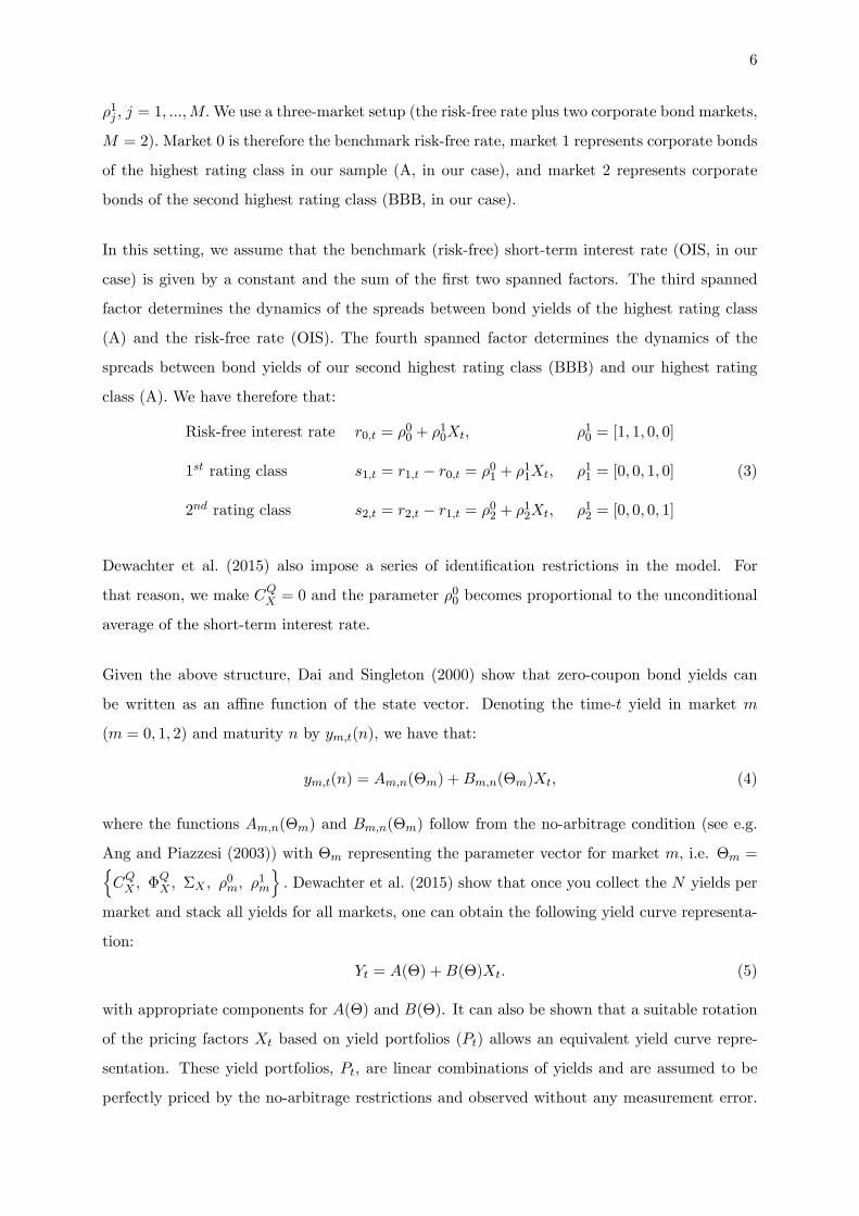
�1j , j = 1; :::;M:We use a three-market setup (the risk-free rate plus two corporate bond markets,
M = 2):Market 0 is therefore the benchmark risk-free rate, market 1 represents corporate bonds
of the highest rating class in our sample (A, in our case), and market 2 represents corporate
bonds of the second highest rating class (BBB, in our case).
In this setting, we assume that the benchmark (risk-free) short-term interest rate (OIS, in our
case) is given by a constant and the sum of the �rst two spanned factors. The third spanned
factor determines the dynamics of the spreads between bond yields of the highest rating class
(A) and the risk-free rate (OIS). The fourth spanned factor determines the dynamics of the
spreads between bond yields of our second highest rating class (BBB) and our highest rating
class (A). We have therefore that:
Risk-free interest rate r0;t = �00 + �
10Xt; �10 = [1; 1; 0; 0]
1st rating class s1;t = r1;t � r0;t = �01 + �11Xt; �11 = [0; 0; 1; 0]
2nd rating class s2;t = r2;t � r1;t = �02 + �12Xt; �12 = [0; 0; 0; 1]
(3)
Dewachter et al. (2015) also impose a series of identi�cation restrictions in the model. For
that reason, we make CQX = 0 and the parameter �00 becomes proportional to the unconditional
average of the short-term interest rate.
Given the above structure, Dai and Singleton (2000) show that zero-coupon bond yields can
be written as an a¢ ne function of the state vector. Denoting the time-t yield in market m
(m = 0; 1; 2) and maturity n by ym;t(n); we have that:
ym;t(n) = Am;n(�m) +Bm;n(�m)Xt; (4)
where the functions Am;n(�m) and Bm;n(�m) follow from the no-arbitrage condition (see e.g.
Ang and Piazzesi (2003)) with �m representing the parameter vector for market m, i.e. �m =nCQX ; �
QX ; �X ; �
0m; �
1m
o: Dewachter et al. (2015) show that once you collect the N yields per
market and stack all yields for all markets, one can obtain the following yield curve representa-
tion:
Yt = A(�) +B(�)Xt: (5)
with appropriate components for A(�) and B(�). It can also be shown that a suitable rotation
of the pricing factors Xt based on yield portfolios (Pt) allows an equivalent yield curve repre-
sentation. These yield portfolios, Pt, are linear combinations of yields and are assumed to be
perfectly priced by the no-arbitrage restrictions and observed without any measurement error.

7
Assuming the yield portfolios are constructed based on a certain matrix W , Pt =WYt, one can
express the yield curve as:
Yt =�I �B(�)(WB(�))�1W
�A(�) +B(�)(WB(�))�1Pt. (6)
2.2 Decomposing the yield curve dynamics
We keep the framework in Dewachter et al. (2015) and adopt a �rst order Gaussian VAR model
to assess the relative importance of macroeconomic and risk-related �nancial shocks in the yield
curve dynamics. Denoting the set of unspanned factors byMt; our VAR(1) model can be written
as: �Mt
Pt
�= CP +�P
�Mt�1Pt�1
�+�
�"PM;t"PP;t
�(7)
where � is a lower-triangular matrix implied by the Cholesky identi�cation of structural shocks.
Below, we describe the variables included in the unspanned and spanned factors.
2.3 Estimation method
Our estimation procedure follows the methodology proposed by Joslin et al. (2011), which is also
described in detail by Dewachter et al. (2015). This methodology uses an e¢ cient factorization
of the likelihood function, arising from the use of yield portfolios as pricing factors. It also
allows for an e¢ cient two-step maximum likelihood estimation procedure, which involves: (i)
the estimation of the VAR system in eq. (7) using standard OLS regressions; and (ii) the
estimation of the the remaining parameters to �t the OIS curve and the bond spread curves for
each rating class using a maximum likelihood procedure.
3 Empirical Results
3.1 Data
We estimate the model on monthly data over the period from July 2005 to April 2015 (118
observations per series). The data used can be sorted in two groups: macro and �nancial
risk-related data and yield curve data.
Macro and �nancial risk-related data. These data are used to construct the six unspanned

8
factors included in the model. They are: (i) the Purchasing Managers� Index (PMI ), which
is based on surveys of business conditions in manufacturing and in services industries. This
index is used directly as our proxy for economic activity in the euro area and is obtained from
Markit Financial Information Services (markit.com); (ii) the year-on-year growth rate of the
Euro area Harmonized Consumer Price Index (INFL) is our measure for in�ation in the euro
area. We collect the data from Datastream; (iii) the spread between the cost of borrowing for
corporations and the average of OIS rates. This is our cost of borrowing factor (COST ) and
the data are from the ECB; (iv) a market volatility index based on EURO STOXX 50 realtime
options prices (VSTOXX ). This is our measure for the general tension in �nancial markets.
The data are collected from STOXX Ltd. (stoxx.com); (v) the Composite Indicator of Systemic
Stress (CISS ) in the �nancial system. This index incorporates a total of 15 �nancial stress
measures and was proposed by Holló et al. (2012). The data are from the European Central
Bank (ECB); and (vi) the spread between the yield on the German government-guaranteed
bond (�Kreditanstalt fur Wiederaufbau�, KfW, a government-owned development bank ) and
the German sovereign bond, averaged across maturities of 1, 2, 3, 4, 5, 7, and 10 years. This
represents our liquidity or �ight-to-liquidity factor (F2L). The data for both series are from
Bloomberg.
Yield curve data. We use the Overnight Index Swap (OIS) rate for maturities of 1, 2, 3, 4, 5,
7, and 10 years, representing the risk-free benchmark rate for the euro area. Finally, we collect
data for two indices of corporate bond yields for the rating classes A and BBB. These indices
are computed by and collected from Bloomberg. We use the same maturities as for the OIS
rate.
3.2 Unspanned and spanned factors
We now formally specify the vectors of unspanned (Mt) and spanned (Pt) factors. The �rst
are used to evaluate the macroeconomic and �nancial forces behind corporate yield spread
movements. The latter are yield portfolios used to explain the dynamics of our benchmark
yield curve (OIS) and the yield curves of the two corporate bond indices representing the rating
classes A and BBB.
Unspanned factors. As mentioned before, we include a total of six unspanned factors. The
�rst two factors re�ect standard macroeconomic conditions of the region and include an indicator
of economic activity (PMI ) and a measure of in�ation (INFL). The last four factors are generally

9
risk-related �nancial factors expressing the cost of borrowing faced by non-�nancial corporations
(COST ), the global tension in �nancial markets (VSTOXX ), the presence of a systemic risk
(CISS ), and the existence of liquidity concerns (F2L). We therefore have the following vector of
unspanned factors:
Mt = [PMIt; INFLt; COSTt ; V STOXXt; CISSt; F2Lt]0 : (8)
Spanned factors. We adopt a total of four spanned factors, i.e. yield portfolios. The �rst
two factors are used to explain the dynamics of the OIS yield curve. They are computed as the
�rst two principal components of the OIS rates for the seven maturities included in the sample
(PCrf;1t and PCrf;2t ). Although we could choose any linear combination of observed yields to
form such portfolios, this choice avoids �tting perfectly a set of speci�c yields and under�tting
the others. The last two factors are used to explain the dynamics of corporate bond spreads.
The �rst of these factors, PCspr;1t , is computed as the �rst principal component of the seven yield
spreads between A bond yields and the OIS rate, one for each maturity. In the same way, the
second of these factors, PCspr;2t , is computed as the �rst principal component of the seven yield
spreads between BBB and A bond yields. The vector of yield portfolios can then be expressed
as:
Pt =hPCrf;1t ; PCrf;2t ; PCspr;1t ; PCspr;2t
i0: (9)
All 10 unspanned and spanned factors can be seen in Figure 1, where the unspanned factors are
standardized. The yield curves for the OIS rate and for the two corporate bond rating classes
are shown in the next section where we evaluate the yield curve �t for each case.
Insert Figure 1: Unspanned and spanned standardized factors
3.3 Model evaluation
The model �ts the OIS and most of maturities of the two corporate bond yield curves rather
well.2 This can be seen in Figures 2-7. Figure 2 shows the �t of the OIS yield curve. Since
the observed data (continuous line) is almost indistinguishable from the �tted values (dashed
line), we display the �tting errors separately in Figure 3. We do the same for the A and BBB
bond spread curves in Figures 4-7. Summary statistics of these �tting errors are provided in the
last three columns of Table 1. Overall, we �nd that these �tting errors are quite low, as usually
found in the literature for a¢ ne term structure models (see e.g. Ang and Piazzesi (2003)). The
2The parameter estimates of the model are available upon request.

10
standard deviation of the �tting errors are mostly below 10 bp, reaching a maximum of 29 bp
for the 10-yr A bond yield spread. Such �t for all yield curves is achieved with a relatively small
number of spanned factors. Nevertheless, the �rst-order autocorrelation of the �tting errors
(last column of Table 1) are rather high in all cases, potentially indicating the need for an extra
factor.
Insert Figures 2-7: Yield curve �t and �tting errors
Insert Table 1: Summary statistics of OIS rates and corporate bond spreads
We also compare the risk premiums for the OIS, A and BBB yield curves for a one-year holding
period with the realized excess return for the same holding period 3 (Figures 8 to 10). The
computation of the risk premium is shown in Appendix A. In all cases, we see a reasonably
good �t, deteriorating somehow for long-term maturities. Table 2 shows the summary statistics
for those risk premiums and realized excess returns. We observe that for all maturities the
realized excess return is more volatile than the risk premium. Our model performs rather
well in replicating observed excess returns. For all maturities the correlation between the risk
premium and the realized excess return is above 0.72 reaching a value of 0.96 for a two-year
BBB bond.
Insert Figures 8-10: Fit of the risk premium
Insert Table 2: Summary statistics of risk premiums and realized excess returns
Finally, it is interesting to observe the risk premium di¤erential between corporate bonds and
our benchmark risk-free rate. This is shown in Figures 11 and 12 for A- and BBB-rated corporate
bonds, respectively. These �gures show that for both rating classes the risk premium di¤erential
increases with maturity. As expected, we also observe a sharp increase in the risk premium
di¤erential after the beginning of the 2008 �nancial crisis.
Insert Figures 11-12: Risk premium di¤erential
Next, we focus on the dynamics of corporate bond yield spreads as a function of our ten un-
spanned and spanned factors. This is done through the analysis of IRFs, variance decompositions
and historical decompositions. In order to facilitate interpretation, for the last two exercises, we
divide the ten factors in three groups, as explained below.
3For every rating class, the risk premium is obtained under the condition of no default, i.e. it is assumed thatthe rating class considered does not default over considered the holding period.

11
3.4 Impulse response functions
The model includes a large number of parameters. Therefore, instead of discussing the parameter
estimates we analyse the dynamic properties of the model by means of IRFs. This allows us to
visualize the response of corporate bond yield spreads to a one standard deviation shock to each
of the 10 variables included in the model. The ordering of such variables in the VAR system
de�ned above (eq. (7)) is as follows:
Ft = [PMIt; INFLt; COSTt ; V STOXXt; CISSt; F2Lt;
PCrf;1t ; PCrf;2t ; PCspr;1t ; PCspr;2t
i0: (10)
We start with the unspanned factors followed by the spanned factors. The unspanned factors
include �rst the variables representing the macroeconomic situation of the euro area and then
the risk-related �nancial factors. The estimated VAR(1) system under the historical (P) measure
is as follows:
Ft = CPF +�
PFFt�1 +�F "
PF;t; (11)
where �F is a lower-triangular matrix implied by the lower triangular identi�cation of the shocks.
Figures 13 and 14 show the IRFs for the 5-year corporate bond yield spreads for the A and BBB
rating classes, respectively. These �gures also show the 90% con�dence interval (dashed lines)
obtained by a standard bootstrapping procedure. The horizontal axis is expressed in months.
Despite the high dimension of the VAR system, most of the IRFs are in line with economic
intuition. First, we analyse the impact of shocks to the macroeconomic condition in the euro
area. We see that in both cases (A and BBB bonds) a one-standard deviation shock to the PMI
index, representing an improvement in the economic activity, initially decreases corporate bond
spreads in a signi�cant way. The quantitative impact is, however, rather small and signi�cant
only up to around six months after the shock. The impact of this shock reaches a maximum
of 10 basis points in the case of BBB bonds. In the case of an in�ation shock (INFL), the
initial reaction is negative and counterintuive. Nevertheless, its magnitude is very small and not
signi�cant.
We now analyse the e¤ect of shocks to the risk-related �nancial factors. In both cases, a one-
standard deviation shock to the cost of borrowing (COST ) has an initial signi�cant and positive
impact on bond spreads. That is expected but its magnitude seems rather small (around �ve
basis points for BBB bonds). Shocks to the VSTOXX index have the greatest impact on bond

12
spreads. A shock to this index, and therefore an increase in the uncertainty in �nancial markets,
initially increases corporate bond spreads. For BBB bonds, this shock has an initial impact of
15 basis points. This impact is signi�cant for the �rst six months after the shock for both bond
classes. Although the initial e¤ect of a shock to our systemic risk measure (CISS ) is marginally
negative, and therefore counterintuitive, it is not signi�cant. Its e¤ect on bond spreads only
becomes positive and marginally signi�cant after approximately one year. Finally, shocks to our
proxy for liquidity concerns in the �nancial market (F2L) do not seem to have an immediate
impact on bond spreads. After around 10 months, however, its impact is signi�cant and positive
(as expected) reaching close to 10 basis points for BBB bonds.
Insert Figures 13-14: Impulse response functions
3.5 Variance decompositions
One constructs variance decompositions in order to assess the relative contribution of each
factor to forecast variances. Since we have a total of 10 factors in the model, in order to fa-
cilitate interpretation, we divide these factors in three groups: (i) economic factors summarize
the overall economic condition of the euro area and the dynamics of the risk-free rate (PMI,
INFL; PCrf;1t ; PCrf;2t ); (ii) risk-related �nancial factors capture global tensions, systemic risk,
and liquidity concerns in the �nancial market and the cost of borrowing for non-�nancial cor-
porations (COST; V STOXX; CISS; F2L); and (iii) idiosyncratic factors include the residual
dynamics not explained by economic or risk-related �nancial factors (PCspr;1 and PCspr;2).
Figure 15 shows the variance decomposition of the OIS yield curve. Economic shocks are the
most important source of variation for short-term maturities (up to two years) and for very short
forecasting horizons (one month). For longer maturities, but still short forecasting horizons, risk-
related �nancial factors become the dominant driver behind the OIS rate dynamics. For longer
forecasting horizons, both groups of shocks (economic and risk-related) have roughly the same
impact on the OIS rate.
Regarding corporate bond spreads, Figures 16 and 17 show for all maturities the variance de-
compositions of A and BBB bond spreads, respectively. First, we note that both economic and
risk-related �nancial shocks are signi�cant sources of variation in corporate bond yield spreads.
Nevertheless, in both cases (A and BBB bonds), we note that movements in corporate bond
spreads are mostly attributed to risk-related �nancial shocks. For all maturities and long fore-

13
casting horizons (ten years), risk-related shocks are responsible for approximately 50% of the
forecast variance of corporate bond spreads. These results emphasize the importance of includ-
ing such factors in the analysis of corporate bond yields. Economic factors, on the other hand,
have a slightly increasing role in the forecast variance as the forecast horizon increases. Such
factors are responsible for approximately 30% of the variation in bond spreads at long forecasting
horizons.
Insert Figure 15-17: Variance decompositions
3.6 Historical decomposition of bond yield spreads
The variance decompositions discussed above show the importance of both economic and risk-
related �nancial factors in the forecast variances of corporate bond spreads. We would like,
however, to visualize the contribution over time of each group of factors to the OIS rate and
corporate bond spreads. Figures 17 to 19 show the historical decomposition over our sample
period of the 5-year OIS rate and the 5-year A and BBB corporate bond spreads, respectively.
Each panel shows the contribution of a speci�c group of shocks (economic, risk-related, and
idiosyncratic) to the total yield or yield spread.
First, we analyse the evolution of the 5-yr OIS rate, our benchmark risk-free rate (Figure 18).
The importance of both economic and risk-related �nancial factors in the determination of such
rate is striking. We also observe that the recent decrease in the risk-free rate (after 2014), can be
mainly attributed to the economic situation in the euro area. When we analyse the components
of the economic group of shocks separately, we observe that this decrease is mainly attributed to
in�ation.4 During the same period, risk-related �nancial factors had a somehow stable in�uence
on the OIS rate.
Looking at the corporate bond spreads (Figures 19 and 20), we see the importance of risk-related
�nancial shocks, especially around the end of 2008 under the in�uence of the global �nancial
crisis. The in�uence of risk-related �nancial factors can also be observed during the decrease
in corporate bond spreads which took place from the third quarter of 2012 until the beginning
of 2015. Note that throughout 2014 the impact of such factors on bond spreads was mainly
negative. One could conjecture that the calming down of the markets since the end of 2012 was
inter alia driven by the Outright Monetary Transactions (OMT) programme announced by the
ECB in September 2012. Nevertheless, in April 2015 (the end of our sample period) such factors
4The historical decomposition of all series presented per factor (10 in total) is available upon request.

14
are again responsible for a substantial part of corporate bond spreads. In summary, although
economic factors have a signi�cant impact on bond spreads during most of our sample period,
our results show that, in general, risk-related �nancial factors play a very important role in the
dynamics of corporate bond spreads.
Insert Figures 18-20: Historical decompositions
4 Conclusion
This paper introduces a modeling framework for capturing the joint arbitrage-free dynamics
of the risk-free term structure and corporate bond yield curves of various rating classes. The
approach is based on methods proposed by Joslin et al. (2011), Joslin et al. (2014), and Dewachter
et al. (2015).
We apply this multi-market term structure model for analyzing the development of A- and BBB-
rated euro area corporate bond spreads over the last decade, thereby focusing on the global
�nancial crisis. The empirical model features overall ten factors, of which four are �spanned�,
explaining the cross section (maturity structure) of risk-free and corporate yields, while the
remaining six �unspanned�factors help to explain the dynamics of the spanned factors and can
hence account for time variation in bond risk premiums. Our spanned factors are essentially
portfolios of risk-free and corporate bond yields, while the unspanned factors represent macro-
economic driving forces (real activity and in�ation) as well as �nancial factors, which capture risk
aversion, investors�liquidity preferences and bouts of general stress levels in �nancial markets.
We �nd that both macroeconomic and �nancial factors are important driving forces for the
risk-free yield curve and corporate bond spreads. According to the historical decomposition,
both macroeconomic and �nancial factors are responsible on average for 42 percent each of the
variation across the OIS yield curve, over our entire sample. Idiosyncratic shocks explain the
remaining 16 percent of this variation. For corporate bond spreads, macroeconomic factors
explain about 44 and 46 percent of the unexpected �uctuations in A- and BBB-rated corporate
bond spreads, respectively, over the sample and across all maturities. Our �nancial factors are
responsible for 36 and 34 percent of the respective variation while both for A and BBB bonds
the remaining 20 percent are explained by idiosyncratic factors.
The paper carries the idea of modeling bond yields via spanned and unspanned factors further

15
to corporate bonds. The evidence that we �nd for the relevance of unspanned observable factors
mirrors similar �ndings in the literature that focuses solely on government bonds. A natural
extension of the presented framework is to also include government debt markets in order to
shed light on the sovereign-corporate nexus, i.e. how strongly sovereign debt market tensions
feed back towards the corporate sector and vice versa.
References
Amato, J. D. and M. Luisi (2006). Macro factors in the term structure of credit spreads. BIS
Working Papers 203, Bank for International Settlements.
Ang, A. and M. Piazzesi (2003). A no-arbitrage vector autoregression of term structure dynamics
with macroeconomic and latent variables. Journal of Monetary Economics 50 (4), 745�787.
Bekaert, G., S. Cho, and A. Moreno (2010). New-Keynesian macroeconomics and the term
structure. Journal of Money, Credit and Banking 42, 33�62.
Dai, Q. and K. J. Singleton (2000). Speci�cation analysis of a¢ ne term structure models. The
Journal of Finance 55 (5), 1943�1978.
Dewachter, H. and L. Iania (2011). An extended macro-�nance model with �nancial factors.
Journal of Financial and Quantitative Analysis 46, 1893�1916.
Dewachter, H., L. Iania, M. Lyrio, and M. d. S. Perea (2015). A macro-�nancial analysis of the
euro area sovereign bond market. Journal of Banking and Finance 50, 308�325.
Dewachter, H. and M. Lyrio (2006). Macro factors and the term structure of interest rates.
Journal of Money, Credit and Banking 38 (1), 119�140.
Du¤ee, G. R. and R. H. Stanton (2008). Evidence on simulation inference for near unit-root
processes with implications for term structure estimation. Journal of Financial Economet-
rics 6 (1), 108�142.
Du¢ e, D. and R. Kan (1996). A yield-factor model of interest rates. Mathematical Finance 6,
379½U406.
Du¢ e, D. and K. J. Singleton (1999). Modeling term structures of defaultable bonds. Review
of Financial Studies 12 (4), 687�720.
Holló, D., M. Kremer, and M. L. Duca (2012). CISS - a composite indicator of systemic stress
in the �nancial system. ECB working paper series, European Central Bank.

16
Hördahl, P., O. Tristani, and D. Vestin (2008). The yield curve and macroeconomic dynamics.
Economic Journal 118 (533), 1937�1970.
Joslin, S., M. Priebsch, and K. J. Singleton (2014). Risk premiums in dynamic term structure
models with unspanned macro risks. Journal of Finance 69 (3), 1197�1233.
Joslin, S., K. J. Singleton, and H. Zhu (2011). A new perspective on Gaussian dynamic term
structure models. Review of Financial Studies 24 (3), 926�970.
Rudebusch, G. D. and T. Wu (2008). A macro-�nance model of the term structure, monetary
policy and the economy. The Economic Journal 118, 906�926.

17
Appendix A - Risk premium computation
This appendix shows the computations for the risk premium (rp) considering a one-year (12
months) holding period.
1. Bonk risk premium
ym;t = Am +BmXt
Xt = �+�Xt +�"t
pm;t = �ym;tm
= �Amm
� BmmXt
E(pm�12;t+12) = �ym;tm
= � Am�12m� 12 �
Bm�12m� 12E(Xt+12)
rpt+12;t = E(pm�12;t+12)� pm;t � y12;t
where
E(Xt+12) = �+�Xt+11 = �+��+�2Xt+10 =
= �
11Xj=0
�j +�12Xt
rpt+12;t = E(pm�12;t+12)� pm;t � y12;t
= � Am�12m� 12 �
Bm�12m� 12E(Xt+12) +
Amm
+BmmXt �
A1212
� B1212Xt
= � Am�12m� 12 �
Bm�12m� 12[�
11Xj=0
�j +�12Xt] +Amm
+BmmXt �
A1212
� B1212Xt
= � Am�12m� 12 �
Bm�12m� 12�
11Xj=0
�j +Amm
� A1212
� Bm�12m� 12�
12Xt +BmmXt �
B1212Xt
= � Am�12m� 12 �
Bm�12m� 12�
11Xj=0
�j +Amm
� A1212
+ [�Bm�12m� 12�
12 +Bmm
� B1212]Xt
2. Risk premium per rating
rpOISt+12;t = �AOISm�12m� 12 �
BOISm�12m� 12�
11Xj=0
�j +AOISm
m� A
OIS12
12+ [�
BOISm�12m� 12�
12 +BOISm
m� B
OIS12
12]Xt
rpjt+12;t = �Ajm�12m� 12 �
Bjm�12m� 12�
11Xj=0
�j +Ajmm
� Aj12
12+ [�
Bjm�12m� 12�
12 +Bjmm
� Bj12
12]Xt
j = A; BBB

18
3. Risk premium di¤erential
The risk premium di¤erential is computed as the di¤erence betwwen the risk premium on a
speci�c corporate bond (A and BBB) and the risk premium on the benchmark risk-free rate
(OIS rate).
rpj�OIS = rpjt+12;t � rpOISt+12;t where j = A; BBB

19
Table 1: Summary statistics of OIS rates and corporate bond spreads
Mean Std Fitting errordata (%) emp. (%) data (%) emp. (%) mean (bp) std (bp) auto
OISyield1yr 1.55 1.54 1.60 1.61 2 7 0.82yield2yr 1.69 1.70 1.57 1.56 -1 3 0.71yield3yr 1.85 1.86 1.53 1.52 -1 5 0.78yield4yr 2.01 2.01 1.48 1.48 0 4 0.82yield5yr 2.16 2.16 1.43 1.43 1 3 0.81yield7yr 2.44 2.43 1.33 1.35 1 3 0.87yield10yr 2.77 2.78 1.23 1.22 -1 6 0.84
Aspread1yr 0.58 0.81 0.49 0.47 -23 12 0.85spread2yr 0.65 0.81 0.46 0.47 -16 7 0.82spread3yr 0.71 0.81 0.43 0.47 -10 8 0.85spread4yr 0.79 0.81 0.48 0.47 -2 5 0.77spread5yr 0.87 0.81 0.52 0.47 6 8 0.89spread7yr 0.94 0.81 0.48 0.47 13 8 0.82spread10yr 1.09 0.79 0.50 0.47 29 11 0.86
BBBspread1yr 0.85 0.96 0.73 0.97 -10 30 0.95spread2yr 1.06 1.07 0.78 0.96 -2 20 0.95spread3yr 1.26 1.19 0.87 0.96 7 14 0.94spread4yr 1.40 1.30 0.93 0.95 9 10 0.91spread5yr 1.56 1.41 1.00 0.95 15 10 0.83spread7yr 1.71 1.63 1.09 0.94 8 16 0.94spread10yr 1.85 1.92 1.06 1.93 -8 23 0.94
Note: Mean denotes the sample arithmetic average, std the standard deviation, auto the �rst-ordermonthly autocorrelation, and emp the empirical result from the model.

20
Table 2: Summary statistics of risk premiums and realized excess returns
Mean Std rp� rerrp (%) rer (%) rp (%) rer (%) mean (%) std (%) auto corr
OISyield2yr 0.66 0.69 0.82 1.12 -0.04 0.70 0.85 0.78yield3yr 1.32 1.39 1.44 2.03 -0.07 1.30 0.84 0.77yield4yr 1.97 2.06 1.93 2.81 -0.10 1.84 0.84 0.76yield5yr 2.59 2.71 2.35 3.51 -0.12 2.34 0.84 0.75yield7yr 3.70 3.86 3.06 4.79 -0.16 3.28 0.84 0.73yield10yr 5.03 5.23 3.96 6.44 -0.21 4.50 0.84 0.72
Ayield2yr 1.50 1.52 1.38 1.51 -0.02 0.59 0.84 0.92yield3yr 2.15 2.19 2.21 2.48 -0.04 1.12 0.84 0.89yield4yr 2.79 2.84 3.00 3.38 -0.05 1.65 0.84 0.87yield5yr 3.40 3.46 3.75 4.26 -0.06 2.20 0.84 0.86yield7yr 4.48 4.56 5.24 6.00 -0.08 3.30 0.84 0.84yield10yr 5.75 5.83 7.40 8.49 -0.08 4.91 0.85 0.82
BBByield2yr 1.92 1.94 2.32 2.36 -0.01 0.64 0.85 0.96yield3yr 2.82 2.84 3.62 3.70 -0.02 1.30 0.85 0.94yield4yr 3.69 3.72 4.91 5.04 -0.03 1.99 0.85 0.92yield5yr 4.52 4.55 6.19 6.38 -0.04 2.71 0.86 0.91yield7yr 6.03 6.06 8.74 9.09 -0.04 4.22 0.86 0.89yield10yr 7.89 7.91 12.46 13.08 -0.02 6.48 0.86 0.87
Note: The table shows the summary statistics for the risk premium (rp) and realized excess return(rer ) for the OIS rate and A- and B-rated corporate bonds considering a one-year holding period. Thesample period goes from July 2005 to April 2015 (monthly, 118 obs.). The statistics, however, do notinclude the last 12 months for which we cannot compute the realized excess return 12 months ahead.Mean denotes the sample arithmetic average, std the standard deviation, auto the �rst-order monthlyautocorrelation, and corr the correlation between the rp and rer series.

Figure 1: Unspanned and spanned standardized factors
Note: The �gure shows the 6 unspanned and 4 spanned factors. The unspanned factors are standardized:PMI is the Purchasing Managers�Index, which is based on surveys of business conditions in manufacturingand in services industries (source: markit.com); INFL is the year-on-year growth rate of the Euro areaConsumer Price Index (source: Datastream); COST is the spread between the cost of borrowing for corpo-rations and the average of OIS rates (source: ECB); VSTOXX is a market volatility index based on EUROSTOXX 50 realtime options prices (source: stoxx.com); CISS is the Composite Indicator of Systemic Stressin the �nancial system which incorporates 15 �nancial stress measures (source: Holló, Kremer, and Lo Duca(2012)); and F2L is the spread between the yield on the German government guaranteed bond (KfW) andthe German sovereign bond, averaged across maturities (source: Bloomberg). The spanned factors are thefollowing: PC(rf,1) and PC(rf,2) are the �rst two principal components of the OIS rates for the seven ma-turities included in the sample (1, 2, 3, 4, 5, 7, 10 years); PC(spr,1) is the �rst principal component of theseven yield spreads between A bond yields and the OIS rate; and PC(spr,2) is the �rst principal componentof the seven yield spreads between BBB and A bond yields. For all series, the sample period goes from July2005 to April 2015 (monthly, 118 obs.).
1
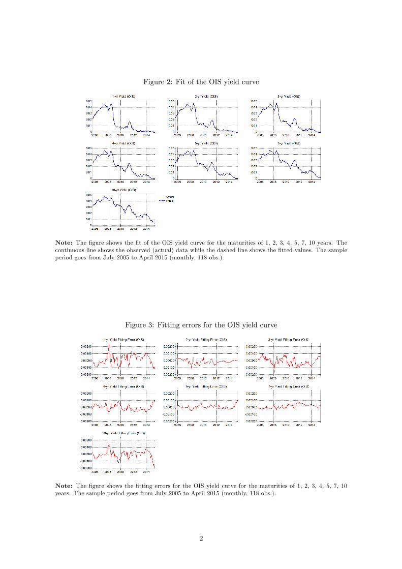
Figure 2: Fit of the OIS yield curve
Note: The �gure shows the �t of the OIS yield curve for the maturities of 1, 2, 3, 4, 5, 7, 10 years. Thecontinuous line shows the observed (actual) data while the dashed line shows the �tted values. The sampleperiod goes from July 2005 to April 2015 (monthly, 118 obs.).
Figure 3: Fitting errors for the OIS yield curve
Note: The �gure shows the �tting errors for the OIS yield curve for the maturities of 1, 2, 3, 4, 5, 7, 10years. The sample period goes from July 2005 to April 2015 (monthly, 118 obs.).
2

Figure 4: Fit of the A bond yield spread
Note: The �gure shows the �t of the spread between the A bond yield and the OIS rate for the maturitiesof 1, 2, 3, 4, 5, 7, 10 years. The continuous line shows the observed (actual) data while the dashed lineshows the �tted values. The sample period goes from July 2005 to April 2015 (monthly, 118 obs.).
Figure 5: Fitting errors for the A bond yield spreads
Note: The �gure shows the �tting errors for the spread between the A bond yield and the OIS rate.for thematurities of 1, 2, 3, 4, 5, 7, 10 years. The sample period goes from July 2005 to April 2015 (monthly, 118obs.).
3
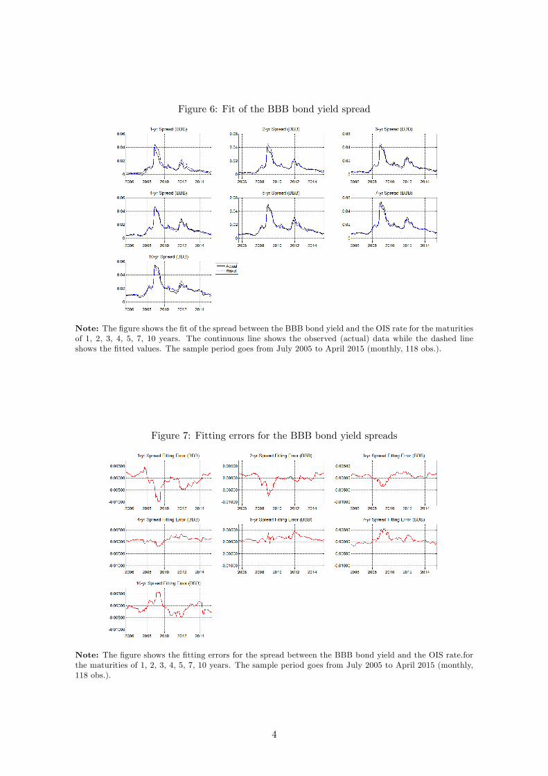
Figure 6: Fit of the BBB bond yield spread
Note: The �gure shows the �t of the spread between the BBB bond yield and the OIS rate for the maturitiesof 1, 2, 3, 4, 5, 7, 10 years. The continuous line shows the observed (actual) data while the dashed lineshows the �tted values. The sample period goes from July 2005 to April 2015 (monthly, 118 obs.).
Figure 7: Fitting errors for the BBB bond yield spreads
Note: The �gure shows the �tting errors for the spread between the BBB bond yield and the OIS rate.forthe maturities of 1, 2, 3, 4, 5, 7, 10 years. The sample period goes from July 2005 to April 2015 (monthly,118 obs.).
4

Figure 8: Fit of the risk premium: OIS yield curve
Note: The �gure considers a one-year holding period. It shows the risk premium (continuous line) and therealized excess return (dashed line) for the OIS rates with maturities of 1, 2, 3, 4, 5, 7, 10 years. The sampleperiod goes from July 2005 to April 2015 (monthly, 118 obs.).
Figure 9: Fit of the risk premium: A bond yield curve
Note: The �gure considers a one-year holding period. It shows the risk premium (continuous line) and therealized excess return (dashed line) for the A bond yields with maturities of 1, 2, 3, 4, 5, 7, 10 years. Thesample period goes from July 2005 to April 2015 (monthly, 118 obs.).
5

Figure 10: Fit of the risk premium: BBB bond yield curve
Note: The �gure considers a one-year holding period. It shows the risk premium (continuous line) and therealized excess return (dashed line) for the BBB bond yields with maturities of 1, 2, 3, 4, 5, 7, 10 years. Thesample period goes from July 2005 to April 2015 (monthly, 118 obs.).
Figure 11: Risk premium di¤erential: A bond yields wrt OIS rate
Note: The �gure considers a one-year holding period. It shows the risk premium di¤erential between Abonds and our benchmark risk-free rate (the OIS rate). This is done for bond yields with maturities of 1, 2,3, 4, 5, 7, 10 years. The sample period goes from July 2005 to April 2015 (monthly, 118 obs.).
6

Figure 12: Risk premium di¤erential: BBB bond yields wrt OIS rate
Note: The �gure considers a one-year holding period. It shows the risk premium di¤erential between BBBbonds and our benchmark risk-free rate (the OIS rate). This is done for bond yields with maturities of 1, 2,3, 4, 5, 7, 10 years. The sample period goes from July 2005 to April 2015 (monthly, 118 obs.).
7

Figure 13: Impulse response function: Response of the 5-yr A bond yield spread to factor shocks
Note: The �gure shows the impulse responses of 5-year A bond yield spreads for the maturities of 1, 2, 3, 4,5, 7, 10 years to a one-standard deviation shock in each of the 10 factos (six unspanned and four spanned).The dashed lines show the 90% con�dence interval. Error bands are obtained by a standard bootstrappingprocedure.
Figure 14: Impulse response function: Response of the 5-yr BBB bond yield spread to factorshocks
Note: The �gure shows the impulse responses of 5-year BBB bond yield spreads for the maturities of 1, 2, 3,4, 5, 7, 10 years to a one-standard deviation shock in each of the 10 factos (six unspanned and four spanned).The dashed lines show the 90% con�dence interval. Error bands are obtained by a standard bootstrappingprocedure.
8
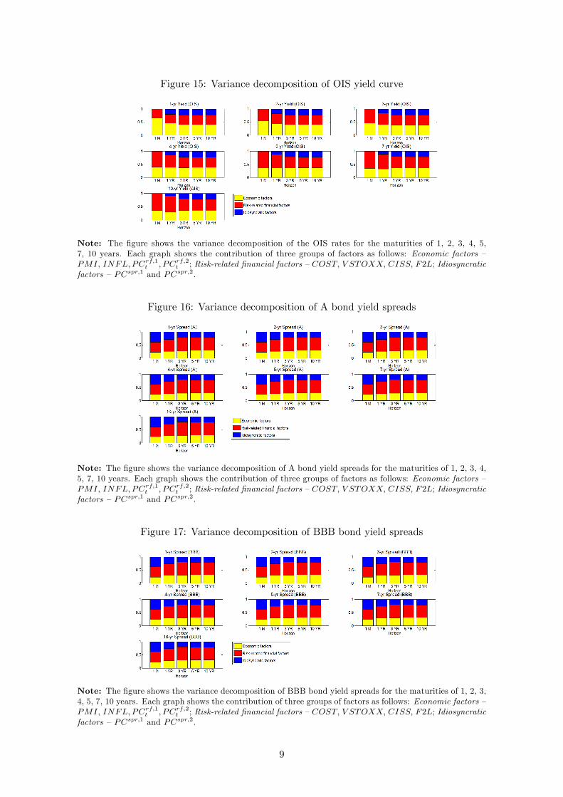
Figure 15: Variance decomposition of OIS yield curve
Note: The �gure shows the variance decomposition of the OIS rates for the maturities of 1, 2, 3, 4, 5,7, 10 years. Each graph shows the contribution of three groups of factors as follows: Economic factors �PMI, INFL;PCrf;1t ; PCrf;2t ; Risk-related �nancial factors �COST; V STOXX; CISS; F2L; Idiosyncraticfactors �PCspr;1 and PCspr;2.
Figure 16: Variance decomposition of A bond yield spreads
Note: The �gure shows the variance decomposition of A bond yield spreads for the maturities of 1, 2, 3, 4,5, 7, 10 years. Each graph shows the contribution of three groups of factors as follows: Economic factors �PMI, INFL;PCrf;1t ; PCrf;2t ; Risk-related �nancial factors �COST; V STOXX; CISS; F2L; Idiosyncraticfactors �PCspr;1 and PCspr;2.
Figure 17: Variance decomposition of BBB bond yield spreads
Note: The �gure shows the variance decomposition of BBB bond yield spreads for the maturities of 1, 2, 3,4, 5, 7, 10 years. Each graph shows the contribution of three groups of factors as follows: Economic factors �PMI, INFL;PCrf;1t ; PCrf;2t ; Risk-related �nancial factors �COST; V STOXX; CISS; F2L; Idiosyncraticfactors �PCspr;1 and PCspr;2.
9

Figure 18: Historical decomposition of 5-yr OIS rate
Note: The �gure shows the historical decomposition of the 5-year OIS rate with the shocks grouped asfollows: Economic shocks �PMI, INFL;PCrf;1t ; PCrf;2t ; Risk-related �nancial shocks �COST; V STOXX;CISS; F2L; and Idiosyncratic shocks �PCspr;1 and PCspr;2.
Figure 19: Historical decomposition of 5-yr A bond yield spread
Note: The �gure shows the historical decomposition of the 5-year A bond yield spread with the shocksgrouped as follows: Economic shocks �PMI, INFL;PCrf;1t ; PCrf;2t ; Risk-related �nancial shocks �COST;V STOXX; CISS; F2L; and Idiosyncratic shocks �PCspr;1 and PCspr;2.
10

Figure 20: Historical decomposition of 5-yr BBB bond yield spread
Note: The �gure shows the historical decomposition of the 5-year BBB bond yield spread with the shocksgrouped as follows: Economic shocks �PMI, INFL;PCrf;1t ; PCrf;2t ; Risk-related �nancial shocks �COST;V STOXX; CISS; F2L; and Idiosyncratic shocks �PCspr;1 and PCspr;2.
11